


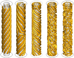



1. Introduction
Thermal convection induced by electric fields in dielectric fluids has attracted significant attention from many researchers over the last few decades due to its promising potential applications in geophysics (Hart, Glatzmaier & Toomre, Reference Hart, Glatzmaier and Toomre1986; Futterer et al. Reference Futterer, Krebs, Plesa, Zaussinger, Hollerbach, Breuer and Egbers2013) and in heat exchange systems (Allen & Karayiannis, Reference Allen and Karayiannis1995; Laohalertdecha, Naphon & Wongwises, Reference Laohalertdecha, Naphon and Wongwises2007). Indeed, when a high-frequency electric voltage is imposed on a dielectric fluid with a temperature gradient, a dielectrophoretic (DEP) force is generated (Landau & Lifshitz, Reference Landau and Lifshitz1984), and it can lead to thermoelectric convective flow (Roberts, Reference Roberts1969; Turnbull, Reference Turnbull1969; Chandra & Smylie, Reference Chandra and Smylie1972; Yoshikawa, Crumeyrolle & Mutabazi, Reference Yoshikawa, Crumeyrolle and Mutabazi2013; Travnikov, Crumeyrolle & Mutabazi, Reference Travnikov, Crumeyrolle and Mutabazi2015, Reference Travnikov, Crumeyrolle and Mutabazi2016; Mutabazi et al. Reference Mutabazi, Yoshikawa, Fogaing, Travnikov, Crumeyrolle, Futterer and Egbers2016). The thermoelectrohydrodynamic (TEHD) convection induced by the DEP force has been demonstrated in experiments conducted in the microgravity environment of Spacelab 3 onboard the space shuttle Challenger (Hart et al. Reference Hart, Glatzmaier and Toomre1986), in the GeoFlow experiments performed under microgravity conditions on the International Space Station (ISS) (Futterer et al. Reference Futterer, Gellert, Von Larcher and Egbers2008, Reference Futterer, Krebs, Plesa, Zaussinger, Hollerbach, Breuer and Egbers2013), in parabolic flight experiments with 22-second periods of microgravity (Dahley et al. Reference Dahley, Futterer, Egbers, Crumeyrolle and Mutabazi2011; Meyer et al. Reference Meyer, Jongmanns, Meier, Egbers and Mutabazi2017, Reference Meyer, Crumeyrolle, Mutabazi, Meier, Jongmanns, Renoult, Seelig and Egbers2018, Reference Meyer, Meier, Jongmanns, Seelig, Egbers and Mutabazi2019; Meier et al. Reference Meier, Jongmanns, Meyer, Seelig, Egbers and Mutabazi2018) and recently in sounding rocket flight with a microgravity phase of six minutes (Meyer et al. Reference Meyer, Meier, Motuz and Egbers2023).
In recent years, particular attention has focused on theoretical investigations of THED convection in a dielectric fluid inside a cylindrical annular cavity under microgravity conditions. Yoshikawa et al. (Reference Yoshikawa, Crumeyrolle and Mutabazi2013) solved the linear stability problem of the thermal convection driven by the DEP force under microgravity conditions and found that the critical modes are stationary and non-axisymmetric (helices). The critical electric Rayleigh number, based on an electric gravity, and the critical wavenumber depend sensitively on the radius ratio. Travnikov et al. (Reference Travnikov, Crumeyrolle and Mutabazi2015, Reference Travnikov, Crumeyrolle and Mutabazi2016) performed three-dimensional (3-D) numerical simulations with periodic boundary conditions. These authors showed that the bifurcation from the base state to convective flow is supercritical and that the Nusselt number characterizing the heat transfer induced by the DEP force is sensitive to the Prandtl number (Pr) and the radius ratio (η). Futterer et al. (Reference Mutabazi, Yoshikawa, Fogaing, Travnikov, Crumeyrolle, Futterer and Egbers2016) experimentally studied heat transfer in a vertical annulus with a finite length subject to the DEP force under Earth's conditions and found that the DEP force enhances heat transfer. Meyer et al. (Reference Meyer, Jongmanns, Meier, Egbers and Mutabazi2017) addressed the stability problem of a dielectric liquid with a high Prandtl number under the combined influence of the Earth's gravity and electric gravity. Their theoretical analysis revealed that the critical mode is stationary columnar vortices with axes parallel to the cylinder axis under the Earth's gravity, whereas it consists of inclined stationary (helical) vortices under microgravity conditions. Experiments performed in parabolic flight (Meyer et al. Reference Meyer, Jongmanns, Meier, Egbers and Mutabazi2017) and more recently in sounding rocket flight (Meyer et al. Reference Meyer, Meier, Motuz and Egbers2023) confirmed the existence of non-axisymmetric modes. Since then, Meyer et al. (Reference Meyer, Crumeyrolle, Mutabazi, Meier, Jongmanns, Renoult, Seelig and Egbers2018) carried out numerical simulations of the problem incorporating time-varying axial gravity, which corresponds to the parabolic flight scenario, with forces ranging from 0 g to ~1.8 g. These simulations revealed that the thermoelectric convection generated during a precedent hypergravity phase is not completely dissipated during the microgravity phase and affects the evaluation of the heat transfer. Meier et al. (Reference Meier, Jongmanns, Meyer, Seelig, Egbers and Mutabazi2018) and Meyer et al. (Reference Meyer, Meier, Motuz and Egbers2023) utilized two different measurement techniques (particle image velocimetry (PIV) and the shadowgraph technique) to determine the structure and temperature distribution of the flow and hence gained a better understanding of the flow patterns and heat transfer. These experimental results exhibited a good qualitative agreement with linear stability theory (Yoshikawa et al. Reference Yoshikawa, Crumeyrolle and Mutabazi2013; Meyer et al. Reference Meyer, Jongmanns, Meier, Egbers and Mutabazi2017) and numerical simulations (Travnikov et al. Reference Travnikov, Crumeyrolle and Mutabazi2015).
Recently, the authors of this work studied thermoelectric convection in a finite-length cylindrical annulus under the Earth's gravity using direct numerical simulations (DNS) (Kang & Mutabazi Reference Kang and Mutabazi2019, Reference Kang and Mutabazi2021). It was revealed that the DEP force induces a thermoelectric convective flow in the form of stationary columnar vortices at a threshold; these columnar vortices bifurcate to regular wave patterns and then to spatiotemporal chaotic patterns with an increase in the electric tension. The heat transfer coefficient associated with these TEHD flows was significantly enhanced with increased electric tension.
In this study, we conduct DNS of the thermoelectric convection in a dielectric liquid confined in a finite-length cylindrical annulus under microgravity conditions. A new code has been developed to complement the work of Travnikov et al. (Reference Travnikov, Crumeyrolle and Mutabazi2015) by replacing the periodic boundary conditions with realistic boundary conditions and to extend it to a large range of values of the control parameter. Specifically, we have imposed a vanishing velocity field and adiabatic conditions at the endplates of the annulus were employed for a large range of applied electric tension values. The temperature difference imposed at the cylindrical walls of the annular cavity is fixed and the magnitude of the electric tension is varied in order to emphasize the effect of the electric tension in TEHD. We followed the same protocol used in test experiments in parabolic and sounding rocket flights (Meyer et al. Reference Meyer, Jongmanns, Meier, Egbers and Mutabazi2017, Reference Meyer, Meier, Motuz and Egbers2023). Transitions from the base state (conduction state) are investigated as the applied electric voltage increases, and the corresponding TEHD flow structures are characterized by spatial and temporal analysis. In addition, the heat transfer coefficient is calculated to evaluate the heat transfer capacity of TEHD convection inside the dielectric liquid by varying the intensity of the electric field for a fixed temperature difference.
The paper is organized as follows. Section 2 describes the governing equations, defines the dimensionless parameters and properties of the fluid and presents the numerical scheme used in the DNS. The results are addressed in § 3 and discussed in § 4. The conclusion is presented in § 5.
2. Formulation of the problem
We consider a Newtonian dielectric liquid with a density ρ, thermal expansion coefficient α, kinematic viscosity ν, thermal diffusivity κ and permittivity  $\mathrm{\epsilon }$. The liquid is contained in a stationary cylindrical annulus of the length H and gap width $d = {R_2} - {R_1}$, where ${R_1}$ and ${R_2}$ are the radii of the inner and outer cylinders, respectively (figure 1). In the simulation, we assume zero-gravity conditions (g = 0). Indeed, for the microgravity phase of parabolic flight, the gravity is G ~ 10−2 g while in sounding rockets G ~ 10−5 g and in the ISS G ~ 10−6 g. The cylinders are maintained at different constant temperatures ${T_1}$ and ${T_2}$, (where ${T_2} = {T_1} - \Delta T$), respectively, leading to a radial temperature gradient acting on the fluid. The top and bottom endplates are thermally isolated. A high-frequency alternating electrical voltage $V(t) = \sqrt 2 {V_0} \sin (2{\rm \pi} ft)$ is applied to the liquid inside the annulus and coupled to the temperature gradient, and it induces a DEP buoyancy force.
Flow configuration: two cylinders of inner and outer radii  ${R_1}$ and ${R_2}$ kept at two different temperatures ${T_1}$ and ${T_2}$, respectively. The annulus has a length H and a gap width $d = {R_2} - {R_1}$. A high-frequency electric tension with the effective value ${V_0}$ is applied to the inner electrode, while the outer one is grounded.

An electric field E applied to the dielectric fluid of permittivity  $\mathrm{\epsilon }$ and density ρ induces an electrical body force whose density is given by (Landau & Lifshitz, Reference Landau and Lifshitz1984)
 \begin{equation}\boldsymbol{f} = {\rho _e}\boldsymbol{E} - \frac{1}{2}{E^2}\boldsymbol{\nabla }\mathrm{\epsilon } + \boldsymbol{\nabla }\left[ {\frac{1}{2}\rho {{\left( {\frac{{\partial \mathrm{\epsilon }}}{{\partial \rho }}} \right)}_T}{E^2}} \right],\end{equation}
where  ${\rho _e}$ is the free electric charge density. The first term is the Coulomb force density. The second and third terms represent the densities of the DEP force ${\boldsymbol{f}_{dep}}$ and the electrostriction force, respectively. The Coulomb force density is dominant only in the static or low-frequency electric field regimes (Yavorskaya, Fomina & Belyaev, Reference Yavorskaya, Fomina and Belyaev1984). When high-frequency electric tension is applied to the cylindrical capacitor (Kang & Mutabazi, Reference Kang and Mutabazi2021), the fluid cannot respond to the rapid variations in the electric field and the Coulomb force does not affect the fluid motion. The high-frequency field variation prevents the formation of the free charges in the fluid, provided that the frequency $f \gg (\tau _\nu ^{ - 1}, \tau _\kappa ^{ - 1}, \tau _e^{ - 1})$, where ${\tau _v} = {d^2}/\nu $, ${\tau _\kappa } = {d^2}/\kappa $ and ${\tau _e} = {\sigma _e}/\mathrm{\epsilon }$ represent characteristic times of viscous dissipation, thermal diffusion and electric relaxation, respectively (Kang & Mutabazi Reference Kang and Mutabazi2019), where ${\sigma _e}$ is the electrical conductivity of the fluid. The electrostriction force, the third term in (2.1), can be lumped with the pressure force in the momentum equation. It does not affect fluid motion for incompressible fluids without any interface or moving boundary. Therefore, only the time-independent component of the DEP force affects the fluid motion within the high-frequency approximation (Landau & Lifshitz, Reference Landau and Lifshitz2000; Smorodin, Reference Smorodin2001; Zhakin, Reference Zhakin2012). The DEP force in (2.1) pertains to the electric energy and the inhomogeneity of the permittivity from either the temperature or the composition variations in the fluid (Mutabazi et al. Reference Mutabazi, Yoshikawa, Fogaing, Travnikov, Crumeyrolle, Futterer and Egbers2016, Kang & Mutabazi, Reference Kang and Mutabazi2021). In the present study, this spatial variation of permittivity results from temperature gradients.
2.1. Governing equations
We employ the electrohydrodynamic (EHD) Boussinesq–Oberbeck approximation (Roberts, Reference Roberts1969; Yoshikawa et al. Reference Yoshikawa, Crumeyrolle and Mutabazi2013), in which all fluid properties are assumed to be constant with respect to temperature (T) except for the density (ρ) and permittivity  $(\mathrm{\epsilon })$, which are assumed to vary linearly with the temperature, i.e. $\rho (\theta ) = {\rho _{ref}}(1 - \alpha \theta )$ and $\mathrm{\epsilon }(\theta ) = {\mathrm{\epsilon }_{ref}}(1 - e\theta )$. Here ${\rho _{ref}}$ and ${\mathrm{\epsilon }_{ref}}$ are the density and the electric permittivity at a reference temperature ${T_{ref}}$, i.e. ${\rho _{ref}} = \rho ({T_{ref}})$ and ${\mathrm{\epsilon }_{ref}} = \mathrm{\epsilon }({T_{ref}})$, respectively. The quantity θ denotes the temperature deviation from the reference temperature $(\theta = T - {T_{ref}})$, and $e = - {(\partial \mathrm{\epsilon }/\partial T)_p}/{\mathrm{\epsilon }_{ref}}$ is the thermal coefficient of the permittivity. While α ~ 10−3 K−1 for most dielectric liquids, e covers a wide range from 10−3 K−1 to 10−1 K−1 (Mutabazi et al. Reference Mutabazi, Yoshikawa, Fogaing, Travnikov, Crumeyrolle, Futterer and Egbers2016). The temperature of the outer cylinder ${T_2}$ is chosen as the reference temperature throughout the present manuscript, i.e. ${T_{ref}} = {T_2}$, thus ${\mathrm{\epsilon }_{ref}} = \mathrm{\epsilon }({T_2}) = {\mathrm{\epsilon }_2}$. Within the EHD Boussinesq approximation, the DEP force is decomposed into a non-conservative force, which is a source of fluid motion, and a conservative one, which is derived from a scalar potential, ${\varPsi _e}$, as follows (Chandra & Smylie, Reference Chandra and Smylie1972; Malik et al. Reference Malik, Yoshikawa, Crumeyrolle and Mutabazi2012; Yoshikawa et al. Reference Yoshikawa, Crumeyrolle and Mutabazi2013, Reference Yoshikawa, Meyer, Crumeyrolle and Mutabazi2015; Kang et al. Reference Kang, Meyer, Yoshikawa and Mutabazi2017):
 \begin{equation}- {\textstyle{1 \over 2}}{E^2}\boldsymbol{\nabla }\mathrm{\epsilon } ={-} {\rho _{ref}}\alpha \theta {\boldsymbol{g}_e} + \boldsymbol{\nabla }{\varPsi _e},\end{equation}
where  ${\boldsymbol{g}_e}$ is called the electric gravity and is defined as ${\boldsymbol{g}_e} ={-} \boldsymbol{\nabla }{\varPhi _e}$. The potentials ${\varPhi _e}$ and ${\varPsi _e}$ are given by
 \begin{equation}{\varPhi _e} ={-} \frac{{e{\mathrm{\epsilon }_{ref}}{E^2}}}{{2\alpha \rho }} ,\quad {\varPsi _e} = e{\mathrm{\epsilon }_{ref}}\theta \frac{{{E^2}}}{2}.\end{equation}
The quantity  ${\varPhi _e}$, which is proportional to the density of electric field energy, is the analogue of the geopotential (Hart et al. Reference Hart, Glatzmaier and Toomre1986). Accordingly, the non-conservative term $( - \rho \alpha {\boldsymbol{g}_e})$ of the DEP force can be regarded as a buoyancy force (like the Archimedean buoyancy $( - \rho \alpha \boldsymbol{g})$, but in response to the electric gravity field. This electric gravity buoyancy term is responsible for thermoelectric convection (Smylie, Reference Smylie1966; Roberts, Reference Roberts1969; Yoshikawa et al. Reference Yoshikawa, Crumeyrolle and Mutabazi2013).
The governing equations of the fluid are the conservation laws of mass, momentum, energy and Gauss's law, as follows (Kang & Mutabazi Reference Kang and Mutabazi2019, Reference Kang and Mutabazi2021):
 \begin{gather}\boldsymbol{\nabla }\boldsymbol{\cdot }\boldsymbol{u} = 0,\end{gather}
 \begin{gather}\frac{{\partial u}}{{\partial t}} + (\boldsymbol{u}\boldsymbol{\cdot }\boldsymbol{\nabla })\boldsymbol{u} ={-} \boldsymbol{\nabla }{\rm \pi} + \nu {\nabla ^2}\boldsymbol{u} - \alpha \theta {\boldsymbol{g}_e},\end{gather}
 \begin{gather}\frac{{\partial \theta }}{{\partial t}} + (\boldsymbol{u}\boldsymbol{\cdot }\boldsymbol{\nabla })\theta = \kappa {\nabla ^2}\theta ,\end{gather}
 \begin{gather}\boldsymbol{\nabla }\boldsymbol{\cdot }(\mathrm{\epsilon }\boldsymbol{E}) = 0\quad \textrm{with}\ \boldsymbol{E} ={-} \boldsymbol{\nabla }\phi ,\end{gather}
where u represents the velocity vector  $({u_r},{u_\varphi },{u_z})$ in the cylindrical coordinate system (r, φ, z). In (2.4d), $\phi $ is the potential of the effective electric field E acting on the fluid (Yoshikawa et al. Reference Yoshikawa, Meyer, Crumeyrolle and Mutabazi2015; Kang et al. Reference Kang, Meyer, Yoshikawa and Mutabazi2017; Kang & Mutabazi Reference Kang and Mutabazi2019, Reference Kang and Mutabazi2021). Indeed, the frequency of the alternating electric field is sufficiently high compared with the inverses of all flow characteristic times, such that the flow is described by the average values over the period of the electric field oscillations (Yavorskaya et al. Reference Yavorskaya, Fomina and Belyaev1984; Landau & Lifshitz, Reference Landau and Lifshitz2000). The last term in (2.4b) indicates the DEP buoyancy force, which is the source of the thermoelectric convective flow. Following Yavorskaya et al. (Reference Yavorskaya, Fomina and Belyaev1984), we have neglected the electric Joule heating in the energy equation (2.4c). The temperature is coupled with the electric potential through (2.4d). The electric field introduces an electric pressure ${p_{elec}}$ which comes from the conservative part of the DEP force and from the electrostriction force (Yoshikawa et al. Reference Yoshikawa, Crumeyrolle and Mutabazi2013). Accordingly, the total pressure acting on the fluid is given by
 \begin{equation} \rho {\rm \pi} = p - \frac{1}{2}\left[ {e{\mathrm{\epsilon }_2}\theta + \rho {{\left( {\frac{{\partial \mathrm{\epsilon }}}{{\partial \rho }}} \right)}_T}} \right]{E^2}.\end{equation}
The Bernoulli function per unit mass  ${\rm \pi} $ satisfies the following equation:
 \begin{equation}{\nabla ^2}{\rm \pi} = 2Q - \alpha \boldsymbol{\nabla }\theta \boldsymbol{\cdot }{\boldsymbol{g}_e},\end{equation}
with  $Q = ({\omega ^2} - {\sigma ^2})/2$ is the second invariant of the velocity gradient $\boldsymbol{\nabla }\boldsymbol{u}$ (Jeong & Hussain, Reference Jeong and Hussain1995) where ${\omega ^2} = \boldsymbol{\omega }\boldsymbol{\cdot }\boldsymbol{\omega }$ is the enstrophy and ${\sigma ^2} = \boldsymbol{u}\boldsymbol{\cdot }(\boldsymbol{\nabla } \times \boldsymbol{\omega })$ measures the local dissipation of the kinetic energy by viscosity.
The flow vorticity  $\boldsymbol{\omega } = \boldsymbol{\nabla } \times \boldsymbol{u}$ satisfies the following transport equation:
 \begin{equation}\frac{{\partial \boldsymbol{\omega }}}{{\partial t}} + (\boldsymbol{u}\boldsymbol{\cdot }\boldsymbol{\nabla})\boldsymbol{\omega } = (\boldsymbol{\omega}\boldsymbol{\cdot }\boldsymbol{\nabla })\boldsymbol{u} + \nu {\nabla ^2}\boldsymbol{\omega } - \alpha \boldsymbol{\nabla }\theta \times {\boldsymbol{g}_e}.\end{equation}
Equation (2.6) shows that the DEP buoyancy is a source of vorticity. We use the cylindrical coordinate system (r, φ, z), where the velocity vector  $\boldsymbol{u} = ({u_r},{u_\varphi },{u_z})$.
The electric gravity can be split in two terms as follows:  $\boldsymbol{g}_e = \boldsymbol{g}_{eb} + \boldsymbol{g}^{\prime}_e$, where ${\boldsymbol{g}_{eb}} = {g_{eb}}{\boldsymbol{e}_r}$ is the electric gravity in the conduction state while $\boldsymbol{g}^{\prime}_e$ is the electric gravity induced by the perturbation. Thus, the source terms are expressed by
 \begin{equation}\begin{aligned} \alpha \boldsymbol{\nabla }\theta \!\times\! {\boldsymbol{g}_e} & = \alpha \left[ {\left\{ {\dfrac{1}{r}\dfrac{{\partial \theta^{\prime}}}{{\partial \varphi }}g^{\prime}_{e,z} - \dfrac{{\partial \theta^{\prime}}}{{\partial z}}{g^{\prime}_{e,\varphi }}} \right\}{\boldsymbol{e}_r} + \left\{ {\dfrac{{\partial \theta^{\prime}}}{{\partial z}}({g_{eb}} \!+\! g^{\prime}_{e,r}) - \left({\dfrac{{\textrm{d}{\theta_b}}}{{\textrm{d}r}} + \dfrac{{\partial \theta^{\prime}}}{{\partial r}}} \right)g^{\prime}_{e,z}} \right\}{\boldsymbol{e}_\varphi }} \right.\\ &\left. \quad + \left\{ {\left( {\dfrac{{\textrm{d}\theta b}}{{\textrm{d}r}} + \dfrac{{\partial \theta^{\prime}}}{{\partial r}}} \right){g^{\prime}_{e,\varphi }} - \dfrac{1}{r}\dfrac{{\partial \theta^{\prime}}}{{\partial \varphi }}({g_{eb}} + g^{\prime}_{e,r})} \right\}{\boldsymbol{e}_z} \right], \end{aligned}\end{equation}
where  $\theta = \theta b + \theta ^{\prime}$, with $\theta b$ expressing the temperature in the conduction state.
From the governing equations (2.4), one can derive the variation of the kinetic energy per unit mass  $K = {\boldsymbol{u}^2}/2$ averaged over the flow volume,
 \begin{equation}\frac{{\textrm{d}{{\langle K\rangle }_V}}}{{\textrm{d}t}} ={-} {\langle \alpha \theta {\boldsymbol{g}_e}\boldsymbol{\cdot }\boldsymbol{u}\rangle _V} - {\langle D\rangle _V},\end{equation}
where  ${\langle X\rangle _V} = (1/V)\int\!\!\!\int\!\!\!\int {X\,\textrm{d}V} $. The first term in the right-hand side of (2.8) is the power of the DEP buoyancy and D represents the viscous dissipation of the kinetic energy. In cylindrical coordinates (r, φ, z), the viscous dissipation D in an incompressible flow is given by (Bird, Stewart & Lightfoot, Reference Bird, Stewart and Lightfoot1960)
 \begin{align}D & = 2\nu \left[ {{{\left( {\dfrac{{\partial {u_r}}}{{\partial r}}} \right)}^2} + {{\left( {\dfrac{1}{r}\dfrac{{\partial {u_\varphi }}}{{\partial \varphi }} + \dfrac{{{u_r}}}{r}} \right)}^2} + {{\left( {\dfrac{{\partial {u_z}}}{{\partial z}}} \right)}^2}} \right] + \nu {\left[ {r\dfrac{\partial }{{\partial r}}\left( {\dfrac{{{u_\varphi }}}{r}} \right) + \dfrac{1}{r}\dfrac{{\partial {u_r}}}{{\partial \varphi }}} \right]^2}\nonumber\\ & \quad + \nu {\left[ {\dfrac{1}{r}\dfrac{{\partial {u_z}}}{{\partial \varphi }} + \dfrac{{\partial {u_\varphi }}}{{\partial z}}} \right]^2} + \nu {\left[ {\dfrac{{\partial {u_r}}}{{\partial z}} + \dfrac{{\partial {u_z}}}{{\partial r}}} \right]^2}. \end{align}
 The power spectrum of the volume-averaged kinetic energy per unit mass  $P(f) = \int_{ - \infty }^{ + \infty } {{{\langle K\rangle }_V}(t)\exp ( - 2{\rm \pi} if(t))\,\textrm{d}t} $ will be used to study the time evolution of the thermoelectric convective patterns.
The enstrophy  ${\omega ^2} = \boldsymbol{\omega }\boldsymbol{\cdot }\boldsymbol{\omega }$ is governed by the following equation (Pope Reference Pope2000; Davidson Reference Davidson2013):
 \begin{align}\frac{{\textrm{d}{{\langle {\omega ^2}/2\rangle }_V}}}{{\textrm{d}t}} \!=\! {\langle {\omega _i}{\omega _j}{S_{ij}}\rangle _V} \!-\! \nu {\langle {(\boldsymbol{\nabla } \times \boldsymbol{\omega })^2}\rangle _V} \!+\! \nu {\langle \boldsymbol{\nabla }\boldsymbol{\cdot }[\boldsymbol{\omega } \!\times\! (\boldsymbol{\nabla } \!\times\! \boldsymbol{\omega })]\rangle_V} - \langle \boldsymbol{\omega }\boldsymbol{\cdot }(\alpha \boldsymbol{\nabla }\theta \times \boldsymbol{G}){\rangle_V},\end{align}
where the Sij are the components of the strain rate tensor, the Einstein convention, i.e. the summation rule over repeated indices, is applied in the first term on the right-hand side of (2.10). This equation is an extension of the enstrophy equation for isothermal flows (Davidson, Reference Davidson2013) to non-isothermal flows. The enstrophy balance is ensured by the stretching and compression of vorticity tubes, the production by buoyancy forces and the viscous dissipation. In cylindrical coordinates, the first term in the right-hand side of (2.10) reads
 \begin{equation}{\omega _i}{\omega _j}{S_{ij}} = \omega _r^2{S_{rr}} + \omega _\varphi ^2{S_{\varphi \varphi }} + \omega _z^2{S_{zz}} + 2({\omega _r}{\omega _\varphi }{S_{r\varphi }} + {\omega _r}{\omega _z}{S_{rz}} + {\omega _\varphi }{\omega _z}{S_{\varphi z}}),\end{equation}
where the components of the strain tensor are given by
 \begin{equation}\left. {\begin{gathered} {{S_{rr}} = \dfrac{{\partial {u_r}}}{{\partial r}},\quad {S_{\varphi \varphi }} = \dfrac{1}{r}\dfrac{{\partial {u_\varphi }}}{{\partial \varphi }} + \dfrac{{{u_r}}}{r},\quad {S_{zz}} = \dfrac{{\partial {u_z}}}{{\partial z}},}\\ {S_{r\varphi }} = \dfrac{1}{2}\left[ {r\dfrac{\partial }{{\partial r}}\left( {\dfrac{{{u_\varphi }}}{r}} \right) + \dfrac{1}{r}\dfrac{{\partial {u_r}}}{{\partial \varphi }}}\right],\\ \quad {S_{rz}} = \dfrac{1}{2}\left({\dfrac{{\partial {u_r}}}{{\partial z}} + \dfrac{{\partial {u_z}}}{{\partial r}}} \right),\quad {S_{\varphi z}} = \dfrac{1}{2}\left( {\dfrac{1}{r}\dfrac{{\partial {u_z}}}{{\partial \varphi }} + \dfrac{{\partial {u_\varphi }}}{{\partial z}}} \right). \end{gathered}} \right\}\end{equation}
2.2. Dimensionless flow parameters
We choose the gap width d as the scale for lengths, the ratio ν/d as the scale for velocity, the viscous diffusion time d 2/ν as the scale for time, the temperature difference between the cylindrical surfaces  $\Delta T = {T_1} - {T_2}$ for the temperature scale and ${V_0}/d$ as the scale for the electric field. Then, we can group the resulting control parameters into two categories: geometrical and physical. First, the geometrical dimensionless parameters are the radius ratio $\eta = {R_1}/{R_2}$ and the axial aspect ratio $\varGamma = H/d$. The radius ratio can be replaced by the azimuthal aspect ratio $ {\varGamma _\varphi } = 2{\rm \pi} \bar{R}/d = {\rm \pi}(1 + \eta )/(1 - \eta )$, where $\bar{R} = ({R_1} + {R_2})/2$. The physical control parameters are the Prandtl number $Pr = \nu /\kappa $, which is the ratio of diffusive time scales of the fluid, and the dimensionless electric tension ${V_E} = {V_0}/{V_c}$, where ${V_c} = \sqrt {\rho \nu \kappa /{\mathrm{\epsilon }_2}} $ is a characteristic electric tension of the dielectric fluid (Kang & Mutabazi, Reference Kang and Mutabazi2021). The control parameter VE is related to the electric Rayleigh number $L = \alpha \Delta T{g_e}{d^{ 3}}/\nu \kappa $ which can be expressed as $L = CV_E^{ 2}$. Here, the conversion constant C depends on the radius ratio $\eta $ and the thermoelectric coupling coefficient, ${\gamma _e} = e\Delta T$, as follows:
 \begin{equation}C(\eta ,{\gamma _e}) = {\gamma _e}{\left( {\frac{{2(1 - \eta )}}{{1 + \eta }}} \right)^3}{\left( {\frac{{{\gamma_e}}}{{\ln (1 - {\gamma_e})}}} \right)^2} \frac{{\ln \eta - {\gamma _e}[1 + \ln \{ (1 + \eta )/2\} ]}}{{{{[\ln \eta - {\gamma _e}\ln \{ (1 + \eta )/2\} ]}^3}}}.\end{equation}
Some values of C are given in table 1 for  ${\gamma _e} = {10^{ - 2}}$.
Values of C for  ${\gamma _e} = {10^{ - 2}}$ for different values of the radius ratio $\eta $.

2.3. Numerical methods and computational details
The governing equations (2.4) were discretized in a cylindrical coordinated system using the finite volume method. For the flow field, second-order-accurate central differencing was utilized for the spatial discretization. For the temperature field, a central difference scheme was used for diffusion terms, and the QUICK (quadratic upstream interpolation for convective kinematics) scheme was employed for convective terms. A hybrid scheme was used for the time advancement; nonlinear terms and cross-diffusion terms are explicitly advanced by a third-order Runge–Kutta scheme, and the other terms, except for the pressure gradient terms, are implicitly advanced by the Crank–Nicolson scheme (Kang, Yang & Mutabazi, Reference Kang, Yang and Mutabazi2015). A fractional step method was employed to couple the continuity equation and pressure in the momentum equations (Kim & Moin, Reference Kim and Moin1985). The Poisson equation resulting from the second stage of the fractional step method was solved by a multigrid method (Kang et al. Reference Kang, Yang and Mutabazi2015). The Laplace Equation (2.4d) for the electric potential was solved by the PBCG (preconditioned biconjugate gradient) method (Kang & Mutabazi, Reference Kang and Mutabazi2019, Reference Kang and Mutabazi2021).
In the time-averaged description, the boundary conditions are
 \begin{equation}\left.
{\begin{gathered} {\boldsymbol{u} = 0,\theta =
1,\phi = 1\quad \textrm{at}\ r = \eta /(1 - \eta )}\\
{\boldsymbol{u} = 0,\theta = 0,\phi = 0\quad
\textrm{at}\ r = 1/(1 - \eta )}\\ {\boldsymbol{u} =
0,\partial \theta /\partial z = 0,\partial \phi
/\partial z = 0\quad \textrm{at}\ z = 0\ \textrm{and}\ z =
\varGamma } \end{gathered}}
\right\}.\end{equation}
\begin{equation}\left.
{\begin{gathered} {\boldsymbol{u} = 0,\theta =
1,\phi = 1\quad \textrm{at}\ r = \eta /(1 - \eta )}\\
{\boldsymbol{u} = 0,\theta = 0,\phi = 0\quad
\textrm{at}\ r = 1/(1 - \eta )}\\ {\boldsymbol{u} =
0,\partial \theta /\partial z = 0,\partial \phi
/\partial z = 0\quad \textrm{at}\ z = 0\ \textrm{and}\ z =
\varGamma } \end{gathered}}
\right\}.\end{equation}The no-slip condition was employed on all surfaces of the cylindrical annulus, including the endplates. The lateral cylindrical surfaces were maintained at different constant temperatures and electric potentials, while the Neumann conditions for the temperature and the electric potential were applied on the top and bottom endplates.
Direct numerical simulations were conducted for a fixed temperature difference, i.e. for  ${\gamma _e} = {10^{ - 2}}$, and for Pr = 65 in the cylindrical annulus with η = 0.5 (or ${\varGamma _\varphi } = 3{\rm \pi} $) and $\varGamma$ = 20. The numbers of grid points determined by grid independence from a grid refinement study are $96 \times 256 \times 512$ in the respective radial (r), azimuthal (φ) and axial (z) directions. The number of points chosen for optimal computing time gives results for mean values of velocity and temperature which are 1 % less than those obtained with doubled grid points in each direction for the highest value of the electric tension. More resolution is allocated near the cylinder walls and end plates with Δrmin = 0.004 and Δzmin = 0.01, while the grid cells in the azimuthal direction are uniform. The non-uniform meshes were adopted in the radial and axial directions to allocate more resolution near the cylinder walls and end plates. The following transformation (Abe, Kawamura & Matsuo, Reference Abe, Kawamura and Matsuo2001), which gives the location of grid points in the direction, was employed for the clustering: ${x_i} = (1/2\alpha )\tanh [{\xi _i}{\tanh ^{ - 1}}\alpha ] + 0.5$ where ${\xi _i} ={-} 1 + 2i/N$. Here, α is an adjustable parameter of the transformation $(0 < \alpha < 1)$ and it was determined to satisfy the minimum grid sizes. Here, N is the grid number of each direction. In Rayleigh–Bénard convection, the thickness of the thermal boundary is connected with the Nusselt number by $\lambda_\theta/d = \frac{1}{2} Nu^{-1}$ (Grossman & Lohse, Reference Grossmann and Lohse2000). Although the present study is different with the classical Rayleigh–Bénard convection, the thickness can be estimated by ${\lambda _\theta }/d \approx 6.34 \times {10^{ - 2}}$. The current resolution allows that several grid points are located within the thermal boundary layer. Moreover, the resolution was also determined by a theory suggested by Shishkina et al. (Reference Shishkina, Stevens, Grossmann and Lohse2010) who presented resolution requirements for DNS of Rayleigh–Bénard convection by solving the laminar Prandtl–Blasius boundary layer equations. They suggested the maximum cell size inside the boundary layer as $h^{BL}/d \le {2^{ - 3/2}}{a^{ - 1}}{E^{ - 3/2}}N{u^{ - 3/2}}d$ for $Pr > 3$, where a and E are empirically obtained coefficients for cylindrical cell of aspect ratio one. Although the relation is valid for Rayleigh–Bénard convection with the specific aspect ratio and the cell shape, it roughly proposes the guideline of grid resolution inside the thermal boundary layer. In this study, we set the grid resolution to satisfy the above restriction in the boundary layer.
The code used in this study was validated by comparison with results from experimental values in our previous works (Kang & Mutabazi, Reference Kang and Mutabazi2019, Reference Kang and Mutabazi2021). As the experiments were performed for fixed temperature difference ΔT, the control parameter  ${V_E}$ is preferable to characterize zero-gravity thermoconvective flow patterns rather than the electric Rayleigh number L which combines both ΔT and ${V_E}$. Table 1 gives the conversion factor between L and $V_E^2$ for the fixed value of ${\gamma _e} = {10^{ - 2}}$; $L = 6.69 \times {10^{ - 3}}V_E^2$ for the annulus with η = 0.5.
3. Results
The current study aims to numerically simulate the thermal convection under microgravity conditions and to complement results from experiments of the parabolic and sounding rocket flight campaigns (Meyer et al. Reference Meyer, Jongmanns, Meier, Egbers and Mutabazi2017, Reference Meyer, Crumeyrolle, Mutabazi, Meier, Jongmanns, Renoult, Seelig and Egbers2018, Reference Meyer, Meier, Jongmanns, Seelig, Egbers and Mutabazi2019, Reference Meyer, Meier, Motuz and Egbers2023; Meier et al. Reference Meier, Jongmanns, Meyer, Seelig, Egbers and Mutabazi2018). The experiments were carried out with a silicone oil AK5 (Pr = 65) for which  ${V_c} = 3.859V$ in an annular cylindrical cavity with a radius ratio η = 0.5 and an axial aspect ratio $\varGamma$ = 20. The details of geometric parameters and fluid properties were given in Meyer et al. (Reference Meyer, Jongmanns, Meier, Egbers and Mutabazi2017) and Kang & Mutabazi (Reference Kang and Mutabazi2019). The dimensionless electric tension ${V_E}$ is varied up to 104 to detect the convective flows induced by the DEP force. Values of VE are limited by the breakdown voltage $V_E^{break} = {10^4}$ of the silicone oil AK5 (Lide, Reference Lide2017) corresponding to ${L^{break}} = 6.69 \times {10^5}$.
3.1. Base state
When a temperature gradient is imposed on the fluid between two cylinders without the electric field  $({V_E} = 0)$ under microgravity, there is no buoyancy and the heat diffuses from the hot wall through the fluid towards the cold wall, leading to a stationary conductive state in the fluid. At a weak electric tension, the DEP force does not affect this conduction state. Figure 2 represents the base state at ${V_E} = 450$. In the conductive state, there is no azimuthal nor axial temperature gradient, i.e. $\partial \theta /\partial \varphi = 0,\partial \theta /\partial z = 0$. It varies in the radial direction only because of the imposed radial temperature gradient (figure 2). In this weak-field limit, the temperature distribution aligns with the theoretical profile given by $\theta (r) = \ln [(1 - \eta )r]/\ln \eta $ (Ali & Weidman, Reference Ali and Weidman1990).
The temperature fields for  ${V_E} = 450$; contours of temperature (a) near the bottom plate, (b) in the middle, (c) near the top plate and (d) the profile of temperate along the radial direction at the midplane z = 10. The symbols are plotted for every other obtained point for clarity.

3.2. Stationary helicoidal vortices
Linear stability analysis (LSA) predicts that, at the threshold of the thermoelectric convection  $V_{E,c}^{LSA} = 473.1375$ for η = 0.5, the critical modes are stationary helical modes (Yoshikawa et al. Reference Yoshikawa, Crumeyrolle and Mutabazi2013). Using DNS with periodic boundary conditions, Travnikov et al. (Reference Travnikov, Crumeyrolle and Mutabazi2015) found the threshold $V_{E,c}^{DNS} = 472.29$. The expected number of pairs of vortices is given by the integer part of the azimuthal aspect ratio, i.e. $N = [{\varGamma _\varphi }/2] = 4$, where [q] indicates the integer part of a number q. In our DNS, at ${V_E} = 480$, the DEP buoyancy force triggers an instability that breaks the invariance and causes thermal convection. The primary instability of the conduction state is manifested by the appearance of four pairs of helicoidal vortices, which are stationary counter-rotating vortices that are regularly spaced in the azimuthal direction (figure 3). These vortices transfer the heat through the dielectric liquid between the two cylinders. The hot fluid is transported towards the outer cylinder by the outward flow, while the inward flow carries the cold fluid towards the inner one (figure 3b). The counter-rotating vortices form bands of positive and negative radial velocities, and of high and low temperatures at the central surface (figure 3c,d). The 3-D vortical structures are visualized by the isosurfaces of Q (Jeong & Hussain, Reference Jeong and Hussain1995) which clearly illustrate their helical structure (figure 3e). The eight vortices are built around the inner cylinder, dissipating near the end plates, where the velocity field vanishes.
Flow and temperature fields for  ${V_E} = 480$; contours of the (a) axial vorticity $({\omega _z})$ and (b) temperature with velocity vectors at the central cross-section (z = $\varGamma$/2), contours of the (c) radial velocity component $({u_r})$ and (d) the temperature (θ) at the central surface (x = 0.5) and (e) isosurface of Q = 0.003. Velocity vectors were plotted once every four points in each direction for clarity.

As the electric tension increases, stationary defects appear in the vortices at  ${V_E} = 500$ (figure 4). These defects arise from the broken axial symmetry of the base state, because the perturbations hesitate to choose between the (+z) and (−z) orientations. As a consequence, two modes with opposite helicity occur in the annulus.
Flow and temperature fields for  ${V_E} = 500$; contours of the (a) radial velocity component $({u_r})$ and (b) the temperature (θ) at the central surface (x = 0.5) and (c) isosurface of Q = 0.015.

Figure 5 illustrates the state of helicoidal vortices characterized by alternating positive and negative vorticity components for  ${V_E} = 500$. The vorticity is distributed in a spiral pattern, following the vortices. At the intersection of two helical modes, the radial and azimuthal vorticity components vanish while the axial vorticity is continuous along the vortices. As expected, the axial vorticity component shows an identical structure with that of the helicoidal vortices (figure 5c). Therefore, we conclude that helicoidal vortices are mainly dominated by the axial vorticity, as already observed by Travnikov et al. (Reference Travnikov, Crumeyrolle and Mutabazi2015).
Isosurface of vorticity components for  ${V_E} = 500$; (a) radial vorticity ${\omega _r} ={\pm} 0.02$, (b) azimuthal vorticity ${\omega _\varphi } ={\pm} 0.15$, (c) axial vorticity ${\omega _z} ={\pm} 0.3$.

With the increase of the control parameter of electric tension, the small pattern with helicoidal vortices of negative helicity disappears and a pattern is formed of stationary helicoidal vortices with positive helicity. Figure 6 shows the stationary patterns obtained for  ${V_E} = 600$ and 700. The number of helicoidal vortices is also reduced to six (three pairs). Simultaneously, the intensity of the positive helicity helicoidal vortices grows gradually with the increase of the electric tension ${V_E}$, i.e. the increase of the DEP buoyancy.
Contours of temperature (θ) with velocity vectors at the central cross-section (z =  $\varGamma$/2) and radial velocity component $({u_r})$ at the central surface (x = 0.5), and 3-D vortical structures for ${V_E} = 600$ (a–c) and ${V_E} = 700$ (d–f); (c) isosurface of Q = 0.1, (f) isosurface of Q = 0.2.

To compare the intensity of vortices quantitatively, we have evaluated the enstrophy  $({\omega ^2})$ and the contributions from the three components of vorticity. The axial variations of the enstrophy and of the component terms $(\omega _r^2, \omega _\varphi ^2, \omega _z^2)$ averaged on the (r, φ) cross-section of the annulus are displayed in figure 7. The averaged enstrophy ${\langle {\omega ^2}\rangle _A}$ and its different components are constant except for near the end plates and near the defect at ${V_E} = 500$ where the radial and azimuthal components of vorticity vanish. However, the enstrophy sharply rises in the immediate vicinity of top and bottom of the annular cavity due to the rapid growth of the radial $(\omega _r^2)$ and azimuthal $(\omega _\varphi ^2)$ parts of the enstrophy. The main contributions to the enstrophy come from the azimuthal $({\omega _\varphi })$ and axial $({\omega _z})$ vorticities. Indeed, (2.6) and (2.7) show that the vorticity is generated by the DEP buoyancy originating from temperature gradients coupled to the electric gravity and only the azimuthal and axial components contribute to the source of vorticity (Travnikov et al. Reference Travnikov, Crumeyrolle and Mutabazi2015). Since the electric field is applied in the radial direction, the radial component of the electric gravity $({g_{e,r}})$ is dominant compared with the other components $({g_{e,\varphi }},{g_{e,z}})$. The latter components pertain to electric field perturbations induced by thermoconvective flows. In consequence, the radial vorticity is small because its source term is related to ${g_{e,\varphi }}$ and ${g_{e,z}}$, as presented in (2.7). On the other hand, ${\omega _\varphi }$ and ${\omega _z}$ are dominant in the helicoidal vortices since they are created by the radial component of the electric gravity ${g_{e,r}}$ coupled to temperature gradients. Accordingly, the enstrophy and the intensity of helicoidal vortices increase with ${V_E}$ because the electric energy density (i.e. electric gravity) grows as ${V_E}$ rises (figure 7).
Profiles of the (r, φ)-averaged enstrophy  $({\langle {\omega ^2}\rangle _A})$ and the components $({\langle \omega _i^2\rangle _A})$ for three values of ${V_E}$ (red, ${V_E} = 500$; green, ${V_E} = 600$; blue, ${V_E} = 700$). Here, ${\langle X\rangle _A}$ denotes an area average over the annulus section at a given z, ${\langle X\rangle _A} = (1/A)\int\!\!\!\int {X\,\textrm{d}A} $, where $\textrm{d}A = r\,\textrm{d}r\,\textrm{d}\varphi $.

3.3. Oscillatory helicoidal vortices
At  ${V_E} = 800$, we obtain a new pattern of two helical vortices with opposite helicity and separated by a dislocation at z ≈ 9, i.e. almost at the middle of the cavity (figure 8). This dislocation travels in the azimuthal direction with a constant speed ${c_\varphi } \approx 0.025$ (figures 9 and 10). This oscillatory behaviour of the dislocation can be clearly detected by the time variation of the pattern of the kinetic energy K (figure 11a). Figure 11 gives the signal of the thermoelectric convective pattern and its power spectrum for ${V_E} = 800$. The kinetic energy oscillates periodically with a very weak amplitude in time, and the spectrum reveals a distinct peak f = 0.0083 corresponding to the travelling wave of the dislocation in the azimuthal direction and a second harmonic peak.
The flow and temperature fields for  ${V_E} = 800$; contours of (a) temperature (θ) and (b) radial velocity component $({u_r})$ at the central surface (x = 0.5), (c) isosurface of Q = 0.4.

The temperature (θ) field at the central cylindrical surface, i.e. θ (x = 0.5, φ, z) recorded at different times with the time interval of 30 dimensionless units between plots for  ${V_E} = 800$.

The space–time diagrams of the temperature field (a) along the axial direction at (x = 0.5, φ =  ${\rm \pi}$, z) and (b) along the azimuthal direction at (x = 0.5, φ, z = $\varGamma$/2) for ${V_E} = 800$. The dotted lines indicate the constant speed in the azimuthal direction.

The time signal of the kinetic energy per unit mass  $({\langle K\rangle _V})$ and its power spectrum $(P(f))$ for ${V_E} = 800$.

For  ${V_E} = 900$, the defects found at ${V_E} = 800$ disappear and one helical time-dependent pattern appears with three pairs of helicoidal counter-rotating vortices travelling along and around the annulus (figure 12). The signal of the volume-averaged kinetic energy (figure 13a) has two different ‘amplitudes’ due to the reflection of the travelling pattern at the endplates (figure 14), leading to a spectrum with two peaks corresponding to the fundamental mode with a frequency f = 0.008 and its second harmonic (figure 13b).
The temperature and flow fields for  ${V_E} = 900$; color-coded maps of (a) the temperature (θ) and (b) the radial velocity component $({u_r})$ at the central surface (x = 0.5), (c) isosurface of Q = 0.6.

The time signal of the kinetic energy per unit mass  $({\langle K\rangle _V})$ and its power spectrum $(P(f))$ for ${V_E} = 900$.

The space–time diagram of the temperature field along the axial direction at (x = 0.5, φ =  ${\rm \pi}$, z) for ${V_E} = 900$.

As the electric voltage  $({V_E})$ increases, new dislocations appear in the pattern and propagate along the azimuthal and the axial directions, although they are located in the zone 6 < z < 10. Collisions between helical vortices and the reflection of the wave pattern to the endplates (figure 15) lead to significant noise in the signal (figure 16a). The power spectrum of the volume-averaged kinetic energy (figure 16b) reveals a fundamental mode of ${f_1} = 0.0155$ and its harmonics, together with a new low-frequency peak ${f_2} = 0.0045$ corresponding to a slow long-wavelength modulation of the pattern in the axial direction due to the dislocations (see supplementary movies 1–4, which are available at https://doi.org/10.1017/jfm.2024.538).
Flow and temperature fields for  ${V_E} = 1000$; contours of (a) the temperature (θ), (b) radial velocity component $({u_r})$ and (c) isovalue of Q = 0.6 at the central surface (x = 0.5), (d) isosurface of Q = 0.6.

The time signal of the kinetic energy per unit mass  $({\langle K\rangle _V})$ and the power spectrum $(P(f))$ for ${V_E} = 1000$.

3.4. Wavy helical vortices
At  ${V_E} = 1500$, a new mode emerges which consists of the travelling waves along the helical vortices (figure 17). Collisions and splitting events of the wavy helical vortices are observed in the pattern (see supplementary movies 5–8). The cross-section of the pattern shows that thermal plumes are intensified, leading to strong inward and outward flows between two cylinders. Moreover, a pinching mechanism occurs in convection cells leading to a local rearrangement of the convection field (Busse & Whitehead, Reference Busse and Whitehead1971). This mechanism merges two vortices by joining their nearby ends.
Flow and temperature fields for  ${V_E} = 1500$; contours of (a) the temperature (θ), (b) radial velocity component $({u_r})$, and (c) isovalue of Q = 1.5 at the central surface (x = 0.5), (d) isosurface of Q = 1.5.

The signal and the power spectrum of the volume-averaged kinetic energy, displayed in figure 18, show that the pattern has a disordered behaviour due to the collisions and splitting events. However, two dominant peaks with frequencies  ${f_1} = 0.187$ and ${f_2} = 0.061$, related to the travelling waves and the collision-splitting events, are identified.
The time signal of the kinetic energy per unit mass  $({\langle K\rangle _V})$ and the power spectrum $(P(f))$ for ${V_E} = 1500$.

3.5. Bimodal convection
For  ${V_E} = 2000$, wavy helical vortices with opposite helicity propagate in opposite directions with cross-rolls (see supplementary movies 9–12). This pattern might arise from two different instability mechanisms (zig-zag and cross-roll instabilities) which are characteristics in high-Pr convections (Busse & Whitehead, Reference Busse and Whitehead1971). First, the ‘zig-zag instability’ appears when the wavenumber of the convection rolls is too small compared with the optimal value. Then, the effective wavenumber can be increased by bending the straight rolls into wavy rolls, as illustrated in figure 19. The wavy modes are unstable. Each of the two waves travels in opposite directions along the helicoidal patterns. Second, ‘cross-roll instability’ occurs. This instability triggers disturbances in the velocity and temperature fields in the form of rolls perpendicular to the existing rolls (Busse & Whitehead, Reference Busse and Whitehead1971). As a result, new rolls perpendicular to the wavy helical rolls are formed and the rolls join to neighbouring wavy rolls (figure 19). The propagating wavy helical vortices and the cross-rolls regularly oscillate in time, except in the vicinity of the top and bottom walls where vortices are dissipated and vibrate chaotically.
Flow and temperature fields for  ${V_E} = 2000$; contours of (a) the temperature (θ), (b) radial velocity component $({u_r})$ and (c) the isovalue of Q = 3 at the central surface (x = 0.5), (d) isosurface of Q = 3.

The spectrum of the volume-averaged kinetic energy shows two peaks at  ${f_1} = 0.268$ and ${f_2} = 0.242$ with their linear combinations (figure 20). These two frequencies correspond to the waves propagating in opposite directions. A peak with the frequency ${f_{min}} = 0.0135({\cong} (\,{f_1} - {f_2})/2)$ corresponds to the reflection of the waves at the end plates.
The time signal of the kinetic energy per unit mass  $({\langle K\rangle _V})$ and the power spectrum $(P(f))$ for ${V_E} = 2000$.

3.6. Spoke patterns
At  ${V_E} = 3000$, the propagating helical patterns are disordered and the convective flow undergoes a transition leading to spoke patterns (figure 21). Each spoke pattern is triggered by the collective instability mode in which several cells are combined into one cell exhibiting a spoke structure (Busse & Whitehead, Reference Busse and Whitehead1974). The convection structure is formed by central plumes which are fed by spoke-like ridges of hot and cold fluids in the respective boundary layers (see supplementary movies 13–15). The whole pattern contains two subpatterns that connect themselves around z = 11.
Flow and temperature fields for  ${V_E} = 3000$; contours of (a) the temperature (θ), (b) radial velocity component $({u_r})$ at the central surface (x = 0.5) and (c) the isosurface of Q = 10.

As the electric tension increases, the spoke structures gradually dominate the helical patterns (figures 22 and 23). The corresponding power spectra of the volume-averaged kinetic energy demonstrate that the convective patterns are more disordered due to the spokes. However, two incommensurable frequencies f are dominant, revealing bimodal convection (figure 24). The low-frequency peaks correspond to the reflections at the endplates.
The contours of temperature (θ) at the central surface (x = 0.5) for (a)  ${V_E} = 4000$, (b) ${V_E} = 5000$ and (c) ${V_E} = 6000$ (see supplementary movies 16 and 17).

The 3-D vortical structures for (a)  ${V_E} = 4000$ (Q = 20), (b) ${V_E} = 5000$ (Q = 30) and (c) ${V_E} = 6000$ (Q = 30) (see supplementary movies 18 and 19).

Power spectra of the kinetic energy per unit mass  $(P(f))$ for (a) ${V_E} = 3000$ and (b) ${V_E} = 5000$.

3.7. Turbulent convection
Travelling helical patterns fade away gradually as  ${V_E}$ further increases (figure 25). At high ${V_E}$ (≥7000), spoke structures randomly oscillate in time showing the features of turbulent convection. Moreover, small-scale vortical structures are prevailing and their intensity grows with the electric voltage (figure 26). The power spectra do not show any dominant frequency, revealing the characteristics of fully developed turbulent convection (figure 27). The energy spectra are dissipated with a power-law relationship $\mathrm{\sim }{f^{ - 10/3}}$.
Contours of temperature (θ) at the central surface (x = 0.5) for (a)  ${V_E} = 7000$, (b) ${V_E} = 8000$ and (c) ${V_E} = 10\,000$.

The 3-D vortical structures for (a)  ${V_E} = 7000$ (Q = 100), (b) ${V_E} = 8000$ (Q = 150) and (c) ${V_E} = 10\,000$ (Q = 300).

Power spectra of the kinetic energy per unit mass  $(P(f))$ for (a) ${V_E} = 8000$ and (b) ${V_E} = 10\,000$.

3.8. Heat transfer rate
The efficiency of the heat transport by the TEHD convection has been estimated by evaluating the heat transfer rate for various  ${V_E}$. The dimensionless heat transfer coefficient is called the Nusselt number, defined as follows:
 \begin{equation}Nu = \frac{{J_r^{th}}}{{J_r^{cond}}},\end{equation}
where  $J_r^{cond} = \kappa \Delta T/\ln \eta $ is the heat current density of the conduction state, and the heat current density across the cylindrical surface A (= 2 ${\rm \pi}$rH) of radius r is given by (Kang & Mutabazi, Reference Kang and Mutabazi2019)
 \begin{equation}J_r^{th} = r{\left\langle {{u_r}\theta - \frac{{\partial \theta }}{{\partial r}}} \right\rangle _A}.\end{equation}
Thus, the heat transfer coefficient at the inner cylinder (where the radial velocity component vanishes) is given by (Kang & Mutabazi, Reference Kang and Mutabazi2019)
 \begin{equation}N{u_i} ={-} \frac{{\eta \ln \eta }}{{1 - \eta }}{\left( {\frac{{\partial \theta }}{{\partial r}}} \right)_{r = {R_1}}}.\end{equation}
We have calculated time-averaged values  $\overline {N{u_i}} $ of the Nusselt number for different values of ${V_E}$. Figure 28 displays the variation of $\overline {N{u_i}} $ with the potential ${V_E}$. For the base state, which is a conductive state (VE ≤ 470), the heat transfer is only due to molecular diffusion and it yields $N{u_i} = 1$. As the helicoidal vortices appear in the flow for ${V_E} \ge {V_{E,c}}$, the heat transfer is enhanced by counter-rotating helicoidal vortices. At the onset of thermoelectric convection ${V_E} \in [480,550]$, i.e. for stationary helicoidal vortices, $N{u_i} - 1$ varies linearly with ${V_E}$, i.e. $N{u_i} = 1 + 2.359\varepsilon $ where $\varepsilon = ({V_E} - {V_{E,c}})/{V_{E,c}}$. The linear growth changes into an almost parabolic dependence when the time-dependent helicoidal vortices occur, and the averaged Nusselt number steadily grows with the increase of ${V_E}$ with a power law $\overline {N{u_i}} = 0.54V_E^{0.541}$ for VE ≥ 2000. Moreover, for relatively large values of ${V_E}$, we have expressed the dependence of the Nusselt number as a new power law $Nu\sim {(V_E^2)^\gamma }$ (i.e. $Nu \sim {L^\gamma }$) and we found the scaling exponent γ = 0.27. This value is slightly out of the range of values of scaling exponents of the Rayleigh–Bénard convection for large values of Pr where γ = 0.28 ~ 0.33 (Grossmann & Lohse, Reference Grossmann and Lohse2000), because the computed patterns are below the turbulent convection for which the scaling laws have been developed. As mentioned earlier, the computation interval is limited by the breakdown potential of the dielectric liquid.
Time-averaged Nusselt numbers at the inner cylinder for various  ${V_E}$.

4. Discussion
The present study is an extension of the linear stability analysis (Yoshikawa et al. Reference Yoshikawa, Crumeyrolle and Mutabazi2013) and the DNS (Travnikov et al. Reference Travnikov, Crumeyrolle and Mutabazi2015) with periodic boundary conditions for thermoelectric convection in the cylindrical annulus. We have confirmed the supercritical nature of thermoelectric convection in microgravity that occurs in the form of helicoidal vortices and computed the patterns for all admissible values of  ${V_E} < V_E^{break}$.
4.1. Critical mode
The weakly nonlinear dynamics of stationary convective state can be described by the Landau–Stuart equation for the amplitude  ${A_p}(t)$ of the perturbations
 \begin{equation}\frac{{\textrm{d}{A_p}}}{{\textrm{d}t}} = {\sigma _0}(\varepsilon - l|{A_p}{|^2}){A_p} + \cdots .\end{equation}
The coefficient  $\sigma = {\sigma _0}\varepsilon $ characterizes the linear growth rate of the perturbation and l is the Landau constant whose sign determines the critical nature of the bifurcation (i.e. supercritical if l > 0 versus subcritical if l < 0). We have used the norm of the radial velocity component at the centre in the annulus to define the amplitude of the perturbation $|{A_p}|$, as
 \begin{equation}|{A_p}|= \frac{1}{{2{\rm \pi} {r_m}}}\int_0^{2{\rm \pi} } {|{u_r}({r_m}, \varphi , \varGamma /2)|{r_m}\,\textrm{d}\varphi } ,\quad \textrm{where}\ {r_m} = ({r_i} + {r_o})/2.\end{equation}
The values of the growth rate  $\sigma $ obtained from the evolution of the amplitude $|{A_p}|$ near the threshold are presented in figure 29(a). The linear extrapolation $\sigma = {\sigma _0}\varepsilon $ gives the critical value ${V_{E,c}}$ of ${V_E}$ and the slope ${\sigma _0}$. Table 2 gives the characteristic parameters of the Landau–Stuart equation. The critical value of dimensionless electric tension $({V_{E,c}})$ predicted by DNS is in a good agreement with that of LSA $({V_{E,c}} = 473.137)$ within the error of 0.22 %. The Landau constant l has been determined from the behaviour of the instantaneous growth rate $\textrm{d}\ln |{A_p}|/\textrm{d}t$ as a function of $|{A_p}{|^2}$ at a vanishing $|{A_p}{|^2}$, i.e. $\mathrm{\varepsilon } \to \textrm{0}$ (Kang et al. Reference Kang, Meyer, Yoshikawa and Mutabazi2017). Figure 29(b) illustrates the behaviour of $\textrm{d}\ln |{A_p}|/\textrm{d}t$ versus $|{A_p}{|^2}$ at ${V_E} = 480$ and shows that the bifurcation is supercritical (non-hysteretic).
(a) Growth rates of thermoconvective pattern near the critical dimensionless electric tension. (b) The derivative of the amplitude logarithm plotted against the square of the amplitude for  ${V_E} = 480$.

Characteristic parameters near the threshold of the THED in microgravity (g = 0).

4.2. Description of the pattern in the framework of the Ginzburg–Landau equations
The stationary pattern of helicoidal vortices observed at the threshold have opposite helicity such that the temperature perturbation can be represented as follows:
 \begin{equation}\theta ^{\prime}(t,\, r,\, \varphi ,\, z) = F(r)[A(t, \varphi ,\, z) \exp \{ \textrm{i}(qz - m\varphi )\} + B(t, \varphi , z)\exp \{ \textrm{i}(qz + m\varphi )\} ].\end{equation}
The complex amplitudes  $A(t,\varphi ,z)$ and $B(t,\varphi ,z)$, describing the respective right and left modes, satisfy the coupled Ginzburg-Landau equations,
 \begin{gather}{\tau _0}\frac{{\partial A}}{{\partial t}} = \varepsilon A + {\xi ^2}\frac{{{\partial ^2}A}}{{\partial {z^2}}} - (l|A{|^2} + g|B{|^2})A,\end{gather}
 \begin{gather}{\tau _0}\frac{{\partial B}}{{\partial t}} = \varepsilon B + {\xi ^{2}}\frac{{{\partial ^2}B}}{{\partial {z^2}}} - (l|B{|^2} + g|A{|^2})B,\end{gather}
where  ${\tau _0} = \sigma _0^{ - 1}$, $\varepsilon = ({V_E} - {V_{E,c}})/{V_{E,c}}$ is the criticality, i.e. the relative distance from the critical state, $\xi $ is the coherence length of the perturbations along the axial direction, l is the nonlinear saturation Landau coefficient and g is the nonlinear coupling coefficient between the modes A and B.
To describe the travelling helicoidal vortices, we represent the temperature perturbation as follows:
 \begin{equation}\theta ^{\prime}(t,\,r, \varphi , z) = F(r)\left[ \begin{array}{@{}l@{}} \{ A(z) +
a(t, \varphi , z)\,{\textrm{e}^{\textrm{i}\omega t}}\}
\exp \{ \textrm{i}(qz - m\varphi )\} \\ + \{ B(z) + b(t,\varphi ,z)\,{\textrm{e}^{\textrm{i}\omega t}}\} \exp \{
\textrm{i}(qz + m\varphi )\} \end{array}
\right],\end{equation}
\begin{equation}\theta ^{\prime}(t,\,r, \varphi , z) = F(r)\left[ \begin{array}{@{}l@{}} \{ A(z) +
a(t, \varphi , z)\,{\textrm{e}^{\textrm{i}\omega t}}\}
\exp \{ \textrm{i}(qz - m\varphi )\} \\ + \{ B(z) + b(t,\varphi ,z)\,{\textrm{e}^{\textrm{i}\omega t}}\} \exp \{
\textrm{i}(qz + m\varphi )\} \end{array}
\right],\end{equation}
where the amplitude perturbations  $a(t,\varphi ,z)$ and $b(t,\varphi ,z)$ satisfy the complex coupled Ginzburg–Landau equations,
 \begin{gather}{\tau _0}\left( {\frac{{\partial a}}{{\partial t}} + {c_\varphi }\frac{{\partial a}}{{\partial \varphi }} + {c_z}\frac{{\partial a}}{{\partial z}}} \right) = \varepsilon a + \xi _\varphi ^2\frac{{{\partial ^2}a}}{{\partial {\varphi ^2}}} + \xi _z^2\frac{{{\partial ^2}a}}{{\partial {z^2}}} - (l|A{|^2} + g|B{|^2})a,\end{gather}
 \begin{gather}{\tau _0}\left( {\frac{{\partial b}}{{\partial t}} - {c_\varphi }\frac{{\partial b}}{{\partial \varphi }} - {c_z}\frac{{\partial b}}{{\partial z}}} \right) = \varepsilon b + \xi _\varphi ^2\frac{{{\partial ^2}b}}{{\partial {\varphi ^2}}} + \xi _z^2\frac{{{\partial ^2}b}}{{\partial {z^2}}} - (l|B{|^2} + g|A{|^2})b,\end{gather}
where  $\varepsilon = ({V_E} - {V_{E,c}})/{V_{E,c}}$ is the relative distance from the threshold of the travelling helicoidal vortices, ${c_\varphi }$ and ${c_z}$ represent the respective phase velocities along the azimuthal and the axial directions, and ${\xi _\varphi }$ and ${\xi _z}$ are the respective coherence lengths of the perturbations along the azimuthal and the axial directions. For ${V_{E}} = {900}$, only the right-travelling helical mode dominates the flow and it is described by (4.6a)
with B = 0. The patterns observed in our simulations have a behaviour similar to what was observed in Rayleigh–Bénard convection for which the amplitude-phase model has been found to successfully describe the transition to spatiotemporal chaos (Cross & Hohenberg, Reference Cross and Hohenberg1993).
${V_{E}} = {900}$, only the right-travelling helical mode dominates the flow and it is described by (4.6a)
with B = 0. The patterns observed in our simulations have a behaviour similar to what was observed in Rayleigh–Bénard convection for which the amplitude-phase model has been found to successfully describe the transition to spatiotemporal chaos (Cross & Hohenberg, Reference Cross and Hohenberg1993).
The biperiodic convective patterns and spoke patterns observed in our simulations are similar to those reported by (Busse & Whitehead, Reference Busse and Whitehead1971) in thermal convection in liquids with high values of Pr. They bear highly nonlinear dynamics that has not been described thus far in DNS. The spatial dynamics of the thermoconvective patterns have not been investigated because of the limited size of the flow configuration.
4.3. Comparison with experiments
The experiments performed in microgravity on zero-gravity airbus during parabolic flight or on sounding rockets do not allow to determine the threshold of the TEHD convection and rely on critical values from LSA or DNS because of the limitation of the experiment duration (22 sec in parabolic flight and 180 sec in sounding rockets). To excite well developed thermoconvective structures on which to perform measurements in an imposed short time, experiments must be performed away above the criticality.
Former experiments performed during parabolic campaigns aboard zero-gravity airbus were sensitive to vibrations that pollute the zero-gravity environment. However, shadowgraph pictures and PIV measurements performed during these parabolic flight campaigns confirm the helical structures of thermoelectroconvective patterns above the threshold although in short time of microgravity (Meyer et al. Reference Meyer, Meier, Jongmanns, Seelig, Egbers and Mutabazi2019).
Recent experiments of thermoconvection in a cylindrical annulus have been performed in Sounding Rocket which guarantees 6 min of microgravity (Meyer et al. Reference Meyer, Meier, Motuz and Egbers2023) using two dielectric liquids (silicon oils B3 and B5) inside four experimental cells. In each cell, the temperature difference was fixed  $(\Delta T \in [5K,10K])$ and values of ${V_E} \in [916,1175]$ corresponding to electric Rayleigh number $L \in [2774,9227]$. The electric gravity varied between 0.907 m s−2 and 2.317 m s−2. Shadowgraph pictures and PIV measurements (radial and axial velocity components) made at different values of the applied voltage clearly indicate the presence of helicoidal thermoconvective vortices (Meyer et al. Reference Meyer, Meier, Motuz and Egbers2023). However, all the experiments have been performed in the range of ${V_E}$ well beyond the threshold of the TEHD, time-dependent vortical structures were observed but the heat transfer was not quantified The present DNS results will help in the design of the new experiments to be performed aboard the zero-gravity airbus or aboard a sounding rocket or on the ISS to cover a large range of values of ${V_E}$ and to measure the heat transfer coefficient.
4.4. Heat transfer
For a fixed temperature difference between cylindrical electrodes, the electric voltage above a critical value induces thermoelectric convective flows that transfer the heat away from the inner cylindrical surface. The corresponding Nusselt number increases with the magnitude of the applied voltage. Near the threshold of thermoelectric convection,  $Nu$ increases linearly with the criticality $\varepsilon $ with a slope of 2.359, which differs from the slope value of 1.42 found by Travnikov et al. (Reference Travnikov, Crumeyrolle and Mutabazi2015) using periodic boundary conditions but with L as a control parameter.
For large values of  ${V_E}$, $Nu$ exhibits a power law with the exponent γ ≈ 0.27 in the oscillatory and chaotic regimes. The values reached by $Nu \in [1;8]$ are relatively weak compared with those encountered in classic thermal convection when the temperature difference is increased. However, these values are sufficient to show that the DEP force may be useful to transfer heat from a hot wall to a cold one in microgravity.
Compared with the case of the parallel capacitors (Barry et al. Reference Barry, Kang, Yoshikawa and Mutabazi2023) where  $Nu \in [1;2.2]$, the heat transfer in a cylindrical annulus under microgravity varies significantly because of the electric field and the permittivity gradient responsible for the heat transfer are much more intense due to the curvature.
5. Conclusion
A dielectric liquid with a high Prandtl number contained in a finite cylindrical annulus subject to a high-frequency electric voltage and a fixed radial temperature difference between two coaxial cylinders has been investigated numerically under the microgravity condition. The high-frequency electric field generates a DEP buoyancy force which induces a thermoelectric convection for a sufficiently high applied voltage. Critical modes are made of stationary helical vortices. The critical and weakly postcritical states are in good agreement with available experimental data from parabolic and sounding rocket flights. As the voltage increases, oscillatory modes and then spoke patterns were obtained. The analysis of the temporal signals and the power spectra of the volume-averaged kinetic energy per unit mass have allowed the characterization of the convective patterns. The heat transfer coefficient has been computed for all permissible values of the electric voltage where breakdown does not occur. It is expected that these results will allow for more efficient heating and cooling devices in microgravity and contribute to a better fundamental understanding of fluid dynamics in the absence of gravity.
Supplemental material
Supplementary movies are available at https://doi.org/10.1017/jfm.2024.538.
Funding
This work was supported by a National Research Foundation of Korea (NRF) grant funded by the Korean Ministry of Science and ICT (MSIT) (NRF-2021K1A3A1A21039317). I.M. acknowledges the financial support of the French Space Agency (CNES) and the French National Research Agency (ANR) through the Programme Investissements d'Avenir (ANR-10-LABX-09-11), LABEX EMC3. We also acknowledge the support from the bilateral French–Korean exchange program STAR-PHC.
Declaration of interests
The authors report no conflict of interest.


 Open access

