


1. Introduction
In recent decades, a large effort has been devoted to understanding the two-plasmon decay instability (TPDI) of injected high-power microwaves in magnetically confined fusion devices. Signatures of this instability have been observed for injected X-mode waves used for second harmonic electron cyclotron resonance heating (ECRH) in both tokamaks and stellarators (Westerhof et al. Reference Westerhof2009; Nielsen et al. Reference Nielsen, Salewski, Westerhof, Bongers, Korsholm, Leipold, Oosterbeek, Moseev and Stejner2013; Hansen et al. Reference Hansen, Nielsen, Stober, Rasmussen, Stejner, Hoelzl and Jensen2020; Tancetti et al. Reference Tancetti2022a ,Reference Tancetti b ; Clod et al. Reference Clod, Senstius, Nielsen, Ragona, Thrysøe, Kumar, Coda and Nielsen2024). In these cases, the injected X-mode wave traversed a non-monotonic plasma perturbation in which thermally excited upper hybrid (UH) waves propagate. The UH waves can be trapped in the perturbation due to linear mode conversion between X-mode waves and backward-propagating electron Bernstein waves (EBWs) at UH layers that surround the perturbation.
As the injected ECRH wave propagate through the structure, it can couple parametrically into a pair of trapped UH waves, resulting in a transfer of energy between the three waves (Popov & Gusakov Reference Popov and Gusakov2015). The trapping mechanism created by the plasma profile reduces the convection losses of the UH waves. This causes the UH waves to grow exponentially in time from the instability once the power threshold is exceeded. At higher amplitudes the UH waves saturate through further parametric decays, leading to a more complicated system of coupled waves. Analytical studies predict that the energy drained by the UH waves can reach up to $80\,\%$
of the injected wave (Gusakov & Popov Reference Gusakov and Popov2016, Reference Gusakov and Popov2017; Gusakov et al. Reference Gusakov, Popov and Tretinnikov2019a
). The instability is therefore predicted to potentially alter the heating profile, ultimately reducing the efficiency of the ECRH scheme.
$80\,\%$
of the injected wave (Gusakov & Popov Reference Gusakov and Popov2016, Reference Gusakov and Popov2017; Gusakov et al. Reference Gusakov, Popov and Tretinnikov2019a
). The instability is therefore predicted to potentially alter the heating profile, ultimately reducing the efficiency of the ECRH scheme.
In the analytical models, the exponential growth is evaluated as a spatially averaged gain over the interaction region of the instability (Gusakov & Popov Reference Gusakov and Popov2016; Senstius et al. Reference Senstius, Gusakov, Yu Popov and Nielsen2022; Clod et al. Reference Clod, Senstius, Nielsen, Ragona, Thrysøe, Kumar, Coda and Nielsen2024). This allows for a more convenient numerical evaluation, but prohibits local inhomogeneities and noise from being included in the description of the trapped UH waves. Instead, the daughter wave fields are described using a separation of variables, consisting of a time-dependent component and a spatially dependent one (Hansen Reference Hansen2019; Clod et al. Reference Clod, Senstius, Nielsen, Ragona, Thrysøe, Kumar, Coda and Nielsen2024).
The impact of this approximation on the instability growth is uncertain and, to assess it, we solve the envelope equation from geometrical optics (Tracy et al. Reference Tracy, Brizard, Richardson and Kaufman2014; Dodin et al. Reference Dodin, Ruiz, Yanagihara, Zhou and Kubo2019) on a spatial grid. The system is then evolved forward in time with a fourth-order Runge–Kutta scheme where the daughter waves are also influenced by the nonlinear growth of the TPDI. For comparison with the spatially averaged model, and to test the linear evolution of the waves, the wave fields are initialised with large inhomogeneities and noise.
We find that the UH wave amplitudes evolve toward a time-independent spatial profile multiplied by an exponential growth in time. Convergence is reached after a transient period inversely proportional to the growth rate of the instability. In this regime, the amplitudes are consistent with the wave field description assumed in the spatially averaged models. The computed growth rates here agree closely with those obtained by the spatially averaged description as well. This indicates that the analytical assumptions in the spatially averaged models capture the essential physics of the TPDI asymptotically.
2. Theory
2.1. Dispersion relations of EBWs and X-mode
We investigate the TPDI between an injected X-mode polarised wave and two trapped UH waves. The UH waves have frequencies close to but below the UH frequency, and they consist of both an EBW and X-mode component. In this section, we outline the dispersion relations used to obtain the frequencies and wavenumbers of the injected X-mode and the two UH waves. The TPDI requires conservation of energy and momentum among the three waves, which manifest as the resonance conditions for the instability
 \begin{equation} \begin{split} \omega _0 = \omega _1 + \omega _2,\\ \boldsymbol{k}_0 = \boldsymbol{k}_1 + \boldsymbol{k}_2, \end{split} \end{equation}
where $\omega$
is the angular frequency and
$\omega$
is the angular frequency and $\boldsymbol{k}$
is the wave vector. The subscript
$\boldsymbol{k}$
is the wave vector. The subscript $0$
is the injected pump wave, and
$0$
is the injected pump wave, and $1,\ 2$
are the two UH daughter waves. To align with previous numerical studies of the TPDI (Senstius et al. Reference Senstius2019, Reference Senstius, Gusakov, Yu Popov and Nielsen2022; de Wit et al. Reference de Wit, Senstius, Clod, Ragona and Nielsen2025), the system is confined to a one-dimensional geometry along the
$1,\ 2$
are the two UH daughter waves. To align with previous numerical studies of the TPDI (Senstius et al. Reference Senstius2019, Reference Senstius, Gusakov, Yu Popov and Nielsen2022; de Wit et al. Reference de Wit, Senstius, Clod, Ragona and Nielsen2025), the system is confined to a one-dimensional geometry along the $x$
-axis. The EBWs propagate almost perfectly perpendicular to the magnetic field, and we therefore choose the magnetic field to point completely in the
$x$
-axis. The EBWs propagate almost perfectly perpendicular to the magnetic field, and we therefore choose the magnetic field to point completely in the $z$
-direction such that
$z$
-direction such that $\boldsymbol{B}=B^{(0)}\hat {\boldsymbol{z}}$
, where
$\boldsymbol{B}=B^{(0)}\hat {\boldsymbol{z}}$
, where $B^{(0)}$
is the magnetic field strength. The general kinetic dispersion relation for linear waves in a magnetised plasma is given as (Swanson Reference Swanson2003)
$B^{(0)}$
is the magnetic field strength. The general kinetic dispersion relation for linear waves in a magnetised plasma is given as (Swanson Reference Swanson2003)
 \begin{equation} \begin{split} &\big[\gamma \big(\gamma -\kappa _0+k_\perp ^2\big) + \kappa _2^2\big]\kappa _3 + k_\perp ^2\big[\big(\gamma - \kappa _0 + k_\perp ^2\big)\kappa _1 - \kappa _2^2\big] \\&+\kappa _4\big(\gamma - \kappa _0 +k_\perp ^2\big)(2k_\perp k_\parallel + \kappa _4)\\& - \kappa_5\big[\gamma \kappa _5 + 2\kappa _2\big(k_\perp k_\parallel+\kappa _4\big)\big] = 0, \end{split} \end{equation}
where $\gamma = k_\parallel ^2 - \kappa _1$
, and
$\gamma = k_\parallel ^2 - \kappa _1$
, and $\kappa _i = \omega ^2/c^2 K_i$
. The speed of light in vacuum is
$\kappa _i = \omega ^2/c^2 K_i$
. The speed of light in vacuum is $c$
, the parallel and perpendicular components of the wave vector are
$c$
, the parallel and perpendicular components of the wave vector are $k_\parallel$
,
$k_\parallel$
, $k_\perp$
, respectively, and the
$k_\perp$
, respectively, and the $i$
th dielectric tensor element is
$i$
th dielectric tensor element is $K_i$
. In the limit of
$K_i$
. In the limit of $k_\parallel = 0$
, the dispersion relation reduces to
$k_\parallel = 0$
, the dispersion relation reduces to
 \begin{equation} \mathcal{D} = \big(\kappa _3 -k_\perp ^2\big)\big(\kappa _1 \big[\kappa _0 + \kappa _1 - k_\perp ^2\big] + \kappa _2^2\big) = 0, \end{equation}
and the dielectric tensor elements become (Clod et al. Reference Clod, Senstius, de Wit, Shevchenko, Lopez and Nielsen2025)
 \begin{align} K_0 &= -2\sum _\sigma \frac {\omega _{p\sigma }^2}{\omega }\lambda _\sigma e^{-\lambda _\sigma }\sum _{n=-\infty }^\infty \frac {I_n(\lambda _\sigma ) - I_n'(\lambda _\sigma )}{\omega - n\omega _{c\sigma }}, \end{align}
 \begin{align} K_1&=1-\sum _\sigma \frac {\omega _{p\sigma }^2}{\omega }\frac {e^{-\lambda _\sigma }}{\lambda _\sigma }\sum _{n=-\infty }^\infty \frac {n^2I_n(\lambda _\sigma )}{\omega - n\omega _{c\sigma }}, \end{align}
 \begin{align} K_2&=-i\sum _{\sigma }\frac {\text{sgn}(q_\sigma )\ \omega _{p\sigma }^2}{\omega }e^{-\lambda _\sigma }\sum _{n=-\infty }^\infty \frac {n[I_n(\lambda _\sigma ) - I'_n(\lambda _\sigma )]}{\omega - n\omega _{c\sigma }}, \end{align}
 \begin{align} K_3 &=1 - \sum _\sigma \frac {\omega _{p\sigma }^2}{\omega }e^{-\lambda _\sigma }\sum _{n=-\infty }^\infty \frac {I_n(\lambda _\sigma )}{\omega -n\omega _{c\sigma }}, \end{align}
with $\omega _{p\sigma }^2 = q_\sigma ^2n_\sigma /(\varepsilon _0 m_\sigma )$
and
$\omega _{p\sigma }^2 = q_\sigma ^2n_\sigma /(\varepsilon _0 m_\sigma )$
and $\omega _{c\sigma } = |q_\sigma | B^{(0)}/m_\sigma$
being the angular plasma frequency and angular cyclotron frequency of species
$\omega _{c\sigma } = |q_\sigma | B^{(0)}/m_\sigma$
being the angular plasma frequency and angular cyclotron frequency of species $\sigma \in \{\text{electrons},\ \text{ions}\}$
, respectively. The mass of species
$\sigma \in \{\text{electrons},\ \text{ions}\}$
, respectively. The mass of species $\sigma$
is
$\sigma$
is $m_\sigma$
, the vacuum permittivity is
$m_\sigma$
, the vacuum permittivity is $\varepsilon _0$
, the charge is
$\varepsilon _0$
, the charge is $q_\sigma$
, and the number density is
$q_\sigma$
, and the number density is $n_\sigma$
. The modified Bessel function of the first kind of order
$n_\sigma$
. The modified Bessel function of the first kind of order $n$
is given as
$n$
is given as $I_n$
, where
$I_n$
, where $I'_n$
is its derivative. Their arguments are
$I'_n$
is its derivative. Their arguments are $\lambda _\sigma = k^2\rho ^2_{L\sigma }/2$
, where
$\lambda _\sigma = k^2\rho ^2_{L\sigma }/2$
, where $\rho _{L\sigma } = \omega _{c\sigma }/v_{t\sigma }$
is the Larmor radius. The thermal velocity of species
$\rho _{L\sigma } = \omega _{c\sigma }/v_{t\sigma }$
is the Larmor radius. The thermal velocity of species $\sigma$
is defined as
$\sigma$
is defined as $v_{t\sigma }^2 = 2T_\sigma /m_\sigma$
, with
$v_{t\sigma }^2 = 2T_\sigma /m_\sigma$
, with $T_\sigma$
being the temperature in units of energy.
$T_\sigma$
being the temperature in units of energy.
The first solution in (2.3) of $\kappa _3 = k_\perp ^2$
describes the ordinary mode polarisation (Clod et al. Reference Clod, Senstius, de Wit, Shevchenko, Lopez and Nielsen2025). The second bracket in (2.3) instead yields dispersion relation for the three waves
$\kappa _3 = k_\perp ^2$
describes the ordinary mode polarisation (Clod et al. Reference Clod, Senstius, de Wit, Shevchenko, Lopez and Nielsen2025). The second bracket in (2.3) instead yields dispersion relation for the three waves
 \begin{equation} \begin{split} & \kappa _1\big[\kappa _0+\kappa _1 - k_\perp ^2\big]+\kappa _2^2 = 0 \Rightarrow \\&\mathcal{D}=k_\perp ^2K_1 - \frac {\omega ^2}{c^2}\big(K_0K_1 + K_1^2 + K_2^2\big) = 0. \end{split} \end{equation}
The first term on the right-hand side in (2.8) is recognised as the contribution from the electrostatic dispersion relation (Swanson Reference Swanson2003), and the second term includes the electromagnetic response. The kinetic framework is essential for describing the resonant coupling between the waves and the collective cyclotron motion of the plasma species. However, away from the resonances, the electromagnetic effects are typically sufficiently modelled using the cold plasma limit
 \begin{equation} \lim _{T\rightarrow 0}\left \{\frac {\omega ^2}{c^2}\big(K_0K_1 + K_1^2 + K_2^2\big)\right \} = \frac {\omega ^2}{c^2}(S^2-D^2), \end{equation}
where $S$
and
$S$
and $D$
are the sum and difference Stix parameters
$D$
are the sum and difference Stix parameters
 \begin{equation} \begin{split} S &= 1-\sum _\sigma \frac {\omega _{p\sigma }^2}{\omega ^2 - \omega _{c\sigma }^2},\\ D&=\sum _\sigma \frac {\omega _{c\sigma }}{\omega }\frac {\text{sgn}(q_\sigma )\omega _{p\sigma }^2}{\omega ^2 - \omega _{c\sigma }^2}. \end{split} \end{equation}
The resulting dispersion relation for the two UH daughter waves of the TPDI becomes
 \begin{equation} \mathcal{D} = k^2K_1 - \frac {\omega ^2}{c^2}(S^2-D^2) = 0, \end{equation}
where $k$
is understood as the perpendicular component
$k$
is understood as the perpendicular component $k_\perp$
. The expression in (2.11) has previously been used in multiple TPDI studies such as in Hansen et al. (Reference Hansen, Nielsen and Stober2023), Clod et al. (Reference Clod, Senstius, Nielsen, Ragona, Thrysøe, Kumar, Coda and Nielsen2024), Senstius, Freethy & Nielsen (Reference Senstius, Freethy and Nielsen2024) and Clod et al. (Reference Clod, Senstius, de Wit, Shevchenko, Lopez and Nielsen2025). For the injected X-mode wave, the complete cold limit of (2.11) is sufficient. Letting
$k_\perp$
. The expression in (2.11) has previously been used in multiple TPDI studies such as in Hansen et al. (Reference Hansen, Nielsen and Stober2023), Clod et al. (Reference Clod, Senstius, Nielsen, Ragona, Thrysøe, Kumar, Coda and Nielsen2024), Senstius, Freethy & Nielsen (Reference Senstius, Freethy and Nielsen2024) and Clod et al. (Reference Clod, Senstius, de Wit, Shevchenko, Lopez and Nielsen2025). For the injected X-mode wave, the complete cold limit of (2.11) is sufficient. Letting $\lim _{T\rightarrow 0}K_1 = S$
, the known dispersion relation for the X-mode polarisation from cold plasma theory is obtained (Swanson Reference Swanson2003):
$\lim _{T\rightarrow 0}K_1 = S$
, the known dispersion relation for the X-mode polarisation from cold plasma theory is obtained (Swanson Reference Swanson2003):
 \begin{equation} k_0^2 = \sum _\sigma \frac {1}{c^2}\left (\omega ^2 - \omega _{p\sigma }^2\frac {\omega ^2 - \omega _{p\sigma }^2}{\omega ^2 - \omega _{UH}^2}\right )\!, \end{equation}
where $\omega _{UH}^2 = \omega _{pe}^2 + \omega _{ce}^2$
is the characteristic angular UH frequency.
$\omega _{UH}^2 = \omega _{pe}^2 + \omega _{ce}^2$
is the characteristic angular UH frequency.
2.2. The plasma profile
The two UH waves are confined by a mode conversion between their X-mode and EBW components at the UH layers of the plasma profile. The plasma parameters are selected such that UH layers for the two UH waves are located on opposite ends of the profile. The number density, magnetic field strength, and temperature are symmetric around 0.5 and are shown in the top panel of figure 1. A previous study of de Wit et al. (Reference de Wit, Senstius, Clod, Ragona and Nielsen2025) investigated the TPDI in plasma conditions that were achievable in smaller-scale plasma devices, where the growth rate estimations showed a reasonable agreement with particle-in-cell simulations across a wide range of plasma parameters. Similar plasma conditions are chosen for this study, and the frequency of the X-mode pump wave is set to $\omega _0/(2\pi ) = 5.8\,\mathrm{GHz}$
. This causes the central plasma parameters of
$\omega _0/(2\pi ) = 5.8\,\mathrm{GHz}$
. This causes the central plasma parameters of $n_0=3.44\times 10^{16}\,\mathrm{m^{-3}}$
,
$n_0=3.44\times 10^{16}\,\mathrm{m^{-3}}$
, $B_0 = 0.09\,\mathrm{T}$
,
$B_0 = 0.09\,\mathrm{T}$
, $T_0 = 5\,\mathrm{eV}$
and
$T_0 = 5\,\mathrm{eV}$
and $x_{\text{end}}=10\,\mathrm{cm}$
to support the trapping mechanism of the daughter waves, and thus enable the TPDI.
$x_{\text{end}}=10\,\mathrm{cm}$
to support the trapping mechanism of the daughter waves, and thus enable the TPDI.
Top panel: the plasma parameters as a function of $x$
. The black and orange lines show the number density and temperature of electrons, respectively, and the green line is the background magnetic field. All quantities are normalised by their central values. Lower panel: the wavenumbers of the three waves as a function of position. The grey lines on both panels show the location of the UH layers.
$x$
. The black and orange lines show the number density and temperature of electrons, respectively, and the green line is the background magnetic field. All quantities are normalised by their central values. Lower panel: the wavenumbers of the three waves as a function of position. The grey lines on both panels show the location of the UH layers.

We consider daughter waves which satisfy the resonance conditions at the centre of the profile, causing their frequencies to become $\omega _1/(2\pi ) \approx 2.897\,\mathrm{GHz}$
and
$\omega _1/(2\pi ) \approx 2.897\,\mathrm{GHz}$
and $\omega _2/(2\pi ) \approx 2.903\,\mathrm{GHz}$
. Their resulting wavenumbers are shown as a function of position in the lower panel of figure 1, where they are plotted in such a way that the overlap of the lines marks
$\omega _2/(2\pi ) \approx 2.903\,\mathrm{GHz}$
. Their resulting wavenumbers are shown as a function of position in the lower panel of figure 1, where they are plotted in such a way that the overlap of the lines marks $k_0 = k_1 + k_2$
, thereby satisfying the resonance conditions.
$k_0 = k_1 + k_2$
, thereby satisfying the resonance conditions.
2.3. Growth rate estimation
It is typically the EBW components of the UH waves that couple most strongly to the injected X-mode wave due to their low group velocity and comparatively high electric field amplitudes. We therefore select the plasma parameters to fulfil the phase matching condition between these components of the UH waves and consider them only in the three-wave interaction for the TPDI. Furthermore, the UH frequency is close to the frequency of the UH waves throughout the whole plasma profile, causing their X-mode components to be mostly longitudinal as well. The system is on account of this approximated as fully electrostatic, and the starting point is the non-local dispersion relation, with a source term added due to nonlinear wave interactions (Hansen Reference Hansen2019)
 \begin{equation} \frac {\rho _{\text{nl}}(x,t)}{\varepsilon _0}=\int _{\text{all }(x',t')} \mathcal{D}(x',t',x,t)\ \varPhi (x',t')\ \text{d}x'\text{d}t'. \end{equation}
The nonlinear charge density induced by the TPDI is $\rho _{\text{nl}}$
, and the dispersion kernel is
$\rho _{\text{nl}}$
, and the dispersion kernel is $\mathcal{D}(x', t', x,t)$
, where
$\mathcal{D}(x', t', x,t)$
, where $\varPhi (x',t')$
is the scalar potential. Following the procedure of previous TPDI studies (Gusakov & Popov Reference Gusakov and Popov2016; Hansen et al. Reference Hansen, Nielsen, Stober, Rasmussen, Stejner, Hoelzl and Jensen2020; Clod et al. Reference Clod, Senstius, Nielsen, Ragona, Thrysøe, Kumar, Coda and Nielsen2024), the scalar potential of both UH waves
$\varPhi (x',t')$
is the scalar potential. Following the procedure of previous TPDI studies (Gusakov & Popov Reference Gusakov and Popov2016; Hansen et al. Reference Hansen, Nielsen, Stober, Rasmussen, Stejner, Hoelzl and Jensen2020; Clod et al. Reference Clod, Senstius, Nielsen, Ragona, Thrysøe, Kumar, Coda and Nielsen2024), the scalar potential of both UH waves $j\in [1,2]$
is described using a Wentzel–Kramers–Brillouin (WKB) representation
$j\in [1,2]$
is described using a Wentzel–Kramers–Brillouin (WKB) representation
 \begin{equation} \varPhi _j(x,t) = \phi _j(x,t) e^{i\theta _j(x,t)}, \end{equation}
where $\phi _j(x,t)$
is the envelope and
$\phi _j(x,t)$
is the envelope and $\theta _j(x,t) = \int k_j(x)\ \text{d}x - \omega _j t$
is the fast phase variation. Through classical WKB methods, the envelope equation for the wave field of UH wave
$\theta _j(x,t) = \int k_j(x)\ \text{d}x - \omega _j t$
is the fast phase variation. Through classical WKB methods, the envelope equation for the wave field of UH wave $1$
is obtained as (Tracy et al. Reference Tracy, Brizard, Richardson and Kaufman2014; Dodin et al. Reference Dodin, Ruiz, Yanagihara, Zhou and Kubo2019)
$1$
is obtained as (Tracy et al. Reference Tracy, Brizard, Richardson and Kaufman2014; Dodin et al. Reference Dodin, Ruiz, Yanagihara, Zhou and Kubo2019)
 \begin{equation} \begin{split} \frac {\rho _{\text{nl,1}}(x,t)}{\varepsilon _0} &= e^{i\theta _1(x,t)}\bigg .\bigg[i\partial _t\phi _1(x,t)\partial _\omega \mathcal{D}_1(k,\omega )- i \partial _x\phi _1(x,t)\partial _k\mathcal{D}_1(k,\omega ) \\&\qquad\qquad - \frac {i}{2}\phi _1(x,t)\partial _{x}\{\partial _k\mathcal{D}_1(k,\omega )\} \bigg. \bigg ], \end{split} \end{equation}
with $\mathcal{D}(k,\omega )$
now denoting the dispersion relation for the wave, where the subscript
$\mathcal{D}(k,\omega )$
now denoting the dispersion relation for the wave, where the subscript $1$
is used as a shorthand notation for
$1$
is used as a shorthand notation for $\mathcal{D}_1 = \mathcal{D}(k,\omega )|_{k=k_1(x),\,\omega =\omega _1}$
. Lastly, the nonlinear charge density
$\mathcal{D}_1 = \mathcal{D}(k,\omega )|_{k=k_1(x),\,\omega =\omega _1}$
. Lastly, the nonlinear charge density $\rho _{\text{nl},1}$
oscillates with
$\rho _{\text{nl},1}$
oscillates with $(k_1,\omega _1)$
as well. Equation (2.15) is the starting point for both the spatially averaged model and the full spatio-temporal system.
$(k_1,\omega _1)$
as well. Equation (2.15) is the starting point for both the spatially averaged model and the full spatio-temporal system.
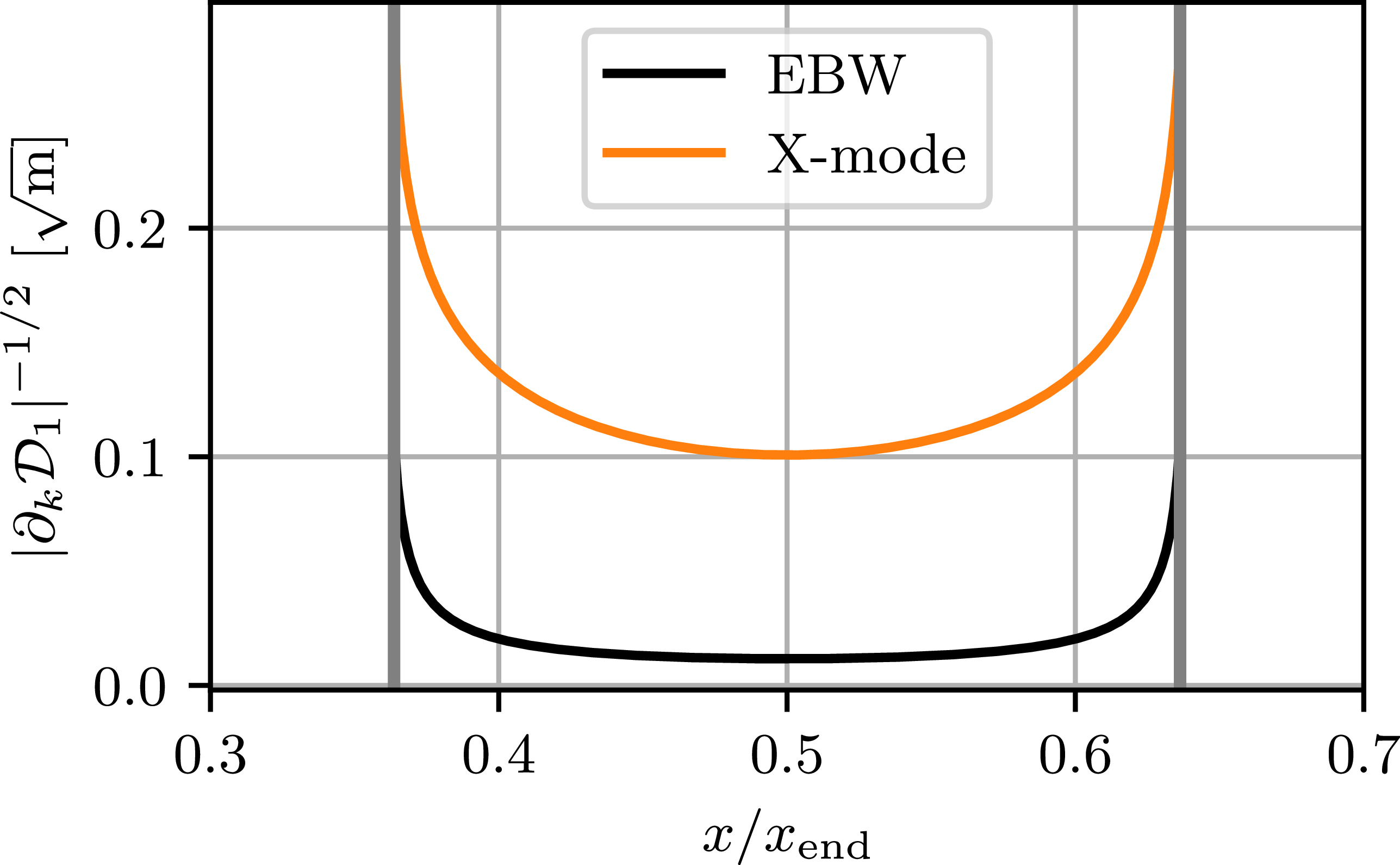
The time-independent spatial variation of the wave $\phi _1(x,t)$
for
$\phi _1(x,t)$
for $k_1$
as a function of
$k_1$
as a function of $x$
in the plasma profile. The orange line shows the values computed for the X-mode part of the wave, and the black line is the EBW part. The grey lines show the UH layers.
$x$
in the plasma profile. The orange line shows the values computed for the X-mode part of the wave, and the black line is the EBW part. The grey lines show the UH layers.

2.3.1. Spatially averaged estimation
Previous estimations of TPDI growth rates assume that the spatial variation of $\phi _1(x,t)$
is constant in time (Hansen Reference Hansen2019; Senstius et al. Reference Senstius, Gusakov, Yu Popov and Nielsen2022; Clod et al. Reference Clod, Senstius, Nielsen, Ragona, Thrysøe, Kumar, Coda and Nielsen2024; de Wit et al. Reference de Wit, Senstius, Clod, Ragona and Nielsen2025). The assumption implies that
$\phi _1(x,t)$
is constant in time (Hansen Reference Hansen2019; Senstius et al. Reference Senstius, Gusakov, Yu Popov and Nielsen2022; Clod et al. Reference Clod, Senstius, Nielsen, Ragona, Thrysøe, Kumar, Coda and Nielsen2024; de Wit et al. Reference de Wit, Senstius, Clod, Ragona and Nielsen2025). The assumption implies that $\phi _1(x,t)$
can be put on the form of
$\phi _1(x,t)$
can be put on the form of $\phi _1(x,t) = a_1(t)b_1(x)$
, where
$\phi _1(x,t) = a_1(t)b_1(x)$
, where $a_1(t)$
represents a time-dependent scaling factor to the spatial profile
$a_1(t)$
represents a time-dependent scaling factor to the spatial profile $b_1(x)$
. As in Hansen (Reference Hansen2019), a reasonable expression for
$b_1(x)$
. As in Hansen (Reference Hansen2019), a reasonable expression for $b_1(x)$
is obtained by considering the steady-state solution to the linear part of (2.15)
$b_1(x)$
is obtained by considering the steady-state solution to the linear part of (2.15)
 \begin{equation} \begin{split} &-\partial _x\phi _1(x)\partial _k\mathcal{D}_1 - \frac {1}{2}\phi _1(x)\partial _{x}\big \{\partial _k\mathcal{D}_1\big \} = 0. \end{split} \end{equation}
The equation is a dynamic equation dictating how the envelope of the wave evolves as it propagates in space. The solution to (2.16) is obtained as $\phi _1(x) = a_{0,1}b_1(x)$
,
$\phi _1(x) = a_{0,1}b_1(x)$
, $b_1(x)=1/\sqrt {\partial _k\mathcal{D}_1}$
, where the time-independent spatial variation is shown in figure 2 for both the EBW and X-mode part of the wave. It can be noted that they diverge at the UH layers with unphysically high values (Tracy et al. Reference Tracy, Brizard, Richardson and Kaufman2014). This results from a direct limitation of the WKB approximation, and may influence the estimated growth rates of the TPDI. However, the phase matching condition is not fulfilled close to the UH layers, causing the contributions of these regions to the total growth rate of the instability to therefore be small. We now describe each UH wave
$b_1(x)=1/\sqrt {\partial _k\mathcal{D}_1}$
, where the time-independent spatial variation is shown in figure 2 for both the EBW and X-mode part of the wave. It can be noted that they diverge at the UH layers with unphysically high values (Tracy et al. Reference Tracy, Brizard, Richardson and Kaufman2014). This results from a direct limitation of the WKB approximation, and may influence the estimated growth rates of the TPDI. However, the phase matching condition is not fulfilled close to the UH layers, causing the contributions of these regions to the total growth rate of the instability to therefore be small. We now describe each UH wave $1,\ 2$
as a superposition of their EBW and X-mode components, sharing a time-dependent scaling factor
$1,\ 2$
as a superposition of their EBW and X-mode components, sharing a time-dependent scaling factor $a_j(t)$
 \begin{equation} \begin{split} \varPhi _j(x,t) = a_j(t)&\left [\frac {\exp (i\theta _{j}^+)}{\sqrt {\partial _k\mathcal{D}_j^+}}+ \frac {\exp (i\theta _j^-)}{\sqrt {\partial _k\mathcal{D}_j^-}} \right ]\!. \end{split} \end{equation}
To align with the notation of earlier TPDI studies (Hansen Reference Hansen2019; Clod et al. Reference Clod, Senstius, Nielsen, Ragona, Thrysøe, Kumar, Coda and Nielsen2024), the superscript ‘ $+$
’ denotes the EBW component of the UH wave, whereas ‘
$+$
’ denotes the EBW component of the UH wave, whereas ‘ $-$
’ is the X-mode part. The envelope equation in (2.15) is re-obtained now with the WKB wave amplitude from (2.17). By multiplying the expression with
$-$
’ is the X-mode part. The envelope equation in (2.15) is re-obtained now with the WKB wave amplitude from (2.17). By multiplying the expression with
 \begin{equation} \left [\frac {\exp (-i\theta _j^+)}{\Big (\sqrt {\partial _k\mathcal{D}_j^+}\Big )^*}+\frac {\exp (-i\theta _j^-)}{\Big (\sqrt {\partial _k\mathcal{D}_j^-}\Big )^*}\right ]\!, \end{equation}
the following relation for UH wave $1$
is obtained as:
$1$
is obtained as:
 \begin{equation} i\partial _{t}a_{1}(t)\left [\frac {\partial _{\omega} \mathcal{D}_1^+}{|\partial _k\mathcal{D}_1^+|} +\frac {\partial _{\omega} \mathcal{D}_1^-}{|\partial _k\mathcal{D}_1^-|}\right ] = \frac {\rho _{\text{nl,1}}e^{-i\theta _{1}^+(x,t)}}{\varepsilon _0\big (\sqrt {\partial _k\mathcal{D}_1^{\text{+}}}\big )^*}, \end{equation}
where terms with fast phase variations have been neglected, as these are assumed to ultimately mix to zero. The nonlinearly induced charge density is further expressed in terms of a nonlinear susceptibility $\chi _{nl}$
, such that
$\chi _{nl}$
, such that $\rho _{\text{nl,1}} = E_0\varPhi _2^*\chi _{\text{nl}}\varepsilon _0$
, where
$\rho _{\text{nl,1}} = E_0\varPhi _2^*\chi _{\text{nl}}\varepsilon _0$
, where $E_0$
and
$E_0$
and $\varPhi _2$
are the WKB wave fields of the injected wave and the second UH wave, respectively. The susceptibility represents nonlinear coupling strength between the three waves, and the resulting expression in taken from Gusakov et al. (Reference Gusakov, Popov and Tretinnikov2019b
and Senstius et al. (Reference Senstius, Gusakov, Yu Popov and Nielsen2022)
$\varPhi _2$
are the WKB wave fields of the injected wave and the second UH wave, respectively. The susceptibility represents nonlinear coupling strength between the three waves, and the resulting expression in taken from Gusakov et al. (Reference Gusakov, Popov and Tretinnikov2019b
and Senstius et al. (Reference Senstius, Gusakov, Yu Popov and Nielsen2022)
 \begin{equation} \begin{split} \chi _{\text{nl}} &= \frac {1}{2B^{(0)}}\frac {\omega _{pe}^2\omega _{ce}^2\omega _0^2}{(\omega _0^2 - \omega _{ce}^2)(\bar {\omega }^2 - \omega _{ce}^2)^2}\frac {k_0k_1k_2}{4\omega _0}\\&\quad \times \left (7+3\frac {D_0}{S_0}\frac {\omega _0}{\omega _{ce}} - \frac {4\omega _{ce}^2}{\omega _0^2}\right ), \end{split} \end{equation}
where $\bar {\omega } = (\omega _1 +\omega _2)/2$
, and
$\bar {\omega } = (\omega _1 +\omega _2)/2$
, and $D_0$
and
$D_0$
and $S_0$
are the difference and sum parameters for the injected wave from (2.10). The wave field
$S_0$
are the difference and sum parameters for the injected wave from (2.10). The wave field $\varPhi _2(x,t)$
is described similarly using (2.17), and the injected X-mode wave is given as
$\varPhi _2(x,t)$
is described similarly using (2.17), and the injected X-mode wave is given as
 \begin{equation} E_0(x,t) = {E}_0\exp (i\theta _0), \end{equation}
where ${E}_0$
is the electric field amplitude of the pump wave, assumed here to be constant, as the wave interacts only weakly with the plasma. An average value is then calculated by integrating over the interaction region
${E}_0$
is the electric field amplitude of the pump wave, assumed here to be constant, as the wave interacts only weakly with the plasma. An average value is then calculated by integrating over the interaction region
 \begin{equation} \begin{split} &i\partial _t a_1(t) = \text{E}_0\frac {a_2^*(t)}{\langle \partial _\omega \mathcal{D}_1\rangle }\int _{x_l}^{x_r}\text{d}x\ \frac {\chi _{\text{nl}}\exp [i\varPsi (x)]}{\left (\sqrt {\partial _k\mathcal{D}_1^+}\right )^*\left (\sqrt {\partial _k\mathcal{D}_2^+}\right )^*}, \end{split} \end{equation}
where the exponent $\varPsi (x)$
takes into account the phase mismatch caused by the inhomogeneous medium
$\varPsi (x)$
takes into account the phase mismatch caused by the inhomogeneous medium
 \begin{equation} \varPsi (x) = \int ^x\text{d}x'\ [k_0(x') - k_1^+(x') - k_2^+(x')]. \end{equation}
The integration bounds, $x_l$
and
$x_l$
and $x_r$
, are the left and right UH layers for the innermost UH wave in figure 1, respectively. The integral represents an average gain in amplitude the daughter wave attains from the nonlinear interaction as it completes a round trip in the cavity. Finally, the value
$x_r$
, are the left and right UH layers for the innermost UH wave in figure 1, respectively. The integral represents an average gain in amplitude the daughter wave attains from the nonlinear interaction as it completes a round trip in the cavity. Finally, the value $\langle \partial \omega \mathcal{D}_1(k,\omega )\rangle$
is given as
$\langle \partial \omega \mathcal{D}_1(k,\omega )\rangle$
is given as
 \begin{equation} \begin{split} \langle \partial _\omega &\mathcal{D}_1\rangle =\int _{x_l}^{x_r}\left (\frac {\partial _\omega \mathcal{D}_1^+}{|\partial _k\mathcal{D}_1^+|} +\frac {\partial _\omega \mathcal{D}_1^-}{|\partial _k\mathcal{D}_1^-|}\right )\ \text{d}x. \end{split} \end{equation}
The evolution of $a_2(t)$
is obtained similarly to (2.22), and the system of equations can be written on the following form (Senstius et al. Reference Senstius, Gusakov, Yu Popov and Nielsen2022; Clod et al. Reference Clod, Senstius, Nielsen, Ragona, Thrysøe, Kumar, Coda and Nielsen2024):
$a_2(t)$
is obtained similarly to (2.22), and the system of equations can be written on the following form (Senstius et al. Reference Senstius, Gusakov, Yu Popov and Nielsen2022; Clod et al. Reference Clod, Senstius, Nielsen, Ragona, Thrysøe, Kumar, Coda and Nielsen2024):
 \begin{equation} i\partial _ta_1(t) = \xi _{1,2}a_2^*(t),\quad -i\partial _ta_2^*(t) = \xi _{2,1}^*a_1(t). \end{equation}
The coupled system in (2.25) may now be solved as an eigenvalue problem, yielding the growth rate of their shared exponential increase in time
 \begin{equation} a_j(t) = a_j(0)\exp (\gamma t), \quad \gamma = \sqrt {\xi _{1,2}\xi _{2,1}^*}, \end{equation}
for daughter wave $j$
. The coupling coefficients are given as
$j$
. The coupling coefficients are given as
 \begin{equation} \begin{split} \xi _{j,b} = \frac {\text{E}_0}{\langle \partial _\omega \mathcal{D}_j\rangle }\int _{x_l}^{x_r}\text{d}x\ \frac {\chi _{nl}\exp [i\varPsi\!(x)]}{\left (\sqrt {\partial _k\mathcal{D}_j^+}\right )^*\left (\sqrt {\partial _k\mathcal{D}_b^+}\right )^*}. \end{split} \end{equation}
Lastly, trapped waves must interfere constructively with themselves as they perform round trips in the cavity. Only modes whose phase attains an integer multiple of $2\pi$
after completing round trips satisfy this condition, effectively resulting in a discretised frequency spectrum of allowed eigenmodes (Senstius, Nielsen & Vann Reference Senstius, Nielsen and Vann2021). The quantisation rule is given as (Gusakov & Popov Reference Gusakov and Popov2020)
$2\pi$
after completing round trips satisfy this condition, effectively resulting in a discretised frequency spectrum of allowed eigenmodes (Senstius, Nielsen & Vann Reference Senstius, Nielsen and Vann2021). The quantisation rule is given as (Gusakov & Popov Reference Gusakov and Popov2020)
 \begin{equation} \int _{x_l}^{x_r}(|k^+| - |k^-|)\ \text{d}x = \left (2m+1\right )\pi , \end{equation}
where $m\in \mathrm{N}_0$
is the quantisation number. The added
$m\in \mathrm{N}_0$
is the quantisation number. The added $\pi$
on the right-hand side of (2.28) originates from a
$\pi$
on the right-hand side of (2.28) originates from a $\pi /2$
phase shift gained at the X-mode to EBW (or the reverse) conversion point in the profile for each individual mode, which is experienced twice during a round trip. The daughter waves of the TPDI are in this study assumed to be eigenmodes that satisfy (2.28), both with an individual mode number.
$\pi /2$
phase shift gained at the X-mode to EBW (or the reverse) conversion point in the profile for each individual mode, which is experienced twice during a round trip. The daughter waves of the TPDI are in this study assumed to be eigenmodes that satisfy (2.28), both with an individual mode number.
2.3.2. Full calculation
Instead of estimating only the average gain in growth during a round trip in the cavity, the envelopes $\phi _1(x,t)$
and
$\phi _1(x,t)$
and $\phi _2(x,t)$
may be directly evolved forward in space and time. Turning to the envelope equation in (2.15), the UH waves are again described by a superposition of their EBW and X-mode components
$\phi _2(x,t)$
may be directly evolved forward in space and time. Turning to the envelope equation in (2.15), the UH waves are again described by a superposition of their EBW and X-mode components
 \begin{equation} \varPhi _j(x,t) = \phi _j^+(x,t)e^{i\theta _j^+(x,t)}+\phi _j^-(x,t)e^{i\theta _j^-(x,t)}. \end{equation}
Isolating the time derivatives of $\phi _j(x,t)$
and neglecting terms with fast phase variations, the envelope (2.15) can be cast as two separate equations, one for the X-mode part and one for the EBW part. We start with the X-mode part that is assumed to not experience any nonlinear wave interactions. Equation (2.15) is simplified by introducing the scaled amplitude
$\phi _j(x,t)$
and neglecting terms with fast phase variations, the envelope (2.15) can be cast as two separate equations, one for the X-mode part and one for the EBW part. We start with the X-mode part that is assumed to not experience any nonlinear wave interactions. Equation (2.15) is simplified by introducing the scaled amplitude $a_j^-(x,t)$
, such that
$a_j^-(x,t)$
, such that
 \begin{equation} \phi _j^-(x,t) = \frac {a_j^-(x,t)}{\sqrt {\partial _k \mathcal{D}_j^-}}, \end{equation}
which is similar to the solution for $\phi _j(x)$
in the steady-state system in (2.16), leading to
$\phi _j(x)$
in the steady-state system in (2.16), leading to
 \begin{equation} \frac {i\partial _\omega \mathcal{D}_j^-}{\sqrt {\partial _k\mathcal{D}_j^-}}\left (\partial _t a_j^- + v_{gj}^-\partial _x a_j^-\right )=0, \end{equation}
where $v_{gj}^-=-\partial _k\mathcal{D}_{j}^-/\partial _\omega \mathcal{D}_j^-$
is the group velocity of the X-mode part. The nonlinear coupling term is introduced in the EBW part of the wave, yielding instead
$v_{gj}^-=-\partial _k\mathcal{D}_{j}^-/\partial _\omega \mathcal{D}_j^-$
is the group velocity of the X-mode part. The nonlinear coupling term is introduced in the EBW part of the wave, yielding instead
 \begin{equation} \partial _t a_j^+=- v_{gj}^+\partial _x a_j^++\varLambda _{j,b} a_b^{+*} e^{i\varPsi (x)}, \end{equation}
where the coupling strength $\varLambda _{j,b}$
is given by
$\varLambda _{j,b}$
is given by
 \begin{equation} \varLambda _{j,b} = -i\text{E}_0\frac {\chi _{nl}\sqrt {\partial _k\mathcal{D}_j^+}}{\partial _\omega \mathcal{D}_j^+\Big(\sqrt {\partial _k\mathcal{D}_b^+}\Big)^*}. \end{equation}
Equations (2.32) and (2.31) may now be computed on a spatial grid and evolved forward in time. To ensure a linear conversion between the X-mode and EBW components for each UH wave, an ad hoc term is added to both expressions, defined as $w(a_j^--a_j^+)$
. The parameter
$w(a_j^--a_j^+)$
. The parameter $w$
is positive and only non-zero at the location where the X-mode converts into its counter-propagating EBW component. It is chosen here to be located a few grid cells before the true UH layer appears. Oppositely, the expression is only non-zero and negative at the other end, where the EBW mode converts back into the X-mode again. The phase information of the daughter wave eigenmodes is precomputed and stored in
$w$
is positive and only non-zero at the location where the X-mode converts into its counter-propagating EBW component. It is chosen here to be located a few grid cells before the true UH layer appears. Oppositely, the expression is only non-zero and negative at the other end, where the EBW mode converts back into the X-mode again. The phase information of the daughter wave eigenmodes is precomputed and stored in $\varPsi (x)$
in the coupling term of (2.32). If both the X-mode and EBW components of the modes were to couple nonlinearly with the pump wave in the model, it is important to remember the
$\varPsi (x)$
in the coupling term of (2.32). If both the X-mode and EBW components of the modes were to couple nonlinearly with the pump wave in the model, it is important to remember the $\pi /2$
phase shift gained at each conversion point.
$\pi /2$
phase shift gained at each conversion point.
Due to numerical stability, the conversion term will only raise the amplitude of the other component while not draining the corresponding incoming wave. The incoming wave instead outflows the domain located between the UH layers with a fixed and finite velocity, before reaching a damping region at the ends of the total domain. The spatial derivatives are computed using either a fourth-order finite forward or backward difference scheme, to match the sign of their velocities. The differential schemes also have periodic indexing at the boundaries, creating periodic boundary conditions for small residuals of the wave field amplitudes of order $\mathcal{O}(\epsilon )$
that remain after the damping. This is done to avoid potential oscillatory behaviours from discontinuities in the amplitude gradients. Finally, the time-dependent spatial envelope profiles are evolved forward in time using a fourth-order Runge–Kutta scheme. In the absence of a pump wave field, the UH waves propagate independently with expected group velocities and conserved amplitudes after multiple round trips in the cavity.
$\mathcal{O}(\epsilon )$
that remain after the damping. This is done to avoid potential oscillatory behaviours from discontinuities in the amplitude gradients. Finally, the time-dependent spatial envelope profiles are evolved forward in time using a fourth-order Runge–Kutta scheme. In the absence of a pump wave field, the UH waves propagate independently with expected group velocities and conserved amplitudes after multiple round trips in the cavity.
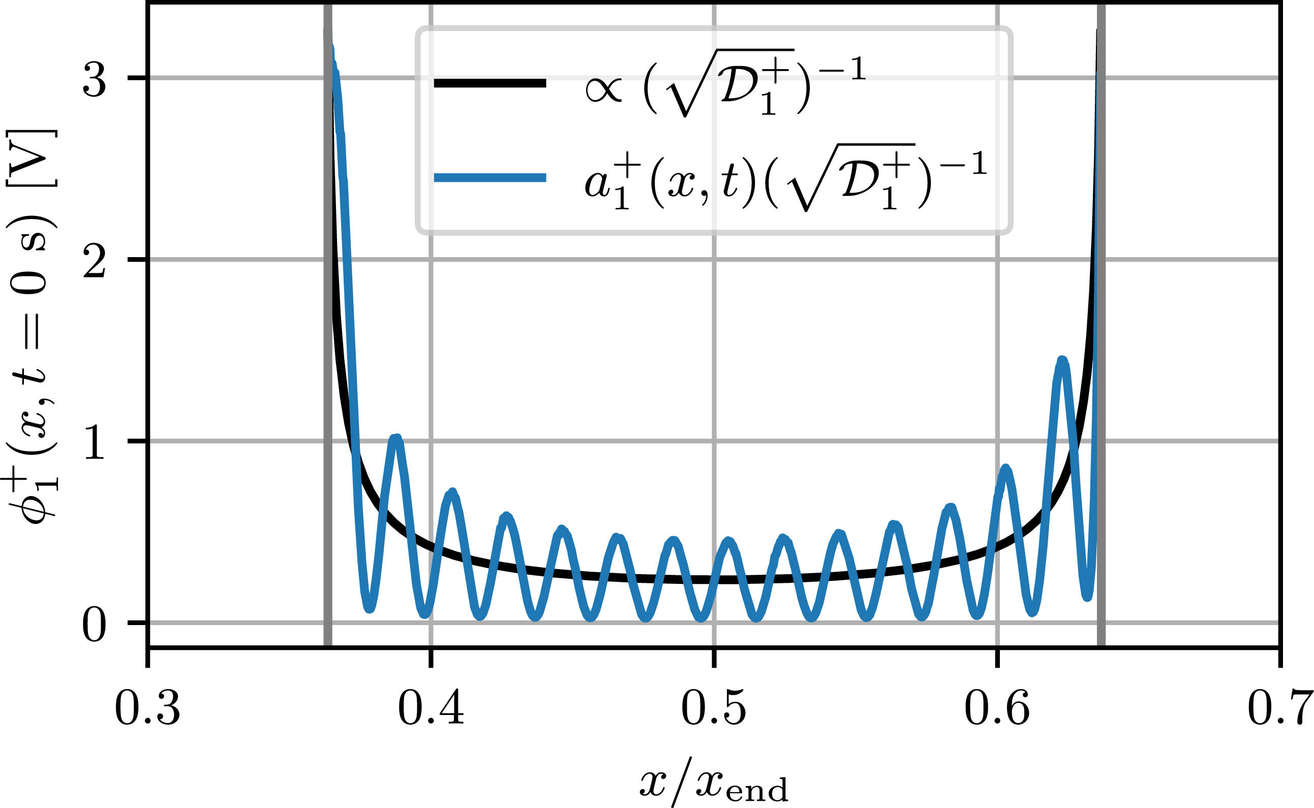
The initial profile of $\phi _1^{+}(x,t)$
at time
$\phi _1^{+}(x,t)$
at time $t=0\,\mathrm{s}$
, plotted as the blue line. The black line shows the profile, implied by the separation of variables for the spatially averaged model. The grey lines mark the UH layers.
$t=0\,\mathrm{s}$
, plotted as the blue line. The black line shows the profile, implied by the separation of variables for the spatially averaged model. The grey lines mark the UH layers.

Both $a_1^+(x,t)$
and
$a_1^+(x,t)$
and $a_2^+(x,t)$
are initialised on the spatial grid with baseline values and a randomised phase, while also being seeded with small-scale noise and a sinusoidal pattern to emulate potential inhomogeneities. Their X-mode counterparts have the same baseline values with only noise added. The initial conditions for
$a_2^+(x,t)$
are initialised on the spatial grid with baseline values and a randomised phase, while also being seeded with small-scale noise and a sinusoidal pattern to emulate potential inhomogeneities. Their X-mode counterparts have the same baseline values with only noise added. The initial conditions for $\phi _1^+(x,t)$
can be seen in figure 3. The wave field
$\phi _1^+(x,t)$
can be seen in figure 3. The wave field $\phi _2^+$
is excluded in the plot for visual clarity, but it looks similar as well.
$\phi _2^+$
is excluded in the plot for visual clarity, but it looks similar as well.
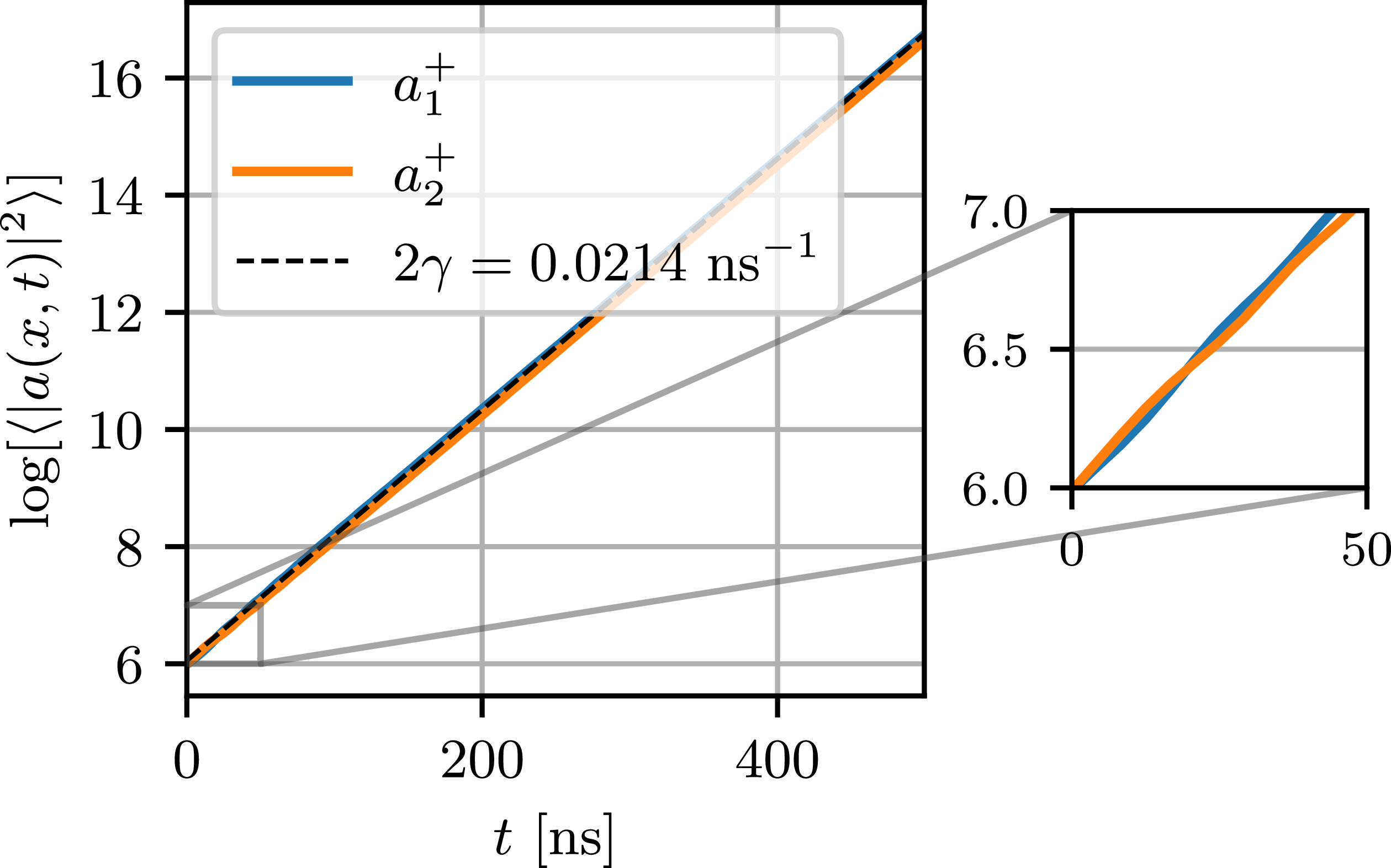
The spatial mean of the power of each wave’s envelope profile plotted as a function of time in logarithmic values. The dashed black line shows the numerical fit that is computed with the measured growth rate.

The constant amplitude of the injected X-mode wave is defined through the intensity of a plane wave in vacuum, $\text{E}_0 = \sqrt {2I_0/(c\varepsilon _0)}$
, where
$\text{E}_0 = \sqrt {2I_0/(c\varepsilon _0)}$
, where $I_0=1\,\mathrm{kW\,cm}^{-2}$
is a fixed intensity. The growth rate of the instability is measured by computing the spatial mean between the UH layers of each wave, shown in figure 4. A linear fit on the form
$I_0=1\,\mathrm{kW\,cm}^{-2}$
is a fixed intensity. The growth rate of the instability is measured by computing the spatial mean between the UH layers of each wave, shown in figure 4. A linear fit on the form $y = 2m_1\ t+m_2$
is computed for the logarithmic values of
$y = 2m_1\ t+m_2$
is computed for the logarithmic values of $a_1^+(x,t)$
, yielding
$a_1^+(x,t)$
, yielding $2m_1 =(2.14\pm 0.02)\times 10^{-2}\,\mathrm{ns}^{-1}$
. For comparison, the spatially averaged method estimates a growth rate of
$2m_1 =(2.14\pm 0.02)\times 10^{-2}\,\mathrm{ns}^{-1}$
. For comparison, the spatially averaged method estimates a growth rate of $2\gamma =2.11\times 10^{-2}\,\mathrm{ns^{-1}}$
, which lies close in value. It is also noted that the growths in figure 4 fluctuate at early times (
$2\gamma =2.11\times 10^{-2}\,\mathrm{ns^{-1}}$
, which lies close in value. It is also noted that the growths in figure 4 fluctuate at early times ( $t\lt 300\,\mathrm{ns}$
) due to the initial inhomogeneities. A zoom-in of this is highlighted in the figure. However, after the transient period (
$t\lt 300\,\mathrm{ns}$
) due to the initial inhomogeneities. A zoom-in of this is highlighted in the figure. However, after the transient period ( $t\gt 300\,\mathrm{ns}$
) their increments become steady, suggesting that the envelopes converge toward the expected form
$t\gt 300\,\mathrm{ns}$
) their increments become steady, suggesting that the envelopes converge toward the expected form $\phi _j(x,t) = a_j(t)b_j(x)$
. To further assess this,
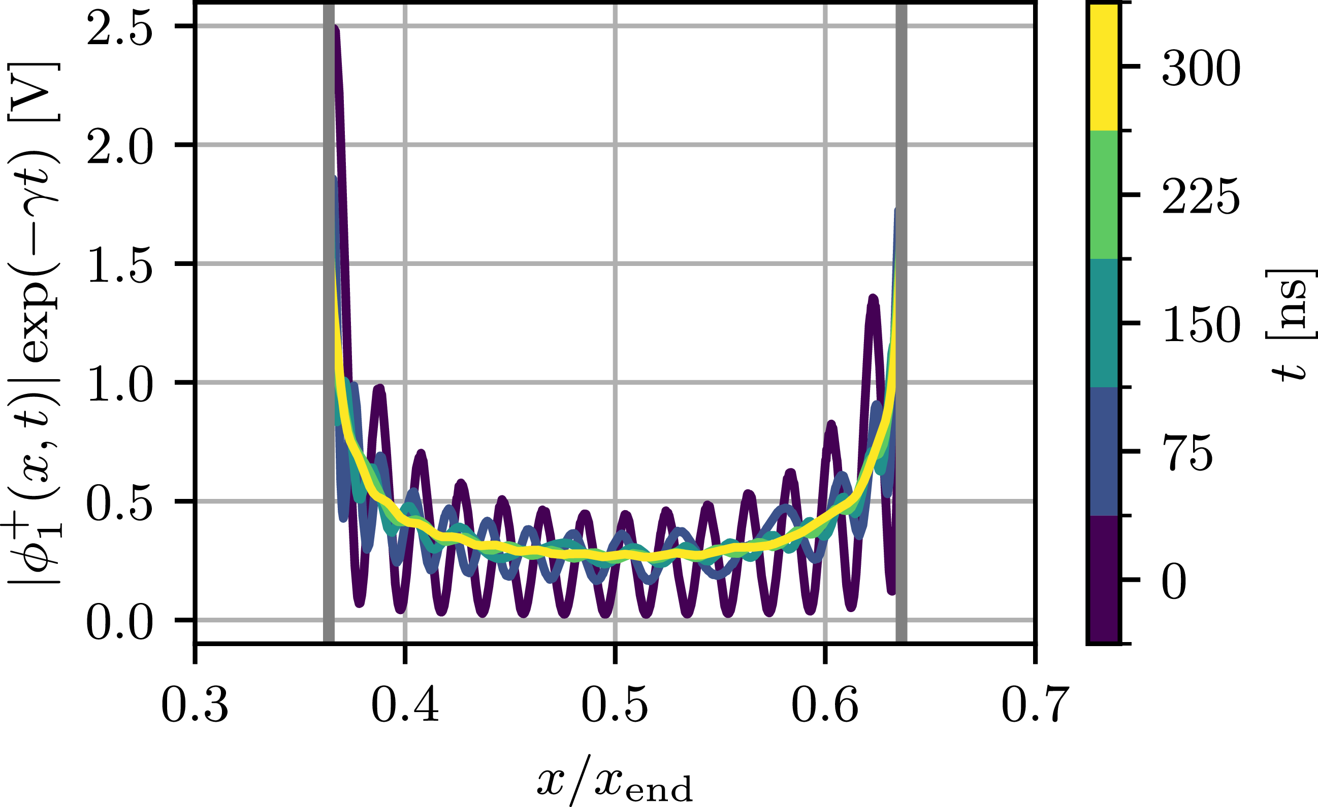
$\phi _j(x,t) = a_j(t)b_j(x)$
. To further assess this, $\phi _1^+(x, t_i)$
is plotted in figure 5 at five different time instances,
$\phi _1^+(x, t_i)$
is plotted in figure 5 at five different time instances, $t_i\in \{0, 75, 150, 225, 300\}\ \text{ns}$
, where the values are normalised by the exponential growth from the instability. It is seen that the instability drives
$t_i\in \{0, 75, 150, 225, 300\}\ \text{ns}$
, where the values are normalised by the exponential growth from the instability. It is seen that the instability drives $\phi _1^+$
toward a smooth, steady-state profile, scaled by the exponential growth factor
$\phi _1^+$
toward a smooth, steady-state profile, scaled by the exponential growth factor $\exp (\gamma t)$
. In other words, noise and inhomogeneities from the initial profile are evened out, and the full solution asymptotically satisfies the separation of variables assumption. This asymptotic convergence has been further verified by applying various initial conditions for the envelopes, including cases that deviate significantly from
$\exp (\gamma t)$
. In other words, noise and inhomogeneities from the initial profile are evened out, and the full solution asymptotically satisfies the separation of variables assumption. This asymptotic convergence has been further verified by applying various initial conditions for the envelopes, including cases that deviate significantly from $\propto (\sqrt {\mathcal{D}_j})^{-1}$
. In all cases, similar spatial profiles of
$\propto (\sqrt {\mathcal{D}_j})^{-1}$
. In all cases, similar spatial profiles of $\phi _1^+$
and
$\phi _1^+$
and $\phi _2^+$
were reached after approximately
$\phi _2^+$
were reached after approximately $300\,\mathrm{ns}$
. Reducing the coupling strength by a factor of three extended the transient period to approximately
$300\,\mathrm{ns}$
. Reducing the coupling strength by a factor of three extended the transient period to approximately $900\,\mathrm{ns}$
. These results imply that the spatially averaged model can be reliably applied after time scales of roughly
$900\,\mathrm{ns}$
. These results imply that the spatially averaged model can be reliably applied after time scales of roughly $10/(2\gamma )$
, provided that secondary decay processes have not yet impacted
$10/(2\gamma )$
, provided that secondary decay processes have not yet impacted $\phi _1^+$
and
$\phi _1^+$
and $\phi _2^+$
locally within the domain.
$\phi _2^+$
locally within the domain.
The envelope $\phi ^+_1(x,t)$
plotted as a function of position for multiple times instances. The values are divided by the exponential growth
$\phi ^+_1(x,t)$
plotted as a function of position for multiple times instances. The values are divided by the exponential growth $\exp (\gamma t)$
.
$\exp (\gamma t)$
.

3. Conclusion
We have investigated the validity of a spatially averaged TPDI model for estimating the exponential growth of two trapped UH waves that couple to an injected X-mode polarised wave. The model describes the UH waves by an envelope equation, derived from classical WKB methods, and assumes a separation of variables between the temporal and spatial parts of the wave fields. Based on this, the spatially averaged gain and the total growth rate in the linear regime of the instability can be computed.
To test this assumption, we directly modelled the UH waves on a spatial grid and evolved them in time using a fourth-order Runge–Kutta scheme. We found that initially imposed inhomogeneities in the field amplitudes were smoothed out by the instability, which drove the amplitudes toward a time-independent spatial profile scaled by an exponential growth factor. This relaxation occurred over a transient period of roughly $300\,\mathrm{ns}$
. In general, convergence to the steady-state profile was achieved after approximately
$300\,\mathrm{ns}$
. In general, convergence to the steady-state profile was achieved after approximately $10/(2\gamma )\,\mathrm{ns}$
, independent of the initial shape of the field amplitudes. An exponential fit to the UH wave growth yielded a rate of
$10/(2\gamma )\,\mathrm{ns}$
, independent of the initial shape of the field amplitudes. An exponential fit to the UH wave growth yielded a rate of $(2.14\pm 0.02)\times 10^{-2}\,\mathrm{ns^{-1}}$
, in close agreement with the spatially averaged prediction of
$(2.14\pm 0.02)\times 10^{-2}\,\mathrm{ns^{-1}}$
, in close agreement with the spatially averaged prediction of $2.11\times 10^{-2}\,\mathrm{ns^{-1}}$
. This demonstrates that the spatially averaged model is asymptotically valid.
$2.11\times 10^{-2}\,\mathrm{ns^{-1}}$
. This demonstrates that the spatially averaged model is asymptotically valid.
In conclusion, the results show that the spatially averaged model provides an accurate estimate of the growth rate for the one-dimensional two-plasmon decay instability. The newly developed spatio-temporal method also enables modelling of additional parametric interactions with escaping waves, for instance secondary parametric saturation processes of the instability.
Acknowledgements
This work has been funded by Novo Nordisk Fonden, NNF22OC0076017, and the Carlsberg Foundation grant, CF23-0181. This work has been carried out within the framework of the EUROfusion Consortium, funded by the European Union via the Euratom Research and Training Programme (Grant Agreement No 101052200 -EUROfusion). Views and opinions expressed are, however, those of the author(s) only and do not necessarily reflect those of the European Union or the European Commission. Neither the European Union nor the European Commission can be held responsible for them.
Editor Paolo Ricci thanks the referees for their advice in evaluating this article.
Data availability statement
All data that support the findings of this study are included within the article (and any supplementary files).
Declaration of interests
The authors report no conflicts of interest.


 Open access