


1. Introduction
Turbulent flows play a crucial role in the transport of thermal energy and physical matter within fluid flows since their chaotic motions promote enhanced interlayer mixing compared with laminar flow, where the differences in their thermal or matter transport can be encapsulated within the molecular Prandtl number ( $ \textit{Pr} = \nu / \alpha$
), the ratio between kinematic viscosity (
$ \textit{Pr} = \nu / \alpha$
), the ratio between kinematic viscosity ( $\nu$
) and the thermal diffusivity (
$\nu$
) and the thermal diffusivity ( $\alpha$
), and the Schmidt number (
$\alpha$
), and the Schmidt number ( $ \textit{Sc} = \nu / D$
), the ratio between the kinematic viscosity and the mass diffusivity (
$ \textit{Sc} = \nu / D$
), the ratio between the kinematic viscosity and the mass diffusivity ( $D$
). Physical understanding of flows with heat transfer or mass transport at
$D$
). Physical understanding of flows with heat transfer or mass transport at $ \textit{Pr}$
,
$ \textit{Pr}$
, $ \textit{Sc} \approx 1$
is obvious since the velocity behaviour will be identical to the temperature or contaminant behaviours, but in reality, different flow media exhibit a wide range of
$ \textit{Sc} \approx 1$
is obvious since the velocity behaviour will be identical to the temperature or contaminant behaviours, but in reality, different flow media exhibit a wide range of $ \textit{Pr}$
and
$ \textit{Pr}$
and $ \textit{Sc}$
. Commonplace fluids in engineering, such as water, engine oils, glycerol and polymer melts, have significantly higher
$ \textit{Sc}$
. Commonplace fluids in engineering, such as water, engine oils, glycerol and polymer melts, have significantly higher $ \textit{Pr}$
than 1 (Pirozzoli Reference Pirozzoli2023b
), whereas low and very low
$ \textit{Pr}$
than 1 (Pirozzoli Reference Pirozzoli2023b
), whereas low and very low $ \textit{Pr}$
flows are important in the simulation of nuclear liquid metal reactors and concentrated solar power technologies (Cachafeiro et al. Reference Cachafeiro, Arevalo, Vinuesa, Goikoetxea and Barriga2015). The emergence of stellar fluid dynamics and its related data has also motivated further research into asymptotically small
$ \textit{Pr}$
flows are important in the simulation of nuclear liquid metal reactors and concentrated solar power technologies (Cachafeiro et al. Reference Cachafeiro, Arevalo, Vinuesa, Goikoetxea and Barriga2015). The emergence of stellar fluid dynamics and its related data has also motivated further research into asymptotically small $ \textit{Pr}$
flow (Garaud Reference Garaud2018, Reference Garaud2021). In practice,
$ \textit{Pr}$
flow (Garaud Reference Garaud2018, Reference Garaud2021). In practice, $ \textit{Sc}$
is also typically much greater than 1 for the diffusion of contaminants. Therefore, the relationship between momentum transfer and passive scalar transfer has always received considerable attention across all flow regimes, particularly, how to relate the mean streamwise velocity and temperature profiles in turbulence. Our focus in the following will be on heat transfer, but note that the study and its discussions hereafter could also be applied to the diffusion of contaminants by replacing
$ \textit{Sc}$
is also typically much greater than 1 for the diffusion of contaminants. Therefore, the relationship between momentum transfer and passive scalar transfer has always received considerable attention across all flow regimes, particularly, how to relate the mean streamwise velocity and temperature profiles in turbulence. Our focus in the following will be on heat transfer, but note that the study and its discussions hereafter could also be applied to the diffusion of contaminants by replacing $ \textit{Pr}$
with
$ \textit{Pr}$
with $ \textit{Sc}$
and other thermal-related quantities with mass-diffusivity equivalents.
$ \textit{Sc}$
and other thermal-related quantities with mass-diffusivity equivalents.
These variations in the flow parameter, $ \textit{Pr}$
, have led to numerous difficulties in finding a universal scaling regarding temperatures and, therefore, the modelling of it. In particular, its relationship with its velocity counterpart has received considerable attention, which is broadly referred to as the Reynolds analogy (Reynolds Reference Reynolds1874). Mean velocity profiles have long exhibited strong universality with the well-established law of the wall for incompressible flows across Reynolds numbers (Prandtl Reference Prandtl1925; von Kármán Reference von Kármán1930)
$ \textit{Pr}$
, have led to numerous difficulties in finding a universal scaling regarding temperatures and, therefore, the modelling of it. In particular, its relationship with its velocity counterpart has received considerable attention, which is broadly referred to as the Reynolds analogy (Reynolds Reference Reynolds1874). Mean velocity profiles have long exhibited strong universality with the well-established law of the wall for incompressible flows across Reynolds numbers (Prandtl Reference Prandtl1925; von Kármán Reference von Kármán1930)
 \begin{align} u^+ = \frac {1}{\kappa } \ln y^+ + C, \end{align}
where $u$
is the mean streamwise velocity,
$u$
is the mean streamwise velocity, $y$
is the wall-normal coordinate,
$y$
is the wall-normal coordinate, $\kappa \approx 0.4$
is the von Kármán constant and the second constant
$\kappa \approx 0.4$
is the von Kármán constant and the second constant $C \approx 5$
. The superscript
$C \approx 5$
. The superscript $^+$
here denotes viscous scaling, such that
$^+$
here denotes viscous scaling, such that $u^+ = u / u_\tau$
and
$u^+ = u / u_\tau$
and $y^+ = y u_\tau / \nu$
, where
$y^+ = y u_\tau / \nu$
, where $u_\tau$
is the friction velocity. Borrowing this concept for temperature profiles, a similar thermal law of the wall was developed
$u_\tau$
is the friction velocity. Borrowing this concept for temperature profiles, a similar thermal law of the wall was developed
 \begin{align} \varTheta ^+ = \frac {1}{\kappa _t} \ln y^+ + B, \end{align}
where $\varTheta = T_w - T$
is the difference between the mean wall temperature and the mean temperature at a given wall-normal position. Similar to
$\varTheta = T_w - T$
is the difference between the mean wall temperature and the mean temperature at a given wall-normal position. Similar to $\kappa$
,
$\kappa$
, $\kappa _t$
is the thermal von Kármán constant, whereas, unlike (1.1),
$\kappa _t$
is the thermal von Kármán constant, whereas, unlike (1.1), $B$
is not a constant for all flow parameters but is rather
$B$
is not a constant for all flow parameters but is rather $ \textit{Pr}$
-dependent (Alcántara-Ávila et al. Reference Alcántara-Ávila, Hoyas and Pérez-Quiles2018; Alcántara-Ávila & Hoyas Reference Alcántara-Ávila, Hoyas and Pérez-Quiles2021). The universality of
$ \textit{Pr}$
-dependent (Alcántara-Ávila et al. Reference Alcántara-Ávila, Hoyas and Pérez-Quiles2018; Alcántara-Ávila & Hoyas Reference Alcántara-Ávila, Hoyas and Pérez-Quiles2021). The universality of $\kappa _t$
is also not as evident compared with its velocity counterpart when considering thermal flows with different
$\kappa _t$
is also not as evident compared with its velocity counterpart when considering thermal flows with different $ \textit{Pr}$
. Viscous scaling for the temperature difference is
$ \textit{Pr}$
. Viscous scaling for the temperature difference is $\varTheta ^+ = (T_w - T) / \varTheta _\tau$
, where
$\varTheta ^+ = (T_w - T) / \varTheta _\tau$
, where $ \varTheta _\tau = q_w / (\rho _w c_p u_\tau )$
is the friction temperature with
$ \varTheta _\tau = q_w / (\rho _w c_p u_\tau )$
is the friction temperature with $\rho _w$
,
$\rho _w$
, $c_p$
,
$c_p$
, $q_w$
, representing the fluid density at the wall, the specific heat at constant pressure and the wall heat flux,
$q_w$
, representing the fluid density at the wall, the specific heat at constant pressure and the wall heat flux, $\displaystyle q_w = k ( {{\rm d}\varTheta }/{{\rm d}y}) |_w$
, with
$\displaystyle q_w = k ( {{\rm d}\varTheta }/{{\rm d}y}) |_w$
, with $k$
as the molecular conductivity, respectively. We further note that, in the near-wall region (
$k$
as the molecular conductivity, respectively. We further note that, in the near-wall region ( $y^+ \lt 5$
, or the viscous sublayer), the scaled mean velocity profiles are identical to the scaled wall-normal coordinates, i.e.
$y^+ \lt 5$
, or the viscous sublayer), the scaled mean velocity profiles are identical to the scaled wall-normal coordinates, i.e. $u^+ = y^+$
, but this relationship must be further modified for its thermal counterpart via the Prandtl number as
$u^+ = y^+$
, but this relationship must be further modified for its thermal counterpart via the Prandtl number as $\varTheta ^+ = \textit{Pr} y^+$
, which corresponds to the conductive sublayer within the thermal boundary layer. Despite contention as to whether (1.1) and (1.2) are merely empirical (Xu & Yang Reference Xu and Yang2018; Ali & Dey Reference Ali and Dey2020), these laws are of vital importance and are cornerstones within turbulence modelling as a point of verification; models that are able to replicate these trends are generally seen as reliable, such as wall functions for Reynolds-averaged Navier–Stokes closure models or mixing length models in large-eddy simulation wall models (Spalart & Allmaras Reference Spalart and Allmaras1992; Bose & Park Reference Bose and Park2018).
$\varTheta ^+ = \textit{Pr} y^+$
, which corresponds to the conductive sublayer within the thermal boundary layer. Despite contention as to whether (1.1) and (1.2) are merely empirical (Xu & Yang Reference Xu and Yang2018; Ali & Dey Reference Ali and Dey2020), these laws are of vital importance and are cornerstones within turbulence modelling as a point of verification; models that are able to replicate these trends are generally seen as reliable, such as wall functions for Reynolds-averaged Navier–Stokes closure models or mixing length models in large-eddy simulation wall models (Spalart & Allmaras Reference Spalart and Allmaras1992; Bose & Park Reference Bose and Park2018).
Despite the similar logarithmic scaling of the velocity and temperature profiles, at more extreme Prandtl numbers, the profiles are distinctly different in scale and even shape. For example, at lower $ \textit{Pr}$
, this logarithmic scaling for the temperature profiles does not apply. Pirozzoli (Reference Pirozzoli2023b
) found that, until the friction Péclet number,
$ \textit{Pr}$
, this logarithmic scaling for the temperature profiles does not apply. Pirozzoli (Reference Pirozzoli2023b
) found that, until the friction Péclet number, $ Pe_\tau = \textit{Pr} Re_\tau$
, exceeds or equals 10.9, a thermal logarithmic region will not be present. Lastly, the simultaneous measurements of momentum-related statistics and thermal-related statistics, such as the Reynolds shear stress and wall-normal turbulent heat flux, particularly close to the wall (Araya & Castillo Reference Araya and Castillo2012), have limited accuracy and have led to data exhibiting significant scatter within different experimental studies, culminating in the reporting of differing profiles in the past (see Blom Reference Blom1970; Antonia Reference Antonia1980; Kays & Crawford Reference Kays and Crawford1993). The measurement of either statistic only is more preferable and reliable, and as such, a more general relationship between velocity and temperature has been sought after, especially to account for the variation in fluid media, i.e. the changes in
$ Pe_\tau = \textit{Pr} Re_\tau$
, exceeds or equals 10.9, a thermal logarithmic region will not be present. Lastly, the simultaneous measurements of momentum-related statistics and thermal-related statistics, such as the Reynolds shear stress and wall-normal turbulent heat flux, particularly close to the wall (Araya & Castillo Reference Araya and Castillo2012), have limited accuracy and have led to data exhibiting significant scatter within different experimental studies, culminating in the reporting of differing profiles in the past (see Blom Reference Blom1970; Antonia Reference Antonia1980; Kays & Crawford Reference Kays and Crawford1993). The measurement of either statistic only is more preferable and reliable, and as such, a more general relationship between velocity and temperature has been sought after, especially to account for the variation in fluid media, i.e. the changes in $ \textit{Pr}$
or
$ \textit{Pr}$
or $ \textit{Sc}$
. Considering the fragility and heavy
$ \textit{Sc}$
. Considering the fragility and heavy $ \textit{Pr}$
-dependence of (1.2), especially its diminishing resemblance to the velocity profile with variations in
$ \textit{Pr}$
-dependence of (1.2), especially its diminishing resemblance to the velocity profile with variations in $ \textit{Pr}$
, a new relationship between the two quantities that can encompass a broad spectrum of prevalent engineering flow media is of significant practicality and can further the modelling and understanding of these flows.
$ \textit{Pr}$
, a new relationship between the two quantities that can encompass a broad spectrum of prevalent engineering flow media is of significant practicality and can further the modelling and understanding of these flows.
The rest of this paper is organised as follows. In § 2, a brief review of the existing modelling attempts of the temperature profiles for different $ \textit{Pr}$
is presented. We further explore the need for developing a novel temperature–velocity (TV) relationship in a more general sense with regard to the variation of
$ \textit{Pr}$
is presented. We further explore the need for developing a novel temperature–velocity (TV) relationship in a more general sense with regard to the variation of $ \textit{Pr}$
and the motivation for the current study in this section. This is followed by a description of the direct numerical simulation (DNS) data used throughout this study in § 3. In § 4, the proposed TV relationship framework, applicable for an extensive range of
$ \textit{Pr}$
and the motivation for the current study in this section. This is followed by a description of the direct numerical simulation (DNS) data used throughout this study in § 3. In § 4, the proposed TV relationship framework, applicable for an extensive range of $ \textit{Pr}$
, is introduced, with the resulting mean temperature profile reconstructions in channel and boundary layer flows shown in §§ 5 and 6, respectively. A recapitulative discussion on the model closes out the paper in § 7.
$ \textit{Pr}$
, is introduced, with the resulting mean temperature profile reconstructions in channel and boundary layer flows shown in §§ 5 and 6, respectively. A recapitulative discussion on the model closes out the paper in § 7.
2. Existing methodologies
The development of quantitative relationships between the kinetic and thermal quantities has had a lengthy history. Reynolds (Reference Reynolds1874) first developed an analogy between the two based on the similarity of the Reynolds-averaged momentum and energy transport equations in wall-bounded turbulent flows, but this was restricted to flows with Prandtl numbers close to unity. As mentioned, since, in practice, engineering fluids cover a wide range of Prandtl numbers, further studies on the effect of $ \textit{Pr}$
on the similarities and differences of velocity and passive scalars have received considerable attention (Kim, Moin & Moser Reference Kim, Moin and Moser1987; Lyons, Hanratty & McLaughlin Reference Lyons, Hanratty and McLaughlin1991; Abe & Antonia Reference Abe and Antonia2009a
; Abe, Antonia & Kawamura Reference Abe, Antonia and Kawamura2009; Pirozzoli, Bernardini & Orlandi Reference Pirozzoli, Bernardini and Orlandi2016; Abe & Antonia Reference Abe and Antonia2017). Other attempts in modelling the mean temperature profiles or relating the momentum and thermal terms have been through the turbulent Prandtl number,
$ \textit{Pr}$
on the similarities and differences of velocity and passive scalars have received considerable attention (Kim, Moin & Moser Reference Kim, Moin and Moser1987; Lyons, Hanratty & McLaughlin Reference Lyons, Hanratty and McLaughlin1991; Abe & Antonia Reference Abe and Antonia2009a
; Abe, Antonia & Kawamura Reference Abe, Antonia and Kawamura2009; Pirozzoli, Bernardini & Orlandi Reference Pirozzoli, Bernardini and Orlandi2016; Abe & Antonia Reference Abe and Antonia2017). Other attempts in modelling the mean temperature profiles or relating the momentum and thermal terms have been through the turbulent Prandtl number, $ \textit{Pr}_t$
, which is the ratio between the momentum and thermal eddy diffusivities (see Cebeci & Bradshaw Reference Cebeci and Bradshaw1988; Antonia & Kim Reference Antonia and Kim1991; Kays & Crawford Reference Kays and Crawford1993; Kays Reference Kays1994; Weigand, Ferguson & Crawford Reference Weigand, Ferguson and Crawford1997). For example, Abe & Antonia (Reference Abe and Antonia2019) proposed a quadratic fit for
$ \textit{Pr}_t$
, which is the ratio between the momentum and thermal eddy diffusivities (see Cebeci & Bradshaw Reference Cebeci and Bradshaw1988; Antonia & Kim Reference Antonia and Kim1991; Kays & Crawford Reference Kays and Crawford1993; Kays Reference Kays1994; Weigand, Ferguson & Crawford Reference Weigand, Ferguson and Crawford1997). For example, Abe & Antonia (Reference Abe and Antonia2019) proposed a quadratic fit for $ \textit{Pr}_t$
which was applicable in the outer regions of air (
$ \textit{Pr}_t$
which was applicable in the outer regions of air ( $ \textit{Pr} = 0.71$
), but does not work for mercury (
$ \textit{Pr} = 0.71$
), but does not work for mercury ( $ \textit{Pr} = 0.025$
), the other flow medium considered in the study. However, many of the studies were limited in their scope, in particular, their applicability for a large range of
$ \textit{Pr} = 0.025$
), the other flow medium considered in the study. However, many of the studies were limited in their scope, in particular, their applicability for a large range of $ \textit{Pr}$
, or were targeted for particular sections of the wall-normal profile, due to the lack of availability of data.
$ \textit{Pr}$
, or were targeted for particular sections of the wall-normal profile, due to the lack of availability of data.
2.1. Adaptation of the Johnson–King model (Pirozzoli Reference Pirozzoli2023b )
Moving away from relationships to the velocity-related quantities, and with the development of a much more comprehensive database of turbulent thermal statistics over a wide range of $ \textit{Pr}$
, Pirozzoli (Reference Pirozzoli2023b
) adapted a method from Johnson & King (Reference Johnson and King1985) to develop a model for the mean temperature profiles via the thermal eddy diffusivity,
$ \textit{Pr}$
, Pirozzoli (Reference Pirozzoli2023b
) adapted a method from Johnson & King (Reference Johnson and King1985) to develop a model for the mean temperature profiles via the thermal eddy diffusivity, $\alpha _t$
, which is expressed as follows:
$\alpha _t$
, which is expressed as follows:
 \begin{align} \alpha _t = \frac {-\overline {v'\varTheta '}}{\displaystyle \frac {{\rm d}\varTheta }{{\rm d}y}}, \end{align}
where $v$
is the wall-normal velocity, the overbar
$v$
is the wall-normal velocity, the overbar $\overline {(\boldsymbol{\cdot })}$
denotes Reynolds-averaging and
$\overline {(\boldsymbol{\cdot })}$
denotes Reynolds-averaging and $'$
denotes fluctuations from Reynolds averaging, since this allows closures of the heat fluxes with respect to the mean temperature gradient (Cebeci & Bradshaw Reference Cebeci and Bradshaw1988). This enables us to express the mean total heat fluxes as follows (Alcántara-Ávila et al. Reference Alcántara-Ávila, Hoyas and Pérez-Quiles2018):
$'$
denotes fluctuations from Reynolds averaging, since this allows closures of the heat fluxes with respect to the mean temperature gradient (Cebeci & Bradshaw Reference Cebeci and Bradshaw1988). This enables us to express the mean total heat fluxes as follows (Alcántara-Ávila et al. Reference Alcántara-Ávila, Hoyas and Pérez-Quiles2018):
 \begin{align} {q^+ = \underbrace {k^+\frac {{\rm d}\varTheta ^+}{{\rm d}y^+}}_{\text{Molecular}} \underbrace {- \overline {v'^+\varTheta '^+}}_{\text{Turbulent}} = \left (\frac {1}{ Pr} + \alpha ^+_t\right )\frac {{\rm d}\varTheta ^+}{{\rm d}y^+},} \end{align}
where $\displaystyle k^+ = {1}/\textit{Pr}$
. We note that, since properties such as density and specific heat capacity are constant, they need not be included here nor in the equations that follow. Given
$\displaystyle k^+ = {1}/\textit{Pr}$
. We note that, since properties such as density and specific heat capacity are constant, they need not be included here nor in the equations that follow. Given $q^+$
and a suitable model for
$q^+$
and a suitable model for $\alpha ^+_t$
, rearranging (2.2) gives us the thermal gradient
$\alpha ^+_t$
, rearranging (2.2) gives us the thermal gradient
 \begin{align} \frac {{\rm d}\varTheta ^+}{{\rm d}y^+} = \frac {q^+}{k^+ + \alpha _t^+}, \end{align}
and we can solve for the mean thermal profiles via integration. Pirozzoli (Reference Pirozzoli2023b
), borrowing the functional expression from Johnson & King (Reference Johnson and King1985), therefore directly modelled $\alpha _t^+$
 \begin{align} \alpha _{t, {JK}}^+ = \kappa _t y^+ D(y^+), \end{align}
where $D(y^+)$
is a damping function with asymptotic behaviours of the form
$D(y^+)$
is a damping function with asymptotic behaviours of the form
 \begin{align} D(y^+) = \left [1 - \exp \left ( -\frac {y^+}{A_\theta } \right )\right ]^2 \!, \end{align}
and the parameter $A_\theta$
is found to be 19.2 (Pirozzoli Reference Pirozzoli2023b
). We note that the thermal von Kármán constant,
$A_\theta$
is found to be 19.2 (Pirozzoli Reference Pirozzoli2023b
). We note that the thermal von Kármán constant, $\kappa _t$
, previously used for the thermal law of the wall (1.2), is utilised again in (2.4), where its value is taken as
$\kappa _t$
, previously used for the thermal law of the wall (1.2), is utilised again in (2.4), where its value is taken as $0.459$
(Pirozzoli Reference Pirozzoli2023b
). Further scrutiny of the parameters
$0.459$
(Pirozzoli Reference Pirozzoli2023b
). Further scrutiny of the parameters $A_\theta$
and
$A_\theta$
and $\kappa _t$
is provided in Appendix A, indicating that the use of the aforementioned parameter values is robust within the data used here as well. For incompressible channel and pipe turbulent flows, the total heat flux profiles,
$\kappa _t$
is provided in Appendix A, indicating that the use of the aforementioned parameter values is robust within the data used here as well. For incompressible channel and pipe turbulent flows, the total heat flux profiles, $q^+$
, can be directly derived through the integration of the thermal energy balance equations (Alcántara-Ávila et al. Reference Alcántara-Ávila, Hoyas and Pérez-Quiles2018; Pirozzoli Reference Pirozzoli2023b
), such that the Johnson–King (JK) model for the mean temperature can be found as follows:
$q^+$
, can be directly derived through the integration of the thermal energy balance equations (Alcántara-Ávila et al. Reference Alcántara-Ávila, Hoyas and Pérez-Quiles2018; Pirozzoli Reference Pirozzoli2023b
), such that the Johnson–King (JK) model for the mean temperature can be found as follows:
 \begin{align} \varTheta ^+_{\textit{JK}}(y^+) = \int ^{y^+}_0 \left (\frac {{\rm d}\varTheta ^+}{{\rm d}y^+}\right )_{\textit{JK}} \hspace {-0.1em}{\rm d}y^+ = \int ^{y^+}_0 \frac {q^+}{k^+ + \kappa _t y^+ D(y^+)}\hspace {0.2em}{\rm d}y^+. \end{align}
While the JK model (2.6) has been shown to perform relatively well for most $ \textit{Pr}$
, its direct modelling of the thermal eddy diffusivity via empirical means gives us no direct relation or interpretation between the velocity or momentum terms and the mean temperature profiles. As seen in the later sections, while the
$ \textit{Pr}$
, its direct modelling of the thermal eddy diffusivity via empirical means gives us no direct relation or interpretation between the velocity or momentum terms and the mean temperature profiles. As seen in the later sections, while the $q^+$
profile is computed via streamwise velocity terms, its connections to the temperature profiles are quite ambiguous and lack interpretability. Furthermore, it has a reliance on the fitted parameters of
$q^+$
profile is computed via streamwise velocity terms, its connections to the temperature profiles are quite ambiguous and lack interpretability. Furthermore, it has a reliance on the fitted parameters of $\kappa _t$
and
$\kappa _t$
and $A_\theta$
, which will certainly be different under non-canonical flow set-ups, such as those with rough walls, where velocity profiles have been found to deviate from the classical law of the wall (Hultmark et al. Reference Hultmark, Vallikivi, Bailey and Smits2013), with adjustments to the constants needed. As mentioned,
$A_\theta$
, which will certainly be different under non-canonical flow set-ups, such as those with rough walls, where velocity profiles have been found to deviate from the classical law of the wall (Hultmark et al. Reference Hultmark, Vallikivi, Bailey and Smits2013), with adjustments to the constants needed. As mentioned, $\kappa _t$
already does not exhibit a strong universality, so we do not want a reliance on this parameter. Lastly, the JK model was built upon inner-layer arguments, where its prediction deviates from the DNS in the wake region, leading to errors in that area.
$\kappa _t$
already does not exhibit a strong universality, so we do not want a reliance on this parameter. Lastly, the JK model was built upon inner-layer arguments, where its prediction deviates from the DNS in the wake region, leading to errors in that area.
2.2. Explicit scalar mean profile for internal flows (Pirozzoli Reference Pirozzoli2023a )
Also focusing on the inner layer, Pirozzoli (Reference Pirozzoli2023a
) derived an explicit formula for the mean profiles of passive scalars in pipe flows for a wide range of Prandtl numbers ( $0.00625 \leqslant \textit{Pr} \leqslant 16$
). Based on an expression of the momentum eddy viscosity by Musker (Reference Musker1979), a functional form of the thermal eddy diffusivity can be written as follows:
$0.00625 \leqslant \textit{Pr} \leqslant 16$
). Based on an expression of the momentum eddy viscosity by Musker (Reference Musker1979), a functional form of the thermal eddy diffusivity can be written as follows:
 \begin{align} \alpha _{t, {P}}^+ = \dfrac {(\kappa _t y^+)^3}{(\kappa _t y^+)^2 + C_\theta ^2}, \end{align}
where $C_\theta$
has been found to be 10 (Pirozzoli Reference Pirozzoli2023a
). A direct integration of the temperature gradient via (2.7) yields
$C_\theta$
has been found to be 10 (Pirozzoli Reference Pirozzoli2023a
). A direct integration of the temperature gradient via (2.7) yields
 \begin{align} \varTheta ^+_{{P}}(y^+, \textit{Pr}) &= \dfrac {1}{2\kappa _t\eta _0 (2 + 3 \textit{Pr}\hspace {0.15em} \eta _0)} \left \{ \frac {2\left [2\eta _0 + 3 \textit{Pr}^2 C_\theta ^2 \eta _0 + \textit{Pr} \big (C_\theta ^2 + 2\eta _0^2\big )\right ]}{\varDelta } \right.\nonumber \\& \quad \left. \left [ \arctan \left (\frac {1 + \textit{Pr} \hspace {0.15em} \eta _0}{\varDelta } \right ) - \arctan \left (\frac {1 + \textit{Pr} (2\eta + \eta _0)}{\varDelta } \right ) \right ] \right. \nonumber \\& \quad \left. + 2 \textit{Pr} (C_\theta ^2 + \eta _0^2) \ln \left (1 - \frac {\eta }{\eta _0}\right ) \right. \\& \quad + \left.\big [ \textit{Pr} \big(2\eta _0^2 - C_\theta ^2 \big) + 2\eta _0\big ] \ln \left [ \frac { \textit{Pr} \eta ^2 + \left (1 + \textit{Pr} \hspace {0.15em} \eta _0\right )\left (\eta + \eta _0 \right )}{\eta _0 \left (1 + \textit{Pr}\hspace {0.15em} \eta _0\right )}\right ] \vphantom {\frac {2\left [2\eta _0 + 3 \textit{Pr}^2 C_\theta ^2 \eta _0 + \textit{Pr} \left (C_\theta ^2 + 2\eta _0^2\right )\right ]}{\Delta }} \right \}, \nonumber \end{align}
where $\eta = \kappa _t y^+$
,
$\eta = \kappa _t y^+$
, $\varDelta = (3 \textit{Pr}^2 \eta _0^2 + 2 \textit{Pr} \eta - 1)^{{ {1}/{2}}}$
and
$\varDelta = (3 \textit{Pr}^2 \eta _0^2 + 2 \textit{Pr} \eta - 1)^{{ {1}/{2}}}$
and $\eta _0$
is the single (negative) real root of the cubic equation
$\eta _0$
is the single (negative) real root of the cubic equation
 \begin{align} \textit{Pr} \hspace {0.15em} \eta ^3 + \eta ^2 + C_\theta ^2 = 0, \end{align}
resulting in
 \begin{align} \eta _0 &= \frac {1}{3 \textit{Pr}}\left (-1 + \frac {1}{z} + z\right ), \\[-12pt] \nonumber \end{align}
 \begin{align} z &= \left [\frac {1}{3} \left (-2 -27 \textit{Pr}^2 C_\theta ^2 + \sqrt {-4 + \left (2 + 27 \textit{Pr}^2 C_\theta ^2\right )^2}\right ) \right ]^{\tfrac {1}{3}}. \\[10pt] \nonumber \end{align}
The parameter $\varTheta _{{P}}^+$
, with the subscript
$\varTheta _{{P}}^+$
, with the subscript $_{{P}}$
denoting it as the Pirrozoli (P) model, led to accurate modelling of the temperature profiles, yet some deviations from DNS in the outer layers and also at the lowest Prandtl numbers (
$_{{P}}$
denoting it as the Pirrozoli (P) model, led to accurate modelling of the temperature profiles, yet some deviations from DNS in the outer layers and also at the lowest Prandtl numbers ( $ \textit{Pr} \lesssim 0.125$
) remained.
$ \textit{Pr} \lesssim 0.125$
) remained.
Despite there being a significant amount of research into inner-layer modelling due to the difficult-to-capture small-scale dynamics, outer-layer modelling is also critical. This is due to the many interactions between the large-scale, outer-layer flow and the small-scale, inner-layer flow. This includes the amplitude modulation mechanism (Hutchins & Marusic Reference Hutchins and Marusic2007; Mathis, Hutchins & Marusic Reference Mathis, Hutchins and Marusic2009; Cheng & Fu Reference Cheng and Fu2022), turbulent kinetic energy production and dissipation (Frisch Reference Frisch1995; Yin, Hwang & Vassilicos Reference Yin, Hwang and Vassilicos2024), the forward and inverse energy cascade (Cho, Hwang & Choi Reference Cho, Hwang and Choi2018; Yao et al. Reference Yao, Yeung, Zaki and Meneveau2024), among many other perspectives. Moreover, from a numerical standpoint, the scales at the outer layers are larger and exert a greater numerical influence during simulations (Germano et al. Reference Germano, Piomelli, Moin and Cabot1991; Kawai & Larsson Reference Kawai and Larsson2012). Considering this, the accurate representation of the outer-layer mean profiles is important and can help improve the faithfulness of computational fluid dynamics in simulations.
2.3. Incorporation of outer-layer modelling (Pirozzoli & Modesti Reference Pirozzoli and Modesti2024)
To resolve this and better capture the outer-layer mean temperature profile, Pirozzoli & Modesti (Reference Pirozzoli and Modesti2024) further combined (2.8) with an analytical form for the wake (outer) region of the flow, whereupon investigation of the temperature defect profile found outer-layer universality for $ \textit{Pr} \gtrsim 0.025$
(Pirozzoli et al. Reference Pirozzoli, Bernardini and Orlandi2016, Reference Pirozzoli, Romero, Fatica, Verzicco and Orlandi2021, Reference Pirozzoli, Romero, Fatica, Verzicco and Orlandi2022). Using a constant thermal eddy diffusivity assumption, the following form of the outer-layer temperature can be derived:
$ \textit{Pr} \gtrsim 0.025$
(Pirozzoli et al. Reference Pirozzoli, Bernardini and Orlandi2016, Reference Pirozzoli, Romero, Fatica, Verzicco and Orlandi2021, Reference Pirozzoli, Romero, Fatica, Verzicco and Orlandi2022). Using a constant thermal eddy diffusivity assumption, the following form of the outer-layer temperature can be derived:
 \begin{align} \varTheta _e^+ - \varTheta _c^+ = C_w \left (1 - \frac {y}{h}\right )^2, \end{align}
where $\varTheta _c^+$
is the desired mean temperature profile (core mean temperature profile),
$\varTheta _c^+$
is the desired mean temperature profile (core mean temperature profile), $\varTheta _e^+$
is the mean temperature at the boundary layer edge and
$\varTheta _e^+$
is the mean temperature at the boundary layer edge and $C_w$
is a parameter depending on the flow type and wall conditions (Pirozzoli & Modesti Reference Pirozzoli and Modesti2024). A final explicit model for the entire mean temperature profile is obtained by combining the inner-layer model (2.8) and the outer-layer model (2.11). A smooth patching point through the continuity of the temperature gradient is found at
$C_w$
is a parameter depending on the flow type and wall conditions (Pirozzoli & Modesti Reference Pirozzoli and Modesti2024). A final explicit model for the entire mean temperature profile is obtained by combining the inner-layer model (2.8) and the outer-layer model (2.11). A smooth patching point through the continuity of the temperature gradient is found at
 \begin{align} \frac {y^*}{h} = \frac {1}{2}\left (1 - \sqrt {1 - \frac {2}{C_w \kappa _t}}\right ), \end{align}
implying
 \begin{align} \varTheta _e^+ = \varTheta _{{P}}^+({y^*}^+, \textit{Pr}) + C_w\left (1 - \frac {y^*}{h}\right )^2. \end{align}
Finally, the model can be expressed as follows:
 \begin{align} \varTheta _{{PM}}^+ = \begin{cases} \text{(2.8)}, &\text{for } 0 \leqslant y \leqslant y^*,\\ \varTheta _{{P}}^+({y^*}^+, \textit{Pr}) + C_w\left [\dfrac {y^*}{h}\left (1 - \dfrac {2y^*}{h}\right ) - \dfrac {y}{h}\left (1 - \dfrac {2y}{h}\right ) \right ], &\text{for } y^* \leqslant y \leqslant h. \end{cases} \end{align}
The model (2.14), hereinafter referred to as the Pirozzoli–Modesti (PM) model, is applicable to internal flows with different wall conditions, where $\eta ^*, C_w$
, and the outer scaling
$\eta ^*, C_w$
, and the outer scaling $h$
will need to be adjusted (Pirozzoli & Modesti Reference Pirozzoli and Modesti2024). With this composite function, the PM model is able to match the DNS profiles with great accuracy for
$h$
will need to be adjusted (Pirozzoli & Modesti Reference Pirozzoli and Modesti2024). With this composite function, the PM model is able to match the DNS profiles with great accuracy for $ \textit{Pr} \gt 0.1$
and if
$ \textit{Pr} \gt 0.1$
and if $ Pe_\tau \gtrsim 11$
, i.e. if a thermal logarithmic layer is roughly present.
$ Pe_\tau \gtrsim 11$
, i.e. if a thermal logarithmic layer is roughly present.
3. Data
In the following, we utilise incompressible wall-bounded turbulence data from DNS in two classical flow set-ups: channel and boundary layer.
3.1. Incompressible turbulent channel flow
The DNS data listed in table 1 represent a series of incompressible Poiseuille turbulent channel flow simulations with mixed boundary conditions (MBCs), where the local mean temperature increases linearly at the wall in the streamwise direction (Alcántara-Ávila et al. Reference Alcántara-Ávila, Hoyas and Pérez-Quiles2018, Reference Alcántara-Ávila, Hoyas and Pérez-Quiles2021; Alcántara-Ávila & Hoyas Reference Alcántara-Ávila and Hoyas2021). The key flow parameters for these cases are the Prandtl number, $ \textit{Pr}$
, and the friction Reynolds number,
$ \textit{Pr}$
, and the friction Reynolds number, $ Re_\tau = u_\tau h/\nu$
, with
$ Re_\tau = u_\tau h/\nu$
, with $h$
being the half-channel height, where the parameter ranges are
$h$
being the half-channel height, where the parameter ranges are $0.007 \leqslant \textit{Pr} \leqslant 10$
and
$0.007 \leqslant \textit{Pr} \leqslant 10$
and $500 \lesssim Re_\tau \lesssim 5000$
. Temperature is treated as a passive scalar in these simulations. The computational domains in the streamwise, wall-normal and spanwise directions,
$500 \lesssim Re_\tau \lesssim 5000$
. Temperature is treated as a passive scalar in these simulations. The computational domains in the streamwise, wall-normal and spanwise directions, $(L_x / h, L_y / h, L_z / h)$
, for the simulations are
$(L_x / h, L_y / h, L_z / h)$
, for the simulations are $(2\pi , 2, \pi )$
, except for the case where
$(2\pi , 2, \pi )$
, except for the case where $ Re_\tau \approx 5000$
, where it is
$ Re_\tau \approx 5000$
, where it is $(3.2\pi , 2, 1.6\pi )$
, where the larger domain is needed for resolving the higher
$(3.2\pi , 2, 1.6\pi )$
, where the larger domain is needed for resolving the higher $ Re_\tau$
turbulent flow. These mesh sizes, computational domains and the computational methodologies have been well verified such that they fulfil the requirements of DNS; see Lluesma-Rodríguez et al. (Reference Lluesma-Rodríguez, Hoyas and Pérez-Quiles2018, Reference Lluesma-Rodríguez, Álcantara-Ávila, Pérez-Quiles and Hoyas2021) for more details.
$ Re_\tau$
turbulent flow. These mesh sizes, computational domains and the computational methodologies have been well verified such that they fulfil the requirements of DNS; see Lluesma-Rodríguez et al. (Reference Lluesma-Rodríguez, Hoyas and Pérez-Quiles2018, Reference Lluesma-Rodríguez, Álcantara-Ávila, Pérez-Quiles and Hoyas2021) for more details.
Flow parameters of the incompressible turbulent channel DNS data from Alcántara-Ávila et al. (Reference Alcántara-Ávila, Hoyas and Pérez-Quiles2018), Alcántara-Ávila & Hoyas (Reference Alcántara-Ávila and Hoyas2021) and Alcántara-Ávila et al. (Reference Alcántara-Ávila, Hoyas and Pérez-Quiles2021). The computational domains in the streamwise, wall-normal and spanwise directions are denoted as $L_x$
,
$L_x$
, $L_y$
and
$L_y$
and $L_z$
, respectively, where
$L_z$
, respectively, where $h$
is the half-channel height. Note that we will use a mix of colour and indicator schemes for each plot, depending on the variable used, i.e. for plots with axes using
$h$
is the half-channel height. Note that we will use a mix of colour and indicator schemes for each plot, depending on the variable used, i.e. for plots with axes using $ Re_\tau$
, the colour scheme at the bottom half of the table is used to indicate different
$ Re_\tau$
, the colour scheme at the bottom half of the table is used to indicate different $ \textit{Pr}$
, and vice versa.
$ \textit{Pr}$
, and vice versa.

3.2. Incompressible turbulent boundary layer flow
The DNS data shown in table 2 represent a series of zero-pressure-gradient isothermal wall turbulent boundary layer simulations via the pseudo-spectral code SIMSON (Chevalier et al. Reference Chevalier, Schlatter, Lundbladh and Henningson2007). Temperature is again treated as a passive scalar. The flow parameters are in the ranges $1 \leqslant \textit{Pr} \leqslant 6$
and
$1 \leqslant \textit{Pr} \leqslant 6$
and $179.67 \leqslant Re_\tau \leqslant 403.22$
. The computational domains in the streamwise, wall-normal and spanwise directions,
$179.67 \leqslant Re_\tau \leqslant 403.22$
. The computational domains in the streamwise, wall-normal and spanwise directions, $(L_x / \delta _0^*, L_y / \delta _0^*, L_z / \delta _0^*)$
, for the simulations are
$(L_x / \delta _0^*, L_y / \delta _0^*, L_z / \delta _0^*)$
, for the simulations are $(1000, 40, 50)$
, where
$(1000, 40, 50)$
, where $\delta _0^*$
is the initial boundary layer thickness. For more details regarding the data and the computational methodology, please refer to Balasubramanian et al. (Reference Balasubramanian, Guastoni, Schlatter and Vinuesa2023).
$\delta _0^*$
is the initial boundary layer thickness. For more details regarding the data and the computational methodology, please refer to Balasubramanian et al. (Reference Balasubramanian, Guastoni, Schlatter and Vinuesa2023).
Flow parameters of the incompressible turbulent boundary layer DNS data from Balasubramanian et al. (Reference Balasubramanian, Guastoni, Schlatter and Vinuesa2023), where $ Re_{\theta }$
is the momentum thickness Reynolds number and
$ Re_{\theta }$
is the momentum thickness Reynolds number and $\delta _0^*$
is the initial boundary layer thickness.
$\delta _0^*$
is the initial boundary layer thickness.

Derivations that follow will be based on the channel flow, as listed in table 1, i.e. it will be the main dataset used in § 4, since it contains a wider $ \textit{Pr}$
range, while the boundary layer data in table 2 serve as additional data to verify our proposed TV relationship in an alternate flow set-up. Due to the large number of cases, a representative selection of cases will be chosen for the different figures in this paper.
$ \textit{Pr}$
range, while the boundary layer data in table 2 serve as additional data to verify our proposed TV relationship in an alternate flow set-up. Due to the large number of cases, a representative selection of cases will be chosen for the different figures in this paper.
4. Relationship between the momentum and thermal eddy diffusivity
Similar to the other models, we aim to model the thermal eddy diffusivity, $\alpha _t^+$
, and therefore be able to derive an expression for the temperature gradient, based on some quantity from the velocity profile or momentum-related statistics. Similar to the mean total heat flux profile in (2.2), we can also decompose the total shear stress profile as follows (Alcántara-Ávila & Hoyas Reference Alcántara-Ávila and Hoyas2021):
$\alpha _t^+$
, and therefore be able to derive an expression for the temperature gradient, based on some quantity from the velocity profile or momentum-related statistics. Similar to the mean total heat flux profile in (2.2), we can also decompose the total shear stress profile as follows (Alcántara-Ávila & Hoyas Reference Alcántara-Ávila and Hoyas2021):
 \begin{align} \tau ^+ = \underbrace {\frac {1}{ Re_\tau } \frac {{\rm d}u^+}{{\rm d}y}}_{\text{Molecular}} \underbrace {- \overline {u'^+v'^+}}_{\text{Turbulent}}, \end{align}
where the momentum eddy diffusivity is as follows:
 \begin{align} \nu _t = \frac {-\overline {u'v'}}{\displaystyle \frac {{\rm d}u}{{\rm d}y}}, \end{align}
which is the momentum counterpart of $\alpha _t$
.
$\alpha _t$
.
Wall-normal profiles of the momentum eddy diffusivity, $\nu ^+_t$
, and the thermal eddy diffusivity,
$\nu ^+_t$
, and the thermal eddy diffusivity, $\alpha _t^+$
, for: (a)
$\alpha _t^+$
, for: (a) $ Re_\tau \approx 500$
, (b)
$ Re_\tau \approx 500$
, (b) $ Re_\tau \approx 1000$
, (c)
$ Re_\tau \approx 1000$
, (c) $ Re_\tau \approx 2000$
and (d)
$ Re_\tau \approx 2000$
and (d) $ Re_\tau \approx 5000$
, at different
$ Re_\tau \approx 5000$
, at different $ \textit{Pr}$
.
$ \textit{Pr}$
.

Ratios of the thermal and momentum eddy diffusivities, ${\alpha ^+_t}/{\nu ^+_t}$
, for the channel flow cases in table 1 at
${\alpha ^+_t}/{\nu ^+_t}$
, for the channel flow cases in table 1 at $ Re_\tau \approx 500$
and (a)
$ Re_\tau \approx 500$
and (a) $ \textit{Pr} = 0.007$
, (b)
$ \textit{Pr} = 0.007$
, (b) $ \textit{Pr} = 0.3$
and (c)
$ \textit{Pr} = 0.3$
and (c) $ \textit{Pr} = 10$
; at
$ \textit{Pr} = 10$
; at $ Re_\tau \approx 1000$
and (d)
$ Re_\tau \approx 1000$
and (d) $ \textit{Pr} = 0.01$
, (e)
$ \textit{Pr} = 0.01$
, (e) $ \textit{Pr} = 0.5$
and (f)
$ \textit{Pr} = 0.5$
and (f) $ \textit{Pr} = 7$
; and at
$ \textit{Pr} = 7$
; and at $ Re_\tau \approx 2000$
and (g)
$ Re_\tau \approx 2000$
and (g) $ \textit{Pr} = 0.02$
, (h)
$ \textit{Pr} = 0.02$
, (h) $ \textit{Pr} = 0.71$
and (i)
$ \textit{Pr} = 0.71$
and (i) $ \textit{Pr} = 4$
. The panels are arranged such that
$ \textit{Pr} = 4$
. The panels are arranged such that $ Re_\tau$
increases over each row, and
$ Re_\tau$
increases over each row, and $ \textit{Pr}$
increases over each column. The grey dashed line indicates a linear line of best fit,
$ \textit{Pr}$
increases over each column. The grey dashed line indicates a linear line of best fit, $\widehat {({\alpha ^+_t}/{\nu ^+_t})}$
.
$\widehat {({\alpha ^+_t}/{\nu ^+_t})}$
.

Adjusted coefficient of determination, $R^2$
, of the linear lines of best fit of the ratios between the thermal and momentum eddy diffusivities,
$R^2$
, of the linear lines of best fit of the ratios between the thermal and momentum eddy diffusivities, $\widehat {({\alpha ^+_t}/{\nu ^+_t})}$
, for the channel flow cases.
$\widehat {({\alpha ^+_t}/{\nu ^+_t})}$
, for the channel flow cases.

Figure 1 shows the profiles of $\nu ^+_t$
and
$\nu ^+_t$
and $\alpha ^+_t$
, where we can notice that
$\alpha ^+_t$
, where we can notice that $\alpha ^+_t$
exhibits Reynolds number and also Prandtl number effects. Observing the profile of
$\alpha ^+_t$
exhibits Reynolds number and also Prandtl number effects. Observing the profile of $\nu _t^+$
, we notice that its scale and magnitude also vary with
$\nu _t^+$
, we notice that its scale and magnitude also vary with $ Re_\tau$
, where it has a lot of similarities with the profiles of
$ Re_\tau$
, where it has a lot of similarities with the profiles of $\alpha _t^+$
. If we were to use
$\alpha _t^+$
. If we were to use $\nu _t^+$
to model
$\nu _t^+$
to model $\alpha _t^+$
, we could effectively incorporate any Reynolds number effect into our model. Therefore, we further explore the relationships between
$\alpha _t^+$
, we could effectively incorporate any Reynolds number effect into our model. Therefore, we further explore the relationships between $\nu _t^+$
and
$\nu _t^+$
and $\alpha _t^+$
.
$\alpha _t^+$
.
Figure 2 shows the ratio between the thermal and momentum eddy diffusivities, ${\alpha ^+_t} / {\nu ^+_t}$
, for different
${\alpha ^+_t} / {\nu ^+_t}$
, for different $ \textit{Pr}$
and
$ \textit{Pr}$
and $ Re_\tau$
. We can observe that this ratio has a general increasing trend with respect to the wall-normal coordinates for all
$ Re_\tau$
. We can observe that this ratio has a general increasing trend with respect to the wall-normal coordinates for all $ \textit{Pr}$
and
$ \textit{Pr}$
and $ Re_\tau$
. To capture this trend, we use a simple linear estimator (or linear line of best fit) for each case across the wall-normal profile (
$ Re_\tau$
. To capture this trend, we use a simple linear estimator (or linear line of best fit) for each case across the wall-normal profile ( $0 \leqslant y \leqslant h$
), where
$0 \leqslant y \leqslant h$
), where $m$
and
$m$
and $c$
denote the gradient and intercept.
$c$
denote the gradient and intercept.
Figure 3 further shows the adjusted coefficient of determination, $R^2$
, of the linear estimator for the ratios between the thermal and momentum eddy diffusivities. Overall, they show a high level of correlation with most values lying above 0.8 despite using a relatively simple linear fit, with particularly high values at the lower
$R^2$
, of the linear estimator for the ratios between the thermal and momentum eddy diffusivities. Overall, they show a high level of correlation with most values lying above 0.8 despite using a relatively simple linear fit, with particularly high values at the lower $ Re_\tau$
and lower
$ Re_\tau$
and lower $ \textit{Pr}$
values. We do note that, at higher
$ \textit{Pr}$
values. We do note that, at higher $ \textit{Pr}$
and
$ \textit{Pr}$
and $ Re_\tau$
, the strength of the linear fit decreases, suggesting that further modelling dependent on this will be weaker in those flow regimes, but will correspondingly be stronger at the small
$ Re_\tau$
, the strength of the linear fit decreases, suggesting that further modelling dependent on this will be weaker in those flow regimes, but will correspondingly be stronger at the small $ \textit{Pr}$
regime.
$ \textit{Pr}$
regime.
The natural progression is then to investigate the best-fit line parameters $m$
and
$m$
and $c$
for any
$c$
for any $ \textit{Pr}$
and
$ \textit{Pr}$
and $ Re_\tau$
dependence. We also note that this ratio is simply the inverse of the turbulent Prandtl number,
$ Re_\tau$
dependence. We also note that this ratio is simply the inverse of the turbulent Prandtl number, $ \textit{Pr}_t$
, by definition
$ \textit{Pr}_t$
, by definition
 \begin{align} \frac {\alpha ^+_t}{\nu ^+_t} = \frac {1}{\textit{Pr}_t}, \end{align}
where this may allow for a model for the modelling of the turbulent Prandtl number for other TV relationship-related studies.
Thermal and momentum eddy diffusivities ratio linear estimator parameter variation with $ Re_\tau$
and
$ Re_\tau$
and $ \textit{Pr}$
. Panels (a,b) show the variation of
$ \textit{Pr}$
. Panels (a,b) show the variation of $c$
and
$c$
and $m$
, respectively, against
$m$
, respectively, against $ Re_\tau$
, whereas panels (c, d) show the variation of
$ Re_\tau$
, whereas panels (c, d) show the variation of $c$
and
$c$
and $m$
, respectively, against
$m$
, respectively, against $ \textit{Pr}$
. The black dashed line of best fit in (c) is shown in (4.4), whereas the black dashed line in (d) is the mean value of all
$ \textit{Pr}$
. The black dashed line of best fit in (c) is shown in (4.4), whereas the black dashed line in (d) is the mean value of all $m$
across the cases.
$m$
across the cases.

Figure 4 shows the ratios of the thermal and momentum eddy diffusivities linear estimator parameters, $m$
and
$m$
and $c$
, for all the flow cases in table 1. From figure 4(a,c), we notice that
$c$
, for all the flow cases in table 1. From figure 4(a,c), we notice that $c$
has a strong Prandtl number effect, with only a very weak Reynolds number effect visible. Since this Reynolds number effect is rather weak, we readily ignore it hereafter. Therefore, we find a line of best fit from figure 4(c) based on an exponential decay model with respect to only
$c$
has a strong Prandtl number effect, with only a very weak Reynolds number effect visible. Since this Reynolds number effect is rather weak, we readily ignore it hereafter. Therefore, we find a line of best fit from figure 4(c) based on an exponential decay model with respect to only $ \textit{Pr}$
as follows:
$ \textit{Pr}$
as follows:
 \begin{align} \hat {c}(\textit{Pr}) = 0.85677[1 - \exp (-22.0276 \textit{Pr}) ] + 0.14512, \end{align}
where the circumflex, $\widehat {(\boldsymbol{\cdot })}$
, denotes the estimator of a quantity here and for the rest of this paper. On the other hand, from figure 4(b,d),
$\widehat {(\boldsymbol{\cdot })}$
, denotes the estimator of a quantity here and for the rest of this paper. On the other hand, from figure 4(b,d), $m$
does not show any distinct trends with respect to
$m$
does not show any distinct trends with respect to $ Re_\tau$
or
$ Re_\tau$
or $ \textit{Pr}$
. We can observe a weak trend at
$ \textit{Pr}$
. We can observe a weak trend at $ \textit{Pr} \leqslant 0.02$
, as seen in figure 4(d), along with some
$ \textit{Pr} \leqslant 0.02$
, as seen in figure 4(d), along with some $ Re_\tau$
variations at this
$ Re_\tau$
variations at this $ \textit{Pr}$
range, but for modelling purposes and for the sake of simplicity, we avoid instilling an additional model to capture this trend for a limited range of
$ \textit{Pr}$
range, but for modelling purposes and for the sake of simplicity, we avoid instilling an additional model to capture this trend for a limited range of $ \textit{Pr}$
. Therefore, we simply evaluate
$ \textit{Pr}$
. Therefore, we simply evaluate $m$
as the average value for all cases, resulting in
$m$
as the average value for all cases, resulting in
 \begin{align} \hat {m} \approx \overline {m} = 0.4951. \end{align}


Based on the two estimators, $\hat {m}$
and
$\hat {m}$
and $\hat {c}$
, from (4.4) and (4.5), we can approximate the ratio profile between
$\hat {c}$
, from (4.4) and (4.5), we can approximate the ratio profile between $\nu _t^+$
and
$\nu _t^+$
and $\alpha _t^+$
by the following:
$\alpha _t^+$
by the following:
 \begin{align} \widehat {\left ({\frac {\alpha _t^+}{\nu _t^+}} \right )}_{\textit{est.}} = \hat {m} \left (\frac {y}{h} \right ) + \hat {c}, \end{align}
which is $ \textit{Pr}$
-dependent, where the subscript
$ \textit{Pr}$
-dependent, where the subscript $(\boldsymbol{\cdot })_{\textit{est.}}$
indicates an estimation of the original linear estimator
$(\boldsymbol{\cdot })_{\textit{est.}}$
indicates an estimation of the original linear estimator $\widehat {({\alpha ^+_t}/{\nu ^+_t})}$
. A logical extension of the original linear estimator is to use higher-order terms instead of just a linear model, but we have found no obvious trends within the higher-order coefficients that warrant modelling; thus, no suitable
$\widehat {({\alpha ^+_t}/{\nu ^+_t})}$
. A logical extension of the original linear estimator is to use higher-order terms instead of just a linear model, but we have found no obvious trends within the higher-order coefficients that warrant modelling; thus, no suitable $ \textit{Pr}_t$
model and therefore no robust temperature model can be developed from a higher-order estimator (see Appendix B).
$ \textit{Pr}_t$
model and therefore no robust temperature model can be developed from a higher-order estimator (see Appendix B).
Figure 5 shows the estimator ratios of the thermal and momentum eddy diffusivities computed using (4.6) for the flow cases in table 1. The direct modelling of the inverse of $ \textit{Pr}_t$
seems to work well for most cases, despite the double modelling of the linear estimator via the use of
$ \textit{Pr}_t$
seems to work well for most cases, despite the double modelling of the linear estimator via the use of $\hat {m}$
and
$\hat {m}$
and $\hat {c}$
, particularly for those at higher
$\hat {c}$
, particularly for those at higher $ \textit{Pr}$
. In the lower
$ \textit{Pr}$
. In the lower $ \textit{Pr}$
cases (
$ \textit{Pr}$
cases ( $ \textit{Pr} \lt 0.1$
),
$ \textit{Pr} \lt 0.1$
), $\widehat {({\alpha ^+_t}/{\nu ^+_t})}$
systematically deviates from DNS, but this discrepancy is not too large. Given that the temperature differences and gradients for these cases are much smaller, the possibility of greater errors is higher. As expected, when
$\widehat {({\alpha ^+_t}/{\nu ^+_t})}$
systematically deviates from DNS, but this discrepancy is not too large. Given that the temperature differences and gradients for these cases are much smaller, the possibility of greater errors is higher. As expected, when $ \textit{Pr}$
is close to 1, the estimated ratios are fairly close to DNS, but with the limitations of a linear model, any fluctuations within this ratio profile cannot be captured unless a higher-order model is used. Still, a linear model provides a high degree of simplicity for future modelling purposes. After verifying this relationship, what remains is computing the following general form for the temperature gradient:
$ \textit{Pr}$
is close to 1, the estimated ratios are fairly close to DNS, but with the limitations of a linear model, any fluctuations within this ratio profile cannot be captured unless a higher-order model is used. Still, a linear model provides a high degree of simplicity for future modelling purposes. After verifying this relationship, what remains is computing the following general form for the temperature gradient:
 \begin{align} \widehat {\frac {{\rm d} \varTheta ^+}{{\rm d}y^+}} = \frac {q^+}{\displaystyle \frac {1}{\textit{Pr}} + \nu ^+_t \widehat {\left (\displaystyle \frac {\alpha _t^+}{\nu _t^+}\right )}_{\textit{est.}}}, \end{align}
where integration recovers the mean temperature profile.
4.1. Thermal gradient in channel flows
As described in § 2.1, we can derive the total heat flux equation directly from the thermal balance equation for internal flows, which is as follows for MBC channel flows (Alcántara-Ávila et al. Reference Alcántara-Ávila, Hoyas and Pérez-Quiles2018):
 \begin{align} q^+ = 1 - \frac {1}{ Re_\tau } \int ^{y^+}_0 \hspace {-0.27em}\frac {u^+}{U_b^+} \hspace {0.2em} {\rm d}y, \end{align}
where $U_b$
is the bulk velocity. Equation (4.8) has been shown to have minute differences of
$U_b$
is the bulk velocity. Equation (4.8) has been shown to have minute differences of $\sim \hspace {-0.2em}\mathit{O}(10^{-3})$
compared with (2.2) (Alcántara-Ávila et al. Reference Alcántara-Ávila, Hoyas and Pérez-Quiles2018; Alcántara-Ávila & Hoyas Reference Alcántara-Ávila and Hoyas2021). With the total heat flux equation and a known velocity profile and its statistics, we substitute (4.8) into (4.7) to find the thermal gradient, and integrate to find the mean temperature profile
$\sim \hspace {-0.2em}\mathit{O}(10^{-3})$
compared with (2.2) (Alcántara-Ávila et al. Reference Alcántara-Ávila, Hoyas and Pérez-Quiles2018; Alcántara-Ávila & Hoyas Reference Alcántara-Ávila and Hoyas2021). With the total heat flux equation and a known velocity profile and its statistics, we substitute (4.8) into (4.7) to find the thermal gradient, and integrate to find the mean temperature profile
 \begin{align} \widehat {\varTheta }^+ = \int ^{y^+}_{0}\widehat {\frac {{\rm d} \varTheta ^+}{{\rm d}y^+}} \hspace {0.2em} {\rm d}y^+ = \int ^{y^+}_{0} \frac {\displaystyle 1 - \int ^{y^+}_0 \hspace {-0.27em} \frac {u^+}{U_b^+} \hspace {0.2em} {\rm d}y}{\displaystyle \frac {1}{\textit{Pr}} + \nu ^+_t \widehat {\left (\displaystyle \frac {\alpha _t^+}{\nu _t^+}\right )}_{\textit{est.}}} \hspace {0.2em} {\rm d}y^+, \end{align}
where again the circumflex indicates the proposed model.
Lastly, the total shear stress profile can be expressed as follows in channel flows (Alcántara-Ávila & Hoyas Reference Alcántara-Ávila and Hoyas2021):
 \begin{align} \tau ^+ = 1 - \frac {y}{h}. \end{align}
With only the mean velocity profile as input, we can find $\nu _t^+$
and get a full closure model
$\nu _t^+$
and get a full closure model
 \begin{align} \widehat {\varTheta }^+ = \int ^{y^+}_{0} \frac {\displaystyle 1 - \int ^{y^+}_0 \hspace {-0.27em} \frac {u^+}{U_b^+} \hspace {0.2em} {\rm d}y}{\displaystyle \frac {1}{\textit{Pr}} + \left (\frac {\displaystyle 1 - \frac {y}{h}}{\displaystyle \frac {{\rm d}u^+}{{\rm d}y^+}} - \mu ^+ \right ) \widehat {\left (\displaystyle \frac {\alpha _t^+}{\nu _t^+}\right )}_{\textit{est.}}} \hspace {0.2em} {\rm d}y^+, \end{align}
where we can fully reconstruct the full mean temperature profile for an arbitrary Prandtl number.
4.2. Thermal gradient in boundary layers
In boundary layer flows, unlike channel and pipe flows, we do not possess an analytical form for the total heat flux like (4.8). To obtain a closure model, we must find a new method to model $q^+$
.
$q^+$
.
First, from figure 6, we observe the similarities between the non-dimensional total heat flux and total shear stress profiles. The differences between the two, as indicated by the black dashed line, are of the order of $\sim \hspace {-0.2em}\mathit{O}(10^{-1})$
and only near the boundary layer edge, where the differences in the near-wall region are negligible. Furthermore, the differences between the two decrease as
$\sim \hspace {-0.2em}\mathit{O}(10^{-1})$
and only near the boundary layer edge, where the differences in the near-wall region are negligible. Furthermore, the differences between the two decrease as $ Re_\tau$
increases, suggesting this to be a viable approximation for most incompressible boundary layers. We also show the ratio between the two profiles, shifted downwards by 0.5, where we observe that the deviations between the two only come in the outer region as well. Hence, we employ the approximation
$ Re_\tau$
increases, suggesting this to be a viable approximation for most incompressible boundary layers. We also show the ratio between the two profiles, shifted downwards by 0.5, where we observe that the deviations between the two only come in the outer region as well. Hence, we employ the approximation $q^+ \approx \tau ^+$
for a closure model.
$q^+ \approx \tau ^+$
for a closure model.
Profiles of the non-dimensional total heat flux and total shear stress profiles for the boundary layer data in table 2, indicated by the coloured lines and grey dotted lines, respectively: $ Re_\tau = 179.67$
and at (a)
$ Re_\tau = 179.67$
and at (a) $ \textit{Pr} = 1$
and (b)
$ \textit{Pr} = 1$
and (b) $ \textit{Pr} = 2$
;
$ \textit{Pr} = 2$
; $ Re_\tau = 250.83$
and at (c)
$ Re_\tau = 250.83$
and at (c) $ \textit{Pr} = 4$
and (d)
$ \textit{Pr} = 4$
and (d) $ \textit{Pr} = 6$
;
$ \textit{Pr} = 6$
; $ Re_\tau = 316.70$
and at (e)
$ Re_\tau = 316.70$
and at (e) $ \textit{Pr} = 1$
and (f)
$ \textit{Pr} = 1$
and (f) $ \textit{Pr} = 2$
; and
$ \textit{Pr} = 2$
; and $ Re_\tau = 403.22$
and at (g)
$ Re_\tau = 403.22$
and at (g) $ \textit{Pr} = 4$
and (h)
$ \textit{Pr} = 4$
and (h) $ \textit{Pr} = 6$
. The black dashed–dotted line shows the absolute differences between the profiles, the black lines with circle markers indicate the shifted ratios between the total heat flux and total shear stress and the grey dashed line is a horizontal line at 0.5, where it indicates a greater degree of similarity if the ratio
$ \textit{Pr} = 6$
. The black dashed–dotted line shows the absolute differences between the profiles, the black lines with circle markers indicate the shifted ratios between the total heat flux and total shear stress and the grey dashed line is a horizontal line at 0.5, where it indicates a greater degree of similarity if the ratio $\tau ^+ / q^+$
is close to it.
$\tau ^+ / q^+$
is close to it.


However, similar to the total heat flux, we also do not have an analytical form for the total shear stress. The direct use of (4.10) by replacing the half-channel height, $h$
, with the boundary layer edge,
$h$
, with the boundary layer edge, $\delta _{99}$
, leads to some significant deviations in the logarithmic region. Therefore, we utilise an approximation via a momentum cascade analysis by Chen, Hussain & She (Reference Chen, Hussain and She2019)
$\delta _{99}$
, leads to some significant deviations in the logarithmic region. Therefore, we utilise an approximation via a momentum cascade analysis by Chen, Hussain & She (Reference Chen, Hussain and She2019)
 \begin{align} \widehat {\tau }^+_{BL} \approx 1 - \left (\frac {y}{\delta _{99}}\right )^a, \end{align}
where $a = 1.5$
. This approximation results in very small errors, where the absolute errors across the profile are of the order of
$a = 1.5$
. This approximation results in very small errors, where the absolute errors across the profile are of the order of $\sim \hspace {-0.2em}\mathit{O}(10^{-2})$
and the ratios between (4.12) and
$\sim \hspace {-0.2em}\mathit{O}(10^{-2})$
and the ratios between (4.12) and $\tau ^+$
are effectively unity across the entire wall-normal profile, as seen in figure 7.
$\tau ^+$
are effectively unity across the entire wall-normal profile, as seen in figure 7.
Lastly, in figure 8, we show the approximation $\widehat {q}^+ \approx \tau ^+_{BL}$
, where the profiles indicate good agreement between the approximation and the DNS total heat flux profile. Therefore, by employing both approximations, i.e. combining
$\widehat {q}^+ \approx \tau ^+_{BL}$
, where the profiles indicate good agreement between the approximation and the DNS total heat flux profile. Therefore, by employing both approximations, i.e. combining $\widehat {q}^+ \approx \tau ^+_{BL}$
and (4.12), we can compute the thermal gradient for incompressible turbulent boundary layers and recover the mean temperature profile as follows:
$\widehat {q}^+ \approx \tau ^+_{BL}$
and (4.12), we can compute the thermal gradient for incompressible turbulent boundary layers and recover the mean temperature profile as follows:
 \begin{align} \widehat {\varTheta }^+ = \int ^{y^+}_0 \frac {\widehat {{\rm d} \varTheta ^+}}{{\rm d}y} \hspace {0.2em} = \int ^{y^+}_{0} \frac {\displaystyle 1 - \left (\frac {y}{\delta _{99}}\right )^{1.5}}{\displaystyle \frac {1}{\textit{Pr}} + \left (\frac {1 - \left (\displaystyle \frac {y}{\delta _{99}}\right )^{1.5}}{\displaystyle \frac {{\rm d}u^+}{{\rm d}y^+}} - \mu ^+ \right ) \widehat {\left (\displaystyle \frac {\alpha _t^+}{\nu _t^+}\right )}_{\textit{est.}}} \hspace {0.2em} {\rm d}y^+. \end{align}
We note that this approximation, $q^+ \approx \tau ^+$
, with
$q^+ \approx \tau ^+$
, with $\tau ^+$
from (4.10), can also be extended to channel flows. While this approximation is only used in boundary layer flows here, the differences between
$\tau ^+$
from (4.10), can also be extended to channel flows. While this approximation is only used in boundary layer flows here, the differences between $q^+$
and
$q^+$
and $\tau ^+$
in channel flows are not very significant either and are present only in the outer layer as well. However, since an analytical solution (4.8) exists, as shown in § 4.1, we need only to use it here for boundary layer flows.
$\tau ^+$
in channel flows are not very significant either and are present only in the outer layer as well. However, since an analytical solution (4.8) exists, as shown in § 4.1, we need only to use it here for boundary layer flows.
Profiles of the modelled total heat flux profiles, $\widehat {q}+$
, for the boundary layer data in table 2, where panel labels are identical to figure 7. The coloured lines represent
$\widehat {q}+$
, for the boundary layer data in table 2, where panel labels are identical to figure 7. The coloured lines represent $\widehat {q}^+$
, approximated by
$\widehat {q}^+$
, approximated by $\widehat {\tau }^+_{BL}$
, and the grey dotted lines represent
$\widehat {\tau }^+_{BL}$
, and the grey dotted lines represent $q^+$
from DNS.
$q^+$
from DNS.

5. Reconstructions of mean temperature profiles in channel flows
In the following, we compare the new model presented based on (4.11) with the channel flow DNS cases for the ranges $1000 \lesssim Re_\tau \lesssim 5000$
and
$1000 \lesssim Re_\tau \lesssim 5000$
and $0.007 \leqslant \textit{Pr} \leqslant 10$
, as listed in table 1. We also show comparisons of
$0.007 \leqslant \textit{Pr} \leqslant 10$
, as listed in table 1. We also show comparisons of $\alpha _t^+$
and
$\alpha _t^+$
and $\varTheta ^+$
with the JK model, P model and PM model.
$\varTheta ^+$
with the JK model, P model and PM model.
Proposed thermal eddy diffusivity model, $\widehat {\alpha }_{t, {est.}}^+$
, based on (4.6) assuming a known distribution of
$\widehat {\alpha }_{t, {est.}}^+$
, based on (4.6) assuming a known distribution of $\nu _t^+$
for the channel flow data from table 1, where the cases used are identical to figure 5. They are compared with DNS, indicated by the unfilled circle markers, the JK model from (2.6), indicated by the dashed–dotted grey lines and the P model from (2.7) (also used in the PM model), indicated by unfilled triangular markers. The ordinate (
$\nu _t^+$
for the channel flow data from table 1, where the cases used are identical to figure 5. They are compared with DNS, indicated by the unfilled circle markers, the JK model from (2.6), indicated by the dashed–dotted grey lines and the P model from (2.7) (also used in the PM model), indicated by unfilled triangular markers. The ordinate ( $y$
-axis) is on a logarithmic scale. The inset figure is the same, except it is no longer on a logarithmic ordinate, to highlight the outer-layer deviations (
$y$
-axis) is on a logarithmic scale. The inset figure is the same, except it is no longer on a logarithmic ordinate, to highlight the outer-layer deviations ( $y^+ \gt 100$
shown here) from DNS.
$y^+ \gt 100$
shown here) from DNS.

We first compare the modelled thermal eddy diffusivities between DNS, the JK model, the P model and PM model, and our currently proposed model, denoted by $\alpha _t^+$
,
$\alpha _t^+$
, $\alpha _{t, {JK}}^+$
,
$\alpha _{t, {JK}}^+$
, $\alpha _{t, {P}}^+$
and
$\alpha _{t, {P}}^+$
and $\widehat {\alpha }_{t,{est.}}^+$
, respectively. Figure 9 shows the respective thermal eddy diffusivities, where our currently proposed model can reconstruct the DNS profiles accurately. The JK, P and PM models deviate from DNS in the outer region, which is the main cause of their poor performance there. We also note that, for the lower
$\widehat {\alpha }_{t,{est.}}^+$
, respectively. Figure 9 shows the respective thermal eddy diffusivities, where our currently proposed model can reconstruct the DNS profiles accurately. The JK, P and PM models deviate from DNS in the outer region, which is the main cause of their poor performance there. We also note that, for the lower $ \textit{Pr}$
cases (
$ \textit{Pr}$
cases ( $ \textit{Pr} \lesssim 0.05$
),
$ \textit{Pr} \lesssim 0.05$
), $\alpha _{t, {JK}}^+$
and
$\alpha _{t, {JK}}^+$
and $\alpha _{t, {P}}^+$
systematically deviate from
$\alpha _{t, {P}}^+$
systematically deviate from $\alpha _t^+$
, even at the near-wall regions, which can be attributed to the invalidity of (1.2) and the thermal von Kármán constant,
$\alpha _t^+$
, even at the near-wall regions, which can be attributed to the invalidity of (1.2) and the thermal von Kármán constant, $\kappa _t$
, in these
$\kappa _t$
, in these $ \textit{Pr}$
ranges. At particularly low
$ \textit{Pr}$
ranges. At particularly low $ \textit{Pr}$
, the thermal law of the wall no longer applies since a logarithmic layer no longer exists in the thermal boundary layer, leading to
$ \textit{Pr}$
, the thermal law of the wall no longer applies since a logarithmic layer no longer exists in the thermal boundary layer, leading to $\kappa _t$
being invalid and therefore heavily dependent on
$\kappa _t$
being invalid and therefore heavily dependent on $ \textit{Pr}$
. While these differences seem relatively insignificant (Pirozzoli Reference Pirozzoli2023b
) as seen in figure 9, the logarithmic scale here understates the differences. The inset figures display these scale differences more faithfully, where we can observe that the discrepancies in the outer region between the JK and P models, compared with DNS, are substantial. In contrast,
$ \textit{Pr}$
. While these differences seem relatively insignificant (Pirozzoli Reference Pirozzoli2023b
) as seen in figure 9, the logarithmic scale here understates the differences. The inset figures display these scale differences more faithfully, where we can observe that the discrepancies in the outer region between the JK and P models, compared with DNS, are substantial. In contrast, $\widehat {\alpha }_{t,{est.}}^+$
replicates the DNS profiles faithfully for the entire
$\widehat {\alpha }_{t,{est.}}^+$
replicates the DNS profiles faithfully for the entire $ \textit{Pr}$
-range considered, especially its plateau in the outer region, which is difficult to empirically replicate using a low-order model. The validity of this also suggests that we can effectively model the turbulent Prandtl number,
$ \textit{Pr}$
-range considered, especially its plateau in the outer region, which is difficult to empirically replicate using a low-order model. The validity of this also suggests that we can effectively model the turbulent Prandtl number, $ \textit{Pr}_t$
(more precisely
$ \textit{Pr}_t$
(more precisely $ \textit{Pr}_t^{-1}$
here), by just using a linear model, despite its relative complexity and numerous fluctuations. This gives us a relationship between the momentum and thermal eddy diffusivities, and therefore also the turbulent shear stresses and turbulent heat fluxes, with respect to
$ \textit{Pr}_t^{-1}$
here), by just using a linear model, despite its relative complexity and numerous fluctuations. This gives us a relationship between the momentum and thermal eddy diffusivities, and therefore also the turbulent shear stresses and turbulent heat fluxes, with respect to $ Re_\tau$
and
$ Re_\tau$
and $ \textit{Pr}$
.
$ \textit{Pr}$
.
Comparisons of modelled mean temperature profiles between the currently proposed model based on (4.11), the JK model, the P model, the PM model and DNS, represented by $\widehat {\varTheta }^+$
,
$\widehat {\varTheta }^+$
, $\varTheta _{\textit{JK}}^+$
,
$\varTheta _{\textit{JK}}^+$
, $\varTheta _{{P}}^+$
,
$\varTheta _{{P}}^+$
, $\varTheta _{{PM}}^+$
and
$\varTheta _{{PM}}^+$
and $\varTheta ^+$
, respectively. Panel labels and the corresponding cases are identical to figure 9.
$\varTheta ^+$
, respectively. Panel labels and the corresponding cases are identical to figure 9.

With a better modelled thermal eddy diffusivity via $\widehat {\alpha }_{t,{est.}}^+$
, we now take a look at the final reconstructed temperature profiles. Figure 10 show the mean temperature profile from DNS, the JK, P and PM models and our proposed model, denoted by
$\widehat {\alpha }_{t,{est.}}^+$
, we now take a look at the final reconstructed temperature profiles. Figure 10 show the mean temperature profile from DNS, the JK, P and PM models and our proposed model, denoted by $\varTheta ^+$
,
$\varTheta ^+$
, $\varTheta _{\textit{JK}}^+$
,
$\varTheta _{\textit{JK}}^+$
, $\varTheta _{{P}}^+$
,
$\varTheta _{{P}}^+$
, $\varTheta _{{PM}}^+$
and
$\varTheta _{{PM}}^+$
and $\widehat {\varTheta }^+$
, respectively. As described, the JK and P models perform poorly at the outer regions of the thermal flow, where there are significant errors across all flow parameters. In particular, at lower
$\widehat {\varTheta }^+$
, respectively. As described, the JK and P models perform poorly at the outer regions of the thermal flow, where there are significant errors across all flow parameters. In particular, at lower $ \textit{Pr}$
, the error, relative to the scale of
$ \textit{Pr}$
, the error, relative to the scale of $\varTheta ^+$
, is rather large. The proposed temperature model can better reconstruct the mean temperature profile at lower
$\varTheta ^+$
, is rather large. The proposed temperature model can better reconstruct the mean temperature profile at lower $ \textit{Pr}$
. However, since the PM model utilises the outer-layer universality argument, which is only valid at higher
$ \textit{Pr}$
. However, since the PM model utilises the outer-layer universality argument, which is only valid at higher $ \textit{Pr}$
, it results in much larger errors at the smaller
$ \textit{Pr}$
, it results in much larger errors at the smaller $ \textit{Pr}$
. However, we do note that, since (4.4) varies a lot more at lower
$ \textit{Pr}$
. However, we do note that, since (4.4) varies a lot more at lower $ \textit{Pr}$
, further investigations must again be conducted for these ranges in order to further validate the model.
$ \textit{Pr}$
, further investigations must again be conducted for these ranges in order to further validate the model.
Errors of the currently proposed temperature model (red) compared with the JK model (blue), the P model (green) and the PM model (cyan) for all cases in table 1. Errors are computed throughout the wall-normal profile against the mean temperature profiles from DNS. (a) Shows the MSE, while (b) displays the MAPE. The different symbols indicate the $ Re_\tau$
of the cases as illustrated by the legend.
$ Re_\tau$
of the cases as illustrated by the legend.

As we move up in $ \textit{Pr}$
, we can observe increased differences between
$ \textit{Pr}$
, we can observe increased differences between $\widehat {\varTheta }^+$
and DNS, particularly at the logarithmic and outer regions of high
$\widehat {\varTheta }^+$
and DNS, particularly at the logarithmic and outer regions of high $ \textit{Pr}$
flows, but this is to be expected due to the modelling of
$ \textit{Pr}$
flows, but this is to be expected due to the modelling of $\hat {m}$
and
$\hat {m}$
and $\hat {c}$
, where they seemingly do not have trends at higher
$\hat {c}$
, where they seemingly do not have trends at higher $ \textit{Pr}$
. Further investigation into why there is this discrepancy at higher
$ \textit{Pr}$
. Further investigation into why there is this discrepancy at higher $ \textit{Pr}$
is needed since the estimated thermal eddy diffusivities at these
$ \textit{Pr}$
is needed since the estimated thermal eddy diffusivities at these $ \textit{Pr}$
,
$ \textit{Pr}$
, $\widehat {\alpha }_{t,{est.}}^+$
, seem to be fairly accurate, as seen in figure 9. In particular, the modelling of
$\widehat {\alpha }_{t,{est.}}^+$
, seem to be fairly accurate, as seen in figure 9. In particular, the modelling of $\hat {m}$
and
$\hat {m}$
and $\hat {c}$
from (4.6) needs to be further scrutinised at an even wider
$\hat {c}$
from (4.6) needs to be further scrutinised at an even wider $ \textit{Pr}$
-range than the one currently considered here. On the other hand, in this range of
$ \textit{Pr}$
-range than the one currently considered here. On the other hand, in this range of $ \textit{Pr}$
, the P and PM models provide improved accuracy over the proposed model, due to the stability of the thermal law of the wall and steady existence of the thermal logarithmic layer at higher
$ \textit{Pr}$
, the P and PM models provide improved accuracy over the proposed model, due to the stability of the thermal law of the wall and steady existence of the thermal logarithmic layer at higher $ Re_\tau$
and
$ Re_\tau$
and $ \textit{Pr}$
, especially when deploying the composite PM model with the established outer-layer universality from (2.14).
$ \textit{Pr}$
, especially when deploying the composite PM model with the established outer-layer universality from (2.14).
We further highlight the effectiveness of the current model, the different models in figure 11, where the mean squared errors (MSE) and the mean absolute percentage errors (MAPE) for all the cases, which are computed for the entire wall-normal profiles, are shown. Overall, the mean MAPE for the JK model, the P model, the PM model and the current model across all cases is 14.37 %, 6.41 %, 6.83 % and 3.97 %, respectively. We note that different models display an advantage in different $ \textit{Pr}$
ranges, as previously observed. At
$ \textit{Pr}$
ranges, as previously observed. At $ \textit{Pr} \leqslant 1$
, the currently proposed method seems to work better and has improved accuracy, whereas the PM model is superior at
$ \textit{Pr} \leqslant 1$
, the currently proposed method seems to work better and has improved accuracy, whereas the PM model is superior at $ \textit{Pr} \geqslant 1$
. The JK model consistently performs the worst at all
$ \textit{Pr} \geqslant 1$
. The JK model consistently performs the worst at all $ \textit{Pr}$
considered.
$ \textit{Pr}$
considered.
We further dissect errors within the different sections of the wall-normal profiles in figure 12, where we show the MAPEs in the inner layer ( $y^+ \leqslant 30$
), the logarithmic region (
$y^+ \leqslant 30$
), the logarithmic region ( $y^+\gt 30$
,
$y^+\gt 30$
, $y/h \lt 0.2$
) and the outer region (
$y/h \lt 0.2$
) and the outer region ( $y/h \gt 0.2$
). Similar to the errors across the whole profile, the differences in the accuracy of the modelling here are also down to
$y/h \gt 0.2$
). Similar to the errors across the whole profile, the differences in the accuracy of the modelling here are also down to $ \textit{Pr}$
effects. The currently proposed method again works best at smaller
$ \textit{Pr}$
effects. The currently proposed method again works best at smaller $ \textit{Pr}$
, and the PM model works best at the larger
$ \textit{Pr}$
, and the PM model works best at the larger $ \textit{Pr}$
, across the three different sections of the wall-normal profile. The comparative advantages for each model are distinct across the whole reconstructed mean profile.
$ \textit{Pr}$
, across the three different sections of the wall-normal profile. The comparative advantages for each model are distinct across the whole reconstructed mean profile.
It has been known that the mechanisms that drive the thermal flow at low $ \textit{Pr}$
are fundamentally different, where much stronger conductive effects take place (Abe & Antonia Reference Abe and Antonia2009b
) relative to stronger momentum diffusivity effects at high
$ \textit{Pr}$
are fundamentally different, where much stronger conductive effects take place (Abe & Antonia Reference Abe and Antonia2009b
) relative to stronger momentum diffusivity effects at high $ \textit{Pr}$
, and it is this difference that causes a larger error at low
$ \textit{Pr}$
, and it is this difference that causes a larger error at low $ \textit{Pr}$
for existing models compared with our proposed method. While attempts to capture relationships between the momentum and thermal profiles, termed the Reynolds analogy, are commonplace, its classical version is most effective when
$ \textit{Pr}$
for existing models compared with our proposed method. While attempts to capture relationships between the momentum and thermal profiles, termed the Reynolds analogy, are commonplace, its classical version is most effective when $ \textit{Pr}, \textit{Pr}_t = 1$
. In a sense, we have extended the modelling of
$ \textit{Pr}, \textit{Pr}_t = 1$
. In a sense, we have extended the modelling of $ \textit{Pr}_t$
in a modified Reynolds analogy manner that can capture the conductive and momentum diffusive effects simultaneously. As seen in the parameter
$ \textit{Pr}_t$
in a modified Reynolds analogy manner that can capture the conductive and momentum diffusive effects simultaneously. As seen in the parameter $\hat {c}$
from (4.4), we need to suitably capture low
$\hat {c}$
from (4.4), we need to suitably capture low $ \textit{Pr}$
behaviour for a model that is suitably robust for opposite extremes of
$ \textit{Pr}$
behaviour for a model that is suitably robust for opposite extremes of $ \textit{Pr}$
. The decrease in
$ \textit{Pr}$
. The decrease in $\hat {c}$
at lower
$\hat {c}$
at lower $ \textit{Pr}$
(combined with a constant assumption of
$ \textit{Pr}$
(combined with a constant assumption of $\hat {m}$
across
$\hat {m}$
across $ \textit{Pr}$
) indicates a downward shift in the
$ \textit{Pr}$
) indicates a downward shift in the $ \textit{Pr}_t^{-1}$
profiles, and therefore a downward shift in
$ \textit{Pr}_t^{-1}$
profiles, and therefore a downward shift in $\alpha _t^+$
as well (see figure 9). While
$\alpha _t^+$
as well (see figure 9). While $\alpha$
is much greater for low
$\alpha$
is much greater for low $ \textit{Pr}$
flow, indicating that thermal diffusivity and molecular transport dominate, the turbulent eddy transport is consequently less effective at thermal mixing. This study effectively captures this variation of relative strengths of molecular and turbulent transports at different
$ \textit{Pr}$
flow, indicating that thermal diffusivity and molecular transport dominate, the turbulent eddy transport is consequently less effective at thermal mixing. This study effectively captures this variation of relative strengths of molecular and turbulent transports at different $ \textit{Pr}$
, enabling a temperature model for a wide range of different fluids, where it reflects the weakening of turbulent heat transport at lower
$ \textit{Pr}$
, enabling a temperature model for a wide range of different fluids, where it reflects the weakening of turbulent heat transport at lower $ \textit{Pr}$
.
$ \textit{Pr}$
.
The MAPEs of the currently proposed temperature model (red) compared with the JK model (blue), the P model (green) and the PM model (cyan), but divided into different sections of the wall-normal profile. The MAPEs are calculated within (a) the inner layer, which includes the viscous sublayer and buffer region ( $y^+ \leqslant 30$
), (b) the logarithmic region (
$y^+ \leqslant 30$
), (b) the logarithmic region ( $y^+ \gt 30, y/h \lt 0.2$
) and (c) the outer region (
$y^+ \gt 30, y/h \lt 0.2$
) and (c) the outer region ( $y/h \geqslant 0.2$
). The different symbols indicate the
$y/h \geqslant 0.2$
). The different symbols indicate the $ Re_\tau$
of the cases as illustrated by the legend.
$ Re_\tau$
of the cases as illustrated by the legend.

6. Reconstructions of mean temperature profiles in boundary layers
We now turn our focus to turbulent boundary layer data, as listed in table 2. Since the data are at medium to high $ \textit{Pr}$
, we expect the advantages of the currently proposed model not to be shown here, but we include this to demonstrate the generality of the proposed framework across different wall-bounded turbulence regimes. We note that comparisons with the PM model are not shown here since the outer-layer universality arguments only hold for internal flows.
$ \textit{Pr}$
, we expect the advantages of the currently proposed model not to be shown here, but we include this to demonstrate the generality of the proposed framework across different wall-bounded turbulence regimes. We note that comparisons with the PM model are not shown here since the outer-layer universality arguments only hold for internal flows.
The modelled thermal eddy diffusivity, $\widehat {\alpha }_{t, {est.}}^+$
, compared with the thermal eddy diffusivity from the JK model,
$\widehat {\alpha }_{t, {est.}}^+$
, compared with the thermal eddy diffusivity from the JK model, $\alpha _{t, {JK}}^+$
, and the P and PM models,
$\alpha _{t, {JK}}^+$
, and the P and PM models, $\alpha _{t, {P}}^+$
. The panel labels and corresponding cases are identical to figure 8.
$\alpha _{t, {P}}^+$
. The panel labels and corresponding cases are identical to figure 8.

The approximation for the thermal eddy diffusivity based on the damping function from the JK and P models, as seen in figure 13, in the outer region is poor, as expected again for the boundary layer cases. The approximation proposed, utilising the total shear stress approximation (4.12), however, can replicate the entire profile, in particular, its sudden drop off near the boundary layer edge, more faithfully. We see that the proposed modelling of the inverse of the turbulent Prandtl number, (4.6), works well in both turbulent channel flows and turbulent boundary layers alike, indicating the robustness of the proposed method.

We then move to the reconstructions of the mean temperature profiles of the boundary layer cases based on (4.13), as shown in figure 14. As expected, as $ \textit{Pr}$
increases, the performance of the proposed model worsens, and the P model is the better model in this range, especially in the logarithmic region and the outer region. The JK model again performs the worst across the board.
$ \textit{Pr}$
increases, the performance of the proposed model worsens, and the P model is the better model in this range, especially in the logarithmic region and the outer region. The JK model again performs the worst across the board.
We again compare the modelled temperature profiles with DNS, and we show the computed model errors in figure 15. While in general, across the boundary layer cases, both the MSE and MAPE recorded for the proposed framework are higher than for the P model, at this higher $ \textit{Pr}$
range, this difference is expected and is not as significant. Overall, the major advantage of the proposed model comes at small
$ \textit{Pr}$
range, this difference is expected and is not as significant. Overall, the major advantage of the proposed model comes at small $ \textit{Pr}$
, especially where the performance improvements come at
$ \textit{Pr}$
, especially where the performance improvements come at $ \textit{Pr} \leqslant 1$
, while also showing a relatively good performance at higher
$ \textit{Pr} \leqslant 1$
, while also showing a relatively good performance at higher $ \textit{Pr}$
. Furthermore, since we no longer possess an analytical solution for
$ \textit{Pr}$
. Furthermore, since we no longer possess an analytical solution for $q^+$
and
$q^+$
and $\tau ^+$
, the proposed framework does not have such a significant advantage anymore, but the average MAPE across all cases still hover around 4 %, relatively insignificant for modelling. Further scrutiny of the MAPEs at different sections of the wall-normal profile, as seen in figure 16, reflects similar conclusions to the channel cases, where they are
$\tau ^+$
, the proposed framework does not have such a significant advantage anymore, but the average MAPE across all cases still hover around 4 %, relatively insignificant for modelling. Further scrutiny of the MAPEs at different sections of the wall-normal profile, as seen in figure 16, reflects similar conclusions to the channel cases, where they are $ \textit{Pr}$
-dependent. Overall, the differences between the proposed model, the JK model and the P model are not very great, but at the
$ \textit{Pr}$
-dependent. Overall, the differences between the proposed model, the JK model and the P model are not very great, but at the $ \textit{Pr}$
considered, the P model works best here. We expect that, with lower
$ \textit{Pr}$
considered, the P model works best here. We expect that, with lower $ \textit{Pr}$
cases, our proposed method would exhibit its better comparative advantage.
$ \textit{Pr}$
cases, our proposed method would exhibit its better comparative advantage.
The relationship between the momentum and thermal eddy diffusivities $\nu ^+_t$
and
$\nu ^+_t$
and $\alpha _t^+$
, as proposed, can be simply modelled via a linear relationship. This allows us to remove any
$\alpha _t^+$
, as proposed, can be simply modelled via a linear relationship. This allows us to remove any $ Re_\tau$
variations, providing major improvements in the modelling of mean temperature profiles of low
$ Re_\tau$
variations, providing major improvements in the modelling of mean temperature profiles of low $ \textit{Pr}$
flows, where the temperature differences are small, yet important in engineering applications. By relating the momentum and thermal eddy diffusivities, it allows us to better model the previously difficult outer region due to the sudden levelling of
$ \textit{Pr}$
flows, where the temperature differences are small, yet important in engineering applications. By relating the momentum and thermal eddy diffusivities, it allows us to better model the previously difficult outer region due to the sudden levelling of $\alpha _t^+$
. Overall, this framework enables a more general empirical TV relationship for a wide range of
$\alpha _t^+$
. Overall, this framework enables a more general empirical TV relationship for a wide range of $ \textit{Pr}$
and
$ \textit{Pr}$
and $ Re_\tau$
for both channel and boundary layer incompressible flows, while also providing a practical and robust method in relating
$ Re_\tau$
for both channel and boundary layer incompressible flows, while also providing a practical and robust method in relating $\nu _t^+$
and
$\nu _t^+$
and $\alpha _t^+$
, and therefore
$\alpha _t^+$
, and therefore $ \textit{Pr}_t$
as well. In particular, variations at lower
$ \textit{Pr}_t$
as well. In particular, variations at lower $ \textit{Pr}$
previously uncaptured can now be faithfully represented using the current method, but other models, such as the PM model, display better modelling at higher
$ \textit{Pr}$
previously uncaptured can now be faithfully represented using the current method, but other models, such as the PM model, display better modelling at higher $ \textit{Pr}$
due to the better-established thermal logarithmic region at those ranges.
$ \textit{Pr}$
due to the better-established thermal logarithmic region at those ranges.


7. Conclusions and outlook
In this study, we propose a new mean temperature model based on the similarities between the momentum and thermal eddy diffusivities to account for a wide range of Prandtl numbers ( $0.007 \leqslant \textit{Pr} \leqslant 10$
) and their effects. The model is very effective in incompressible wall-bounded turbulent flows, regardless of variations in Reynolds numbers. It has improved accuracy relative to existing models on average and achieves an average MAPE of 3.97 % across all channel flow cases, due to its ability to capture the low-
$0.007 \leqslant \textit{Pr} \leqslant 10$
) and their effects. The model is very effective in incompressible wall-bounded turbulent flows, regardless of variations in Reynolds numbers. It has improved accuracy relative to existing models on average and achieves an average MAPE of 3.97 % across all channel flow cases, due to its ability to capture the low- $ \textit{Pr}$
dynamics, where its major advantage lies. Furthermore, this model presents an additional novel relationship of the momentum and thermal eddy diffusivities in relation to their variations in
$ \textit{Pr}$
dynamics, where its major advantage lies. Furthermore, this model presents an additional novel relationship of the momentum and thermal eddy diffusivities in relation to their variations in $ \textit{Pr}$
, where, by definition, we have also implicitly modelled the turbulent Prandtl number,
$ \textit{Pr}$
, where, by definition, we have also implicitly modelled the turbulent Prandtl number, $ \textit{Pr}_t$
, which may help future modelling attempts of TV relationships. Overall, this framework is able to better model the mean temperature profile at medium to low
$ \textit{Pr}_t$
, which may help future modelling attempts of TV relationships. Overall, this framework is able to better model the mean temperature profile at medium to low $ \textit{Pr}$
, including and beyond the logarithmic layer, for both boundary layers and channel flows alike. At higher
$ \textit{Pr}$
, including and beyond the logarithmic layer, for both boundary layers and channel flows alike. At higher $ \textit{Pr}$
, while the proposed TV relationship works relatively well, its errors are still relatively higher compared with the low
$ \textit{Pr}$
, while the proposed TV relationship works relatively well, its errors are still relatively higher compared with the low $ \textit{Pr}$
cases and the other existing models, and may be a future area to address, given the availability of even higher Prandtl number turbulence data.
$ \textit{Pr}$
cases and the other existing models, and may be a future area to address, given the availability of even higher Prandtl number turbulence data.
It must be noted that this relationship is data driven. It only provides an empirical relationship based on the eddy diffusivity models. The turbulence physics that can be directly extrapolated from the current framework may be limited and hinder its development hereafter. In particular, despite its advantages for the low $ \textit{Pr}$
cases, its ability to leverage the current findings to improve on the modelling of temperature in high
$ \textit{Pr}$
cases, its ability to leverage the current findings to improve on the modelling of temperature in high $ \textit{Pr}$
cases may be constrained. However, the simplicity of the current model is still a major advantage and suggests at least some similarity for different
$ \textit{Pr}$
cases may be constrained. However, the simplicity of the current model is still a major advantage and suggests at least some similarity for different $ \textit{Pr}$
despite strong conductive effects dominating at low
$ \textit{Pr}$
despite strong conductive effects dominating at low $ \textit{Pr}$
compared with high
$ \textit{Pr}$
compared with high $ \textit{Pr}$
flows (Abe & Antonia Reference Abe and Antonia2009b
). The use of a linear model for the entire wall-normal profile suggests the robustness of the reconstructions of the mean temperature profiles and the inherently strong relationships between velocity and its scalar counterparts, agreeing with numerous previous studies. It must be noted that, unlike previous studies, we had no specific target region in mind, but aimed to reconstruct the entire wall-normal temperature profile as a whole. Still, based on a Reynolds analogy-like strategy and in combination with the current linear modelling strategy presented has proven to be a robust method in the modelling of
$ \textit{Pr}$
flows (Abe & Antonia Reference Abe and Antonia2009b
). The use of a linear model for the entire wall-normal profile suggests the robustness of the reconstructions of the mean temperature profiles and the inherently strong relationships between velocity and its scalar counterparts, agreeing with numerous previous studies. It must be noted that, unlike previous studies, we had no specific target region in mind, but aimed to reconstruct the entire wall-normal temperature profile as a whole. Still, based on a Reynolds analogy-like strategy and in combination with the current linear modelling strategy presented has proven to be a robust method in the modelling of $ \textit{Pr}_t$
in practice, which also reflects the changing major mechanisms which drive thermal transport as
$ \textit{Pr}_t$
in practice, which also reflects the changing major mechanisms which drive thermal transport as $ \textit{Pr}$
changes.
$ \textit{Pr}$
changes.
Verification of the proposed relationship can be further explored among an even wider range of Prandtl numbers and non-canonical flows, such as rough walls or flows with different pressure gradients. Non-canonical flow set-ups will suitably affect the velocity and shear stress of the flows, and via this model, we hope that these effects can be implicitly captured and reflected in the thermal-related mean quantities and statistics. Still, a novel TV relationship without directly using the Reynolds analogy has been established that can account for the Prandtl number and Schmidt number ranges of most working fluids for incompressible wall-bounded turbulence, allowing for improved modelling of the mean temperature profiles, while also giving rise to a practical quantitative relationship between the momentum and thermal eddy diffusivities, and therefore the turbulent Prandtl number as well.
Acknowledgements
J.E.K.I.S. would like to express his sincere gratitude to Professor C. Cheng for their fruitful discussions.
Funding
This work was supported by the National Natural Science Foundation of China (no. 12422210). J.E.K.I.S. gratefully acknowledges the Hong Kong PhD Fellowship Scheme funded by the Research Grants Council (RGC) of the Hong Kong Special Administrative Region (HKSAR) Government (no. PF22-79233). L.F. also acknowledges the funding from the RGC of the HKSAR Government with RGC/ECS Project (no. 26200222), RGC/GRF Project (no. 16201023), RGC/STG Project (no. STG2/E-605/23-N) and RGC/TRS Project (no. T22-607/24N).
Declaration of interests
The authors report no conflict of interest.
Appendix A. Parameter tuning of the JK model
The model parameters from the JK model $\kappa _t = 0.459$
and
$\kappa _t = 0.459$
and $A_\theta = 19.2$
were tuned based on a set of pipe flow DNS at
$A_\theta = 19.2$
were tuned based on a set of pipe flow DNS at $ Re_\tau = 1140$
and
$ Re_\tau = 1140$
and $0.125 \leqslant \textit{Pr} \leqslant 16$
(
$0.125 \leqslant \textit{Pr} \leqslant 16$
( $0.00625 \leqslant \textit{Pr} \leqslant 0.125$
were not included due to a lack of observable universality at that
$0.00625 \leqslant \textit{Pr} \leqslant 0.125$
were not included due to a lack of observable universality at that $ \textit{Pr}$
-range) (Pirozzoli Reference Pirozzoli2023b
). To verify the robustness of these values, we recalibrate the model parameters based on the channel flow data used, as described in table 1. We found
$ \textit{Pr}$
-range) (Pirozzoli Reference Pirozzoli2023b
). To verify the robustness of these values, we recalibrate the model parameters based on the channel flow data used, as described in table 1. We found $\kappa _t$
based on the range
$\kappa _t$
based on the range $[y^+ = 70, y/h = 0.2 Re_\tau ]$
in accordance with Alcántara-Ávila et al. (Reference Alcántara-Ávila, Hoyas and Pérez-Quiles2021). For
$[y^+ = 70, y/h = 0.2 Re_\tau ]$
in accordance with Alcántara-Ávila et al. (Reference Alcántara-Ávila, Hoyas and Pérez-Quiles2021). For $A_\theta$
, we found that the constant, 19.2, used in Pirozzoli (Reference Pirozzoli2023b
), still worked best since it acts as the upper bound of
$A_\theta$
, we found that the constant, 19.2, used in Pirozzoli (Reference Pirozzoli2023b
), still worked best since it acts as the upper bound of $\alpha _t^+$
for all
$\alpha _t^+$
for all $ \textit{Pr}$
.
$ \textit{Pr}$
.
We directly used the calibrated $\kappa _t$
for each case, and the results are shown in figure 17. The low Pr cases performed worse than the original JK model, and the higher Pr cases performed better. It remains the case that the JK model performs poorly in the outer regions, and the present approach does still yield significant improvements for low Pr and yields similar or slightly worse results for high Pr. Overall, specifically calibrated JK model parameters do not provide a holistic advantage over using
$\kappa _t$
for each case, and the results are shown in figure 17. The low Pr cases performed worse than the original JK model, and the higher Pr cases performed better. It remains the case that the JK model performs poorly in the outer regions, and the present approach does still yield significant improvements for low Pr and yields similar or slightly worse results for high Pr. Overall, specifically calibrated JK model parameters do not provide a holistic advantage over using $\kappa _t = 0.459$
and
$\kappa _t = 0.459$
and $A_\theta = 19.2$
.
$A_\theta = 19.2$
.
A selection of reconstructed temperature profiles based on recalibrated parameters for the JK model for channel flows at $ Re_\tau \approx 500$
and (a)
$ Re_\tau \approx 500$
and (a) $ \textit{Pr} = 0.007$
, (b)
$ \textit{Pr} = 0.007$
, (b) $ \textit{Pr} = 0.02$
, (c)
$ \textit{Pr} = 0.02$
, (c) $ \textit{Pr} = 2$
and (d)
$ \textit{Pr} = 2$
and (d) $ \textit{Pr} = 4$
. The red lines denote the JK model with
$ \textit{Pr} = 4$
. The red lines denote the JK model with $\kappa _t = 0.459$
and
$\kappa _t = 0.459$
and $A_\theta = 19.2$
, while the blue lines denote the JK model with recalibrated parameters. The yellow lines are the current proposed temperature model, and the dashed black lines denote the temperature profiles from DNS.
$A_\theta = 19.2$
, while the blue lines denote the JK model with recalibrated parameters. The yellow lines are the current proposed temperature model, and the dashed black lines denote the temperature profiles from DNS.

Coefficients of the fit of $ \textit{Pr}_t^{-1}$
based on (B1) when
$ \textit{Pr}_t^{-1}$
based on (B1) when $n = 2$
. The colours in the first row indicate variation in
$n = 2$
. The colours in the first row indicate variation in $ \textit{Pr}$
, whereas they indicate variations in
$ \textit{Pr}$
, whereas they indicate variations in $ Re_\tau$
in the second row.
$ Re_\tau$
in the second row.

Furthermore, studies of the thermal turbulence statistics have suggested that the value $\kappa _t$
would approach
$\kappa _t$
would approach $\approx 0.45$
given a fully developed thermal logarithmic region at higher
$\approx 0.45$
given a fully developed thermal logarithmic region at higher $ Re_\tau$
for any internal flows; see Alcántara-Ávila & Hoyas (Reference Alcántara-Ávila and Hoyas2021) and Alcántara-Ávila et al. (Reference Alcántara-Ávila, Hoyas and Pérez-Quiles2021) for channel flows, and Pirozzoli (Reference Pirozzoli2023b
) for pipe flows. The use of a calibrated
$ Re_\tau$
for any internal flows; see Alcántara-Ávila & Hoyas (Reference Alcántara-Ávila and Hoyas2021) and Alcántara-Ávila et al. (Reference Alcántara-Ávila, Hoyas and Pérez-Quiles2021) for channel flows, and Pirozzoli (Reference Pirozzoli2023b
) for pipe flows. The use of a calibrated $\kappa _t$
, specific to the data used here, skews the model for data at lower
$\kappa _t$
, specific to the data used here, skews the model for data at lower $ Re_\tau$
(where a majority of available data lie currently) and would inherently perform worse for any higher
$ Re_\tau$
(where a majority of available data lie currently) and would inherently perform worse for any higher $ Re_\tau$
. Given the theoretical definition of
$ Re_\tau$
. Given the theoretical definition of $\kappa _t$
, its dependence of the logarithmic layer and for the generality of the model, we believe it is better if we follow the practice of Pirozzoli (Reference Pirozzoli2023b
), where in his use of the JK model, he used parameters
$\kappa _t$
, its dependence of the logarithmic layer and for the generality of the model, we believe it is better if we follow the practice of Pirozzoli (Reference Pirozzoli2023b
), where in his use of the JK model, he used parameters $\kappa _t \approx 0.45$
and
$\kappa _t \approx 0.45$
and $A = 19.2$
, which also give a good middle ground between the low and high
$A = 19.2$
, which also give a good middle ground between the low and high $ \textit{Pr}$
cases.
$ \textit{Pr}$
cases.
Appendix B. Higher-order approximations of $ \textit{Pr}_t^{-1}$

We present here an estimation for $ \textit{Pr}_t^{-1}$
as follows for an arbitrary order
$ \textit{Pr}_t^{-1}$
as follows for an arbitrary order $n$
:
$n$
:
 \begin{align} \widehat {\left (\frac {\alpha _t^+}{\nu _t^+}\right )} = \sum _{i = 0}^n x_n \left (\frac {y}{h}\right )^n, \qquad n \in \mathbb{Z}^{0+}, \end{align}
where $x_n$
is the coefficient for the
$x_n$
is the coefficient for the $n$
th power of the outer-scaled wall-normal coordinates. We present the case for
$n$
th power of the outer-scaled wall-normal coordinates. We present the case for $n = 2$
shown in figure 18 and for
$n = 2$
shown in figure 18 and for $n = 3$
shown in figure 19.
$n = 3$
shown in figure 19.
For any higher-order terms, there is no obvious trend that we can capture with respect to $ \textit{Pr}$
or
$ \textit{Pr}$
or $ Re_\tau$
, except for trends of
$ Re_\tau$
, except for trends of $x_0$
with respect to
$x_0$
with respect to $ \textit{Pr}$
(figures 18
f and 19
h). These coefficients is the same as
$ \textit{Pr}$
(figures 18
f and 19
h). These coefficients is the same as $c$
as seen in figure 4, and they follow exactly the same trend as modelled in (4.4). With this, no obvious improvements could be extracted from higher-order modelling of
$c$
as seen in figure 4, and they follow exactly the same trend as modelled in (4.4). With this, no obvious improvements could be extracted from higher-order modelling of $ \textit{Pr}_t^{-1}$
and would obviously lead to over-fitting in this case. We also note that this pattern (or lack thereof) follows for
$ \textit{Pr}_t^{-1}$
and would obviously lead to over-fitting in this case. We also note that this pattern (or lack thereof) follows for $n \geqslant 4$
. Therefore, the higher-order terms are not included within the modelling process, and the linear estimator is deployed within this study.
$n \geqslant 4$
. Therefore, the higher-order terms are not included within the modelling process, and the linear estimator is deployed within this study.
Similar to figure 18, but for the fit of $ \textit{Pr}_t^{-1}$
when
$ \textit{Pr}_t^{-1}$
when $n = 3$
.
$n = 3$
.


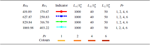


 Open access