


1. Introduction
Fluid dynamics in cylindrical geometries underpins a broad spectrum of engineering and scientific applications. In configurations where the fluid is confined between two concentric cylinders, the flow may develop either in the axial or azimuthal direction. In the former case, referred to as the concentric annular flow, the wall curvature is transverse to the main flow (Quadrio & Luchini Reference Quadrio and Luchini2002); in the latter, known as a curved channel, the curvature is longitudinal. Understanding the contrasting effects of curvature on axial versus azimuthal flows is essential for optimising designs across a range of industries, including oil and gas, and biomedical engineering. In a recent study, Orlandi, Soldati & Pirozzoli (Reference Orlandi, Soldati and Pirozzoli2025) performed direct numerical simulation (DNS) of both configurations at very small and very large values of the inner radius $r_i$
, using the gap width
$r_i$
, using the gap width $\delta = r_o - r_i$
(where
$\delta = r_o - r_i$
(where $r_o$
is the outer radius) as the reference length. For the axial configuration at large
$r_o$
is the outer radius) as the reference length. For the axial configuration at large $r_i$
, the flow exhibits characteristics similar to those of a classical planar channel, with comparable mean wall friction on both boundaries. Conversely, for
$r_i$
, the flow exhibits characteristics similar to those of a classical planar channel, with comparable mean wall friction on both boundaries. Conversely, for $r_i \lt 1$
, the inner-wall friction coefficient (
$r_i \lt 1$
, the inner-wall friction coefficient ( $C_{\kern-1pt f,i}$
) exceeds the outer-wall counterpart (
$C_{\kern-1pt f,i}$
) exceeds the outer-wall counterpart ( $C_{\kern-1pt f,o}$
).
$C_{\kern-1pt f,o}$
).
A notable feature of flow in curved channels is the occurrence of negative turbulent kinetic energy (TKE) production, which Eskinazi & Erian (Reference Eskinazi and Erian1969) attributed to a local ‘energy reversal’ mechanism, wherein energy is transferred from the turbulent fluctuations back to the mean flow. This reversal is associated with the presence of large-scale coherent structures near the convex wall of the curved channel (Soldati, Orlandi & Pirozzoli Reference Soldati, Orlandi and Pirozzoli2025). In this configuration, Orlandi et al. (Reference Orlandi, Soldati and Pirozzoli2025) observed a distinctive behaviour of the friction coefficients $C_{\kern-1pt f,i}$
and
$C_{\kern-1pt f,i}$
and $C_{\kern-1pt f,o}$
as functions of the inner radius
$C_{\kern-1pt f,o}$
as functions of the inner radius $r_i$
, indicating the development of a highly complex flow. This complexity manifests as a region of negative TKE production near the inner wall, along with a pronounced enhancement in the contribution of the pressure–velocity correlation term in the TKE budget, which balances the total dissipation. Such peculiar behaviour in the TKE budget is observed only under conditions of extreme curvature, specifically for
$r_i$
, indicating the development of a highly complex flow. This complexity manifests as a region of negative TKE production near the inner wall, along with a pronounced enhancement in the contribution of the pressure–velocity correlation term in the TKE budget, which balances the total dissipation. Such peculiar behaviour in the TKE budget is observed only under conditions of extreme curvature, specifically for $r_i \lt 0.5$
. These simulations are primarily of academic interest, as replicating such conditions in practical experiments would be highly challenging.
$r_i \lt 0.5$
. These simulations are primarily of academic interest, as replicating such conditions in practical experiments would be highly challenging.
The Taylor–Couette (TC) flow is a more suitable candidate to study curvature effects through laboratory investigation. The flow develops as the result of the relative rotation of two infinitely long, concentric cylinders. Limiting to the case of stationary outer cylinder, which is traditionally the most studied, the flow is controlled by one geometric parameter, for instance the inner-to-outer radius ratio $\eta = r_i / r_o$
, and a Reynolds number, for instance
$\eta = r_i / r_o$
, and a Reynolds number, for instance $ \textit{Re} = V_i \delta /\nu$
, where
$ \textit{Re} = V_i \delta /\nu$
, where $V_i = \omega _i r_i$
and
$V_i = \omega _i r_i$
and $\omega _i$
is the angular velocity of the inner cylinder. TC flow has been extensively studied, both experimentally and numerically, with particular attention to the formation of complex azimuthal structures as the Reynolds number increases. Although it is impossible to mention all of the foundational works, key early contributions certainly include those of Taylor (Reference Taylor1923) and Coles (Reference Coles1965), who visualised wave-like patterns on Taylor vortices that evolve into turbulent structures superimposed on coherent azimuthal modes. A comprehensive review of the literature up to that time was provided by Di Prima & Swinney (Reference Di Prima and Swinney1981), which highlighted that the majority of studies address radius ratios
$\omega _i$
is the angular velocity of the inner cylinder. TC flow has been extensively studied, both experimentally and numerically, with particular attention to the formation of complex azimuthal structures as the Reynolds number increases. Although it is impossible to mention all of the foundational works, key early contributions certainly include those of Taylor (Reference Taylor1923) and Coles (Reference Coles1965), who visualised wave-like patterns on Taylor vortices that evolve into turbulent structures superimposed on coherent azimuthal modes. A comprehensive review of the literature up to that time was provided by Di Prima & Swinney (Reference Di Prima and Swinney1981), which highlighted that the majority of studies address radius ratios $\eta \gt 0.5$
. An important parameter in practical (either experimental and numerical) realisations of TC flow is the aspect ratio
$\eta \gt 0.5$
. An important parameter in practical (either experimental and numerical) realisations of TC flow is the aspect ratio $\varGamma = L/\delta$
, where
$\varGamma = L/\delta$
, where $L$
is the (necessarily finite) axial length of the cylinders. In numerical simulations with
$L$
is the (necessarily finite) axial length of the cylinders. In numerical simulations with $\eta = 0.909$
, Ostilla-Mónico et al. (Reference Ostilla-Mónico, Verzicco and Lohse2015) demonstrated that the torque and mean azimuthal velocity profiles are well captured with
$\eta = 0.909$
, Ostilla-Mónico et al. (Reference Ostilla-Mónico, Verzicco and Lohse2015) demonstrated that the torque and mean azimuthal velocity profiles are well captured with $\varGamma = 2$
. Brauckmann & Eckhardt (Reference Brauckmann and Eckhardt2013a
) employed
$\varGamma = 2$
. Brauckmann & Eckhardt (Reference Brauckmann and Eckhardt2013a
) employed $\varGamma = 2$
and
$\varGamma = 2$
and $\eta = 0.71$
in numerical simulations of TC flow at Reynolds numbers up to
$\eta = 0.71$
in numerical simulations of TC flow at Reynolds numbers up to $30\,000$
, and observed a good collapse of the torque across several experimental and numerical datasets when plotted against the shear Reynolds number,
$30\,000$
, and observed a good collapse of the torque across several experimental and numerical datasets when plotted against the shear Reynolds number, $ \textit{Re}_S = 2 \textit{Re} / (1+\eta )$
, especially for
$ \textit{Re}_S = 2 \textit{Re} / (1+\eta )$
, especially for $\eta \approx 0.7$
.
$\eta \approx 0.7$
.
In general, TC flows in the limit of very small inner radii have received considerably less attention than the more conventional cases with $\eta = O(1)$
, with only a few notable exceptions that will be discussed later. Nevertheless, this regime is of practical relevance. Devices based on TC flow with small rotating inner cylinders can provide efficient mixing at low Reynolds numbers in small volumes of biological fluids, for instance in DNA amplification (Li et al. Reference Li, Li, Yang, Long, Xu, Liu and Zong2024). Further applications arise in the food and cosmetics industries, where controlled mixing of small batches can significantly reduce costs during the research and development phase (Nemri, Charton & Climent Reference Nemri, Charton and Climent2016). In such contexts, achieving a nearly constant shear stress in the gap between the cylinders is desirable, yet difficult to realise in TC flows with order-one radius ratios.
$\eta = O(1)$
, with only a few notable exceptions that will be discussed later. Nevertheless, this regime is of practical relevance. Devices based on TC flow with small rotating inner cylinders can provide efficient mixing at low Reynolds numbers in small volumes of biological fluids, for instance in DNA amplification (Li et al. Reference Li, Li, Yang, Long, Xu, Liu and Zong2024). Further applications arise in the food and cosmetics industries, where controlled mixing of small batches can significantly reduce costs during the research and development phase (Nemri, Charton & Climent Reference Nemri, Charton and Climent2016). In such contexts, achieving a nearly constant shear stress in the gap between the cylinders is desirable, yet difficult to realise in TC flows with order-one radius ratios.
In this paper, we present simulations of TC flow with a stationary outer cylinder, spanning the laminar, transitional and fully turbulent regimes, with a particular emphasis on configurations with very small inner radii, which are systematically compared with the reference cases with $\eta = O(1)$
. One of our primary goals is to assess the most suitable definition of the Taylor number for collapsing the dimensionless torque across a wide range of
$\eta = O(1)$
. One of our primary goals is to assess the most suitable definition of the Taylor number for collapsing the dimensionless torque across a wide range of $\eta$
, including very small values that, to the best of our knowledge, have not been previously explored either numerically or experimentally. In addition, we investigate whether the friction velocity near the inner wall can serve as a basis for scaling the mean flow and turbulence statistics. It is important to note that in the present set-up, the effects of rotation and shear are inherently intertwined, unlike in previous studies. Therefore, comparison with previous studies in which the inner and outer cylinder were independently actuated should be taken with care (Grossmann, Lohse & Sun Reference Grossmann, Lohse and Sun2016).
$\eta$
, including very small values that, to the best of our knowledge, have not been previously explored either numerically or experimentally. In addition, we investigate whether the friction velocity near the inner wall can serve as a basis for scaling the mean flow and turbulence statistics. It is important to note that in the present set-up, the effects of rotation and shear are inherently intertwined, unlike in previous studies. Therefore, comparison with previous studies in which the inner and outer cylinder were independently actuated should be taken with care (Grossmann, Lohse & Sun Reference Grossmann, Lohse and Sun2016).
2. Methodology
The incompressible Navier–Stokes equations in cylindrical coordinates are solved using the second-order finite-difference scheme developed by Verzicco & Orlandi (Reference Verzicco and Orlandi1996). This scheme employs $q_r = r v_r$
as a computational variable, which simplifies the treatment of the axis within the computational domain. Although not strictly necessary for the present configuration, this approach is retained for consistency with the numerical code used for DNS of pipe flow by Orlandi & Fatica (Reference Orlandi and Fatica1997). Time integration of the governing equations is performed using a hybrid third-order low-storage Runge–Kutta algorithm, in which the diffusive terms are treated implicitly and the convective terms are advanced explicitly. The code has been optimised for execution on GPU clusters through a combination of CUDA Fortran and OpenACC directives, and makes use of CUFFT libraries for fast Fourier transforms (FFTs).
$q_r = r v_r$
as a computational variable, which simplifies the treatment of the axis within the computational domain. Although not strictly necessary for the present configuration, this approach is retained for consistency with the numerical code used for DNS of pipe flow by Orlandi & Fatica (Reference Orlandi and Fatica1997). Time integration of the governing equations is performed using a hybrid third-order low-storage Runge–Kutta algorithm, in which the diffusive terms are treated implicitly and the convective terms are advanced explicitly. The code has been optimised for execution on GPU clusters through a combination of CUDA Fortran and OpenACC directives, and makes use of CUFFT libraries for fast Fourier transforms (FFTs).
Unlike some previous studies, since our focus is on flows with $\eta \lt 0.5$
, all simulations are carried out over the full azimuthal extent. An extensive set of runs has been performed covering
$\eta \lt 0.5$
, all simulations are carried out over the full azimuthal extent. An extensive set of runs has been performed covering $0.024 \leqslant \eta \leqslant 0.6$
and
$0.024 \leqslant \eta \leqslant 0.6$
and $80 \leqslant \textit{Re} \leqslant 5000$
. At larger
$80 \leqslant \textit{Re} \leqslant 5000$
. At larger $r_i$
, the configuration of Ostilla-Mónico et al. (Reference Ostilla-Mónico, Van Der, Erwin, Verzicco, Grossmann and Lohse2014) with
$r_i$
, the configuration of Ostilla-Mónico et al. (Reference Ostilla-Mónico, Van Der, Erwin, Verzicco, Grossmann and Lohse2014) with $\eta = 0.714$
has been simulated at intermediate and relatively low Reynolds numbers to validate the present numerical method. The list of high-Reynolds-number simulations is reported in table 1, showing that the computations were carried out over long time intervals – particularly for the smallest
$\eta = 0.714$
has been simulated at intermediate and relatively low Reynolds numbers to validate the present numerical method. The list of high-Reynolds-number simulations is reported in table 1, showing that the computations were carried out over long time intervals – particularly for the smallest $\eta$
– and that the resolution in wall and Kolmogorov units is comparable to that typically employed in canonical wall-bounded flows (Pirozzoli et al. Reference Pirozzoli, Romero, Fatica, Verzicco and Orlandi2021).
$\eta$
– and that the resolution in wall and Kolmogorov units is comparable to that typically employed in canonical wall-bounded flows (Pirozzoli et al. Reference Pirozzoli, Romero, Fatica, Verzicco and Orlandi2021).
Flow parameters: inner radius ( $r_i$
), corresponding inner-to-outer radius ratio (
$r_i$
), corresponding inner-to-outer radius ratio ( $\eta$
); simulation time in code units (
$\eta$
); simulation time in code units ( $T_F$
), in wall units (
$T_F$
), in wall units ( $T_F^+$
) and in Kolmogorov units (
$T_F^+$
) and in Kolmogorov units ( $T_F^*$
); grid resolution in wall units and in Kolmogorov units (in parentheses), with Kolmogorov scale evaluated at the peak position of
$T_F^*$
); grid resolution in wall units and in Kolmogorov units (in parentheses), with Kolmogorov scale evaluated at the peak position of $K$
(
$K$
( $r_K$
).
$r_K$
).

3. Results
3.1. Torque
Before presenting the full set of simulated cases, it is useful to discuss possible definitions of the Taylor number and to examine whether any of them provides a consistent parametrisation of the torque for arbitrary $\eta$
in the case of a stationary outer cylinder. For example, Di Prima & Swinney (Reference Di Prima and Swinney1981) define the Taylor number as
$\eta$
in the case of a stationary outer cylinder. For example, Di Prima & Swinney (Reference Di Prima and Swinney1981) define the Taylor number as $ \textit{Ta}_d = 4 \, (1 - \eta ) / (1 + \eta ) \, \textit{Re}^2$
, whereas Ostilla-Mónico et al. (Reference Ostilla-Mónico, Verzicco and Lohse2015) use
$ \textit{Ta}_d = 4 \, (1 - \eta ) / (1 + \eta ) \, \textit{Re}^2$
, whereas Ostilla-Mónico et al. (Reference Ostilla-Mónico, Verzicco and Lohse2015) use $ \textit{Ta}_o = \sigma (1 / \eta + 1) \textit{Re}^2$
, with the geometric factor
$ \textit{Ta}_o = \sigma (1 / \eta + 1) \textit{Re}^2$
, with the geometric factor $\sigma = (1 + \eta )^4 / (4 \eta )^2$
. Brauckmann & Eckhardt (Reference Brauckmann and Eckhardt2013a
) further propose
$\sigma = (1 + \eta )^4 / (4 \eta )^2$
. Brauckmann & Eckhardt (Reference Brauckmann and Eckhardt2013a
) further propose $ \textit{Ta}_b = \sigma ^2 \textit{Re}_S^2$
. According to all these definitions, the Taylor number typically increases with
$ \textit{Ta}_b = \sigma ^2 \textit{Re}_S^2$
. According to all these definitions, the Taylor number typically increases with $\eta$
up to
$\eta$
up to $\eta = 0.5$
, and then either decreases or approaches a plateau for
$\eta = 0.5$
, and then either decreases or approaches a plateau for $\eta \gt 0.5$
. In contrast, Chandrasekhar (Reference Chandrasekhar1961, p. 296, (169)) define the Taylor number (for a stationary outer cylinder) as
$\eta \gt 0.5$
. In contrast, Chandrasekhar (Reference Chandrasekhar1961, p. 296, (169)) define the Taylor number (for a stationary outer cylinder) as $ \textit{Ta}_c = 4 \textit{Re}^2 \eta ^2 / (1 - \eta )^4 / (1 + \eta )^2$
, which yields a quadratic dependence for small
$ \textit{Ta}_c = 4 \textit{Re}^2 \eta ^2 / (1 - \eta )^4 / (1 + \eta )^2$
, which yields a quadratic dependence for small $\eta$
and steeper growth as
$\eta$
and steeper growth as $\eta \to 1$
.
$\eta \to 1$
.
The key output in TC flow is the non-dimensional torque, defined as
 \begin{align} \textit{Nu}^\omega = \frac {J^\omega }{J^\omega _0} = \frac {r^3 \left ( \langle v_r' v_\theta ' \rangle - \dfrac {1}{\textit{Re}} \dfrac {\partial (\langle v_\theta \rangle / r)}{\partial r} \right )}{J^\omega _0} = \textit{Nu}_T + \textit{Nu}_V, \hskip 1.em J^\omega _0 = \frac {1}{\textit{Re}} \frac {2 r_i r_o^2}{r_i + r_o}, \end{align}
where $ \textit{Nu}_T$
and
$ \textit{Nu}_T$
and $ \textit{Nu}_V$
are the turbulent and viscous contributions, respectively, and
$ \textit{Nu}_V$
are the turbulent and viscous contributions, respectively, and $J^\omega _0$
denotes the value in laminar flow. In (3.1), the angle brackets
$J^\omega _0$
denotes the value in laminar flow. In (3.1), the angle brackets $\langle \, \rangle$
denote averaging in time and over the azimuthal (
$\langle \, \rangle$
denote averaging in time and over the azimuthal ( $\theta$
) and axial (
$\theta$
) and axial ( $z$
) directions. Momentum conservation implies that
$z$
) directions. Momentum conservation implies that $ \textit{Nu}^\omega$
must remain exactly constant across the radial direction; therefore, the statistical convergence of the numerical simulations can be assessed from deviations from this constancy. This requirement is particularly stringent for flows with very small
$ \textit{Nu}^\omega$
must remain exactly constant across the radial direction; therefore, the statistical convergence of the numerical simulations can be assessed from deviations from this constancy. This requirement is particularly stringent for flows with very small $\eta$
, since a long integration time is needed for the inner cylinder to transfer angular momentum to the entire flow field. This constraint helps explain why such configurations have seldom been explored in previous simulations or experiments. Moreover, it has been found that the grid resolution can significantly influence the accuracy of the computed torque, especially in cases with extremely small inner radii.
$\eta$
, since a long integration time is needed for the inner cylinder to transfer angular momentum to the entire flow field. This constraint helps explain why such configurations have seldom been explored in previous simulations or experiments. Moreover, it has been found that the grid resolution can significantly influence the accuracy of the computed torque, especially in cases with extremely small inner radii.
Eckhardt, Grossmann & Lohse (Reference Eckhardt, Grossmann and Lohse2007) provided a detailed derivation of the non-dimensional torque expression starting from the Navier–Stokes equations, concluding that the proper field to consider as the transported quantity is the angular velocity, $\omega = v_\theta / r$
, rather than the azimuthal velocity or the angular momentum,
$\omega = v_\theta / r$
, rather than the azimuthal velocity or the angular momentum, $L = r v_\theta$
. From a numerical standpoint, it is important to note that radial derivatives appear in the expression for
$L = r v_\theta$
. From a numerical standpoint, it is important to note that radial derivatives appear in the expression for $ \textit{Nu}^\omega$
. Their evaluation on strongly non-uniform grids – required to achieve higher resolution near the walls – may depend on the variable locations and the quantity being differentiated. For instance, we have found that more accurate results near the walls are obtained by expressing
$ \textit{Nu}^\omega$
. Their evaluation on strongly non-uniform grids – required to achieve higher resolution near the walls – may depend on the variable locations and the quantity being differentiated. For instance, we have found that more accurate results near the walls are obtained by expressing
 \begin{align} {\partial \langle \omega \rangle }/{\partial r} = {\partial \langle v_\theta \rangle / r}/{\partial r} = \left ( \langle \omega _z \rangle - 2 {\langle v_\theta \rangle }/{r} \right ) / r . \end{align}
It is important to recall that in the staggered numerical discretisation that we are using, the velocity components are defined at the centres of the cell faces; hence, the vorticity components are located at the centres of the edges (e.g. $\omega _z(i,j,k+1/2)$
). Therefore, derivatives as
$\omega _z(i,j,k+1/2)$
). Therefore, derivatives as ${\partial \langle \omega \rangle }/{\partial r}$
are evaluated at the grid index
${\partial \langle \omega \rangle }/{\partial r}$
are evaluated at the grid index $j$
.
$j$
.
For the more general case in which the outer cylinder also rotates independently, Brauckmann & Eckhardt (Reference Brauckmann and Eckhardt2013 b) decomposed the numerator of (3.1), into a large-scale component – representing the mean variations in the radial and axial directions – and the turbulent fluctuations. The evaluation of this decomposition is rather involved, as it requires axially shifting the instantaneous flow field to keep the Taylor vortices at a fixed height. The results reported by Brauckmann & Eckhardt (Reference Brauckmann and Eckhardt2013b , figure 4,,) show that, for the special case of a stationary outer cylinder as the present one, the two contributions are nearly identical.
To highlight the pronounced differences in the flow near the inner and outer cylinders, Eckhardt et al. (Reference Eckhardt, Grossmann and Lohse2007) noted that, at steady state,
 \begin{align} \left . \frac {\partial \langle \omega \rangle }{\partial r} \right |_o = \eta ^3 \left . \frac {\partial \langle \omega \rangle }{\partial r} \right |_i. \end{align}
The time evolution of the two sides of this relation illustrates the approach to steady state and demonstrates that, for small $\eta$
, the simulations must be run for long durations before
$\eta$
, the simulations must be run for long durations before $\eta ^3 \left . {\partial \langle \omega \rangle }/{\partial r} \right |_i$
converges to
$\eta ^3 \left . {\partial \langle \omega \rangle }/{\partial r} \right |_i$
converges to $\left . {\partial \langle \omega \rangle }/{\partial r} \right |_o$
. The relevant values are reported in table 2. It is worth noting that, for very small
$\left . {\partial \langle \omega \rangle }/{\partial r} \right |_o$
. The relevant values are reported in table 2. It is worth noting that, for very small $\eta$
, the wall-normal gradients at the two boundaries differ significantly, with the difference decreasing rapidly as
$\eta$
, the wall-normal gradients at the two boundaries differ significantly, with the difference decreasing rapidly as $\eta$
increases. The identity (3.3) is indeed satisfied with good accuracy. Figure 1(a) further illustrates that, for small
$\eta$
increases. The identity (3.3) is indeed satisfied with good accuracy. Figure 1(a) further illustrates that, for small $\eta$
, (3.3) is satisfied with fewer samples than for larger
$\eta$
, (3.3) is satisfied with fewer samples than for larger $\eta$
(see figure 1
b). Table 2 corresponds to
$\eta$
(see figure 1
b). Table 2 corresponds to $ \textit{Re} = 5000$
, at which a fully turbulent regime is established.
$ \textit{Re} = 5000$
, at which a fully turbulent regime is established.
Time evolution (in the last thousand time units) of the terms in the identity (3.3), namely ${\partial \omega }/{\partial r}|_o$
(solid symbols) and
${\partial \omega }/{\partial r}|_o$
(solid symbols) and $-\eta ^3 {\partial \omega }/{\partial r}|_i$
(open symbols). Data at
$-\eta ^3 {\partial \omega }/{\partial r}|_i$
(open symbols). Data at $\eta \lt 0.2$
are shown in panel (a) and data at
$\eta \lt 0.2$
are shown in panel (a) and data at $\eta \geqslant 0.2$
are shown in panel (b). For all cases
$\eta \geqslant 0.2$
are shown in panel (b). For all cases $ \textit{Re}=5000$
, with values of
$ \textit{Re}=5000$
, with values of $\eta$
provided in table 1.
$\eta$
provided in table 1.

A further verification can be made by evaluating the resolution as a fraction of the Kolmogorov scale, whose local value we estimate as
 \begin{align} \ell _{\eta } = \big(\nu ^3/\mathcal{D} \big)^{1/4}, \end{align}
where $\mathcal{D}$
is the total dissipation, which will be defined later. The grid spacing in Kolmogorov units is provided in table 1 (the values in parentheses), where
$\mathcal{D}$
is the total dissipation, which will be defined later. The grid spacing in Kolmogorov units is provided in table 1 (the values in parentheses), where $\ell _{\eta }$
is evaluated for each flow case at the peak location of the turbulent kinetic energy. Again, the table confirms that the simulations are properly resolved.
$\ell _{\eta }$
is evaluated for each flow case at the peak location of the turbulent kinetic energy. Again, the table confirms that the simulations are properly resolved.
Flow parameters: $\eta$
, maximum and minimum per cent errors of
$\eta$
, maximum and minimum per cent errors of $1-Nu^\omega /\langle Nu^\omega \rangle$
, friction Reynolds number
$1-Nu^\omega /\langle Nu^\omega \rangle$
, friction Reynolds number $R_\tau =u_\tau \textit{Re}$
at the inner and outer cylinders, Kolmogorov length scale evaluated with the total dissipation at location of maximum
$R_\tau =u_\tau \textit{Re}$
at the inner and outer cylinders, Kolmogorov length scale evaluated with the total dissipation at location of maximum $K^+$
, derivatives of the angular velocity at the inner and outer cylinders.
$K^+$
, derivatives of the angular velocity at the inner and outer cylinders.

Table 2 also reports minimum and maximum values of $\varepsilon _{\textit{Nu}} = 1 - Nu^\omega /\langle Nu^\omega \rangle$
, which can be interpreted as deviations from perfect time convergence and satisfactory grid resolution. For
$\varepsilon _{\textit{Nu}} = 1 - Nu^\omega /\langle Nu^\omega \rangle$
, which can be interpreted as deviations from perfect time convergence and satisfactory grid resolution. For $\eta = O(1)$
, the errors are similar to those reported by Ostilla-Mónico et al. (Reference Ostilla-Mónico, Stevens, Grossmann, Verzicco and Lohse2013). Slightly higher errors are found at low
$\eta = O(1)$
, the errors are similar to those reported by Ostilla-Mónico et al. (Reference Ostilla-Mónico, Stevens, Grossmann, Verzicco and Lohse2013). Slightly higher errors are found at low $\eta$
, which could be partly due to discretisation errors in the evaluation of the radial derivative of
$\eta$
, which could be partly due to discretisation errors in the evaluation of the radial derivative of $\langle \omega \rangle$
under such conditions. As reported in table 2, the time convergence error strongly depends on
$\langle \omega \rangle$
under such conditions. As reported in table 2, the time convergence error strongly depends on $\eta$
. To identify the regions within the gap which contribute most to the error, in figure 2, we show profiles of
$\eta$
. To identify the regions within the gap which contribute most to the error, in figure 2, we show profiles of $\varepsilon _{\textit{Nu}}$
. It is evident that only in the cases with extremely small
$\varepsilon _{\textit{Nu}}$
. It is evident that only in the cases with extremely small $\eta$
does a peak appear near the inner cylinder, which coincides with the region where
$\eta$
does a peak appear near the inner cylinder, which coincides with the region where $ \textit{Nu}_V$
sharply decreases. As previously mentioned, in this region, the evaluation of radial derivatives on a non-uniform grid is sensitive to the numerical scheme used. This peak decreases as
$ \textit{Nu}_V$
sharply decreases. As previously mentioned, in this region, the evaluation of radial derivatives on a non-uniform grid is sensitive to the numerical scheme used. This peak decreases as $\eta$
increases and the resulting distributions become similar to those reported by Ostilla-Mónico et al. (Reference Ostilla-Mónico, Stevens, Grossmann, Verzicco and Lohse2013), although their results refer to a lower Reynolds number
$\eta$
increases and the resulting distributions become similar to those reported by Ostilla-Mónico et al. (Reference Ostilla-Mónico, Stevens, Grossmann, Verzicco and Lohse2013), although their results refer to a lower Reynolds number $ \textit{Re} = 1600$
compared with the present case with
$ \textit{Re} = 1600$
compared with the present case with $ \textit{Re} = 5000$
.
$ \textit{Re} = 5000$
.
Profiles of local torque unbalance, $\varepsilon _{\textit{Nu}}=1-Nu^\omega /\langle Nu^\omega \rangle$
, obtained by averaging the last thousand profiles saved every one non-dimensional time unit, for values of
$\varepsilon _{\textit{Nu}}=1-Nu^\omega /\langle Nu^\omega \rangle$
, obtained by averaging the last thousand profiles saved every one non-dimensional time unit, for values of $\eta$
indicated in table 1 (
$\eta$
indicated in table 1 ( $ \textit{Re}=5000$
for all cases).
$ \textit{Re}=5000$
for all cases).

As stated in § 1, most previous numerical and experimental studies were conducted for $\eta \gt 0.5$
, for which good collapse of the
$\eta \gt 0.5$
, for which good collapse of the $ \textit{Nu}^\omega {-}\textit{Ta}$
relationship is obtained regardless of the definition of
$ \textit{Nu}^\omega {-}\textit{Ta}$
relationship is obtained regardless of the definition of $ \textit{Ta}$
. As a preliminary step, we have computed two of the test cases carried out by Ostilla-Mónico et al. (Reference Ostilla-Mónico, Verzicco and Lohse2015). The first case correspond to
$ \textit{Ta}$
. As a preliminary step, we have computed two of the test cases carried out by Ostilla-Mónico et al. (Reference Ostilla-Mónico, Verzicco and Lohse2015). The first case correspond to $ \textit{Re}=80$
,
$ \textit{Re}=80$
, $\eta =0.5$
,
$\eta =0.5$
, $\varGamma =2$
, with a
$\varGamma =2$
, with a $32\times 64\times 64$
grid and a rotational symmetry of order four, for which we find
$32\times 64\times 64$
grid and a rotational symmetry of order four, for which we find $ \textit{Nu}^\omega =1.136$
, in good agreement with their value
$ \textit{Nu}^\omega =1.136$
, in good agreement with their value $ \textit{Nu}^\omega =1.138$
. The second case corresponds to
$ \textit{Nu}^\omega =1.138$
. The second case corresponds to $ \textit{Re}=1120$
,
$ \textit{Re}=1120$
, $\eta =5/7$
,
$\eta =5/7$
, $\varGamma =2\pi$
, which as in Ostilla-Mónico et al. (Reference Ostilla-Mónico, Verzicco and Lohse2015), we have computed with an unresolved and a fully resolved mesh, with rotational symmetry of order 4. Ostilla-Mónico et al. (Reference Ostilla-Mónico, Verzicco and Lohse2015) found that, depending on the initial conditions, four or three pairs of Taylor vortices may form, with associated slight differences in
$\varGamma =2\pi$
, which as in Ostilla-Mónico et al. (Reference Ostilla-Mónico, Verzicco and Lohse2015), we have computed with an unresolved and a fully resolved mesh, with rotational symmetry of order 4. Ostilla-Mónico et al. (Reference Ostilla-Mónico, Verzicco and Lohse2015) found that, depending on the initial conditions, four or three pairs of Taylor vortices may form, with associated slight differences in $ \textit{Nu}^\omega$
. In the unresolved simulation, we find
$ \textit{Nu}^\omega$
. In the unresolved simulation, we find $ \textit{Nu}^\omega =4.809$
, as compared with
$ \textit{Nu}^\omega =4.809$
, as compared with $ \textit{Nu}^\omega =4.835$
. In the well-resolved simulation, we find instead
$ \textit{Nu}^\omega =4.835$
. In the well-resolved simulation, we find instead $ \textit{Nu}^\omega =4.688$
, as compared with
$ \textit{Nu}^\omega =4.688$
, as compared with $ \textit{Nu}^\omega =4.478$
, with a
$ \textit{Nu}^\omega =4.478$
, with a $4.7\,\%$
difference. This difference may be due to the way that
$4.7\,\%$
difference. This difference may be due to the way that $ \textit{Nu}^\omega$
is evaluated. For instance, we estimate
$ \textit{Nu}^\omega$
is evaluated. For instance, we estimate $ \textit{Nu}^\omega$
by averaging the total torque along the radial direction.
$ \textit{Nu}^\omega$
by averaging the total torque along the radial direction.
Representative distributions of $ \textit{Nu}^\omega$
are reported in figure 3, as obtained in a domain with
$ \textit{Nu}^\omega$
are reported in figure 3, as obtained in a domain with $\varGamma =2$
, without any assumed rotational symmetry. At low Reynolds number (
$\varGamma =2$
, without any assumed rotational symmetry. At low Reynolds number ( $ \textit{Re}=800$
), figure 3(a) shows that for
$ \textit{Re}=800$
), figure 3(a) shows that for $\eta =0.0244$
,
$\eta =0.0244$
, $ \textit{Nu}_T$
is smaller than
$ \textit{Nu}_T$
is smaller than $ \textit{Nu}_V$
, indicating that the flow is nearly laminar. In contrast, for
$ \textit{Nu}_V$
, indicating that the flow is nearly laminar. In contrast, for $\eta =0.5$
, the flow remains turbulent and
$\eta =0.5$
, the flow remains turbulent and $ \textit{Nu}^\omega$
decreases with decreasing
$ \textit{Nu}^\omega$
decreases with decreasing $ \textit{Re}$
. At
$ \textit{Re}$
. At $ \textit{Re}=1600$
, the simulation performed on a
$ \textit{Re}=1600$
, the simulation performed on a $192 \times 192 \times 128$
grid (figure 3
b) yields a nearly constant
$192 \times 192 \times 128$
grid (figure 3
b) yields a nearly constant $ \textit{Nu}^\omega$
profile. It is also noteworthy that, for
$ \textit{Nu}^\omega$
profile. It is also noteworthy that, for $\eta =0.5$
, the turbulent contribution
$\eta =0.5$
, the turbulent contribution $ \textit{Nu}_T$
decreases with distance from the inner wall near the centre of the gap, with a corresponding increase in the viscous contribution
$ \textit{Nu}_T$
decreases with distance from the inner wall near the centre of the gap, with a corresponding increase in the viscous contribution $ \textit{Nu}_V$
, thereby maintaining a constant total torque. The difference between
$ \textit{Nu}_V$
, thereby maintaining a constant total torque. The difference between $ \textit{Nu}_T$
and
$ \textit{Nu}_T$
and $ \textit{Nu}_V$
diminishes as
$ \textit{Nu}_V$
diminishes as $\eta$
and
$\eta$
and $ \textit{Re}$
decrease. For instance, at
$ \textit{Re}$
decrease. For instance, at $\eta =0.0244$
in figure 3(b), the two contributions are approximately in balance around the gap centre. Figure 3(c) and 3(d) illustrate the influence of grid resolution at higher Reynolds numbers (
$\eta =0.0244$
in figure 3(b), the two contributions are approximately in balance around the gap centre. Figure 3(c) and 3(d) illustrate the influence of grid resolution at higher Reynolds numbers ( $ \textit{Re}=5000$
). When the resolution is insufficient, as shown in figure 3(c), undulations in the profile of
$ \textit{Re}=5000$
). When the resolution is insufficient, as shown in figure 3(c), undulations in the profile of $ \textit{Nu}^\omega$
appear near both walls. These undulations are primarily attributed to variations in the turbulent contribution
$ \textit{Nu}^\omega$
appear near both walls. These undulations are primarily attributed to variations in the turbulent contribution $ \textit{Nu}_T$
, and their amplitude increases with larger values of
$ \textit{Nu}_T$
, and their amplitude increases with larger values of $\eta$
. In contrast, the results from higher- resolution simulations, presented in figure 3(d), show a clear reduction in the amplitude of these undulations and a lower overall value of
$\eta$
. In contrast, the results from higher- resolution simulations, presented in figure 3(d), show a clear reduction in the amplitude of these undulations and a lower overall value of $ \textit{Nu}^\omega$
for
$ \textit{Nu}^\omega$
for $\eta =0.5$
. At
$\eta =0.5$
. At $\eta =0.0244$
, the magnitude of the two contributions to
$\eta =0.0244$
, the magnitude of the two contributions to $ \textit{Nu}^\omega$
, shown in both figure 3(c) and 3(d), does not significantly change with resolution. However, the more refined simulation yields a more uniform
$ \textit{Nu}^\omega$
, shown in both figure 3(c) and 3(d), does not significantly change with resolution. However, the more refined simulation yields a more uniform $ \textit{Nu}^\omega$
profile across the entire gap.
$ \textit{Nu}^\omega$
profile across the entire gap.
Distributions of non-dimensional total torque $ \textit{Nu}^\omega$
(lines), and its turbulent (
$ \textit{Nu}^\omega$
(lines), and its turbulent ( $ \textit{Nu}_T$
, open circles) and viscous (
$ \textit{Nu}_T$
, open circles) and viscous ( $ \textit{Nu}_V$
, solid circles) components, versus distance from the inner wall for
$ \textit{Nu}_V$
, solid circles) components, versus distance from the inner wall for $\eta =0.0244$
(red) and
$\eta =0.0244$
(red) and $\eta =0.5$
(green): (a)
$\eta =0.5$
(green): (a) $ \textit{Re}=800$
for
$ \textit{Re}=800$
for $\eta =0.0244$
(
$\eta =0.0244$
( $192\times 192 \times 128$
grid) and for
$192\times 192 \times 128$
grid) and for $\eta =0.5$
(
$\eta =0.5$
( $384 \times 192 \times 128$
grid); (b)
$384 \times 192 \times 128$
grid); (b) $ \textit{Re}=1600$
for
$ \textit{Re}=1600$
for $\eta =0.0244$
(
$\eta =0.0244$
( $192\times 192 \times 128$
grid) and for
$192\times 192 \times 128$
grid) and for $\eta =0.5$
(
$\eta =0.5$
( $384 \times 192 \times 128$
grid); (c)
$384 \times 192 \times 128$
grid); (c) $ \textit{Re}=5000$
with same resolution as for
$ \textit{Re}=5000$
with same resolution as for $ \textit{Re}=1600$
; (d)
$ \textit{Re}=1600$
; (d) $ \textit{Re}=5000$
for
$ \textit{Re}=5000$
for $\eta =0.0244$
(
$\eta =0.0244$
( $256\times 256 \times 256$
grid) and for
$256\times 256 \times 256$
grid) and for $\eta =0.5$
(
$\eta =0.5$
( $384 \times 384 \times 256$
grid).
$384 \times 384 \times 256$
grid).

Total torque coefficient ( $ \textit{Nu}^\omega$
) as a function of: (a)
$ \textit{Nu}^\omega$
) as a function of: (a) $ \textit{Re}_S$
; (b)
$ \textit{Re}_S$
; (b) $ \textit{Ta}_o$
; (c)
$ \textit{Ta}_o$
; (c) $ \textit{Ta}_c$
and (d) compensated
$ \textit{Ta}_c$
and (d) compensated $ \textit{Nu}^\omega / \textit{Ta}_c^{1/3}$
versus
$ \textit{Nu}^\omega / \textit{Ta}_c^{1/3}$
versus $ \textit{Ta}_c$
. In panel (a), the inset shows reference data from the literature: Brauckmann & Eckhardt (Reference Brauckmann and Eckhardt2013a
), Wendt (Reference Wendt1933), Froitzheim et al. (Reference Froitzheim, Merbold, Ostilla-Mónico and Egbers2019), Hamede, Merbold & Egbers (Reference Hamede, Merbold and Egbers2023), Ostilla-Mónico et al. (Reference Ostilla-Mónico, Stevens, Grossmann, Verzicco and Lohse2013, table 1), Ostilla-Mónico et al. (Reference Ostilla-Mónico, Van Der, Erwin, Verzicco, Grossmann and Lohse2014, table 1), Lewis & Swinney (Reference Lewis and Swinney1999) and Racina & Kind (Reference Racina and Kind2006). A large part of these data has been extracted by Brauckmann & Eckhardt (Reference Brauckmann and Eckhardt2013a
, figure 11a). The values of
$ \textit{Ta}_c$
. In panel (a), the inset shows reference data from the literature: Brauckmann & Eckhardt (Reference Brauckmann and Eckhardt2013a
), Wendt (Reference Wendt1933), Froitzheim et al. (Reference Froitzheim, Merbold, Ostilla-Mónico and Egbers2019), Hamede, Merbold & Egbers (Reference Hamede, Merbold and Egbers2023), Ostilla-Mónico et al. (Reference Ostilla-Mónico, Stevens, Grossmann, Verzicco and Lohse2013, table 1), Ostilla-Mónico et al. (Reference Ostilla-Mónico, Van Der, Erwin, Verzicco, Grossmann and Lohse2014, table 1), Lewis & Swinney (Reference Lewis and Swinney1999) and Racina & Kind (Reference Racina and Kind2006). A large part of these data has been extracted by Brauckmann & Eckhardt (Reference Brauckmann and Eckhardt2013a
, figure 11a). The values of $\eta$
corresponding to the present simulations are listed in table 1. Solid triangles denote our results for four cases with the same geometry of Ostilla-Mónico et al. (Reference Ostilla-Mónico, Van Der, Erwin, Verzicco, Grossmann and Lohse2014). In panel (a), the green and red lines indicate the trends
$\eta$
corresponding to the present simulations are listed in table 1. Solid triangles denote our results for four cases with the same geometry of Ostilla-Mónico et al. (Reference Ostilla-Mónico, Van Der, Erwin, Verzicco, Grossmann and Lohse2014). In panel (a), the green and red lines indicate the trends $ \textit{Re}_S^{0.4}$
, while the black line represents
$ \textit{Re}_S^{0.4}$
, while the black line represents $ \textit{Re}_S^{0.67}$
. In panel (c), the black lines indicate the trend
$ \textit{Re}_S^{0.67}$
. In panel (c), the black lines indicate the trend $ \textit{Ta}^{2/9}$
and the short blue line is
$ \textit{Ta}^{2/9}$
and the short blue line is $27 \textit{Ta}^{1/3}$
.
$27 \textit{Ta}^{1/3}$
.

In figure 4, we consider possible parametrisations of the torque coefficient, using fully resolved simulations with $\varGamma =2$
and without any rotational symmetry for flows with
$\varGamma =2$
and without any rotational symmetry for flows with $\eta \leqslant 0.5$
at low and high values of Reynolds numbers. Brauckmann & Eckhardt (Reference Brauckmann and Eckhardt2013a
) conducted numerical simulations of TC flow and compiled both numerical and experimental data, showing in their figure 11(a) a satisfactory collapse of
$\eta \leqslant 0.5$
at low and high values of Reynolds numbers. Brauckmann & Eckhardt (Reference Brauckmann and Eckhardt2013a
) conducted numerical simulations of TC flow and compiled both numerical and experimental data, showing in their figure 11(a) a satisfactory collapse of $ \textit{Nu}^\omega$
as a function of the shear Reynolds number
$ \textit{Nu}^\omega$
as a function of the shear Reynolds number $ \textit{Re}_S$
. It is important to note that their dataset corresponds to
$ \textit{Re}_S$
. It is important to note that their dataset corresponds to $\eta \approx 0.7$
. For these cases, at relatively low Reynolds numbers, they reported a scaling law of the form
$\eta \approx 0.7$
. For these cases, at relatively low Reynolds numbers, they reported a scaling law of the form $ \textit{Nu}^\omega = \textit{Re}_S^{0.67}$
. They further noted that this exponent is close to the value
$ \textit{Nu}^\omega = \textit{Re}_S^{0.67}$
. They further noted that this exponent is close to the value $0.69$
obtained by Lewis & Swinney (Reference Lewis and Swinney1999) in experiments conducted at much higher Reynolds numbers and discussed other values of the exponent reported in the literature.
$0.69$
obtained by Lewis & Swinney (Reference Lewis and Swinney1999) in experiments conducted at much higher Reynolds numbers and discussed other values of the exponent reported in the literature.
Several previous studies have examined TC flow at different values of $\eta$
. For instance, Hamede et al. (Reference Hamede, Merbold and Egbers2023) carried out experiments at the relatively small
$\eta$
. For instance, Hamede et al. (Reference Hamede, Merbold and Egbers2023) carried out experiments at the relatively small $\eta = 0.1$
, close to the present configuration, and their results as a function of
$\eta = 0.1$
, close to the present configuration, and their results as a function of $ \textit{Re}_S$
are shown in figure 4(a). These results at high Reynolds number do not align with our simulations at
$ \textit{Re}_S$
are shown in figure 4(a). These results at high Reynolds number do not align with our simulations at $\eta =0.1$
and low
$\eta =0.1$
and low $ \textit{Re}$
(green solid circles in figure 4
a). Numerical results at
$ \textit{Re}$
(green solid circles in figure 4
a). Numerical results at $\eta = 0.317$
, experimental data from figure 2 of Froitzheim et al. (Reference Froitzheim, Merbold, Ostilla-Mónico and Egbers2019) and the classic measurements of Wendt (Reference Wendt1933) at very high Reynolds numbers for
$\eta = 0.317$
, experimental data from figure 2 of Froitzheim et al. (Reference Froitzheim, Merbold, Ostilla-Mónico and Egbers2019) and the classic measurements of Wendt (Reference Wendt1933) at very high Reynolds numbers for $\eta \gt 0.68$
are also reported in figure 4(a). These comparisons indicate that the present simulations, covering both low and high Reynolds numbers, provide an opportunity to assess whether a transitional value of
$\eta \gt 0.68$
are also reported in figure 4(a). These comparisons indicate that the present simulations, covering both low and high Reynolds numbers, provide an opportunity to assess whether a transitional value of $ \textit{Re}_S$
can be identified and correlated with
$ \textit{Re}_S$
can be identified and correlated with $\eta$
. As shown in figure 4(a), for
$\eta$
. As shown in figure 4(a), for $\eta = 0.5$
(slightly smaller than the value considered by Brauckmann & Eckhardt (Reference Brauckmann and Eckhardt2013a
)), simulations with
$\eta = 0.5$
(slightly smaller than the value considered by Brauckmann & Eckhardt (Reference Brauckmann and Eckhardt2013a
)), simulations with $\varGamma = 2$
at high
$\varGamma = 2$
at high $ \textit{Re}$
yield the scaling
$ \textit{Re}$
yield the scaling $ \textit{Nu}^\omega \approx \textit{Re}_S^{0.67}$
. This trend is also consistent with the data of Froitzheim et al. (Reference Froitzheim, Merbold, Ostilla-Mónico and Egbers2019) and, despite some scatter, with the low-
$ \textit{Nu}^\omega \approx \textit{Re}_S^{0.67}$
. This trend is also consistent with the data of Froitzheim et al. (Reference Froitzheim, Merbold, Ostilla-Mónico and Egbers2019) and, despite some scatter, with the low- $ \textit{Re}$
experiments of Hamede et al. (Reference Hamede, Merbold and Egbers2023). Notably, our results for
$ \textit{Re}$
experiments of Hamede et al. (Reference Hamede, Merbold and Egbers2023). Notably, our results for $\eta = 0.5$
align with the classical scaling law
$\eta = 0.5$
align with the classical scaling law $ \textit{Nu}^\omega = \textit{Re}_S^{0.67}$
, which at high
$ \textit{Nu}^\omega = \textit{Re}_S^{0.67}$
, which at high $ \textit{Re}_S$
is supported by the experimental measurements of Wendt (Reference Wendt1933) and Lewis & Swinney (Reference Lewis and Swinney1999), as well as by the high-
$ \textit{Re}_S$
is supported by the experimental measurements of Wendt (Reference Wendt1933) and Lewis & Swinney (Reference Lewis and Swinney1999), as well as by the high- $ \textit{Re}$
simulations of Brauckmann & Eckhardt (Reference Brauckmann and Eckhardt2013a
). The results of Ostilla-Mónico et al. (Reference Ostilla-Mónico, Van Der, Erwin, Verzicco, Grossmann and Lohse2014) at large Reynolds numbers also agree well with those of Wendt (Reference Wendt1933), and up to
$ \textit{Re}$
simulations of Brauckmann & Eckhardt (Reference Brauckmann and Eckhardt2013a
). The results of Ostilla-Mónico et al. (Reference Ostilla-Mónico, Van Der, Erwin, Verzicco, Grossmann and Lohse2014) at large Reynolds numbers also agree well with those of Wendt (Reference Wendt1933), and up to $ \textit{Re}_S = 10^5$
, they coincide with the measurements of Lewis & Swinney (Reference Lewis and Swinney1999). In the same figure, our simulation at
$ \textit{Re}_S = 10^5$
, they coincide with the measurements of Lewis & Swinney (Reference Lewis and Swinney1999). In the same figure, our simulation at $\eta = 0.714$
and
$\eta = 0.714$
and $ \textit{Re} = 37\,400$
falls within the range where the scaling
$ \textit{Re} = 37\,400$
falls within the range where the scaling $ \textit{Nu}^\omega \approx \textit{Re}_S^{0.67}$
holds. In this regime, the relation
$ \textit{Nu}^\omega \approx \textit{Re}_S^{0.67}$
holds. In this regime, the relation $ \textit{Nu}^\omega \approx \textit{Ta}^{1/3}$
emerges and at higher values, a gradual tendency towards the ultimate regime becomes apparent, as discussed later. At lower Reynolds numbers (
$ \textit{Nu}^\omega \approx \textit{Ta}^{1/3}$
emerges and at higher values, a gradual tendency towards the ultimate regime becomes apparent, as discussed later. At lower Reynolds numbers ( $ \textit{Re} \lt 5000$
), the scaling becomes
$ \textit{Re} \lt 5000$
), the scaling becomes $ \textit{Nu}^\omega \approx \textit{Re}_S^{0.40}$
. These latter results, obtained for
$ \textit{Nu}^\omega \approx \textit{Re}_S^{0.40}$
. These latter results, obtained for $800 \lt \textit{Re} \lt 2400$
, correspond to flows where
$800 \lt \textit{Re} \lt 2400$
, correspond to flows where $ \textit{Nu}_T \leqslant Nu_V$
in the central gap region, although both contributions remain non-uniform. In contrast, in cases where
$ \textit{Nu}_T \leqslant Nu_V$
in the central gap region, although both contributions remain non-uniform. In contrast, in cases where $ \textit{Nu}^\omega \approx \textit{Re}_S^{0.67}$
, both the turbulent and viscous contributions are approximately constant across the central region, indicating fully developed turbulence unaffected by the coherent structures that typically form near the inner cylinder. This aspect will be revisited later with the aid of flow visualisations. Additionally, figure 4(a) shows that at
$ \textit{Nu}^\omega \approx \textit{Re}_S^{0.67}$
, both the turbulent and viscous contributions are approximately constant across the central region, indicating fully developed turbulence unaffected by the coherent structures that typically form near the inner cylinder. This aspect will be revisited later with the aid of flow visualisations. Additionally, figure 4(a) shows that at $\eta = 0.0244$
, the torque scales as
$\eta = 0.0244$
, the torque scales as $ \textit{Nu}^\omega \approx \textit{Re}_S^{0.40}$
, suggesting that the flow is in a transitional regime – consistent with the red profiles presented in figure 3. The key conclusion from figure 4(a) is that the shear Reynolds number
$ \textit{Nu}^\omega \approx \textit{Re}_S^{0.40}$
, suggesting that the flow is in a transitional regime – consistent with the red profiles presented in figure 3. The key conclusion from figure 4(a) is that the shear Reynolds number $ \textit{Re}_S$
does not provide a reliable parameter for collapsing the values of non-dimensional torque across all
$ \textit{Re}_S$
does not provide a reliable parameter for collapsing the values of non-dimensional torque across all $\eta$
. However, it appears to perform reasonably well for cases with
$\eta$
. However, it appears to perform reasonably well for cases with $\eta \gt 0.5$
.
$\eta \gt 0.5$
.
Considerable effort in previous studies has focused on identifying a scaling relationship between $ \textit{Nu}^\omega$
and the Taylor number. As a first step, we plotted the simulation data for various
$ \textit{Nu}^\omega$
and the Taylor number. As a first step, we plotted the simulation data for various $\eta$
and Reynolds numbers against
$\eta$
and Reynolds numbers against $ \textit{Ta}_o$
. Figure 4(b) shows that the data do not collapse: for each value of
$ \textit{Ta}_o$
. Figure 4(b) shows that the data do not collapse: for each value of $\eta$
, the relation
$\eta$
, the relation $ \textit{Nu}^\omega \approx \textit{Ta}_o^n$
holds with a different proportionality constant and with exponent
$ \textit{Nu}^\omega \approx \textit{Ta}_o^n$
holds with a different proportionality constant and with exponent $n = 2/9$
. The data in table 1 of Ostilla-Mónico et al. (Reference Ostilla-Mónico, Stevens, Grossmann, Verzicco and Lohse2013), together with our results at intermediate
$n = 2/9$
. The data in table 1 of Ostilla-Mónico et al. (Reference Ostilla-Mónico, Stevens, Grossmann, Verzicco and Lohse2013), together with our results at intermediate $ \textit{Ta}_o$
and
$ \textit{Ta}_o$
and $\eta = 0.714$
, also follow the scaling
$\eta = 0.714$
, also follow the scaling $ \textit{Nu}^\omega \propto \textit{Ta}_o^{2/9}$
, but with a larger prefactor than observed in our simulations at
$ \textit{Nu}^\omega \propto \textit{Ta}_o^{2/9}$
, but with a larger prefactor than observed in our simulations at $\eta \leqslant 0.5$
. These observations suggest that the dependence on
$\eta \leqslant 0.5$
. These observations suggest that the dependence on $\eta$
might, in principle, be absorbed through an
$\eta$
might, in principle, be absorbed through an $\eta$
-dependent correction factor. Alternatively, using the Taylor number definition proposed by Chandrasekhar (Reference Chandrasekhar1961), figure 4(c) shows that
$\eta$
-dependent correction factor. Alternatively, using the Taylor number definition proposed by Chandrasekhar (Reference Chandrasekhar1961), figure 4(c) shows that $ \textit{Nu}^\omega$
collapses well for all
$ \textit{Nu}^\omega$
collapses well for all $\eta$
at
$\eta$
at $ \textit{Ta}_c \leqslant 10^7$
. A modest scatter is still visible in our data relative to the reference line
$ \textit{Ta}_c \leqslant 10^7$
. A modest scatter is still visible in our data relative to the reference line $0.13,\textit{Ta}_c^{2/9}$
at intermediate
$0.13,\textit{Ta}_c^{2/9}$
at intermediate $ \textit{Re}$
. A similar degree of scatter appears in the data of Brauckmann & Eckhardt (Reference Brauckmann and Eckhardt2013a
) and Ostilla-Mónico et al. (Reference Ostilla-Mónico, Stevens, Grossmann, Verzicco and Lohse2013), both proportional to
$ \textit{Re}$
. A similar degree of scatter appears in the data of Brauckmann & Eckhardt (Reference Brauckmann and Eckhardt2013a
) and Ostilla-Mónico et al. (Reference Ostilla-Mónico, Stevens, Grossmann, Verzicco and Lohse2013), both proportional to $ \textit{Ta}_c^{2/9}$
but with proportionality constants differing from that of our results at
$ \textit{Ta}_c^{2/9}$
but with proportionality constants differing from that of our results at $ \textit{Re}=5000$
. The measurements of Hamede et al. (Reference Hamede, Merbold and Egbers2023) lie to the left of our data, whereas those of Wendt (Reference Wendt1933) extend further to the right. This discrepancy may partly arise because the data of Hamede et al. (Reference Hamede, Merbold and Egbers2023) were digitised from their published figures without accounting for error bars, which are substantial owing to the experimental challenges associated with torque measurements (Brauckmann & Eckhardt Reference Brauckmann and Eckhardt2013a
). The measurements of Wendt (Reference Wendt1933) at
$ \textit{Re}=5000$
. The measurements of Hamede et al. (Reference Hamede, Merbold and Egbers2023) lie to the left of our data, whereas those of Wendt (Reference Wendt1933) extend further to the right. This discrepancy may partly arise because the data of Hamede et al. (Reference Hamede, Merbold and Egbers2023) were digitised from their published figures without accounting for error bars, which are substantial owing to the experimental challenges associated with torque measurements (Brauckmann & Eckhardt Reference Brauckmann and Eckhardt2013a
). The measurements of Wendt (Reference Wendt1933) at $\eta = 0.68$
and of Lewis & Swinney (Reference Lewis and Swinney1999) at
$\eta = 0.68$
and of Lewis & Swinney (Reference Lewis and Swinney1999) at $\eta =0.724$
agree well with both our results and those of Ostilla-Mónico et al. (Reference Ostilla-Mónico, Van Der, Erwin, Verzicco, Grossmann and Lohse2014) at high Reynolds numbers with
$\eta =0.724$
agree well with both our results and those of Ostilla-Mónico et al. (Reference Ostilla-Mónico, Van Der, Erwin, Verzicco, Grossmann and Lohse2014) at high Reynolds numbers with $\eta = 0.714$
. In this range, they closely follow the blue line (
$\eta = 0.714$
. In this range, they closely follow the blue line ( $27,\textit{Ta}_c^{1/3}$
), which characterises the Taylor–Couette regime where the torque is dominated by turbulent stresses (figure 3
d). In this regime, the azimuthal velocity in wall units exhibits a logarithmic profile, with a coefficient that depends on
$27,\textit{Ta}_c^{1/3}$
), which characterises the Taylor–Couette regime where the torque is dominated by turbulent stresses (figure 3
d). In this regime, the azimuthal velocity in wall units exhibits a logarithmic profile, with a coefficient that depends on $\eta$
, as discussed later. Figure 4(d) further shows that the normalised torque in figure 4(c) collapses onto a single curve tending towards a constant value (denoted
$\eta$
, as discussed later. Figure 4(d) further shows that the normalised torque in figure 4(c) collapses onto a single curve tending towards a constant value (denoted $C_N$
) when scaled with
$C_N$
) when scaled with $ \textit{Ta}_c^{1/3}$
. The inset of figure 4(d) – including data at
$ \textit{Ta}_c^{1/3}$
. The inset of figure 4(d) – including data at $\eta = 0.68$
(Wendt Reference Wendt1933),
$\eta = 0.68$
(Wendt Reference Wendt1933), $\eta = 0.724$
(Lewis & Swinney Reference Lewis and Swinney1999) and
$\eta = 0.724$
(Lewis & Swinney Reference Lewis and Swinney1999) and $\eta = 0.714$
(present data and Ostilla-Mónico et al. Reference Ostilla-Mónico, Van Der, Erwin, Verzicco, Grossmann and Lohse2014) – suggests a consistent value of
$\eta = 0.714$
(present data and Ostilla-Mónico et al. Reference Ostilla-Mónico, Van Der, Erwin, Verzicco, Grossmann and Lohse2014) – suggests a consistent value of $C_N = 0.06$
. Finally, it is important to recall again that our conclusions regarding the parametrisation of the torque coefficient may depend critically on the chosen flow configuration, in which the Reynolds number of the inner cylinder is fixed while the radius ratio is varied. Under these conditions, both the shear and rotation Reynolds numbers vary simultaneously (Dubrulle et al. Reference Dubrulle, Dauchot, Daviaud, Longaretti, Richard and Zahn2005).
$C_N = 0.06$
. Finally, it is important to recall again that our conclusions regarding the parametrisation of the torque coefficient may depend critically on the chosen flow configuration, in which the Reynolds number of the inner cylinder is fixed while the radius ratio is varied. Under these conditions, both the shear and rotation Reynolds numbers vary simultaneously (Dubrulle et al. Reference Dubrulle, Dauchot, Daviaud, Longaretti, Richard and Zahn2005).
3.2. Flow visualisations
To our knowledge, TC flow with rotating inner cylinders at small $\eta$
has not been numerically or experimentally investigated. It is thus instructive to investigate the resulting flow structures within the gap. Di Prima & Swinney (Reference Di Prima and Swinney1981) presented flow structures at various Reynolds numbers, obtained by Coles (Reference Coles1965), who introduced small flat flakes into the fluid. These particles were transported by the azimuthal velocity, revealing the formation of azimuthal waves on the laminar rollers, which transition to a fully turbulent regime at higher Reynolds numbers. These visualisations stemmed from a set-up featuring
$\eta$
has not been numerically or experimentally investigated. It is thus instructive to investigate the resulting flow structures within the gap. Di Prima & Swinney (Reference Di Prima and Swinney1981) presented flow structures at various Reynolds numbers, obtained by Coles (Reference Coles1965), who introduced small flat flakes into the fluid. These particles were transported by the azimuthal velocity, revealing the formation of azimuthal waves on the laminar rollers, which transition to a fully turbulent regime at higher Reynolds numbers. These visualisations stemmed from a set-up featuring $\eta = 0.88$
. DNS allows to probe the azimuthal fluctuating vorticity component
$\eta = 0.88$
. DNS allows to probe the azimuthal fluctuating vorticity component $\omega _\theta '$
, which is a good indicator of the shape of the coherent flow structures, which we present in figure 5. In the case of a relatively large inner cylinder (
$\omega _\theta '$
, which is a good indicator of the shape of the coherent flow structures, which we present in figure 5. In the case of a relatively large inner cylinder ( $\eta = 0.5$
), at
$\eta = 0.5$
), at $ \textit{Re} = 800$
(figure 5
a),
$ \textit{Re} = 800$
(figure 5
a), $\delta$
-sized rollers are visible which retain symmetry about the
$\delta$
-sized rollers are visible which retain symmetry about the $z$
-axis, indicating that the structures do not exhibit azimuthal instability. The vorticity layers are found to be strong near the internal wall than at the outer wall. Additionally, in the central region, two adjacent sheets of opposite-sign vorticity form. At
$z$
-axis, indicating that the structures do not exhibit azimuthal instability. The vorticity layers are found to be strong near the internal wall than at the outer wall. Additionally, in the central region, two adjacent sheets of opposite-sign vorticity form. At $ \textit{Re} = 1600$
, the azimuthal instability reported by Coles (Reference Coles1965) is clearly evident in figure 5(b), where different orientations of patches of azimuthal vorticity are visible.
$ \textit{Re} = 1600$
, the azimuthal instability reported by Coles (Reference Coles1965) is clearly evident in figure 5(b), where different orientations of patches of azimuthal vorticity are visible.
Contours of fluctuating azimuthal vorticity ( $\omega ^\prime _\theta /|\omega ^\prime _\theta |_{\textit{max}}$
) in transverse (
$\omega ^\prime _\theta /|\omega ^\prime _\theta |_{\textit{max}}$
) in transverse ( $r$
–
$r$
– $z$
) planes, (a,b,e,f) for
$z$
) planes, (a,b,e,f) for $\eta =0.5$
) and (c,d,g,h)
$\eta =0.5$
) and (c,d,g,h) $\eta =0.0244$
. (a,c)
$\eta =0.0244$
. (a,c) $ \textit{Re}=800$
, with
$ \textit{Re}=800$
, with $|\omega ^\prime _\theta |_{\textit{max}}=6.70$
in panel (a) and
$|\omega ^\prime _\theta |_{\textit{max}}=6.70$
in panel (a) and $11.45$
in panel (c); (b,d)
$11.45$
in panel (c); (b,d) $ \textit{Re}=1600$
, with
$ \textit{Re}=1600$
, with $|\omega ^\prime _\theta |_{\textit{max}}=8.76$
in panel (b) and
$|\omega ^\prime _\theta |_{\textit{max}}=8.76$
in panel (b) and $37.42$
in panel (d); (e,g):
$37.42$
in panel (d); (e,g): $ \textit{Re}=2400$
, with
$ \textit{Re}=2400$
, with $|\omega ^\prime _\theta |_{\textit{max}}=11.05$
in panel (e) and
$|\omega ^\prime _\theta |_{\textit{max}}=11.05$
in panel (e) and $65.54$
in panel (g); (f,h):
$65.54$
in panel (g); (f,h): $ \textit{Re}=5000$
, with
$ \textit{Re}=5000$
, with $|\omega ^\prime _\theta |_{\textit{max}}=16.28$
in panel (f) and
$|\omega ^\prime _\theta |_{\textit{max}}=16.28$
in panel (f) and $131.40$
in panel (h). Green, blue and cyan denote negative values; yellow, red and magenta denote positive values, with increments
$131.40$
in panel (h). Green, blue and cyan denote negative values; yellow, red and magenta denote positive values, with increments $\Delta =0.02$
in panels (a), (b), (e), (f) and
$\Delta =0.02$
in panels (a), (b), (e), (f) and $\Delta =0.05$
in panels (c), (d), (g), (h).
$\Delta =0.05$
in panels (c), (d), (g), (h).

In the case of a very small inner cylinder ( $\eta = 0.0244$
), at
$\eta = 0.0244$
), at $ \textit{Re} = 800$
, the vorticity contours (see figure 5
c) exhibit four weak and thin layers. At
$ \textit{Re} = 800$
, the vorticity contours (see figure 5
c) exhibit four weak and thin layers. At $ \textit{Re} = 1600$
, the number of axial instabilities increases and figure 5(d) conveys that these instabilities remain axisymmetric in the azimuthal direction. The vorticity patches do not fill the entire gap, remaining concentrated near the inner cylinder. This change of the flow organisation with the Reynolds number may explain why
$ \textit{Re} = 1600$
, the number of axial instabilities increases and figure 5(d) conveys that these instabilities remain axisymmetric in the azimuthal direction. The vorticity patches do not fill the entire gap, remaining concentrated near the inner cylinder. This change of the flow organisation with the Reynolds number may explain why $ \textit{Nu}_T$
increases less in figure 4(d) than in figure 4(c) for
$ \textit{Nu}_T$
increases less in figure 4(d) than in figure 4(c) for $\eta =0.0244$
. Although the vorticity patches in figure 5(d) appear stronger, they do not significantly affect
$\eta =0.0244$
. Although the vorticity patches in figure 5(d) appear stronger, they do not significantly affect $ \textit{Nu}^\omega$
, which remains close to its laminar value. For
$ \textit{Nu}^\omega$
, which remains close to its laminar value. For $\eta = 0.5$
the vorticity patches near the inner cylinder become very thin at
$\eta = 0.5$
the vorticity patches near the inner cylinder become very thin at $ \textit{Re} = 2400$
, as shown in figure 5(e). At
$ \textit{Re} = 2400$
, as shown in figure 5(e). At $ \textit{Re} = 5000$
, these patches break into small, turbulent-like structures, as shown in figure 5(f), which are concentrated near the inner cylinder. Even for
$ \textit{Re} = 5000$
, these patches break into small, turbulent-like structures, as shown in figure 5(f), which are concentrated near the inner cylinder. Even for $\eta = 0.024$
at
$\eta = 0.024$
at $ \textit{Re} = 2400$
, the vorticity field in figure 5(g) remains axisymmetric, similar to figure 5(d); however, a higher number of instabilities is found along the axial direction. Axi-symmetry is lost at
$ \textit{Re} = 2400$
, the vorticity field in figure 5(g) remains axisymmetric, similar to figure 5(d); however, a higher number of instabilities is found along the axial direction. Axi-symmetry is lost at $ \textit{Re} = 5000$
(see figure 5
h), where the non-dimensional torque exceeds unity (see figure 3
b) with
$ \textit{Re} = 5000$
(see figure 5
h), where the non-dimensional torque exceeds unity (see figure 3
b) with $ \textit{Nu}_T \gt Nu_V$
. The formation of azimuthal vorticity patches near the inner cylinder, and not near the outer cylinder, explains the larger difference in the gradients of
$ \textit{Nu}_T \gt Nu_V$
. The formation of azimuthal vorticity patches near the inner cylinder, and not near the outer cylinder, explains the larger difference in the gradients of $ \textit{Nu}_T$
and
$ \textit{Nu}_T$
and $ \textit{Nu}_V$
near the inner and the outer cylinder.
$ \textit{Nu}_V$
near the inner and the outer cylinder.
3.3. Velocity profiles
In TC flow, scaling in wall units using the friction velocity at the inner cylinder may not always be the most appropriate approach for evaluating flow statistics. This issue was examined by Bilson & Bremhorst (Reference Bilson and Bremhorst2007), who performed direct numerical simulations of Taylor–Couette flow at $\eta = 0.617$
and
$\eta = 0.617$
and $ \textit{Re} = 3200$
, with a spatial resolution comparable to that of the present study. In figure 20 of their work, velocity profiles in wall units were shown near both the inner and outer cylinders, each scaled with the respective friction velocity. The authors observed that the velocity departs from the linear profile at
$ \textit{Re} = 3200$
, with a spatial resolution comparable to that of the present study. In figure 20 of their work, velocity profiles in wall units were shown near both the inner and outer cylinders, each scaled with the respective friction velocity. The authors observed that the velocity departs from the linear profile at $y^+ \approx 2$
, a value much closer to the wall than typically found in canonical wall-bounded flows such as pipes and channels. Our results are consistent with those of Bilson & Bremhorst (Reference Bilson and Bremhorst2007) and further indicate that deviations from the linear region become increasingly pronounced as the inner cylinder radius decreases.
$y^+ \approx 2$
, a value much closer to the wall than typically found in canonical wall-bounded flows such as pipes and channels. Our results are consistent with those of Bilson & Bremhorst (Reference Bilson and Bremhorst2007) and further indicate that deviations from the linear region become increasingly pronounced as the inner cylinder radius decreases.
Flow parameters: $\eta$
,
$\eta$
, $ \textit{Re}_s$
,
$ \textit{Re}_s$
, $ \textit{Ta}_c$
,
$ \textit{Ta}_c$
, $ \textit{Nu}^\omega$
,
$ \textit{Nu}^\omega$
, $\kappa _u$
,
$\kappa _u$
, $B_u$
,
$B_u$
, $\kappa _o$
,
$\kappa _o$
, $B_o$
. The log-law constants for
$B_o$
. The log-law constants for $\eta =0.5$
and
$\eta =0.5$
and $\eta =0.714$
and
$\eta =0.714$
and $ \textit{Re}_S=2.952 \times 10^4$
have been used to plot the dashed lines in the inset of figure 6(a) and 6(c).
$ \textit{Re}_S=2.952 \times 10^4$
have been used to plot the dashed lines in the inset of figure 6(a) and 6(c).

Ostilla-Mónico et al. (Reference Ostilla-Mónico, Van Der, Erwin, Verzicco, Grossmann and Lohse2014) examined the mean azimuthal velocity profiles for $\eta = 0.714$
, and found that they fitted reasonably well to a logarithmic law, with Kármán constant (
$\eta = 0.714$
, and found that they fitted reasonably well to a logarithmic law, with Kármán constant ( $\kappa _u$
) and additive constant (
$\kappa _u$
) and additive constant ( $B_u$
) depending on the Reynolds number. Their study was inspired by Grossmann, Lohse & Sun (Reference Grossmann, Lohse and Sun2014), who analysed the differences between the azimuthal velocity,
$B_u$
) depending on the Reynolds number. Their study was inspired by Grossmann, Lohse & Sun (Reference Grossmann, Lohse and Sun2014), who analysed the differences between the azimuthal velocity, $U^+ = \langle V_i - v_\theta \rangle / u_{\tau }|_i$
, and the angular velocity,
$U^+ = \langle V_i - v_\theta \rangle / u_{\tau }|_i$
, and the angular velocity, $\varOmega ^+ = \langle V_i / r_i - v_\theta / r \rangle r_i / u_{\tau }|_i$
. They showed that, for large values of
$\varOmega ^+ = \langle V_i / r_i - v_\theta / r \rangle r_i / u_{\tau }|_i$
. They showed that, for large values of $\rho ^+ = (r - r_i)^+$
, both quantities follow logarithmic profiles reasonably well. The Kármán constant is expected to depend on the flow conditions: at fixed
$\rho ^+ = (r - r_i)^+$
, both quantities follow logarithmic profiles reasonably well. The Kármán constant is expected to depend on the flow conditions: at fixed $\eta$
, it may vary with
$\eta$
, it may vary with $ \textit{Re}$
and at fixed
$ \textit{Re}$
and at fixed $ \textit{Re}$
, it may vary with
$ \textit{Re}$
, it may vary with $\eta$
. This is indeed the case when the flow is fully turbulent. The present simulations make it possible to verify this dependence and demonstrate that TC flow differs from the usual behaviour of wall-bounded turbulence, in which at high
$\eta$
. This is indeed the case when the flow is fully turbulent. The present simulations make it possible to verify this dependence and demonstrate that TC flow differs from the usual behaviour of wall-bounded turbulence, in which at high $ \textit{Re}$
, the constants
$ \textit{Re}$
, the constants $\kappa _u$
and
$\kappa _u$
and $B_u$
are independent of Reynolds number. To determine these constants, the diagnostic function
$B_u$
are independent of Reynolds number. To determine these constants, the diagnostic function $\varXi = {\rm d}F^+ / {\rm d}\log (\rho ^+)$
was evaluated. The value of
$\varXi = {\rm d}F^+ / {\rm d}\log (\rho ^+)$
was evaluated. The value of $\kappa _u$
was obtained from the minimum of
$\kappa _u$
was obtained from the minimum of $\varXi$
for
$\varXi$
for $\rho ^+ \gt 15$
and, from the location of this minimum, the corresponding
$\rho ^+ \gt 15$
and, from the location of this minimum, the corresponding $B_u$
was estimated. For flows that do not exhibit a minimum in
$B_u$
was estimated. For flows that do not exhibit a minimum in $\varXi$
, a logarithmic fit cannot be established, indicating that the Reynolds number must be increased to achieve a fully turbulent azimuthal velocity profile. This condition was indeed met by performing a simulation at
$\varXi$
, a logarithmic fit cannot be established, indicating that the Reynolds number must be increased to achieve a fully turbulent azimuthal velocity profile. This condition was indeed met by performing a simulation at $\eta = 0.1$
and
$\eta = 0.1$
and $ \textit{Re} = 10\,000$
, which yielded logarithmic profiles whose constants are reported in table 3,
$ \textit{Re} = 10\,000$
, which yielded logarithmic profiles whose constants are reported in table 3,
 \begin{align} U^+ = 1/\kappa _u \log \rho ^+ + B_u, \qquad \varOmega ^+ = 1/\kappa _o \log \rho ^+ + B_o. \end{align}
We focus on the $U^+$
profiles since, as seen in the inset of figure 6(a) and in figure 6(c), they appear straighter than the corresponding
$U^+$
profiles since, as seen in the inset of figure 6(a) and in figure 6(c), they appear straighter than the corresponding $\varOmega ^+$
profiles, consistent with the results of Grossmann et al. (Reference Grossmann, Lohse and Sun2014). The values of
$\varOmega ^+$
profiles, consistent with the results of Grossmann et al. (Reference Grossmann, Lohse and Sun2014). The values of $1/\kappa _u$
denoted as NA in table 3 indicate that the profiles bend downward, as shown in figure 6(c) for
$1/\kappa _u$
denoted as NA in table 3 indicate that the profiles bend downward, as shown in figure 6(c) for $\eta \leqslant 0.1$
. For other
$\eta \leqslant 0.1$
. For other $\eta$
at the same
$\eta$
at the same $ \textit{Re}$
, the profiles are nearly parallel and, consequently,
$ \textit{Re}$
, the profiles are nearly parallel and, consequently, $\kappa _u$
increases slightly with increasing
$\kappa _u$
increases slightly with increasing $\eta$
, while a small increase in
$\eta$
, while a small increase in $B_u$
causes the profiles in figure 6(c) to converge. At
$B_u$
causes the profiles in figure 6(c) to converge. At $\eta = 0.714$
and
$\eta = 0.714$
and $ \textit{Re} = 25000$
, the present profiles agree closely with those of Ostilla-Mónico et al. (Reference Ostilla-Mónico, Van Der, Erwin, Verzicco, Grossmann and Lohse2014) and do not differ significantly from the profiles at
$ \textit{Re} = 25000$
, the present profiles agree closely with those of Ostilla-Mónico et al. (Reference Ostilla-Mónico, Van Der, Erwin, Verzicco, Grossmann and Lohse2014) and do not differ significantly from the profiles at $ \textit{Re} = 37\,600$
. In this case, table 3 shows that
$ \textit{Re} = 37\,600$
. In this case, table 3 shows that $\kappa _u$
increases with
$\kappa _u$
increases with $ \textit{Re}$
at intermediate Reynolds numbers, indicating a transition regime from
$ \textit{Re}$
at intermediate Reynolds numbers, indicating a transition regime from $ \textit{Nu} \approx \textit{Ta}_c^{2/9}$
to
$ \textit{Nu} \approx \textit{Ta}_c^{2/9}$
to $ \textit{Nu} \approx \textit{Ta}_c^{1/3}$
. At higher Reynolds numbers, the
$ \textit{Nu} \approx \textit{Ta}_c^{1/3}$
. At higher Reynolds numbers, the $U^+$
profiles exhibit
$U^+$
profiles exhibit $\kappa _u \approx 1$
and further increases in
$\kappa _u \approx 1$
and further increases in $ \textit{Re}$
merely extend the logarithmic region.
$ \textit{Re}$
merely extend the logarithmic region.
Profiles of mean relative velocity (a,c) near the inner cylinder $U^+=\langle V_i-v_\theta \rangle ^+$
and (b,d) near the outer cylinder (
$U^+=\langle V_i-v_\theta \rangle ^+$
and (b,d) near the outer cylinder ( $\langle v_\theta \rangle |_o^+$
. Panels (a) and (b) correspond to
$\langle v_\theta \rangle |_o^+$
. Panels (a) and (b) correspond to $\eta =0.714$
, at the Reynolds numbers indicated in the inset, where lines denote the results of Ostilla-Mónico et al. (Reference Ostilla-Mónico, Van Der, Erwin, Verzicco, Grossmann and Lohse2014) and open symbols denote the present results. In panels (c) and (d), we report the velocity profiles at various
$\eta =0.714$
, at the Reynolds numbers indicated in the inset, where lines denote the results of Ostilla-Mónico et al. (Reference Ostilla-Mónico, Van Der, Erwin, Verzicco, Grossmann and Lohse2014) and open symbols denote the present results. In panels (c) and (d), we report the velocity profiles at various $\eta$
as in table 1. The solid lines denote DNS data of pipe flow at
$\eta$
as in table 1. The solid lines denote DNS data of pipe flow at $ \textit{Re}_\tau =550$
(Pirozzoli et al. Reference Pirozzoli, Romero, Fatica, Verzicco and Orlandi2021). The insets of panels (a) and (c) report profiles of
$ \textit{Re}_\tau =550$
(Pirozzoli et al. Reference Pirozzoli, Romero, Fatica, Verzicco and Orlandi2021). The insets of panels (a) and (c) report profiles of $U^+$
and
$U^+$
and $\varOmega ^+$
plotted at
$\varOmega ^+$
plotted at $ \textit{Re}=25\,000$
in panel (a) and at
$ \textit{Re}=25\,000$
in panel (a) and at $\eta =0.5$
in panel (c), the profiles of
$\eta =0.5$
in panel (c), the profiles of $U^+$
and
$U^+$
and $\varOmega ^+$
(symbols), and the fitting logarithmic profiles, with constants given in table 3.
$\varOmega ^+$
(symbols), and the fitting logarithmic profiles, with constants given in table 3.

Near the outer cylinder, only at $\eta = 0.5$
does a short, straight layer with a logarithmic
$\eta = 0.5$
does a short, straight layer with a logarithmic $U^+$
profile appear, as shown in figure 6(d). For all other
$U^+$
profile appear, as shown in figure 6(d). For all other $\eta$
, the profiles remain largely laminar-like. In contrast, at
$\eta$
, the profiles remain largely laminar-like. In contrast, at $\eta = 0.714$
, figure 6(b) shows a pronounced
$\eta = 0.714$
, figure 6(b) shows a pronounced $ \textit{Re}$
-dependence at intermediate
$ \textit{Re}$
-dependence at intermediate $ \textit{Re}$
, which vanishes in the
$ \textit{Re}$
, which vanishes in the $ \textit{Ta}_c^{1/3}$
regime, where the flow becomes independent of
$ \textit{Ta}_c^{1/3}$
regime, where the flow becomes independent of $ \textit{Re}$
. At present, we have not been able to determine the log-law constants for
$ \textit{Re}$
. At present, we have not been able to determine the log-law constants for $\eta \lt 0.5$
, as reaching sufficiently high Reynolds numbers demands a very large computational effort.
$\eta \lt 0.5$
, as reaching sufficiently high Reynolds numbers demands a very large computational effort.
3.4. TKE budgets
In canonical wall-bounded flows, the inner-scaled velocity profiles are typically independent of the Reynolds number. However, the peak value of TKE in the buffer layer increases slightly with $ \textit{Re}$
, and there is still no consensus on whether this growth saturates as
$ \textit{Re}$
, and there is still no consensus on whether this growth saturates as $ \textit{Re} \rightarrow \infty$
. Based on the simulations of Pirozzoli et al. (Reference Pirozzoli, Romero, Fatica, Verzicco and Orlandi2021), the
$ \textit{Re} \rightarrow \infty$
. Based on the simulations of Pirozzoli et al. (Reference Pirozzoli, Romero, Fatica, Verzicco and Orlandi2021), the $ \textit{Re}$
-dependence of
$ \textit{Re}$
-dependence of $K^+$
appears to arise primarily from the increase in the streamwise stress. Figure 6 shows that, for Taylor–Couette flow at intermediate Reynolds numbers, the velocity profiles depend strongly on
$K^+$
appears to arise primarily from the increase in the streamwise stress. Figure 6 shows that, for Taylor–Couette flow at intermediate Reynolds numbers, the velocity profiles depend strongly on $\eta$
for
$\eta$
for $\eta \leqslant 0.5$
. At larger
$\eta \leqslant 0.5$
. At larger $\eta$
, however, the Reynolds-number dependence weakens and tends to vanish at high
$\eta$
, however, the Reynolds-number dependence weakens and tends to vanish at high $ \textit{Re}$
. It is therefore of interest to examine how this behaviour influences the TKE profiles and the corresponding energy budgets. In figure 7(a), the TKE profiles in wall units display a marked increase in the
$ \textit{Re}$
. It is therefore of interest to examine how this behaviour influences the TKE profiles and the corresponding energy budgets. In figure 7(a), the TKE profiles in wall units display a marked increase in the $K^+$
peak with
$K^+$
peak with $\eta$
, further amplified by the rise of
$\eta$
, further amplified by the rise of $u_\tau$
with
$u_\tau$
with $\eta$
. Despite this variation, the location of the peak changes only weakly with
$\eta$
. Despite this variation, the location of the peak changes only weakly with $\eta$
.
$\eta$
.
(a) Inner-scaled turbulent kinetic energy $K$
. The other panels report the turbulent kinetic energy budgets for TC flow: (b)
$K$
. The other panels report the turbulent kinetic energy budgets for TC flow: (b) $\eta =0.0244$
; (c)
$\eta =0.0244$
; (c) $\eta =0.049$
; (d)
$\eta =0.049$
; (d) $\eta =0.1$
; (e)
$\eta =0.1$
; (e) $\eta =0.5$
; (f)
$\eta =0.5$
; (f) $\eta =0.714$
. The symbols denote production (green), total dissipation (red), pressure–velocity correlation (blue) and turbulent transfer (magenta).
$\eta =0.714$
. The symbols denote production (green), total dissipation (red), pressure–velocity correlation (blue) and turbulent transfer (magenta).

This behaviour is more clearly reflected in the TKE budgets, reported in the other panels of figure 7. In pipe flow (not shown), the budget is characterised by an approximate balance between production ( $P = -1/r \langle v_r^\prime v^\prime _{\theta } \rangle {\rm d}(\langle v_\theta \gt r)/{\rm d}r$
) and total dissipation, defined as
$P = -1/r \langle v_r^\prime v^\prime _{\theta } \rangle {\rm d}(\langle v_\theta \gt r)/{\rm d}r$
) and total dissipation, defined as $\mathcal{D} =\nu u_i {\nabla} ^2 u_i$
. In pressure-driven curved channel flow, Orlandi et al. (Reference Orlandi, Soldati and Pirozzoli2025) found that the TKE budget near the inner wall exhibits a very different behaviour for small
$\mathcal{D} =\nu u_i {\nabla} ^2 u_i$
. In pressure-driven curved channel flow, Orlandi et al. (Reference Orlandi, Soldati and Pirozzoli2025) found that the TKE budget near the inner wall exhibits a very different behaviour for small $\eta$
, with a positive contribution from the pressure–velocity correlation term (
$\eta$
, with a positive contribution from the pressure–velocity correlation term ( $\varPi = -1/r\, {\rm d}/{{\rm d}r} ( r \langle v_r^\prime p^\prime \rangle )$
), which is nearly balanced by total dissipation. In that case, the production term is of minor importance and turbulent diffusion is negative, being smaller than the total dissipation.
$\varPi = -1/r\, {\rm d}/{{\rm d}r} ( r \langle v_r^\prime p^\prime \rangle )$
), which is nearly balanced by total dissipation. In that case, the production term is of minor importance and turbulent diffusion is negative, being smaller than the total dissipation.
The TKE budgets for TC flow at $\eta = 0.0244$
, shown in figure 7(b), exhibit a similar trend to that observed in curved channel flow. However, here the magnitude of the production term is comparable to that of the pressure–velocity correlation. The magnitude of the inner-scaled budget terms decreases with increasing
$\eta = 0.0244$
, shown in figure 7(b), exhibit a similar trend to that observed in curved channel flow. However, here the magnitude of the production term is comparable to that of the pressure–velocity correlation. The magnitude of the inner-scaled budget terms decreases with increasing $\eta$
and a universal behaviour is not achieved. Notably, the location of the production peak, in figure 7, remains almost unchanged as
$\eta$
and a universal behaviour is not achieved. Notably, the location of the production peak, in figure 7, remains almost unchanged as $\eta$
varies, coinciding with the position where the viscous stress equals the turbulent stress. As
$\eta$
varies, coinciding with the position where the viscous stress equals the turbulent stress. As $\eta$
increases, the amplitude of the pressure–velocity correlation term decreases, indicating a change in the pressure distribution near the inner cylinder. At the same time, the turbulent transport term,
$\eta$
increases, the amplitude of the pressure–velocity correlation term decreases, indicating a change in the pressure distribution near the inner cylinder. At the same time, the turbulent transport term, $T_T = -1{\kern-1pt}/{\kern-1pt}r {\rm d}{\kern-1pt}/{\kern-1pt}{\rm d}r ( r \langle v_r^\prime v_i^\prime v_i^\prime \rangle )$
, increases and compensates for the TKE dissipation. The pronounced increase of
$T_T = -1{\kern-1pt}/{\kern-1pt}r {\rm d}{\kern-1pt}/{\kern-1pt}{\rm d}r ( r \langle v_r^\prime v_i^\prime v_i^\prime \rangle )$
, increases and compensates for the TKE dissipation. The pronounced increase of $\varPi$
near the rotating inner cylinder can be attributed to the formation of intense, alternating fluctuations of radial velocity that extend azimuthally in short patches, as shown in figure 5(f). For
$\varPi$
near the rotating inner cylinder can be attributed to the formation of intense, alternating fluctuations of radial velocity that extend azimuthally in short patches, as shown in figure 5(f). For $\eta \gt 0.5$
, these structures exhibit undulations and strong correlation between
$\eta \gt 0.5$
, these structures exhibit undulations and strong correlation between $v_r^\prime$
and
$v_r^\prime$
and $p^\prime$
.
$p^\prime$
.
4. Conclusions
We have reported a DNS study of TC flows with a small-radius rotating inner cylinder. This study was motivated by the results of Orlandi et al. (Reference Orlandi, Soldati and Pirozzoli2025) for curved channel flows with small $\eta$
, which revealed a TKE budget markedly different from that of canonical wall-bounded flows. That configuration was of purely academic interest and is difficult to reproduce experimentally. Owing to slight modifications in our numerical method, we performed DNS of TC flows for
$\eta$
, which revealed a TKE budget markedly different from that of canonical wall-bounded flows. That configuration was of purely academic interest and is difficult to reproduce experimentally. Owing to slight modifications in our numerical method, we performed DNS of TC flows for $\eta \leqslant 0.5$
. Our results show both similarities and differences relative to the TKE budgets of Orlandi et al. (Reference Orlandi, Soldati and Pirozzoli2025). In TC flow at
$\eta \leqslant 0.5$
. Our results show both similarities and differences relative to the TKE budgets of Orlandi et al. (Reference Orlandi, Soldati and Pirozzoli2025). In TC flow at $\eta = 0.024$
, the pressure–work term is large near the inner wall and balanced by total dissipation. In contrast to Orlandi et al. (Reference Orlandi, Soldati and Pirozzoli2025), where the production term was negligible, the TC simulations show a consistently significant production term with a peak at nearly the same wall-normal position for all
$\eta = 0.024$
, the pressure–work term is large near the inner wall and balanced by total dissipation. In contrast to Orlandi et al. (Reference Orlandi, Soldati and Pirozzoli2025), where the production term was negligible, the TC simulations show a consistently significant production term with a peak at nearly the same wall-normal position for all $\eta$
. The persistence of production enhances the turbulent viscous term as
$\eta$
. The persistence of production enhances the turbulent viscous term as $\eta$
increases towards the gap width. What remains to be explored in the present work is the link between pressure–work and the flow structures near the inner cylinder. In curved channel flow, Orlandi et al. (Reference Orlandi, Soldati and Pirozzoli2025) and Soldati et al. (Reference Soldati, Orlandi and Pirozzoli2025) associated the dominant pressure–work contribution with the formation of spanwise rollers rotating around the inner wall at a velocity approximately
$\eta$
increases towards the gap width. What remains to be explored in the present work is the link between pressure–work and the flow structures near the inner cylinder. In curved channel flow, Orlandi et al. (Reference Orlandi, Soldati and Pirozzoli2025) and Soldati et al. (Reference Soldati, Orlandi and Pirozzoli2025) associated the dominant pressure–work contribution with the formation of spanwise rollers rotating around the inner wall at a velocity approximately $0.7$
times the bulk velocity. Preliminary observations from the present simulations suggest that, for
$0.7$
times the bulk velocity. Preliminary observations from the present simulations suggest that, for $\eta \leqslant 0.2$
, alternating, highly coherent pressure fluctuations emerge, which are strongly correlated with radial velocity fluctuations of opposite sign. The relationship between these pressure and velocity structures, and their spectral signatures, will be the subject of a forthcoming study.
$\eta \leqslant 0.2$
, alternating, highly coherent pressure fluctuations emerge, which are strongly correlated with radial velocity fluctuations of opposite sign. The relationship between these pressure and velocity structures, and their spectral signatures, will be the subject of a forthcoming study.
The most significant outcome of the present simulations at low $\eta$
is the demonstration that, among the various definitions of the Taylor number, the formulation proposed by Chandrasekhar (Reference Chandrasekhar1961) provides the best collapse of both the present and previously published data for the torque–Taylor number relationship. This relation follows the scaling
$\eta$
is the demonstration that, among the various definitions of the Taylor number, the formulation proposed by Chandrasekhar (Reference Chandrasekhar1961) provides the best collapse of both the present and previously published data for the torque–Taylor number relationship. This relation follows the scaling $ \textit{Nu}^\omega \approx \textit{Ta}_c^{2/9}$
at intermediate values of
$ \textit{Nu}^\omega \approx \textit{Ta}_c^{2/9}$
at intermediate values of $ \textit{Ta}_c$
and tends towards
$ \textit{Ta}_c$
and tends towards $ \textit{Nu}^\omega \approx \textit{Ta}_c^{1/3}$
at higher
$ \textit{Nu}^\omega \approx \textit{Ta}_c^{1/3}$
at higher $ \textit{Ta}_c$
, as shown by the profile of
$ \textit{Ta}_c$
, as shown by the profile of $ \textit{Nu}^\omega / \textit{Ta}_c^{1/3}$
. Following Grossmann et al. (Reference Grossmann, Lohse and Sun2014), Ostilla-Mónico et al. (Reference Ostilla-Mónico, Van Der, Erwin, Verzicco, Grossmann and Lohse2014) analysed the velocity profiles scaled in wall units near the inner and outer cylinders, concluding that they depend on the Reynolds number. When the flow reaches the state where
$ \textit{Nu}^\omega / \textit{Ta}_c^{1/3}$
. Following Grossmann et al. (Reference Grossmann, Lohse and Sun2014), Ostilla-Mónico et al. (Reference Ostilla-Mónico, Van Der, Erwin, Verzicco, Grossmann and Lohse2014) analysed the velocity profiles scaled in wall units near the inner and outer cylinders, concluding that they depend on the Reynolds number. When the flow reaches the state where $ \textit{Nu}^\omega \approx \textit{Ta}_c^{1/3}$
, the constants of the logarithmic profiles become
$ \textit{Nu}^\omega \approx \textit{Ta}_c^{1/3}$
, the constants of the logarithmic profiles become $ \textit{Re}$
-independent. The present results confirm this finding and further show that the constants depend on
$ \textit{Re}$
-independent. The present results confirm this finding and further show that the constants depend on $\eta$
. At
$\eta$
. At $ \textit{Re} = 5000$
, the near-wall profiles remain laminar for
$ \textit{Re} = 5000$
, the near-wall profiles remain laminar for $\eta \leqslant 0.1$
, whereas doubling the Reynolds number at
$\eta \leqslant 0.1$
, whereas doubling the Reynolds number at $\eta = 0.1$
leads to the formation of a logarithmic layer. Our data suggest that the Kármán constant tends towards
$\eta = 0.1$
leads to the formation of a logarithmic layer. Our data suggest that the Kármán constant tends towards $\kappa _u = 1$
. To verify this result, additional simulations at higher
$\kappa _u = 1$
. To verify this result, additional simulations at higher $ \textit{Re}$
are needed, which entail considerable computational cost.
$ \textit{Re}$
are needed, which entail considerable computational cost.
At this stage, these results have been established only for the case of a stationary outer cylinder. It would therefore be of considerable interest to investigate whether the same scaling holds when the outer cylinder is co-rotating or counter-rotating. Preliminary simulations indicate that, for $\eta \gt 0.2$
, the torque contributions do not differ significantly between stationary and counter-rotating outer cylinders. However, noticeable discrepancies appear at smaller
$\eta \gt 0.2$
, the torque contributions do not differ significantly between stationary and counter-rotating outer cylinders. However, noticeable discrepancies appear at smaller $\eta$
, which warrant further investigation. Although the present study is limited to computationally feasible Reynolds numbers, exploring the potential transition to an ultimate rotational regime would be particularly interesting in future work.
$\eta$
, which warrant further investigation. Although the present study is limited to computationally feasible Reynolds numbers, exploring the potential transition to an ultimate rotational regime would be particularly interesting in future work.
Acknowledgements
The results reported in this paper have been achieved using the EuroHPC Research Infrastructure resource LUMI-C. Particular thanks to Rodolfo Ostilla-Mónico providing the profiles in figure 6.
Funding
This research received financial support from ICSC-Centro Nazionale di Ricerca in ‘High Performance Computing, Big Data and Quantum Computing’, funded by European Union-NextGenerationEU.
Declaration of interests
The authors report no conflict of interest.
Data availability statement
All data that support the findings of study are available from the corresponding author upon request.


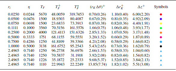


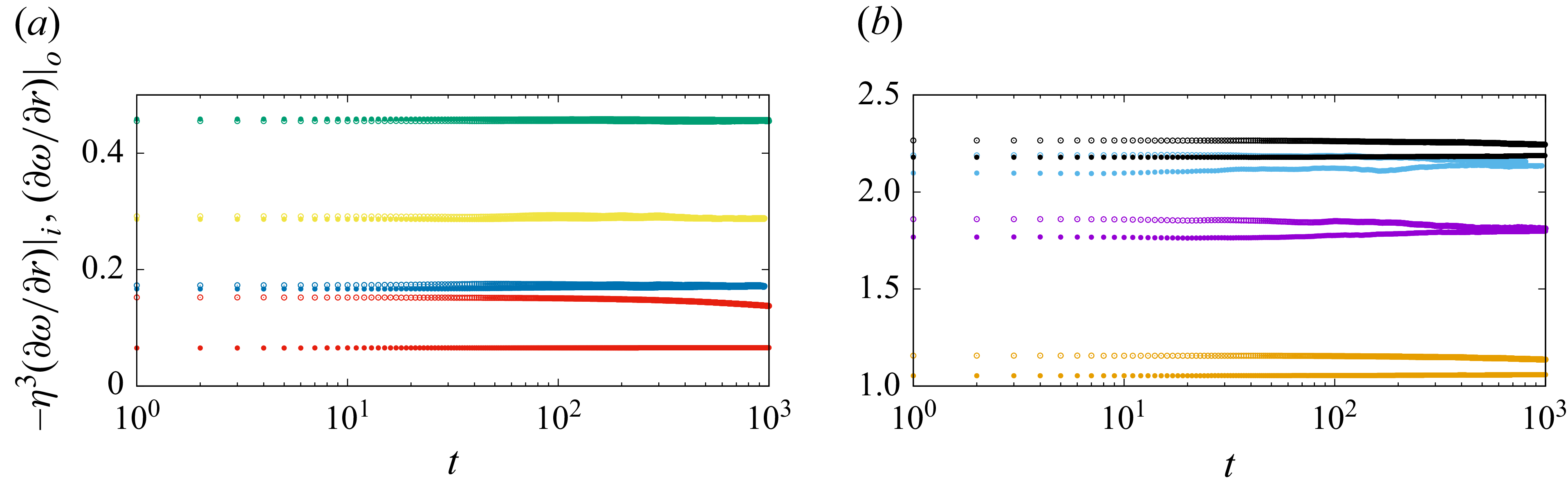


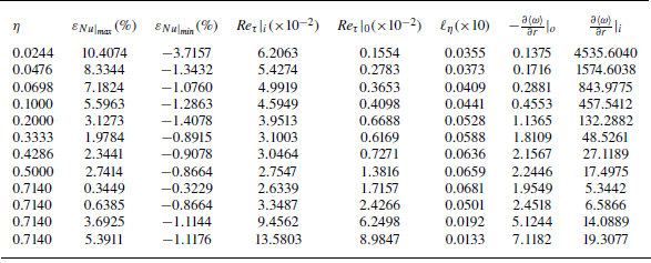


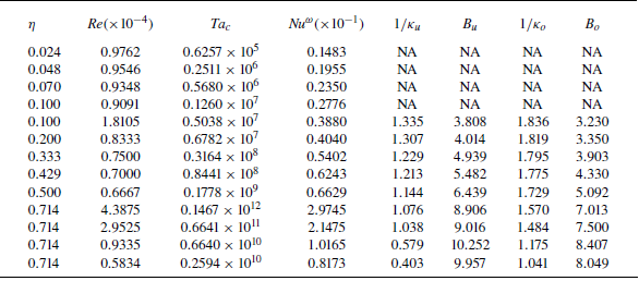


 Open access