


1. Introduction
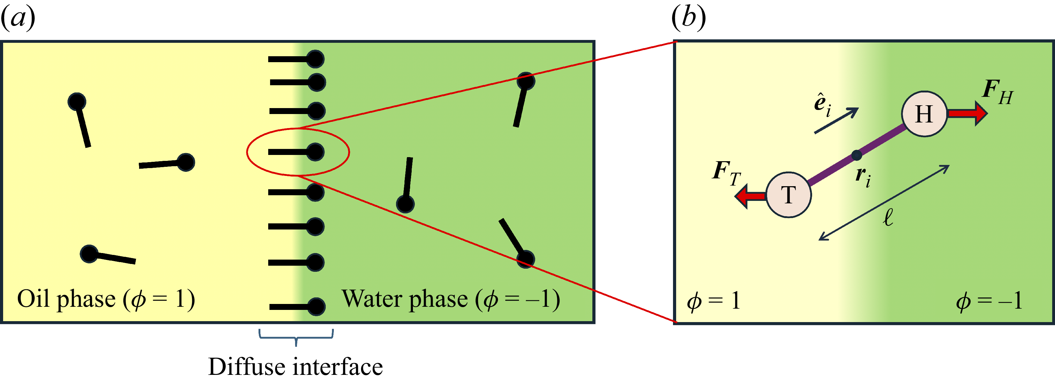
Systems containing surfactants are widely studied due to their numerous industrial applications, including in medicine, cleaning products and the food industry (Tadros Reference Tadros2005; Shaban, Kang & Kim Reference Shaban, Kang and Kim2020. Their primary utility lies in their ability to adsorb at fluid–fluid interfaces, such as liquid–gas or oil–water boundaries, where they reduce surface tension and inhibit droplet coalescence (Mulqueen & Blankschtein Reference Mulqueen and Blankschtein2002). For instance, in an emulsion of oil droplets dispersed in water, surfactants stabilise the droplet interfaces, thereby slowing the phase separation into two macroscopic oil and water phases. Surfactant molecules are amphiphilic, typically composed of a hydrophilic ‘head’ and a hydrophobic ‘tail’. The hydrophilic head is attracted to the water phase, while the hydrophobic tail prefers the oil phase, leading to an orientation that is perpendicular to the interface (as shown in figure 1 a). Upon adsorption at the interface, surfactants reduce the interfacial energy and thereby lower the surface tension. Once the interface becomes saturated, no further surfactant molecules can adsorb, causing the surface tension to level off (Touhami et al. Reference Touhami, Rana, Neale and Hornof2001; Wang et al. Reference Wang, Haghmoradi, Liu, Xi, Hirasaki, Miller and Chapman2017). Excess surfactants in the bulk phase may then self-assemble into micelles – spherical aggregates with hydrophobic tails hidden in the core and hydrophilic heads exposed to the surrounding fluid (Gangula, Suen & Conte Reference Gangula, Suen and Conte2010; Santos & Panagiotopoulos Reference Santos and Panagiotopoulos2016). Beyond surface tension reduction, surfactants also suppress droplet coalescence (Dai & Leal Reference Dai and Leal2008; Krebs, Schroën & Boom Reference Krebs, Schroën and Boom2012), thereby enhancing the stability and mixing of otherwise immiscible phases.
Previous theoretical treatments of ternary systems – comprising two immiscible fluids and a surfactant population – have included Ising-like lattice models (Alexander Reference Alexander1978; Ahluwalia & Puri Reference Ahluwalia and Puri1996), Potts models (Gilhøj et al. Reference Gilhøj, Laradji, Dammann, Jeppesen, Mouritsen, Toxvaerd and Zuckermann1996) and direct molecular dynamics simulations (Laradji & Mouritsen Reference Laradji and Mouritsen2000). Early continuum models either neglected the polarisation field entirely or integrated out its degrees of freedom from the dynamics (Kawasaki & Kawakatsu Reference Kawasaki and Kawakatsu1990; Anisimov et al. Reference Anisimov, Gorodetsky, Davydov and Kurliandsky1992). The first study to explicitly include the coarse-grained polarisation field dynamics (Melenkevitz & Javadpour Reference Melenkevitz and Javadpour1997) neglected both hydrodynamic interactions and thermal fluctuations. More recent continuum models of surfactant-covered binary fluids employ a free energy functional that depends on the surfactant concentration but omits the explicit dynamics of the polarisation field
 $\boldsymbol{p}(\boldsymbol{r},t)$
. Instead of incorporating
$\boldsymbol{p}(\boldsymbol{r},t)$
. Instead of incorporating
 $\boldsymbol{p}(\boldsymbol{r},t)$
, such models introduce additional stabilising terms to prevent the surfactant from destabilising the diffuse interface (Liu & Zhang Reference Liu and Zhang2010; Zhu et al. Reference Zhu, Kou, Yao, Li and Sun2020). These terms are often chosen to enforce Langmuir’s adsorption isotherm (Kalam et al. Reference Kalam, Abu-Khamsin, Kamal and Patil2021) and the Gibbs adsorption equation (Manikantan & Squires Reference Manikantan and Squires2020), which respectively govern surfactant uptake at interfaces and the relationship between surface tension and surfactant concentration. As a result, these models can successfully capture the reduction in surface tension with increasing surfactant concentration (Liu & Zhang Reference Liu and Zhang2010). Coupling the surfactant and order parameter fields to the fluid velocity field further allows these models to reproduce, to some extent, the suppression of droplet coalescence (Liu & Zhang Reference Liu and Zhang2010; Soligo et al. Reference Soligo, Roccon and Soldati2019a
,
Reference Soligo, Roccon and Soldatib
).
$\boldsymbol{p}(\boldsymbol{r},t)$
, such models introduce additional stabilising terms to prevent the surfactant from destabilising the diffuse interface (Liu & Zhang Reference Liu and Zhang2010; Zhu et al. Reference Zhu, Kou, Yao, Li and Sun2020). These terms are often chosen to enforce Langmuir’s adsorption isotherm (Kalam et al. Reference Kalam, Abu-Khamsin, Kamal and Patil2021) and the Gibbs adsorption equation (Manikantan & Squires Reference Manikantan and Squires2020), which respectively govern surfactant uptake at interfaces and the relationship between surface tension and surfactant concentration. As a result, these models can successfully capture the reduction in surface tension with increasing surfactant concentration (Liu & Zhang Reference Liu and Zhang2010). Coupling the surfactant and order parameter fields to the fluid velocity field further allows these models to reproduce, to some extent, the suppression of droplet coalescence (Liu & Zhang Reference Liu and Zhang2010; Soligo et al. Reference Soligo, Roccon and Soldati2019a
,
Reference Soligo, Roccon and Soldatib
).
(a) is a schematic diagram illustrating how surfactants (black) are absorbed perpendicularly at the interface between two phases, e.g. water and oil phase (green and yellow, respectively). (b) shows a diagram showing the surfactant molecule modelled as a dumbbell, adsorbed into a diffuse water–oil interface, with ‘head’ H, ‘tail’ T, rod of length
 $\ell$
, centre of mass
$\ell$
, centre of mass
 $\boldsymbol{r}_i$
and orientation vector
$\boldsymbol{r}_i$
and orientation vector
 $\hat {\boldsymbol{e}}_i$
, directed from ‘tail’ to ‘head’. The fluid exerts a force on each mass point,
$\hat {\boldsymbol{e}}_i$
, directed from ‘tail’ to ‘head’. The fluid exerts a force on each mass point,
 $\boldsymbol{F}_{\kern-1.5pt \textit{H}}$
and
$\boldsymbol{F}_{\kern-1.5pt \textit{H}}$
and
 $\boldsymbol{F}_{\textit{T}}$
, due to the hydrophilic/hydrophobic attraction between said mass points and the corresponding fluid phases. The binary fluid order parameter
$\boldsymbol{F}_{\textit{T}}$
, due to the hydrophilic/hydrophobic attraction between said mass points and the corresponding fluid phases. The binary fluid order parameter
 $\phi (\boldsymbol{r},t)$
has values between
$\phi (\boldsymbol{r},t)$
has values between
 $1$
and
$1$
and
 $-1$
to represent the two fluid phases.
$-1$
to represent the two fluid phases.
A wide range of numerical methods have been employed to directly simulate the continuum equations of diffuse interface systems, including finite volume (Yamashita, Matsushita & Suekane Reference Yamashita, Matsushita and Suekane2024) and finite difference schemes (Teigen et al. Reference Erik Teigen, Song, Lowengrub and Voigt2011), as well as more specialised computational approaches (Booty & Siegel Reference Booty and Siegel2010; Yang Reference Yang2021). Such simulations provide insights into the behaviour of surfactant-laden droplets under various conditions, including spinodal decomposition (Kim Reference Kim2006), shear flows (Teigen et al. Reference Erik Teigen, Song, Lowengrub and Voigt2011) and wetting dynamics (Ganesan Reference Ganesan2015). Alternative approaches to direct numerical simulation include lattice gas (Frisch, Hasslacher & Pomeau Reference Frisch, Hasslacher and Pomeau1986) and lattice Boltzmann methods (Higuera, Succi & Benzi Reference Higuera, Succi and Benzi1989; Benzi, Succi & Vergassola Reference Benzi, Succi and Vergassola1992), which were initially developed for binary fluid systems (Rothman & Keller Reference Rothman and Keller1988; Chan & Liang Reference Chan and Liang1990) and later extended to ternary mixtures, where surfactants act as a third component (Theissen & Gompper Reference Theissen and Gompper1999; Love et al. Reference Love, Nekovee, Coveney, Chin, González-Segredo and Martin2003; Kian Far et al. Reference Kian Far, Gorakifard and Fattahi2021). Lattice Boltzmann methods can be broadly classified as either free-energy-based methods or pseudopotential approaches (Krüger et al. Reference Krüger, Kusumaatmaja, Kuzmin, Shardt, Silva and Viggen2017). The pseudopotential approach mimics attractive or repulsive interactions between different species of fluid molecules, but does not have a direct connection to microscopic physics. To date, only pseudopotential-based models have been used to explicitly simulate the dynamics of the polarisation field associated with surfactant molecules – aside from Melenkevitz & Javadpour (Reference Melenkevitz and Javadpour1997), who neglected hydrodynamics.
In this work, we develop a continuum model of surfactant-laden binary fluids that is rigorously grounded in microscopic physics. Our central methodology is based on Rayleigh’s minimum energy dissipation principle, which we use to derive the overdamped dynamics of surfactant molecules interacting with a diffuse interface. This variational approach allows us to self-consistently obtain both the stochastic microscopic dynamics and, upon coarse-graining, the macroscopic hydrodynamic equations for the coupled fields: binary fluid volume fraction
 $\phi (\boldsymbol{r},t)$
, surfactant concentration
$\phi (\boldsymbol{r},t)$
, surfactant concentration
 $c(\boldsymbol{r},t)$
, polarisation
$c(\boldsymbol{r},t)$
, polarisation
 $\boldsymbol{p}(\boldsymbol{r},t)$
and fluid velocity
$\boldsymbol{p}(\boldsymbol{r},t)$
and fluid velocity
 $\boldsymbol{v}(\boldsymbol{r},t)$
. Unlike many previous models that introduce phenomenological terms to enforce stability or empirical adsorption laws, our formulation derives all equations from a single Rayleighian functional and a unified coarse-grained free energy, preserving detailed balance at equilibrium and ensuring thermodynamic consistency.
$\boldsymbol{v}(\boldsymbol{r},t)$
. Unlike many previous models that introduce phenomenological terms to enforce stability or empirical adsorption laws, our formulation derives all equations from a single Rayleighian functional and a unified coarse-grained free energy, preserving detailed balance at equilibrium and ensuring thermodynamic consistency.
A key advantage of this framework is that Marangoni flows arise naturally without the need to impose an additional surface-tension–gradient term. Because each surfactant exerts a tangential force on the interface, any spatial heterogeneity in surfactant concentration produces an excess stress that drives flow along the interface. The resulting long-ranged disturbances in the fluid velocity are therefore the exact analogue of the classical Marangoni flows generated by gradients in surface tension. Moreover, the model is thermodynamically consistent with both the Gibbs adsorption isotherm for surface-tension reduction and Henry’s law for the excess of surfactant at interfaces.
Assuming weak coupling between the fluid and surfactants allows us to obtain a perturbative equilibrium solution for a flat interface. We validate this analytical solution by numerically simulating the same planar interface using a hybrid finite-difference–pseudospectral method. This solution confirms that our model accurately captures the reduction in surface tension due to surfactant adsorption, in agreement with both previous phase-field models and experimental observations. We then perform numerical simulations of an emulsion to demonstrate how the inclusion of the polarisation field
 $\boldsymbol{p}(\boldsymbol{r},t)$
suppresses droplet coalescence. Previous studies have used pseudopotential-based methods to generate ultra-stable emulsions (Pelusi et al. Reference Pelusi, Lulli, Sbragaglia and Bernaschi2022). In contrast, our results show that stable emulsification can be achieved within a continuum framework, provided the surfactant polarisation dynamics is explicitly incorporated.
$\boldsymbol{p}(\boldsymbol{r},t)$
suppresses droplet coalescence. Previous studies have used pseudopotential-based methods to generate ultra-stable emulsions (Pelusi et al. Reference Pelusi, Lulli, Sbragaglia and Bernaschi2022). In contrast, our results show that stable emulsification can be achieved within a continuum framework, provided the surfactant polarisation dynamics is explicitly incorporated.
2. Microscopic derivation of the hydrodynamic equations
At the microscopic level, each surfactant molecule is modelled as a dumbbell composed of two mass points: a hydrophilic head (H) and a hydrophobic tail (T), connected by a rigid rod of length
 $\ell$
(Kawakatsu & Kawasaki Reference Kawakatsu and Kawasaki1990), see figure 1
b. The surrounding fluid is treated as a continuum, described by a velocity field
$\ell$
(Kawakatsu & Kawasaki Reference Kawakatsu and Kawasaki1990), see figure 1
b. The surrounding fluid is treated as a continuum, described by a velocity field
 $\boldsymbol{v}(\boldsymbol{r},t)$
and a volume fraction field
$\boldsymbol{v}(\boldsymbol{r},t)$
and a volume fraction field
 $\phi (\boldsymbol{r},t)$
. The field
$\phi (\boldsymbol{r},t)$
. The field
 $\phi (\boldsymbol{r},t)$
represents the local volume fraction of one component (e.g. oil) relative to the total volume of both components (oil and water), with
$\phi (\boldsymbol{r},t)$
represents the local volume fraction of one component (e.g. oil) relative to the total volume of both components (oil and water), with
 $\phi \gt 0$
indicating a local excess of component 1 and
$\phi \gt 0$
indicating a local excess of component 1 and
 $\phi \lt 0$
indicating a local excess of component 2. In this work, we take component 1 to be oil and component 2 to be water, although this labelling is arbitrary. Under appropriate conditions, a diffuse oil–water interface emerges, to which the surfactant molecules are attracted. In figure 1
b, the vector
$\phi \lt 0$
indicating a local excess of component 2. In this work, we take component 1 to be oil and component 2 to be water, although this labelling is arbitrary. Under appropriate conditions, a diffuse oil–water interface emerges, to which the surfactant molecules are attracted. In figure 1
b, the vector
 $\hat {\boldsymbol{e}}_i$
denotes the orientation of surfactant molecule
$\hat {\boldsymbol{e}}_i$
denotes the orientation of surfactant molecule
 $i$
, pointing from tail to head, with the centre of mass located at
$i$
, pointing from tail to head, with the centre of mass located at
 $\boldsymbol{r}_i$
. The head is attracted to the aqueous phase, while the tail prefers the oil phase. These preferential interactions generate a net force
$\boldsymbol{r}_i$
. The head is attracted to the aqueous phase, while the tail prefers the oil phase. These preferential interactions generate a net force
 $\boldsymbol{F}_i^{\textit{fluid}}$
and a net torque
$\boldsymbol{F}_i^{\textit{fluid}}$
and a net torque
 $\boldsymbol{T}_i^{\textit{fluid}}$
(about the centre of mass) when the molecule is not perpendicular with the interface or displaced from the midpoint of the interface. From figure 1
b,
$\boldsymbol{T}_i^{\textit{fluid}}$
(about the centre of mass) when the molecule is not perpendicular with the interface or displaced from the midpoint of the interface. From figure 1
b,
 $\boldsymbol{F}_i^{\textit{fluid}}$
and
$\boldsymbol{F}_i^{\textit{fluid}}$
and
 $\boldsymbol{T}_i^{\textit{fluid}}$
can be expressed as
$\boldsymbol{T}_i^{\textit{fluid}}$
can be expressed as
 \begin{align} \boldsymbol{F}_i^{\textit{fluid}} &= \boldsymbol{F}_{\kern-1.5pt \textit{H}} ( \boldsymbol{r}_i^+ ) + \boldsymbol{F}_{\textit{T}} ( \boldsymbol{r}_i^- ), \\[-10pt] \nonumber \end{align}
 \begin{align} \boldsymbol{T}_i^{\textit{fluid}} &= \frac {\ell }{2} \, \hat {\boldsymbol{e}}_i \times \boldsymbol{F}_{\kern-1.5pt \textit{H}}( \boldsymbol{r}_i^+ ) - \frac {\ell }{2}\, \hat {\boldsymbol{e}}_i \times \boldsymbol{F}_{\textit{T}} ( \boldsymbol{r}_i^- ), \end{align}
where
 $\boldsymbol{F}_{\kern-1.5pt \textit{H}} ( \boldsymbol{r}_i^+ )$
and
$\boldsymbol{F}_{\kern-1.5pt \textit{H}} ( \boldsymbol{r}_i^+ )$
and
 $\boldsymbol{F}_{\textit{T}} ( \boldsymbol{r}_i^- )$
are the forces acting from the fluid on the surfactant mass points H and T, respectively, with
$\boldsymbol{F}_{\textit{T}} ( \boldsymbol{r}_i^- )$
are the forces acting from the fluid on the surfactant mass points H and T, respectively, with
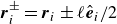 $\boldsymbol{r}_i^\pm = \boldsymbol{r}_i \pm \ell \hat {\boldsymbol{e}}_i/2$
denoting the positions of H (for
$\boldsymbol{r}_i^\pm = \boldsymbol{r}_i \pm \ell \hat {\boldsymbol{e}}_i/2$
denoting the positions of H (for
 $+$
) and T (for
$+$
) and T (for
 $-$
). The forces are obtained as
$-$
). The forces are obtained as
 \begin{align} \boldsymbol{F}_{\kern-1.5pt \textit{H}} (\boldsymbol{r}_i^+) &= -\chi \boldsymbol{\nabla }\phi (\boldsymbol{r})|_{\boldsymbol{r}=\boldsymbol{r}_i^+} , \\[-10pt] \nonumber \end{align}
 \begin{align} \boldsymbol{F}_{\textit{T}} (\boldsymbol{r}_i^-) &= +\chi \boldsymbol{\nabla }\phi (\boldsymbol{r})|_{\boldsymbol{r}=\boldsymbol{r}_i^-} , \end{align}
where
 $\boldsymbol{\nabla }\phi (\boldsymbol{r})|_{\boldsymbol{r}=\boldsymbol{r}_i^\pm }$
is the spatial derivative of
$\boldsymbol{\nabla }\phi (\boldsymbol{r})|_{\boldsymbol{r}=\boldsymbol{r}_i^\pm }$
is the spatial derivative of
 $\phi (\boldsymbol{r})$
, evaluated at
$\phi (\boldsymbol{r})$
, evaluated at
 $\boldsymbol{r}_i^\pm$
. In addition,
$\boldsymbol{r}_i^\pm$
. In addition,
 $\chi \gt 0$
is the interaction strength between each mass point and their preferential fluid phases (assumed to be equal in magnitude). Substituting (2.2) into (2.1), and Taylor expanding for small
$\chi \gt 0$
is the interaction strength between each mass point and their preferential fluid phases (assumed to be equal in magnitude). Substituting (2.2) into (2.1), and Taylor expanding for small
 $\ell$
, we obtain the net force and the net torque acting on each molecule
$\ell$
, we obtain the net force and the net torque acting on each molecule
 $i$
from the fluid:
$i$
from the fluid:
 \begin{align} \boldsymbol{F}_i^{\textit{fluid}} &= -\chi \ell (\hat {\boldsymbol{e}}_i\boldsymbol{\cdot }\boldsymbol{\nabla }_i)\boldsymbol{\nabla }_i\phi (\boldsymbol{r}_i) + \mathcal{O}(\ell ^2) , \\[-10pt] \nonumber \end{align}
 \begin{align} \boldsymbol{T}_i^{\textit{fluid}} &= -\chi \ell \hat {\boldsymbol{e}}_i\times \boldsymbol{\nabla }_i\phi (\boldsymbol{r}_i) + \mathcal{O}(\ell ^2), \end{align}
where
 $\boldsymbol{\nabla }_i$
indicates derivative with respect to
$\boldsymbol{\nabla }_i$
indicates derivative with respect to
 $\boldsymbol{r}_i$
, the centre of mass of molecule
$\boldsymbol{r}_i$
, the centre of mass of molecule
 $i$
. Motivated by the structure of the above-mentioned force and torque expressions, we derive the corresponding microscopic dynamics. From this microcopic dynamics, we can then obtain the coarse-grained hydrodynamic equations governing the coupled surfactant–binary fluid systems.
$i$
. Motivated by the structure of the above-mentioned force and torque expressions, we derive the corresponding microscopic dynamics. From this microcopic dynamics, we can then obtain the coarse-grained hydrodynamic equations governing the coupled surfactant–binary fluid systems.
2.1. Rayleighian dissipation for a single surfactant molecule in a binary fluid
In this section, we first derive the microscopic dynamics of a single surfactant molecule in a binary fluid using Rayleigh’s minimum energy dissipation principle (Doi Reference Doi2011, Reference Doi2013). We then extend this framework to an ensemble of non-interacting surfactant molecules by introducing a single-particle distribution function. This allows us to derive the coarse-grained hydrodynamic equations in terms of the concentration field
 $c(\boldsymbol{r},t)$
, polarisation field
$c(\boldsymbol{r},t)$
, polarisation field
 $\boldsymbol{p}(\boldsymbol{r},t)$
, binary fluid volume fraction field
$\boldsymbol{p}(\boldsymbol{r},t)$
, binary fluid volume fraction field
 $\phi (\boldsymbol{r},t)$
and velocity field
$\phi (\boldsymbol{r},t)$
and velocity field
 $\boldsymbol{v}(\boldsymbol{r},t)$
.
$\boldsymbol{v}(\boldsymbol{r},t)$
.
We first consider a system of a single dumbbell with two point masses at
 $\boldsymbol{r}^+$
and
$\boldsymbol{r}^+$
and
 $\boldsymbol{r}^-$
, representing the positions of the head and the tail, respectively. We also have
$\boldsymbol{r}^-$
, representing the positions of the head and the tail, respectively. We also have
 $|\boldsymbol{r}^+-\boldsymbol{r}^-|= \ell$
, where
$|\boldsymbol{r}^+-\boldsymbol{r}^-|= \ell$
, where
 $\ell$
is the length of the dumbbell. The free energy of a single dumbbell particle in a continuum fluid is then given by
$\ell$
is the length of the dumbbell. The free energy of a single dumbbell particle in a continuum fluid is then given by
 \begin{align} A[\phi ,\{\boldsymbol{r}^+,\boldsymbol{r}^-\}] = F_{\textit{fluid}}[\phi ] + \int d^dr \, \left \{ \chi \left [\delta (\boldsymbol{r}-\boldsymbol{r}^+) - \delta (\boldsymbol{r}-\boldsymbol{r}^-)\right ] \phi (\boldsymbol{r}) \right \}, \end{align}
where
 \begin{align} F_{\textit{fluid}}[\phi ]=\int d^dr \left \{ \frac {\alpha }{2}\phi ^2 + \frac {\beta }{4}\phi ^4 + \frac {\kappa }{2}|\boldsymbol{\nabla }\phi |^2 \right \} \end{align}
is a typical free energy of a binary fluid, containing a double-well potential (for
 $\alpha \lt 0$
and
$\alpha \lt 0$
and
 $\beta \gt 0$
) to drive bulk phase separation which competes with a squared-gradient term to penalise surface proliferation. Here, we take
$\beta \gt 0$
) to drive bulk phase separation which competes with a squared-gradient term to penalise surface proliferation. Here, we take
 $\alpha =-\beta \lt 0$
, so that equilibrium phases correspond to
$\alpha =-\beta \lt 0$
, so that equilibrium phases correspond to
 $\phi =\pm \sqrt {-\alpha /\beta }=\pm 1$
. Note that
$\phi =\pm \sqrt {-\alpha /\beta }=\pm 1$
. Note that
 $d$
is the spatial dimension and the integral is taken over the volume of the system. The second term in (2.4) couples the two discrete head and tail positions to the volume fraction field, with each particle–field interaction characterised by an interaction strength
$d$
is the spatial dimension and the integral is taken over the volume of the system. The second term in (2.4) couples the two discrete head and tail positions to the volume fraction field, with each particle–field interaction characterised by an interaction strength
 $\chi$
(Hardy, Daddi-Moussa-Ider & Tjhung Reference Hardy, Daddi-Moussa-Ider and Tjhung2024). We now introduce the orientation unit vector
$\chi$
(Hardy, Daddi-Moussa-Ider & Tjhung Reference Hardy, Daddi-Moussa-Ider and Tjhung2024). We now introduce the orientation unit vector
 $\hat {\boldsymbol{e}}$
and the centre of mass position
$\hat {\boldsymbol{e}}$
and the centre of mass position
 $\boldsymbol{R}$
to be
$\boldsymbol{R}$
to be
 \begin{align} \hat {\boldsymbol{e}} = \frac {\boldsymbol{r}^+-\boldsymbol{r}^-}{\ell } \quad \text{and}\quad \boldsymbol{R} &= \frac {\boldsymbol{r}^++\boldsymbol{r}^-}{2}. \end{align}
Then, (2.4) becomes
 \begin{align} A[\phi ,\{\boldsymbol{R},\hat {\boldsymbol{e}}\}] = F_{\textit{fluid}}[\phi ] + \!\!\int\! d^dr \left \{ \chi \left [\delta \left (\boldsymbol{r}-\left (\boldsymbol{R}+\frac {\ell }{2}\hat {\boldsymbol{e}}\right )\right ) \!-\! \delta \left (\boldsymbol{r}-\left (\boldsymbol{R}-\frac {\ell }{2}\hat {\boldsymbol{e}}\right )\right ) \right ] \phi (\boldsymbol{r}) \! \right \}\!. \end{align}
Taylor expanding (2.7) for small
 $\ell$
, we may obtain
$\ell$
, we may obtain
 \begin{align} A[\phi ,\{\boldsymbol{R},\hat {\boldsymbol{e}}\}] = F_{\textit{fluid}}[\phi ] + \chi \ell (\hat {\boldsymbol{e}}\boldsymbol{\cdot }\boldsymbol{\nabla }_{\boldsymbol{R}})\phi (\boldsymbol{R}) + \mathcal{O}(\ell ^3), \end{align}
where
 $\boldsymbol{\nabla }_{\boldsymbol{R}}$
denotes spatial derivative with respect to the centre of mass of the dumbbell
$\boldsymbol{\nabla }_{\boldsymbol{R}}$
denotes spatial derivative with respect to the centre of mass of the dumbbell
 $\boldsymbol{R}$
. Thus, the hybrid discrete-particle–continuum-fluid free energy is a functional of the volume fraction field
$\boldsymbol{R}$
. Thus, the hybrid discrete-particle–continuum-fluid free energy is a functional of the volume fraction field
 $\phi (\boldsymbol{r})$
and a function of discrete variables
$\phi (\boldsymbol{r})$
and a function of discrete variables
 $\boldsymbol{R}$
and
$\boldsymbol{R}$
and
 $\hat {\boldsymbol{e}}$
. Ultimately, we aim to re-cast (2.7) or (2.8) as a purely continuum free energy.
$\hat {\boldsymbol{e}}$
. Ultimately, we aim to re-cast (2.7) or (2.8) as a purely continuum free energy.
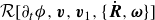
Following Doi (Reference Doi2011), we next write down the Rayleigh dissipation functional
 \begin{align} \mathcal{R}[\partial _t\phi ,\boldsymbol{v}_1,\boldsymbol{v}_2,\{\dot {\boldsymbol{r}}^+,\dot {\boldsymbol{r}}^-\}] = \varPhi _1[\boldsymbol{v}] + \varPhi _2[\boldsymbol{v}_1,\boldsymbol{v}_2] + \varPhi _3[\boldsymbol{v},\{\dot {\boldsymbol{r}}^+,\dot {\boldsymbol{r}}^-\}]+ \dot {A} , \end{align}
which is a functional of the rate of change of the volume fraction
 $\partial _t\phi$
; the velocity of fluid component 1,
$\partial _t\phi$
; the velocity of fluid component 1,
 $\boldsymbol{v}_1(\boldsymbol{r},t)$
; the velocity of fluid component 2,
$\boldsymbol{v}_1(\boldsymbol{r},t)$
; the velocity of fluid component 2,
 $\boldsymbol{v}_2(\boldsymbol{r},t)$
; and the velocities of the discrete particles
$\boldsymbol{v}_2(\boldsymbol{r},t)$
; and the velocities of the discrete particles
 $\{\dot {\boldsymbol{r}}^+,\dot {\boldsymbol{r}}^-\}$
. We may also further define the total velocity of the fluid to be
$\{\dot {\boldsymbol{r}}^+,\dot {\boldsymbol{r}}^-\}$
. We may also further define the total velocity of the fluid to be
 \begin{align} \boldsymbol{v}(\boldsymbol{r},t)=\frac {1+\phi }{2}\boldsymbol{v}_1(\boldsymbol{r},t)+\frac {1-\phi }{2}\boldsymbol{v}_2(\boldsymbol{r},t), \end{align}
so that either
 $\boldsymbol{v}_1$
or
$\boldsymbol{v}_1$
or
 $\boldsymbol{v}_2$
may be expressed in terms of
$\boldsymbol{v}_2$
may be expressed in terms of
 $\boldsymbol{v}$
and the other. We use a dot over any variable to denote its total time-derivative. We neglect the volume of discrete particles in this formulation. The first dissipation term in (2.9) denotes the viscous dissipation of the incompressible Newtonian fluid,
$\boldsymbol{v}$
and the other. We use a dot over any variable to denote its total time-derivative. We neglect the volume of discrete particles in this formulation. The first dissipation term in (2.9) denotes the viscous dissipation of the incompressible Newtonian fluid,
 \begin{align} \varPhi _1[\boldsymbol{v}] = \int d^dr \, \frac {\eta }{4} \big [\boldsymbol{\nabla }\boldsymbol{v}+(\boldsymbol{\nabla }\boldsymbol{v})^T\big ]^2 - \int d^dr \, P(\boldsymbol{r}) \boldsymbol{\nabla }\boldsymbol{\cdot }\boldsymbol{v}, \end{align}
where
 $\eta$
is the fluid viscosity (assumed to be the same for both components of the fluid) and
$\eta$
is the fluid viscosity (assumed to be the same for both components of the fluid) and
 $P(\boldsymbol{r})$
is a Lagrange multiplier to enforce incompressibility condition
$P(\boldsymbol{r})$
is a Lagrange multiplier to enforce incompressibility condition
 $\boldsymbol{\nabla }\boldsymbol{\cdot }\boldsymbol{v}=0$
, which also happens to be the pressure of the fluid. The second dissipation term in (2.9) represents dissipation due to velocity differences between the two fluid components,
$\boldsymbol{\nabla }\boldsymbol{\cdot }\boldsymbol{v}=0$
, which also happens to be the pressure of the fluid. The second dissipation term in (2.9) represents dissipation due to velocity differences between the two fluid components,
 \begin{align} \varPhi _2[\boldsymbol{v}_1,\boldsymbol{v}_2] =\int d^dr \, \frac {\xi }{2} (\boldsymbol{v}_1-\boldsymbol{v}_2)^2 = \int d^dr \, \frac {2\xi }{(1-\phi )^2}(\boldsymbol{v}_1-\boldsymbol{v})^2, \end{align}
where
 $\xi \gt 0$
is a phenomenological dissipation parameter related to the mobility. The third term in (2.9) couples the fluid velocity to the particle velocities
$\xi \gt 0$
is a phenomenological dissipation parameter related to the mobility. The third term in (2.9) couples the fluid velocity to the particle velocities
 \begin{align} \varPhi _3[\boldsymbol{v},\{\dot {\boldsymbol{r}}^+,\dot {\boldsymbol{r}}^-\}] = - \!\int\! d^dr \left \{ \delta (\boldsymbol{r}-\boldsymbol{r}^+)\boldsymbol{f}^+\boldsymbol{\cdot }(\boldsymbol{v}(\boldsymbol{r})-\dot {\boldsymbol{r}}^+) + \delta (\boldsymbol{r}-\boldsymbol{r}^-)\boldsymbol{f}^-\boldsymbol{\cdot }(\boldsymbol{v}(\boldsymbol{r})-\dot {\boldsymbol{r}}^-) \right \}\!, \end{align}
where
 $\boldsymbol{f}^\pm$
are constraint forces which enforce
$\boldsymbol{f}^\pm$
are constraint forces which enforce
 $\boldsymbol{v}(\boldsymbol{r}^\pm )=\dot {\boldsymbol{r}}^\pm$
(similar to Lagrange multipliers). This is equivalent to introducing point forces acting on the fluid (i.e. Stokeslet solution). We can define the angular velocity of the dumbbell
$\boldsymbol{v}(\boldsymbol{r}^\pm )=\dot {\boldsymbol{r}}^\pm$
(similar to Lagrange multipliers). This is equivalent to introducing point forces acting on the fluid (i.e. Stokeslet solution). We can define the angular velocity of the dumbbell
 $\boldsymbol{\omega }$
to be
$\boldsymbol{\omega }$
to be
 $\dot {\hat {\boldsymbol{e}}}=\boldsymbol{\omega }\times \hat {\boldsymbol{e}}$
. The rate of change of the positions
$\dot {\hat {\boldsymbol{e}}}=\boldsymbol{\omega }\times \hat {\boldsymbol{e}}$
. The rate of change of the positions
 $\dot {\boldsymbol{r}}^\pm$
can then be written in terms of
$\dot {\boldsymbol{r}}^\pm$
can then be written in terms of
 $\dot {\boldsymbol{R}}$
and
$\dot {\boldsymbol{R}}$
and
 $\boldsymbol{\omega }$
:
$\boldsymbol{\omega }$
:
 \begin{align} \dot {\boldsymbol{r}}^\pm = \dot {\boldsymbol{R}} \pm \boldsymbol{\omega }\times \frac {\ell }{2}\hat {\boldsymbol{e}}. \end{align}
Using (2.14), (2.13) can then be written in terms of
 $\dot {\boldsymbol{R}}$
and
$\dot {\boldsymbol{R}}$
and
 $\boldsymbol{\omega }$
, and thus,
$\boldsymbol{\omega }$
, and thus,
 $\varPhi _3[\boldsymbol{v},\{\dot {\boldsymbol{R}},\boldsymbol{\omega }\}]$
is now a function of
$\varPhi _3[\boldsymbol{v},\{\dot {\boldsymbol{R}},\boldsymbol{\omega }\}]$
is now a function of
 $\dot {\boldsymbol{R}}$
and
$\dot {\boldsymbol{R}}$
and
 $\boldsymbol{\omega }$
. The final term in (2.9) is simply the derivative of the free energy with time,
$\boldsymbol{\omega }$
. The final term in (2.9) is simply the derivative of the free energy with time,
 \begin{eqnarray} \dot {A}[\partial _t\phi ,\{\dot {\boldsymbol{R}},\boldsymbol{\omega }\}] &=& \int d^dr \left \{ \frac {\delta F_{\textit{fluid}}}{\delta \phi } \partial _t\phi \right \} \nonumber\\ && +\, \int d^dr \left \{ \chi \partial _t\phi \left [ \delta \left (\boldsymbol{r}-\left (\boldsymbol{R}+\frac {\ell }{2}\hat {\boldsymbol{e}}\right )\right ) - \delta \left (\boldsymbol{r}-\left (\boldsymbol{R}-\frac {\ell }{2}\hat {\boldsymbol{e}}\right )\right ) \right ] \right \} \nonumber\\ && +\, \chi \left [ \boldsymbol{\nabla }\phi (\boldsymbol{r})|_{\boldsymbol{r}=\boldsymbol{R}+\ell \hat {\boldsymbol{e}}/2} - \boldsymbol{\nabla }\phi (\boldsymbol{r})|_{\boldsymbol{r}=\boldsymbol{R}-\ell \hat {\boldsymbol{e}}/2} \right ] \boldsymbol{\cdot }\dot {\boldsymbol{R}} \nonumber\\ && +\,\frac {\ell \chi }{2} \left [ \boldsymbol{\nabla }\phi (\boldsymbol{r})|_{\boldsymbol{r}=\boldsymbol{R}+\ell \hat {\boldsymbol{e}}/2} + \boldsymbol{\nabla }\phi (\boldsymbol{r})|_{\boldsymbol{r}=\boldsymbol{R}-\ell \hat {\boldsymbol{e}}/2} \right ] \boldsymbol{\cdot }\boldsymbol{\omega }\times \hat {\boldsymbol{e}}, \end{eqnarray}
where we have expressed
 $\dot {\hat {\boldsymbol{e}}}=\boldsymbol{\omega }\times \hat {\boldsymbol{e}}$
. Minimising the Rayleighian
$\dot {\hat {\boldsymbol{e}}}=\boldsymbol{\omega }\times \hat {\boldsymbol{e}}$
. Minimising the Rayleighian
 $\mathcal{R}[\partial _t\phi ,\boldsymbol{v},\boldsymbol{v}_1,\{\dot {\boldsymbol{R}},\boldsymbol{\omega }\}]$
with respect to the generalised velocities
$\mathcal{R}[\partial _t\phi ,\boldsymbol{v},\boldsymbol{v}_1,\{\dot {\boldsymbol{R}},\boldsymbol{\omega }\}]$
with respect to the generalised velocities
 $\partial _t\phi$
,
$\partial _t\phi$
,
 $\boldsymbol{v}$
,
$\boldsymbol{v}$
,
 $\boldsymbol{v}_1$
,
$\boldsymbol{v}_1$
,
 $\dot {\boldsymbol{R}}$
and
$\dot {\boldsymbol{R}}$
and
 $\boldsymbol{\omega }$
, and subject to the constraint that volume fraction is conserved, i.e.
$\boldsymbol{\omega }$
, and subject to the constraint that volume fraction is conserved, i.e.
 \begin{align} \partial _t\phi + \boldsymbol{\nabla }\boldsymbol{\cdot }[(1+\phi )\boldsymbol{v}_1] = 0, \end{align}
we get the equations of motion for the system:
 \begin{align} \partial _t\phi & = -\boldsymbol{v}\boldsymbol{\cdot }\boldsymbol{\nabla }\phi + M{\nabla} ^2\bigg (\frac {\delta A}{\delta \phi }\bigg ) , \\[-10pt] \nonumber \end{align}
 \begin{align} \boldsymbol{v}(\boldsymbol{r}) & = \int d^dr' \left [ \boldsymbol{O}(\boldsymbol{r}-\boldsymbol{r}') \boldsymbol{\cdot }\left (-\phi (\boldsymbol{r}')\boldsymbol{\nabla }'\frac {\delta A}{\delta \phi (\boldsymbol{r}')}\right ) \right ] \nonumber \\ & \quad +\, \left [ \boldsymbol{O}(\boldsymbol{r}-\boldsymbol{R}) + \frac {\ell ^2}{8}(\hat {\boldsymbol{e}}\hat {\boldsymbol{e}}:\boldsymbol{\nabla }_{\boldsymbol{R}}\boldsymbol{\nabla }_{\boldsymbol{R}}) \boldsymbol{O}(\boldsymbol{r}-\boldsymbol{R})\right ] \boldsymbol{\cdot }\boldsymbol{g} \nonumber \\ & \quad +\, \left [ (\boldsymbol{e}\boldsymbol{\cdot }\boldsymbol{\nabla }_{\boldsymbol{R}})\boldsymbol{O}(\boldsymbol{r}-\boldsymbol{R}) + \frac {\ell ^2}{3!}(\hat {\boldsymbol{e}}\hat {\boldsymbol{e}}\hat {\boldsymbol{e}}:\boldsymbol{\nabla }_{\boldsymbol{R}}\boldsymbol{\nabla }_{\boldsymbol{R}}\boldsymbol{\nabla }_{\boldsymbol{R}})\boldsymbol{O}(\boldsymbol{r}-\boldsymbol{R}) \right ]\boldsymbol{\cdot }\boldsymbol{h}+\mathcal{O}(\ell ^3) \\[-10pt] \nonumber \end{align}
 \begin{align} \boldsymbol{g} &=-\ell \chi (\hat {\boldsymbol{e}}\boldsymbol{\cdot }\boldsymbol{\nabla }_{\boldsymbol{R}})\boldsymbol{\nabla }_{\boldsymbol{R}}\phi (\boldsymbol{R}) + \mathcal{O}(\ell ^3), \\[-10pt] \nonumber \end{align}
 \begin{align} \boldsymbol{h} &=-\ell \chi \boldsymbol{\nabla }_{\boldsymbol{R}}\phi (\boldsymbol{R}) + \mathcal{O}(\ell ^3), \\[-10pt] \nonumber \end{align}
 \begin{align} \dot {\boldsymbol{R}} &= \boldsymbol{v}(\boldsymbol{R})+\mathcal{O}(\ell ^2), \\[-10pt] \nonumber \end{align}
 \begin{align} \dot {\hat {\boldsymbol{e}}} &= (\hat {\boldsymbol{e}}\boldsymbol{\cdot }\boldsymbol{\nabla }_{\boldsymbol{R}})\boldsymbol{v}(\boldsymbol{R})+\mathcal{O}(\ell ^2), \\[10pt] \nonumber \end{align}
where we have defined
 $\boldsymbol{g} = \boldsymbol{f}_{2}+\boldsymbol{f}_{1}$
and
$\boldsymbol{g} = \boldsymbol{f}_{2}+\boldsymbol{f}_{1}$
and
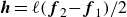 $\boldsymbol{h} = \ell (\boldsymbol{f}_{2}{-}\boldsymbol{f}_{1})/2$
. Here,
$\boldsymbol{h} = \ell (\boldsymbol{f}_{2}{-}\boldsymbol{f}_{1})/2$
. Here,
 $\boldsymbol{O}(\boldsymbol{r})$
is the second rank Oseen tensor, which in three dimensions (
$\boldsymbol{O}(\boldsymbol{r})$
is the second rank Oseen tensor, which in three dimensions (
 $d=3$
), is given by
$d=3$
), is given by
 \begin{align} \boldsymbol{O}(\boldsymbol{r})=\frac {1}{8\pi \eta r}\bigg (\boldsymbol{I}+\frac {\boldsymbol{r}\boldsymbol{r}}{r^2}\bigg ), \end{align}
where
 $\boldsymbol{I}$
is the identity matrix. To obtain (2.17), we have assumed that the binary fluid dissipation coefficient,
$\boldsymbol{I}$
is the identity matrix. To obtain (2.17), we have assumed that the binary fluid dissipation coefficient,
 $\xi \equiv (1+\phi )^2(1-\phi )^2 / (4M)$
, depends explicitly on the volume fraction, so that the mobility
$\xi \equiv (1+\phi )^2(1-\phi )^2 / (4M)$
, depends explicitly on the volume fraction, so that the mobility
 $M$
in (2.17a
) remains constant.
$M$
in (2.17a
) remains constant.
The singular nature of
 $\boldsymbol{O}(\boldsymbol{r})$
at
$\boldsymbol{O}(\boldsymbol{r})$
at
 $\boldsymbol{r}=\boldsymbol{0}$
poses a problem, as the centre-of-mass and orientation dynamics both require evaluating
$\boldsymbol{r}=\boldsymbol{0}$
poses a problem, as the centre-of-mass and orientation dynamics both require evaluating
 $\boldsymbol{v}(\boldsymbol{R})$
. However, there is a precedent in the literature to remedy this, particularly in polymer physics when one deals with strings of spherical beads (Doi & Edwards Reference Doi and Edwards1986). One can begin by assuming the singular term in the velocity dynamics is omitted. We will denote the remaining external flow velocity as
$\boldsymbol{v}(\boldsymbol{R})$
. However, there is a precedent in the literature to remedy this, particularly in polymer physics when one deals with strings of spherical beads (Doi & Edwards Reference Doi and Edwards1986). One can begin by assuming the singular term in the velocity dynamics is omitted. We will denote the remaining external flow velocity as
 $\boldsymbol{v}_{\textit{ext}}(\boldsymbol{r})$
, defined simply as
$\boldsymbol{v}_{\textit{ext}}(\boldsymbol{r})$
, defined simply as
 \begin{eqnarray} \boldsymbol{v}_{\textit{ext}}(\boldsymbol{r}) = \int d^dr' \left [ \boldsymbol{O}(\boldsymbol{r}-\boldsymbol{r}')\boldsymbol{\cdot }\left (-\phi (\boldsymbol{r}')\boldsymbol{\nabla '}\frac {\delta A}{\delta \phi (\boldsymbol{r}')} \right ) \right ] +\mathcal{O}(\ell ^3). \end{eqnarray}
To compensate for the neglect of the singular self-interaction flow, one needs to supplement the equations of
 $\dot {\boldsymbol{R}}$
and
$\dot {\boldsymbol{R}}$
and
 $\dot {\hat {\boldsymbol{e}}}$
by a self-interaction term, which is taken ad hoc to be the mobility matrix of the isolated particle multiplied by the force on that particle (neglecting hydrodynamic forces). For us, we choose the mobility matrix which is consistent with an isolated needle-like particle, as that is the closest to our dipolar case for which an exact solution is available. Then,
$\dot {\hat {\boldsymbol{e}}}$
by a self-interaction term, which is taken ad hoc to be the mobility matrix of the isolated particle multiplied by the force on that particle (neglecting hydrodynamic forces). For us, we choose the mobility matrix which is consistent with an isolated needle-like particle, as that is the closest to our dipolar case for which an exact solution is available. Then,
 \begin{align} \dot {\hat {\boldsymbol{e}}} &= \left (\boldsymbol{I}- \hat {\boldsymbol{e}}\hat {\boldsymbol{e}}\right ) \boldsymbol{\cdot }\left [ (\hat {\boldsymbol{e}}\boldsymbol{\cdot }\boldsymbol{\nabla }_{\boldsymbol{R}})\boldsymbol{v}_{\textit{ext}}(\boldsymbol{R}) - \frac {1}{\gamma _r}\frac {\partial A}{\partial \hat {\boldsymbol{e}}} \right ], \\[-10pt] \nonumber \end{align}
 \begin{align} \dot {\boldsymbol{R}} &= \boldsymbol{v}_{\textit{ext}}(\boldsymbol{R}) - \left [ \frac {1}{\zeta _{\parallel }} \hat {\boldsymbol{e}}\hat {\boldsymbol{e}} + \frac {1}{\zeta _{\perp }} \left ( \boldsymbol{I} - \hat {\boldsymbol{e}}\hat {\boldsymbol{e}} \right ) \right ] \boldsymbol{\cdot }\frac {\partial A}{\partial \boldsymbol{R}}. \end{align}
The operator
 $(\boldsymbol{I}-\hat {\boldsymbol{e}}\hat {\boldsymbol{e}})$
is known as the perpendicular projection operator, as it projects any vector
$(\boldsymbol{I}-\hat {\boldsymbol{e}}\hat {\boldsymbol{e}})$
is known as the perpendicular projection operator, as it projects any vector
 $\boldsymbol{V}$
onto the plane perpendicular to
$\boldsymbol{V}$
onto the plane perpendicular to
 $\hat {\boldsymbol{e}}$
, i.e.
$\hat {\boldsymbol{e}}$
, i.e.
 $(\boldsymbol{I}-\hat {\boldsymbol{e}}\hat {\boldsymbol{e}})\boldsymbol{\cdot }\boldsymbol{V}$
. We employ this operator in (2.20a
) to ensure that the unit-length constraint
$(\boldsymbol{I}-\hat {\boldsymbol{e}}\hat {\boldsymbol{e}})\boldsymbol{\cdot }\boldsymbol{V}$
. We employ this operator in (2.20a
) to ensure that the unit-length constraint
 $|\hat {\boldsymbol{e}}|=1$
is maintained throughout the dynamics. In (2.20),
$|\hat {\boldsymbol{e}}|=1$
is maintained throughout the dynamics. In (2.20),
 $\gamma _r$
is the rotational friction, and
$\gamma _r$
is the rotational friction, and
 $\zeta _{\parallel }$
and
$\zeta _{\parallel }$
and
 $\zeta _{\perp }$
are the translational friction parallel and perpendicular to
$\zeta _{\perp }$
are the translational friction parallel and perpendicular to
 $\hat {\boldsymbol{e}}$
, respectively. In the case of ellipsoidal particles, these friction coefficients can be written in terms of microscopic parameters (Kim & Karrila Reference Kim and Karrila2005); Hoffmann et al. Reference Hoffmann, Wagner, Harnau and Wittemann2009). This result reproduces the Jeffrey orbits if we define the symmetric and anti-symmetric tensors
$\hat {\boldsymbol{e}}$
, respectively. In the case of ellipsoidal particles, these friction coefficients can be written in terms of microscopic parameters (Kim & Karrila Reference Kim and Karrila2005); Hoffmann et al. Reference Hoffmann, Wagner, Harnau and Wittemann2009). This result reproduces the Jeffrey orbits if we define the symmetric and anti-symmetric tensors
 \begin{align} (\boldsymbol{D}_{\textit{ext}})_{\alpha \beta } \equiv & \frac {1}{2} \left [(\boldsymbol{\nabla })_{\alpha }(\boldsymbol{v}_{\textit{ext}})_{\beta } + (\boldsymbol{\nabla })_{\beta }(\boldsymbol{v}_{\textit{ext}})_{\alpha }\right ], \\[-10pt] \nonumber \end{align}
 \begin{align} (\boldsymbol{\varOmega }_{\textit{ext}})_{\alpha \beta } \equiv & \frac {1}{2} \left [(\boldsymbol{\nabla })_{\alpha }(\boldsymbol{v}_{\textit{ext}})_{\beta }-(\boldsymbol{\nabla })_{\beta }(\boldsymbol{v}_{\textit{ext}})_{\alpha }\right ], \end{align}
i.e.
 \begin{align} \dot {\hat {\boldsymbol{e}}} = \underbrace {-\boldsymbol{\varOmega }_{\textit{ext}}(\boldsymbol{R}) \boldsymbol{\cdot }\hat {\boldsymbol{e}} +B\left [\boldsymbol{D}_{\textit{ext}}(\boldsymbol{R}) \boldsymbol{\cdot }\hat {\boldsymbol{e}} - \left (\hat {\boldsymbol{e}}\boldsymbol{\cdot }\boldsymbol{D}_{\textit{ext}}(\boldsymbol{R}) \boldsymbol{\cdot }\hat {\boldsymbol{e}}\right )\hat {\boldsymbol{e}}\right ]}_{ \left (\boldsymbol{I}- \hat {\boldsymbol{e}}\hat {\boldsymbol{e}}\right ) \boldsymbol{\cdot }(\hat {\boldsymbol{e}}\boldsymbol{\cdot }\boldsymbol{\nabla }_{\boldsymbol{R}}) \boldsymbol{v}_{\textit{ext}}(\boldsymbol{R}) \text{ for } B=1} - \left (\boldsymbol{I}-\hat {\boldsymbol{e}}\hat {\boldsymbol{e}}\right ) \boldsymbol{\cdot }\bigg (\frac {1}{\gamma _r}\frac {\partial A}{\partial \hat {\boldsymbol{e}}}\bigg ), \end{align}
though we specifically have
 $B=1$
since we assumed the surfactant had a needle-like aspect ratio in our derivation. In the case of ellipsoidal particles,
$B=1$
since we assumed the surfactant had a needle-like aspect ratio in our derivation. In the case of ellipsoidal particles,
 $B$
is related to the aspect ratio of the particle
$B$
is related to the aspect ratio of the particle
 $\varDelta$
via
$\varDelta$
via
 $B=(\varDelta ^2-1)/(\varDelta ^2+1)$
(Jeffery Reference Jeffery1922). Up to this point, we have derived the dynamics of a single surfactant molecule in the presence of a phase-separating binary fluid, (2.20a
), (2.20b
) and (2.22), subject to external flow due to phase separation, (2.19).
$B=(\varDelta ^2-1)/(\varDelta ^2+1)$
(Jeffery Reference Jeffery1922). Up to this point, we have derived the dynamics of a single surfactant molecule in the presence of a phase-separating binary fluid, (2.20a
), (2.20b
) and (2.22), subject to external flow due to phase separation, (2.19).
Finally, we introduce noise to the single particle dynamics to get the Ito stochastic differential equations (in
 $d$
dimension),
$d$
dimension),
 \begin{align} d\boldsymbol{R} = &\left \{ \boldsymbol{v}_{\textit{ext}}(\boldsymbol{R}) -\left [ \frac {1}{\zeta _{\parallel }} \hat {\boldsymbol{e}}\hat {\boldsymbol{e}} + \frac {1}{\zeta _{\perp }}\left ( \boldsymbol{I}- \hat {\boldsymbol{e}}\hat {\boldsymbol{e}} \right )\right ] \boldsymbol{\cdot }\frac {\partial A}{\partial \boldsymbol{R}} \right \}\,{\textrm{d}}t \nonumber\\ & + \left [ \sqrt {\frac {2k_{\textit{B}}T}{\zeta _{\parallel }}} \hat {\boldsymbol{e}}\hat {\boldsymbol{e}} + \sqrt {\frac {2k_{\textit{B}}T}{\zeta _{\perp }}} \left ( \boldsymbol{I}-\hat {\boldsymbol{e}}\hat {\boldsymbol{e}} \right ) \right ] \boldsymbol{\cdot }\,{\textrm{d}}\boldsymbol{W}_{\boldsymbol{R}}, \end{align}
 \begin{align} d\hat {\boldsymbol{e}} = &\left (\boldsymbol{I}-\hat {\boldsymbol{e}}\hat {\boldsymbol{e}}\right )\boldsymbol{\cdot }\left \{ \left [ (\hat {\boldsymbol{e}}\boldsymbol{\cdot }\boldsymbol{\nabla }_{\boldsymbol{R}})\boldsymbol{v}_{\textit{ext}}(\boldsymbol{R}) - \frac {1}{\gamma _r}\frac {\partial A}{\partial \hat {\boldsymbol{e}}} \right ]\, {\textrm{d}}t +\sqrt {\frac {2k_{\textit{B}}T}{\gamma _r}}\,{\textrm{d}}\boldsymbol{W}_{\boldsymbol{e}} \right \} -\frac {(d-1)k_{\textit{B}}T}{\gamma _r}\hat {\boldsymbol{e}} \, {\textrm{d}}t, \end{align}
where
 ${\textrm{d}}\boldsymbol{W}_{\boldsymbol{R}}$
and
${\textrm{d}}\boldsymbol{W}_{\boldsymbol{R}}$
and
 ${\textrm{d}}\boldsymbol{W}_{\boldsymbol{e}}$
are Gaussian white noise with zero mean and variance
${\textrm{d}}\boldsymbol{W}_{\boldsymbol{e}}$
are Gaussian white noise with zero mean and variance
 ${\textrm{d}}t$
. If one instead wanted the Stratonovich form of the equations, the last term (i.e. the drift) is omitted in (2.23b
). Using the form of the free energy
${\textrm{d}}t$
. If one instead wanted the Stratonovich form of the equations, the last term (i.e. the drift) is omitted in (2.23b
). Using the form of the free energy
 $A[\phi ,\{\boldsymbol{R},\hat {\boldsymbol{e}}\}]$
in (2.8), we can calculate (up to order
$A[\phi ,\{\boldsymbol{R},\hat {\boldsymbol{e}}\}]$
in (2.8), we can calculate (up to order
 $\ell ^2$
)
$\ell ^2$
)
 \begin{align} \frac {\partial A}{\partial \boldsymbol{R}} &= \chi \ell (\hat {\boldsymbol{e}}\boldsymbol{\cdot }\boldsymbol{\nabla }_{\boldsymbol{R}})\boldsymbol{\nabla }_{\boldsymbol{R}}\phi (\boldsymbol{R}) = -\boldsymbol{F}^{\textit{fluid}}, \\[-10pt] \nonumber \end{align}
 \begin{align} \frac {\partial A}{\partial \hat {\boldsymbol{e}}} &= \chi \ell \boldsymbol{\nabla }_{\boldsymbol{R}}\phi (\boldsymbol{R}) = \underbrace {\chi \ell \left [\hat {\boldsymbol{e}}\times \boldsymbol{\nabla }_{\boldsymbol{R}}\phi (\boldsymbol{R})\right ]}_{-\boldsymbol{T}^{\textit{fluid}}}\times \hat {\boldsymbol{e}} + \chi \ell \left [\hat {\boldsymbol{e}}\boldsymbol{\cdot }\boldsymbol{\nabla }_{\boldsymbol{R}}\phi (\boldsymbol{R})\right ]\hat {\boldsymbol{e}}. \end{align}
Note that the last term in (2.24b
) does not affect the dynamics due to the perpendicular projection operator
 $\boldsymbol{I}-\hat {\boldsymbol{e}}\hat {\boldsymbol{e}}$
in (2.23b
). Thus, we identify the derivatives
$\boldsymbol{I}-\hat {\boldsymbol{e}}\hat {\boldsymbol{e}}$
in (2.23b
). Thus, we identify the derivatives
 $\partial A/\partial \boldsymbol{R}$
and
$\partial A/\partial \boldsymbol{R}$
and
 $\partial A/\partial \hat {\boldsymbol{e}}$
as being directly related to the net force
$\partial A/\partial \hat {\boldsymbol{e}}$
as being directly related to the net force
 $\boldsymbol{F}^{\textit{fluid}}$
and net torque
$\boldsymbol{F}^{\textit{fluid}}$
and net torque
 $\boldsymbol{T}^{\textit{fluid}}$
exerted by the fluid on the molecule (cf. (2.3)). Accordingly, the deterministic parts of (2.23) in the absence of external flow become
$\boldsymbol{T}^{\textit{fluid}}$
exerted by the fluid on the molecule (cf. (2.3)). Accordingly, the deterministic parts of (2.23) in the absence of external flow become
 \begin{align} \frac {{\textrm{d}}\boldsymbol{R}}{{\textrm{d}}t} &= \left [ \frac {1}{\zeta _{\parallel }} \hat {\boldsymbol{e}}\hat {\boldsymbol{e}} + \frac {1}{\zeta _{\perp }}\left ( \boldsymbol{I}- \hat {\boldsymbol{e}}\hat {\boldsymbol{e}} \right )\right ] \boldsymbol{\cdot }\boldsymbol{F}^{\textit{fluid}}, \\[-10pt] \nonumber \end{align}
 \begin{align} \frac {{\textrm{d}}\hat {\boldsymbol{e}}}{{\textrm{d}}t} &= \frac {1}{\gamma _r}\boldsymbol{T}^{\textit{fluid}}\times \hat {\boldsymbol{e}}, \end{align}
as expected from overdamped dynamics.
2.2. Coarse-graining the single surfactant particle dynamics
The dynamics described in (2.23a
) and (2.23b
) in terms of surfactant particle position
 $\boldsymbol{R}$
and orientation
$\boldsymbol{R}$
and orientation
 $\hat {\boldsymbol{e}}$
can be equivalently described by the Smoluchowski equation (Doi & Edwards Reference Doi and Edwards1986; Doi Reference Doi2011):
$\hat {\boldsymbol{e}}$
can be equivalently described by the Smoluchowski equation (Doi & Edwards Reference Doi and Edwards1986; Doi Reference Doi2011):
 \begin{align} \frac {\partial \psi }{\partial t} = -\boldsymbol{\nabla }\boldsymbol{\cdot }\boldsymbol{J}_{\boldsymbol{r}} +\boldsymbol{\mathcal{R}}\boldsymbol{\cdot }\bigg (\frac {k_{\textit{B}}T}{\gamma _r}\boldsymbol{\mathcal{R}}\psi +\frac {1}{\gamma _r}\psi \boldsymbol{\mathcal{R}}A -\hat {\boldsymbol{e}}\times \boldsymbol{K}\boldsymbol{\cdot }\hat {\boldsymbol{e}}\psi \bigg ), \end{align}
where
 $\psi (\boldsymbol{r},\hat {\boldsymbol{e}},t)$
is the probability density for the surfactant particle. More precisely,
$\psi (\boldsymbol{r},\hat {\boldsymbol{e}},t)$
is the probability density for the surfactant particle. More precisely,
 $\psi (\boldsymbol{r},\hat {\boldsymbol{e}},t)d^drd^{d-1}\hat {e}$
is the probability of finding a surfactant particle inside an infinitesimal volume
$\psi (\boldsymbol{r},\hat {\boldsymbol{e}},t)d^drd^{d-1}\hat {e}$
is the probability of finding a surfactant particle inside an infinitesimal volume
 $d^dr$
, located at
$d^dr$
, located at
 $\boldsymbol{r}$
, with the orientation pointing in the direction of the solid angle
$\boldsymbol{r}$
, with the orientation pointing in the direction of the solid angle
 $d^{d-1}\hat {e}$
, located at
$d^{d-1}\hat {e}$
, located at
 $\hat {\boldsymbol{e}}$
. In (2.26),
$\hat {\boldsymbol{e}}$
. In (2.26),
 $\boldsymbol{K}$
is defined to be
$\boldsymbol{K}$
is defined to be
 $\boldsymbol{K}\equiv (\boldsymbol{\nabla }\boldsymbol{v}_{\textit{ext}})^T$
or
$\boldsymbol{K}\equiv (\boldsymbol{\nabla }\boldsymbol{v}_{\textit{ext}})^T$
or
 $(\boldsymbol{K})_{\alpha \beta }\equiv (\boldsymbol{\nabla })_{\beta }(\boldsymbol{v}_{\textit{ext}})_{\alpha }$
. We have also define the angular derivative operator
$(\boldsymbol{K})_{\alpha \beta }\equiv (\boldsymbol{\nabla })_{\beta }(\boldsymbol{v}_{\textit{ext}})_{\alpha }$
. We have also define the angular derivative operator
 $\boldsymbol{\mathcal{R}}$
to be
$\boldsymbol{\mathcal{R}}$
to be
 \begin{align} (\boldsymbol{\mathcal{R}})_{\alpha } \equiv \left ( \hat {\boldsymbol{e}}\times \frac {\partial }{\partial \hat {\boldsymbol{e}}} \right )_{\alpha } = \varepsilon _{\alpha \beta \gamma }(\hat {\boldsymbol{e}})_{\beta } \left ( \frac {\partial }{\partial \hat {\boldsymbol{e}}} \right )_{\gamma }. \end{align}
Here,
 $\boldsymbol{J}_{\boldsymbol{r}}$
in (2.26) is the positional flux,
$\boldsymbol{J}_{\boldsymbol{r}}$
in (2.26) is the positional flux,
 \begin{eqnarray} \boldsymbol{J}_{\boldsymbol{r}} \equiv \bigg \{ \boldsymbol{v}_{\textit{ext}}(\boldsymbol{r}) - \left [ \frac {1}{\zeta _{\parallel }} \hat {\boldsymbol{e}} \hat {\boldsymbol{e}} + \frac {1}{\zeta _{\perp }} \left (\boldsymbol{I} - \hat {\boldsymbol{e}} \hat {\boldsymbol{e}} \right ) \right ] \boldsymbol{\cdot }\boldsymbol{\nabla } A\bigg \} \psi - k_{\textit{B}}T \left [ \frac {1}{\zeta _{\parallel }} \hat {\boldsymbol{e}} \hat {\boldsymbol{e}} +\frac {1}{\zeta _{\perp }} \left (\boldsymbol{I} - \hat {\boldsymbol{e}} \hat {\boldsymbol{e}} \right ) \right ] \boldsymbol{\cdot }\boldsymbol{\nabla }\psi . \end{eqnarray}
In the absence of an external velocity
 $\boldsymbol{v}_{\textit{ext}}(\boldsymbol{r})=\boldsymbol{0}$
, one can show the steady-state solution to the Smoluchowski equation (2.26) and the
$\boldsymbol{v}_{\textit{ext}}(\boldsymbol{r})=\boldsymbol{0}$
, one can show the steady-state solution to the Smoluchowski equation (2.26) and the
 $\phi$
-dynamics (2.17a
) is the Boltzmann distribution:
$\phi$
-dynamics (2.17a
) is the Boltzmann distribution:
 \begin{align} \psi (\boldsymbol{r},\hat {\boldsymbol{e}},t\to \infty ) \propto e^{-\frac { A[\phi (\boldsymbol{r}),\hat {\boldsymbol{e}}]}{k_{\textit{B}}T}} \quad \text{and}\quad \frac {\delta A}{\delta \phi } = 0, \end{align}
where
 $A$
is the single-molecule free energy from (2.8):
$A$
is the single-molecule free energy from (2.8):
 \begin{align} A[\phi (\boldsymbol{r}),\hat {\boldsymbol{e}}] = F_{\textit{fluid}}[\phi ] + \chi \ell \hat {\boldsymbol{e}}\boldsymbol{\cdot }\boldsymbol{\nabla }\phi (\boldsymbol{r}). \end{align}
Thus, our hybrid discrete-particle–continuum-fluid model satisfies the detailed balance condition in the steady state, i.e. equilibrium.
To derive the local concentration of surfactant particles
 $c(\boldsymbol{r},t)$
and the local average orientation of the surfactant particles
$c(\boldsymbol{r},t)$
and the local average orientation of the surfactant particles
 $\boldsymbol{p}(\boldsymbol{r},t)$
, we expand the distribution function
$\boldsymbol{p}(\boldsymbol{r},t)$
, we expand the distribution function
 $\psi$
as in Appendix B. Inserting this into (2.26) and using the expression of the free energy in (2.30), we can write
$\psi$
as in Appendix B. Inserting this into (2.26) and using the expression of the free energy in (2.30), we can write
 \begin{eqnarray} && \frac {\partial c(\boldsymbol{r},t)}{\partial t} = -\boldsymbol{\nabla } \boldsymbol{\cdot }\bigg \{ \boldsymbol{v}_{\textit{ext}}(\boldsymbol{r})c(\boldsymbol{r},t) - \frac {\chi \ell c(\boldsymbol{r},t)}{d+2} \bigg [ \left (\frac {1}{\zeta _{\parallel }}-\frac {1}{\zeta _{\perp }} \right ) \boldsymbol{p}(\boldsymbol{r},t){\nabla} ^2\phi (\boldsymbol{r},t) \nonumber\\ && \quad +\, \left ( \frac {2}{\zeta _{\parallel }} + \frac {d}{\zeta _{\perp }} \right ) (\boldsymbol{p}(\boldsymbol{r},t)\boldsymbol{\cdot }\boldsymbol{\nabla })\boldsymbol{\nabla }\phi (\boldsymbol{r},t) \bigg ] -\frac {k_{\textit{B}}T}{d}\text{Tr}\big (\boldsymbol{\zeta }^{-1}\big ) \boldsymbol{\nabla } c(\boldsymbol{r},t) \bigg \} \end{eqnarray}
and
 \begin{eqnarray} && \frac {\partial (c(\boldsymbol{r},t) \boldsymbol{p}(\boldsymbol{r},t))}{\partial t} = -\boldsymbol{\nabla }\boldsymbol{\cdot }\bigg \{ \boldsymbol{v}_{\textit{ext}} (c \boldsymbol{p}) - \chi \ell \left ( \frac {1}{\zeta _{\parallel }}-\frac {1}{\zeta _{\perp }} \right ) \frac {c}{d(d+2)} \big ( \boldsymbol{I}{\nabla} ^2\phi + 2\boldsymbol{\nabla }\boldsymbol{\nabla }\phi \big ) \nonumber\\&& \qquad -\, \frac {\chi \ell }{\zeta _{\perp }} \frac {c(\boldsymbol{r},t)}{d}\boldsymbol{I}{\nabla} ^2\phi -\frac {k_{\textit{B}}T}{d+2} \left ( \frac {1}{\zeta _{\parallel }}-\frac {1}{\zeta _{\perp }} \right ) \left [ \boldsymbol{\nabla }(c \kern-1.5pt \boldsymbol{p}) + \big (\boldsymbol{\nabla }(c \kern-1.5pt \boldsymbol{p})\big )^T + \boldsymbol{I}\boldsymbol{\nabla }\boldsymbol{\cdot }(c \kern-1.5pt \boldsymbol{p}) \right ] \nonumber\\&& \qquad -\, \frac {k_{\textit{B}}T}{\zeta _{\perp }}\big (\boldsymbol{\nabla }(c \kern-1.5pt \boldsymbol{p})\big )^T \bigg \} -\frac {k_{\textit{B}}T(d-1)}{\gamma _r}c \kern-1.5pt \boldsymbol{p} -\frac {\chi \ell }{\gamma _r}\frac {d-1}{d}c\boldsymbol{\nabla }\phi + B\frac {d}{d+2}c\,\boldsymbol{D}_{\textit{ext}}\boldsymbol{\cdot }\boldsymbol{p} \nonumber\\&& \qquad -\, c\,\boldsymbol{\varOmega }_{\textit{ext}}\boldsymbol{\cdot }\boldsymbol{p} \end{eqnarray}
If one considers a hydrodynamic length scale
 $\xi$
, then it is possible to determine the relative contributions of rotational and translational diffusion on this length scale. For rod-like particles,
$\xi$
, then it is possible to determine the relative contributions of rotational and translational diffusion on this length scale. For rod-like particles,
 \begin{align} \frac {\xi ^2 \zeta _{\parallel }}{\gamma _r} \sim \bigg (\frac {\xi }{\ell }\bigg )^2. \end{align}
Therefore, when considering a length scale
 $\xi \gg \ell$
, rotational diffusion is much faster than translational diffusion. On this length scale and in dimension
$\xi \gg \ell$
, rotational diffusion is much faster than translational diffusion. On this length scale and in dimension
 $d$
, the polarisation dynamics simplifies to
$d$
, the polarisation dynamics simplifies to
 \begin{eqnarray} \frac {\partial \boldsymbol{p}(\boldsymbol{r},t)}{\partial t} + \boldsymbol{v}_{\textit{ext}}(\boldsymbol{r})\boldsymbol{\cdot }\boldsymbol{\nabla }\boldsymbol{p}(\boldsymbol{r},t) = - \frac {d-1}{d\gamma _r c(\boldsymbol{r},t)}\frac {\delta F}{\delta \boldsymbol{p}} + \left [ B\frac {d}{d+2}\boldsymbol{D}_{\textit{ext}}(\boldsymbol{r})-\boldsymbol{\varOmega }_{\textit{ext}}(\boldsymbol{r}) \right ] \boldsymbol{\cdot }\boldsymbol{p}(\boldsymbol{r},t) \nonumber\\ \end{eqnarray}
and the concentration dynamics (taking
 $\zeta _{\perp }\approx \zeta _{\parallel }=\gamma _t$
) are
$\zeta _{\perp }\approx \zeta _{\parallel }=\gamma _t$
) are
 \begin{eqnarray} \frac {\partial c(\boldsymbol{r},t)}{\partial t} = -\boldsymbol{\nabla }\boldsymbol{\cdot }\left [ \boldsymbol{v}_{\textit{ext}}(\boldsymbol{r})c(\boldsymbol{r},t) - \frac {1}{\gamma _t} c(\boldsymbol{r},t)\boldsymbol{\nabla }\left (\frac {\delta F}{\delta c}\right ) \right ] \end{eqnarray}
with the identification of a coarse-grained mesoscopic Helmholtz free energy:
 \begin{align} F[\phi ,c,\boldsymbol{p}] = \int d^dr \left [ \frac {\alpha }{2}\phi ^2 + \frac {\beta }{4}\phi ^4 + \frac {\kappa }{2}|\boldsymbol{\nabla }\phi |^2 + k_{\textit{B}}T c\ln (a^dc) + \chi \ell c \kern-1.5pt \boldsymbol{p}\boldsymbol{\cdot }\boldsymbol{\nabla }\phi +\frac {d}{2}k_{\textit{B}}T c|\boldsymbol{p}|^2 \right ] \end{align}
where
 $a$
is the typical microscopic length scale, introduced to make the term inside the logarithm dimensionless (the addition term
$a$
is the typical microscopic length scale, introduced to make the term inside the logarithm dimensionless (the addition term
 $c\ln (a^d)$
drops out in the dynamics). The first two terms,
$c\ln (a^d)$
drops out in the dynamics). The first two terms,
 $\alpha \phi ^2/2$
and
$\alpha \phi ^2/2$
and
 $\beta \phi ^4/4$
, are standard Cahn–Hilliard terms derived from thermodynamic theory (Lee et al. Reference Lee, Huh, Jeong, Shin, Yun and Kim2014), where
$\beta \phi ^4/4$
, are standard Cahn–Hilliard terms derived from thermodynamic theory (Lee et al. Reference Lee, Huh, Jeong, Shin, Yun and Kim2014), where
 $\alpha$
and
$\alpha$
and
 $\beta$
are constants that characterise the behaviour of the two phases. These terms form a double well potential representing the water and oil phases. Setting
$\beta$
are constants that characterise the behaviour of the two phases. These terms form a double well potential representing the water and oil phases. Setting
 $\alpha \lt 0$
and
$\alpha \lt 0$
and
 $\beta \gt 0$
ensures that the two fluids remain distinct and do not mix. The third term,
$\beta \gt 0$
ensures that the two fluids remain distinct and do not mix. The third term,
 $\kappa |\boldsymbol{\nabla }\phi |^2/2$
, is a semi-local term responsible for creating the diffuse water–oil interface, with
$\kappa |\boldsymbol{\nabla }\phi |^2/2$
, is a semi-local term responsible for creating the diffuse water–oil interface, with
 $\kappa$
controlling the width of the interface. In particular, the width of the diffuse interface is given by
$\kappa$
controlling the width of the interface. In particular, the width of the diffuse interface is given by
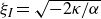 $\xi _{\textit{I}}=\sqrt {-2\kappa /\alpha }$
(Cates & Tjhung Reference Cates and Tjhung2018). The logarithmic term
$\xi _{\textit{I}}=\sqrt {-2\kappa /\alpha }$
(Cates & Tjhung Reference Cates and Tjhung2018). The logarithmic term
 $k_{\textit{B}}T c \ln (a^d c)$
captures the translational diffusion of the surfactant molecules. Similarly, the term
$k_{\textit{B}}T c \ln (a^d c)$
captures the translational diffusion of the surfactant molecules. Similarly, the term
 $dk_{\textit{B}}Tc |\boldsymbol{p}|^2/2$
accounts for the rotational diffusion. The term
$dk_{\textit{B}}Tc |\boldsymbol{p}|^2/2$
accounts for the rotational diffusion. The term
 $\chi \ell c \boldsymbol{p} \boldsymbol{\cdot }\boldsymbol{\nabla } \phi$
couples the surfactants to the fluid, causing them to be attracted and align perpendicular to the interface. In the absence of surfactant,
$\chi \ell c \boldsymbol{p} \boldsymbol{\cdot }\boldsymbol{\nabla } \phi$
couples the surfactants to the fluid, causing them to be attracted and align perpendicular to the interface. In the absence of surfactant,
 $c=0$
or
$c=0$
or
 $\chi =0$
, the bare surface tension of the water–oil interface is given by
$\chi =0$
, the bare surface tension of the water–oil interface is given by
 $\sigma _{\textit{I}}=\sqrt {-8\kappa \alpha ^3/(9\beta ^2)}$
. Equation (2.36) can alternatively be derived from direct calculation of the Shannon entropy and energy contributions to the Helmholtz free energy, as shown in Appendix A.
$\sigma _{\textit{I}}=\sqrt {-8\kappa \alpha ^3/(9\beta ^2)}$
. Equation (2.36) can alternatively be derived from direct calculation of the Shannon entropy and energy contributions to the Helmholtz free energy, as shown in Appendix A.
We emphasise that the coarse-grained mesoscopic free energy
 $F$
is distinct from the hybrid single-molecule–continuum-fluid free energy
$F$
is distinct from the hybrid single-molecule–continuum-fluid free energy
 $A$
in (2.8), which depends explicitly on the discrete particle position. In the absence of external flow,
$A$
in (2.8), which depends explicitly on the discrete particle position. In the absence of external flow,
 $\boldsymbol{v}_{\textit{ext}} = 0$
, one can show that the steady-state solution to the
$\boldsymbol{v}_{\textit{ext}} = 0$
, one can show that the steady-state solution to the
 $\boldsymbol{p}$
- and
$\boldsymbol{p}$
- and
 $c$
-dynamics in (2.34) and (2.35), respectively, is given by the minimum of the coarse-grained mesoscopic free energy:
$c$
-dynamics in (2.34) and (2.35), respectively, is given by the minimum of the coarse-grained mesoscopic free energy:
 \begin{align} \frac {\delta F}{\delta c} = 0 \quad \text{and}\quad \frac {\delta F}{\delta \boldsymbol{p}} = \boldsymbol{0}. \end{align}
This shows that the detailed balance property is preserved under coarse-graining: at the single-particle level, the equilibrium steady state is characterised by a Boltzmann distribution (see (2.29)), while at the coarse-grained level, it corresponds to the minimum of the mesoscopic free energy
 $F$
.
$F$
.
2.3. Coupling surfactant particle dynamics back to the fluid flow.
The results of the previous subsection neglect hydrodynamic effects due to the presence of the surfactants, as can be seen in the definition of
 $\boldsymbol{v}_{\textit{ext}}(\boldsymbol{r})$
in (2.19). To derive hydrodynamic flows from the surfactants, we again use the Rayleigh dissipation formalism. However, we now start with the coarse-grained free energy of (2.36) in our definition of the Rayleighian, so that (cf. (2.9))
$\boldsymbol{v}_{\textit{ext}}(\boldsymbol{r})$
in (2.19). To derive hydrodynamic flows from the surfactants, we again use the Rayleigh dissipation formalism. However, we now start with the coarse-grained free energy of (2.36) in our definition of the Rayleighian, so that (cf. (2.9))
 \begin{align} \mathcal{R}_{\textit{cg}}[\partial _t\phi ,\boldsymbol{v},\boldsymbol{v}_1,\partial _tc,\partial _t\boldsymbol{p}] = \varPhi _1[\boldsymbol{v}] + \varPhi _2[\boldsymbol{v}_1,\boldsymbol{v}_2] + \dot {F}, \end{align}
where
 \begin{align} \dot {F} = \int d^3 r\bigg (\frac {\delta F}{\delta \phi }\partial _t\phi +\frac {\delta F}{\delta c}\partial _tc +\frac {\delta F}{\delta \boldsymbol{p}}\partial _t\boldsymbol{p}\bigg ). \end{align}
Here,
 $\partial _t\phi$
,
$\partial _t\phi$
,
 $\partial _tc$
and
$\partial _tc$
and
 $\partial _t\boldsymbol{p}$
are defined in (2.17a
), (2.35) and (2.34). Within these equations, we replace the external field
$\partial _t\boldsymbol{p}$
are defined in (2.17a
), (2.35) and (2.34). Within these equations, we replace the external field
 $\boldsymbol{v}_{\textit{ext}}\to \boldsymbol{v}$
, where
$\boldsymbol{v}_{\textit{ext}}\to \boldsymbol{v}$
, where
 $\boldsymbol{v}(\boldsymbol{r},t)$
is now the total fluid velocity to be determined self-consistently, so
$\boldsymbol{v}(\boldsymbol{r},t)$
is now the total fluid velocity to be determined self-consistently, so
 \begin{align} \frac {\partial \phi (\boldsymbol{r},t)}{\partial t} + \boldsymbol{\nabla }\boldsymbol{\cdot }\left [\phi (\boldsymbol{r},t)\boldsymbol{v}(\boldsymbol{r},t) \right ] &= M{\nabla} ^2\frac {\delta F}{\delta \phi }, \\[-10pt] \nonumber \end{align}
 \begin{align} \frac {\partial c(\boldsymbol{r},t)}{\partial t} + \boldsymbol{\nabla }\boldsymbol{\cdot }\left [ c(\boldsymbol{r},t)\boldsymbol{v}(\boldsymbol{r},t) \right ] &= \boldsymbol{\nabla }\boldsymbol{\cdot }\left [ \frac {1}{\gamma _t}c(\boldsymbol{r},t)\boldsymbol{\nabla }\left (\frac {\delta F}{\delta c}\right ) \right ], \\[-10pt] \nonumber \end{align}
 \begin{align} \frac {\partial \boldsymbol{p}(\boldsymbol{r},t)}{\partial t} + \boldsymbol{v}(\boldsymbol{r},t)\boldsymbol{\cdot }\boldsymbol{\nabla }\boldsymbol{p}(\boldsymbol{r},t) &= -\frac {d-1}{d\gamma _rc(\boldsymbol{r},t)}\frac {\delta F}{\delta \boldsymbol{p}} +\left [ \! \frac {Bd}{d+2}\boldsymbol{D}(\boldsymbol{r},t) - \boldsymbol{\varOmega }(\boldsymbol{r},t) \! \right ] \boldsymbol{\cdot }\boldsymbol{p}(\boldsymbol{r},t), \end{align}
where
 $F$
is given in (2.36). Inserting these equations into the free energy dissipation and taking functional derivatives with respect to
$F$
is given in (2.36). Inserting these equations into the free energy dissipation and taking functional derivatives with respect to
 $\boldsymbol{v}$
and
$\boldsymbol{v}$
and
 $\boldsymbol{v}_1$
(with
$\boldsymbol{v}_1$
(with
 $\boldsymbol{v}=(1+\phi )\boldsymbol{v}_1/2+(1-\phi )\boldsymbol{v}_2/2$
), we find the Stokes equation
$\boldsymbol{v}=(1+\phi )\boldsymbol{v}_1/2+(1-\phi )\boldsymbol{v}_2/2$
), we find the Stokes equation
 \begin{eqnarray} && 0= \eta {\nabla} ^2\boldsymbol{v} - \boldsymbol{\nabla }P -(1+\phi )\boldsymbol{\nabla }\frac {\delta F}{\delta \phi } - c\boldsymbol{\nabla }\frac {\delta F}{\delta c} - \boldsymbol{p}\boldsymbol{\cdot }\left (\boldsymbol{\nabla }\frac {\delta F}{\delta \boldsymbol{p}}\right )^T \nonumber\\ && \qquad +\, \frac {Bd}{2(d+2)}\boldsymbol{\nabla }\boldsymbol{\cdot }\left ( \boldsymbol{p}\frac {\delta F}{\delta \boldsymbol{p}} + \frac {\delta F}{\delta \boldsymbol{p}}\boldsymbol{p} \right ) -\frac {1}{2}\boldsymbol{\nabla }\boldsymbol{\cdot }\left (\boldsymbol{p}\frac {\delta F}{\delta \boldsymbol{p}} - \frac {\delta F}{\delta \boldsymbol{p}}\boldsymbol{p} \right ) \end{eqnarray}
where
 $P$
is the pressure enforcing incompressibility
$P$
is the pressure enforcing incompressibility
 $\boldsymbol{\nabla }\boldsymbol{\cdot }\boldsymbol{v}=0$
. Note that the
$\boldsymbol{\nabla }\boldsymbol{\cdot }\boldsymbol{v}=0$
. Note that the
 $-\boldsymbol{\nabla }\delta F/\delta \phi$
term in (2.41) can be absorbed into the pressure term
$-\boldsymbol{\nabla }\delta F/\delta \phi$
term in (2.41) can be absorbed into the pressure term
 $-\boldsymbol{\nabla }P$
. Equations (2.40) and (2.41) completely describe the dynamics of the surfactant in a binary fluid system for the case of non-interacting surfactant molecules (they are only interacting through the fluid velocity). The mathematical structure of the stress-like tensor in the Stokes equation (2.41) is consistent with the Cauchy stress previously obtained for polar liquid crystals (Cates & Tjhung Reference Cates and Tjhung2018; Markovich, Tjhung & Cates (Reference Markovich, Tjhung and Cates2019).
$-\boldsymbol{\nabla }P$
. Equations (2.40) and (2.41) completely describe the dynamics of the surfactant in a binary fluid system for the case of non-interacting surfactant molecules (they are only interacting through the fluid velocity). The mathematical structure of the stress-like tensor in the Stokes equation (2.41) is consistent with the Cauchy stress previously obtained for polar liquid crystals (Cates & Tjhung Reference Cates and Tjhung2018; Markovich, Tjhung & Cates (Reference Markovich, Tjhung and Cates2019).
In the absence of external driving, minimising the Rayleighian dissipation functional yields the equilibrium equations of motion for the system. When a flow field is imposed, e.g. a shear flow, the Rayleighian simply acquires an additional contribution associated with the externally driven fluid flow. Minimising this modified functional produces the full equations governing both the transient dynamics and the resulting non-equilibrium steady state. Thus, the Rayleighian formalism provides a unified description of equilibrium and driven non-equilibrium behaviour, without the need for separate modelling assumptions.
3. Results and discussion
To demonstrate the validity and reliability of our model, we present three case studies. The first examines a planar interface under the assumption of weak coupling, where we show that the system equations can be solved analytically via perturbation theory to any desired order. Numerical results are also provided, showing excellent agreement with our analytical solutions. The second case study extends this system by using the perturbative solutions to calculate the surface tension of a surfactant-loaded interface, where the presence of surfactants leads to a decrease in surface tension. Finally, we demonstrate how the inclusion of surfactants may suppress the coalescence of oil droplets.
3.1. Non-dimensionalisation and numerical method of solution
All of the following simulation results are presented in dimensionless units. Without loss of generality, we set
 $\alpha = -\beta$
in the free energy expression (2.36), so that the bulk free energy favours phase separation into
$\alpha = -\beta$
in the free energy expression (2.36), so that the bulk free energy favours phase separation into
 $\phi = \pm 1$
. We choose the interfacial width of the pure binary fluid,
$\phi = \pm 1$
. We choose the interfacial width of the pure binary fluid,
 $\xi _{\textit{I}} = \sqrt {2\kappa /\beta }$
as the unit of length,
$\xi _{\textit{I}} = \sqrt {2\kappa /\beta }$
as the unit of length,
 $\tau$
as the unit of time and
$\tau$
as the unit of time and
 $k_{\textit{B}}T$
as the unit of energy. We also introduce a small (dimensionless) parameter
$k_{\textit{B}}T$
as the unit of energy. We also introduce a small (dimensionless) parameter
 $\varepsilon = \chi \ell / ( \xi _{\textit{I}} k_{\textit{B}}T )$
to represent the weak coupling between the fluid and surfactants. Physically,
$\varepsilon = \chi \ell / ( \xi _{\textit{I}} k_{\textit{B}}T )$
to represent the weak coupling between the fluid and surfactants. Physically,
 $\varepsilon$
characterises the interaction strength between the surfactant molecules and the binary fluid interface (relative to
$\varepsilon$
characterises the interaction strength between the surfactant molecules and the binary fluid interface (relative to
 $k_{\textit{B}}T$
). For simplicity, we retain the same notation for the non-dimensionalised constants and variables as in the dimensional forms. More details can be found in Appendix C. The dimensionless Helmholtz free energy is then given by
$k_{\textit{B}}T$
). For simplicity, we retain the same notation for the non-dimensionalised constants and variables as in the dimensional forms. More details can be found in Appendix C. The dimensionless Helmholtz free energy is then given by
 \begin{align} F[\phi ,c,\boldsymbol{p}] = \int \left \{ -\frac {\beta }{2}\phi ^2 + \frac {\beta }{4} \phi ^4 + \frac {\beta }{4}|\boldsymbol{\nabla }\phi |^2 + c\ln (c) +\frac {d}{2}c|\boldsymbol{p}|^2 + \varepsilon c \kern-1.5pt \boldsymbol{p}\boldsymbol{\cdot }\boldsymbol{\nabla }\phi \right \} d^dr, \end{align}
and the resulting system of coupled partial differential equations governing the dynamics of the binary fluid volume fraction, surfactant concentration, average orientation field and fluid velocity can be expressed as
 \begin{align} \frac {\partial \phi }{\partial t}+(\boldsymbol{v}\boldsymbol{\cdot }\boldsymbol{\nabla }) \phi = M{\nabla} ^2\left (\frac {\delta F}{\delta \phi }\right ) & = M {\nabla} ^2 \left [-\beta \phi + \beta \phi ^3 - \frac {\beta }{2}{\nabla} ^2\phi - \varepsilon \boldsymbol{\nabla }\boldsymbol{\cdot }(c \kern-1.5pt \boldsymbol{p}) \right ], \end{align}
 \begin{align} \frac {\partial c}{\partial t}+(\boldsymbol{v}\boldsymbol{\cdot }\boldsymbol{\nabla })c = \boldsymbol{\nabla }\boldsymbol{\cdot }\left [\frac {c}{\gamma _t}\boldsymbol{\nabla } \left (\frac {\delta F}{\delta c}\right ) \right ] &= \frac {1}{\gamma _t}{\nabla} ^2c + \frac {1}{\gamma _t} \boldsymbol{\nabla } \boldsymbol{\cdot }\left [ c\boldsymbol{\nabla }\left (\frac {d}{2}|\boldsymbol{p}|^2+\varepsilon \boldsymbol{p}\boldsymbol{\cdot }\boldsymbol{\nabla } \phi \right )\right ], \end{align}
 \begin{align} \frac {\partial \boldsymbol{p}}{\partial t}+(\boldsymbol{v} \boldsymbol{\cdot }\boldsymbol{\nabla })\boldsymbol{p} + \boldsymbol{\varOmega }\boldsymbol{\cdot }\boldsymbol{p} - \frac {B{\rm d}}{d+2}\boldsymbol{D}\boldsymbol{\cdot }\boldsymbol{p} &= -\frac {d-1}{d\gamma _r c} \left (\frac {\delta F}{\delta \boldsymbol{p}}\right ) = -\frac {d-1}{d\gamma _r}({\rm d}\kern-1pt \boldsymbol{p} + \varepsilon \boldsymbol{\nabla }\phi ), \\[-10pt] \nonumber \end{align}
 \begin{align} 0 &=-\boldsymbol{\nabla }P + \eta {\nabla} ^2\boldsymbol{v}+\boldsymbol{f} + \boldsymbol{\nabla }\boldsymbol{\cdot }\boldsymbol{\sigma }, \\[-10pt] \nonumber \end{align}
 \begin{align} 0 &= \boldsymbol{\nabla } \boldsymbol{\cdot }\boldsymbol{v}, \end{align}
where we have defined the body force
 \begin{align} \boldsymbol{f} \equiv -\phi \boldsymbol{\nabla }\frac {\delta F}{\delta \phi } -c\boldsymbol{\nabla }\frac {\delta F}{\delta c} -\boldsymbol{p}\boldsymbol{\cdot }\bigg (\boldsymbol{\nabla }\frac {\delta F}{\delta \boldsymbol{p}}\bigg )^T \end{align}
and the stress-like tensor
 \begin{align} \boldsymbol{\sigma } \equiv \frac {Bd}{2(d+2)} \left (\boldsymbol{p}\frac {\delta F}{\delta \boldsymbol{p}} + \frac {\delta F}{\delta \boldsymbol{p}}\boldsymbol{p}\right ) -\frac {1}{2} \left (\boldsymbol{p}\frac {\delta F}{\delta \boldsymbol{p}} -\frac {\delta F}{\delta \boldsymbol{p}}\boldsymbol{p}\right ). \end{align}
In the dimensionless unit, the bare surface tension is then given by
 $\sigma _{\textit{I}}=2\beta /3$
. For the remainder of this paper, we consider the two-dimensional case (
$\sigma _{\textit{I}}=2\beta /3$
. For the remainder of this paper, we consider the two-dimensional case (
 $d=2$
) only.
$d=2$
) only.
In the following, we briefly outline the general numerical scheme employed in our study, based on the dimensionless (3.2). We consider a two-dimensional domain of size
 $L_x$
in the
$L_x$
in the
 $x$
-direction and
$x$
-direction and
 $L_y$
in the
$L_y$
in the
 $y$
-direction. We employ a simple finite difference method with Euler time-stepping to simulate the variables
$y$
-direction. We employ a simple finite difference method with Euler time-stepping to simulate the variables
 $\phi (\boldsymbol{r},t)$
,
$\phi (\boldsymbol{r},t)$
,
 $c(\boldsymbol{r},t)$
and
$c(\boldsymbol{r},t)$
and
 $\boldsymbol{p}(\boldsymbol{r},t)$
. This is implemented using the Python library NumPy (Harris et al. Reference Harris2020). Central differences are used for both first- and second-order derivatives. We assume periodic boundary conditions at
$\boldsymbol{p}(\boldsymbol{r},t)$
. This is implemented using the Python library NumPy (Harris et al. Reference Harris2020). Central differences are used for both first- and second-order derivatives. We assume periodic boundary conditions at
 $y=0$
and
$y=0$
and
 $y=L_y$
. Boundary conditions at
$y=L_y$
. Boundary conditions at
 $x=0$
and
$x=0$
and
 $x=L_x$
can either be no-flux or periodic. No-flux conditions are derived to conserve
$x=L_x$
can either be no-flux or periodic. No-flux conditions are derived to conserve
 $\phi (\boldsymbol{r},t)$
and
$\phi (\boldsymbol{r},t)$
and
 $c(\boldsymbol{r},t)$
, resulting in either Neumann or reflective boundary conditions, as detailed in Appendix D. Unless otherwise specified, the values for all parameters used in the simulations are provided in Appendix C.
$c(\boldsymbol{r},t)$
, resulting in either Neumann or reflective boundary conditions, as detailed in Appendix D. Unless otherwise specified, the values for all parameters used in the simulations are provided in Appendix C.
At each time step, the fluid velocity
 $\boldsymbol{v}$
is calculated using a pseudospectral method as outlined by Hardy et al. (Reference Hardy, Daddi-Moussa-Ider and Tjhung2024). By transforming the Stokes equation (3.2d
) into Fourier space (where Fourier-space variables are denoted with a tilde), we obtain the expression used to calculate the velocity at each time step:
$\boldsymbol{v}$
is calculated using a pseudospectral method as outlined by Hardy et al. (Reference Hardy, Daddi-Moussa-Ider and Tjhung2024). By transforming the Stokes equation (3.2d
) into Fourier space (where Fourier-space variables are denoted with a tilde), we obtain the expression used to calculate the velocity at each time step:
 \begin{align} \widetilde {\boldsymbol{v}}_{\boldsymbol{k}} = \frac {1}{\eta k^2} \left [\widetilde {\boldsymbol{f}}_{\boldsymbol{k}} - \left ( \widetilde {\boldsymbol{f}}_{\boldsymbol{k}}\boldsymbol{\cdot }\hat {\boldsymbol{k}} \right ) \hat {\boldsymbol{k}} \right ], \end{align}
where
 $\boldsymbol{k}$
is the wavevector,
$\boldsymbol{k}$
is the wavevector,
 $k = |\boldsymbol{k}|$
is the corresponding wavenumber and
$k = |\boldsymbol{k}|$
is the corresponding wavenumber and
 $\hat {\boldsymbol{k}} = \boldsymbol{k}/k$
is the unit wavevector. The forcing term
$\hat {\boldsymbol{k}} = \boldsymbol{k}/k$
is the unit wavevector. The forcing term
 $\widetilde {\boldsymbol{f}}_{\boldsymbol{k}}$
encompasses all terms from
$\widetilde {\boldsymbol{f}}_{\boldsymbol{k}}$
encompasses all terms from
 $\boldsymbol{f}$
and
$\boldsymbol{f}$
and
 $\boldsymbol{\nabla } \boldsymbol{\cdot }\boldsymbol{\sigma }$
. The Fourier-space pressure is
$\boldsymbol{\nabla } \boldsymbol{\cdot }\boldsymbol{\sigma }$
. The Fourier-space pressure is
 \begin{align} \widetilde {P}_{\boldsymbol{k}} = -\frac {i}{k} \widetilde {\boldsymbol{f}}_{\boldsymbol{k}}\boldsymbol{\cdot }\hat {\boldsymbol{k}}. \end{align}
As with
 $\phi$
,
$\phi$
,
 $c$
and
$c$
and
 $\boldsymbol{p}$
, we impose periodic boundary conditions on
$\boldsymbol{p}$
, we impose periodic boundary conditions on
 $\boldsymbol{v}$
at
$\boldsymbol{v}$
at
 $y=0$
and
$y=0$
and
 $y=L_y$
. Along the
$y=L_y$
. Along the
 $x$
-direction, the fluid velocity
$x$
-direction, the fluid velocity
 $\boldsymbol{v}$
can satisfy either no-slip or periodic boundary conditions. In the case of no-slip boundary conditions at
$\boldsymbol{v}$
can satisfy either no-slip or periodic boundary conditions. In the case of no-slip boundary conditions at
 $x=0$
and
$x=0$
and
 $x=L_x$
, combined with periodic boundary conditions at
$x=L_x$
, combined with periodic boundary conditions at
 $y=0$
and
$y=0$
and
 $y=L_y$
, it is convenient to use a sine transform in
$y=L_y$
, it is convenient to use a sine transform in
 $x$
and a standard Fourier transform in
$x$
and a standard Fourier transform in
 $y$
, i.e.
$y$
, i.e.
 \begin{align} \boldsymbol{v}(\boldsymbol{r}) = \sqrt {\frac {2}{L_xL_y}} \sum _{n,m} \widetilde {\boldsymbol{v}}_{\boldsymbol{k}} \sin \left (\frac {n\pi x }{L_x}\right ) e^{i\frac {2\pi my}{L_y}} , \end{align}
where
 $n=1,2,3,\ldots$
and
$n=1,2,3,\ldots$
and
 $m\in \mathbb{Z}$
. The corresponding discrete wavevector
$m\in \mathbb{Z}$
. The corresponding discrete wavevector
 $\boldsymbol{k}=(k_x,k_y)^T$
are given by
$\boldsymbol{k}=(k_x,k_y)^T$
are given by
 $k_x=\pi n/L_x$
and
$k_x=\pi n/L_x$
and
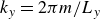 $k_y=2\pi m/L_y$
, see https://github.com/AlexHardy0/Surfactants for detailed implementation.
$k_y=2\pi m/L_y$
, see https://github.com/AlexHardy0/Surfactants for detailed implementation.
We validated our model by simulating a pure binary fluid and obtaining the classical solution for a clean binary fluid (Cates & Tjhung Reference Cates and Tjhung2018). The pseudospectral scheme used for velocity was also validated through the Poiseuille flow example, where it perfectly matched the analytical solutions.
3.2. Planar interface
Our first case study involves a flat, vertical water–oil interface at
 $x=0$
, as shown in figure 3(b). Over time, surfactants adsorb onto the interface, resulting in a peak in concentration
$x=0$
, as shown in figure 3(b). Over time, surfactants adsorb onto the interface, resulting in a peak in concentration
 $c(\boldsymbol{r},t)$
, although some surfactant concentration remains in the bulk phases. Additionally, the surfactant molecules align perpendicular to the interface, with the ‘head’ in the water phase and the ‘tail’ in the oil phase, as indicated by the non-zero
$c(\boldsymbol{r},t)$
, although some surfactant concentration remains in the bulk phases. Additionally, the surfactant molecules align perpendicular to the interface, with the ‘head’ in the water phase and the ‘tail’ in the oil phase, as indicated by the non-zero
 $x$
-component of
$x$
-component of
 $\boldsymbol{p}(\boldsymbol{r},t)$
. When
$\boldsymbol{p}(\boldsymbol{r},t)$
. When
 $|\boldsymbol{p}| \gt 0$
, the molecules are aligned, as opposed to being randomly arranged when
$|\boldsymbol{p}| \gt 0$
, the molecules are aligned, as opposed to being randomly arranged when
 $\boldsymbol{p} \approx \boldsymbol{0}$
. At equilibrium, the fluid velocity falls to zero and the system reaches a static configuration. Assuming
$\boldsymbol{p} \approx \boldsymbol{0}$
. At equilibrium, the fluid velocity falls to zero and the system reaches a static configuration. Assuming
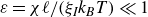 $\varepsilon = \chi \ell / (\xi _{\textit{I}} k_{\textit{B}}T ) \ll 1$
, we can solve the steady-state solution perturbatively.
$\varepsilon = \chi \ell / (\xi _{\textit{I}} k_{\textit{B}}T ) \ll 1$
, we can solve the steady-state solution perturbatively.
We now solve the system of nonlinear ordinary differential equation (3.2) (with
 $d=2$
) using a regular perturbation approach. Due to translational symmetry in the
$d=2$
) using a regular perturbation approach. Due to translational symmetry in the
 $y$
-direction, the solutions depend only on the
$y$
-direction, the solutions depend only on the
 $x$
-direction. At steady-state equilibrium, the system equations then simplify to
$x$
-direction. At steady-state equilibrium, the system equations then simplify to
 \begin{align} \beta \left ( \phi - \phi ^3 + \frac {1}{2} \, \phi '' \right ) + \varepsilon \, (cp_x)' &= 0 , \end{align}
 \begin{align} c' + c (p_x^2)' + \varepsilon c (p_x \phi ')' &= 0 , \end{align}
 \begin{align} 2p_x + \varepsilon \phi ' &= 0 , \end{align}
where
 $p_x$
is the
$p_x$
is the
 $x$
-component of the field
$x$
-component of the field
 $\boldsymbol{p}(\boldsymbol{r},t)$
. Here, primes indicate differentiation with respect to
$\boldsymbol{p}(\boldsymbol{r},t)$
. Here, primes indicate differentiation with respect to
 $x$
. It follows from (3.8c
) that
$x$
. It follows from (3.8c
) that
 \begin{align} p_x = -\frac {1}{2} \, \varepsilon \phi ' \, . \end{align}
Thus, we only need to find the solution for the fields
 $ \phi$
and
$ \phi$
and
 $ c$
. Substituting (3.9) into (3.8a
) and (3.8b
), we obtain
$ c$
. Substituting (3.9) into (3.8a
) and (3.8b
), we obtain
 \begin{align} \beta \big ( 2\phi - 2\phi ^3 + \phi '' \big ) - \varepsilon ^2 \, (c\phi ')' &= 0 , \end{align}
 \begin{align} 2c' + \varepsilon ^2 c \phi ' \phi '' -\varepsilon ^2 c ( {\phi '}^2)' &= 0 . \end{align}
Equations (3.10) are highly nonlinear, making an analytical solution challenging. To address this, we seek an approximate solution using the perturbation method, expressing the solution as
 \begin{align} \phi (x) &= \phi _0(x) + \phi _2(x) \, \varepsilon ^2 + \phi _4(x) \, \varepsilon ^4 + \mathcal{O} (\varepsilon ^6) , \end{align}
 \begin{align} c(x) &= c_0(x) + c_2(x) \, \varepsilon ^2 + c_4(x) \, \varepsilon ^4 + \mathcal{O} (\varepsilon ^6). \\[9pt] \nonumber \end{align}
Due to parity considerations, we expect the odd powers in the series expansions of
 $ \phi$
and
$ \phi$
and
 $ c$
to vanish. Inserting the perturbation expansion into (3.10) yields the zeroth-order problem as
$ c$
to vanish. Inserting the perturbation expansion into (3.10) yields the zeroth-order problem as
 \begin{align} \phi _0'' + 2\phi _0 - 2\phi _0^3 &= 0 , \end{align}
 \begin{align} c_0' &= 0 , \end{align}
the solution of which is given by
 \begin{align} \phi _0(x) &= \tanh x , \end{align}
 \begin{align} c_0(x) &= C_0 = \text{const.} , \end{align}
where
 $\tanh$
represents the hyperbolic tangent function and
$\tanh$
represents the hyperbolic tangent function and
 $C_0$
is some constant. To simplify the equations, we introduce the abbreviation
$C_0$
is some constant. To simplify the equations, we introduce the abbreviation
 $ \lambda = C_0/\beta$
as well as the function
$ \lambda = C_0/\beta$
as well as the function
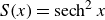 $ S(x) = \operatorname {sech}^2 x$
. The order
$ S(x) = \operatorname {sech}^2 x$
. The order
 $ \varepsilon ^2$
equations are obtained as
$ \varepsilon ^2$
equations are obtained as
 \begin{align} \beta \phi _2'' + 2\beta \big ( 1-3\phi _0^2 \big ) \phi _2 - C_0 \phi _0''&= 0 , \end{align}
 \begin{align} 2 c_2' - C_0 \phi _0' \phi _0'' &= 0 . \end{align}
The solution to this is given by
 \begin{align} \phi _2(x) &= \frac {1}{2} \, \lambda x S(x) , \end{align}
 \begin{align} c_2(x) &= \frac {1}{4} \, C_0 S(x)^2 . \end{align}
The equations at order
 $ \varepsilon ^4$
are given by
$ \varepsilon ^4$
are given by
 \begin{align} \beta \phi _4'' + 2\beta ( 1- 3\phi _0^2 ) \phi _4 &= c_2\phi _0''+C_0\phi _2'' + c_2'\phi _0' + 6\beta \phi _0\phi _2^2 , \end{align}
 \begin{align} 2c_4' &= C_0 \phi _0' \phi _2'' + \left ( C_0 \phi _2'+c_2 \phi _0' \right ) \phi _0'' . \end{align}
The solution to this is given by
 \begin{align} \phi _4(x) &= \frac {1}{16} \, \lambda S(x) \big ( 6\lambda x + \big ( 2 -4\lambda x^2 + S(x) \big )\tanh x \big ) , \end{align}
 \begin{align} c_4(x) &= \frac {1}{32} \, C_0 S(x)^2 \big ( 8\lambda ( 1-2 x \tanh x) + S(x)^2 \big ) . \end{align}
In theory, we could extend beyond the current order and determine higher-order terms in the perturbation series. However, due to technical limitations and the complexity of the resulting expressions, we stop at the current order. We expect the series to provide an accurate approximation of the solution, provided that
 $ \varepsilon \ll 1$
.
$ \varepsilon \ll 1$
.
From (3.9), it follows that the polarisation can be expressed as an odd power series in
 $ \varepsilon$
, given by
$ \varepsilon$
, given by
 \begin{align} p_x(x) = p_{x1}(x) \varepsilon + p_{x3}(x) \varepsilon ^3 + p_{x5}(x) \varepsilon ^5 + \mathcal{O} ( \varepsilon ^7 ). \end{align}
We find after calculation that
 \begin{align} p_{x1}(x) &= -\frac {1}{2} \, S(x) , \end{align}
 \begin{align} p_{x3}(x) &= \frac {1}{4} \, \lambda S(x) \left ( 2x\tanh x-1\right ) , \end{align}
 \begin{align} p_{x5}(x) &= \frac {1}{32} \, \lambda S(x) \big ( 4-6\lambda -8\lambda x^2 +20\lambda x \tanh x + ( 12\lambda x^2-2) S(x) -5 S(x)^2 \big ) . \end{align}
For comparison, we also simulate the same scenario using the numerical scheme described in § 3.1. We use a two-dimensional rectangular computational domain sized
 $L_x=64$
and
$L_x=64$
and
 $L_y=4$
with a spatial resolution of
$L_y=4$
with a spatial resolution of
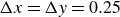 $\Delta x=\Delta y=0.25$
and temporal resolution of
$\Delta x=\Delta y=0.25$
and temporal resolution of
 $\Delta t=0.0001$
. We use a uniform initial condition for
$\Delta t=0.0001$
. We use a uniform initial condition for
 $c(\boldsymbol{r},t)$
, with initial concentration value
$c(\boldsymbol{r},t)$
, with initial concentration value
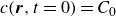 $c(\boldsymbol{r},t = 0) = C_0$
. Physically,
$c(\boldsymbol{r},t = 0) = C_0$
. Physically,
 $C_0$
represents the average surfactant concentration, which is conserved throughout. Volume fraction field
$C_0$
represents the average surfactant concentration, which is conserved throughout. Volume fraction field
 $\phi (\boldsymbol{r},t)$
is initialised as two halves, with
$\phi (\boldsymbol{r},t)$
is initialised as two halves, with
 $\phi (x \lt 0) = -1.0$
(water) and
$\phi (x \lt 0) = -1.0$
(water) and
 $\phi (x \gt 0) = 1.0$
(oil). Each phase has a magnitude of
$\phi (x \gt 0) = 1.0$
(oil). Each phase has a magnitude of
 $1$
as that is the solution of the double well potential in the free energy density. All other fields are initialised as zero everywhere. We have periodic boundary conditions at
$1$
as that is the solution of the double well potential in the free energy density. All other fields are initialised as zero everywhere. We have periodic boundary conditions at
 $y=0$
and
$y=0$
and
 $y=L_y$
, and no-slip/no-flux boundary conditions at
$y=L_y$
, and no-slip/no-flux boundary conditions at
 $x=-L_x/2$
and
$x=-L_x/2$
and
 $x=L_x/2$
. This is to ensure that only one water–oil interface is created. We choose to vary two parameters,
$x=L_x/2$
. This is to ensure that only one water–oil interface is created. We choose to vary two parameters,
 $\varepsilon$
and the average surfactant concentration
$\varepsilon$
and the average surfactant concentration
 $C_0$
. Three simulations were run in total, with parameters:
$C_0$
. Three simulations were run in total, with parameters:
 $\varepsilon = 0.0$
and
$\varepsilon = 0.0$
and
 $C_0 = 0$
(clean system), one with
$C_0 = 0$
(clean system), one with
 $\varepsilon = 0.3$
and
$\varepsilon = 0.3$
and
 $C_0 = 1.6$
, and another with
$C_0 = 1.6$
, and another with
 $\varepsilon = 0.5$
and
$\varepsilon = 0.5$
and
 $C_0 = 3.1$
.
$C_0 = 3.1$
.
(a) A graph showing the analytical (line) and numerical (symbols) solutions for the fluid field
 $\phi (x)$
with the leading order
$\phi (x)$
with the leading order
 $\phi _0(x) = \tanh {x}$
removed, at equilibrium for a variety of
$\phi _0(x) = \tanh {x}$
removed, at equilibrium for a variety of
 $\varepsilon$
and
$\varepsilon$
and
 $C_0$
values. (b) A graph showing the analytical (line) and numerical (symbols) solutions for concentration
$C_0$
values. (b) A graph showing the analytical (line) and numerical (symbols) solutions for concentration
 $c(x)$
with the leading order
$c(x)$
with the leading order
 $c_0(x)=C_0$
removed, at equilibrium for a range of
$c_0(x)=C_0$
removed, at equilibrium for a range of
 $\varepsilon$
and
$\varepsilon$
and
 $C_0$
values. (c) A graph showing the analytical (line) and numerical (symbols) solutions for the polarisation field
$C_0$
values. (c) A graph showing the analytical (line) and numerical (symbols) solutions for the polarisation field
 $p_x(x,t)$
, at equilibrium for a range of
$p_x(x,t)$
, at equilibrium for a range of
 $\varepsilon$
and
$\varepsilon$
and
 $C_0$
values. Parameters used:
$C_0$
values. Parameters used:
 $\beta =2.0$
,
$\beta =2.0$
,
 $B=0.5$
,
$B=0.5$
,
 $M=3$
,
$M=3$
,
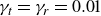 $\gamma _t=\gamma _r=0.01$
.
$\gamma _t=\gamma _r=0.01$
.
Figure 2 show the steady-state profiles
 $\phi (x,t\rightarrow \infty )$
,
$\phi (x,t\rightarrow \infty )$
,
 $c(x,t\rightarrow \infty )$
and
$c(x,t\rightarrow \infty )$
and
 $p_x(x,t\rightarrow \infty )$
, demonstrating excellent agreement with the perturbation theory. The deviations in
$p_x(x,t\rightarrow \infty )$
, demonstrating excellent agreement with the perturbation theory. The deviations in
 $\phi (\boldsymbol{r},t)$
remain small relative to the bulk values (
$\phi (\boldsymbol{r},t)$
remain small relative to the bulk values (
 $\pm 1$
), indicating that the fluid is only weakly perturbed, consistent with earlier studies, which also assume weak coupling between the fluid density and surfactant concentrations (van der Sman & van der Graaf Reference van der Sman and van der Graaf2006; Liu & Zhang Reference Liu and Zhang2010), although these studies did not incorporate an explicit polarisation field
$\pm 1$
), indicating that the fluid is only weakly perturbed, consistent with earlier studies, which also assume weak coupling between the fluid density and surfactant concentrations (van der Sman & van der Graaf Reference van der Sman and van der Graaf2006; Liu & Zhang Reference Liu and Zhang2010), although these studies did not incorporate an explicit polarisation field
 $\boldsymbol{p}(\boldsymbol{r},t)$
. As expected, the magnitude of deviations increases with both the coupling strength
$\boldsymbol{p}(\boldsymbol{r},t)$
. As expected, the magnitude of deviations increases with both the coupling strength
 $\varepsilon$
and the mean surfactant concentration
$\varepsilon$
and the mean surfactant concentration
 $C_0$
. The concentration profile
$C_0$
. The concentration profile
 $c(\boldsymbol{r},t\rightarrow \infty )$
exhibits a peak localised around the interface, with enhancements of the order of
$c(\boldsymbol{r},t\rightarrow \infty )$
exhibits a peak localised around the interface, with enhancements of the order of
 $0.2$
, comparable to values reported in prior numerical studies (van der Sman & van der Graaf Reference van der Sman and van der Graaf2006; Liu & Zhang Reference Liu and Zhang2010; Zong et al. Reference Zong, Zhang, Liang, Wang and Xu2020), again in the absence of a polarisation field.
$0.2$
, comparable to values reported in prior numerical studies (van der Sman & van der Graaf Reference van der Sman and van der Graaf2006; Liu & Zhang Reference Liu and Zhang2010; Zong et al. Reference Zong, Zhang, Liang, Wang and Xu2020), again in the absence of a polarisation field.
As
 $\varepsilon$
increases, more surfactant molecules are adsorbed at the interface due to the stronger attraction, leading to a higher peak in the surfactant concentration. The absorbed molecules exhibit alignment, as indicated by the peak in
$\varepsilon$
increases, more surfactant molecules are adsorbed at the interface due to the stronger attraction, leading to a higher peak in the surfactant concentration. The absorbed molecules exhibit alignment, as indicated by the peak in
 $p_x(x,t\rightarrow \infty )$
near the interface. Since the leading-order contribution to
$p_x(x,t\rightarrow \infty )$
near the interface. Since the leading-order contribution to
 $p_x(x,t\rightarrow \infty )$
is zero, this peak arises entirely from perturbative corrections. At equilibrium, molecular orientation at the interface exhibits minimal noise, with the
$p_x(x,t\rightarrow \infty )$
is zero, this peak arises entirely from perturbative corrections. At equilibrium, molecular orientation at the interface exhibits minimal noise, with the
 $y$
-component of
$y$
-component of
 $\boldsymbol{p}(\boldsymbol{r},t\rightarrow \infty )$
remaining negligible. We observe little dependence of the alignment strength on
$\boldsymbol{p}(\boldsymbol{r},t\rightarrow \infty )$
remaining negligible. We observe little dependence of the alignment strength on
 $C_0$
, indicating that increasing the number of adsorbed surfactant molecules does not significantly affect their collective orientation. Instead, alignment is more strongly governed by the coupling strength
$C_0$
, indicating that increasing the number of adsorbed surfactant molecules does not significantly affect their collective orientation. Instead, alignment is more strongly governed by the coupling strength
 $\varepsilon$
, which determines the effective attraction to the interface. Overall, the simulations show excellent agreement with the perturbative theory and are consistent with established understanding of surfactant behaviour at fluid interfaces at microscopic level.
$\varepsilon$
, which determines the effective attraction to the interface. Overall, the simulations show excellent agreement with the perturbative theory and are consistent with established understanding of surfactant behaviour at fluid interfaces at microscopic level.
(a) Effective surface tension divided by the bare surface tension
 $\sigma _{\textit{eff}}/\sigma {\text{I}}$
as a function of bulk surfactant concentration
$\sigma _{\textit{eff}}/\sigma {\text{I}}$
as a function of bulk surfactant concentration
 $C_0$
for different values of coupling strength
$C_0$
for different values of coupling strength
 $\varepsilon$
and fixed
$\varepsilon$
and fixed
 $\beta =1$
. Dashed lines indicate the leading-order prediction from the Gibbs isotherm. (b) Equilibrium configuration of a planar interface located at
$\beta =1$
. Dashed lines indicate the leading-order prediction from the Gibbs isotherm. (b) Equilibrium configuration of a planar interface located at
 $x=0$
. Black arrows show the polarisation field
$x=0$
. Black arrows show the polarisation field
 $\boldsymbol{p}$
which aligns perpendicular to the interface. (c) Under strong shear flow, the polarisation
$\boldsymbol{p}$
which aligns perpendicular to the interface. (c) Under strong shear flow, the polarisation
 $\boldsymbol{p}$
field becomes tilted and is no longer perpendicular to the interface. Blue arrows indicate the fluid velocity
$\boldsymbol{p}$
field becomes tilted and is no longer perpendicular to the interface. Blue arrows indicate the fluid velocity
 $\boldsymbol{v}$
. Parameters used:
$\boldsymbol{v}$
. Parameters used:
 $\beta =1.0$
,
$\beta =1.0$
,
 $B=1.0$
,
$B=1.0$
,
 $M=1.0$
,
$M=1.0$
,
 $\gamma _t=\gamma _r=0.1$
,
$\gamma _t=\gamma _r=0.1$
,
 $\eta =1.0$
and
$\eta =1.0$
and
 $\varepsilon =0.5$
.
$\varepsilon =0.5$
.
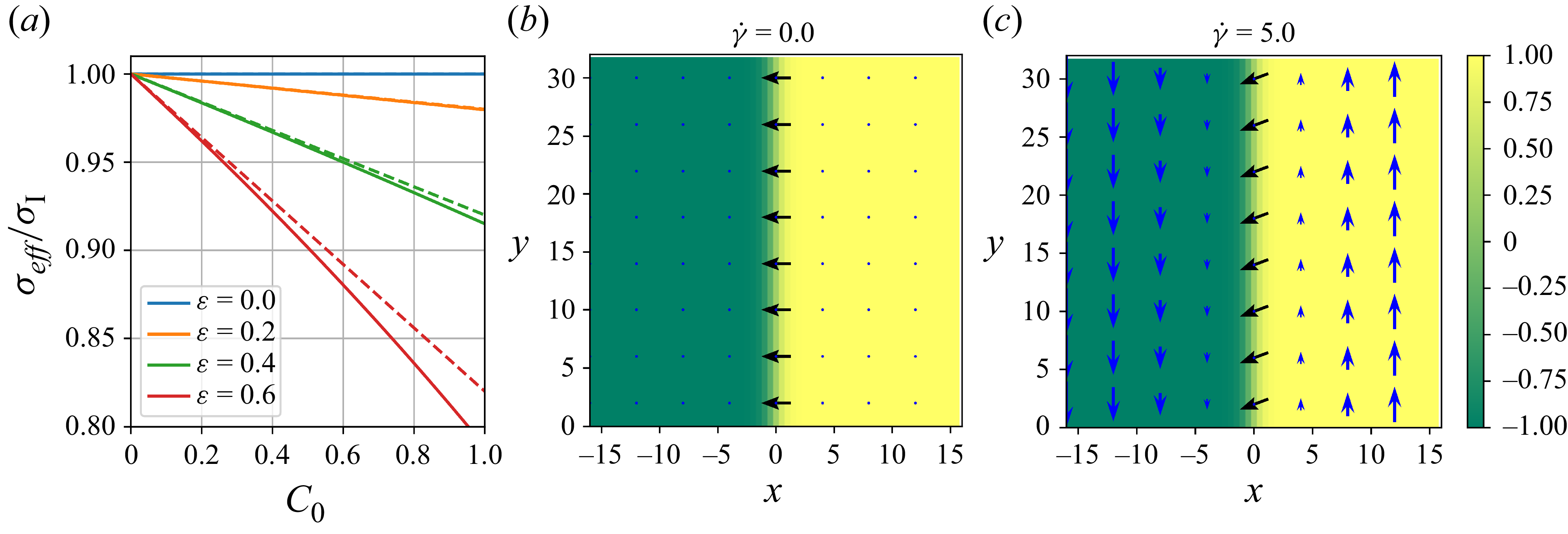
3.3. Adsorption isotherm and effective surface tension
Let us consider a flat interface at
 $x=0$
with
$x=0$
with
 $\phi (x\lt 0)\lt 0$
(water phase) and
$\phi (x\lt 0)\lt 0$
(water phase) and
 $\phi (x\gt 0)\gt 0$
(oil phase), as shown in figure 3(b). The concentration profile
$\phi (x\gt 0)\gt 0$
(oil phase), as shown in figure 3(b). The concentration profile
 $c(x)$
across this interface has been solved perturbatively in (3.11b
) and plotted in figure 2(b). In experiments, the volumetric concentration of surfactant at an oil–water interface is typically
$c(x)$
across this interface has been solved perturbatively in (3.11b
) and plotted in figure 2(b). In experiments, the volumetric concentration of surfactant at an oil–water interface is typically
 $10^2$
–
$10^2$
–
 $10^4$
times larger than the bulk concentration (Faria & Vishnyakov Reference Faria and Vishnyakov2022), far exceeding the interfacial concentrations reached in our simulations. This occurs because real fluid interfaces are extremely sharp: the interfacial width is of the order of a molecular length scale. By contrast, in simulations, we employ a diffuse-interface (phase-field) model, in which the interface is spread over a finite width
$10^4$
times larger than the bulk concentration (Faria & Vishnyakov Reference Faria and Vishnyakov2022), far exceeding the interfacial concentrations reached in our simulations. This occurs because real fluid interfaces are extremely sharp: the interfacial width is of the order of a molecular length scale. By contrast, in simulations, we employ a diffuse-interface (phase-field) model, in which the interface is spread over a finite width
 $\xi _{\textit{I}}$
. For numerical stability and resolution,
$\xi _{\textit{I}}$
. For numerical stability and resolution,
 $\xi _{\textit{I}}$
is usually taken to be several orders of magnitude larger than its physical, molecular-scale value (Jaensson, Hulsen & Anderson Reference Jaensson, Hulsen and Anderson2017). Instead, we quantify adsorption by measuring the amount of surfactant adsorbed per unit interfacial area,
$\xi _{\textit{I}}$
is usually taken to be several orders of magnitude larger than its physical, molecular-scale value (Jaensson, Hulsen & Anderson Reference Jaensson, Hulsen and Anderson2017). Instead, we quantify adsorption by measuring the amount of surfactant adsorbed per unit interfacial area,
 \begin{align} \varGamma = \int _{-\infty }^\infty \left [ c(x) - C_0 \right ] {\textrm{d}}x. \end{align}
Substituting the perturbative solution for
 $c(x)$
in (3.11b
) to (3.20), we obtain
$c(x)$
in (3.11b
) to (3.20), we obtain
 \begin{align} \varGamma = \frac {1}{3}\epsilon ^2 C_0 + \mathcal{O}(\epsilon ^4). \end{align}
Thus, the amount of adsorbed surfactant increases linearly with the bulk concentration
 $C_0$
. This is consistent with the Henry’s law adsorption isotherm in the dilute surfactant limit (van der Sman & van der Graaf Reference van der Sman and van der Graaf2006). A full quantitative comparison with adsorption–desorption kinetics would require extending the model to include finite-rate kinetic terms that explicitly describe the adsorption and desorption of molecules at the interface.
$C_0$
. This is consistent with the Henry’s law adsorption isotherm in the dilute surfactant limit (van der Sman & van der Graaf Reference van der Sman and van der Graaf2006). A full quantitative comparison with adsorption–desorption kinetics would require extending the model to include finite-rate kinetic terms that explicitly describe the adsorption and desorption of molecules at the interface.
We can now compute the reduction in effective surface tension
 $\sigma _{\textit{eff}}$
induced by the adsorption of surfactant molecules at the interface. To do so, we first define the grand potential functional to be
$\sigma _{\textit{eff}}$
induced by the adsorption of surfactant molecules at the interface. To do so, we first define the grand potential functional to be
 \begin{align} \varPhi [\phi ,c,\boldsymbol{p}] = F[\phi ,c,\boldsymbol{p}] - \bar {\mu }_c\int c(\boldsymbol{r})\,d^dr \equiv \int w({\boldsymbol{r}}) \,d^dr, \end{align}
where
 $w(\boldsymbol{r})$
denotes the grand potential density. The constant
$w(\boldsymbol{r})$
denotes the grand potential density. The constant
 $\bar {\mu }_c$
is the chemical potential of an external surfactant reservoir, corresponding to the grand canonical ensemble. Mathematically, the grand potential
$\bar {\mu }_c$
is the chemical potential of an external surfactant reservoir, corresponding to the grand canonical ensemble. Mathematically, the grand potential
 $\varPhi [\phi ,c,\boldsymbol{p}]$
is a Legendre transform of the Helmholtz free energy
$\varPhi [\phi ,c,\boldsymbol{p}]$
is a Legendre transform of the Helmholtz free energy
 $F[\phi ,c,\boldsymbol{p}]$
with respect to
$F[\phi ,c,\boldsymbol{p}]$
with respect to
 $c$
. In equilibrium, the condition
$c$
. In equilibrium, the condition
 $\delta F/\delta c=\bar {\mu }_c$
yields
$\delta F/\delta c=\bar {\mu }_c$
yields
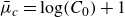 $\bar {\mu }_c=\log (C_0)+1$
. The effective surface tension
$\bar {\mu }_c=\log (C_0)+1$
. The effective surface tension
 $\sigma _{\textit{eff}}$
is then defined to be the excess grand potential per unit area of the interface:
$\sigma _{\textit{eff}}$
is then defined to be the excess grand potential per unit area of the interface:
 \begin{align} \sigma _{\textit{eff}} = \int _{-\infty }^{\infty } \left [ w(x) - w_{\textit{bulk}} \right ]\, {\textrm{d}}x, \end{align}
where
 $w_{\textit{bulk}}$
is the value of the grand potential density evaluated in the bulk, i.e. in the limit
$w_{\textit{bulk}}$
is the value of the grand potential density evaluated in the bulk, i.e. in the limit
 $x\rightarrow \pm \infty$
, or far from the interface. Using the perturbative solutions for
$x\rightarrow \pm \infty$
, or far from the interface. Using the perturbative solutions for
 $\phi (x)$
,
$\phi (x)$
,
 $c(x)$
and
$c(x)$
and
 $p_x(x)$
from § 3.2, (3.23) can then be computed numerically, retaining terms up to order
$p_x(x)$
from § 3.2, (3.23) can then be computed numerically, retaining terms up to order
 $\mathcal{O}(\varepsilon ^6)$
. The resulting effective surface tension
$\mathcal{O}(\varepsilon ^6)$
. The resulting effective surface tension
 $\sigma _{\textit{eff}}$
as a function of the bulk surfactant concentration
$\sigma _{\textit{eff}}$
as a function of the bulk surfactant concentration
 $C_0$
is shown in figure 3(a) (solid lines). As expected,
$C_0$
is shown in figure 3(a) (solid lines). As expected,
 $\sigma _{\textit{eff}}$
approaches the bare interfacial value
$\sigma _{\textit{eff}}$
approaches the bare interfacial value
 $\sigma _{\textit{I}}=2\beta /3$
of the clean binary fluid in the limit
$\sigma _{\textit{I}}=2\beta /3$
of the clean binary fluid in the limit
 $C_0\rightarrow \infty$
. For comparison, we may also invoke the Gibbs adsorption isotherm, which in dimensionless form reads
$C_0\rightarrow \infty$
. For comparison, we may also invoke the Gibbs adsorption isotherm, which in dimensionless form reads
 \begin{align} \frac {{\textrm{d}}\sigma _{\textit{eff}}}{{\textrm{d}}\ln C_0} = -\varGamma . \end{align}
Substituting the expression for
 $\varGamma$
from (3.21) and integrating, we obtain the explicit leading-order result for the effective surface tension
$\varGamma$
from (3.21) and integrating, we obtain the explicit leading-order result for the effective surface tension
 \begin{align} \sigma _{\textit{eff}} = \sigma _{\textit{I}} - \frac {\varepsilon ^2}{3}C_0 + \mathcal{O}(\varepsilon ^4). \end{align}
The corresponding prediction from the Gibbs isotherm is shown in figure 3(a) (dashed lines), where it agrees with our direct definition of
 $\sigma _{\textit{eff}}$
in (3.23).
$\sigma _{\textit{eff}}$
in (3.23).
Finally, we note that the effective surface tension shown in figure 3(a) applies only under equilibrium conditions. At equilibrium, the fluid velocity vanishes
 $\boldsymbol{v}=\boldsymbol{0}$
, and the fluid composition
$\boldsymbol{v}=\boldsymbol{0}$
, and the fluid composition
 $\phi$
, surfactant concentration
$\phi$
, surfactant concentration
 $c$
and polarisation
$c$
and polarisation
 $\boldsymbol{p}$
relax to the configuration which minimises the free energy in (3.1). In this state, the polarisation field
$\boldsymbol{p}$
relax to the configuration which minimises the free energy in (3.1). In this state, the polarisation field
 $\boldsymbol{p}$
aligns strictly perpendicular to the interface, see figure 3(b). In contrast, when the system is subjected to a strong shear flow, for example,
$\boldsymbol{p}$
aligns strictly perpendicular to the interface, see figure 3(b). In contrast, when the system is subjected to a strong shear flow, for example,
 $\boldsymbol{v}\simeq \dot {\gamma }x\hat {\boldsymbol{y}}$
, the polarisation
$\boldsymbol{v}\simeq \dot {\gamma }x\hat {\boldsymbol{y}}$
, the polarisation
 $\boldsymbol{p}$
is oriented by the flow and becomes tilted relative to the interface normal vector, see figure 3(c). This shear-induced reorientation modifies the local interfacial stresses and, consequently, can change the effective surface tension.
$\boldsymbol{p}$
is oriented by the flow and becomes tilted relative to the interface normal vector, see figure 3(c). This shear-induced reorientation modifies the local interfacial stresses and, consequently, can change the effective surface tension.
Plots of binary fluid volume fraction
 $\phi (\boldsymbol{r},t)$
for bare emulsion (a) and surfactant-containing emulsion (b) at different time steps (rows) with values
$\phi (\boldsymbol{r},t)$
for bare emulsion (a) and surfactant-containing emulsion (b) at different time steps (rows) with values
 $t = 10, 110$
and
$t = 10, 110$
and
 $600$
being the first, second and third rows, respectively. The black arrows on the right column indicate the polarisation or average orientation of the surfactant molecules,
$600$
being the first, second and third rows, respectively. The black arrows on the right column indicate the polarisation or average orientation of the surfactant molecules,
 $\boldsymbol{p}(\boldsymbol{r},t)$
. The graphs show that the presence of the surfactants suppresses droplet coalescence and full phase separation. Parameters used:
$\boldsymbol{p}(\boldsymbol{r},t)$
. The graphs show that the presence of the surfactants suppresses droplet coalescence and full phase separation. Parameters used:
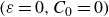 $(\varepsilon =0,C_0=0)$
(a) and
$(\varepsilon =0,C_0=0)$
(a) and
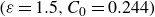 $(\varepsilon =1.5,C_0=0.244)$
(b). Other parameters:
$(\varepsilon =1.5,C_0=0.244)$
(b). Other parameters:
 $\beta =2$
,
$\beta =2$
,
 $B=0.5$
,
$B=0.5$
,
 $M=3$
and
$M=3$
and
 $\gamma _t=\gamma _r=0.01$
.
$\gamma _t=\gamma _r=0.01$
.
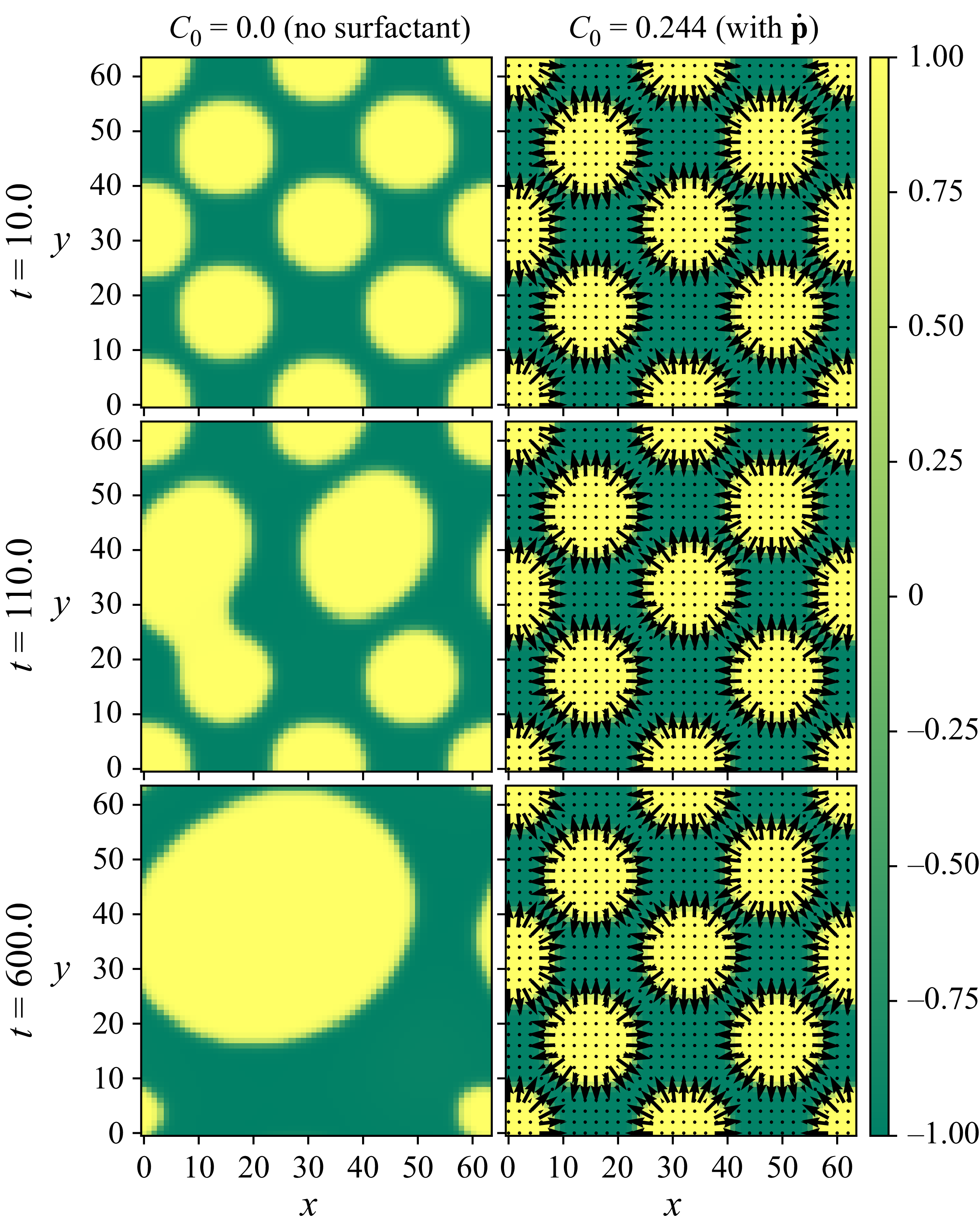
3.4. Emulsion study
Our final case study examines an emulsion of oil droplets suspended in water, with the initial condition shown in the first row of figure 4. Simulations were performed on a
 $L_x\times L_y=64 \times 64$
grid with spatial resolution
$L_x\times L_y=64 \times 64$
grid with spatial resolution
 $\Delta x = \Delta y = 0.5$
and time step
$\Delta x = \Delta y = 0.5$
and time step
 $\Delta t = 0.001$
. To compare the effects of surfactants, we conducted two simulations: one for a clean system with no surfactants (
$\Delta t = 0.001$
. To compare the effects of surfactants, we conducted two simulations: one for a clean system with no surfactants (
 $\varepsilon = 0$
,
$\varepsilon = 0$
,
 $C_0 = 0$
) and one with surfactants present (
$C_0 = 0$
) and one with surfactants present (
 $\varepsilon = 1.5$
,
$\varepsilon = 1.5$
,
 $C_0 = 0.244$
). Periodic boundary conditions were applied along all edges of the domain (
$C_0 = 0.244$
). Periodic boundary conditions were applied along all edges of the domain (
 $x = 0$
,
$x = 0$
,
 $x = L_x$
,
$x = L_x$
,
 $y = 0$
,
$y = 0$
,
 $y = L_y$
).
$y = L_y$
).
In the absence of surfactants, the droplets gradually coalesce into a single large drop. By contrast, when surfactants are present, coalescence is significantly suppressed, leading to a more stable emulsion – although the system will still slowly evolve towards full phase separation over longer time scales. This stabilisation arises from the polarisation field
 $\boldsymbol{p}(\boldsymbol{r},t)$
: the surfactant molecules orient outwards from each droplet, generating effective repulsive interactions that hinder droplet merging. As shown in figure 4, the clean system (figure 4
a) exhibits progressive coalescence, whereas the system with surfactants (figure 4
b) retains a dispersed droplet morphology over the duration of the simulation. Although not shown, we note that increasing the mean surfactant concentration
$\boldsymbol{p}(\boldsymbol{r},t)$
: the surfactant molecules orient outwards from each droplet, generating effective repulsive interactions that hinder droplet merging. As shown in figure 4, the clean system (figure 4
a) exhibits progressive coalescence, whereas the system with surfactants (figure 4
b) retains a dispersed droplet morphology over the duration of the simulation. Although not shown, we note that increasing the mean surfactant concentration
 $C_0$
further suppresses coalescence, much like increasing the interaction strength
$C_0$
further suppresses coalescence, much like increasing the interaction strength
 $\varepsilon$
. Finally, as shown in figure 4(b), the surfactant orientation vectors
$\varepsilon$
. Finally, as shown in figure 4(b), the surfactant orientation vectors
 $\boldsymbol{p}(\boldsymbol{r},t)$
point outwards from each droplet. In this configuration, adjacent droplets effectively experience mutual repulsion due to opposing molecular orientations, thereby maintaining separation and stabilising the emulsion.
$\boldsymbol{p}(\boldsymbol{r},t)$
point outwards from each droplet. In this configuration, adjacent droplets effectively experience mutual repulsion due to opposing molecular orientations, thereby maintaining separation and stabilising the emulsion.
For comparison, we also performed a separate set of simulations in which the polarisation field is treated as quasi-static. In this approximation,
 $\boldsymbol{p}$
is assumed to relax instantaneously to the configuration that minimises the free energy, namely
$\boldsymbol{p}$
is assumed to relax instantaneously to the configuration that minimises the free energy, namely
 \begin{align} \frac {\delta F}{\delta \boldsymbol{p}} = \boldsymbol{0} \quad \Rightarrow \quad \boldsymbol{p} = -\frac {\varepsilon }{2}\boldsymbol{\nabla }\phi . \end{align}
Under weak-flow conditions, where
 $\boldsymbol{v}\simeq \boldsymbol{0}$
, we find no qualitative difference in the stability of the emulsion compared with fully dynamical model shown in figure 4(b). However, in the presence of a strong imposed shear, similar to that in figure 3(c), some quantitative and/or qualitative difference may emerge.
$\boldsymbol{v}\simeq \boldsymbol{0}$
, we find no qualitative difference in the stability of the emulsion compared with fully dynamical model shown in figure 4(b). However, in the presence of a strong imposed shear, similar to that in figure 3(c), some quantitative and/or qualitative difference may emerge.
4. Conclusion
In this work, we have developed a continuum hydrodynamic model for binary-fluid–surfactant systems by systematically deriving both the microscopic and coarse-grained dynamics using Rayleigh’s minimum energy dissipation principle. At the microscopic level, surfactant molecules are modelled as rigid dumbbells that undergo Brownian motion and exert forces and torques on the surrounding fluid due to their amphiphilic character, while the fluid is treated as a continuum field – resulting in a hybrid discrete–continuum formulation. By constructing an appropriate Rayleighian dissipation functional, we derived the overdamped stochastic equations governing the translational and rotational dynamics of individual surfactant molecules.
Upon coarse-graining these microscopic dynamics, we derived a closed set of continuum equations for the surfactant concentration field
 $c(r,t)$
, polarisation field
$c(r,t)$
, polarisation field
 $\boldsymbol{p}(\boldsymbol{r},t)$
, binary fluid composition
$\boldsymbol{p}(\boldsymbol{r},t)$
, binary fluid composition
 $\phi (\boldsymbol{r},t)$
and fluid velocity
$\phi (\boldsymbol{r},t)$
and fluid velocity
 $\boldsymbol{v}(\boldsymbol{r},t)$
. These equations follow consistently from a single mesoscopic free energy functional, ensuring thermodynamic consistency and preserving detailed balance at equilibrium.
$\boldsymbol{v}(\boldsymbol{r},t)$
. These equations follow consistently from a single mesoscopic free energy functional, ensuring thermodynamic consistency and preserving detailed balance at equilibrium.
Our model successfully captures key physical phenomena associated with surfactants, including their accumulation and alignment at interfaces, the reduction of surface tension, and the suppression of droplet coalescence in emulsions. These predictions were validated through a combination of perturbative analytical solutions and direct numerical simulations. Unlike previous approaches, our framework requires no ad hoc stabilising terms, as all interfacial effects and coupling mechanisms emerge naturally from the underlying variational formulation.
Beyond passive surfactants, our formalism is sufficiently general to accommodate additional microscopic ingredients. In particular, the Rayleighian framework and the polarisation dynamics can be readily extended to describe active particles at fluid–fluid interfaces, where self-propulsion, active forces and torques can modify the interfacial stresses (Saintillan & Shelley Reference Saintillan and Shelley2013). This opens the door to studying a broad class of non-equilibrium interfacial phenomena such as active emulsions, self-assembled interfacial monolayers and active Marangoni flows.
Funding
A.J.H. acknowledges EPSRC DTP Studentship No. 2739112. S.C. and E.T. acknowledges funding from EPSRC Grant No. EP/W027194/1. S.M.D. acknowledges London Mathematical Society Undergraduate Research Bursary URB-2024-40.
Declaration of interests
The authors report no conflict of interest.
Use of generative AI
The authors acknowledge the use of generative AI during the preparation of this manuscript for the purpose of improving grammar, enhancing clarity and supporting literature searches. All outputs produced by the tool were carefully checked and revised by the authors, who assume full responsibility for the integrity and accuracy of the published work.
Appendix A. Alternative derivation of the coarse-grained free energy
In §§ 2.1 and 2.2, we derived the free energy functional using the Rayleigh dissipation functional. In this section, we show that one can also derive the free energy functional using direct thermodynamic arguments from Shannon entropy. The total free energy of the system is
 \begin{align} F_{\textit{total}}[\phi ,c,\boldsymbol{p}] = F_{\textit{fluid}}[\phi ] + F_{\textit{surfactants}}[\phi ,c,\boldsymbol{p}] , \end{align}
composed of
 $F_{\textit{fluid}}[\phi ]$
, the free energy contribution from the binary fluid, and
$F_{\textit{fluid}}[\phi ]$
, the free energy contribution from the binary fluid, and
 $F_{\textit{surfactants}}[\phi ,c,\boldsymbol{p}]$
, the free energy contribution from the surfactant molecules. The fluid free energy is taken from standard Cahn–Hilliard theory (Lee et al. Reference Lee, Huh, Jeong, Shin, Yun and Kim2014), while the surfactant contributions are derived using the Helmholtz equation:
$F_{\textit{surfactants}}[\phi ,c,\boldsymbol{p}]$
, the free energy contribution from the surfactant molecules. The fluid free energy is taken from standard Cahn–Hilliard theory (Lee et al. Reference Lee, Huh, Jeong, Shin, Yun and Kim2014), while the surfactant contributions are derived using the Helmholtz equation:
 \begin{align} F_{\textit{surfactants}}[\phi ,c,\boldsymbol{p}] = U[\phi ,c,\boldsymbol{p}] - TS[c,\boldsymbol{p}] , \end{align}
where
 $U$
is the potential energy,
$U$
is the potential energy,
 $T$
is the temperature and
$T$
is the temperature and
 $S$
is the Shannon entropy. The potential energy for the interaction between the molecules and the fluid can be calculated by summing the microscopic energy (second term in (2.8)) over all particles
$S$
is the Shannon entropy. The potential energy for the interaction between the molecules and the fluid can be calculated by summing the microscopic energy (second term in (2.8)) over all particles
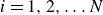 $i=1,2,\ldots N$
, where
$i=1,2,\ldots N$
, where
 $N$
is the total number of particles,
$N$
is the total number of particles,
 \begin{align} U[\phi ,\{\boldsymbol{r}_i,\hat {\boldsymbol{e}}_i\}] = \chi \ell \sum _{i=1}^{N}\hat {\boldsymbol{e}}_i\boldsymbol{\cdot }\boldsymbol{\nabla }_i\phi (\boldsymbol{r}_i). \end{align}
Note that we have ignored higher order terms
 $\sim \ell ^2$
. Equation (A3) can then be coarse-grained straight into its continuum form:
$\sim \ell ^2$
. Equation (A3) can then be coarse-grained straight into its continuum form:
 \begin{align} U[\phi ,c,\boldsymbol{p}] = \int _V \left (\chi \ell c \kern-1.5pt \boldsymbol{p}\boldsymbol{\cdot }\boldsymbol{\nabla }\phi \right ) {\textrm{d}}V, \end{align}
by approximating
 \begin{align} c(\boldsymbol{r},t)\simeq \sum _{i=1}^N \delta (\boldsymbol{r}-\boldsymbol{r}_i) \quad \text{and}\quad c(\boldsymbol{r},t)\boldsymbol{p}(\boldsymbol{r},t) \simeq \sum _{i=1}^N \hat {\boldsymbol{e}}_i\delta (\boldsymbol{r}-\boldsymbol{r}_i). \end{align}
The entropic term can be derived using Shannon’s information entropy expression together with our probability density
 $\psi (\boldsymbol{r},\hat {\boldsymbol{e}},t)$
:
$\psi (\boldsymbol{r},\hat {\boldsymbol{e}},t)$
:
 \begin{align} S[c,\boldsymbol{p}] = -k_{\textit{B}}\int d^dr\int d^{d-1}\hat {e} \, \left [\psi \ln (\mathcal{N}\psi )\right ]. \end{align}
Here,
 $\mathcal{N}$
is a constant ensuring the argument of the logarithm remains dimensionless. This expression can be simplified by representing
$\mathcal{N}$
is a constant ensuring the argument of the logarithm remains dimensionless. This expression can be simplified by representing
 $\psi (\boldsymbol{r},\hat {\boldsymbol{e}},t)$
as a spherical harmonics expansion (see Appendix B):
$\psi (\boldsymbol{r},\hat {\boldsymbol{e}},t)$
as a spherical harmonics expansion (see Appendix B):
 \begin{align} \psi = \frac {1}{S_d}c + \frac {d}{S_d}c \kern-1.5pt \boldsymbol{p}\boldsymbol{\cdot }\hat {\boldsymbol{e}} , \end{align}
where
 $S_d$
is the surface area of a
$S_d$
is the surface area of a
 $d$
-dimensional unit sphere. Higher-order terms are assumed to be negligible. Substituting this into (A6) yields
$d$
-dimensional unit sphere. Higher-order terms are assumed to be negligible. Substituting this into (A6) yields
 \begin{align} S[c,\boldsymbol{p}] &= -\frac {k_{\textit{B}}}{S_d}\int d^dr\int d^{d-1}\hat {e} \left (c + \textit{dc} \kern-1.5pt \boldsymbol{p}\boldsymbol{\cdot }\hat {\boldsymbol{e}}\right )\left [\ln \left (\frac {\mathcal{N}c}{S_d}\right )+\ln \left (1+d\boldsymbol{p}\boldsymbol{\cdot }\hat {\boldsymbol{e}}\right )\right ]. \end{align}
Expanding the second logarithmic term for small
 $\boldsymbol{p}$
gives
$\boldsymbol{p}$
gives
 \begin{align} S[c,\boldsymbol{p}] &= -\frac {k_{\textit{B}}}{S_d}\int d^dr\int d^{d-1}\hat {e} \left [c\ln \left (\frac {\mathcal{N}c}{S_d}\right )\left ( 1+ d\boldsymbol{p}\boldsymbol{\cdot }\hat {\boldsymbol{e}}\right )+dc \kern-1.5pt \boldsymbol{p}\boldsymbol{\cdot }\hat {\boldsymbol{e}} +\frac {1}{2}d^2c\left (\boldsymbol{p}\boldsymbol{\cdot }\hat {\boldsymbol{e}}\right )^2 \right ]. \end{align}
Integrating with respect to
 $\hat {\boldsymbol{e}}$
and using the results from Appendix (B) give us the final expression for the entropic contribution from the surfactants:
$\hat {\boldsymbol{e}}$
and using the results from Appendix (B) give us the final expression for the entropic contribution from the surfactants:
 \begin{align} S[c,\boldsymbol{p}] = -k_{\textit{B}}\int d^dr \left [c\ln \left (\frac {\mathcal{N}}{S_d}c\right )+\frac {d}{2}c|\boldsymbol{p}|^2\right ]{\textrm{d}}V \, . \end{align}
Combining (A4) with this entropy contribution along with the free energy of the fluid
 $F_{\textit{fluid}}[\phi ]$
yields the coarse-grained free energy of (2.36).
$F_{\textit{fluid}}[\phi ]$
yields the coarse-grained free energy of (2.36).
Appendix B. Moment-averaging the single-particle distribution function
We expand the distribution function
 $\psi (\boldsymbol{r}, \hat {\boldsymbol{e}}, t)$
in terms of spherical harmonics as follows:
$\psi (\boldsymbol{r}, \hat {\boldsymbol{e}}, t)$
in terms of spherical harmonics as follows:
 \begin{align} \psi (\boldsymbol{r}, \hat {\boldsymbol{e}}, t)=A_0 c(\boldsymbol{r}, t)+A_1 c(\boldsymbol{r}, t) \boldsymbol{p}(\boldsymbol{r}, t) \boldsymbol{\cdot }\hat {\boldsymbol{e}}+\boldsymbol{\cdot}s . \end{align}
We assume higher order harmonics to be small so we may set
 $A_n=0$
for all
$A_n=0$
for all
 $n \geqslant 2$
. We are now left with two coefficients
$n \geqslant 2$
. We are now left with two coefficients
 $A_0$
and
$A_0$
and
 $A_1$
, which are yet to be determined. To find these coefficients, we need the following results:
$A_1$
, which are yet to be determined. To find these coefficients, we need the following results:
 \begin{align} \int \hat {e}_\alpha \, {\textrm{d}} \varOmega _d & =0 , \end{align}
 \begin{align} \int \hat {e}_\alpha \hat {e}_\beta \, {\textrm{d}} \varOmega _d & =\frac {S_d}{d} \delta _{\alpha \beta } , \end{align}
 \begin{align} \int \hat {e}_\alpha \hat {e}_\beta \hat {e}_\gamma \, {\textrm{d}} \varOmega _d & =0 , \end{align}
 \begin{align} \int \hat {e}_\alpha \hat {e}_\beta \hat {e}_\gamma \hat {e}_\delta \, {\textrm{d}} \varOmega _d & =\frac {S_d}{d(d+2)}\left (\delta _{\alpha \beta } \delta _{\gamma \delta }+\delta _{\alpha \gamma } \delta _{\beta \delta }+\delta _{\alpha \delta } \delta _{\beta \gamma }\right ), \end{align}
where
 $S_d$
is the surface area of the
$S_d$
is the surface area of the
 $d$
-dimensional unit sphere. For example,
$d$
-dimensional unit sphere. For example,
 $S_2=2 \pi$
and
$S_2=2 \pi$
and
 $S_3=4 \pi$
. Now, to find
$S_3=4 \pi$
. Now, to find
 $A_0$
, we integrate (B1) over the solid angle
$A_0$
, we integrate (B1) over the solid angle
 $\varOmega _d$
:
$\varOmega _d$
:
 \begin{align} &\underbrace {\int \psi \,{\textrm{d}} \varOmega _d}_c=A_0 c \underbrace {\int \,{\textrm{d}} \varOmega _d}_{S_d}+A_1 c p_\alpha \underbrace {\int \hat {e}_\alpha \,{\textrm{d}} \varOmega _d}_0\Rightarrow A_0=\frac {1}{S_d}. \end{align}
To find
 $A_1$
, we multiply (B1) by
$A_1$
, we multiply (B1) by
 $\hat {e}_\alpha$
, then integrate over the solid angle
$\hat {e}_\alpha$
, then integrate over the solid angle
 $\varOmega _d$
:
$\varOmega _d$
:
 \begin{align} &\underbrace {\int \psi \hat {e}_\alpha \,{\textrm{d}} \varOmega _d}_{c p_\alpha }=\frac {1}{S_d} c \underbrace {\int \hat {e}_\alpha\, {\textrm{d}} \varOmega _d}_0+A_1 c p_\beta \underbrace {\int \hat {e}_\alpha \hat {e}_\beta \,{\textrm{d}} \varOmega _d}_{\frac {S_d}{d} \delta _{\alpha \beta }} \Rightarrow A_1=\frac {d}{S_d}. \end{align}
Therefore, the truncated spherical expansion for
 $\psi$
can be written as
$\psi$
can be written as
 \begin{align} \psi (\boldsymbol{r}, \hat {\boldsymbol{e}}, t)=\frac {1}{S_d} c(\boldsymbol{r}, t)+\frac {d}{S_d} c(\boldsymbol{r}, t) \boldsymbol{p}(\boldsymbol{r}, t) \boldsymbol{\cdot }\hat {\boldsymbol{e}}. \end{align}
We can use (B5) to find the angular averages
 $\left \langle \hat {e}_\alpha \hat {e}_\beta \right \rangle ,\left \langle \hat {e}_\alpha \hat {e}_\beta \hat {e}_\gamma \right \rangle$
and so on. For instance, to find
$\left \langle \hat {e}_\alpha \hat {e}_\beta \right \rangle ,\left \langle \hat {e}_\alpha \hat {e}_\beta \hat {e}_\gamma \right \rangle$
and so on. For instance, to find
 $\left \langle \hat {e}_\alpha \hat {e}_\beta \right \rangle$
, we use the definition for average:
$\left \langle \hat {e}_\alpha \hat {e}_\beta \right \rangle$
, we use the definition for average:
 \begin{align} \langle \hat {e}_\alpha \hat {e}_\beta \rangle &=\int \psi (\boldsymbol{r}, \hat {\boldsymbol{e}}, t) \hat {e}_\alpha \hat {e}_\beta\, {\textrm{d}} \varOmega _d, \end{align}
which gives
 \begin{align} \langle \hat {e}_\alpha \hat {e}_\beta \rangle &=c\frac {\delta _{\alpha \beta }}{d}, \\[-10pt] \nonumber \end{align}
 \begin{align} \langle \hat {e}_{\alpha }\hat {e}_{\beta }\hat {e}_{\gamma } \rangle &= \frac {c}{d+2}\left (p_{\gamma }\delta _{\alpha \beta } + p_{\beta }\delta _{\alpha \gamma } + p_{\alpha }\delta _{\beta \gamma }\right ). \end{align}
Appendix C. Non-dimensionalisation
In this appendix, we use the bar notation to indicate non-dimensionalised quantities for clarity, however, in the main text, the reverse is true. In the following, we consider the dynamics of coupled surfactant–binary fluid systems in general
 $d$
-dimension. In the simulation, we consider
$d$
-dimension. In the simulation, we consider
 $d=2$
mostly. To get the dimensionless form of the free energy, we introduce
$d=2$
mostly. To get the dimensionless form of the free energy, we introduce
 $\xi _{\textit{I}}=\sqrt {2\kappa /\beta }$
as the unit of length and
$\xi _{\textit{I}}=\sqrt {2\kappa /\beta }$
as the unit of length and
 $k_{\textit{B}}T$
as the unit of energy. Dividing (2.36) by
$k_{\textit{B}}T$
as the unit of energy. Dividing (2.36) by
 $k_{\textit{B}}T$
and rescaling space
$k_{\textit{B}}T$
and rescaling space
 $\boldsymbol{r}=\xi _{\textit{I}}\bar {\boldsymbol{r}}$
, the free energy becomes (note that bars indicate dimensionless quantities)
$\boldsymbol{r}=\xi _{\textit{I}}\bar {\boldsymbol{r}}$
, the free energy becomes (note that bars indicate dimensionless quantities)
 \begin{eqnarray} && \bar {F}=\frac {F}{k_BT}=\int \bigg \{ -\frac {1}{2}\frac {\beta \xi _{\textit{I}}^{d}}{k_{\textit{B}}T}\phi ^{2}+\frac {1}{4}\frac {\beta \xi _{\textit{I}}^{d}}{k_{\textit{B}}T}\phi ^{4}+\frac {1}{2}\frac {\kappa \xi _{\textit{I}}^{d-2}}{k_{\textit{B}}T}|\bar {\boldsymbol{\nabla }}\phi |^{2}+\bar {c}\ln (\bar {c})+\frac {d}{2}\bar {c}|\boldsymbol{p}|^{2} \nonumber\\ && \qquad +\, \frac {\chi \ell }{\xi _{\textit{I}} k_{\textit{B}}T}\bar {c}\boldsymbol{p}\boldsymbol{\cdot }\bar {\boldsymbol{\nabla }}\phi \bigg \} d^{d}\bar {r} \end{eqnarray}
Now, we define the dimensionless parameters to be
 \begin{align} \bar {\beta }=\frac {\beta \xi _{\textit{I}}^{d}}{k_{\textit{B}}T},\quad \bar {\kappa }=\frac {\kappa \xi _{\textit{I}}^{d-2}}{k_{\textit{B}}T}=\frac {\bar {\beta }}{2}\quad \text{and}\quad \varepsilon =\frac {\chi \ell }{\xi _{\textit{I}} k_{\textit{B}}T}, \end{align}
so that the free energy becomes
 \begin{align} \bar {F}=\int \left \{ -\frac {\bar {\beta }}{2}\phi ^{2}+\frac {\bar {\beta }}{4}\phi ^{4}+\frac {\bar {\beta }}{4}|\bar {\boldsymbol{\nabla }}\phi |^{2}+\bar {c}\ln (\bar {c})+\frac {d}{2}\bar {c}|\boldsymbol{p}|^{2}+\varepsilon \bar {c}\boldsymbol{p}\boldsymbol{\cdot }\bar {\boldsymbol{\nabla }}\phi \right \} d^{d}\bar {r}. \end{align}
Now, we introduce
 $\tau$
as the unit of time, so the equations of motion (2.40) become
$\tau$
as the unit of time, so the equations of motion (2.40) become
 \begin{align} \frac {\partial \phi }{\partial \bar {t}}+(\bar {\boldsymbol{v}}\boldsymbol{\cdot }\bar {\boldsymbol{\nabla }}) \phi &= \bar {M} \bar {{\nabla }}^2 \left [-\bar {\beta }\phi + \bar {\beta }\phi ^3 - \frac {\bar {\beta }}{2}\bar {{\nabla} }^2\phi - \varepsilon \bar {\boldsymbol{\nabla }}\boldsymbol{\cdot }(\bar {c}\boldsymbol{p}) \right ], \\[-10pt] \nonumber \end{align}
 \begin{align} \frac {\partial \bar {c}}{\partial \bar {t}}+(\bar {\boldsymbol{v}}\boldsymbol{\cdot }\bar {\boldsymbol{\nabla }})\bar {c} &= \frac {1}{\bar {\gamma }_t}\bar {{\nabla} }^2\bar {c} + \frac {1}{\bar {\gamma }_t} \bar {\boldsymbol{\nabla }} \boldsymbol{\cdot }\left [\bar {c}\bar {\boldsymbol{\nabla }} \left (\frac {d}{2}|\boldsymbol{p}|^2 + \varepsilon \boldsymbol{p}\boldsymbol{\cdot }\bar {\boldsymbol{\nabla }} \phi \right ) \right ], \\[-10pt] \nonumber \end{align}
 \begin{align} \frac {\partial \boldsymbol{p}}{\partial \bar {t}}+(\bar {\boldsymbol{v}}\boldsymbol{\cdot }\bar {\boldsymbol{\nabla }})\boldsymbol{p} &= -\bar {\boldsymbol{\varOmega }}\boldsymbol{\cdot }\boldsymbol{p} - \frac {Bd}{d+2}\bar {\boldsymbol{D}}\boldsymbol{\cdot }\boldsymbol{p} - \frac {d-1}{{\rm d}\bar {\gamma }_r}(d\boldsymbol{p} + \varepsilon \bar {\boldsymbol{\nabla }}\phi ), \end{align}
where we have introduced the dimensionless parameters
 \begin{align} \bar {M}=\frac {Mk_BT\tau }{\xi _{\textit{I}}^{d+2}},\quad \frac {1}{\bar {\gamma }_{t}}=\frac {k_BT\tau }{\gamma _{t}\xi _{\textit{I}}^2}\quad \text{and}\quad \frac {1}{\bar {\gamma }_{r}}=\frac {k_BT\tau }{\gamma _{r}}. \end{align}
The Stokes equation (2.41) becomes
 \begin{align} 0 = -\bar {\boldsymbol{\nabla }}\bar {P} + \bar {\eta }\bar {{\nabla} }^2\bar {\boldsymbol{v}} + \bar {\boldsymbol{f}} + \bar {\boldsymbol{\nabla }}\boldsymbol{\cdot }\bar {\boldsymbol{\sigma }}, \end{align}
where
 $\bar {P}=\xi _{\textit{I}}^dP/(k_{\textit{B}}T)$
is the dimensionless pressure and
$\bar {P}=\xi _{\textit{I}}^dP/(k_{\textit{B}}T)$
is the dimensionless pressure and
 $\bar {\eta }=\eta \xi _{\textit{I}}^d/(\tau k_{\textit{B}}T)$
is the dimensionless viscosity. Here,
$\bar {\eta }=\eta \xi _{\textit{I}}^d/(\tau k_{\textit{B}}T)$
is the dimensionless viscosity. Here,
 $\bar {\boldsymbol{f}}$
and
$\bar {\boldsymbol{f}}$
and
 $\bar {\boldsymbol{\sigma }}$
are the dimensionless force density and stress, respectively:
$\bar {\boldsymbol{\sigma }}$
are the dimensionless force density and stress, respectively:
 \begin{align} \bar {\boldsymbol{f}} &= \frac {\xi ^{d+1}_{\textit{I}}}{k_{\textit{B}}T}\boldsymbol{f} = -\phi \bar {\boldsymbol{\nabla }}\frac {\delta {\bar {F}}}{\delta \phi } -\bar {c}\bar {\boldsymbol{\nabla }}\frac {\delta {\bar {F}}}{\delta \bar {c}} -\boldsymbol{p}\boldsymbol{\cdot }\left (\bar {\boldsymbol{\nabla }}\frac {\delta {\bar {F}}}{\delta \boldsymbol{p}}\right )^T, \\[-10pt] \nonumber \end{align}
 \begin{align} \bar {\boldsymbol{\sigma }} &= \frac {\xi ^d_{\textit{I}}}{k_{\textit{B}}T}\boldsymbol{\sigma } = \frac {Bd}{2(d+2)}\left (\boldsymbol{p}\frac {\delta \bar {F}}{\delta \boldsymbol{p}}+\frac {\delta \bar {F}}{\delta \boldsymbol{p}}\boldsymbol{p}\right )-\frac {1}{2}\left (\boldsymbol{p}\frac {\delta \bar {F}}{\delta \boldsymbol{p}}-\frac {\delta \bar {F}}{\delta \boldsymbol{p}}\boldsymbol{p}\right )\!. \end{align}
Appendix D. Numerical boundary conditions
In our two-dimensional simulation, the space
 $\boldsymbol{r}=(x,y)$
is discretised into
$\boldsymbol{r}=(x,y)$
is discretised into
 $x=i\Delta x$
and
$x=i\Delta x$
and
 $y=j\Delta y$
, where
$y=j\Delta y$
, where
 $i=0,1,2,\ldots N_x-1$
and
$i=0,1,2,\ldots N_x-1$
and
 $j=0,1,2,\ldots N_y-1$
. Here,
$j=0,1,2,\ldots N_y-1$
. Here,
 $N_x$
and
$N_x$
and
 $N_y$
are the number of lattice points along the
$N_y$
are the number of lattice points along the
 $x$
- and
$x$
- and
 $y$
-axis, and
$y$
-axis, and
 $\Delta x$
and
$\Delta x$
and
 $\Delta y$
are the corresponding lattice spacing. The domain size is then
$\Delta y$
are the corresponding lattice spacing. The domain size is then
 $L_x=N_x\Delta x$
along
$L_x=N_x\Delta x$
along
 $x$
and
$x$
and
 $L_y=N_y\Delta y$
along
$L_y=N_y\Delta y$
along
 $y$
. We also discretise the time
$y$
. We also discretise the time
 $t$
into
$t$
into
 $t=n\Delta t$
, where
$t=n\Delta t$
, where
 $n=0,1,2,\ldots$
. The hydrodynamic variables such as
$n=0,1,2,\ldots$
. The hydrodynamic variables such as
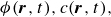 $\phi (\boldsymbol{r},t),c(\boldsymbol{r},t),$
etc. are then discretised into
$\phi (\boldsymbol{r},t),c(\boldsymbol{r},t),$
etc. are then discretised into
 $\phi (\boldsymbol{r},t)\rightarrow \phi ^n_{\textit{ij}}$
, and so on. The
$\phi (\boldsymbol{r},t)\rightarrow \phi ^n_{\textit{ij}}$
, and so on. The
 $\phi$
-dynamics, (3.2a
), can be discretised into
$\phi$
-dynamics, (3.2a
), can be discretised into
 \begin{align} \phi _{\textit{ij}}^{n+1} = \phi ^n_{\textit{ij}} - \Delta t\left (\boldsymbol{\nabla }\boldsymbol{\cdot }\boldsymbol{J}\right )^n_{\textit{ij}} + \Delta t M \left ({\nabla} ^2\mu \right )^n_{\textit{ij}}, \end{align}
where
 $\boldsymbol{J}=\phi \boldsymbol{v}$
and
$\boldsymbol{J}=\phi \boldsymbol{v}$
and
 $\mu =\delta F/\delta \phi =-\beta \phi +\beta \phi ^3-\beta {\nabla} ^2\phi /2-\varepsilon \boldsymbol{\nabla }\boldsymbol{\cdot }(c \kern-1.5pt \boldsymbol{p})$
. Since
$\mu =\delta F/\delta \phi =-\beta \phi +\beta \phi ^3-\beta {\nabla} ^2\phi /2-\varepsilon \boldsymbol{\nabla }\boldsymbol{\cdot }(c \kern-1.5pt \boldsymbol{p})$
. Since
 $\int \phi (\boldsymbol{r},t)\,{\textrm{d}}^2r$
is conserved, we need to ensure that the discretised
$\int \phi (\boldsymbol{r},t)\,{\textrm{d}}^2r$
is conserved, we need to ensure that the discretised
 $\phi _{\textit{ij}}^n$
is also conserved, i.e.
$\phi _{\textit{ij}}^n$
is also conserved, i.e.
 \begin{align} \sum _{i=0}^{N_x-1} \sum _{j=0}^{N_y-1} \phi ^n_{\textit{ij}} = \text{constant for all }n\in \mathbb{Z}. \end{align}
To ensure this, we discretised
 $\boldsymbol{\nabla }\boldsymbol{\cdot }\boldsymbol{J}$
and
$\boldsymbol{\nabla }\boldsymbol{\cdot }\boldsymbol{J}$
and
 ${\nabla} ^2\mu$
as follows:
${\nabla} ^2\mu$
as follows:
 \begin{align} \left (\boldsymbol{\nabla }\boldsymbol{\cdot }\boldsymbol{J}\right )^n_{\textit{ij}} &= \frac {J^n_{x,i+1,j}-J^n_{x,i-1,j}}{2\Delta x} + \frac {J^n_{y,i,j+1}-J^n_{y,i,j-1}}{2\Delta y}, \\[-10pt] \nonumber \end{align}
 \begin{align} \big (\boldsymbol{\nabla} ^2\mu \big )^n_{\textit{ij}} &= \frac {\mu ^n_{i+1,j}+\mu ^n_{i,j}+\mu ^n_{i-1,j}}{\Delta x^2} + \frac {\mu ^n_{i,j+1}+\mu ^n_{i,j}+\mu ^n_{i,j-1}}{\Delta y^2}. \\[10pt] \nonumber \end{align}
We impose the periodic boundary conditions at
 $j=0$
and
$j=0$
and
 $j=N_y-1$
by having
$j=N_y-1$
by having
 \begin{align} \boldsymbol{J}^n_{i,0} = \boldsymbol{J}^n_{i,N_y-1}, \quad \phi ^n_{i,0} = \phi ^n_{i,N_y-1} \quad \text{and}\quad \mu ^n_{i,0} = \mu ^n_{i,N_y-1} \end{align}
for all
 $i$
and
$i$
and
 $n$
. We impose the no-flux boundary conditions at
$n$
. We impose the no-flux boundary conditions at
 $i=0$
and
$i=0$
and
 $i=N_x-1$
by having
$i=N_x-1$
by having
 \begin{align} J^n_{x,0,j} &= -J^n_{x,1,j}, \quad J^n_{x,N_x-1,j} = -J^n_{x,N_x-2,j}, \\[-10pt] \nonumber \end{align}
 \begin{align} \phi ^n_{0,j} &= \phi ^n_{1,j}, \quad \phi ^n_{N_x-1,j} = \phi ^n_{N_x-2,j}, \\[-10pt] \nonumber \end{align}
 \begin{align} \mu ^n_{0,j} &= \mu ^n_{1,j} \quad \text{and}\quad \mu ^n_{N_x-1,j} = \mu ^n_{N_x-2,j} \end{align}
for all
 $j$
and
$j$
and
 $n$
. Similar boundary conditions are also used for
$n$
. Similar boundary conditions are also used for
 $c(\boldsymbol{r},t)$
and
$c(\boldsymbol{r},t)$
and
 $\boldsymbol{p}(\boldsymbol{r},t)$
, except the no-flux condition does not apply to
$\boldsymbol{p}(\boldsymbol{r},t)$
, except the no-flux condition does not apply to
 $\boldsymbol{p}$
.
$\boldsymbol{p}$
.


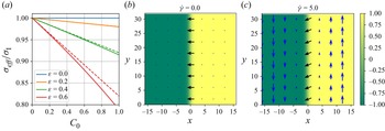


 Open access