1. Introduction

During the Cenozoic era (65 Ma–present), global climate has undergone major changes. In short, the climate’s evolution shifted from an early Cenozoic ‘greenhouse’ into a modern ‘icehouse’ world (e.g. Reference Miller, Fairbanks and MountainMiller and others, 1987; Reference Lear, Elderfield and WilsonLear and others, 2000; Reference Zachos, Pagani, Sloan, Thomas and BillupsZachos and others, 2001). When considering this era, one of the best climate indicators is oxygen isotope records derived from benthic foraminifera (e.g. Reference Zachos, Pagani, Sloan, Thomas and BillupsZachos and others, 2001). These records reflect both deep-sea temperature and the global ice-volume content in time. Figure 1 shows the global mean δ¹⁸O record from Reference Zachos, Pagani, Sloan, Thomas and BillupsZachos and others (2001). The question arises as to which part of this curve describes the temperature and which part is determined by the global ice volume.

Fig. 1.

Global mean benthic oxygen isotope curve smoothed on a 0.1 Myr resolution, from Reference Zachos, Pagani, Sloan, Thomas and BillupsZachos and others (2001). The right axis indicates the corresponding deep-sea temperature when no ice-volume changes are considered.

The evolution of the Antarctic ice sheet (AIS) and the preceding small ice caps on the Antarctic continent, which coalesced into the AIS (in this study all these ice caps are considered as a whole and denoted AIS as well), is an important factor when considering global climate change during the Cenozoic era. It can help to solve the ambiguous interpretation of the global mean benthic oxygen isotope curve. Furthermore, it has major influence on global climate change during the Cenozoic. Geological studies reveal that the Antarctic continent has been situated around the South Pole since the Early Cretaceous (120 Ma) (e.g. Reference BarrettBarrett, 1996), but remained free of a large ice sheet of continental size until 34 Ma. The onset of a large ice sheet of continental size at 34 Ma is clearly shown by records of circum-Antarctic ice-rafted debris found in ocean drilling records (e.g. Reference Zachos, Breza and SherwoodZachos and others, 1992). Furthermore, this event is supported by records of a large sea-level drop (Reference MillerMiller and others, 2005) and a deepening of the calcite compensation depth (Reference Coxall, Wilson, Pälike, Lear and BackmanCoxall and others, 2005). In Figure 1, the steep rise in the oxygen isotope signal of ≈1% at 34 Ma can be largely attributed to the formation of the large AIS of continental size combined with significant cooling (e.g. Reference Coxall, Wilson, Pälike, Lear and BackmanCoxall and others, 2005).

The evolution of the AIS before and even after this onset is not fully understood and is a topic of much debate. Reference MillerMiller and others (2003) show observational evidence for small ice sheets during the Late Cretaceous, about 70 Ma during the Maastrichtian. Before this time the Antarctic continent was probably ice-free (e.g. Reference Francis and PooleFrancis and Poole, 2002; Reference Huber, Norris and MacLeodHuber and others, 2002). During Paleocene and Eocene times, the continent is commonly assumed to have been largely ice-free and partly vegetated, with temperatures well above the freezing point, with highest temperatures around 50 Ma (e.g. Reference BarrettBarrett, 1996; Reference Zachos, Pagani, Sloan, Thomas and BillupsZachos and others, 2001). However, data on this time interval have been sparse and it is unlikely that evidence will be found for high-elevation ice-sheet formation, as the moraines do not reach the coastal region. Recent studies by Reference Coxall, Wilson, Pälike, Lear and BackmanCoxall and others (2005) and Reference Tripati, Backman, Elderfield and FerrettiTripati and others (2005) report evidence for several small glaciations in the middle to late Eocene. That is supported by modeling evidence from Reference DeConto and PollardDeConto and Pollard (2003), who report that small ice sheets (<10⁷ km³) could have formed at high elevations.

After the formation of a large ice sheet at 34 Ma, the ice sheet remained relatively stable during the Oligocene until a period of relative warmth during the Miocene, showing large fluctuations in Antarctic glaciation (e.g. Reference Wright, Miller and FairbanksWright and others, 1992; Reference Williams and HandwergerWilliams and Handwerger, 2005). After 14 Ma, the climate gradually cooled and again large ice sheets formed (e.g. Reference Flower and KennettFlower and Kennett, 1995; Reference Zachos, Pagani, Sloan, Thomas and BillupsZachos and others, 2001).

Numerical models can help to fill the gap between paleoclimatological theories and geological field evidence. Reference OerlemansOerlemans (2004a, Reference Oerlemansb) described how a simple quasi-analytical ice model may be used to correct the Cenozoic oxygen isotope curve for Antarctic ice volume. The model does not explicitly solve the ice dynamics, but instead its evolution is determined by mass continuity of the ice sheet as a whole. The surface of the sheet is defined by a parabolic profile. Sea-level changes are not incorporated. Despite the simplicity of the model, one of its results is that the contributions from both temperature and ice volume to the variability of the oxygen isotope changes are comparable. Furthermore, that modeling study predicts no major ice sheet before 34 Ma.

In this paper, an attempt is made to calculate the Cenozoic evolution of the AIS, by using a one-dimensional ice-flow model which is forced by temperature and sea level. By reconstructing the Cenozoic evolution of the AIS, we will mainly focus on the onset of the large ice sheet at 34 Ma and the present-day conditions of the ice sheet as a whole. The temperature during the Cenozoic is derived from the oxygen isotope proxy after it has been corrected for the ice volume. Furthermore, the model is forced by a Cenozoic global sea-level record (Reference MillerMiller and others, 2005).

In our model we consider the AIS to be axisymmetric and, as an approximation, we use an exponentially decreasing bed. For simplicity, we consider vertically integrated ice dynamics, as we want to integrate over a very long timespan (67.5 Myr). Details of the model and its numerics are discussed in section 2. In section 3 the model is tuned to the present state of the Antarctic ice sheet, and several climate sensitivity experiments are discussed. In section 4 we calculate the Cenozoic evolution of the Antarctic ice sheet by using the global mean oxygen isotope curve from Reference Zachos, Pagani, Sloan, Thomas and BillupsZachos and others (2001) and the Cenozoic sea-level curve from Reference MillerMiller and others (2005), and discuss some sensitivity experiments. In section 5 the resulting deep-sea temperature is presented, and section 6 presents an overall discussion and conclusions.

2. Ice-Flow Model Description

A schematic representation of a cross-section of the ice-sheet model, with several parameters indicated, is presented in Figure 2. The symbols are explained in the text.

Fig. 2.

Schematic representation of ice-sheet cross-section.

2.1. Theory

The ice-flow model is based on the vertically integrated continuity equation. For an axisymmetric ice sheet, with thickness H at distance r from the ice divide, forced by mass balance B, the continuity equation reads (e.g. Reference Van der VeenVan der Veen, 1999)

(1)

with U _r being the vertical mean ice velocity in the radial direction, which is partly the result of deformation, U _δ, and partly the result of sliding, U _s. The velocity due to deformation is expressed by (e.g. Reference Van der VeenVan der Veen, 1999)

(2)

where S _d indicates the driving stress, which is proportional to the ice thickness and slope of the surface. Flow parameter A _d depends, amongst others, on the ice temperature, following an Arrhenius relation (e.g. Reference Van der VeenVan der Veen, 1999). However, as we do not solve the temperature field, this quantity is taken constant and is used as a tuning parameter. The flow-law exponent n is taken as 3. The sliding velocity becomes important near the margin and can be expressed as follows (e.g. Reference Van der VeenVan der Veen, 1999):

(3)

When we assume the basal water pressure P _w to be proportional to the ice load, i.e. P _w = αρ _i gH with α < 1, and the basal shear stress S _b to balance the driving stress, we obtain

(4)

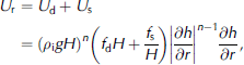
where the surface elevation h is defined by h = H+ b, with bedrock elevation b. Strictly, Equation (4) is valid when H 6≠ 0. In order to restrict the solution when H tends to zero, a small constant ɛ ≪ 1 is added to H. The deformation and sliding parameters, f _d and f _s, are taken as tuning parameters. All parameters and constants are listed in Table 1.

Table 1.

Constants and parameters

The mass balance is calculated following Reference OerlemansOerlemans (2004a), with a small adaptation. The mass balance depends on run-off height h _R. Above this height, the mass balance equals the accumulation rate; below this height, melt also plays a role.

(5)

The accumulation rate A(T _Ant, r) and melt rate –β(Ā)(h _R–h) are described below. We define T _Ant as the mean air temperature reduced to sea level over the Antarctic continent. For the present climate, T _Ant ≈ –18˚C (e.g. Reference Peixoto and OortPeixoto and Oort, 1992). The run-off height can be linearly related to the Antarctic temperature, which is based on observations (Reference OerlemansOerlemans, 2004a).

(6)

The mean accumulation rate Ā depends, through precipitation rate P, strongly on temperature, by means of the moisture-holding capacity of the atmosphere. Furthermore, Ā decreases exponentially with the ice-sheet radius R, representing the fact that large ice sheets will become drier than smaller ones.

(7)

The mass-balance dependency on height is expressed by the mass-balance gradient β. Observations show that this value can be related to the square root of the mean accumulation rate (Reference OerlemansOerlemans, 2001).

(8)

As the model by Reference OerlemansOerlemans (2004a) described the mass continuity of the ice sheet in total, no radial dependency of the accumulation was considered. However, in this study we assume the accumulation rate to increase exponentially outward, as this is more realistic. This small adaptation is calculated following Reference OerlemansOerlemans (2002). The factor c ₃ is used to keep the mean accumulation rate Ā the same as in Reference OerlemansOerlemans (2004a).

(9)

The ice sheet ends where the flotation criterion is met, at the grounding line. Here the ice thickness equals the critical thickness between grounding and flotation, H _gr, depending on the water depth (ζ indicates sea level):

(10)

Ice shelves are not dynamically solved. They have been calculated with the analytical solution by Reference Van der VeenVan der Veen (1999). They do not play a role in solving the dynamics of the ice sheet. During grounding of the ice as a result of sea-level lowering they appear to be too thin to play an important role.

The set of equations is closed by assuming no ice flow at the dome, therefore ∂h/∂r=0|_r=0

As we use an axisymmetric ice-flow model to reconstruct the Cenozoic evolution of the AIS, we need a bed that resembles the ice-free Antarctic bed in one dimension. Elevation is an important factor in ice-sheet formation, due to temperature decrease with height. Build-up of ice to continental sizes is much faster when the underlying bed is flattened (e.g. Reference HuybrechtsHuybrechts, 1993). Coupled climate-modeling studies show that it is plausible that ice caps first formed on higher elevations of Antarctica (Transantarctic Mountains, Dronning Maud Land and Gamburtsev Subglacial Mountains regions) and finally coalesced into the continental ice sheet (e.g. De Conto and Pollard, 2003).

(11)

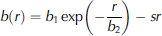
Here we define an exponentially downward-sloping ice-free bed, starting at b ₁ = 2000m in the center. The asymptotic slope s of the oceanic bed is 0.0007. Sea level at present day is set at 0m, which results in a location of the coast at ≈1650km from the center, which is approximately representative for present-day conditions, by assuming the ice sheet’s surface area to be circular. The bed is assumed to adjust to changes in ice loading or sea-level changes. For this a local isostatic depression scheme is used (a so-called LLRA (local-lithosphere–relaxed-asthenosphere) scheme) (Reference Le Meur and HuybrechtsLe Meur and Huybrechts, 1996).

It is important to note that the model is forced by only one temperature, T _Ant , and by sea level ζ.

2.2. Numerical implementation

The model is solved with a finite-difference approach, on a so-called staggered grid of type II (Reference Huybrechts and PayneHuybrechts and others, 1996). The ice thickness on every gridpoint results from integration in time of the continuity equation, Equation (1). The mass balance is calculated on every gridpoint, whereas the mass flux is determined exactly in between the gridpoints, in order to calculate the flux divergence exactly at the gridpoints. The integration in time is calculated with an implicit Cranck–Nicholson scheme. After integration, the grounding line is determined, by checking for which gridpoints the ice column grounds or floats (Equation (10)).

In order to integrate over a long time-span like the Cenozoic, one wants to avoid small time-steps in order to restrict the computing time. For this reason, and in order to prevent numerical instabilities, the spatial grid distance cannot be too small and must be at least 10 km. However, following this restriction, the grounding line cannot respond in an appropriate way to climate change (see also Reference Vieli and PayneVieli and Payne, 2005). This is illustrated in Figure 3. Here a constant grid is assumed, where k ₀ indicates the numerical grounding line, i.e. the last gridpoint before flotation occurs. For grid distances of >10 km, the ice thickness at this location can be several hundreds of meters when we consider ice sheets of continental size. If one assumes, for example, a sea-level drop, it is easy to let the ice sheet grow further. However, due to ice thickness of several hundreds of meters at the numerical grounding line, now located at gridpoint k0 + 1, a huge step in sea-level rise must be taken to let the sheet retreat to its original size. As a result, a strong hysteresis effect occurs. Grid spacings larger than 10 km are much too large to solve the migration of the grounding zone of large ice sheets numerically.

Fig. 3.

(a) Schematic ice-sheet response to sea-level drop of 100 m. (b) Ice-sheet response to sea-level rise back to the original sea level.

Hence, we use a stretching grid, and adjust the grid size Δr at every time-step. This is done in such a way that the position of the grounding line, determined by the flotation criterion, is located exactly halfway between two adjacent gridpoints. This is accomplished by a linear extrapolation of the ice thickness starting at r _k0 , the location of the last gridpoint which is grounded.

(12)

The location r at which the extrapolated ice thickness H(r) equals the critical ice thickness, determined by the flotation criterion, indicates the grounding line and is set exactly halfway between two gridpoints. This determines the new grid size, and all fields are converted onto this new grid. In this way the growth or retreat of the ice sheet is directly related to water depth, and the model is therefore necessarily sensitive to climate change. The ice flux across the grounding line, F _gr, is easily calculated, as the ice thickness and surface slope are known at this location.

It is necessary to keep the grid spacing between specified boundaries, in order to prevent numerical instabilities (Reference Van den Berg, van de Wal and OerlemansVan den Berg and others, 2006), when the integration time-step is kept constant. Therefore the grid size Δr is restricted between 18 and 20 km, and the integration time-step Δt = 1 year. The total number of gridpoints is 200.

3. Climate Sensitivity

Various flow and bed parameters are chosen in such a way that the present ice sheet’s radius and volume (T _Ant = –18˚C, R = 1925 km, V = 26×10⁶ km³, dome–coast distance ≈ 1650 km) are simulated. The bed parameters are given in section 2.1, whereas the other parameters are listed in Table 1.

The equilibrium radius and volume and the mass flux components, for different temperatures, are plotted in Figure 4a and b. Sea level is taken to be constant. Starting with an ice-free configuration in warm conditions, ice-sheet formation initiates at the highest bedrock elevations by lowering the temperature. This initiation occurs at T _Ant = 6˚C. Further cooling results in a lower melt rate and a consequently larger mass balance near the edge, which results in a larger ice sheet. This increases the total amount of accumulation and melt. The ice sheet reaches the coast at T _Ant = –1˚C. For lower temperatures, rapid build-up of ice occurs as the melt rate further decreases. The mass flux at the grounding line increases, due to the growth of the ice thickness at the grounding line. The maximum ice-sheet volume is reached at T _Ant = –7˚C. For lower temperatures the ice sheet becomes smaller due to decreasing moisture content in the atmosphere. The sensitivity of the model for low temperatures is small, as the flux across the grounding line acts as a strong stabilizing mechanism due to the large sensitivity of this quantity to ice thickness.

Fig. 4.

(a) Equilibrium ice-sheet volume (solid line) and radius (dashed line) against Antarctic temperature T _Ant. Present-day values are indicated by dots. The location of the coast is indicated by the dotted line. (b) Components of the total mass flux against temperature: total accumulation (solid line), total melt (dashed line) and total mass flux at grounding line, F _gr (dash-dotted line).

The results are compared to model results obtained by Reference OerlemansOerlemans (2004a) and Reference HuybrechtsHuybrechts (1993). Oerlemans used a simple quasi-analytical model, forced by the mass-balance parameterization on which our mass balance is based, except for the radial dependency of the accumulation rate. Huybrechts used a three-dimensional ice-flow model including thermodynamics, on a realistic ice-free bedrock topography, which is adapted from the present orography. However, the mass-balance formulation is different. It is not useful to compare the three models in detail, as the formulations are completely different. In short, one can state that the gradual build-up is comparable, but our model initiates at higher temperatures than Oerlemans (<–5˚C) and Huybrechts (<2˚C). This is mostly related to the differences in bed profiles. Furthermore, the ice-sheet profile of Oerlemans is predefined, resulting in a steeper and thinner profile compared to our profiles, which are the result of flow dynamics. This thinning in the grounding zone has a large effect on the melt rate, resulting in a smaller ice sheet. Finally, our model shows a comparable sensitivity for low temperatures compared to Huybrechts.

The sensitivity of the model to sea-level change is plotted in Figure 5. As we define T _Ant as the mean Antarctic temperature at sea level, it is important to discriminate between a fixed temperature field and a temperature field which moves relative to sea-level change. The last method is applied here, as we considered this case to be more realistic. However, the results show small differences between the two cases.

Fig. 5.

Response to sea-level change for different temperature regimes: T _Ant = –25˚C, –18˚C, –10˚C, –3˚C, 0˚C and 5˚C.

The sea level is forced from –100 towards 100 m, with respect to the present day, for various temperatures. The response to sea-level change is calculated by shifting the Antarctic temperature as well, where a lapse rate of –0.007 K per meter of sea-level change is assumed. As the global ocean spans about 70% of the Earth’s surface, sea-level changes can be considered to account effectively for only 70% of this temperature shift. However, we assume a temperature shift of 100%, which can be considered to result in a maximum effect. Figure 5 shows the sensitivity to sea-level change for several Antarctic temperatures at 0 m. For the low-temperature regime (<–7˚C), a sea-level rise results in a decreasing ice sheet, determined by the flotation criterion. However, due to the coupling between the temperature field and sea-level change, a sea-level rise results in a temperature rise as well, forcing an ice-sheet growth for this temperature regime. This effect counteracts the sea-level sensitivity in a limited way. For the high-temperature regime, the ice sheet does not reach the coastal region, which excludes the flotation effect. When the sea level drops, an ice sheet only shrinks due to this temperature effect, thus making even small ice caps sensitive to sea-level change.

4. Reconstruction of Cenozoic Ice Volume

The ice-flow model, as described above, is used in order to split the δ¹⁸O signal into a deep-sea temperature and an ice-volume record. This is done in the same way as described in Reference OerlemansOerlemans (2004a). The simplest way to relate the δ¹⁸O record to the deep-sea temperature T _ds and ice volume V is a linear relation

(13)

with parameters a = 2.625% and b = –0.25%K^–1 (e.g. Reference Zachos, Pagani, Sloan, Thomas and BillupsZachos and others, 2001). The parameter c depends on the ratio of the mean isotopic composition of ice sheets relative to that of the ocean. This value depends on temperature, which implies that c is not constant during the Cenozoic. Nevertheless as a first approximation c can be considered constant and is assumed to be c = 0.4×10^–16m^–3% (e.g. Reference Zachos, Pagani, Sloan, Thomas and BillupsZachos and others, 2001), implying that the present-day AIS causes a shift of 1% in the benthic δ¹⁸O record.

First, sea level is kept constant, so that the ice-flow model is forced by the mean Antarctic temperature at sea level alone. This quantity can be related to the global mean temperature at sea level T _sl as follows:

(14)

Δ₀ represents a typical offset between the Antarctic continent and global mean sea-level temperature without the Antarctic ice sheet, and determines the strength of cooling due to the presence of an ice sheet, which is related to the ice surface area (αR ²; R _p indicates the present-day radius). is about 5–10 K in order to meet the present difference between the polar temperatures in the Northern and Southern Hemispheres (e.g. Reference Peixoto and OortPeixoto and Oort, 1992; Reference OerlemansOerlemans, 2004a).

The benthic oxygen isotope record (Fig. 1) changes under the influence of the deep-sea temperature T _ds. Nowadays, deep-sea temperatures reflect approximately the mean surface temperature at high latitudes, as deep water is formed at high latitudes. For the Cenozoic this probably does not hold anymore, as the thermohaline circulation has been changing under several influences (e.g. Reference Crowley and NorthCrowley and North, 1991). For lack of knowledge, we assume that changes in the global mean deep-sea temperatures reflect changes in the global mean surface temperatures. The discrepancy between the deep-sea temperature and the global mean surface temperature can be incorporated in Δ₀, resulting in the previously unknown constant Δ. This makes Equation (14)

(15)

Before we can split the oxygen isotope curve into its deep-sea temperature part and its Antarctic ice volume part, the curve must be corrected for ice-sheet formation in the Northern Hemisphere, which is done by subtracting a linear function, from 0% at 2 Ma to 0.8% in the late Pleistocene. The oxygen isotope curve can now be split, by using Equations (13) and (15) simultaneously. On every new time-step the deep-sea temperature is adjusted to the calculated ice volume during the former time-step. We used ice-free starting conditions, but similar results are obtained when using present-day starting conditions. Δ and are used as a tuning parameters and are considered to be 0–10 K (Δ) and 5–10 K (η) and are kept constant in time during a complete Cenozoic run.

The resulting ice-sheet radius and volume for several values of Δ are plotted in Figure 6a and b respectively. For these runs is set at8K. For all cases, ice sheets do exist when the Cenozoic era starts at 65 Ma. Only for large Δ (>5 K), when the temperature is low enough, are these Paleocene and Eocene ice sheets of continental size. Around 50 Ma, the ice sheets reach their minimal size. Later on, during the Eocene, the sheet grows again and reaches its continental size at different ages, depending on Δ. Only for Δ = 0, 1, or 2 K (when is set at8K) does this growth occur at 34 Ma. When is smaller and set at 5 K, Δ can be at most 5 K in order to fit the continental offset at 34 Ma. During the Oligocene, the ice sheet remains more or less stable and about the same size for Δ≥1. During the Miocene, several scenarios are possible. For small values of Δ or , the ice sheet shrinks and becomes land-based. For larger values, the Miocene fluctuations are much smaller and the ice sheet remains of continental size. In the late Miocene (<13 Ma) the ice sheet reaches its continental size again for all values of Δ.

Fig. 6.

(a) Ice-sheet radius against age during the Cenozoic run, Δ = 0–3 K, = 8K. The straight dotted line indicates the coast. (b) Volume reconstruction for the same parameters. (c) Resulting ice flux across the grounding line. (d) Resulting Antarctic temperature. (a) and (d) also show the results for Δ = 10 K, =8K. The black dot indicates the present-day value of T _Ant.

As already noted in the introduction, evidence of the onset of the large AIS at 34 Ma is, amongst others, found in marine sediment records by circum-Antarctic ice-rafted debris (e.g. Reference Zachos, Breza and SherwoodZachos and others, 1992). This quantity is probably proportional to the ice flux across the grounding line, F _gr, which is plotted in Figure 6c. Only for Δ = 1 or 2 K does the flux not start before 34 Ma and it immediately reaches large values (more than half of present-day values). When Δ becomes larger than 2 K, the initiation starts earlier, which geological studies suggest is unlikely. The flux almost vanishes in the Miocene till 15 Ma, and gradually increases towards present-day values or even more. When Δ = 0 K, the flux is probably too small to fit the observed ice-rafted debris.

The calculated Antarctic temperatures are plotted in Figure 6d. As expected, ice sheets of continental size show up when T _Ant drops below –1˚C. The calculated present-day temperature however, does not resemble the observed value of –18˚ C. This is plausible according to Equation (15), since Δ + must be ≈18 K for present-day conditions. In order to meet this condition, Δ should be in the range ˚–13 K, provided that varies between 5 and 10 K. However, this does not match with the required continental size initiation at 34 Ma, as for these larger values of Δ the initiation will be much too early, compared to observations. This is shown in Figure 6a for Δ = 10 K. As our model is not extremely sensitive to temperature change in the low-temperature range, the resulting present-day volumes are about the same and we assume that the condition of matching the present-day temperature is of less importance than the condition of initiation of a continental-sized ice sheet at 34 Ma, when we assume Δ to be constant in time. However, it is more likely that Δ varied substantially during the Cenozoic. Due to the decrease of CO₂ over millions of years, the global temperature decreases. It seems plausible that the Antarctic temperature decreases more rapidly than the deep-sea temperature, due to the global representativeness of the latter and the fact that this quantity is restricted. This results in a larger difference between T _ds and T _Ant , so it is plausible that Δ will increase in time. For present-day conditions, this parameter is about 10 K, when =8K. In order to meet the criterion at 34 Ma, Δ cannot be larger than about 2 K. In between, the evolution of Δ(t) is not known. If we assume a linear relation, restrictions on ice volume both at 34 Ma and at the present day are met. In between, the fluctuations during the Miocene became much smaller than when Δ was set at 2 K. Maybe the large increase of Δ towards the present-day value occurred mostly after the Miocene. Furthermore, it is not likely that was much larger than the present-day value of 5–10 K, even for high CO₂ concentration scenarios, which is caused by the albedo feedback on temperature.

In the remaining part we focus on the results obtained with Δ = 2 K and = 8K.

As a first approximation, we assumed c to be constant, implying that the mean isotopic content of ice with respect to that of the ocean remains constant. However, the isotopic content of ice depends on differences in temperature during the fractionation process during evaporation and condensation. In order to test whether this effect significantly influences the results as described above, several model runs were performed for which parameter c was assumed to be proportional to the difference between the Antarctic temperature and deep-sea temperature. The maximum variation in c was set at 25%, a relatively large upper limit (Reference Bintanja, van de Wal and OerlemansBintanja and others, 2005). The results show that this effect is negligible when considering the evolution of the AIS and thus c may be considered constant.

Furthermore, the influence of sea-level height, as provided by the reconstruction by Reference MillerMiller and others (2005), was incorporated. This was investigated with a sea-level-dependent temperature field (see section 3). The results are plotted in Figure 7. It is shown that the ice-sheet evolution is influenced in a minor way. In the early Cenozoic until 34 Ma, sea level was much higher than at present. However, the ice sheet did not reach the coastal region and thus was not restricted by sea level or growing due to increasing water depth. The model shows a slightly smaller volume for this period, due to the warming effect of sea-level rise. This results in a smaller ice sheet for high temperatures (>–7˚C). During the warm period at 52 Ma, the ice sheet almost vanishes as the sea level rises to 140 m. If Δ = 1 K the continent even became ice-free during this period, until the equilibrium line dropped below the elevation of the summit of the continent. After 34 Ma, the ice sheet is restricted by sea level, and fluctuations are not large until 5 Ma, consistent with sea-level fluctuations of at most 40 m. From that moment, the ice sheet grows due to significant cooling and the resulting sea-level drop.

Fig. 7.

(a) Global sea-level curve by Reference MillerMiller and others (2005). (b) Modeled ice-sheet volume, model forced by Cenozoic δ¹⁸O record (Reference Zachos, Pagani, Sloan, Thomas and BillupsZachos and others, 2001) and Cenozoic sea-level record (Reference MillerMiller and others (2005) (solid line), together with results due to δ¹⁸O forcing alone (dashed line). Δ = 2 K and = 8K.

5. Resulting Deep-Sea Temperature Record

We present the resulting deep-sea temperature in Figure 8. The dashed line shows the deep-sea temperature for ice-free conditions, i.e. V = 0km³ in Equation (13), while the solid line shows the resulting deep-sea temperature for Δ = 2 K and =8K. At 34 Ma, the temperature drops about 2 K, which contributes to about half of the total shift in δ¹⁸O. This temperature drop ends when the Miocene starts, and the deep-sea temperature then remains more or less constant until 15 Ma, after which it gradually cools till the end of the Miocene, with a rapid cooling during the Pliocene and Quaternary. The resulting deep-sea temperature during Paleocene and Eocene times is not lower than 6˚C and reaches its maximum value of about 11.5˚C at 50 Ma. The values are significantly higher than for ice-free conditions (dashed line), which is the direct result of the formation of small ice sheets up to 10⁷ km³. Also the temperature record derived from Mg/Ca from Reference Lear, Elderfield and WilsonLear and others (2000) is added, which is not influenced by ice-volume effects. After 25 Ma, our result matches reasonably well with this Mg/Ca curve, which implies that the reconstructed ice volume is nicely reproduced for this period.

Fig. 8.

Resulting deep-sea temperature for Δ = 2 K and = 8K (solid line) together with the paleotemperature curve derived from Mg/Ca in benthic foraminiferal calcite (Reference Lear, Elderfield and WilsonLear and others, 2000) (dash-dotted line). The dashed line indicates the non-corrected deep-sea temperature derived from Reference Zachos, Pagani, Sloan, Thomas and BillupsZachos and others (2001). This curve is calculated by taking V = 0km³ in Equation (13).

6. Discussion and Conclusions

In order to reconstruct the Antarctic ice sheet during Cenozoic times with an ice-flow model, one needs a model which is not too complex and which is most likely solved on a coarse grid O(10km). Furthermore, it must be sensitive to climate changes. This can be accomplished by using a vertically integrated axisymmetrical ice-flow model, solved on a grid which is stretched to the size of the ice sheet.

When the model is forced with the Cenozoic oxygen isotope curve, the two well-known conditions, i.e. the initiation of a large ice sheet at 34Ma and present-day temperature of –18˚C, are not met for a single parameter setting, when these parameters are assumed to be constant. This can be attributed to the small sensitivity at low temperatures. When Δ is time-dependent, both conditions can be met. However, the temporal relation of this variable is unknown.

The resulting ice-sheet volume is achieved for low values of Δ. When is assumed to be8K, Δ is supposed not to be larger than 2 K. This is smaller than the value for present-day conditions (≈10 K), as the difference between the global temperature at sea level and the Antarctic temperature, corrected for the ice sheet’s presence, is much larger than the difference between the global temperature at sea level and the global mean deep-sea temperature (e.g. Reference Peixoto and OortPeixoto and Oort, 1992).

All possible solutions show the presence of an ice sheet during the entire Cenozoic, which has its smallest size at 50 Ma. This seems plausible, as there is evidence for the presence of ice sheets of about 5–10×10⁶ km³ during the Maastrichtian (≈70 Ma) (Reference MillerMiller and others, 2003). Due to temperature rise, the amount of ice will gradually shrink, but even during the warmest period at 55–50Ma the existence of small ice caps is predicted in high mountainous regions.

During the Late Oligocene (27–23.5 Ma), the ice sheet retreats such that the flux across the grounding line vanishes. However, the ice volume is still 60% of the present-day volume, in line with recent estimates by Reference Pekar and DeContoPekar and DeConto (2006). During this period, ice-volume changes contribute up to 50% of the change in the marine signal. A near-complete collapse of the AIS around 25 Ma, as suggested by Reference Zachos, Pagani, Sloan, Thomas and BillupsZachos and others (2001), is therefore not necessary to explain the marine δ¹⁸O record. As the resulting flux across the grounding line almost vanishes, marine sediment cores do not reveal much of the ice sheet’s presence.

Sea-level changes appear to be of minor importance when we focus on the entire Cenozoic evolution. When the temperature field is influenced by sea-level changes, the ice volume is slightly smaller before 34 Ma, as the sea level is relatively high. During the very warm period around 50 Ma, the ice sheet became very small or may have vanished. After initiation of the large ice sheet, sea-level changes caused only small fluctuations of the ice-sheet volume.

The results are compared to Reference OerlemansOerlemans (2004b). Oerlemans reports values of Δ = 9 K and = 5 K. The main difference is the existence of a small ice sheet during Early Cenozoic times, which is much smaller (<2×106^km3) in Reference OerlemansOerlemans (2004b). This is caused by the difference in Δ, which is the direct result of the shift in temperature for gradual ice-sheet build-up (Fig. 4), due to the different ice-sheet profile. The Miocene variations are larger in Oerlemans’ study, resulting in smaller deep-sea temperatures.

The resulting deep-sea temperature shows similarities with the Mg/Ca curve by Reference Lear, Elderfield and WilsonLear and others (2000) after 25 Ma. This supports the idea that the calculated ice volume during this period is in the proper range.

The difference between the ice-free temperature record and the modeled record during Paleocene and Eocene times is directly related to the possible existence of small ice sheets. Some climate-modeling studies report discrepancies between data and modeled temperatures (e.g. Reference Bice and MarotzkeBice and Marotzke, 2002; Reference Huber, Sloan and ShellitoHuber and others, 2003). This favors the idea that there may have been substantial ice sheets during the Paleocene and Eocene, as in that case the marine record should be corrected for ice volume. This leads to higher deep-sea temperatures than generally assumed (Fig. 8).