





1. Introduction
From bubbly drinks (Zenit & Rodríguez-Rodríguez Reference Zenit and Rodríguez-Rodríguez2018) to volcanic eruptions (Oppenheimer et al. Reference Oppenheimer, Capponi, Cashman, Lane, Rust and James2020), multiphase flows are ubiquitous in both nature and everyday life. One of the simplest examples is the emptying of a bottle of water, wine or beer. As air has to go through the bottleneck to replace the liquid leaving the vessel, it creates a periodic flow, characterised by the well-known onomatopoeia ‘glug-glug’, very different from the predictable Torricelli flow (Torricelli Reference Torricelli1644), although the transition between the two regimes has been explored (Schwefler, Nienaber & Mayer Reference Schwefler, Nienaber and Mayer2023). Early studies of large bubbles rising in closed tubes provide a first insight into this simple yet rich physical system (Dumitrescu Reference Dumitrescu1943; Davies & Taylor Reference Davies and Taylor1950; Zukoski Reference Zukoski1966). The draining of bottles has since been investigated in a variety of configurations, from commercial bottles (Whalley Reference Whalley1987, Reference Whalley1991; Geiger, Velten & Methner Reference Geiger, Velten and Methner2012; Mayer Reference Mayer2019; Rohilla & Das Reference Rohilla and Das2020; Nguyen, Gichigi & Mayer Reference Nguyen, Gichigi and Mayer2023) to simplified geometries called ‘ideal bottles’, which consist of a cylindrical tank with a flat bottom to avoid the complexity of the bottleneck. They have been studied both experimentally (Schmidt & Kubie Reference Schmidt and Kubie1995; Kubie Reference Kubie1999; Clanet & Searby Reference Clanet and Searby2004) and numerically (Mer et al. Reference Mer, Praud, Neau, Merigoux, Magnaudet and Roig2018, Reference Mer, Praud, Magnaudet and Roig2019; Bhattacharya & Lakkaraju Reference Bhattacharya and Lakkaraju2024). Some experiments have also been conducted to study the effect of the bottleneck by adding a cylindrical tube of varying length at the exit of the vessel (Tehrani, Patrick & Wragg Reference Tehrani, Patrick and Wragg1992; Kubie Reference Kubie1998; Koukouvaos & Kubie Reference Koukouvaos and Kubie2001). A common empirical observation across these studies is that the velocity of the free surface at the air–liquid interface remains constant during the drainage.
To our knowledge, no previous studies have investigated the draining of a suspension from a bottle, be it ideal or not. Several works have focused on the draining of particles from an immersed silo or hopper (Wilson et al. Reference Wilson, Pfeifer, Mesyngier and Durian2013; Koivisto & Durian Reference Koivisto and Durian2017). A surge in the emptying rate has been reported near the end of the draining process, attributed to the interstitial fluid being pumped faster as a result of the dilation of grains close to the exit. This mechanism can be interpreted as a particle-induced pressure sucking the liquid toward the outlet, as described by Kulkarni, Metzger & Morris (Reference Kulkarni, Metzger and Morris2010) in viscous regimes. Consequently, the suspension downstream of the constriction becomes progressively less concentrated as more fluid leaves the vessel. In this sense, the suspension is self-filtrating while going through the bottleneck. This phenomenon, known as self-filtration or self-dilution (Marin & Souzy Reference Marin and Souzy2025), has not been studied in the case of particle-to-hole diameter ratio slightly smaller than but close to $1$
. This is the regime in which immersed particles flowing through a constriction can accumulate around the opening, form an arch and hinder the flow. This phenomenon, known as clogging, differs from jamming, which corresponds to a global state of arrest of the system whereas clogging is a local process (Zuriguel & Garcimartín Reference Zuriguel and Garcimartín2022). Such events can be mitigated by placing an obstacle in front of the exit, applying external vibrations to the suspension or allowing for a fluid counter-current flow (see Marin & Souzy Reference Marin and Souzy2025 and references within). A closely related situation arises in dry granular media, where clogging may induce oscillatory drainage similar to the ‘glug-glug’ regime mentioned above. In that case, air intermittently enters through the exit to compensate for the discharged grains (Wu et al. Reference Wu, Måløy, Hansen, Ammi and Bideau1993). This parallel further highlights the central role played by the interstitial fluid, whether liquid or gas, in controlling the drainage dynamics.
$1$
. This is the regime in which immersed particles flowing through a constriction can accumulate around the opening, form an arch and hinder the flow. This phenomenon, known as clogging, differs from jamming, which corresponds to a global state of arrest of the system whereas clogging is a local process (Zuriguel & Garcimartín Reference Zuriguel and Garcimartín2022). Such events can be mitigated by placing an obstacle in front of the exit, applying external vibrations to the suspension or allowing for a fluid counter-current flow (see Marin & Souzy Reference Marin and Souzy2025 and references within). A closely related situation arises in dry granular media, where clogging may induce oscillatory drainage similar to the ‘glug-glug’ regime mentioned above. In that case, air intermittently enters through the exit to compensate for the discharged grains (Wu et al. Reference Wu, Måløy, Hansen, Ammi and Bideau1993). This parallel further highlights the central role played by the interstitial fluid, whether liquid or gas, in controlling the drainage dynamics.
In this study, we experimentally investigate the emptying dynamics of a bottle containing suspended particles. Although the orifice-to-particle diameter ratio ranges from approximately two to ten, clogging is never observed in our system. The periodic entry of bubbles prevents the formation of stable particle arches that could obstruct the bottleneck. In the following, we describe the experimental set-up, the range of explored parameters and initial observations in § 2. Section 3 presents experimental results, in particular the flow rate variations with these parameters; it also introduces a model adapted from Clanet & Searby (Reference Clanet and Searby2004), which links the flow rate to the rise velocity of the bubbles. § 4 focuses on the unexpected accumulation of particles inside the bottle, leading, for high packing fractions, to their emergence above the liquid free surface. Finally, § 5 concludes this work and opens some perspectives.
2. Experimental method
2.1. Experimental set-up
The ideal bottle consists of a cylindrical vessel with a height of $L = {447}\,\mathrm{mm}$
and a diameter
$L = {447}\,\mathrm{mm}$
and a diameter $d_0 = {110}\,\mathrm{mm}$
for a capacity of approximately
$d_0 = {110}\,\mathrm{mm}$
for a capacity of approximately ${4.25}\,\mathrm{l}$
. The set-up for all the experiments described in this article is sketched in figure 1. The top of the bottle is sealed and its bottom has a circular hole with a variable diameter
${4.25}\,\mathrm{l}$
. The set-up for all the experiments described in this article is sketched in figure 1. The top of the bottle is sealed and its bottom has a circular hole with a variable diameter $d$
. In this study, three different hole diameters were used,
$d$
. In this study, three different hole diameters were used, $d \in \{{20}\,\mathrm{mm}; {30}\,\mathrm{mm} ; {40}\,\mathrm{mm} \}$
, hereafter referred to as d20, d30 and d40, respectively. Note that the hole opening is bevelled outward to mitigate the teapot effect (Kistler & Scriven Reference Kistler and Scriven1994; Duez et al. Reference Duez, Ybert, Clanet and Bocquet2010).
$d \in \{{20}\,\mathrm{mm}; {30}\,\mathrm{mm} ; {40}\,\mathrm{mm} \}$
, hereafter referred to as d20, d30 and d40, respectively. Note that the hole opening is bevelled outward to mitigate the teapot effect (Kistler & Scriven Reference Kistler and Scriven1994; Duez et al. Reference Duez, Ybert, Clanet and Bocquet2010).
Sketch of the experimental set-up. An ideal bottle of height $L$
and diameter
$L$
and diameter $d_0$
is filled with a suspension and then emptied through a hole of variable diameter
$d_0$
is filled with a suspension and then emptied through a hole of variable diameter $d$
at the bottom. The mass of suspension drained out of the bottle is measured with a force sensor. A camera allows for a direct visualisation of the drainage. The pressure difference between the top of the bottle and the atmosphere is measured with a pressure sensor. Here,
$d$
at the bottom. The mass of suspension drained out of the bottle is measured with a force sensor. A camera allows for a direct visualisation of the drainage. The pressure difference between the top of the bottle and the atmosphere is measured with a pressure sensor. Here, $g=9.81\,\textrm{ms}^{-2}$
is the gravitational acceleration.
$g=9.81\,\textrm{ms}^{-2}$
is the gravitational acceleration.

A force sensor (Honeywell 152) and a basin act as a balance to measure the mass $m(t)$
of the liquid and particles exiting the bottle during an experiment. The signal is sampled at
$m(t)$
of the liquid and particles exiting the bottle during an experiment. The signal is sampled at ${1000}\,\mathrm{Hz}$
. A camera (Chronos 2.1), together with a light panel located behind the cell, allows for direct visualisation of the suspension drainage including the position of the free surface
${1000}\,\mathrm{Hz}$
. A camera (Chronos 2.1), together with a light panel located behind the cell, allows for direct visualisation of the suspension drainage including the position of the free surface $z(t)$
, the particles exiting the bottle, the liquid jet and the bubbles rising. The frame rate is 200 fps for the d40 hole and 100 fps for the d30 and d20 holes. Finally, a pressure sensor (MKS Instruments, 223 BD-00010 AB) is placed inside the bottle, above the initial suspension level. It measures the pressure difference
$z(t)$
, the particles exiting the bottle, the liquid jet and the bubbles rising. The frame rate is 200 fps for the d40 hole and 100 fps for the d30 and d20 holes. Finally, a pressure sensor (MKS Instruments, 223 BD-00010 AB) is placed inside the bottle, above the initial suspension level. It measures the pressure difference $\Delta P (t)$
between the atmosphere and the air at the top of the vessel.
$\Delta P (t)$
between the atmosphere and the air at the top of the vessel.
2.2. Suspensions
The different types of spherical particles used in this study are presented in table 1. They are made of either polyamide or hydrogel, with diameters $d_p$
ranging from
$d_p$
ranging from ${5}\,\mathrm{}$
to
${5}\,\mathrm{}$
to ${17}\,\mathrm{mm}$
(see figure 2). The ratio
${17}\,\mathrm{mm}$
(see figure 2). The ratio $d/d_p$
ranges then from 1.8 to 6. Note that for systems in which there is no air entrainment, such as an open vessel or a purely liquid–solid system, clogging events would take place in a significant part of this
$d/d_p$
ranges then from 1.8 to 6. Note that for systems in which there is no air entrainment, such as an open vessel or a purely liquid–solid system, clogging events would take place in a significant part of this $d/d_p$
range (Marin & Souzy Reference Marin and Souzy2025). In order to obtain quasi-isodense suspensions, the density of the fluid is matched to that of the particles within a few per cent, the residual mismatch arising from small bead-to-bead density variations due to inhomogeneities in the manufactured particles. The density is noted
$d/d_p$
range (Marin & Souzy Reference Marin and Souzy2025). In order to obtain quasi-isodense suspensions, the density of the fluid is matched to that of the particles within a few per cent, the residual mismatch arising from small bead-to-bead density variations due to inhomogeneities in the manufactured particles. The density is noted $\rho$
and corresponds to the density of the fluid. Under these conditions, the volume fraction equals the mass fraction within the density-matching tolerance. The chosen suspending liquid is either salt water or a water/UCON
$\rho$
and corresponds to the density of the fluid. Under these conditions, the volume fraction equals the mass fraction within the density-matching tolerance. The chosen suspending liquid is either salt water or a water/UCON $^{\textit{TM}}$
mixture. UCON
$^{\textit{TM}}$
mixture. UCON $^{\textit{TM}}$
(75-H-90000) is an industrial lubricant miscible with water. It was used for the density matching of hydrogel beads suspensions instead of salt water as the latter fractures the hydrogel beads. The quantity added to pure water is less than 5 % and the viscosity increases up to
$^{\textit{TM}}$
(75-H-90000) is an industrial lubricant miscible with water. It was used for the density matching of hydrogel beads suspensions instead of salt water as the latter fractures the hydrogel beads. The quantity added to pure water is less than 5 % and the viscosity increases up to ${2 \times 10^{-3}}\,\mathrm{Pa\,s}$
. The initial suspension packing fraction is denoted
${2 \times 10^{-3}}\,\mathrm{Pa\,s}$
. The initial suspension packing fraction is denoted $\phi _0$
.
$\phi _0$
.
Characteristics of the particles used for the suspensions.

Particles used for the suspensions. From left to right: polyamide beads $\sim \hspace {-0.1cm}{10}\,\mathrm{mm}$
(PA10), polyamide beads
$\sim \hspace {-0.1cm}{10}\,\mathrm{mm}$
(PA10), polyamide beads $\sim \hspace {-0.1cm}{5}\,\mathrm{mm}$
(PA5), hydrogel beads
$\sim \hspace {-0.1cm}{5}\,\mathrm{mm}$
(PA5), hydrogel beads $\sim \hspace {-0.1cm}{10}\,\mathrm{mm}$
(H10), hydrogel beads
$\sim \hspace {-0.1cm}{10}\,\mathrm{mm}$
(H10), hydrogel beads $\sim \hspace {-0.1cm}{17}\,\mathrm{mm}$
(H17). The scale is the same for all images. The characteristics of the particles are presented in table 1.
$\sim \hspace {-0.1cm}{17}\,\mathrm{mm}$
(H17). The scale is the same for all images. The characteristics of the particles are presented in table 1.

2.3. Protocol
Before starting an experiment, the plate with the hole of the chosen diameter $d$
is screwed to the bottom of the bottle. The hole is sealed with a rubber plug. The top of the bottle is opened to fill the vessel with first the suspending liquid and then the particles in adequate proportion to reach the required particle volume fraction
$d$
is screwed to the bottom of the bottle. The hole is sealed with a rubber plug. The top of the bottle is opened to fill the vessel with first the suspending liquid and then the particles in adequate proportion to reach the required particle volume fraction $\phi _0$
, ranging from 0 to 60 % depending on the experiment. The suspension is slowly stirred inside the container, which is then closed before starting the drainage. The method of filling has not been found to substantially change the measured physical quantities. The suspension initially occupies the vessel up to a height
$\phi _0$
, ranging from 0 to 60 % depending on the experiment. The suspension is slowly stirred inside the container, which is then closed before starting the drainage. The method of filling has not been found to substantially change the measured physical quantities. The suspension initially occupies the vessel up to a height $h_0$
. Note that some deviations are observed from the isodense assumption. Although the suspension is stirred before closing the container, during the few seconds before starting the experiments, some particles can either float or sink (in most cases, as we match the average density, both are observed). This is due to slight inhomogeneities in the particle density (see § 2.2). However, after opening, the rising bubbles and fluid recirculation quickly homogenise the suspension. The top cover includes the pressure sensor.
$h_0$
. Note that some deviations are observed from the isodense assumption. Although the suspension is stirred before closing the container, during the few seconds before starting the experiments, some particles can either float or sink (in most cases, as we match the average density, both are observed). This is due to slight inhomogeneities in the particle density (see § 2.2). However, after opening, the rising bubbles and fluid recirculation quickly homogenise the suspension. The top cover includes the pressure sensor. $m_0$
denotes the initial mass of suspension in the bottle and
$m_0$
denotes the initial mass of suspension in the bottle and $m_{p,0}$
is the initial mass of particles. Hence, the initial packing fraction is
$m_{p,0}$
is the initial mass of particles. Hence, the initial packing fraction is $\phi _0 = m_{p,0}/m_0$
. The basin and force sensor are positioned below the exit.
$\phi _0 = m_{p,0}/m_0$
. The basin and force sensor are positioned below the exit.
At time $t=0$
, the rubber plug is manually removed and the experiment begins. At the end, when no more liquid or particles exit the bottle for a few seconds, the total mass of particles that exited the bottle
$t=0$
, the rubber plug is manually removed and the experiment begins. At the end, when no more liquid or particles exit the bottle for a few seconds, the total mass of particles that exited the bottle $m_{p,end}$
is separated from the liquid and weighed on a scale.
$m_{p,end}$
is separated from the liquid and weighed on a scale.
2.4. First observations
Typical measurements of a suspension drainage (PA10, $\phi _0 = 10\,\%$
, d30,
$\phi _0 = 10\,\%$
, d30, $h_0\,=\,{21}\,\mathrm{cm}$
,
$h_0\,=\,{21}\,\mathrm{cm}$
, $m_0 = {2.25}\,\mathrm{kg}$
). The figure displays the normalised mass
$m_0 = {2.25}\,\mathrm{kg}$
). The figure displays the normalised mass $m(t)/m_0$
of the suspension exiting the bottle (in black) and the normalised pressure difference
$m(t)/m_0$
of the suspension exiting the bottle (in black) and the normalised pressure difference $\Delta P(t)/\rho g h_0$
between the top of the bottle and the atmosphere (in grey) as a function of time
$\Delta P(t)/\rho g h_0$
between the top of the bottle and the atmosphere (in grey) as a function of time $t$
. The linear trends (dashed lines) are obtained by a linear fit. Inset: zoom on the pressure signal (black box on the main signal) to show the periodic pressure oscillations.
$t$
. The linear trends (dashed lines) are obtained by a linear fit. Inset: zoom on the pressure signal (black box on the main signal) to show the periodic pressure oscillations.

As an example, we present the draining of a $\phi _0 = 10\,\%$
suspension of PA10 through an exit hole of
$\phi _0 = 10\,\%$
suspension of PA10 through an exit hole of ${30}\,\mathrm{mm}$
, with an initial height
${30}\,\mathrm{mm}$
, with an initial height $h_0 = {21}\,\mathrm{cm}$
and an initial mass
$h_0 = {21}\,\mathrm{cm}$
and an initial mass $m_0 = {2.25}\,\mathrm{kg}$
. Figure 3 displays the temporal evolution of the normalised mass
$m_0 = {2.25}\,\mathrm{kg}$
. Figure 3 displays the temporal evolution of the normalised mass $m(t)/m_0$
of the suspension drained out of the bottle (in black) and of the normalised pressure difference
$m(t)/m_0$
of the suspension drained out of the bottle (in black) and of the normalised pressure difference $\Delta P(t)/\rho g h_0$
between the inside of the bottle and the atmosphere (in grey), where
$\Delta P(t)/\rho g h_0$
between the inside of the bottle and the atmosphere (in grey), where $\rho$
is the fluid density and
$\rho$
is the fluid density and $g=9.81\,\textrm{ms}^{-2}$
is the gravitational acceleration.
$g=9.81\,\textrm{ms}^{-2}$
is the gravitational acceleration.
The mass evolution shows a global linear increase, $\overline {m}(t)$
, superimposed with large amplitude variations. These fluctuations correspond to the coupled effects of liquid jet and particle impacts, together with the intrinsic dynamic response of the force sensor, leading to significant high-frequency noise. Examining the fluctuations of
$\overline {m}(t)$
, superimposed with large amplitude variations. These fluctuations correspond to the coupled effects of liquid jet and particle impacts, together with the intrinsic dynamic response of the force sensor, leading to significant high-frequency noise. Examining the fluctuations of $m(t) - \overline {m}(t)$
shows only very minor differences between the cases
$m(t) - \overline {m}(t)$
shows only very minor differences between the cases $\phi _0 = 0\,\%$
and
$\phi _0 = 0\,\%$
and $\phi _0 = 50\,\%$
, making the analysis of these fluctuations inconclusive. The mass flow rate
$\phi _0 = 50\,\%$
, making the analysis of these fluctuations inconclusive. The mass flow rate $Q_m$
is defined as the slope of the linear fit of the mass evolution. In figure 3, the slope of the white dashed line is
$Q_m$
is defined as the slope of the linear fit of the mass evolution. In figure 3, the slope of the white dashed line is $Q_m/m_0$
. From here, the volumetric flow rate is computed as
$Q_m/m_0$
. From here, the volumetric flow rate is computed as $Q_V = Q_m/\rho$
. The linear fit is performed over the whole experiment and we can write
$Q_V = Q_m/\rho$
. The linear fit is performed over the whole experiment and we can write
 \begin{align} \overline {m}(t) = Q_m t. \end{align}
Note that the value of the flow rate does not change significantly if the linear fit is made on a smaller interval as long as it is longer than the characteristic time scales of the periodic flow and the sensor’s response. For all experiments within the range of parameters explored, the flow rate is found to be constant. No particle clogging is observed in any of the experiments, as the suspension always exits the vessel. The entrance of air bubbles is sufficient to break any arches that would form, even for $d/d_p \approx 2$
. To evaluate the error associated with the choice of a linear model, other polynomial fits were performed. The linear fit deviates from higher-order fits by approximately 5 %. Hence, we take 5 % as the uncertainty on the measured flow rate for all packing fractions.
$d/d_p \approx 2$
. To evaluate the error associated with the choice of a linear model, other polynomial fits were performed. The linear fit deviates from higher-order fits by approximately 5 %. Hence, we take 5 % as the uncertainty on the measured flow rate for all packing fractions.
Example of a suspension drainage (PA10, $\phi _0 = 10\,\%$
, d30,
$\phi _0 = 10\,\%$
, d30, $h_0={21}\,\mathrm{cm}, m_0\,=\,{2.25}\,\mathrm{kg}$
). (a) Chronophotograph of the experiment (see Movie 1 is available at https://doi.org/10.1017/jfm.2026.11646). The free surface is indicated by the horizontal red dashed line. (b) Intensity averaged along the horizontal axis,
$h_0={21}\,\mathrm{cm}, m_0\,=\,{2.25}\,\mathrm{kg}$
). (a) Chronophotograph of the experiment (see Movie 1 is available at https://doi.org/10.1017/jfm.2026.11646). The free surface is indicated by the horizontal red dashed line. (b) Intensity averaged along the horizontal axis, $\langle I(x,z,t)\rangle _x$
, as a function of time
$\langle I(x,z,t)\rangle _x$
, as a function of time $t$
. The colour bar indicates the intensity, from 0 to 255, with yellow indicating light and blue indicating dark. The linear trend of the free-surface evolution is shown by the dashed red line. The stars identify the time of each picture in (a). Before the opening of the bottle, particles are floating or sinking since the density is not matched perfectly. Rising bubbles and fluid recirculation then quickly homogenise the suspension, as indicated by the uniformity of the colour blue during the drainage. As the polyamide particles are opaque, they hinder the visualisation of rising bubbles, which is not the case for hydrogel beads (see figures 6 and 9).
$t$
. The colour bar indicates the intensity, from 0 to 255, with yellow indicating light and blue indicating dark. The linear trend of the free-surface evolution is shown by the dashed red line. The stars identify the time of each picture in (a). Before the opening of the bottle, particles are floating or sinking since the density is not matched perfectly. Rising bubbles and fluid recirculation then quickly homogenise the suspension, as indicated by the uniformity of the colour blue during the drainage. As the polyamide particles are opaque, they hinder the visualisation of rising bubbles, which is not the case for hydrogel beads (see figures 6 and 9).

After the plug is removed, the pressure difference drops to a value close to the hydrostatic equilibrium as the pressure at the bottom is imposed to be the atmospheric pressure. Afterwards, the signal oscillates with a typical period $T$
(see Appendix A) around a linear trend (black dashed line in figure 3), which is still due to the hydrostatic pressure, as
$T$
(see Appendix A) around a linear trend (black dashed line in figure 3), which is still due to the hydrostatic pressure, as $\Delta P (t) \approx -\rho g z(t)$
. The observed oscillations are caused by the formation of bubbles at the bottom of the bottle. Indeed, when a bubble enters the bottle, it pushes the column of suspension up. Then, when the suspension is ejected, the column moves down, and so on. The amplitude of oscillations changes during the experiment, possibly due to foam coalescing, bubbles bursting or events that strongly disturb the interface (see Movie 1).
$\Delta P (t) \approx -\rho g z(t)$
. The observed oscillations are caused by the formation of bubbles at the bottom of the bottle. Indeed, when a bubble enters the bottle, it pushes the column of suspension up. Then, when the suspension is ejected, the column moves down, and so on. The amplitude of oscillations changes during the experiment, possibly due to foam coalescing, bubbles bursting or events that strongly disturb the interface (see Movie 1).
Snapshots of the experiment are displayed for three different times in figure 4(a) (see Movie 1). From the images taken by the camera, the light intensity is averaged along the horizontal $x$
-axis. This intensity vector represents the mean intensity along the horizontal as a function of the vertical coordinate
$x$
-axis. This intensity vector represents the mean intensity along the horizontal as a function of the vertical coordinate $z$
,
$z$
, $\langle I(x,z,t)\rangle _x$
. This process is applied to all the images and results in figure 4(b), which displays a spatio-temporal diagram of the drainage. The free surface is easily noticeable as it marks the separation between the dark suspension (in blue) and the light background (in yellow). Before the opening of the bottle, particles are floating or sinking since the density is not matched perfectly. Rising bubbles and fluid recirculation then quickly homogenise the suspension as indicated by the uniformity of the colour blue during the draining. In this example, the fluid level in the bottle decreases linearly (dashed red line, figure 4
b), as expected. Indeed, volume conservation imposes that the flow rate
$\langle I(x,z,t)\rangle _x$
. This process is applied to all the images and results in figure 4(b), which displays a spatio-temporal diagram of the drainage. The free surface is easily noticeable as it marks the separation between the dark suspension (in blue) and the light background (in yellow). Before the opening of the bottle, particles are floating or sinking since the density is not matched perfectly. Rising bubbles and fluid recirculation then quickly homogenise the suspension as indicated by the uniformity of the colour blue during the draining. In this example, the fluid level in the bottle decreases linearly (dashed red line, figure 4
b), as expected. Indeed, volume conservation imposes that the flow rate $Q_V$
and the free-surface velocity
$Q_V$
and the free-surface velocity $v_S$
are linearly linked. The volume exiting the bottle from below is equal to the decreasing volume inside the bottle:
$v_S$
are linearly linked. The volume exiting the bottle from below is equal to the decreasing volume inside the bottle: $Q_V = S_0 v_S$
with
$Q_V = S_0 v_S$
with $S_0 = \pi d_0^2/4$
being the cross-sectional area of the bottle.
$S_0 = \pi d_0^2/4$
being the cross-sectional area of the bottle.
3. Suspension drainage
3.1. Influence of particles on the flow rate
As the flow rate is constant, its dependence on the experimental parameters (diameter of the exit hole, size and material of the particles, initial packing fraction) is studied. The initial height $h_0$
of suspension in the bottle is chosen not to change the flow rate value within the experimental range, as expected from Schmidt & Kubie (Reference Schmidt and Kubie1995). Figure 5 shows the flow rate
$h_0$
of suspension in the bottle is chosen not to change the flow rate value within the experimental range, as expected from Schmidt & Kubie (Reference Schmidt and Kubie1995). Figure 5 shows the flow rate $Q_V$
as a function of the initial volume fraction
$Q_V$
as a function of the initial volume fraction $\phi _0$
for the different experimental conditions. First, without particles (
$\phi _0$
for the different experimental conditions. First, without particles ( $\phi _0 = 0$
), increasing the hole diameter leads to a strong increase in the flow rate, as expected. Then, for a given suspension and hole diameter, the flow rate slightly decreases as the initial packing fraction increases. This is true for all
$\phi _0 = 0$
), increasing the hole diameter leads to a strong increase in the flow rate, as expected. Then, for a given suspension and hole diameter, the flow rate slightly decreases as the initial packing fraction increases. This is true for all $\phi _0$
tested, even at
$\phi _0$
tested, even at $60\,\%$
packing fraction, where we would expect that the possible formation of arches around the hole would greatly decrease the flow rate. In fact, the formation of bubbles inside the bottle prevents the creation of any arches. This is very different from the emptying of viscous fluids where the value of the flow rate decreases strongly with viscosity (Monnet Reference Monnet2024). This observation interferes with the use of any effective fluid model for the suspensions as the effective viscosity would diverge near
$60\,\%$
packing fraction, where we would expect that the possible formation of arches around the hole would greatly decrease the flow rate. In fact, the formation of bubbles inside the bottle prevents the creation of any arches. This is very different from the emptying of viscous fluids where the value of the flow rate decreases strongly with viscosity (Monnet Reference Monnet2024). This observation interferes with the use of any effective fluid model for the suspensions as the effective viscosity would diverge near $\phi _0 = 60\,\%$
(Guazzelli & Pouliquen Reference Guazzelli and Pouliquen2018). Instead, the dynamics is controlled by collisions between particles and bubbles, as expected for bubbles having the same size as the particles (Hooshyar et al. Reference Hooshyar, van Ommen, Hamersma, Sundaresan and Mudde2013). In this particular set-up, the particles are pushed outside the centre. Under these conditions, a Reynolds number for the flow can be computed as
$\phi _0 = 60\,\%$
(Guazzelli & Pouliquen Reference Guazzelli and Pouliquen2018). Instead, the dynamics is controlled by collisions between particles and bubbles, as expected for bubbles having the same size as the particles (Hooshyar et al. Reference Hooshyar, van Ommen, Hamersma, Sundaresan and Mudde2013). In this particular set-up, the particles are pushed outside the centre. Under these conditions, a Reynolds number for the flow can be computed as $ \textit{Re} = Q_V/{d}\nu \approx 10^4$
near the hole, with
$ \textit{Re} = Q_V/{d}\nu \approx 10^4$
near the hole, with $\nu \approx {10^{-6}}\,\mathrm{m^2 \, s}^{-1}$
being the kinematic viscosity of the liquid. Besides, the size and material of the particles do not appear to have a significant impact on the flow rate. However, draining experiments conducted with deformable beads (H10 and H17) demonstrate a higher flow rate than the one with hard beads (PA10 and PA5).
$\nu \approx {10^{-6}}\,\mathrm{m^2 \, s}^{-1}$
being the kinematic viscosity of the liquid. Besides, the size and material of the particles do not appear to have a significant impact on the flow rate. However, draining experiments conducted with deformable beads (H10 and H17) demonstrate a higher flow rate than the one with hard beads (PA10 and PA5).
Flow rate $Q_V$
as a function of the suspension’s initial particle volume fraction
$Q_V$
as a function of the suspension’s initial particle volume fraction $\phi _0$
for all the experiments. The size of the markers corresponds to the diameter of the particles (see table 1). The shape of the marker codes for the material of the particles (squares for hydrogel and circles for polyamide). The intensity of the marker colour corresponds to the diameter of the exit hole (light colours for small and dark colours for large).
$\phi _0$
for all the experiments. The size of the markers corresponds to the diameter of the particles (see table 1). The shape of the marker codes for the material of the particles (squares for hydrogel and circles for polyamide). The intensity of the marker colour corresponds to the diameter of the exit hole (light colours for small and dark colours for large).

3.2. Revisiting Clanet & Searby’s (2004) model
To describe these variations with $\phi _0$
, we follow the same reasoning as in Clanet & Searby (Reference Clanet and Searby2004). As the typical time
$\phi _0$
, we follow the same reasoning as in Clanet & Searby (Reference Clanet and Searby2004). As the typical time $T$
(
$T$
( $\approx {0.2}\,\mathrm{s}$
) between the formation of two bubbles is small compared with the time of emptying
$\approx {0.2}\,\mathrm{s}$
) between the formation of two bubbles is small compared with the time of emptying $T_e$
(a few tens of seconds), we assume that the two phenomena are decoupled. To evaluate the mass evolution
$T_e$
(a few tens of seconds), we assume that the two phenomena are decoupled. To evaluate the mass evolution $\overline {m}(t)$
at large time scale, we can therefore ignore the flow oscillations due to the alternation between bubbles entering the bottle and liquid jets exiting the vessel. Let us consider the air in the vessel above the suspension as an ideal gas undergoing an isothermal transformation, as the variations in temperature are negligible during our experiments. At all times, we can write
$\overline {m}(t)$
at large time scale, we can therefore ignore the flow oscillations due to the alternation between bubbles entering the bottle and liquid jets exiting the vessel. Let us consider the air in the vessel above the suspension as an ideal gas undergoing an isothermal transformation, as the variations in temperature are negligible during our experiments. At all times, we can write $P(t) V(t) = N(t) k_B \varTheta$
, where
$P(t) V(t) = N(t) k_B \varTheta$
, where $P(t)$
is the air pressure,
$P(t)$
is the air pressure, $V(t)$
is its volume,
$V(t)$
is its volume, $N(t)$
is the number of gas particles and
$N(t)$
is the number of gas particles and $\varTheta$
is the temperature. In our set-up, we measure
$\varTheta$
is the temperature. In our set-up, we measure $\Delta P(t)$
corresponding to the pressure difference between the air inside the bottle and the ambient air, as illustrated in figure 3. We thus have
$\Delta P(t)$
corresponding to the pressure difference between the air inside the bottle and the ambient air, as illustrated in figure 3. We thus have $P(t) = P_0 + \Delta P(t)$
, with
$P(t) = P_0 + \Delta P(t)$
, with $\Delta P(t) \approx \rho g L \approx {5 \times 10^3}\,\mathrm{Pa} \ll P_0$
. Therefore, we consider
$\Delta P(t) \approx \rho g L \approx {5 \times 10^3}\,\mathrm{Pa} \ll P_0$
. Therefore, we consider $P(t) \approx P_0$
. Differentiating the ideal gas relation with respect to time leads to
$P(t) \approx P_0$
. Differentiating the ideal gas relation with respect to time leads to
 \begin{align} \frac {\text{d}V}{\text{d}t} = \frac {\text{d}N}{\text{d}t} \frac {k_B \varTheta }{P_0}. \end{align}
Air arriving at the top of the bottle is coming from bubbles entering through the hole. The typical volume of a bubble is denoted $V_b$
and the number of gas particles per bubble is
$V_b$
and the number of gas particles per bubble is $N_b$
. A bubble enters the bottle at atmospheric pressure and temperature, so
$N_b$
. A bubble enters the bottle at atmospheric pressure and temperature, so $P_0 V_b = N_b k_B \varTheta$
. The number of gas particles entering the bottle by unit of time is
$P_0 V_b = N_b k_B \varTheta$
. The number of gas particles entering the bottle by unit of time is $\mathrm{d}N/\mathrm{d}t \approx N_b/T$
. During a cycle of length
$\mathrm{d}N/\mathrm{d}t \approx N_b/T$
. During a cycle of length $T$
, the bubble enters the bottle at a typical velocity
$T$
, the bubble enters the bottle at a typical velocity $v_b$
, during a time
$v_b$
, during a time $\alpha T$
(with
$\alpha T$
(with $0 \lt \alpha \lt 1$
) and with a typical cross-section equal to the cross-section of the hole
$0 \lt \alpha \lt 1$
) and with a typical cross-section equal to the cross-section of the hole $s = \pi d^2/4$
(see figure 14 in Clanet & Searby Reference Clanet and Searby2004). Hence, the volume of a bubble is
$s = \pi d^2/4$
(see figure 14 in Clanet & Searby Reference Clanet and Searby2004). Hence, the volume of a bubble is $V_b \approx \alpha T v_b s$
. During the time interval
$V_b \approx \alpha T v_b s$
. During the time interval $(1 - \alpha ) T$
, suspension is ejected from the bottle. Therefore, we have
$(1 - \alpha ) T$
, suspension is ejected from the bottle. Therefore, we have
 \begin{align} Q_V^{\textit{model}} = \frac {\text{d}V}{\text{d}t} \approx \frac {V_b}{T} \approx \alpha v_b s . \end{align}
Note that both $\alpha$
and
$\alpha$
and $v_b$
can depend on
$v_b$
can depend on $\phi _0$
. Empirically,
$\phi _0$
. Empirically, $T$
is found to be constant during an experiment and only varies slightly with
$T$
is found to be constant during an experiment and only varies slightly with $\phi _0$
, similarly to what is found for the flow rate (see Appendix A). In the following, therefore, only the variations of
$\phi _0$
, similarly to what is found for the flow rate (see Appendix A). In the following, therefore, only the variations of $v_b$
and
$v_b$
and $\alpha$
with
$\alpha$
with $\phi _0$
will be investigated. Those parameters can only be measured for suspensions using hydrogel beads as the suspension is transparent, thus allowing for measurements of bubble characteristics.
$\phi _0$
will be investigated. Those parameters can only be measured for suspensions using hydrogel beads as the suspension is transparent, thus allowing for measurements of bubble characteristics.
3.3. Bubble dynamics
Here, we explain the quantification of the formation and rise of a bubble based on the example of the drainage of a hydrogel H10 suspension at $\phi _0 = 20\,\%$
through an exit hole of
$\phi _0 = 20\,\%$
through an exit hole of ${30}\,\mathrm{mm}$
. When a bubble ascends inside the bottle (see figure 6
a), the light intensity is locally lower than the rest of the suspension. As a result, each bubble leaves a distinct light blue line in the spatio-temporal view of the drainage (see figures 6
b and 6
c). These traces are approximately equally spaced, indicating that the time
${30}\,\mathrm{mm}$
. When a bubble ascends inside the bottle (see figure 6
a), the light intensity is locally lower than the rest of the suspension. As a result, each bubble leaves a distinct light blue line in the spatio-temporal view of the drainage (see figures 6
b and 6
c). These traces are approximately equally spaced, indicating that the time $T$
between the formation of two bubbles is constant. To determine the rise velocity of a bubble, we take the intensity profile of an horizontal line in figure 6(c), which shows a decrease in intensity each time a bubble passes through (see figure 7
a). We then compute its cross-correlation with the intensity profile of a line at a known distance
$T$
between the formation of two bubbles is constant. To determine the rise velocity of a bubble, we take the intensity profile of an horizontal line in figure 6(c), which shows a decrease in intensity each time a bubble passes through (see figure 7
a). We then compute its cross-correlation with the intensity profile of a line at a known distance $\delta z$
. The maximum of correlation between those two profiles gives a time lag
$\delta z$
. The maximum of correlation between those two profiles gives a time lag $\delta t$
, which corresponds to the amount of time it took for the bubble to rise a distance
$\delta t$
, which corresponds to the amount of time it took for the bubble to rise a distance $\delta z$
. This process is repeated for several distances from the reference line (see figure 7
b). The velocity of the bubbles is given by the slope of the linear fit and can be computed for each initial packing fraction
$\delta z$
. This process is repeated for several distances from the reference line (see figure 7
b). The velocity of the bubbles is given by the slope of the linear fit and can be computed for each initial packing fraction $\phi _0$
in the case of hydrogel beads suspensions (see figure 8
a).
$\phi _0$
in the case of hydrogel beads suspensions (see figure 8
a).
The velocity of bubbles does not seem to depend strongly on the initial packing fraction even though one might have expected a transition from the ascension of bubbles in a liquid to the invasion of air in an immersed porous medium. Our measurements make it possible to compute a Froude number for the bubbles. We find $ \textit{Fr}_b = v_b/\sqrt {gd} \approx 1$
for all experiments, even at a high packing fraction for which the effective viscosity would be very large. This indicates that the bubbles are always in the inertial regime with an ascension velocity close to
$ \textit{Fr}_b = v_b/\sqrt {gd} \approx 1$
for all experiments, even at a high packing fraction for which the effective viscosity would be very large. This indicates that the bubbles are always in the inertial regime with an ascension velocity close to $\sqrt {gd}$
. A Reynolds number using an effective viscosity would strongly decrease with
$\sqrt {gd}$
. A Reynolds number using an effective viscosity would strongly decrease with $\phi _0$
and would not be representative of the observed flow. Instead, the kinematic viscosity of the fluid
$\phi _0$
and would not be representative of the observed flow. Instead, the kinematic viscosity of the fluid $\nu$
is used and
$\nu$
is used and $ \textit{Re}_b = v_b d /\nu \approx 10^4$
. Interestingly, the effective viscosity of the suspension does not play any role here. Indeed, the rising bubbles seems to push the particles aside and their ascension speed is mainly controlled by the viscosity of the suspending fluid alone.
$ \textit{Re}_b = v_b d /\nu \approx 10^4$
. Interestingly, the effective viscosity of the suspension does not play any role here. Indeed, the rising bubbles seems to push the particles aside and their ascension speed is mainly controlled by the viscosity of the suspending fluid alone.
Example of a data analysis (H10, $\phi _0$
= 20
$\phi _0$
= 20 $\,\%$
, d30,
$\,\%$
, d30, $h_0 = {23.1}\,\mathrm{cm}, m_0 = {2.20}\,\mathrm{kg}$
). (a) Chronophotograph of the experiment focusing on a rising bubble. The path of the bubble is indicated by a red dash-dotted line. (b) Zoom of (c). As the suspension is transparent, rising bubbles appear as oblique light blue lines, whose slope gives the velocity of the bubbles. The parallel lines are equidistant, indicating that
$h_0 = {23.1}\,\mathrm{cm}, m_0 = {2.20}\,\mathrm{kg}$
). (a) Chronophotograph of the experiment focusing on a rising bubble. The path of the bubble is indicated by a red dash-dotted line. (b) Zoom of (c). As the suspension is transparent, rising bubbles appear as oblique light blue lines, whose slope gives the velocity of the bubbles. The parallel lines are equidistant, indicating that $T$
is constant. The horizontal black line indicates the height
$T$
is constant. The horizontal black line indicates the height $z$
of the intensity profile shown in figure 7. (c) Intensity averaged along the horizontal axis,
$z$
of the intensity profile shown in figure 7. (c) Intensity averaged along the horizontal axis, $\langle I(x,z,t)\rangle _x$
, as a function of time
$\langle I(x,z,t)\rangle _x$
, as a function of time $t$
. The colour bar indicates the intensity, from 0 to 255, with yellow indicating light and blue indicating dark. Each oblique light blue line is a bubble rising to the surface.
$t$
. The colour bar indicates the intensity, from 0 to 255, with yellow indicating light and blue indicating dark. Each oblique light blue line is a bubble rising to the surface.

In the intensity profile (figure 7
a), $\alpha$
represents the percentage of time in a period when the signal is lower than the intensity of the background. However, the measure of
$\alpha$
represents the percentage of time in a period when the signal is lower than the intensity of the background. However, the measure of $\alpha$
is difficult to perform as the signal is not sufficiently regular. Instead, we compute
$\alpha$
is difficult to perform as the signal is not sufficiently regular. Instead, we compute $\alpha$
as
$\alpha$
as $Q_V/v_b s$
according to (3.2). Figure 8(b) shows that the value of
$Q_V/v_b s$
according to (3.2). Figure 8(b) shows that the value of $\alpha$
does not depend significantly on the initial packing fraction
$\alpha$
does not depend significantly on the initial packing fraction $\phi _0$
, the diameter of the particles or the size of the exit hole. Interestingly, while
$\phi _0$
, the diameter of the particles or the size of the exit hole. Interestingly, while $\alpha T$
depends on
$\alpha T$
depends on $\phi _0$
,
$\phi _0$
, $\alpha$
itself can be considered constant with a value of
$\alpha$
itself can be considered constant with a value of $0.24 \pm 0.02$
.
$0.24 \pm 0.02$
.
Example of a data analysis (H10, $\phi _0$
= 20
$\phi _0$
= 20 $\,\%$
, d30,
$\,\%$
, d30, $h_0 = {23.1}\,\mathrm{cm}, m_0 = {2.20}\,\mathrm{kg}$
). (a) Intensity profile at a height
$h_0 = {23.1}\,\mathrm{cm}, m_0 = {2.20}\,\mathrm{kg}$
). (a) Intensity profile at a height $z$
corresponding to the horizontal black line in figure 6(b). The typical time
$z$
corresponding to the horizontal black line in figure 6(b). The typical time $T$
between two bubbles as well as the time
$T$
between two bubbles as well as the time $\alpha T$
when a bubble enters the bottle are indicated. (b) Lags
$\alpha T$
when a bubble enters the bottle are indicated. (b) Lags $\delta t$
computed from the cross-correlations at different distances
$\delta t$
computed from the cross-correlations at different distances $\delta z$
from an initial line at height
$\delta z$
from an initial line at height $z$
. The velocity is then computed through a linear fit (black dotted line).
$z$
. The velocity is then computed through a linear fit (black dotted line).

(a) Velocity of bubbles $v_b$
for hydrogel beads suspensions as a function of the initial packing fraction
$v_b$
for hydrogel beads suspensions as a function of the initial packing fraction $\phi _0$
. (b) Value of
$\phi _0$
. (b) Value of $\alpha$
computed with (3.2) as a function of the initial packing fraction
$\alpha$
computed with (3.2) as a function of the initial packing fraction $\phi _0$
. The coding for the size, shape and colour of the markers is identical to that used in figure 5.
$\phi _0$
. The coding for the size, shape and colour of the markers is identical to that used in figure 5.

4. Particle accumulation
At low packing fractions, as illustrated in figures 3 and 4, all particles exit the bottle. At higher packing fractions, however, not all particles are recovered in the basin, i.e. $m_{p,end} \neq m_{p,0}$
. In other words, the suspension exiting the bottle is less concentrated than the initial suspension. A fraction of the particles remains stuck inside the bottle, and their number increases with
$m_{p,end} \neq m_{p,0}$
. In other words, the suspension exiting the bottle is less concentrated than the initial suspension. A fraction of the particles remains stuck inside the bottle, and their number increases with $\phi _0$
. Consequently, the suspension can no longer be treated as a single phase and the particle and fluid dynamics must be considered separately. This transition is observable for packing fraction above 30 %. We describe this particle accumulation based on the following example of the drainage of a
$\phi _0$
. Consequently, the suspension can no longer be treated as a single phase and the particle and fluid dynamics must be considered separately. This transition is observable for packing fraction above 30 %. We describe this particle accumulation based on the following example of the drainage of a $\phi _0 = 40\,\%$
suspension of H17 hydrogel through an exit hole of
$\phi _0 = 40\,\%$
suspension of H17 hydrogel through an exit hole of ${40}\,\mathrm{mm}$
.
${40}\,\mathrm{mm}$
.
4.1. Observations
In the chronophotograph shown in figure 9(a), some particles are no longer fully immersed in the liquid but emerge above the free surface (see Movie 2). These beads are also visible in the averaged intensity map as horizontal light blue lines, as shown in figure 9(b). An interesting feature concerns the time evolution of the free-surface velocity, which is not constant and increases when the particles begin to emerge. Surprisingly, the flow rate remains constant throughout the entire drainage (see figure 10 a).
The change in free-surface velocity can be easily understood from these observations. According to volume conservation, the flow rate satisfies $Q_V = S v_S$
, where
$Q_V = S v_S$
, where $S$
is the internal cross-sectional area of the bottle, excluding the area occupied by the immobile beads adjacent to the bottle wall. When particles are stuck inside and emerge above the liquid free surface,
$S$
is the internal cross-sectional area of the bottle, excluding the area occupied by the immobile beads adjacent to the bottle wall. When particles are stuck inside and emerge above the liquid free surface, $S$
decreases from
$S$
decreases from $S_0$
, the bottle cross-section, to a lower value and the surface velocity must increase to maintain a constant flow rate. In addition, we remind the reader that the bubble speed is independent of the particle volume fraction. These two observations suggest that both the bubble formation and suspension flow rate are primarily controlled by the geometry of the hole and the surrounding region, where the suspension seems to contain less particles. Consequently, both are only weakly influenced by the conditions inside the bottle.
$S_0$
, the bottle cross-section, to a lower value and the surface velocity must increase to maintain a constant flow rate. In addition, we remind the reader that the bubble speed is independent of the particle volume fraction. These two observations suggest that both the bubble formation and suspension flow rate are primarily controlled by the geometry of the hole and the surrounding region, where the suspension seems to contain less particles. Consequently, both are only weakly influenced by the conditions inside the bottle.
Example of suspension drainage (H17, $\phi _0 = 40\,\%$
, d40,
$\phi _0 = 40\,\%$
, d40, $h_0 = {26.5}\,\mathrm{cm}$
,
$h_0 = {26.5}\,\mathrm{cm}$
, $m_0\,=\,{2.52}\,\mathrm{kg}$
). (a) Chronophotograph of the experiment (see Movie 2). (b) Intensity averaged along the horizontal axis,
$m_0\,=\,{2.52}\,\mathrm{kg}$
). (a) Chronophotograph of the experiment (see Movie 2). (b) Intensity averaged along the horizontal axis, $\langle I(x,z,t)\rangle _x$
, as a function of time
$\langle I(x,z,t)\rangle _x$
, as a function of time $t$
. The colour bar indicates the intensity, from 0 to 255, with yellow indicating light and blue indicating dark. The stars identify the time corresponding to each picture in (a). The black dashed line shows the position of the free surface if no particle accumulation occurs (see (4.3)). The grey zone indicates approximately the time when particles start to emerge above the liquid surface, from visual observations. In both (a) and (b), the red dashed line denotes the position of the free surface obtained from the pressure signal (see (4.2)).
$t$
. The colour bar indicates the intensity, from 0 to 255, with yellow indicating light and blue indicating dark. The stars identify the time corresponding to each picture in (a). The black dashed line shows the position of the free surface if no particle accumulation occurs (see (4.3)). The grey zone indicates approximately the time when particles start to emerge above the liquid surface, from visual observations. In both (a) and (b), the red dashed line denotes the position of the free surface obtained from the pressure signal (see (4.2)).

4.2. Particle drainage
As the surface velocity changes while the overall flow rate remains constant, we estimate the mass of particles leaving the bottle $m_{p,o}$
, and the mass of particles emerging above the surface
$m_{p,o}$
, and the mass of particles emerging above the surface $m_{p,e}$
.
$m_{p,e}$
.
(a) Smoothed normalised mass of suspension $\overline {m}(t)/m_0$
(black dashed line) and normalised mass of particles
$\overline {m}(t)/m_0$
(black dashed line) and normalised mass of particles $m_{p,o}(t)/m_0$
(black solid line) exiting the bottle as a function of time
$m_{p,o}(t)/m_0$
(black solid line) exiting the bottle as a function of time $t$
. The final mass of particles measured by the force sensor is plotted as a grey dot. The measurement by manual detection of falling particles (see inset where a hydrogel beads is circled in red) is in good agreement with this final value. (b) Mass of particles emerging above the surface
$t$
. The final mass of particles measured by the force sensor is plotted as a grey dot. The measurement by manual detection of falling particles (see inset where a hydrogel beads is circled in red) is in good agreement with this final value. (b) Mass of particles emerging above the surface $m_{p,e}(t)$
as a function of time computed from (4.5). The final mass of particles remaining inside the bottle at the end of the experiment is measured and plotted as a grey dot. The red dashed line corresponds to a linear fit of the mass after particles begin to emerge, as expected from (4.8).
$m_{p,e}(t)$
as a function of time computed from (4.5). The final mass of particles remaining inside the bottle at the end of the experiment is measured and plotted as a grey dot. The red dashed line corresponds to a linear fit of the mass after particles begin to emerge, as expected from (4.8).

To determine $m_{p,o}$
, particles were manually counted as they fell from the bottle (see inset in figure 10
a where a bead is circled in red). The evolution of
$m_{p,o}$
, particles were manually counted as they fell from the bottle (see inset in figure 10
a where a bead is circled in red). The evolution of $m_{p,o}$
is shown in figure 10(a). Interestingly, there is no transition when particles start to emerge (grey zone). From these observations, we conclude that the flow rate of particles exiting the bottle is proportional to the suspension mass flow rate. We define the time-independent proportionality coefficient
$m_{p,o}$
is shown in figure 10(a). Interestingly, there is no transition when particles start to emerge (grey zone). From these observations, we conclude that the flow rate of particles exiting the bottle is proportional to the suspension mass flow rate. We define the time-independent proportionality coefficient $\gamma$
to be the ratio between
$\gamma$
to be the ratio between $\overline {m}(t)$
and
$\overline {m}(t)$
and $m_{p,o}(t)$
so that we can write
$m_{p,o}(t)$
so that we can write
 \begin{align} m_{p,o}(t) \approx \gamma Q_m t. \end{align}
In this experiment, it is measured to be $\gamma \,=\,0.28\,\pm \,0.01$
. Since
$\gamma \,=\,0.28\,\pm \,0.01$
. Since $\gamma \lt \phi _0$
, the suspension leaving the bottle contains fewer particles than the initial suspension.
$\gamma \lt \phi _0$
, the suspension leaving the bottle contains fewer particles than the initial suspension.
The only experimental signal that reveals a transition at this stage is the pressure difference. Indeed, it provides a direct measurement of the position of the free surface as
 \begin{align} z(t) \approx -\Delta P(t)/\rho g. \end{align}
In figure 9(b), the position of the free surface deduced from the smoothed pressure signal is shown in red. It closely follows the trend inferred from the averaged intensity. This method is easily validated for hydrogel suspensions as the free surface remains visible even though particles accumulate above it. Once validated, it can also be applied to polyamide particles, which are opaque and hinder the free-surface visualisation as soon as particles start emerging.
In contrast, the evolution of the mass is not simply related to the position of the free surface. Conservation of mass imposes that the mass leaving the bottle is equal to the mass that was lost at the top of the suspension in the bottle. Considering this, an integral expression can be written as $\overline {m}(z) = \rho \int _z^{h_0} S(z^\prime) \mathrm{d}z^\prime$
, where
$\overline {m}(z) = \rho \int _z^{h_0} S(z^\prime) \mathrm{d}z^\prime$
, where $S(z)$
is the internal cross-sectional area of the bottle, excluding the area occupied by the immobile beads adjacent to the bottle wall at position
$S(z)$
is the internal cross-sectional area of the bottle, excluding the area occupied by the immobile beads adjacent to the bottle wall at position $z$
during the drainage. If no particle accumulates,
$z$
during the drainage. If no particle accumulates, $S(z) = S_0$
, otherwise
$S(z) = S_0$
, otherwise $S(z) \lt S_0$
and is hard to estimate. A hypothetical position of the free surface,
$S(z) \lt S_0$
and is hard to estimate. A hypothetical position of the free surface, $z_m$
, can be computed as if the suspension were flowing out without leaving particles behind
$z_m$
, can be computed as if the suspension were flowing out without leaving particles behind
 \begin{align} z_m (t) = h_0 - \frac {\overline {m}(t)}{\rho S_0}. \end{align}
The estimated position $z_m$
is shown in black in figure 9(b). It follows the trend of the free surface as long as all particles are fully immersed. When particles begin to emerge,
$z_m$
is shown in black in figure 9(b). It follows the trend of the free surface as long as all particles are fully immersed. When particles begin to emerge, $z_m$
lies above the actual position. Remarkably, the difference
$z_m$
lies above the actual position. Remarkably, the difference $z_m - z$
informs us about the volume of particles that is left inside the bottle above the position
$z_m - z$
informs us about the volume of particles that is left inside the bottle above the position $z$
$z$
 \begin{align} z_m - z = \frac {1}{S_0}\int _z^{h_0} (S_0 - S(z)) \mathrm{d}z , \end{align}
where $\int _z^{h_0} (S_0 - S(z)) \mathrm{d}z$
can be interpreted as the volume of particles emerging above the liquid free surface. Therefore, the corresponding particle mass can be computed as
$\int _z^{h_0} (S_0 - S(z)) \mathrm{d}z$
can be interpreted as the volume of particles emerging above the liquid free surface. Therefore, the corresponding particle mass can be computed as
 \begin{align} m_{p,e} (t) = \rho S_0 (z_m(t) - z(t)). \end{align}
The results of this analysis are shown in figure 10(b), where the measured actual final mass is indicated by a grey dot. These measurements show that, after a transient regime, the emerged mass increases linearly in time. This quantity is obtained from the smoothing of two independent signals, each affected by measurement noise. Consequently, only the regime following particle emergence is physically meaningful. The slow oscillations observed prior to this stage arise from measurement noise rather than from the intrinsic dynamics of the system. The mass estimated using this method overestimates the actual mass inside the bottle at the end of an experiment. The main hypothesis of this calculation is that the free surface is plane and horizontal, which is not strictly the case. In practice, the liquid surface is disturbed by bubbles bursting or foam forming at the top, making it difficult to define it clearly, as illustrated in figure 9(a). In addition, once particles emerge, liquid remains trapped in the pores between the beads, which can lead to an underestimation of the pressure and thus an overestimation of the mass.
4.3. Evolution of the suspension’s packing fraction
The previous results show that the drainage can be described as two successive regimes. First, particles accumulate inside the bottle (as $\gamma \lt \phi _0$
), and then a saturation is reached, after which particles begin to emerge above the liquid free surface. They settle against the inner wall of the bottle, in a crown-shaped structure for the hydrogel beads and in an crater structure for the polyamide particles. To explain the onset of this second regime, we estimate the mean packing fraction inside the bottle at any given time as
$\gamma \lt \phi _0$
), and then a saturation is reached, after which particles begin to emerge above the liquid free surface. They settle against the inner wall of the bottle, in a crown-shaped structure for the hydrogel beads and in an crater structure for the polyamide particles. To explain the onset of this second regime, we estimate the mean packing fraction inside the bottle at any given time as
 \begin{align} \phi (t) = \frac {\phi _0 m_0 - m_{p,o} (t) - m_{p,e} (t)}{m_0 - \overline {m}(t) - m_{p,e} (t)}. \end{align}
The corresponding evolution is plotted in figure 11. The packing fraction slowly increases until it reaches a plateau before particles begin to emerge (grey zone). The end of the signal is not shown since it is too noisy to interpret, as both the numerator and the denominator in (4.6) get close to zero simultaneously.
Evolution of the packing fraction $\phi (t)$
(in black) inside the bottle as a function of time as computed by (4.6). The predicted packing fraction from (4.7) is in red dashed lines with a measured
$\phi (t)$
(in black) inside the bottle as a function of time as computed by (4.6). The predicted packing fraction from (4.7) is in red dashed lines with a measured $\gamma$
of
$\gamma$
of $0.28 \pm 0.01$
. The model predicts the experimental data fairly well until the saturation at
$0.28 \pm 0.01$
. The model predicts the experimental data fairly well until the saturation at $\phi ^* = 0.53$
(horizontal green line) at time
$\phi ^* = 0.53$
(horizontal green line) at time $t^* = {7.43}\,\mathrm{s}$
(vertical green dotted line). The time predicted is quite far from the actual time seen of the spatio-temporal graph figure 9, marked here as a grey zone. The signals are cut after the emergence of particles as they are too noisy to be interpreted quantitatively.
$t^* = {7.43}\,\mathrm{s}$
(vertical green dotted line). The time predicted is quite far from the actual time seen of the spatio-temporal graph figure 9, marked here as a grey zone. The signals are cut after the emergence of particles as they are too noisy to be interpreted quantitatively.

In the first regime, all particles are immersed in the liquid and $m_{p,e} (t) = 0$
. Using the definition of
$m_{p,e} (t) = 0$
. Using the definition of $Q_m$
from (2.1) and
$Q_m$
from (2.1) and $\gamma$
from (4.1) leads to a simple expression of
$\gamma$
from (4.1) leads to a simple expression of $\phi (t)$
 \begin{align} \phi (t) = \phi _0 \left (\frac {1 - \frac {\gamma }{\phi _0} \frac {Q_m t}{m_0}}{1 - \frac {Q_m t}{m_0}}\right ). \end{align}
Since $\gamma \lt \phi _0$
, the packing fraction increases over time inside the bottle. This model is compared with experimental data in figure 11. It is in good agreement with the measurements until the packing fraction reaches a plateau, denoted
$\gamma \lt \phi _0$
, the packing fraction increases over time inside the bottle. This model is compared with experimental data in figure 11. It is in good agreement with the measurements until the packing fraction reaches a plateau, denoted $\phi ^*$
.
$\phi ^*$
.
After the emergence of particles, we assume that the mean packing fraction of the suspension is constant and equal to $\phi ^*$
. Under this assumption and using the conservation of mass, the mass of particles emerging above the surface
$\phi ^*$
. Under this assumption and using the conservation of mass, the mass of particles emerging above the surface $m_{p,e} (t)$
, can be calculated as
$m_{p,e} (t)$
, can be calculated as
 \begin{align} m_{p,e} (t) = m_0 \frac {\phi ^* - \gamma }{1 - \phi ^*} \left (\frac {Q_m t}{m_0} - \frac {\phi ^* - \phi _0}{\phi ^* - \gamma } \right ). \end{align}
There are two methods to determine $\phi ^*$
: by measuring the actual plateau in the computation of
$\phi ^*$
: by measuring the actual plateau in the computation of $\phi (t)$
or by using the slope of
$\phi (t)$
or by using the slope of $m_{p,e} (t)$
during particle accumulation (see figure 10
b). For the example studied here (suspension of H17 hydrogel with
$m_{p,e} (t)$
during particle accumulation (see figure 10
b). For the example studied here (suspension of H17 hydrogel with $\phi _0 = 40\,\%$
and an exit hole of 40 mm), the first method yields a value of
$\phi _0 = 40\,\%$
and an exit hole of 40 mm), the first method yields a value of $\phi ^* = 0.53$
, while the second gives
$\phi ^* = 0.53$
, while the second gives $\phi ^*=0.57$
. These two results are consistent with each other within the experimental uncertainties. It is also worth noting that these values are close to the jamming limit, corresponding to the random loose packing of the particles. Under these conditions, since all the particles are not evacuated through the hole, they will preferentially emerge above the liquid, as this is energetically less costly than further increasing the volume fraction.
$\phi ^*=0.57$
. These two results are consistent with each other within the experimental uncertainties. It is also worth noting that these values are close to the jamming limit, corresponding to the random loose packing of the particles. Under these conditions, since all the particles are not evacuated through the hole, they will preferentially emerge above the liquid, as this is energetically less costly than further increasing the volume fraction.
4.4. Discussion
Building on the detailed analysis of the previous example, we now generalise the study by first varying the initial packing fraction and then exploring the effect of different particle types.
First, we compare experiments conducted under the same conditions (particle type and hole diameter) while varying the initial packing fraction. The results are summarised in table 2. For $\phi _0 \leqslant 0.3$
,
$\phi _0 \leqslant 0.3$
, $\gamma$
increases and is approximately equal to
$\gamma$
increases and is approximately equal to $\phi _0$
, indicating that the suspension exiting the bottle is closely similar to the initial suspension. Particle accumulation is negligible and no plateau is observed in the mean packing fraction inside the bottle. This is consistent with (4.7), as it means that
$\phi _0$
, indicating that the suspension exiting the bottle is closely similar to the initial suspension. Particle accumulation is negligible and no plateau is observed in the mean packing fraction inside the bottle. This is consistent with (4.7), as it means that $\phi (t) \approx \phi _0$
during the whole drainage process. Consequently, a large fraction of the particles is recovered (
$\phi (t) \approx \phi _0$
during the whole drainage process. Consequently, a large fraction of the particles is recovered ( $\gtrsim 80\,\%$
of the beads exit the bottle).
$\gtrsim 80\,\%$
of the beads exit the bottle).
Measurements of $\gamma$
,
$\gamma$
, $\phi ^*$
(two methods) and
$\phi ^*$
(two methods) and $m_{p,end}/m_{p,0}$
for experiments with hydrogel beads H17 and a hole of 40 mm. Here,
$m_{p,end}/m_{p,0}$
for experiments with hydrogel beads H17 and a hole of 40 mm. Here, $\gamma$
is of order
$\gamma$
is of order $\phi _0$
until 0.3 and then reaches a plateau because of the increased interaction between particles;
$\phi _0$
until 0.3 and then reaches a plateau because of the increased interaction between particles; $\phi ^*$
is only measured when particles significantly accumulate inside the bottle (
$\phi ^*$
is only measured when particles significantly accumulate inside the bottle ( $\phi _0 \geqslant 0.3$
) and reaches the random loose packing fraction at high
$\phi _0 \geqslant 0.3$
) and reaches the random loose packing fraction at high $\phi _0$
.
$\phi _0$
.

Beyond $\phi _0 = 0.3$
, interactions between particles become significant, and
$\phi _0 = 0.3$
, interactions between particles become significant, and $\gamma$
reaches a plateau around 0.28 while
$\gamma$
reaches a plateau around 0.28 while $\phi _0$
increases. The suspension leaving the bottle contains fewer particles than the initial suspension, indicating an accumulation of particles inside the bottle. This phenomenon is reminiscent of a self-filtration process at a constriction, as mentioned in the introduction. The interpretation of self-filtration in the viscous regime, as proposed by Kulkarni et al. (Reference Kulkarni, Metzger and Morris2010), is based on the particle-induced pressure sucking the liquid toward the outlet due to the particle interactions causing suspension dilatation. However, in our case, the Reynolds number for the particles is high (
$\phi _0$
increases. The suspension leaving the bottle contains fewer particles than the initial suspension, indicating an accumulation of particles inside the bottle. This phenomenon is reminiscent of a self-filtration process at a constriction, as mentioned in the introduction. The interpretation of self-filtration in the viscous regime, as proposed by Kulkarni et al. (Reference Kulkarni, Metzger and Morris2010), is based on the particle-induced pressure sucking the liquid toward the outlet due to the particle interactions causing suspension dilatation. However, in our case, the Reynolds number for the particles is high ( $ \textit{Re}_p = Q_V d_p/d_0^2 \nu \approx 10^2$
) and the transition occurs much earlier (
$ \textit{Re}_p = Q_V d_p/d_0^2 \nu \approx 10^2$
) and the transition occurs much earlier ( $\phi _0 = 0.3$
against
$\phi _0 = 0.3$
against $\phi _0 = 0.5$
). Therefore, there is no direct evidence that a particle-pressure-driven self-filtration mechanism operates in such an inertial periodic regime. Additionally, preliminary experimental results suggest that the suspension is not homogeneous during an experiment. Indeed, rising bubbles push the particles away from the orifice and toward the wall, creating a zone of depletion around the exit. In this case, since the particle fraction near the exit is lower than the average packing fraction, it is expected that the number of exiting particles is also lower. To clarify which mechanisms are responsible for this particle accumulation, local measurements would be necessary. This question should be addressed in future work.
$\phi _0 = 0.5$
). Therefore, there is no direct evidence that a particle-pressure-driven self-filtration mechanism operates in such an inertial periodic regime. Additionally, preliminary experimental results suggest that the suspension is not homogeneous during an experiment. Indeed, rising bubbles push the particles away from the orifice and toward the wall, creating a zone of depletion around the exit. In this case, since the particle fraction near the exit is lower than the average packing fraction, it is expected that the number of exiting particles is also lower. To clarify which mechanisms are responsible for this particle accumulation, local measurements would be necessary. This question should be addressed in future work.
In this particle accumulation regime, according to (4.7), $\phi (t)$
increases more over time if
$\phi (t)$
increases more over time if $\gamma$
is smaller than
$\gamma$
is smaller than $\phi _0$
as
$\phi _0$
as $\mathrm{d}\phi /\mathrm{d}t \propto (\phi _0 - \gamma )$
. The mean packing fraction
$\mathrm{d}\phi /\mathrm{d}t \propto (\phi _0 - \gamma )$
. The mean packing fraction $\phi (t)$
saturates faster at high
$\phi (t)$
saturates faster at high $\phi _0$
, and a critical time
$\phi _0$
, and a critical time $t^*$
(or height
$t^*$
(or height $h^*$
) can always be found beyond which particles begin to emerge as long as
$h^*$
) can always be found beyond which particles begin to emerge as long as $\gamma \lt \phi _0$
. The measured plateau
$\gamma \lt \phi _0$
. The measured plateau $\phi ^*$
increases until approximately 0.64, corresponding to the random loose packing of spheres. For
$\phi ^*$
increases until approximately 0.64, corresponding to the random loose packing of spheres. For $\phi _0 = 0.3$
, we measured
$\phi _0 = 0.3$
, we measured $\phi ^* = 0.35$
, which is really close to the initial packing fraction, indicating that
$\phi ^* = 0.35$
, which is really close to the initial packing fraction, indicating that $\phi _0 \approx 0.3$
marks the transition between the two regimes. These measurements differ from the
$\phi _0 \approx 0.3$
marks the transition between the two regimes. These measurements differ from the $\phi ^*$
deduced from the slope of
$\phi ^*$
deduced from the slope of $m_{p,e}$
and (4.8) as the slope is too steep and tends to overestimate
$m_{p,e}$
and (4.8) as the slope is too steep and tends to overestimate $m_{p,e}$
, consistently with the discussion presented earlier. For
$m_{p,e}$
, consistently with the discussion presented earlier. For $\phi _0 = 0.6$
,
$\phi _0 = 0.6$
, $\gamma$
exceeds this plateau. This effect arises from the deformability of the hydrogel beads. The high packing fraction pushes particles to exit rather than simply flow with the liquid. This phenomenon is also present near the end of the other experiments:
$\gamma$
exceeds this plateau. This effect arises from the deformability of the hydrogel beads. The high packing fraction pushes particles to exit rather than simply flow with the liquid. This phenomenon is also present near the end of the other experiments: $m_{p,e}$
is not strictly linear during the whole drainage, the slope increases slightly near the end as the local packing fraction near the hole is high.
$m_{p,e}$
is not strictly linear during the whole drainage, the slope increases slightly near the end as the local packing fraction near the hole is high.
To go beyond, we also performed this analysis for different particle types and hole sizes while keeping the packing fraction constant, in this case $\phi _0 = 40\,\%$
(see table 3). The value
$\phi _0 = 40\,\%$
(see table 3). The value $\gamma$
does not vary significantly when the particle diameter
$\gamma$
does not vary significantly when the particle diameter $d_p$
changes and appears slightly higher for hydrogel than polyamide, probably due to the deformability of the particles. As expected, this value increases slightly with the hole diameter
$d_p$
changes and appears slightly higher for hydrogel than polyamide, probably due to the deformability of the particles. As expected, this value increases slightly with the hole diameter $d$
, as a larger hole allows more particles to exit the bottle. Finally, the saturated packing fraction,
$d$
, as a larger hole allows more particles to exit the bottle. Finally, the saturated packing fraction, $\phi ^*$
, is slightly lower than the random loose packing fraction of spheres in all experiments.
$\phi ^*$
, is slightly lower than the random loose packing fraction of spheres in all experiments.
Measurements of $\gamma$
,
$\gamma$
, $\phi ^*$
(two methods) for experiments at
$\phi ^*$
(two methods) for experiments at $\phi _0 = 0.4$
with hydrogel beads H17, polyamide beads PA10 and a hole of 40 or 30 mm.
$\phi _0 = 0.4$
with hydrogel beads H17, polyamide beads PA10 and a hole of 40 or 30 mm.

5. Conclusion
This work has investigated the influence of particles on the drainage of an ideal bottle initially filled with a suspension. Similarly to the emptying of a bottle filled with pure liquid, experimental results show that the flow rate when draining a suspension remains constant. While the ratio $d/d_p$
would lead to clogging under other conditions, we report no such events in our experiments due to the continuous formation of gas bubbles. One of the most notable findings is the weak influence of the initial particle packing fraction. Indeed, even when reaching packing fractions as high as 60 %, the flow rate only decreases by approximately 20 % at most. At leading order, the dynamics of a suspension’s drainage is therefore controlled primarily by the size of the exit hole, and not the suspension’s properties. By revisiting the model proposed by Clanet & Searby (Reference Clanet and Searby2004), a direct link is established between the flow rate and the inertial bubble rise velocity, the latter being seemingly independent of the initial packing fraction, suggesting that the air bubbles ascend in the liquid only.
$d/d_p$
would lead to clogging under other conditions, we report no such events in our experiments due to the continuous formation of gas bubbles. One of the most notable findings is the weak influence of the initial particle packing fraction. Indeed, even when reaching packing fractions as high as 60 %, the flow rate only decreases by approximately 20 % at most. At leading order, the dynamics of a suspension’s drainage is therefore controlled primarily by the size of the exit hole, and not the suspension’s properties. By revisiting the model proposed by Clanet & Searby (Reference Clanet and Searby2004), a direct link is established between the flow rate and the inertial bubble rise velocity, the latter being seemingly independent of the initial packing fraction, suggesting that the air bubbles ascend in the liquid only.
For initial particle packing fractions above $\sim$
30 %, we report the emergence of particles near the wall of the bottle above the free surface during drainage. The appearance of this second regime is explained by considering separately the particle and fluid dynamics. At each time, the suspension leaving the bottle contains a lower particle concentration than the initial packing fraction, leading to an accumulation of particles inside the bottle. When the global packing fraction inside the bottle reaches a critical value, of the order of the random loose packing, particles start emerging above the liquid surface. Measurements of the air pressure inside the vessel make it possible to infer the position of the free surface at each time, even for opaque particles such as polyamide ones. The free-surface velocity exhibits a clear change of regime after the emergence of particles. As the bulk flow rate seems to be governed by the air–suspension periodic alternation mechanism near the outlet, a reduction in the internal cross-section of the bottle results in an increased surface descent rate. All these results suggest that, during their formation and rise, bubbles entrain particles near the hole in their wake and push them toward the sides. This leads to a heterogeneous suspension, with fewer particles near the hole and more particles on the sides. When the packing fraction near the wall becomes sufficiently large, particles start to emerge above the liquid surface.
$\sim$
30 %, we report the emergence of particles near the wall of the bottle above the free surface during drainage. The appearance of this second regime is explained by considering separately the particle and fluid dynamics. At each time, the suspension leaving the bottle contains a lower particle concentration than the initial packing fraction, leading to an accumulation of particles inside the bottle. When the global packing fraction inside the bottle reaches a critical value, of the order of the random loose packing, particles start emerging above the liquid surface. Measurements of the air pressure inside the vessel make it possible to infer the position of the free surface at each time, even for opaque particles such as polyamide ones. The free-surface velocity exhibits a clear change of regime after the emergence of particles. As the bulk flow rate seems to be governed by the air–suspension periodic alternation mechanism near the outlet, a reduction in the internal cross-section of the bottle results in an increased surface descent rate. All these results suggest that, during their formation and rise, bubbles entrain particles near the hole in their wake and push them toward the sides. This leads to a heterogeneous suspension, with fewer particles near the hole and more particles on the sides. When the packing fraction near the wall becomes sufficiently large, particles start to emerge above the liquid surface.
To go further and confirm the interpretation of the mechanism leading to particle accumulation, it would be further necessary to quantify the local particle packing fraction, the particle interaction and its coupling with the bubble growth and rise. This shall be the scope of a future work.
Supplementary movies
Supplementary movies are available at https://doi.org/10.1017/jfm.2026.11646.
Acknowledgements
The authors are grateful to the three anonymous referees for their constructive comments that greatly improved the manuscript.
Declaration of interests
The authors report no conflict of interest.
Appendix A.
(a) Oscillations of the pressure variations around the hydrostatic pressure (PA10, $\phi _0 = 10\,\%$
, d30,
$\phi _0 = 10\,\%$
, d30, $h_0\,=\,{21}\,\mathrm{cm}$
,
$h_0\,=\,{21}\,\mathrm{cm}$
, $m_0 = {2.25}\,\mathrm{kg}$
) (see figure 3 for the original signal). (b) Spectrogram of the pressure signal.
$m_0 = {2.25}\,\mathrm{kg}$
) (see figure 3 for the original signal). (b) Spectrogram of the pressure signal.

A time–frequency analysis is performed on the oscillations of the pressure signal around the hydrostatic pressure (see figure 12
a) using a short-time Fourier transform, as implemented in the $\mathtt {tfrsp}$
function (documentation available at https://tftb.nongnu.org/). It computes the spectral composition of the signal in a window around a time
$\mathtt {tfrsp}$
function (documentation available at https://tftb.nongnu.org/). It computes the spectral composition of the signal in a window around a time $t$
(see figure 12
b). The window is chosen to be
$t$
(see figure 12
b). The window is chosen to be ${4}\,\mathrm{s}$
, a time longer than the characteristic period of the signal (
${4}\,\mathrm{s}$
, a time longer than the characteristic period of the signal ( $\approx {0.17}\,\mathrm{s}$
). The local average is removed so that the linear trend would not mask the relevant signal.
$\approx {0.17}\,\mathrm{s}$
). The local average is removed so that the linear trend would not mask the relevant signal.
Frequency of bubble formation as a function of the suspension’s initial particle volume fraction $\phi _0$
for all experiments for which the pressure signal was available. The coding for the size, shape and colour of the markers is identical to that used in figure 5.
$\phi _0$
for all experiments for which the pressure signal was available. The coding for the size, shape and colour of the markers is identical to that used in figure 5.

The main frequency of this signal is relatively constant and equal to $\approx {6}\,\mathrm{Hz}$
during the whole experiment and it increases slightly near the end. The average of this quantity provides the frequency of bubble formation, which is shown in figure 13 as a function of the initial packing fraction
$\approx {6}\,\mathrm{Hz}$
during the whole experiment and it increases slightly near the end. The average of this quantity provides the frequency of bubble formation, which is shown in figure 13 as a function of the initial packing fraction $\phi _0$
. The frequency seems increases with the diameter
$\phi _0$
. The frequency seems increases with the diameter $d$
of the exit hole. The particles material and diameter do not have an impact on the measured values. The frequency decreases weakly with
$d$
of the exit hole. The particles material and diameter do not have an impact on the measured values. The frequency decreases weakly with $\phi _0$
, in the same manner as the flow rate.
$\phi _0$
, in the same manner as the flow rate.
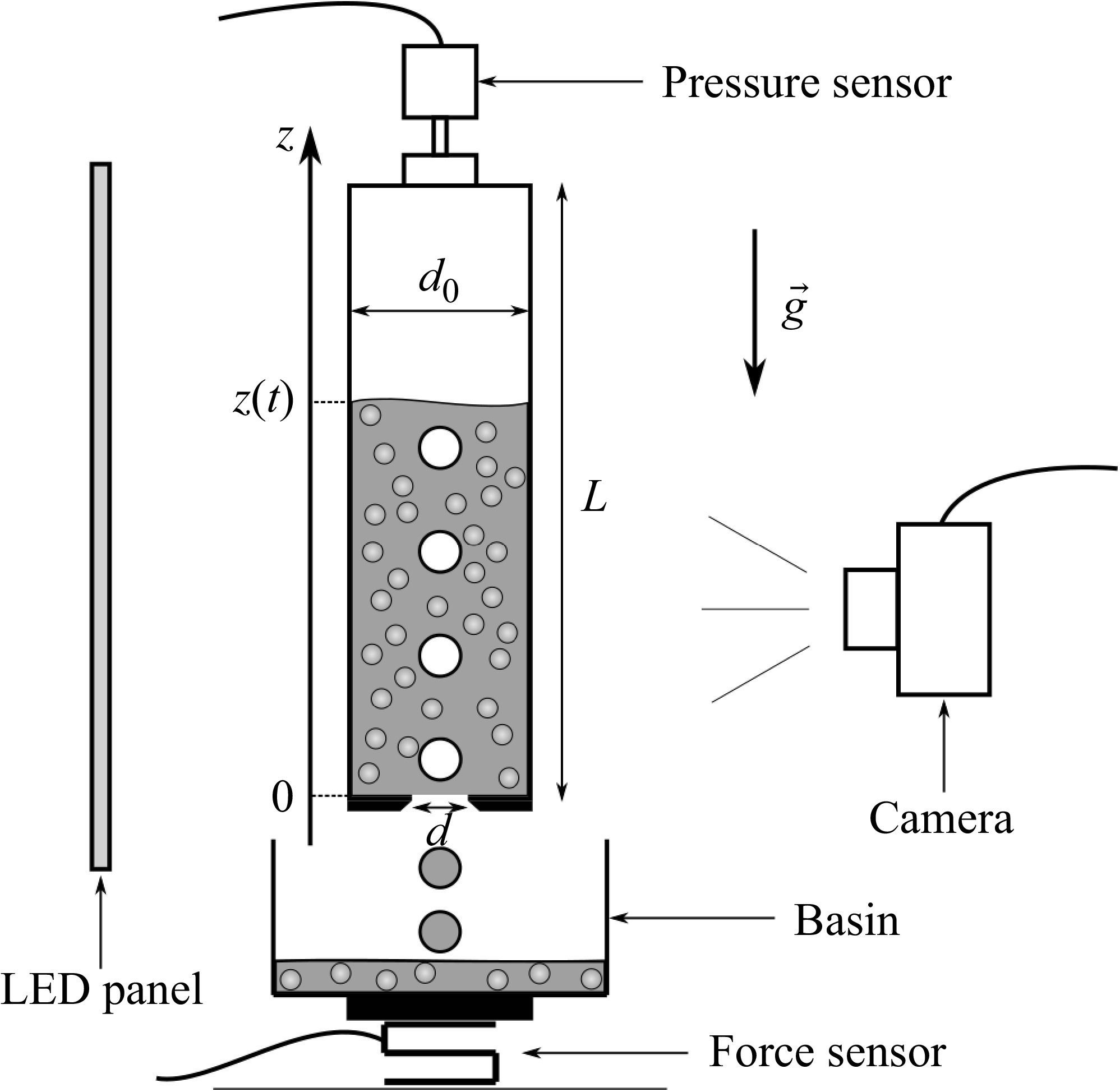


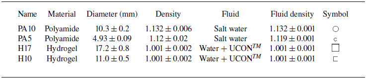


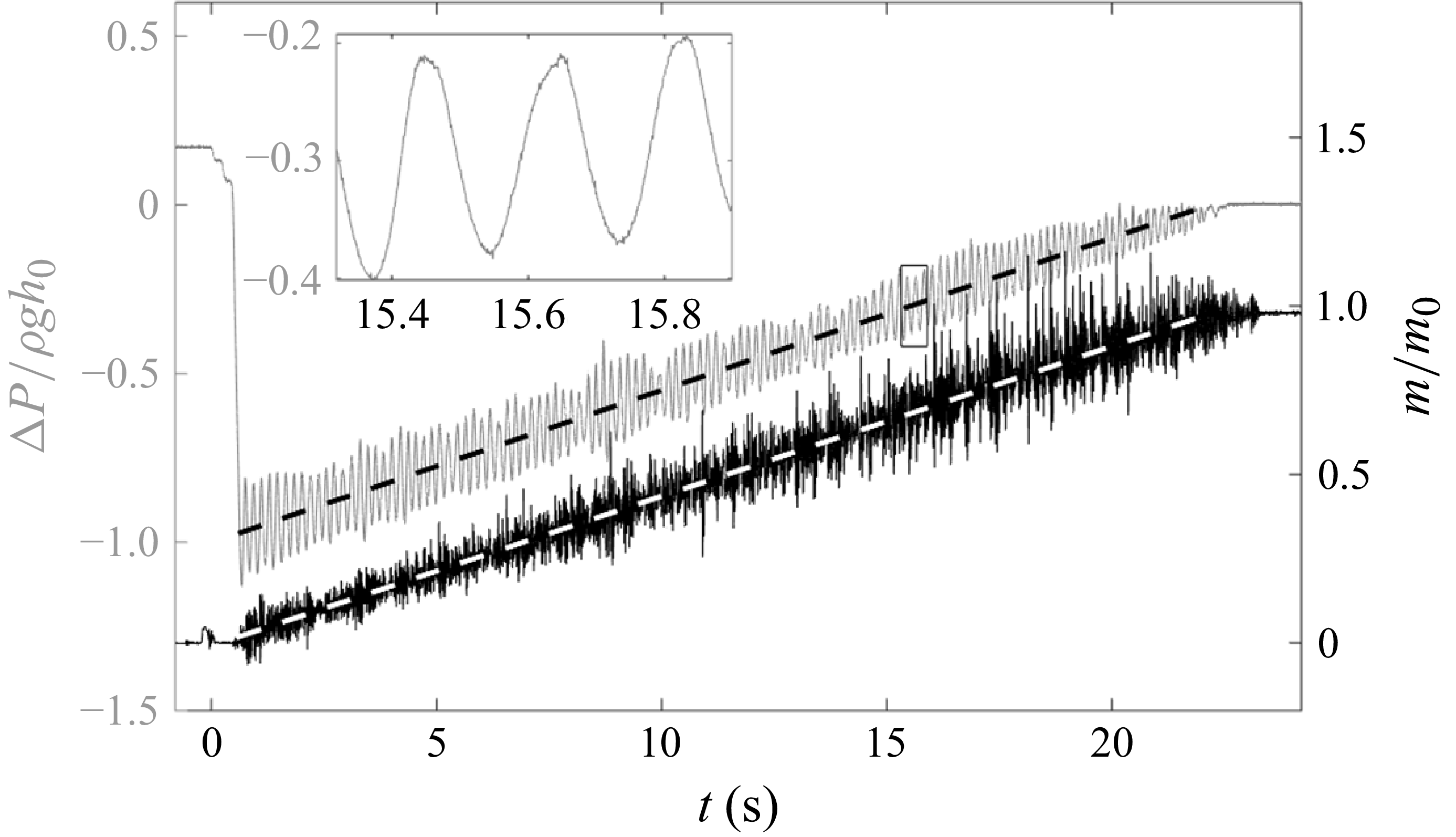


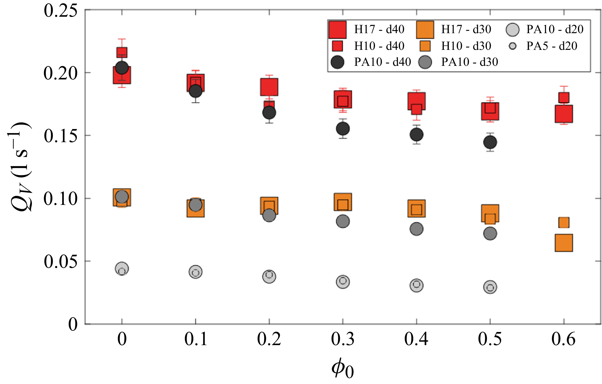


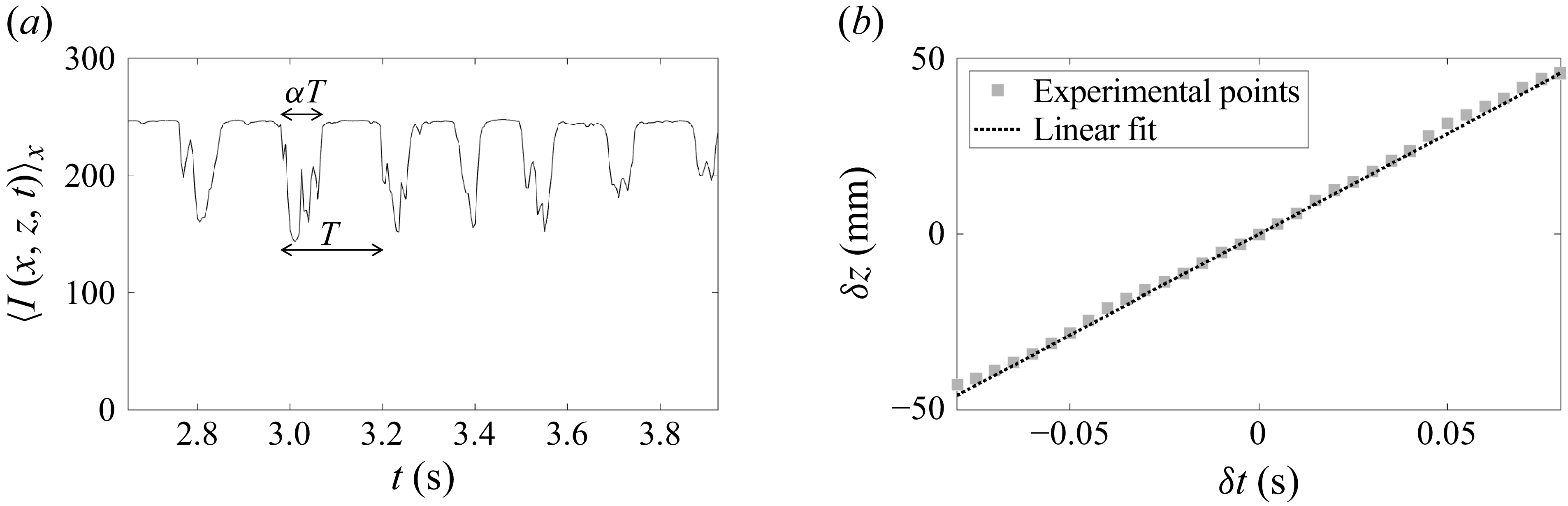


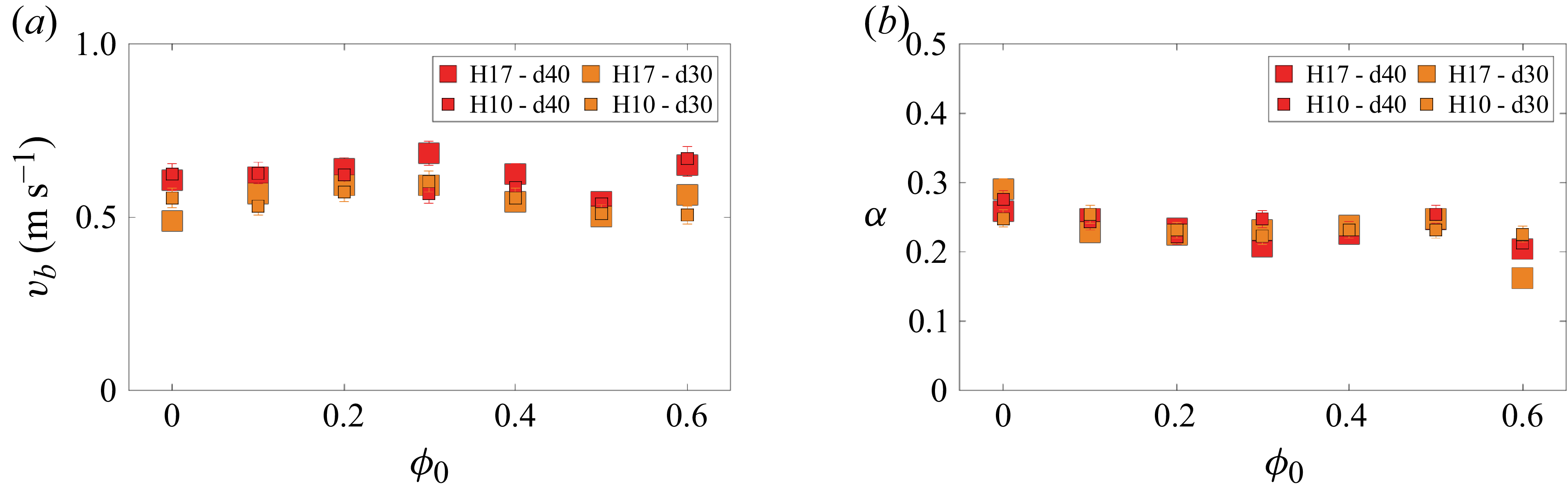


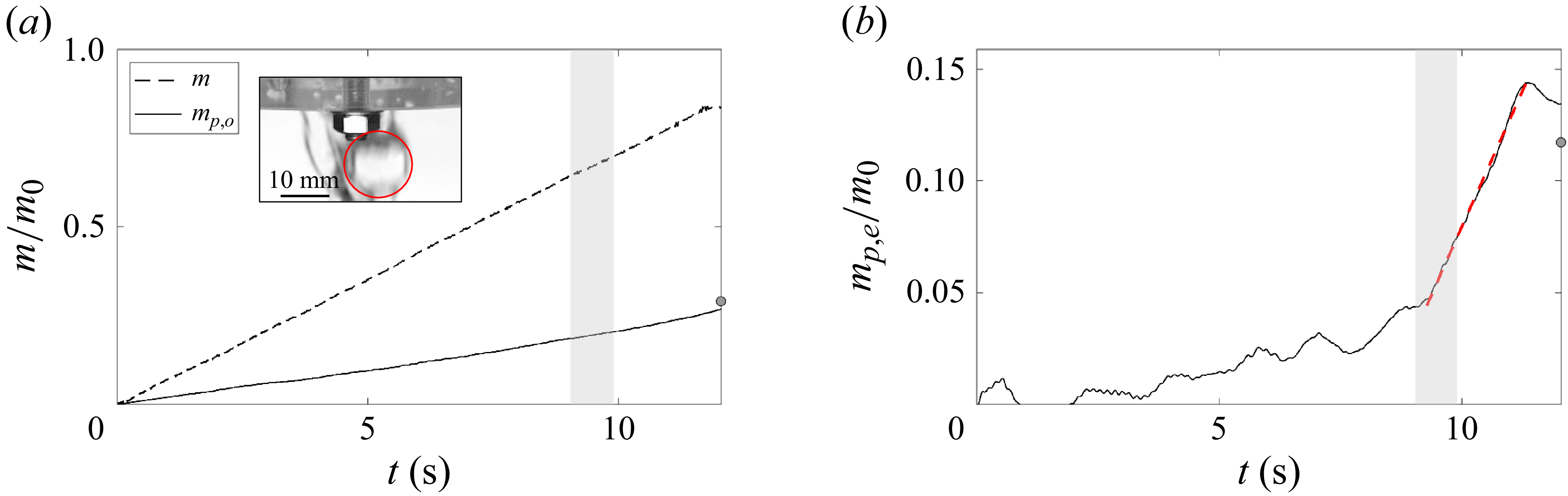


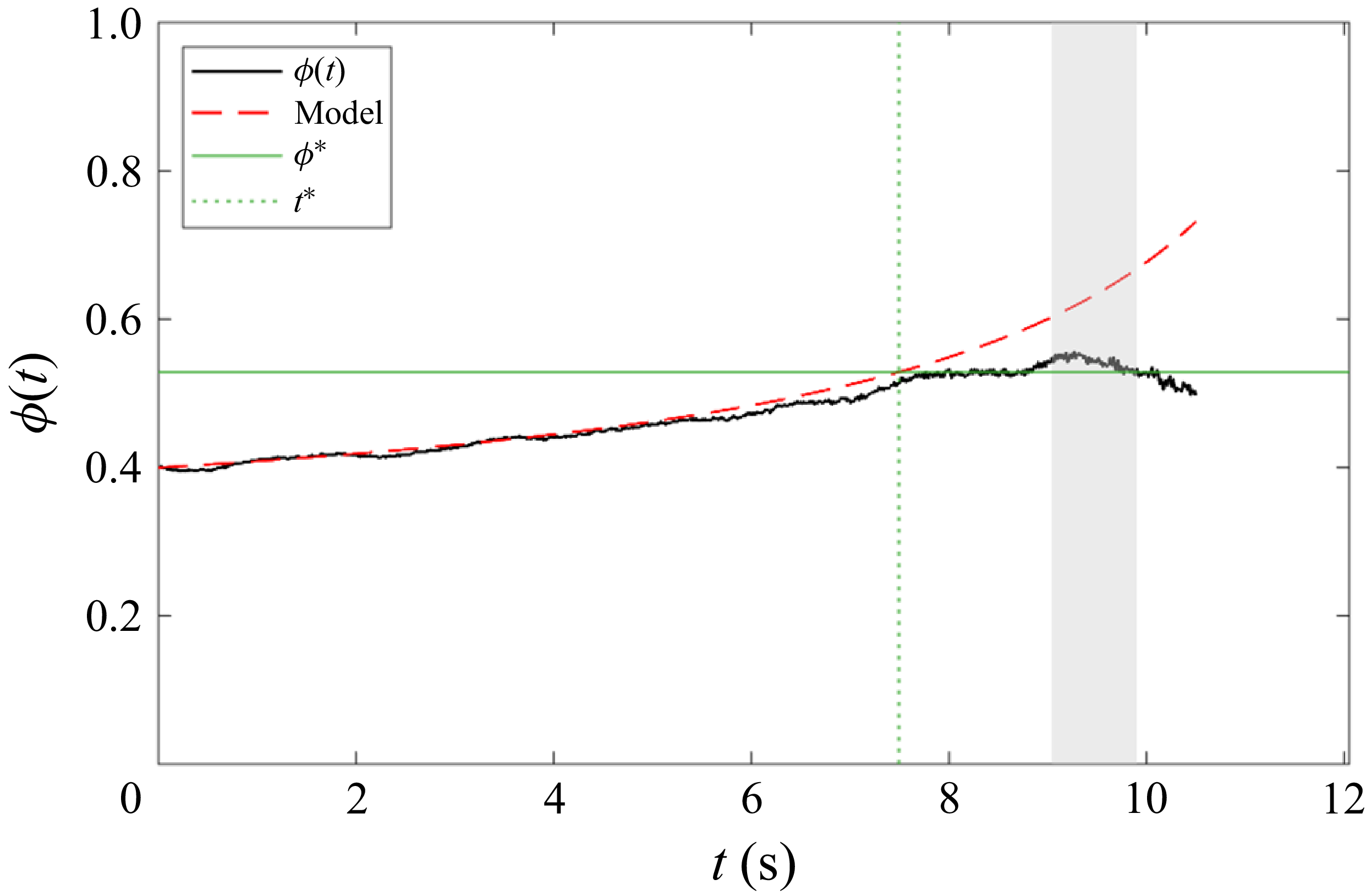


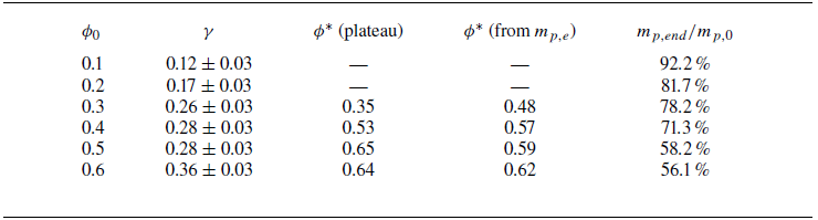


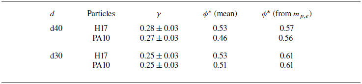


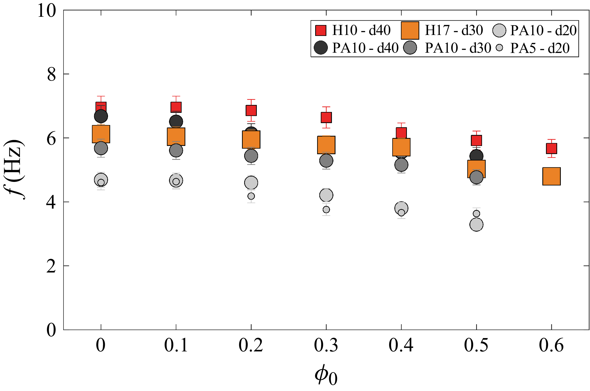


 Open access

