





1. Introduction
Accurate numerical prediction of the true state of a high-speed transitional boundary layer is challenging due to the flow sensitivity to uncertain environmental conditions. Simulations often attempt to address this uncertainty by relying on trial-and-error approaches to model environmental factors through boundary conditions. However, this method is inefficient and can lead to simulations that fail to accurately represent the flow of interest. Data assimilation (DA) provides a rigorous alternative by infusing simulations with experimental measurements. In the present study, an ensemble-variational (EnVar) DA technique is applied to simulate the high-speed flow over a cone–flare geometry, with the assimilated measurements taken from a limited number of high-frequency pressure sensors mounted on the surface near the compression corner (figure 1).
High-speed boundary-layer flows over cone–flare geometries received attention as early as the 1950s, with Becker & Korycinski (Reference Becker and Korycinski1956) reporting a ‘serious heating problem’ attributed to ‘the occurrence of shock–boundary-layer interaction with separation’. This shock–boundary-layer interaction arises as the compression corner generates an adverse pressure gradient, separating the flow and leading to the development of a recirculation bubble together with an oblique shock upstream of separation. The experiments by Chapman, Kuehn & Larson (Reference Chapman, Kuehn and Larson1957), Schaefer & Ferguson (Reference Schaefer and Ferguson1962), Ginoux (Reference Ginoux1965) and Heffner, Chpoun & Lengrand (Reference Heffner, Chpoun and Lengrand1993) also reported an intensification of the thermomechanical surface loading in the presence of a compression corner. Additionally, Ginoux (Reference Ginoux1965) and Heffner et al. (Reference Heffner, Chpoun and Lengrand1993) observed three-dimensional patterns in the form of streaky motions across the reattachment region of the recirculation bubble.
Since the flow on the cone–flare geometry is not parallel and the shock produces nonlinear interactions with the boundary layer, existing theoretical results from simpler configurations provide a partial view only for how disturbances may behave in such situations. Those simpler configurations include, for example, the classical free-stream disturbance–shock interactions (Kovasznay Reference Kovasznay1953; Ribner Reference Ribner1953; McKenzie & Westphal Reference McKenzie and Westphal1968) or parallel and spatial boundary layers without shocks (Mack Reference Mack1975, Reference Mack1984) which are relevant upstream of the compression corner. Numerical studies with high spatio-temporal resolution can provide a window into the dynamics of these flow fields (Pruett & Chang Reference Pruett and Chang1998; Adams Reference Adams, Liu, Sakell and Beutner2001; Lawal & Sandham Reference Lawal and Sandham2001; Pagella, Rist & Wagner Reference Pagella, Rist and Wagner2001; Vandomme et al. Reference Vandomme, Chanetz, Benay and Perraud2003), and have reported intensification of thermomechanical loads across and downstream of the reattachment point of the shear layer on the flare. Pagella et al. (Reference Pagella, Rist and Wagner2001) quantified prediction errors of linear stability analysis based on the parallel flow assumption, and Adams (Reference Adams, Liu, Sakell and Beutner2001) documented stabilisation of the most unstable mode predicted by the linear stability theory of Mack (Reference Mack1984), the second Mack mode, within the recirculation bubble of a Mach 5 boundary layer over a flat plate with a $+15^{\circ }$
compression ramp. Simulations by Balakumar, Zhao & Atkins (Reference Balakumar, Zhao and Atkins2005) for Mach 5.373 flow over a
$+15^{\circ }$
compression ramp. Simulations by Balakumar, Zhao & Atkins (Reference Balakumar, Zhao and Atkins2005) for Mach 5.373 flow over a $+5.5^{\circ }$
compression corner, emulating the Hyper-X model (Berry, DiFulvio & Kowalkowski Reference Berry, DiFulvio and Kowalkowski2000), also revealed that the second Mack mode amplifies prior to separation, stabilises within the recirculation bubble and amplifies again downstream of reattachment. Experiments on axisymmetric geometries with compression corners at different Reynolds and Mach numbers have shown that configurations in which the flow transitions near reattachment can exhibit three to five times the heat transfer of fully turbulent cases, suggesting that triggering transition to turbulence upstream of the separation point might mitigate material loading (Benay et al. Reference Benay, Chanetz, Mangin, Vandomme and Perraud2006; Bur & Chanetz Reference Bur and Chanetz2009; Estruch-Samper et al. Reference Estruch-Samper, Ganapathisubramani, Vanstone and Hillier2012, Reference Estruch-Samper, Vanstone, Ganapathisubramani and Hillier2013; Vanstone et al. Reference Vanstone, Estruch-Samper, Hillier and Ganapathisubramani2013). This highlights the importance of analysing transitional boundary layers.
$+5.5^{\circ }$
compression corner, emulating the Hyper-X model (Berry, DiFulvio & Kowalkowski Reference Berry, DiFulvio and Kowalkowski2000), also revealed that the second Mack mode amplifies prior to separation, stabilises within the recirculation bubble and amplifies again downstream of reattachment. Experiments on axisymmetric geometries with compression corners at different Reynolds and Mach numbers have shown that configurations in which the flow transitions near reattachment can exhibit three to five times the heat transfer of fully turbulent cases, suggesting that triggering transition to turbulence upstream of the separation point might mitigate material loading (Benay et al. Reference Benay, Chanetz, Mangin, Vandomme and Perraud2006; Bur & Chanetz Reference Bur and Chanetz2009; Estruch-Samper et al. Reference Estruch-Samper, Ganapathisubramani, Vanstone and Hillier2012, Reference Estruch-Samper, Vanstone, Ganapathisubramani and Hillier2013; Vanstone et al. Reference Vanstone, Estruch-Samper, Hillier and Ganapathisubramani2013). This highlights the importance of analysing transitional boundary layers.
Flow configuration. (a) Cone–flare geometry, computational domain and sensor locations. (b) Snapshot of the simulated flow. Blue-white-red contours show wall-pressure fluctuations ( $p^{\prime }$
); red iso-surface marks separation identified as by zero streamwise velocity (
$p^{\prime }$
); red iso-surface marks separation identified as by zero streamwise velocity ( $u_{\xi }=0$
); purple iso-surface is the corner shock. (a, b) The axial length is scaled down by a factor of two.
$u_{\xi }=0$
); purple iso-surface is the corner shock. (a, b) The axial length is scaled down by a factor of two.

Figure 1. Long description
The image consists of two parts. Part (a) illustrates the coneflare geometry, computational domain, and sensor locations. The diagram includes labeled axes (x, y, z), angles (theta1, theta2), and points (s1, s2, s3, s4, s5, s6). It also shows the flow direction with arrows labeled M∞ and Me, and coordinates η and ξ. Part (b) presents a snapshot of the simulated flow over the coneflare geometry. It features blue-white-red contours indicating wall-pressure fluctuations, a red iso-surface marking separation identified by zero streamwise velocity, and a purple iso-surface representing the corner shock. The axial length in both parts is scaled down by a factor of two.
Upstream of separation, the disturbance dynamics generally aligns with linear stability theory (Mack Reference Mack1984; Malik & Spall Reference Malik and Spall1991; Kennedy et al. Reference Kennedy, Laurence, Smith and Marineau2018), showing the emergence of the second Mack mode as the most unstable and dominant feature. However, streaky patterns are also observed in numerical simulations of flared or straight cones without compression corners (Laible & Fasel Reference Laible and Fasel2011; Hader & Fasel Reference Hader and Fasel2017, Reference Hader and Fasel2018; Buchta, Laurence & Zaki Reference Buchta, Laurence and Zaki2022; Kennedy et al. Reference Kennedy, Jewell, Paredes and Laurence2022), and can be generated by multiple mechanisms. The streaks can arise within boundary layers from nonlinear interactions of oblique waves (Fasel & Thumm Reference Fasel and Thumm1991; Thumm Reference Thumm1991; Fasel, Thumm & Bestek Reference Fasel, Thumm and Bestek1993) or due to non-modal amplification, as reported by Caillaud et al. (Reference Caillaud2025) for a cone–cylinder–flare configuration at Mach $6$
.
$6$
.
Lugrin et al. (Reference Lugrin, Beneddine, Leclercq, Garnier and Bur2021) performed direct simulations and linear analysis of Mach $5$
flow on a cylinder–flare with a
$5$
flow on a cylinder–flare with a $+15^{\circ }$
compression corner. They underscored the role of oblique modes for the nonlinear amplification of streaks, upstream and within the separation region. Paredes et al. (Reference Paredes, Scholten, Choudhari, Li, Benitez and Jewell2022) performed simulations of a separated cone–cylinder–flare geometry, and showed that oblique convective disturbances experience larger amplification rates than planar disturbances on the separated shear layer: these oblique waves also likely correspond to the shear-layer disturbances observed in the experiments of Benitez et al. (Reference Benitez, Esquieu, Jewell and Schneider2020) and Butler & Laurence (Reference Butler and Laurence2022). The results reveal two scenarios: (i) oblique waves dominate upstream of separation, or (ii) oblique waves emerge after separation as the initially dominant second Mack modes (planar) are dampened and stabilised by the recirculation bubble. Since oblique waves generate streaky structures through nonlinear interactions, these results help to explain the ubiquity of streaky structures in such flows.
$+15^{\circ }$
compression corner. They underscored the role of oblique modes for the nonlinear amplification of streaks, upstream and within the separation region. Paredes et al. (Reference Paredes, Scholten, Choudhari, Li, Benitez and Jewell2022) performed simulations of a separated cone–cylinder–flare geometry, and showed that oblique convective disturbances experience larger amplification rates than planar disturbances on the separated shear layer: these oblique waves also likely correspond to the shear-layer disturbances observed in the experiments of Benitez et al. (Reference Benitez, Esquieu, Jewell and Schneider2020) and Butler & Laurence (Reference Butler and Laurence2022). The results reveal two scenarios: (i) oblique waves dominate upstream of separation, or (ii) oblique waves emerge after separation as the initially dominant second Mack modes (planar) are dampened and stabilised by the recirculation bubble. Since oblique waves generate streaky structures through nonlinear interactions, these results help to explain the ubiquity of streaky structures in such flows.
Numerical simulations and the global linear stability analysis conducted by Sidharth et al. (Reference Sidharth, Dwivedi, Candler and Nichols2018) on a flat plate with a double wedge at Mach 5 identified a critical compression angle beyond which global unstable modes in the form of streaks emerge. That study also concluded that the streaky instability does not originate from centrifugal effects such as Görtler vortices, as had earlier been hypothesised. Esquieu et al. (Reference Esquieu, Benitez, Schneider and Brazier2019) performed linear stability analysis for a cone–cylinder–flare configuration in a Mach 6 boundary layer and compared the results with experiments. Their findings demonstrated that linear computations align with experimental observations to some extent, confirming the presence of linear growth within the recirculation bubble. The input–output linear analysis by Dwivedi et al. (Reference Dwivedi, Sidharth, Nichols, Candler and Jovanović2019) for a Mach-8 boundary-layer flow over a flat plate with a $+15^{\circ }$
compression corner suggests that the amplification of streaks within the recirculation bubble is primarily driven by baroclinic effects. Song & Hao (Reference Song and Hao2025) analysed a Mach 6 boundary layer over a flat plate with different compression corners. They noted that the amplification of streaky structures and oblique waves in the separated region follow similar trends, and suggested a correlation with curvature and a possible role of the Görtler mechanism at separation and reattachment.
$+15^{\circ }$
compression corner suggests that the amplification of streaks within the recirculation bubble is primarily driven by baroclinic effects. Song & Hao (Reference Song and Hao2025) analysed a Mach 6 boundary layer over a flat plate with different compression corners. They noted that the amplification of streaky structures and oblique waves in the separated region follow similar trends, and suggested a correlation with curvature and a possible role of the Görtler mechanism at separation and reattachment.
The experiments by Butler & Laurence (Reference Butler and Laurence2021, Reference Butler and Laurence2022) on a Mach-6 boundary layer over a cone–flare geometry captured a number of interesting physical phenomena, such as the rapid growth of shear-layer disturbances within the separated region that could undergo spontaneous radiation of energy, and the propagation of second-mode disturbance energy along the separation and reattachment shocks. In the quiet-tunnel experiments of Benitez et al. (Reference Benitez, Borg, Scholten, Paredes, McDaniel and Jewell2023), similar shear-layer disturbances were found to break down into turbulent spots within the reattached boundary layer. Complementing these latter experimental findings, the linear stability analysis by Paredes et al. (Reference Paredes, Scholten, Choudhari, Li, Benitez and Jewell2022) on the same cone–cylinder–flare geometry identified global unstable modes in the form of streaky structures as the most unstable features within the recirculation bubble of the axisymmetric geometry, but could not capture the full nonlinear dynamics behind the experimental data used for comparison. These results further reinforce the value of a quantitative approach to interpret limited experimental measurements, which we achieve using DA.
Data assimilation combines experiments and simulations to enable the prediction of flow fields beyond the scope of direct measurements (Zaki Reference Zaki2025). Given experimental data, DA involves solving the inverse problem of determining the input parameters for simulations in order to reproduce the measurements. This approach allows the retrieval of the flow state corresponding to the experimental data, providing non-intrusive access to all flow quantities. Numerous DA strategies have been developed and applied in fluid dynamics, including filtering and nudging (Clark Di Leoni, Mazzino & Biferale Reference Clark Di Leoni, Mazzino and Biferale2020; Wang & Zaki Reference Wang and Zaki2022), adjoint- and ensemble-variational methods (Mons, Wang & Zaki Reference Mons, Wang and Zaki2019; Zaki & Wang Reference Zaki and Wang2021; Wang, Wang & Zaki Reference Wang, Wang and Zaki2022) and neural networks (Buzzicotti et al. Reference Buzzicotti, Bonaccorso, Di Leoni and Biferale2021; Clark Di Leoni et al. Reference Clark Di Leoni, Lu, Meneveau, Karniadakis and Zaki2023; Hao et al. Reference Hao, Clark Di Leoni, Marxen, Meneveau, Karniadakis and Zaki2023; Morra, Meneveau & Zaki Reference Morra, Meneveau and Zaki2024). For example, using wall-pressure measurements, Buchta et al. (Reference Buchta, Laurence and Zaki2022) successfully applied an EnVar technique to compute the energy spectral makeup of incoming external disturbances in a Mach-6 boundary layer over a cone. Their analysis enhanced the accuracy of interpreting sensor data within the nonlinear, transitional flow regime.
Using experimental wall-pressure measurements from flow over a cone–flare geometry (specifically, those from Butler & Laurence Reference Butler and Laurence2022), the present work aims to estimate the upstream boundary-layer disturbances that reproduce the sensor data. The energy spectra of the oncoming disturbances are identified, enabling a full simulation of the flow field. This approach leverages the relationship between wall-pressure observations and the upstream flow (Wang & Zaki Reference Wang and Zaki2025), and yields a reconstructed flow field that surpasses the resolution of the measurements and permits a deeper analysis of the flow phenomena. The importance of sensors within separation for accurate estimation of the upstream flow is highlighted, followed by a detailed analysis of the disturbance fields in the attached boundary layer and across the separation shock. The influence of the unsteady shock–boundary-layer interaction on the uncertainty of the estimation is also examined.
The original experimental configuration and the computational set-up are introduced in § 2. The experimental measurements and the EnVar DA algorithm are presented in § 3, along with the optimisation protocol. The DA solutions with partial observations and with all the sensor data are presented in §§ 4.1 and 4.2. The disturbance dynamics across the shock–boundary-layer interaction, onset of separation and in the reattached flow are the subjects of §§ 4.3 and 4.4, and conclusions are provided in § 5.
2. Flow configuration
2.1. Experimental parameters
The present study focuses on the assimilation of available experimental measurements of high-speed flow over a cone–flare in direct numerical simulations. While the focus is on the assimilation task and the results from the simulations, we include a brief description of the relevant experimental parameters for completeness (for details, see Butler & Laurence Reference Butler and Laurence2022).
The experiment was conducted in the HyperTERP reflected-shock tunnel at the University of Maryland (Butler & Laurence Reference Butler and Laurence2019, Reference Butler and Laurence2021). The facility consists of a reflected-shock tube to generate the effective stagnation conditions, a converging–diverging nozzle to accelerate the flow to hypersonic Mach numbers, a test section where the test article is housed and a dump tank. Table 1 reports the free-stream fluid properties upstream of the test article, including the free-stream density $\rho _{\infty }$
, pressure
$\rho _{\infty }$
, pressure $p_{\infty }$
, temperature
$p_{\infty }$
, temperature $\varTheta _{\infty }$
, speed of sound
$\varTheta _{\infty }$
, speed of sound $a_{\infty }$
, velocity
$a_{\infty }$
, velocity $U_{\infty }$
, Mach number
$U_{\infty }$
, Mach number $M_{\infty }= U_{\infty }/a_{\infty }$
, dynamic shear viscosity
$M_{\infty }= U_{\infty }/a_{\infty }$
, dynamic shear viscosity $\mu _{\infty }=\mu _{\scriptscriptstyle \varTheta =100\textrm{K}}(\varTheta _{\infty } / 100\,\textrm{K})^{0.8497}$
and unit Reynolds number
$\mu _{\infty }=\mu _{\scriptscriptstyle \varTheta =100\textrm{K}}(\varTheta _{\infty } / 100\,\textrm{K})^{0.8497}$
and unit Reynolds number $Re_{\infty }/L = \rho _{\infty }U_{\infty }/\mu _{\infty }$
, where
$Re_{\infty }/L = \rho _{\infty }U_{\infty }/\mu _{\infty }$
, where $L$
is a reference length. The exponent
$L$
is a reference length. The exponent $0.8497$
for the shear viscosity as function of temperature results from fitting the power law to experimental data from Touloukian, Saxena & Hestermans (Reference Touloukian, Saxena and Hestermans1975), with
$0.8497$
for the shear viscosity as function of temperature results from fitting the power law to experimental data from Touloukian, Saxena & Hestermans (Reference Touloukian, Saxena and Hestermans1975), with $\mu _{\scriptscriptstyle \varTheta =100\textrm{K}} = 7.06\times 10^{-6}\,\textrm{kg}\boldsymbol{\cdot}\textrm{s m}^{-1}$
being the viscosity at
$\mu _{\scriptscriptstyle \varTheta =100\textrm{K}} = 7.06\times 10^{-6}\,\textrm{kg}\boldsymbol{\cdot}\textrm{s m}^{-1}$
being the viscosity at $100\,\textrm{K}$
. The table also reports the corresponding stagnation density
$100\,\textrm{K}$
. The table also reports the corresponding stagnation density $\rho _{0}$
, pressure
$\rho _{0}$
, pressure $p_{0}$
, temperature
$p_{0}$
, temperature $\varTheta _{0}$
and speed of sound
$\varTheta _{0}$
and speed of sound $a_{0}$
.
$a_{0}$
.
Stagnation and free-stream tunnel conditions (§ 2.1), and boundary-layer-edge conditions at $x=29.86\,\textrm{cm}$
from the cone nose tip (§ 2.2). Stagnation, free-stream and edge conditions are denoted with subscripts
$x=29.86\,\textrm{cm}$
from the cone nose tip (§ 2.2). Stagnation, free-stream and edge conditions are denoted with subscripts $\{0, \infty , e\}$
.
$\{0, \infty , e\}$
.

Table 1. Long description
The table presents data on stagnation, free-stream, and boundary-layer-edge conditions from a hypersonic wind tunnel experiment. It includes measurements of density, pressure, temperature, velocity, Mach number, dynamic shear viscosity, and unit Reynolds number. The stagnation conditions are denoted with subscript 0, free-stream conditions with subscript infinity, and edge conditions with subscript e. The table lists specific values for each condition, such as a stagnation density of 5.28 kilograms per cubic meter and a free-stream velocity of 1253 meters per second. The data highlights the variations in fluid properties under different experimental conditions.
The test article is a cone–flare geometry with a $10^{\circ }$
compression corner, and is shown schematically in figure 1. The cone has a circular cross-section, a sharp nose with
$10^{\circ }$
compression corner, and is shown schematically in figure 1. The cone has a circular cross-section, a sharp nose with $0.01\,\textrm{cm}$
tip radius, a
$0.01\,\textrm{cm}$
tip radius, a $5^{\circ }$
half-angle and a
$5^{\circ }$
half-angle and a $41.00\,\textrm{cm}$
length. The flare is a circular frustum with a
$41.00\,\textrm{cm}$
length. The flare is a circular frustum with a $15^{\circ }$
half-angle and a
$15^{\circ }$
half-angle and a $7.62\,\textrm{cm}$
length. Throughout, lengths are measured along the axis of revolution from the nose unless otherwise specified. The test article is oriented at a zero angle of incidence with respect to the streamwise direction. The model is at room temperature (
$7.62\,\textrm{cm}$
length. Throughout, lengths are measured along the axis of revolution from the nose unless otherwise specified. The test article is oriented at a zero angle of incidence with respect to the streamwise direction. The model is at room temperature ( $\varTheta _{w}=300\,\textrm{K}$
) before the flow is accelerated to hypersonic conditions. The test time (
$\varTheta _{w}=300\,\textrm{K}$
) before the flow is accelerated to hypersonic conditions. The test time ( $6\,\textrm{ms}$
) is sufficiently brief that changes in the surface temperature can be neglected. Nine PCB 132B38 pressure transducers are flush-mounted on the surface of the cone–flare, following the line of the axis of revolution. The DA considered the first seven sensors, which comprise all four sensors on the cone, designated
$6\,\textrm{ms}$
) is sufficiently brief that changes in the surface temperature can be neglected. Nine PCB 132B38 pressure transducers are flush-mounted on the surface of the cone–flare, following the line of the axis of revolution. The DA considered the first seven sensors, which comprise all four sensors on the cone, designated $s_1$
through
$s_1$
through $s_4$
, and the first three sensors on the flare,
$s_4$
, and the first three sensors on the flare, $s_5$
through
$s_5$
through $s_7$
. The downstream positions of these sensors along the cone axis are listed in table 2. Sensors downstream of
$s_7$
. The downstream positions of these sensors along the cone axis are listed in table 2. Sensors downstream of $s_7$
are excluded, as we focus on the region upstream of turbulence where the dynamics is transitional and dominated by unsteady disturbances interacting with the boundary layer, shocks and the recirculation bubble. Data from sensor
$s_7$
are excluded, as we focus on the region upstream of turbulence where the dynamics is transitional and dominated by unsteady disturbances interacting with the boundary layer, shocks and the recirculation bubble. Data from sensor $s_8$
will, however, be used for independent comparison with the results from the assimilation of the data from the preceding seven sensors. A description of the experimental measurements used for DA is provided in § 3.1.
$s_8$
will, however, be used for independent comparison with the results from the assimilation of the data from the preceding seven sensors. A description of the experimental measurements used for DA is provided in § 3.1.
Sensor locations along the $x$
-axis. Sensor
$x$
-axis. Sensor $s_8$
data are not assimilated, and will be used for independent validation.
$s_8$
data are not assimilated, and will be used for independent validation.

Table 2. Long description
The table presents the locations of eight sensors along the x-axis, measured in centimeters. The sensors are labeled s1 through s8, with their respective locations listed as follows: s1 at 32.48 centimeters, s2 at 35.17 centimeters, s3 at 37.96 centimeters, s4 at 39.75 centimeters, s5 at 41.33 centimeters, s6 at 42.03 centimeters, s7 at 43.17 centimeters, and s8 at 44.42 centimeters. The table is structured with two columns: one for the sensor labels and one for their corresponding locations.
2.2. Computational set-up
The DA requires a computational model, which in the present study is direct numerical simulation of the compressible Navier–Stokes equations. The simulation domain is the sub-volume marked in figure 1, downstream of the conical shock which has an angle $\theta _s = 10.64^{\circ }$
. The edge conditions are determined using the free-stream experimental values from § 2.1, the thermodynamic relations across the leading shock and the Taylor–Maccoll approximation for inviscid axisymmetric flow above the boundary layer of a cone (Stewartson Reference Stewartson1964; Malik & Spall Reference Malik and Spall1991). The edge conditions are summarised in table 1.
$\theta _s = 10.64^{\circ }$
. The edge conditions are determined using the free-stream experimental values from § 2.1, the thermodynamic relations across the leading shock and the Taylor–Maccoll approximation for inviscid axisymmetric flow above the boundary layer of a cone (Stewartson Reference Stewartson1964; Malik & Spall Reference Malik and Spall1991). The edge conditions are summarised in table 1.
Two coordinate systems will be adopted where convenient: Cartesian coordinates $(x, y, z)$
and curvilinear body-fitted coordinates
$(x, y, z)$
and curvilinear body-fitted coordinates $(\xi , \eta , \vartheta )$
, in a reference frame centred at the nose tip of the cone–flare. In the Cartesian frame, which is marked in figure 1, the cone–flare axis of revolution lies along the
$(\xi , \eta , \vartheta )$
, in a reference frame centred at the nose tip of the cone–flare. In the Cartesian frame, which is marked in figure 1, the cone–flare axis of revolution lies along the $x$
-axis, the
$x$
-axis, the $xy$
-plane contains both the axis of revolution and the sensors and the
$xy$
-plane contains both the axis of revolution and the sensors and the $z$
-axis is perpendicular to the
$z$
-axis is perpendicular to the $xy$
-plane. In the curvilinear frame of reference, the
$xy$
-plane. In the curvilinear frame of reference, the $\xi$
-axis runs parallel to the cone–flare wall, the
$\xi$
-axis runs parallel to the cone–flare wall, the $\eta$
-axis is normal to the cone wall and the
$\eta$
-axis is normal to the cone wall and the $\vartheta$
-axis is perpendicular to the
$\vartheta$
-axis is perpendicular to the $\xi \eta$
-plane.
$\xi \eta$
-plane.
The fluid is assumed to be a calorically perfect gas with a ratio of specific heats $\gamma = C_p/C_v = 1.4$
. The flow is governed by the dimensional Navier–Stokes equations
$\gamma = C_p/C_v = 1.4$
. The flow is governed by the dimensional Navier–Stokes equations
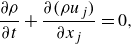 \begin{align} \frac {\partial \rho }{\partial t} + \frac {\partial (\rho u_j)}{\partial x_j} &= 0, \end{align}
 \begin{align} \frac {\partial (\rho u_i)}{\partial t} + \frac {\partial }{\partial x_j}(\rho u_i u_j) &= - \frac {\partial p}{\partial x_i} + \frac {\partial \tau _{ij}}{\partial x_j}, \end{align}
 \begin{align} \frac {\partial E}{\partial t} + \frac {\partial }{\partial x_j} \big[u_j(E+p)\big] &= \frac {\partial }{\partial x_j} (u_i \tau _{ij}) + \frac {\partial }{\partial x_j} \left ( \kappa \frac {\partial \varTheta }{\partial x_j}\right ), \end{align}
where $u_i$
is the ith velocity component (
$u_i$
is the ith velocity component ( $i=1,2,3$
),
$i=1,2,3$
), $E = p/(\gamma - 1) + 0.5 \rho u_i u_i$
is the total energy and
$E = p/(\gamma - 1) + 0.5 \rho u_i u_i$
is the total energy and $\varTheta = p / ( R\rho )$
is the temperature, with gas constant
$\varTheta = p / ( R\rho )$
is the temperature, with gas constant $R=287\,\textrm{J \, (kg\,K)}^{-1}$
. Thermal conductivity is given by
$R=287\,\textrm{J \, (kg\,K)}^{-1}$
. Thermal conductivity is given by $\kappa =\mu C_p /Pr$
. The dynamic shear viscosity is modelled as
$\kappa =\mu C_p /Pr$
. The dynamic shear viscosity is modelled as $\mu =\mu _e (\varTheta /\varTheta _e)^{0.8497}$
, while the Prandtl number
$\mu =\mu _e (\varTheta /\varTheta _e)^{0.8497}$
, while the Prandtl number $Pr=0.72$
is assumed constant, consistent with ideal gas behaviour (Touloukian et al. Reference Touloukian, Saxena and Hestermans1975). The viscous stress tensor
$Pr=0.72$
is assumed constant, consistent with ideal gas behaviour (Touloukian et al. Reference Touloukian, Saxena and Hestermans1975). The viscous stress tensor $\tau _{ij}$
is given by
$\tau _{ij}$
is given by
 \begin{align} \tau _{ij} = \mu \left ( \frac {\partial u_i}{\partial x_j} + \frac {\partial u_j}{\partial x_i} \right ) + \left ( \mu _b-\frac {2}{3}\mu \right ) \delta _{ij} \frac {\partial u_k}{\partial x_k}. \end{align}
The governing equations (2.1–2.4) can be expressed in compact form as $\boldsymbol{q} = {\mathcal{N}}(\boldsymbol{c})$
, where
$\boldsymbol{q} = {\mathcal{N}}(\boldsymbol{c})$
, where $\boldsymbol{q} = [\rho , \rho u_1, \rho u_2, \rho u_3, E]^{\top }$
is the state vector,
$\boldsymbol{q} = [\rho , \rho u_1, \rho u_2, \rho u_3, E]^{\top }$
is the state vector, ${\mathcal{N}}$
is the Navier–Stokes operator and
${\mathcal{N}}$
is the Navier–Stokes operator and $\boldsymbol{c}$
is the vector of control parameters which we must accurately estimate in order to reproduce the experimental data. In the present study,
$\boldsymbol{c}$
is the vector of control parameters which we must accurately estimate in order to reproduce the experimental data. In the present study, $\boldsymbol{c}$
will comprise the oncoming boundary-layer disturbance spectra, at the inflow to the computational domain.
$\boldsymbol{c}$
will comprise the oncoming boundary-layer disturbance spectra, at the inflow to the computational domain.
The start of the computational domain on the cone surface is at $x_0 = 29.86\,\textrm{cm}$
(
$x_0 = 29.86\,\textrm{cm}$
( $\xi _{0} = 30.00\,\textrm{cm}$
), and the vertical extent is from the cone surface
$\xi _{0} = 30.00\,\textrm{cm}$
), and the vertical extent is from the cone surface $\eta _0$
to
$\eta _0$
to $\eta _{max} = 2.55\,\textrm{cm}$
. The azimuthal domain size is
$\eta _{max} = 2.55\,\textrm{cm}$
. The azimuthal domain size is $36^{\circ }$
, which can accommodate linearly unstable three-dimensional modes and, as will be shown, is sufficiently large to capture the steady streaks in the assimilated flow. The domain consists of a swept volume, where the inlet surface is translated along the cone–flare (
$36^{\circ }$
, which can accommodate linearly unstable three-dimensional modes and, as will be shown, is sufficiently large to capture the steady streaks in the assimilated flow. The domain consists of a swept volume, where the inlet surface is translated along the cone–flare ( $\xi$
-axis) to the outlet. The downstream edge of the computational domain, on the cone surface, is
$\xi$
-axis) to the outlet. The downstream edge of the computational domain, on the cone surface, is $x_{max} = 44.56\,\textrm{cm}$
. On the cone surface, no-slip and isothermal conditions are imposed, with the wall temperature fixed at
$x_{max} = 44.56\,\textrm{cm}$
. On the cone surface, no-slip and isothermal conditions are imposed, with the wall temperature fixed at $\varTheta _{w} = 300\,\text{K}$
as in the experiment. Periodic boundary conditions are applied in the azimuthal direction. A sponge region is included at the top (
$\varTheta _{w} = 300\,\text{K}$
as in the experiment. Periodic boundary conditions are applied in the azimuthal direction. A sponge region is included at the top ( $\varDelta \eta _{sponge} = 6.54\,\textrm{mm}$
) and outlet (
$\varDelta \eta _{sponge} = 6.54\,\textrm{mm}$
) and outlet ( $\varDelta \xi _{sponge} = 0.8\,\textrm{mm}$
), where a forcing term dampens the fluctuations and drives the flow towards a reference laminar solution
$\varDelta \xi _{sponge} = 0.8\,\textrm{mm}$
), where a forcing term dampens the fluctuations and drives the flow towards a reference laminar solution $\boldsymbol{q}_{\scriptscriptstyle B}$
. The laminar state is shown in figure 2, and exhibits key features including the recirculation bubble and the separation and reattachment shocks.
$\boldsymbol{q}_{\scriptscriptstyle B}$
. The laminar state is shown in figure 2, and exhibits key features including the recirculation bubble and the separation and reattachment shocks.
Contours of pressure in the axisymmetric undisturbed flow, $\boldsymbol{q}_{\scriptscriptstyle B}$
. (
$\boldsymbol{q}_{\scriptscriptstyle B}$
. (
 ) The boundary-layer thickness $\delta _{\scriptscriptstyle 99}$
; (
$\delta _{\scriptscriptstyle 99}$
; (
 ) separation and reattachment shocks; (
 ) velocity streamlines; (
 ) sonic line; (
 , white) recirculation bubble identified by $u_{\xi ,{\scriptscriptstyle B}} =0$
; (
$u_{\xi ,{\scriptscriptstyle B}} =0$
; ( $s_{1}$
–
$s_{1}$
– $s_{7}$
) sensor locations.
$s_{7}$
) sensor locations.

Figure 2. Long description
A heat map illustrates pressure contours in an axisymmetric undisturbed flow. The map features a color gradient indicating pressure levels, with lighter colors representing higher pressure values and darker colors indicating lower pressure values. The x-axis ranges from 30 to 44 centimeters, and the y-axis ranges from 3.0 to 4.5 centimeters. The boundary-layer thickness is marked with blue lines, while separation and reattachment shocks are highlighted with black dashed lines. Velocity streamlines are depicted with black lines, and the sonic line is shown with a black solid line. The recirculation bubble is identified by a white contour. Seven sensor locations are marked with black dots labeled S1 through S7. The heat map reveals a gradient of pressure increasing from left to right, with notable features such as the boundary-layer thickness, separation and reattachment shocks, and the recirculation bubble. The sensor locations are strategically placed to capture data across the flow field.
In order to reproduce the experimental measurements, disturbances are introduced at the inlet plane, $\boldsymbol{x} = \boldsymbol{x}_{in}$
, superposed onto the laminar base flow,
$\boldsymbol{x} = \boldsymbol{x}_{in}$
, superposed onto the laminar base flow, $\boldsymbol{q} = \boldsymbol{q}_{\scriptscriptstyle B}(\boldsymbol{x}_{in}) + \boldsymbol{q}^{\prime }_{\scriptscriptstyle {\mathcal{L}}}(\boldsymbol{x}_{in},t)$
. Subscript
$\boldsymbol{q} = \boldsymbol{q}_{\scriptscriptstyle B}(\boldsymbol{x}_{in}) + \boldsymbol{q}^{\prime }_{\scriptscriptstyle {\mathcal{L}}}(\boldsymbol{x}_{in},t)$
. Subscript ${\mathcal{L}}$
indicates that these disturbances are computed using linear theory. Specifically, the disturbances are harmonic in time with frequency
${\mathcal{L}}$
indicates that these disturbances are computed using linear theory. Specifically, the disturbances are harmonic in time with frequency $f_n$
and in the span with wavenumber
$f_n$
and in the span with wavenumber $k_m$
; for each
$k_m$
; for each $ (f_n,k_m )$
pair, the wall-normal profile corresponds to the most unstable discrete eigenfunction
$ (f_n,k_m )$
pair, the wall-normal profile corresponds to the most unstable discrete eigenfunction $\boldsymbol{\breve {q}}_{n,m}$
of the spatial linear stability operator
$\boldsymbol{\breve {q}}_{n,m}$
of the spatial linear stability operator
 \begin{align} \boldsymbol{q}^{\prime }_{\scriptscriptstyle {\mathcal{L}}}(\boldsymbol{x}_{in}, t) = \sum _{n,m} \frac {c_{n,m}}{\sqrt {2}} \textrm{Re}\! \left [ {\boldsymbol{\breve {q}}_{n,m}} e^{i (k_{m} \vartheta - 2\pi f_{n} t + \psi _{n,m}) } \right ]. \end{align}
Since equation (2.5) is evaluated at the inflow, the streamwise exponential $e^{i \alpha _{m,n} \xi _{in}}$
is constant and is absorbed in the amplitude and phase for every mode. Parameterisation of the inflow disturbances using the eigenfunctions
$e^{i \alpha _{m,n} \xi _{in}}$
is constant and is absorbed in the amplitude and phase for every mode. Parameterisation of the inflow disturbances using the eigenfunctions $\boldsymbol{\breve {q}}_{n,m}$
from linear stability theory is motivated by the prominence of the associated frequencies in the experimental wall-pressure spectra at the upstream-most sensors, as will be seen in § 3.1. The eigenfunctions are normalised to unit energy
$\boldsymbol{\breve {q}}_{n,m}$
from linear stability theory is motivated by the prominence of the associated frequencies in the experimental wall-pressure spectra at the upstream-most sensors, as will be seen in § 3.1. The eigenfunctions are normalised to unit energy
 \begin{align} \frac {1}{2\rho _{e}U_{e}^2\delta _e} \int _{\eta _0}^{\eta _{max}} \left [ \rho _{\scriptscriptstyle B} |\breve {u}_{i}|^2 + R\,\frac {\varTheta _{\scriptscriptstyle B}}{\rho _{\scriptscriptstyle B}} |\, \breve {\rho } |^2 + \frac {R}{\gamma -1} \frac {\rho _{\scriptscriptstyle B}}{\varTheta _{\scriptscriptstyle B}} | \breve {\varTheta } |^2 \right ] \ {\textrm{d}}\eta = 1, \quad \quad i = 1,2,3, \end{align}
using the norm by Chu (Reference Chu1965), where $\delta _e$
is the Mangler-transformed Blasius length scale at the inflow.
$\delta _e$
is the Mangler-transformed Blasius length scale at the inflow.
The prescribed inflow frequencies are $f_n \in \{50,\, 55, \ldots , 350\}\,\textrm{kHz}$
with
$f_n \in \{50,\, 55, \ldots , 350\}\,\textrm{kHz}$
with $n = 1,2,\ldots ,N_{f}$
and
$n = 1,2,\ldots ,N_{f}$
and $N_{f} = 61$
, while the prescribed azimuthal wavenumbers are
$N_{f} = 61$
, while the prescribed azimuthal wavenumbers are $k_m \in \{0,20,30,40\}$
with
$k_m \in \{0,20,30,40\}$
with $m = 1,\ldots ,N_k$
and
$m = 1,\ldots ,N_k$
and $N_k = 4$
. These ranges were identified based on spectral analysis of the measurements (§ 3.1), and encompass Mack’s first and second modes at the inlet plane. In figure 3(
$N_k = 4$
. These ranges were identified based on spectral analysis of the measurements (§ 3.1), and encompass Mack’s first and second modes at the inlet plane. In figure 3( $a$
), we plot the local spatial growth rates
$a$
), we plot the local spatial growth rates $\alpha _r$
of these discrete modes, over an expanded range of frequencies. The eigenfunction associated with the peak growth rate is then reported in figure 3(
$\alpha _r$
of these discrete modes, over an expanded range of frequencies. The eigenfunction associated with the peak growth rate is then reported in figure 3( $b$
). As expected for modes in the discrete branch,
$b$
). As expected for modes in the discrete branch, $\breve {\boldsymbol{q}}_{n,m}(\eta )$
is contained within the boundary layer. Using the linearised Navier–Stokes equations, the inflow modes were evolved along the early portion of the cone and their
$\breve {\boldsymbol{q}}_{n,m}(\eta )$
is contained within the boundary layer. Using the linearised Navier–Stokes equations, the inflow modes were evolved along the early portion of the cone and their $N$
-factors are reported in figure 3(
$N$
-factors are reported in figure 3( $c$
). The results demonstrate that the planar and oblique waves with frequencies
$c$
). The results demonstrate that the planar and oblique waves with frequencies $f_n \in [225,310]\,\textrm{kHz}$
are the linearly most amplified downstream. The DA then exploits the amplification and nonlinear interactions among the inflow modes to match the experimental measurements, for example for the generation of higher harmonics of the inlet frequencies or the formation of streaky structures (Novikov, Egorov & Fedorov Reference Novikov, Egorov and Fedorov2016). The linearly stable lower frequencies are also included at the inlet due to their relevance in the separated region, which can destabilise these waves. The phases
$f_n \in [225,310]\,\textrm{kHz}$
are the linearly most amplified downstream. The DA then exploits the amplification and nonlinear interactions among the inflow modes to match the experimental measurements, for example for the generation of higher harmonics of the inlet frequencies or the formation of streaky structures (Novikov, Egorov & Fedorov Reference Novikov, Egorov and Fedorov2016). The linearly stable lower frequencies are also included at the inlet due to their relevance in the separated region, which can destabilise these waves. The phases $\psi _{n,m}$
are sampled from independent uniform distributions, over the range
$\psi _{n,m}$
are sampled from independent uniform distributions, over the range $[-\pi , \pi )$
. The modal amplitudes constitute the control vector
$[-\pi , \pi )$
. The modal amplitudes constitute the control vector $\boldsymbol{c} = [\, \ldots ,\, c_{n,m}, \, \ldots \,]^{\top }$
with dimension
$\boldsymbol{c} = [\, \ldots ,\, c_{n,m}, \, \ldots \,]^{\top }$
with dimension $N_{c} = 244$
, which we will optimise during the DA procedure in order to reproduce available measurements.
$N_{c} = 244$
, which we will optimise during the DA procedure in order to reproduce available measurements.
(a) Spatial growth rate $\alpha _r$
of the most unstable eigenfunction
$\alpha _r$
of the most unstable eigenfunction $\breve {\boldsymbol{q}}$
at given frequency–wavenumber pair (
$\breve {\boldsymbol{q}}$
at given frequency–wavenumber pair ( $f,\,k$
), obtained from the linear stability analysis of the laminar axisymmetric flow
$f,\,k$
), obtained from the linear stability analysis of the laminar axisymmetric flow $\boldsymbol{q}_{\scriptscriptstyle B}$
at the inflow. The largest value is indicated by the symbol (
$\boldsymbol{q}_{\scriptscriptstyle B}$
at the inflow. The largest value is indicated by the symbol (
 ), positive and negative values are distinguished by different colours; (
 )
) $k=0$
, (
$k=0$
, (
 )
) $k=20$
, (
$k=20$
, (
 )
) $k=30$
, (
$k=30$
, (
 )
) $k=40$
. (b) Wall-normal profiles of the most unstable mode
$k=40$
. (b) Wall-normal profiles of the most unstable mode $\breve {\boldsymbol{q}}_{n,m}$
marked in (a); (
$\breve {\boldsymbol{q}}_{n,m}$
marked in (a); (
 ) imaginary part, (
 ) real part. (c) The $N$
-factor from linearised Navier–Stokes simulations about the laminar flow
$N$
-factor from linearised Navier–Stokes simulations about the laminar flow $\boldsymbol{q}_{\scriptscriptstyle B}$
.
$\boldsymbol{q}_{\scriptscriptstyle B}$
.

Figure 3. Long description
The image contains four subplots. The first subplot (a) shows a graph of spatial growth rate of the most unstable eigenfunction at given frequency-wavenumber pairs, obtained from linear stability analysis of laminar axisymmetric flow at the inflow. The largest value is marked with a symbol, and positive and negative values are distinguished by different colors. The second set of subplots (bi to biv) display wall-normal profiles of the most unstable mode marked in subplot (a), with subplot (bi) showing the imaginary part and subplot (bii) showing the real part. The third set of subplots (ci to ciii) present the N-factor from linearized Navier-Stokes simulations about the laminar flow for different wavenumbers (k = 0, k = 20, and k = 30). The x-axis represents the position in centimeters, and the y-axis represents the frequency in kilohertz. The color bar indicates the N-factor values.
Similar to the compact notation for the nonlinear Navier–Stokes equations $\boldsymbol{q} = {\mathcal{N}}(\boldsymbol{c})$
, we introduce the linearised counterpart
$\boldsymbol{q} = {\mathcal{N}}(\boldsymbol{c})$
, we introduce the linearised counterpart $\boldsymbol{q}_{\scriptscriptstyle {\mathcal{L}}}^{\prime } = {\mathcal{L}}_{\boldsymbol{q}_{\scriptscriptstyle B}}(\boldsymbol{c})$
. The notation
$\boldsymbol{q}_{\scriptscriptstyle {\mathcal{L}}}^{\prime } = {\mathcal{L}}_{\boldsymbol{q}_{\scriptscriptstyle B}}(\boldsymbol{c})$
. The notation ${\mathcal{L}}_{\boldsymbol{q}_{\scriptscriptstyle B}}$
for the linearised Navier–Stokes operator reflects its dependence on the base state
${\mathcal{L}}_{\boldsymbol{q}_{\scriptscriptstyle B}}$
for the linearised Navier–Stokes operator reflects its dependence on the base state $\boldsymbol{q}_{\scriptscriptstyle B}$
. The solutions of both the nonlinear and linear systems of equations are performed in curvilinear coordinates within the domain shown in figure 1 (see Vishnampet, Bodony & Freund (Reference Vishnampet, Bodony and Freund2015) for details). Time integration is based on a fourth-order Runge–Kutta scheme and fourth-order centred finite differences are adopted for the spatial derivatives. At the boundaries, second-order finite differences with biased stencils are applied. Second derivatives are computed by applying the discretised first-derivative operator twice (Mattsson & Nordström Reference Mattsson and Nordström2004).
$\boldsymbol{q}_{\scriptscriptstyle B}$
. The solutions of both the nonlinear and linear systems of equations are performed in curvilinear coordinates within the domain shown in figure 1 (see Vishnampet, Bodony & Freund (Reference Vishnampet, Bodony and Freund2015) for details). Time integration is based on a fourth-order Runge–Kutta scheme and fourth-order centred finite differences are adopted for the spatial derivatives. At the boundaries, second-order finite differences with biased stencils are applied. Second derivatives are computed by applying the discretised first-derivative operator twice (Mattsson & Nordström Reference Mattsson and Nordström2004).
Two grids will be used to simulate the flow over the cone–flare geometry, and the associated parameters are provided in table 3. The first grid (G1) is designed to resolve the flow from the inlet to the third sensor, and will be adopted in an initial assimilation that considers the first two sensors ( $s_1,\, s_2$
) only. The outcome of this assimilation will enable us to examine the accuracy of predicting the downstream flow from upstream measurements. The second grid (G2) is finer than G1 downstream of the second sensor, and is designed to fully capture all flow features throughout the domain. This grid will be used to assimilate the measurements from all seven sensors. Both grids feature uniform spacing along the azimuthal direction
$s_1,\, s_2$
) only. The outcome of this assimilation will enable us to examine the accuracy of predicting the downstream flow from upstream measurements. The second grid (G2) is finer than G1 downstream of the second sensor, and is designed to fully capture all flow features throughout the domain. This grid will be used to assimilate the measurements from all seven sensors. Both grids feature uniform spacing along the azimuthal direction $\vartheta$
and employ the grid-stretching technique used in Pruett et al. (Reference Pruett, Zang, Chang and Carpenter1995) in the wall-normal direction, increasing resolution near the wall and across the boundary-layer edge. Grid G1 has a fixed
$\vartheta$
and employ the grid-stretching technique used in Pruett et al. (Reference Pruett, Zang, Chang and Carpenter1995) in the wall-normal direction, increasing resolution near the wall and across the boundary-layer edge. Grid G1 has a fixed $\Delta x$
, while grid G2 undergoes hyperbolic tangent refinement in the streamwise direction.
$\Delta x$
, while grid G2 undergoes hyperbolic tangent refinement in the streamwise direction.
Domain sizes and grid resolutions. Subscripts ‘ $in$
’, ‘
$in$
’, ‘ $out$
’, ‘
$out$
’, ‘ $w$
’ indicate grid cells at the inlet, outlet and the wall. The
$w$
’ indicate grid cells at the inlet, outlet and the wall. The $x$
-axis values are on the surface
$x$
-axis values are on the surface $\eta _0$
, and subscript ‘
$\eta _0$
, and subscript ‘ $f$
’ denotes the cone–flare corner point.
$f$
’ denotes the cone–flare corner point.

Table 3. Long description
The table presents domain sizes and grid resolutions for two grids, G1 and G2, used to simulate flow over a coneflare geometry. The domain size section includes parameters such as x_in, x_f, and x_max in centimeters, and L_theta and L_phi in centimeters and degrees. The grid section details the number of grid cells in the streamwise, wall-normal, and azimuthal directions, as well as the grid spacing in centimeters for both the inlet and outlet in the streamwise and wall-normal directions, and the azimuthal direction. Grid G1 has 1053x201x64 cells with specific spacings, while Grid G2 has 1728x230x108 cells with different spacings. The table also includes the change in theta in radians for both grids.
For each grid, simulations are performed for a sufficiently long duration to clear transient effects prior to acquiring data. The simulation time step is set to $\Delta t = 1/ (175\,\textrm{MHz})$
, which ensures that the Courant–Friedrichs–Lewy number remains consistently below
$\Delta t = 1/ (175\,\textrm{MHz})$
, which ensures that the Courant–Friedrichs–Lewy number remains consistently below $0.35$
. Data are sampled from the simulation at
$0.35$
. Data are sampled from the simulation at $17.5\,\textrm{MHz}$
, which is approximately three orders of magnitude higher than the highest frequency at the inflow (
$17.5\,\textrm{MHz}$
, which is approximately three orders of magnitude higher than the highest frequency at the inflow ( $350\,\textrm{kHz}$
) and in the experimental spectra described in § 3.1. For the assimilation, observation data are collected for
$350\,\textrm{kHz}$
) and in the experimental spectra described in § 3.1. For the assimilation, observation data are collected for $0.2\,\textrm{ms}$
, and therefore the minimum resolved frequency is
$0.2\,\textrm{ms}$
, and therefore the minimum resolved frequency is $5\,\textrm{kHz}$
which is one tenth of the lowest frequency at the inflow (
$5\,\textrm{kHz}$
which is one tenth of the lowest frequency at the inflow ( $50\,\textrm{kHz}$
). For the analysis of the final assimilated state, data are collected for
$50\,\textrm{kHz}$
). For the analysis of the final assimilated state, data are collected for $1\,\textrm{ms}$
(or
$1\,\textrm{ms}$
(or $1\,\textrm{kHz}$
resolution).
$1\,\textrm{kHz}$
resolution).
Mean quantities are denoted $\overline {\bullet }$
and are computed by averaging in time and the azimuthal direction. When averaging is performed in only one coordinate, it is marked as
$\overline {\bullet }$
and are computed by averaging in time and the azimuthal direction. When averaging is performed in only one coordinate, it is marked as $\overline {\bullet }^{\, t}$
or
$\overline {\bullet }^{\, t}$
or $\overline {\bullet }^{\, \vartheta }$
. Fourier-transformed quantities are denoted by
$\overline {\bullet }^{\, \vartheta }$
. Fourier-transformed quantities are denoted by $\widehat {\bullet }$
for transforms in time and by
$\widehat {\bullet }$
for transforms in time and by $\widehat {\widehat {\bullet }}$
for transforms in both time and azimuthal direction. Filtered quantities are denoted
$\widehat {\widehat {\bullet }}$
for transforms in both time and azimuthal direction. Filtered quantities are denoted $\langle \bullet \rangle _{f}$
where the subscript denotes the retained frequencies.
$\langle \bullet \rangle _{f}$
where the subscript denotes the retained frequencies.
Experimental measurements. (a) Wall-pressure intensity ( $p_{rms}^2$
) and (b) frequency spectra at the sensor locations.
$p_{rms}^2$
) and (b) frequency spectra at the sensor locations.

Figure 4. Long description
The image contains two graphs. The first graph (a) shows wall-pressure intensity as a function of distance in centimeters, with data points marked by circles and a dashed line indicating a trend. The second set of graphs (b) displays frequency spectra at various sensor locations, each subplot (bi to bvii) showing the relationship between frequency in kilohertz and the square of the pressure amplitude in pascals squared. The spectra exhibit multiple peaks and troughs, indicating variations in pressure fluctuations at different frequencies. The graphs collectively illustrate how pressure intensity and frequency spectra change across different sensor locations.
3. Data assimilation
3.1. Experimental measurements and model observations
The experimental measurements used in the DA are presented in figure 4. These data consist of the wall-pressure spectra $|\widehat {p}|^{2}(f)$
and intensity recorded by the seven (
$|\widehat {p}|^{2}(f)$
and intensity recorded by the seven ( $N_{s} =7$
) PCB sensors
$N_{s} =7$
) PCB sensors $\{s_1, s_2, s_3, s_4, s_5, s_6, s_7 \}$
described in § 2.1, during
$\{s_1, s_2, s_3, s_4, s_5, s_6, s_7 \}$
described in § 2.1, during $6\,\textrm{ms}$
after an initial transient is discarded. The intensity was evaluated from the spectra,
$6\,\textrm{ms}$
after an initial transient is discarded. The intensity was evaluated from the spectra, $p^2_{rms} = \sum _{j=1}^{M_{f}} |\widehat {p}(f_{j})|^2$
, using the frequencies
$p^2_{rms} = \sum _{j=1}^{M_{f}} |\widehat {p}(f_{j})|^2$
, using the frequencies $f \in \{50,55,\ldots , 600\}\,\textrm{kHz}$
and
$f \in \{50,55,\ldots , 600\}\,\textrm{kHz}$
and $M_f = 111$
. In the experiments, the wall pressure is recorded at a sampling rate of
$M_f = 111$
. In the experiments, the wall pressure is recorded at a sampling rate of $2\,\textrm{MHz}$
and a
$2\,\textrm{MHz}$
and a $600\,\textrm{kHz}$
low-pass filter removes aliasing effects (see Butler & Laurence (Reference Butler and Laurence2021) for details). The spectra are evaluated with the Welch method, which involves averaging an ensemble of realisations. Each realisation is generated by extracting a
$600\,\textrm{kHz}$
low-pass filter removes aliasing effects (see Butler & Laurence (Reference Butler and Laurence2021) for details). The spectra are evaluated with the Welch method, which involves averaging an ensemble of realisations. Each realisation is generated by extracting a $0.2\,\textrm{ms}$
segment of the time series, applying a Hann window to minimise spectral leakage, and then performing a Fourier transform. Consecutive segments within the full
$0.2\,\textrm{ms}$
segment of the time series, applying a Hann window to minimise spectral leakage, and then performing a Fourier transform. Consecutive segments within the full $6\,\textrm{ms}$
recording period have
$6\,\textrm{ms}$
recording period have $50\,\,\%$
overlap, which yields fifty-nine segments and a relative standard deviation of
$50\,\,\%$
overlap, which yields fifty-nine segments and a relative standard deviation of $1/\sqrt {59}$
. The noise floor of the PCB sensors, estimated from a
$1/\sqrt {59}$
. The noise floor of the PCB sensors, estimated from a $6\,\textrm{ms}$
recording acquired prior to flow arrival, is approximately two orders of magnitude lower than the flow induced spectra across the relevant frequency range and is therefore neglected (Butler & Laurence Reference Butler and Laurence2022).
$6\,\textrm{ms}$
recording acquired prior to flow arrival, is approximately two orders of magnitude lower than the flow induced spectra across the relevant frequency range and is therefore neglected (Butler & Laurence Reference Butler and Laurence2022).
The intensity in figure 4 rises from the first through the seventh sensor, with the exception of sensor four where there is an appreciable reduction in wall-pressure fluctuations. The spectra in figure 4 reveal that, for the first three sensors, the dynamics is dominated by the frequencies in the range $[240,305]\,\textrm{kHz}$
, known to be unstable from linear theory. At these locations, a secondary peak amplifies at the harmonics of the dominant frequencies, consistent with the outcome of nonlinear effects. At sensor four, the amplitudes of both the dominant frequencies and their higher harmonics are reduced. A qualitative change is observed at sensor five, where the amplitudes of frequencies below
$[240,305]\,\textrm{kHz}$
, known to be unstable from linear theory. At these locations, a secondary peak amplifies at the harmonics of the dominant frequencies, consistent with the outcome of nonlinear effects. At sensor four, the amplitudes of both the dominant frequencies and their higher harmonics are reduced. A qualitative change is observed at sensor five, where the amplitudes of frequencies below $150\,\textrm{kHz}$
become large. At sensor seven, the frequencies
$150\,\textrm{kHz}$
become large. At sensor seven, the frequencies $f \in [240, 305]\,\textrm{kHz}$
increase in amplitude again, and their harmonics re-emerge. The changes in the spectra from sensor
$f \in [240, 305]\,\textrm{kHz}$
increase in amplitude again, and their harmonics re-emerge. The changes in the spectra from sensor $s_4$
to
$s_4$
to $s_5$
, specifically the amplification of low-frequency disturbances, is consistent with reports of low-frequency disturbance amplification within recirculation regions in both previous computations (Paredes et al. Reference Paredes, Scholten, Choudhari, Li, Benitez and Jewell2022) and experiments (Butler & Laurence Reference Butler and Laurence2022). The measurement data, however, lack details on the three-dimensional flow structures and the role of the compression shock in the disturbance dynamics. While these details are present in simulations, only DA can ensure that the simulated phenomena reproduce the measurements quantitatively.
$s_5$
, specifically the amplification of low-frequency disturbances, is consistent with reports of low-frequency disturbance amplification within recirculation regions in both previous computations (Paredes et al. Reference Paredes, Scholten, Choudhari, Li, Benitez and Jewell2022) and experiments (Butler & Laurence Reference Butler and Laurence2022). The measurement data, however, lack details on the three-dimensional flow structures and the role of the compression shock in the disturbance dynamics. While these details are present in simulations, only DA can ensure that the simulated phenomena reproduce the measurements quantitatively.
For the purpose of DA, the experimental wall-pressure spectra and intensities from the seven sensors are concatenated into two vectors
 \begin{align} \boldsymbol{m}_{\scriptscriptstyle S} &= \big [\, \ldots ,\, \log _{10}|\widehat {p}(s_i,f_{j})|^2, \, \ldots \, \big ]^{\top }, \\[-12pt] \nonumber \end{align}
 \begin{align} \boldsymbol{m}_{\scriptscriptstyle I} &= \big [\, \ldots ,\, \sum _{j}|\widehat {p}(s_i,f_{j})|^2, \, \ldots \, \big ]^{\top }, \\[10pt] \nonumber \end{align}
where $i = 1,\, \ldots ,\, N_{s}$
and
$i = 1,\, \ldots ,\, N_{s}$
and $j=1,\, \ldots ,\, M_{f}$
. The dimensions of the measurements are
$j=1,\, \ldots ,\, M_{f}$
. The dimensions of the measurements are $\boldsymbol{m}_{\scriptscriptstyle S} \in \mathbb{R}^{M_{\scriptscriptstyle S} \times 1 }$
, with
$\boldsymbol{m}_{\scriptscriptstyle S} \in \mathbb{R}^{M_{\scriptscriptstyle S} \times 1 }$
, with $M_{\scriptscriptstyle S} = M_f N_s = 777$
and
$M_{\scriptscriptstyle S} = M_f N_s = 777$
and $\boldsymbol{m}_{\scriptscriptstyle I} \in \mathbb{R}^{M_{\scriptscriptstyle I} \times 1 }$
with
$\boldsymbol{m}_{\scriptscriptstyle I} \in \mathbb{R}^{M_{\scriptscriptstyle I} \times 1 }$
with $M_{\scriptscriptstyle I} = N_s = 7$
. These experimental measurements will be compared with their numerical counterpart from the simulations.
$M_{\scriptscriptstyle I} = N_s = 7$
. These experimental measurements will be compared with their numerical counterpart from the simulations.
3.2. Ensemble-variational algorithm
The goal of DA is to identify the unknown amplitudes $\boldsymbol{c}$
, referred to as the control vector, which in the simulations reproduce the experimental measurements
$\boldsymbol{c}$
, referred to as the control vector, which in the simulations reproduce the experimental measurements $\boldsymbol{m}_{\scriptscriptstyle S}$
and
$\boldsymbol{m}_{\scriptscriptstyle S}$
and $\boldsymbol{m}_{\scriptscriptstyle I}$
. This problem is formulated as the minimisation of a scalar cost function
$\boldsymbol{m}_{\scriptscriptstyle I}$
. This problem is formulated as the minimisation of a scalar cost function $\mathcal{J}(\boldsymbol{c})$
, which is defined in terms of the disparity between the available measurements and their numerical estimation
$\mathcal{J}(\boldsymbol{c})$
, which is defined in terms of the disparity between the available measurements and their numerical estimation
 \begin{align} \mathcal{J}(\boldsymbol{c}) = \underbrace {\frac {1}{2}|\!| \boldsymbol{m}_{\scriptscriptstyle S} - \mathcal{M}_{\scriptscriptstyle S}(\boldsymbol{c}) |\!|_{\boldsymbol{\varSigma }_{\scriptscriptstyle S}^{-1}}^{2}}_{\mathcal{J}_{\scriptscriptstyle S}(\boldsymbol{c})} + \underbrace {\frac {1}{2}|\!| \boldsymbol{m}_{\scriptscriptstyle I} - \mathcal{M}_{\scriptscriptstyle I}(\boldsymbol{c}) |\!|_{\boldsymbol{\varSigma }_{\scriptscriptstyle I}^{-1}}^{2}}_{\mathcal{J}_{\scriptscriptstyle I}(\boldsymbol{c})} + \underbrace {\frac {1}{2}|\!| \boldsymbol{c} - \boldsymbol{c}_{i}|\!|_{\boldsymbol{\varSigma }_{c,i}^{-1}}^{2}}_{\mathcal{J}_{\scriptscriptstyle P}(\boldsymbol{c})}, \end{align}
where $|\!| \bullet |\!|_{\boldsymbol{\varSigma }^{-1}}^{2} = \bullet ^\top \boldsymbol{\varSigma }^{-1} \bullet$
. In the above expression,
$|\!| \bullet |\!|_{\boldsymbol{\varSigma }^{-1}}^{2} = \bullet ^\top \boldsymbol{\varSigma }^{-1} \bullet$
. In the above expression, $\mathcal{M}_{\scriptscriptstyle S}(\boldsymbol{c})$
and
$\mathcal{M}_{\scriptscriptstyle S}(\boldsymbol{c})$
and $\mathcal{M}_{\scriptscriptstyle I}(\boldsymbol{c})$
are the computational estimates of the wall-pressure spectra and intensities, respectively, resulting from the amplitudes
$\mathcal{M}_{\scriptscriptstyle I}(\boldsymbol{c})$
are the computational estimates of the wall-pressure spectra and intensities, respectively, resulting from the amplitudes $\boldsymbol{c}$
. To ensure consistency, the wall-pressure signals are recorded at the same sensor locations as in the experiments (§ 2.1) during
$\boldsymbol{c}$
. To ensure consistency, the wall-pressure signals are recorded at the same sensor locations as in the experiments (§ 2.1) during $0.2\,\textrm{ms}$
, and the spectra are evaluated at the same frequency resolution of
$0.2\,\textrm{ms}$
, and the spectra are evaluated at the same frequency resolution of $5\,\textrm{kHz}$
. Since the experimental data do not provide information in the azimuthal direction, the frequency spectra in the computations are averaged over all spanwise locations. The discrepancies in reproducing the spectra and intensity are weighted, respectively, by the covariance matrices
$5\,\textrm{kHz}$
. Since the experimental data do not provide information in the azimuthal direction, the frequency spectra in the computations are averaged over all spanwise locations. The discrepancies in reproducing the spectra and intensity are weighted, respectively, by the covariance matrices $\boldsymbol{\varSigma }_{\scriptscriptstyle S} \in \mathbb{R}^{M_{\scriptscriptstyle S} \times M_{\scriptscriptstyle S}}$
and
$\boldsymbol{\varSigma }_{\scriptscriptstyle S} \in \mathbb{R}^{M_{\scriptscriptstyle S} \times M_{\scriptscriptstyle S}}$
and $\boldsymbol{\varSigma }_{\scriptscriptstyle I} \in \mathbb{R}^{M_{\scriptscriptstyle I} \times M_{\scriptscriptstyle I}}$
, which model the uncertainty in the experimental data. These matrices are assumed to be diagonal, with entries
$\boldsymbol{\varSigma }_{\scriptscriptstyle I} \in \mathbb{R}^{M_{\scriptscriptstyle I} \times M_{\scriptscriptstyle I}}$
, which model the uncertainty in the experimental data. These matrices are assumed to be diagonal, with entries $\varSigma _{S,ii} = M_S (0.01\, m_{S,i})^2$
and
$\varSigma _{S,ii} = M_S (0.01\, m_{S,i})^2$
and $\varSigma _{I,ii} = M_I (0.01\, m_{I,i})^2$
; the normalisation factors
$\varSigma _{I,ii} = M_I (0.01\, m_{I,i})^2$
; the normalisation factors $M_{S,I}$
which are absorbed in
$M_{S,I}$
which are absorbed in $\varSigma _{S,I}$
are such that
$\varSigma _{S,I}$
are such that $\mathcal{J}_S$
and
$\mathcal{J}_S$
and $\mathcal{J}_I$
measure average squared relative misfits, to prevent
$\mathcal{J}_I$
measure average squared relative misfits, to prevent $\mathcal{J}_S$
from dominating the cost function solely because it contains more entries. The last term in the cost function is the departure of the optimal control vector from the prior estimate
$\mathcal{J}_S$
from dominating the cost function solely because it contains more entries. The last term in the cost function is the departure of the optimal control vector from the prior estimate $\boldsymbol{c}_{i}$
, and the covariance
$\boldsymbol{c}_{i}$
, and the covariance $\boldsymbol{\varSigma }_{c} \in \mathbb{R}^{N_{\scriptscriptstyle c} \times N_{\scriptscriptstyle c}}$
reflects the uncertainty in that prior.
$\boldsymbol{\varSigma }_{c} \in \mathbb{R}^{N_{\scriptscriptstyle c} \times N_{\scriptscriptstyle c}}$
reflects the uncertainty in that prior.
The definition of the cost function is important, and the above form has proven effective in the assimilation of various hypersonic-flow datasets (Buchta & Zaki Reference Buchta and Zaki2021; Buchta et al. Reference Buchta, Laurence and Zaki2022). The first term, $\mathcal{J}_{\scriptscriptstyle S}$
, is based on the logarithm of the wall-pressure spectra. Since the spectra span several orders of magnitude, the logarithmic scale ensures that each frequency contributes similarly to the cost, preventing the optimisation from focusing solely on dominant frequencies. The second term,
$\mathcal{J}_{\scriptscriptstyle S}$
, is based on the logarithm of the wall-pressure spectra. Since the spectra span several orders of magnitude, the logarithmic scale ensures that each frequency contributes similarly to the cost, preventing the optimisation from focusing solely on dominant frequencies. The second term, $\mathcal{J}_{\scriptscriptstyle I}$
, incorporates the intensity to capture the overall spectral peak at each sensor.
$\mathcal{J}_{\scriptscriptstyle I}$
, incorporates the intensity to capture the overall spectral peak at each sensor.
The minimisation of $\mathcal{J}(c)$
is performed using an EnVar approach. Starting with an estimate of the control vector, the local gradient and Hessian are approximated using an ensemble of perturbations to the control vector and their associated measurements. The estimated control vector is then updated in the direction of steepest descent, and the process is repeated until convergence.
$\mathcal{J}(c)$
is performed using an EnVar approach. Starting with an estimate of the control vector, the local gradient and Hessian are approximated using an ensemble of perturbations to the control vector and their associated measurements. The estimated control vector is then updated in the direction of steepest descent, and the process is repeated until convergence.
Mathematically, we start with the estimate $\boldsymbol{c}_i$
. We additionally introduce an ensemble of control vectors
$\boldsymbol{c}_i$
. We additionally introduce an ensemble of control vectors $\boldsymbol{c}_i^{(j)}$
(
$\boldsymbol{c}_i^{(j)}$
( $j = 1,\ldots , N_{ens}$
) that have
$j = 1,\ldots , N_{ens}$
) that have $\boldsymbol{c}_i$
as their mean and a covariance
$\boldsymbol{c}_i$
as their mean and a covariance $\boldsymbol{\varSigma }_{c}$
. The optimal control vector is then expressed as the weighted superposition
$\boldsymbol{\varSigma }_{c}$
. The optimal control vector is then expressed as the weighted superposition
 \begin{align} \boldsymbol{c} = \boldsymbol{c}_i + {\unicode{x1D64B}}\boldsymbol{w}, \end{align}
where ${\unicode{x1D64B}} = [\ldots ,\, \boldsymbol{c}_i^{(j)} - \boldsymbol{c}_i,\, \ldots ] \in \mathbb{R}^{N_{c} \times N_{ens}}$
and
${\unicode{x1D64B}} = [\ldots ,\, \boldsymbol{c}_i^{(j)} - \boldsymbol{c}_i,\, \ldots ] \in \mathbb{R}^{N_{c} \times N_{ens}}$
and $\boldsymbol{w} = [\ldots ,w_j,\ldots ]^{\top } \in \mathbb{R}^{N_{ens} \times 1}$
are the optimal weights. In the form (3.4), the control vector becomes the weights
$\boldsymbol{w} = [\ldots ,w_j,\ldots ]^{\top } \in \mathbb{R}^{N_{ens} \times 1}$
are the optimal weights. In the form (3.4), the control vector becomes the weights $\boldsymbol{w}$
. The cost function is then approximated by the quadratic form
$\boldsymbol{w}$
. The cost function is then approximated by the quadratic form
 \begin{align} \widetilde {\mathcal{J}}(\boldsymbol{w}) = \frac {1}{2} |\!| \boldsymbol{m}_{\scriptscriptstyle S} - \mathcal{M}_{\scriptscriptstyle S}(\boldsymbol{c}_i) -{\unicode{x1D643}}_{ \scriptscriptstyle S} \boldsymbol{w}|\!|_{\! {\boldsymbol{\varSigma }}_{\scriptscriptstyle S}^{-1}}^{2} + \frac {1}{2}|\!| \boldsymbol{m}_{\scriptscriptstyle I} - \mathcal{M}_{\scriptscriptstyle I}(\boldsymbol{c}_i) -{\unicode{x1D643}}_{ \scriptscriptstyle I} \boldsymbol{w}|\!|_{\! \boldsymbol{\varSigma }_{\scriptscriptstyle I}^{-1}}^{2} + \frac {1}{2}|\!| {\unicode{x1D64B}}\boldsymbol{w}|\!|_{\! \boldsymbol{\varSigma }_{\! c}^{-1}}^{2}, \end{align}
where $\mathcal{M}(\boldsymbol{c}_i)$
are the observations associated with the prior estimate
$\mathcal{M}(\boldsymbol{c}_i)$
are the observations associated with the prior estimate $\boldsymbol{c}_i$
, and
$\boldsymbol{c}_i$
, and ${\unicode{x1D643}} = [\, \ldots ,\, \mathcal{M}(\boldsymbol{c}_i^{(j)}) - \mathcal{M}(\boldsymbol{c}_i) ,\, \ldots \,]$
is the observation perturbation matrix of the ensemble. For optimality, we assume that the gradient of
${\unicode{x1D643}} = [\, \ldots ,\, \mathcal{M}(\boldsymbol{c}_i^{(j)}) - \mathcal{M}(\boldsymbol{c}_i) ,\, \ldots \,]$
is the observation perturbation matrix of the ensemble. For optimality, we assume that the gradient of $\widetilde {\mathcal{J}}(\boldsymbol{w})$
vanishes and solve for the optimal weights
$\widetilde {\mathcal{J}}(\boldsymbol{w})$
vanishes and solve for the optimal weights
 \begin{align} \boldsymbol{w} = \left ( \frac {\partial ^{2} \widetilde {\mathcal{J}}}{\partial \boldsymbol{w}\partial \boldsymbol{w}^{\top }} \right )^{-1} \big [ {\unicode{x1D643}}_{\scriptscriptstyle S}^{\top }\boldsymbol{\varSigma }_{\scriptscriptstyle S}^{-1}(\boldsymbol{m}_{\scriptscriptstyle S} - \mathcal{M}_{\scriptscriptstyle S}(\boldsymbol{c}_i)) + {\unicode{x1D643}}_{\scriptscriptstyle I}^{\top }\boldsymbol{\varSigma }_{\scriptscriptstyle I}^{-1}(\boldsymbol{m}_{\scriptscriptstyle I} - \mathcal{M}_{\scriptscriptstyle I}(\boldsymbol{c}_i)) \big ], \end{align}
where
 \begin{align} \frac {\partial ^{2} \widetilde {\mathcal{J}}}{\partial \boldsymbol{w}\partial \boldsymbol{w}^{\top }} = {\unicode{x1D643}}_{\scriptscriptstyle S}^{\top }\boldsymbol{\varSigma }_{\scriptscriptstyle S}^{-1} {\unicode{x1D643}}_{\scriptscriptstyle S}^{}+ {\unicode{x1D643}}_{\scriptscriptstyle I}^{\top }\boldsymbol{\varSigma }_{\scriptscriptstyle I}^{-1}{\unicode{x1D643}}_{\scriptscriptstyle I}^{} + {\unicode{x1D64B}}^{\top }\boldsymbol{\varSigma }_{c}^{-1}{\unicode{x1D64B}}^{}. \end{align}
The optimal weights (3.6) from the quadratic approximation $\mathcal{\widetilde {J}}$
are not necessarily optimal for the original
$\mathcal{\widetilde {J}}$
are not necessarily optimal for the original $\mathcal{J}$
. A line search along the direction
$\mathcal{J}$
. A line search along the direction $\alpha \boldsymbol{w}$
is performed using Jaratt’s method to identify the minimiser of
$\alpha \boldsymbol{w}$
is performed using Jaratt’s method to identify the minimiser of $\mathcal{J}(\boldsymbol{c}_{i} + \alpha {\unicode{x1D64B}}\boldsymbol{w})$
. Once the optimal
$\mathcal{J}(\boldsymbol{c}_{i} + \alpha {\unicode{x1D64B}}\boldsymbol{w})$
. Once the optimal $\alpha$
is found, the control vector is updated according to
$\alpha$
is found, the control vector is updated according to
 \begin{align} \boldsymbol{c}_{i+1} = \boldsymbol{c}_{i} + \alpha {\unicode{x1D64B}}\boldsymbol{w}. \end{align}
After each iteration of this procedure, the uncertainty in the estimated control vector is reduced, and therefore the ensemble covariance is updated to reflect this change
 \begin{align} \boldsymbol{\varSigma }_{c,i+1} = \frac {1}{N_{ens}-1} {\unicode{x1D64B}}_{i+1}^{} {\unicode{x1D64B}}_{i+1}^{\top }, \quad \textrm {where} \quad {\unicode{x1D64B}}_{i+1} = \sqrt {N_{ens}-1} {\unicode{x1D64B}}_{i} \left ( \frac {\partial ^{2} \widetilde {\mathcal{J}}}{\partial \boldsymbol{w}\partial \boldsymbol{w}^{\top }} \right )^{-1/2}{\unicode{x1D650}}, \end{align}
and ${\unicode{x1D650}} \in \mathbb{R}^{N_{ens} \times N_{ens}}$
is a random, mean preserving, unitary matrix. The entire procedure is repeated until the cost function is reduced to a desired level where the simulation reproduces the measurements with sufficient accuracy.
${\unicode{x1D650}} \in \mathbb{R}^{N_{ens} \times N_{ens}}$
is a random, mean preserving, unitary matrix. The entire procedure is repeated until the cost function is reduced to a desired level where the simulation reproduces the measurements with sufficient accuracy.
Generation of initial estimate and ensemble: to initialise the algorithm, a first estimate of the control vector is needed, and is computed using the linearised Navier–Stokes equations. Since the assumption of linear dynamics becomes progressively more inaccurate as instabilities amplify with downstream distance, only the first sensor data are used in the definition of the cost function
 \begin{align} \mathcal{J}_{\scriptscriptstyle {\mathcal{L}}}(\boldsymbol{c}) = \frac {1}{2} |\!| \boldsymbol{m}_{s_{1}} - \unicode{x1D647} \boldsymbol{c} |\!|^2 + \frac {\gamma }{2} |\!| \boldsymbol{c} |\!|^2, \end{align}
where $\boldsymbol{m}_{s_{1}} = [\ \ldots ,\, |\widehat {p}(s_1,f)|^2,\, \ldots \ ]^{\top } \in \mathbb{R}^{M_f \times 1}$
are the pressure spectra at the first sensor
$\boldsymbol{m}_{s_{1}} = [\ \ldots ,\, |\widehat {p}(s_1,f)|^2,\, \ldots \ ]^{\top } \in \mathbb{R}^{M_f \times 1}$
are the pressure spectra at the first sensor $s_{1}$
. The matrix
$s_{1}$
. The matrix ${\unicode{x1D647}} = [ \ \ldots , \, \boldsymbol{l}_{n,m},\, \ldots \ ] \in \mathbb{R}^{M_f \times N_{f}N_k}$
comprises columns
${\unicode{x1D647}} = [ \ \ldots , \, \boldsymbol{l}_{n,m},\, \ldots \ ] \in \mathbb{R}^{M_f \times N_{f}N_k}$
comprises columns $\boldsymbol{l}_{n,m} = [ 0,\ \ldots , 0, \, |\widehat {p}_{\scriptscriptstyle {\mathcal{L}}}(f_n,k_m)|^2,\, 0,\ \ldots , 0 ]^{\top } \in \mathbb{R}^{M_f \times 1}$
, each corresponding to the measurements from a unit-amplitude upstream instability wave with wavenumber
$\boldsymbol{l}_{n,m} = [ 0,\ \ldots , 0, \, |\widehat {p}_{\scriptscriptstyle {\mathcal{L}}}(f_n,k_m)|^2,\, 0,\ \ldots , 0 ]^{\top } \in \mathbb{R}^{M_f \times 1}$
, each corresponding to the measurements from a unit-amplitude upstream instability wave with wavenumber $(n,m)$
. Multiple solutions are possible because the measurements do not distinguish two- and three-dimensional waves. For this reason, we introduce the regularisation parameter
$(n,m)$
. Multiple solutions are possible because the measurements do not distinguish two- and three-dimensional waves. For this reason, we introduce the regularisation parameter $\gamma$
which presents a tradeoff between the accuracy of reproducing the measurements and the total energy of the linear estimate of
$\gamma$
which presents a tradeoff between the accuracy of reproducing the measurements and the total energy of the linear estimate of $\boldsymbol{c}$
. The minimiser of (3.10) is
$\boldsymbol{c}$
. The minimiser of (3.10) is
 \begin{align} \widetilde {\boldsymbol{c}}_{0} = \big({\unicode{x1D647}}^{\top }{\unicode{x1D647}} + \gamma {\unicode{x1D644}}\big)^{-1}{\unicode{x1D647}}^{\top }\boldsymbol{m}_{s_{1}}. \end{align}
The covariance of the initial ensemble is defined by a Gaussian kernel function, ${\varSigma }_{c,ij} = (0.05\,\widetilde {c}_{0,i})^2\exp [ -(f_i - f_j)^2/\sigma _f^2 -(k_i - k_j)^2/\sigma _k^2]$
, where
${\varSigma }_{c,ij} = (0.05\,\widetilde {c}_{0,i})^2\exp [ -(f_i - f_j)^2/\sigma _f^2 -(k_i - k_j)^2/\sigma _k^2]$
, where $i,j=1,\ldots ,N_{c}$
. The correlation lengths
$i,j=1,\ldots ,N_{c}$
. The correlation lengths $\sigma _f$
and
$\sigma _f$
and $\sigma _k$
are optimised to ensure that the leading ten (
$\sigma _k$
are optimised to ensure that the leading ten ( $N_{ens}=10$
) eigenvectors of the covariance matrix equally accurately represent any delta function in the space spanned by
$N_{ens}=10$
) eigenvectors of the covariance matrix equally accurately represent any delta function in the space spanned by $\boldsymbol{c}$
(see Mons, Du & Zaki Reference Mons, Du and Zaki2021). The initial ensemble perturbations are then formed as
$\boldsymbol{c}$
(see Mons, Du & Zaki Reference Mons, Du and Zaki2021). The initial ensemble perturbations are then formed as ${\unicode{x1D64B}}_{0} = \sqrt {(N_{ens}-1)}\ {\unicode{x1D652}}\boldsymbol{{\varLambda }}^{{\scriptscriptstyle \, 0.5}}{{\unicode{x1D650}}}$
, where the columns of
${\unicode{x1D64B}}_{0} = \sqrt {(N_{ens}-1)}\ {\unicode{x1D652}}\boldsymbol{{\varLambda }}^{{\scriptscriptstyle \, 0.5}}{{\unicode{x1D650}}}$
, where the columns of $\unicode{x1D652}$
are the ten (
$\unicode{x1D652}$
are the ten ( $N_{ens}=10$
) eigenvectors, the diagonal matrix
$N_{ens}=10$
) eigenvectors, the diagonal matrix $\boldsymbol{\varLambda }$
has the associated eigenvalues and the initial covariance matrix is
$\boldsymbol{\varLambda }$
has the associated eigenvalues and the initial covariance matrix is $\boldsymbol{\varSigma }_{c,0} = {\unicode{x1D64B}}_{0}^{}{\unicode{x1D64B}}_{0}^{\top }/(N_{ens-1})$
.
$\boldsymbol{\varSigma }_{c,0} = {\unicode{x1D64B}}_{0}^{}{\unicode{x1D64B}}_{0}^{\top }/(N_{ens-1})$
.
3.3. Optimisation protocol
The assimilation will initially be performed using measurements from the first two sensors only. During the iterative procedure, we will adopt grid G1 from table 3 for computational efficiency, and the predicted control vector will be identified by a tilde ( $\widetilde{\boldsymbol{c}}$
). Assuming that the predicted flow reproduces the data from these two sensors, we will examine whether it also reproduces the unassimilated measurements from the remaining downstream sensors. For this step, we will use the finer grid G2. In addition, the final prediction of (
$\widetilde{\boldsymbol{c}}$
). Assuming that the predicted flow reproduces the data from these two sensors, we will examine whether it also reproduces the unassimilated measurements from the remaining downstream sensors. For this step, we will use the finer grid G2. In addition, the final prediction of ( $\widetilde{\boldsymbol{c}}$
) will be adopted as the initial guess for a new assimilation that considers all seven sensors to predict
$\widetilde{\boldsymbol{c}}$
) will be adopted as the initial guess for a new assimilation that considers all seven sensors to predict $\boldsymbol{c}$
, and which adopts grid G2.
$\boldsymbol{c}$
, and which adopts grid G2.
In both the assimilation tasks, every iteration comprises $N_{ens}+1 = 11$
direct numerical simulations (DNS), which correspond to the current estimate of the control vector and the ten ensemble members. In addition, two to four more DNS are conducted during the line search with Jaratt’s method. The computational cost of the DA scales with the number of ensemble members, the number of iterations and the computational expense of each simulation. Each DNS using grid G1 requires only
$N_{ens}+1 = 11$
direct numerical simulations (DNS), which correspond to the current estimate of the control vector and the ten ensemble members. In addition, two to four more DNS are conducted during the line search with Jaratt’s method. The computational cost of the DA scales with the number of ensemble members, the number of iterations and the computational expense of each simulation. Each DNS using grid G1 requires only $8200$
CPU-hours, while a DNS of grid G2 requires
$8200$
CPU-hours, while a DNS of grid G2 requires $30\,000$
CPU-hours.
$30\,000$
CPU-hours.
4. Results
4.1. Assimilation of the first two sensors’ data
Our starting point is an assimilation of the first two sensors. The basic question is whether an accurate prediction of the early flow is sufficient to reproduce the downstream dynamics, including for example the onset of separation and its extent. The concern here is not solely one of Lyapunov instability, where two infinitesimally close trajectories (the true flow and our assimilated state) of a chaotic system are bound to diverge in forward time, or downstream in a boundary layer. In the present context, another effect arises that is specific to DA. The observability of the first two sensors may not necessarily span all relevant upstream disturbances, and therefore the predicted flow may be missing important information that is relevant to the downstream dynamics. Another related possibility is that the assimilated state is contaminated by disturbances that do not affect the upstream sensors, or in their null space, which leads to poor predictions of the downstream flow.
The initial estimate $\widetilde{\boldsymbol{c}}_0$
is computed using (3.11), and is shown in figure 5. The regularisation term
$\widetilde{\boldsymbol{c}}_0$
is computed using (3.11), and is shown in figure 5. The regularisation term $\gamma$
is selected based on a tradeoff between accuracy of the linear estimate and avoiding excessively large energy of the inflow disturbance
$\gamma$
is selected based on a tradeoff between accuracy of the linear estimate and avoiding excessively large energy of the inflow disturbance $|\!| \widetilde{\boldsymbol{c}}_{0} |\!|^2 / 2$
. Recall that the measurements are available at a single azimuthal location, and do not provide any information regarding the azimuthal variation. This set-up implies that, for a given frequency, disturbances with different amplitude combinations across azimuthal wavenumbers can reproduce the measurements, resulting in an infinite set of possible solutions. In this scenario, the regularisation term helps select the solution with the smallest energy content from this infinite set.
$|\!| \widetilde{\boldsymbol{c}}_{0} |\!|^2 / 2$
. Recall that the measurements are available at a single azimuthal location, and do not provide any information regarding the azimuthal variation. This set-up implies that, for a given frequency, disturbances with different amplitude combinations across azimuthal wavenumbers can reproduce the measurements, resulting in an infinite set of possible solutions. In this scenario, the regularisation term helps select the solution with the smallest energy content from this infinite set.
Initial estimate of the control vector. ( $a$
) Normalised linear cost function (
$a$
) Normalised linear cost function (
 ) and the energy of the inflow disturbance (
 ) plotted versus the regularisation parameter, $\gamma$
. The adopted value of
$\gamma$
. The adopted value of $\gamma$
is marked by a plus. (
$\gamma$
is marked by a plus. ( $b$
) Initial estimate of the inflow disturbance spectra, computed using linear theory (3.11) at the marked value of
$b$
) Initial estimate of the inflow disturbance spectra, computed using linear theory (3.11) at the marked value of $\gamma$
in panel
$\gamma$
in panel $(a)$
. Lines mark linearly unstable modes at (
$(a)$
. Lines mark linearly unstable modes at (
 ) inflow and (
 ) according to the $N$
-factor on the cone.
$N$
-factor on the cone.

Figure 5. Long description
The image contains two graphs. The first graph, labeled (a), shows the normalized linear cost function and the energy of the inflow disturbance plotted against the regularization parameter. The x-axis represents the regularization parameter on a logarithmic scale, while the y-axis on the left represents the normalized linear cost function, and the y-axis on the right represents the energy of the inflow disturbance. The adopted value of the regularization parameter is marked by a plus. The second graph, labeled (b), displays the initial estimate of the inflow disturbance spectra, computed using linear theory at the marked value of the regularization parameter in panel (a). The x-axis represents the frequency in kilohertz, and the y-axis represents the wavenumber. Lines mark linearly unstable modes at the inflow and according to the N-factor on the cone. The color bar indicates the magnitude of the inflow disturbance spectra.
The regularisation parameter is chosen as $\gamma = 10^{-4}$
, corresponding to the control vector
$\gamma = 10^{-4}$
, corresponding to the control vector $\widetilde{\boldsymbol{c}}_0$
shown in figure 5(b). Within this control vector, the highlighted unstable range of frequencies does not exhibit the highest amplitudes. These modes are the most efficiently amplified by the flow, and therefore do not require a large initial value to influence the downstream measurements. The largest amplitudes are assigned to the stable modes which decay as they approach the first sensor. Planar waves, identified as the most unstable or least stable from linear theory, dominate the control vector.
$\widetilde{\boldsymbol{c}}_0$
shown in figure 5(b). Within this control vector, the highlighted unstable range of frequencies does not exhibit the highest amplitudes. These modes are the most efficiently amplified by the flow, and therefore do not require a large initial value to influence the downstream measurements. The largest amplitudes are assigned to the stable modes which decay as they approach the first sensor. Planar waves, identified as the most unstable or least stable from linear theory, dominate the control vector.
Starting from the initial estimate $\widetilde{\boldsymbol{c}}_0$
and the associated covariance matrix
$\widetilde{\boldsymbol{c}}_0$
and the associated covariance matrix $\widetilde{\boldsymbol{\varSigma}}_{c,0}$
, four EnVar iterations are performed on grid G1, which reduce the normalised cost function by approximately one and a half orders of magnitude (figure 6). The total cost is dominated by the mismatch in frequency spectra
$\widetilde{\boldsymbol{\varSigma}}_{c,0}$
, four EnVar iterations are performed on grid G1, which reduce the normalised cost function by approximately one and a half orders of magnitude (figure 6). The total cost is dominated by the mismatch in frequency spectra $\mathcal{J}_{\scriptscriptstyle S}$
and the cost reduction is primarily due to an improvement in this component. Differences in overall intensity, captured by
$\mathcal{J}_{\scriptscriptstyle S}$
and the cost reduction is primarily due to an improvement in this component. Differences in overall intensity, captured by $\mathcal{J}_{\scriptscriptstyle I}$
, also decrease as the spectral fit improves but remain less significant throughout. The prior term
$\mathcal{J}_{\scriptscriptstyle I}$
, also decrease as the spectral fit improves but remain less significant throughout. The prior term $\mathcal{J}_{\scriptscriptstyle P}$
stays subdominant and exhibits a sharp decrease to a minimum, suggesting that intermediate updates follow a steep descent. Compared with the initial estimate
$\mathcal{J}_{\scriptscriptstyle P}$
stays subdominant and exhibits a sharp decrease to a minimum, suggesting that intermediate updates follow a steep descent. Compared with the initial estimate $\widetilde{\boldsymbol{c}}_0$
, the converged solution
$\widetilde{\boldsymbol{c}}_0$
, the converged solution $\widetilde{\boldsymbol{c}}_4$
(figure 6
$\widetilde{\boldsymbol{c}}_4$
(figure 6 $c$
) exhibits increased amplitudes for both stable and unstable three-dimensional waves. However, the amplitudes of the unstable planar waves are reduced. These differences are shown explicitly by plotting the difference
$c$
) exhibits increased amplitudes for both stable and unstable three-dimensional waves. However, the amplitudes of the unstable planar waves are reduced. These differences are shown explicitly by plotting the difference $\widetilde{\boldsymbol{c}}_4 - \widetilde{\boldsymbol{c}}_0$
in figure 6(b).
$\widetilde{\boldsymbol{c}}_4 - \widetilde{\boldsymbol{c}}_0$
in figure 6(b).
The EnVar assimilation of the first two sensors, on grid G1. (a) Terms in the cost function normalised by the initial total cost $\mathcal{J}(\widetilde{\boldsymbol{c}}_0)$
. (
$\mathcal{J}(\widetilde{\boldsymbol{c}}_0)$
. (
 )
) $\mathcal{J}$
; (
$\mathcal{J}$
; (
 )
) $\mathcal{J}_{\scriptscriptstyle S}$
; (
$\mathcal{J}_{\scriptscriptstyle S}$
; (
 )
) $\mathcal{J}_{\scriptscriptstyle I}$
; (
$\mathcal{J}_{\scriptscriptstyle I}$
; (
 )
) $\mathcal{J}_{\scriptscriptstyle P}$
. (b) Difference between the spectra of the final assimilated control vector and its initial estimate. (c) Spectra of the final assimilated control vector. Lines in (
$\mathcal{J}_{\scriptscriptstyle P}$
. (b) Difference between the spectra of the final assimilated control vector and its initial estimate. (c) Spectra of the final assimilated control vector. Lines in ( $b$
) and (
$b$
) and ( $c$
) mark linearly unstable modes at (
$c$
) mark linearly unstable modes at (
 ) inflow and (
 ) according to the $N$
-factor on the cone.
$N$
-factor on the cone.

Figure 6. Long description
The image contains three graphs related to the EnVar assimilation of the first two sensors on grid G1. The first graph (a) shows the terms in the cost function normalized by the initial total cost across five iterations. The y-axis represents the normalized cost function values, and the x-axis represents the iteration number. Different symbols indicate various data points. The second graph (b) displays the difference between the spectra of the final assimilated control vector and its initial estimate. The y-axis represents the mode number, and the x-axis represents the frequency in kilohertz. The color bar indicates the difference in spectra values. The third graph (c) shows the spectra of the final assimilated control vector. The y-axis represents the mode number, and the x-axis represents the frequency in kilohertz. The color bar indicates the spectra values. Lines in graphs (b) and (c) mark linearly unstable modes at inflow and according to the N-factor on the cone.
Wall-pressure spectra and intensity when assimilating the first two sensors. (a.i, a.ii) Wall-pressure spectra at sensors $s_1$
and
$s_1$
and $s_2$
. (b) Wall-pressure intensity as a function of
$s_2$
. (b) Wall-pressure intensity as a function of $x$
. Black circles (
$x$
. Black circles (
 ) indicate experimental measurements, solid lines (
 ) denote simulation results and blue circles (
 ) mark intensities at sensor locations. Light-to-dark blue represents EnVar iterations zero, one and four. The dashed line (
 ) in (b) shows prediction from $\widetilde{\boldsymbol{c}}_{4}$
using grid G2, and comparison with the measurements from sensors
$\widetilde{\boldsymbol{c}}_{4}$
using grid G2, and comparison with the measurements from sensors $s_3$
to
$s_3$
to $s_7$
, which were not included in the assimilation.
$s_7$
, which were not included in the assimilation.

Figure 7. Long description
The image contains two wall-pressure spectra graphs and one wall-pressure intensity graph. The wall-pressure spectra graphs (a.i and a.ii) display the spectra at sensors and as a function of frequency in kilohertz (kHz). The y-axis represents the wall-pressure squared in pascals squared (Pa^2) on a logarithmic scale. The wall-pressure intensity graph (b) shows the intensity as a function of x in centimeters (cm). Black circles indicate experimental measurements, solid lines denote simulation results, and blue circles mark intensities at sensor locations. Light-to-dark blue represents EnVar iterations zero, one, and four. The dashed line in (b) shows prediction from using grid G2, and comparison with the measurements from sensors to, which were not included in the assimilation.
The predicted wall-pressure spectra at the first two sensors are plotted in figures 7 $(a.\textrm{i})$
and 7(a.ii), and the downstream evolution of the wall-pressure intensities are shown in panel
$(a.\textrm{i})$
and 7(a.ii), and the downstream evolution of the wall-pressure intensities are shown in panel $(b)$
. In these figures, light to dark blue curves corresponds to the DNS predictions from the initial linear estimate
$(b)$
. In these figures, light to dark blue curves corresponds to the DNS predictions from the initial linear estimate $\widetilde{\boldsymbol{c}}_0$
, and two of the EnVar iterations, namely
$\widetilde{\boldsymbol{c}}_0$
, and two of the EnVar iterations, namely $\widetilde{\boldsymbol{c}}_1$
and the optimal
$\widetilde{\boldsymbol{c}}_1$
and the optimal $\widetilde{\boldsymbol{c}}_4$
. The DNS prediction using the initial linear estimate
$\widetilde{\boldsymbol{c}}_4$
. The DNS prediction using the initial linear estimate $\widetilde{\boldsymbol{c}}_0$
accurately reproduces the spectra at the first sensor within the frequency range
$\widetilde{\boldsymbol{c}}_0$
accurately reproduces the spectra at the first sensor within the frequency range $f \in [50, 350 ]$
kHz – these are the inflow frequencies. The DNS also shows the amplification of higher harmonics,
$f \in [50, 350 ]$
kHz – these are the inflow frequencies. The DNS also shows the amplification of higher harmonics, $f \in [350, 600 ]$
kHz, which indicates that the first sensor is already within the nonlinear regime. This assertion was verified by evaluating the bicoherence of the wall-pressure data, both from the experimental and simulation data. At sensor
$f \in [350, 600 ]$
kHz, which indicates that the first sensor is already within the nonlinear regime. This assertion was verified by evaluating the bicoherence of the wall-pressure data, both from the experimental and simulation data. At sensor $s_2$
, the spectra are relatively poorly predicted using
$s_2$
, the spectra are relatively poorly predicted using $\widetilde{\boldsymbol{c}}_0$
, which underscores the need for the nonlinear assimilation. Specifically, the spectral peak near
$\widetilde{\boldsymbol{c}}_0$
, which underscores the need for the nonlinear assimilation. Specifically, the spectral peak near $f \in [250, 300 ]$
kHz is over-predicted, and similarly the intensity in figure 7
$f \in [250, 300 ]$
kHz is over-predicted, and similarly the intensity in figure 7 $(b)$
. The impact of the EnVar optimisation on the spectra at sensors
$(b)$
. The impact of the EnVar optimisation on the spectra at sensors $s_1$
and
$s_1$
and $s_2$
is most visible in the low-frequency range
$s_2$
is most visible in the low-frequency range $f \lt 150\,\textrm {kHz}$
, and appears to reduce the agreement with the measurements. The largest change is, however, near the spectral peak because the figure is in logarithmic scale, and appreciably improves the agreement with the experimental data. Recall that
$f \lt 150\,\textrm {kHz}$
, and appears to reduce the agreement with the measurements. The largest change is, however, near the spectral peak because the figure is in logarithmic scale, and appreciably improves the agreement with the experimental data. Recall that $\widetilde{\boldsymbol{c}}_4$
has less energy in the planar waves (figure 6
$\widetilde{\boldsymbol{c}}_4$
has less energy in the planar waves (figure 6 $b$
), which explains the reduction in the spectra at
$b$
), which explains the reduction in the spectra at $s_2$
, and also the reduction of the intensity at that sensor, as shown in figure 7
$s_2$
, and also the reduction of the intensity at that sensor, as shown in figure 7 $(b)$
. To achieve this reduction, without compromising the accuracy of prediction at the first sensor, the disturbance intensity at the inflow was increased by including more energy in stable oblique waves (see figure 6(
$(b)$
. To achieve this reduction, without compromising the accuracy of prediction at the first sensor, the disturbance intensity at the inflow was increased by including more energy in stable oblique waves (see figure 6( $b{-}c$
)).
$b{-}c$
)).
The dashed line in figure 7 $(b)$
is the prediction from the final assimilated state
$(b)$
is the prediction from the final assimilated state $\widetilde{\boldsymbol{c}}_4$
, computed on grid G2 and compared with the data from sensors
$\widetilde{\boldsymbol{c}}_4$
, computed on grid G2 and compared with the data from sensors $s_3$
to
$s_3$
to $s_7$
which were not included in the assimilation. Despite relatively accurate predictions at the first two sensors, the downstream prediction accuracy is very poor, even as early as at sensor
$s_7$
which were not included in the assimilation. Despite relatively accurate predictions at the first two sensors, the downstream prediction accuracy is very poor, even as early as at sensor $s_3$
. The discrepancies between measurements and simulations, especially near the recirculation bubble, demonstrate that the upstream two sensors are insufficient, and that further adjustments to
$s_3$
. The discrepancies between measurements and simulations, especially near the recirculation bubble, demonstrate that the upstream two sensors are insufficient, and that further adjustments to $\widetilde{\boldsymbol{c}}_4$
that take into account downstream measurements should be considered.
$\widetilde{\boldsymbol{c}}_4$
that take into account downstream measurements should be considered.
4.2. Assimilation of the seven sensors’ data
The optimal control vector $\widetilde{\boldsymbol{c}}_{4}$
from the assimilation of the first two sensor data is adopted as an initial estimate,
$\widetilde{\boldsymbol{c}}_{4}$
from the assimilation of the first two sensor data is adopted as an initial estimate, $\boldsymbol{c}_0= \widetilde{\boldsymbol{c}}_{4}$
, for a new assimilation task, where the measurements from all seven sensors are considered. All the simulations in this case are performed on grid G2. The convergence of the cost function is shown in figure 8 for four EnVar iterations, during which the normalised cost reduces by approximately one and a half orders of magnitude. This reduction is dominated by the term containing the intensities, hinting that the optimisation has acted to adjust the large difference in intensity within the recirculation bubble that was reported in figure 7
$\boldsymbol{c}_0= \widetilde{\boldsymbol{c}}_{4}$
, for a new assimilation task, where the measurements from all seven sensors are considered. All the simulations in this case are performed on grid G2. The convergence of the cost function is shown in figure 8 for four EnVar iterations, during which the normalised cost reduces by approximately one and a half orders of magnitude. This reduction is dominated by the term containing the intensities, hinting that the optimisation has acted to adjust the large difference in intensity within the recirculation bubble that was reported in figure 7 $(b)$
.
$(b)$
.
The difference between the optimal control vector $\boldsymbol{c}_4$
and
$\boldsymbol{c}_4$
and $\boldsymbol{c}_0 (=\widetilde{\boldsymbol{c}}_{4} )$
is shown in figure 8
$\boldsymbol{c}_0 (=\widetilde{\boldsymbol{c}}_{4} )$
is shown in figure 8 $(b)$
. The amplitudes of the unstable planar waves are reduced, while the three-dimensional unstable mode with azimuthal wavenumber
$(b)$
. The amplitudes of the unstable planar waves are reduced, while the three-dimensional unstable mode with azimuthal wavenumber $k=20$
shows a slight increase. These modification should be such that they do not compromise the agreement at sensors
$k=20$
shows a slight increase. These modification should be such that they do not compromise the agreement at sensors $s_1$
and
$s_1$
and $s_2$
, yet improve the accuracy of reproducing the measurements downstream of the second sensor where the original assimilation led to over-predictions. In effect, the wall-pressure intensity at sensor three should be reduced, yet the intensity at the first two sensors should not change. The tension between these two requirements can explain the increase in the amplitudes of some of the stable waves, including three-dimensional ones, that ultimately decay with distance but may be essential to match the early sensors. Also note that the increase in the amplitude of the unstable modes with
$s_2$
, yet improve the accuracy of reproducing the measurements downstream of the second sensor where the original assimilation led to over-predictions. In effect, the wall-pressure intensity at sensor three should be reduced, yet the intensity at the first two sensors should not change. The tension between these two requirements can explain the increase in the amplitudes of some of the stable waves, including three-dimensional ones, that ultimately decay with distance but may be essential to match the early sensors. Also note that the increase in the amplitude of the unstable modes with $k=20$
for frequencies
$k=20$
for frequencies $f \gt 250\,\textrm{kHz}$
, which become stable downstream. The final control vector,
$f \gt 250\,\textrm{kHz}$
, which become stable downstream. The final control vector, $\boldsymbol{c}_4$
, is shown in figure 8(c), and the associated flow will be the focus of subsequent analysis.
$\boldsymbol{c}_4$
, is shown in figure 8(c), and the associated flow will be the focus of subsequent analysis.
The EnVar assimilation of all seven sensors, on grid G2. (a) Terms in the cost function normalised by the initial total cost $\mathcal{J}(\boldsymbol{{c}}_0)$
: (
$\mathcal{J}(\boldsymbol{{c}}_0)$
: (
 )
) $\mathcal{J}$
; (
$\mathcal{J}$
; (
 )
) $\mathcal{J}_{\scriptscriptstyle S}$
; (
$\mathcal{J}_{\scriptscriptstyle S}$
; (
 )
) $\mathcal{J}_{\scriptscriptstyle I}$
; (
$\mathcal{J}_{\scriptscriptstyle I}$
; (
 )
) $\mathcal{J}_{\scriptscriptstyle P}$
. (b) Difference between the spectra of the final assimilated control vector and its initial estimate (
$\mathcal{J}_{\scriptscriptstyle P}$
. (b) Difference between the spectra of the final assimilated control vector and its initial estimate ( $\boldsymbol{c}_0 = \widetilde {\boldsymbol{c}}_{4}$
). (c) Spectra of the final assimilated control vector. Lines in (
$\boldsymbol{c}_0 = \widetilde {\boldsymbol{c}}_{4}$
). (c) Spectra of the final assimilated control vector. Lines in ( $b$
) and (
$b$
) and ( $c$
) mark linearly unstable modes at (
$c$
) mark linearly unstable modes at (
 ) inflow and (
 ) according to the $N$
-factor on the cone.
$N$
-factor on the cone.

Figure 8. Long description
The image contains three graphs related to EnVar assimilation of seven sensors on grid G2. The first graph (a) shows terms in the cost function normalized by the initial total cost, with different symbols representing different terms. The y-axis represents the normalized cost function terms, and the x-axis represents the iteration number. The second graph (b) displays the difference between the spectra of the final assimilated control vector and its initial estimate. The y-axis represents the mode number, and the x-axis represents frequency in kilohertz. The color bar indicates the difference in spectra values. The third graph (c) shows the spectra of the final assimilated control vector, with the y-axis representing the mode number and the x-axis representing frequency in kilohertz. The color bar indicates the spectra values. Lines in both graphs (b) and (c) mark linearly unstable modes at inflow and according to the N-factor on the cone.
Wall-pressure spectra and intensity when assimilating all seven sensors. (a.i–a.viii) Top panels are the spectra at sensors $s_1$
–
$s_1$
– $s_8$
; Bottom panels show the normalised errors
$s_8$
; Bottom panels show the normalised errors $\varepsilon$
. Sensor
$\varepsilon$
. Sensor $s_{8}$
is not used in the assimilation. The error
$s_{8}$
is not used in the assimilation. The error $\varepsilon (f)$
is defined as the absolute difference between the assimilated and experimental spectra, normalised by the intensity of the experimental data
$\varepsilon (f)$
is defined as the absolute difference between the assimilated and experimental spectra, normalised by the intensity of the experimental data $\sum _f |\hat {p}|^2$
. Red bars (
$\sum _f |\hat {p}|^2$
. Red bars (
 ) are the variance $\sigma _{i}$
in the spectra for
$\sigma _{i}$
in the spectra for $5\,\,\%$
uncertainty in the assimilated flow
$5\,\,\%$
uncertainty in the assimilated flow $\boldsymbol{c}_{4}$
. (b) Intensity as a function of
$\boldsymbol{c}_{4}$
. (b) Intensity as a function of $x$
. Dashed line (
$x$
. Dashed line (
 ) corresponds to $\boldsymbol{c}_{0} = \widetilde{\boldsymbol{c}}_{4}$
and is reproduced from figure 7. Black circles (
$\boldsymbol{c}_{0} = \widetilde{\boldsymbol{c}}_{4}$
and is reproduced from figure 7. Black circles (
 ) indicate experimental measurements, solid lines (
 ) denote simulation results and blue circles (
 ) mark intensities at sensor locations. Light-to-dark blue represents EnVar iterations zero, one and four. For the final estimate, the dotted extension (
 ) between $s_{7}$
and
$s_{7}$
and $s_{8}$
signifies that the latter sensor was not part of the assimilation. The vertical lines mark the locations of separation (
$s_{8}$
signifies that the latter sensor was not part of the assimilation. The vertical lines mark the locations of separation (
 ) and reattachment (
 ) in the experiment.

Figure 9. Long description
The image contains multiple graphs showing wall-pressure spectra and intensity when assimilating all seven sensors. The top panels of the first set of graphs display the spectra at different sensors, while the bottom panels show the normalized errors. Sensor 4 is not used in the assimilation. The error is defined as the absolute difference between the assimilated and experimental spectra, normalized by the intensity of the experimental data. Red bars represent the variance in the spectra for uncertainty in the assimilated flow. The second graph shows the intensity as a function of x. The dashed line corresponds to sensor 4 and is reproduced from figure 7. Black circles indicate experimental measurements, solid lines denote simulation results, and blue circles mark intensities at sensor locations. Light-to-dark blue represents EnVar iterations zero, one, and four. For the final estimate, the dotted extension between x equals 40 centimeters and x equals 41 centimeters signifies that the latter sensor was not part of the assimilation. The vertical lines mark the locations of separation and reattachment in the experiment. All values are approximated.
Figure 9 illustrates the impact of the assimilation of all seven sensors’ data on the accuracy of predicting the wall-pressure measurements. A comparison of the spectra from $\boldsymbol{c}_0 (=\widetilde{\boldsymbol{c}}_{4})$
and
$\boldsymbol{c}_0 (=\widetilde{\boldsymbol{c}}_{4})$
and $\boldsymbol{c}_4$
shows clear changes starting at sensor
$\boldsymbol{c}_4$
shows clear changes starting at sensor $s_3$
and the most appreciable differences at sensor
$s_3$
and the most appreciable differences at sensor $s_4$
. The figure also shows the frequency-dependent error
$s_4$
. The figure also shows the frequency-dependent error $\varepsilon (f)$
, defined as the difference between the assimilated and experimental spectra normalised by the intensity
$\varepsilon (f)$
, defined as the difference between the assimilated and experimental spectra normalised by the intensity $\sum _f |\hat {p}|^2$
of the experimental data. We focus on
$\sum _f |\hat {p}|^2$
of the experimental data. We focus on $s_4$
: the outcome of the first assimilation
$s_4$
: the outcome of the first assimilation $\boldsymbol{c}_0 (=\widetilde{\boldsymbol{c}}_{4})$
yields a significant over-prediction at the two peaks for
$\boldsymbol{c}_0 (=\widetilde{\boldsymbol{c}}_{4})$
yields a significant over-prediction at the two peaks for $f \gt 250\,\textrm{kHz}$
, which includes inflow-forcing frequencies and also nonlinearly generated harmonics. The further optimised control vector
$f \gt 250\,\textrm{kHz}$
, which includes inflow-forcing frequencies and also nonlinearly generated harmonics. The further optimised control vector $\boldsymbol{c}_4$
reduces the spectra appreciably across this range without compromising the accuracy of lower ones, or the accuracy of predicting the spectra at the earlier sensors. The wall-pressure intensity is shown in figure 9
$\boldsymbol{c}_4$
reduces the spectra appreciably across this range without compromising the accuracy of lower ones, or the accuracy of predicting the spectra at the earlier sensors. The wall-pressure intensity is shown in figure 9 $(b)$
. A minor mismatch is present in the data at sensor
$(b)$
. A minor mismatch is present in the data at sensor $s_2$
, which is followed by a significant improvement in reproducing the intensity at sensors
$s_2$
, which is followed by a significant improvement in reproducing the intensity at sensors $s_3$
–
$s_3$
– $s_4$
. Between these two sensors, a large peak in intensity is predicted, which is not captured by the limited experimental measurements and which will be examined in § 4.3.
$s_4$
. Between these two sensors, a large peak in intensity is predicted, which is not captured by the limited experimental measurements and which will be examined in § 4.3.
As an independent assessment of the fidelity of the estimated flow, figure 9 also includes a comparison with the wall-pressure spectra and intensity at sensor $s_{8}$
, which is the first sensor downstream of the seven probes that were considered in the DA. Overall, the predicted spectra at
$s_{8}$
, which is the first sensor downstream of the seven probes that were considered in the DA. Overall, the predicted spectra at $s_8$
approach the experimental measurements. Compared with sensor
$s_8$
approach the experimental measurements. Compared with sensor $s_7$
, the spectra at
$s_7$
, the spectra at $s_8$
are similar in accuracy, as quantified by
$s_8$
are similar in accuracy, as quantified by $\varepsilon$
, which indicates that the estimated upstream flow provides a realistic downstream state beyond the assimilated region. This behaviour is consistent with the flow approaching a turbulent regime downstream, where different transition routes lead to statistically similar flows.
$\varepsilon$
, which indicates that the estimated upstream flow provides a realistic downstream state beyond the assimilated region. This behaviour is consistent with the flow approaching a turbulent regime downstream, where different transition routes lead to statistically similar flows.
Whether the assimilation adopts the data from the first two sensors only or from all the probes, discrepancies persist in the prediction of the wall-pressure spectra and intensity at sensors six and seven. The discrepancies in the spectra are primarily at high frequencies. In order to ascertain whether this mismatch is due to sensitivity at the optimal state $\boldsymbol{c}_4$
, we performed uncertainty quantification. Assuming
$\boldsymbol{c}_4$
, we performed uncertainty quantification. Assuming $5\,\,\%$
uncertainty in the posterior distribution of the optimal inflow vector
$5\,\,\%$
uncertainty in the posterior distribution of the optimal inflow vector $\boldsymbol{c}_4$
, we can use the propagation of the final ensemble to compute the uncertainty in the spectra as
$\boldsymbol{c}_4$
, we can use the propagation of the final ensemble to compute the uncertainty in the spectra as $\boldsymbol{\sigma }^2 = \textrm {diag} (\boldsymbol{\varSigma }_{{\scriptscriptstyle H_{4}}} ) (0.05 |\!|\boldsymbol{c}_{4}|\!|_{\scriptscriptstyle \infty })^2/|\!| \boldsymbol{\varSigma }_{\boldsymbol{c}_4}|\!|_2$
, where
$\boldsymbol{\sigma }^2 = \textrm {diag} (\boldsymbol{\varSigma }_{{\scriptscriptstyle H_{4}}} ) (0.05 |\!|\boldsymbol{c}_{4}|\!|_{\scriptscriptstyle \infty })^2/|\!| \boldsymbol{\varSigma }_{\boldsymbol{c}_4}|\!|_2$
, where $\textrm {diag} (\boldsymbol{\varSigma }_{{\scriptscriptstyle H_{4}}} )$
are the diagonal elements of the observation covariance matrix
$\textrm {diag} (\boldsymbol{\varSigma }_{{\scriptscriptstyle H_{4}}} )$
are the diagonal elements of the observation covariance matrix $\boldsymbol{\varSigma }_{{\scriptscriptstyle H_{4}}} = {{\unicode{x1D643}}{\unicode{x1D643}}}^{\top }\! /(N_{ens}-1)$
. These uncertainty bands are marked in red in figure 9(a). While uncertainties bands expand with downstream disturbance, in particular at the final two sensors, they do not account for the deviation from the experimental measurements, and an explanation will be provided in § 4.4.
$\boldsymbol{\varSigma }_{{\scriptscriptstyle H_{4}}} = {{\unicode{x1D643}}{\unicode{x1D643}}}^{\top }\! /(N_{ens}-1)$
. These uncertainty bands are marked in red in figure 9(a). While uncertainties bands expand with downstream disturbance, in particular at the final two sensors, they do not account for the deviation from the experimental measurements, and an explanation will be provided in § 4.4.
Mean assimilated flow state, $\boldsymbol{q} = {\mathcal{N}}(\boldsymbol{c}_{4})$
. (a) Contours of time and azimuthally averaged streamwise Mach number. Black solid line (
$\boldsymbol{q} = {\mathcal{N}}(\boldsymbol{c}_{4})$
. (a) Contours of time and azimuthally averaged streamwise Mach number. Black solid line (
 ) marks the boundary-layer edge $\overline {\delta }_{\scriptscriptstyle 99}$
. Black dashed lines (
$\overline {\delta }_{\scriptscriptstyle 99}$
. Black dashed lines (
 ) identify the separation and reattachment shocks using the conditions, $\varUpsilon (x,y) = \{1, 0.5\}$
(4.1); dark grey area
$\varUpsilon (x,y) = \{1, 0.5\}$
(4.1); dark grey area $x=[38.5,\,39.0]\,\textrm{cm}$
is the extent of the shock foot; grey shaded area
$x=[38.5,\,39.0]\,\textrm{cm}$
is the extent of the shock foot; grey shaded area $x=[39.4,\,42.1]\,\textrm{cm}$
is the extent of separation (table 4). (b) Contours of the root-mean-squared wall pressure, computed with respect to time only. Solid lines (
$x=[39.4,\,42.1]\,\textrm{cm}$
is the extent of separation (table 4). (b) Contours of the root-mean-squared wall pressure, computed with respect to time only. Solid lines (
 ) mark separation and reattachment, $\varGamma (x,\vartheta ) = 0.5$
. The white isosurface shows the mean separation shock, generated by revolving the curve
$\varGamma (x,\vartheta ) = 0.5$
. The white isosurface shows the mean separation shock, generated by revolving the curve $\varUpsilon (x,y)=1$
around the x-axis. (c–i) Contours of time-averaged streamwise Mach number, on the vertical planes above sensors
$\varUpsilon (x,y)=1$
around the x-axis. (c–i) Contours of time-averaged streamwise Mach number, on the vertical planes above sensors $s_{1}$
to
$s_{1}$
to $s_{7}$
. The boundary-layer edge is marked by a dashed line (
$s_{7}$
. The boundary-layer edge is marked by a dashed line (
 ), and the sonic line is shown with a white dotted line (
 ).
).

Figure 10. Long description
The image contains three subfigures (a), (b), and (c) showing different aspects of flow state analysis. Subfigure (a) presents contours of time and azimuthally averaged streamwise Mach number with black solid and dashed lines marking the boundary-layer edge and separation and reattachment shocks, respectively. Subfigure (b) shows contours of the root-mean-squared wall pressure with solid lines marking separation and reattachment. Subfigure (c) displays contours of time-averaged streamwise Mach number on vertical planes above sensors, with dashed and dotted lines indicating the boundary-layer edge and sonic line. The graphs illustrate the complex interactions within the flow field, highlighting regions of separation and reattachment.
Figure 10 shows the assimilated mean flow $\boldsymbol{\overline {q}}$
from the final solution
$\boldsymbol{\overline {q}}$
from the final solution $\boldsymbol{c}_4$
, where
$\boldsymbol{c}_4$
, where $\boldsymbol{q}= {\mathcal{N}}(\boldsymbol{c}_4)$
. The contours in panel (
$\boldsymbol{q}= {\mathcal{N}}(\boldsymbol{c}_4)$
. The contours in panel ( $a$
) are the time and azimuthally averaged streamwise velocity normalised by the speed of sound. In the figure, dashed lines mark the separation shock which is identified in a manner similar to Lovely & Haimes (Reference Lovely and Haimes1999) using the criterion
$a$
) are the time and azimuthally averaged streamwise velocity normalised by the speed of sound. In the figure, dashed lines mark the separation shock which is identified in a manner similar to Lovely & Haimes (Reference Lovely and Haimes1999) using the criterion
 \begin{align} \varUpsilon (x,y) = \overline {\left | \boldsymbol{u} \boldsymbol{\cdot }\boldsymbol{\nabla }p \right | / (c|\!| \boldsymbol{\nabla }p|\!|_2)} = 1, \end{align}
where $\boldsymbol{\nabla }p$
is the pressure gradient. Starting in the free stream and approaching the edge of the boundary layer, the separation-shock thickness increases due to the gradual turning of the flow and the unsteadiness of the shock–boundary-layer interaction. Below the boundary-layer edge,
$\boldsymbol{\nabla }p$
is the pressure gradient. Starting in the free stream and approaching the edge of the boundary layer, the separation-shock thickness increases due to the gradual turning of the flow and the unsteadiness of the shock–boundary-layer interaction. Below the boundary-layer edge, $\delta _{\scriptscriptstyle 99}$
, the shock foot further widens down to the location where the flow becomes (sub)sonic. Beneath the shock foot (dark shaded region in figure 10(
$\delta _{\scriptscriptstyle 99}$
, the shock foot further widens down to the location where the flow becomes (sub)sonic. Beneath the shock foot (dark shaded region in figure 10( $a$
)), the wall-pressure fluctuation intensity undergoes a significant amplification, as shown in the earlier figure 9(
$a$
)), the wall-pressure fluctuation intensity undergoes a significant amplification, as shown in the earlier figure 9( $b$
). This peak intensity is not captured by the experimental placement of the sensors, and will be attributed to the amplification of disturbances as they traverse the region beneath the shock foot.
$b$
). This peak intensity is not captured by the experimental placement of the sensors, and will be attributed to the amplification of disturbances as they traverse the region beneath the shock foot.
The locations of separation and reattachment are evaluated using an intermittency function based on the sign of the tangential wall shear stress, $\tau _{w}$
. Specifically, we identify the iso-level
$\tau _{w}$
. Specifically, we identify the iso-level
 \begin{align} \varGamma (x, \vartheta ) = \overline {\gamma (x,\vartheta ,t)}^{\, t} = 0.5, \quad \textrm {where}\quad \gamma (x,\vartheta ,t) = \left \{ \begin{matrix} 0, \ \textrm{if} \ \tau _{w}(x,\vartheta ,t) \geqslant 0,\\ 1, \ \textrm{if} \ \tau _{w}(x,\vartheta ,t) \lt 0. \\ \end{matrix} \right . \end{align}
The locations of separation and reattachment identified by this threshold are then azimuthally averaged, $\overline {x_s}$
,
$\overline {x_s}$
, $\overline {x_r}$
, and are marked by the light shaded region in figure 10
$\overline {x_r}$
, and are marked by the light shaded region in figure 10 $(a)$
. The precise coordinates are reported in table 4 alongside the experimental values. The latter were determined from schlieren images by Butler & Laurence (Reference Butler and Laurence2022), who identified changes in the slope of the direction along which disturbances appear to propagate. The agreement between the simulations and the experiments is evidence of the success of the assimilation procedure, which did not incorporate any information regarding this observable in the cost function. Separation and reattachment locations from the simulations fall within the
$(a)$
. The precise coordinates are reported in table 4 alongside the experimental values. The latter were determined from schlieren images by Butler & Laurence (Reference Butler and Laurence2022), who identified changes in the slope of the direction along which disturbances appear to propagate. The agreement between the simulations and the experiments is evidence of the success of the assimilation procedure, which did not incorporate any information regarding this observable in the cost function. Separation and reattachment locations from the simulations fall within the $99\,\%$
confidence interval of the reported experimental data. Note, however, that azimuthally averaging the separation and reattachment locations conceals their azimuthal variations, as shown in figure 10(b). The figure also shows the streaky patterns of the root-mean-squared wall pressure, which is not captured by the available experimental measurements.
$99\,\%$
confidence interval of the reported experimental data. Note, however, that azimuthally averaging the separation and reattachment locations conceals their azimuthal variations, as shown in figure 10(b). The figure also shows the streaky patterns of the root-mean-squared wall pressure, which is not captured by the available experimental measurements.
Separation and reattachment locations in the experiment and the simulations. Simulation results are the azimuthal averages of the values from (4.2), $\overline {x_s}$
and
$\overline {x_s}$
and $\overline {x_r}$
, plus/minus one standard deviation. Experimental results based on the change in direction of disturbance propagation (see Butler (Reference Butler2021)).
$\overline {x_r}$
, plus/minus one standard deviation. Experimental results based on the change in direction of disturbance propagation (see Butler (Reference Butler2021)).

The time-averaged local Mach number based on the streamwise velocity, $\overline { u_{\xi }/ c }^{\, t}$
, is plotted in the vertical planes above the sensor locations in figure 10(
$\overline { u_{\xi }/ c }^{\, t}$
, is plotted in the vertical planes above the sensor locations in figure 10( $c$
–
$c$
– $i$
). The averaged flow is azimuthally homogeneous at the first three sensor locations, and shows clear streaky patterns at the fourth sensor, which is within the recirculation bubble. This pattern is consistent with earlier studies (Dwivedi et al. Reference Dwivedi, Sidharth, Nichols, Candler and Jovanović2019; Paredes et al. Reference Paredes, Scholten, Choudhari, Li, Benitez and Jewell2022) that examined the amplification of energetic three-dimensional structures when boundary-layer disturbances interact with recirculation regions.
$i$
). The averaged flow is azimuthally homogeneous at the first three sensor locations, and shows clear streaky patterns at the fourth sensor, which is within the recirculation bubble. This pattern is consistent with earlier studies (Dwivedi et al. Reference Dwivedi, Sidharth, Nichols, Candler and Jovanović2019; Paredes et al. Reference Paredes, Scholten, Choudhari, Li, Benitez and Jewell2022) that examined the amplification of energetic three-dimensional structures when boundary-layer disturbances interact with recirculation regions.
The intensification of the root-mean-square wall pressure beneath the separation shock is followed by a fast decay within a narrow region between sensors $s_3$
and
$s_3$
and $s_4$
(see figures 9(
$s_4$
(see figures 9( $b$
), 10(
$b$
), 10( $a$
) and 10(
$a$
) and 10( $b$
)). Although these sensors do not capture the peak intensity, they are instrumental in enabling EnVar optimisation to correctly localise this phenomenon within the simulations. This finding suggests that, when a recirculation bubble is present, experimental data collection would benefit from a greater number or optimised placement of sensors near the separation point.
$b$
)). Although these sensors do not capture the peak intensity, they are instrumental in enabling EnVar optimisation to correctly localise this phenomenon within the simulations. This finding suggests that, when a recirculation bubble is present, experimental data collection would benefit from a greater number or optimised placement of sensors near the separation point.
In summary, the results of the EnVar assimilation align satisfactorily with the experimental data, although some discrepancies remain visible. The simulations nonetheless unveil new features and provide full details of the flow that we will examine further. First, the root-mean-square wall pressure intensifies sharply beneath the separation shock, which was not captured by the experiments. Second, as expected, the separation bubble alters the disturbance spectra. Finally, the discrepancy between the simulation and experimental data at the last two sensors points to areas requiring further investigation. These three aspects will be explored in the following sections.
Pressure data from the assimilated flow, $\boldsymbol{q} = {\mathcal{N}}(\boldsymbol{c}_{4})$
. (a) Time and azimuthally averaged (
$\boldsymbol{q} = {\mathcal{N}}(\boldsymbol{c}_{4})$
. (a) Time and azimuthally averaged (
 ) streamwise gradient of the wall pressure and (
 ) mean-squared wall-pressure fluctuations; dark grey area $x=[38.5,\,39.0]\,\textrm{cm}$
is the extent of the shock foot; grey shaded area
$x=[38.5,\,39.0]\,\textrm{cm}$
is the extent of the shock foot; grey shaded area $x=[39.4,\,42.1]\,\textrm{cm}$
is the extent of separation. (b) Amplitudes of the
$x=[39.4,\,42.1]\,\textrm{cm}$
is the extent of separation. (b) Amplitudes of the $(f, k)$
Fourier coefficients of the wall pressure; dashed lines mark the boundaries of the shock foot (
$(f, k)$
Fourier coefficients of the wall pressure; dashed lines mark the boundaries of the shock foot (
 ) and separation (
 ). (c) Pressure Fourier modes at $f=250\,\textrm{kHz}$
; (
$f=250\,\textrm{kHz}$
; (
 )
) $\overline {\delta }_{\scriptscriptstyle 99}$
; (
$\overline {\delta }_{\scriptscriptstyle 99}$
; (
 )
) $\varUpsilon (x,y) = 1$
; (
$\varUpsilon (x,y) = 1$
; (
 )
) $\varUpsilon (x,y) = 0.5$
; (
$\varUpsilon (x,y) = 0.5$
; (
 )
) $u_{\xi } = 0$
; dark and light grey areas as in (a). Panels (i–iv) show
$u_{\xi } = 0$
; dark and light grey areas as in (a). Panels (i–iv) show $k=\{0, 20, 30, 40\}$
.
$k=\{0, 20, 30, 40\}$
.

Figure 11. Long description
The image contains multiple graphs depicting pressure data from assimilated flow. The first graph shows time and azimuthally averaged streamwise gradient of the wall pressure and mean-squared wall-pressure fluctuations. The dark grey area represents the extent of the shock foot, while the grey shaded area indicates the extent of separation. The second set of graphs displays amplitudes of the Fourier coefficients of the wall pressure, with dashed lines marking the boundaries of the shock foot and separation. The third set of graphs illustrates pressure Fourier modes at different frequencies, with dark and light grey areas as in the first graph. The final panel shows specific pressure Fourier modes.
4.3. Disturbance behaviour across the shock–boundary-layer interaction
The root-mean-squared wall pressure, $p_{rms}^2$
, is plotted in figure 11(
$p_{rms}^2$
, is plotted in figure 11( $a$
) as a function of downstream distance. The figure also shows the average streamwise pressure gradient,
$a$
) as a function of downstream distance. The figure also shows the average streamwise pressure gradient, $\overline {\partial p / \partial \xi }$
. It is evident that the intensification of
$\overline {\partial p / \partial \xi }$
. It is evident that the intensification of $p_{rms}$
is correlated with the adverse pressure gradient beneath the shock foot, and peaks at the end of this region.
$p_{rms}$
is correlated with the adverse pressure gradient beneath the shock foot, and peaks at the end of this region.
A more detailed view is provided in figure 11( $b$
), where contours of the wall-pressure frequency spectra are plotted as a function of the downstream distance,
$b$
), where contours of the wall-pressure frequency spectra are plotted as a function of the downstream distance, $|\widehat {p}(f,x)|$
. The four panels correspond to azimuthal wavenumbers
$|\widehat {p}(f,x)|$
. The four panels correspond to azimuthal wavenumbers $k=\{0, 20, 30, 40\}$
. The figure shows that the adverse-pressure-gradient region amplifies all the oncoming disturbances, without a distinct preference for specific frequencies. As such, the contours are dominated by the disturbances that are most amplified from upstream, and which are further amplified under the shock foot. These are the unstable Mack modes with frequency
$k=\{0, 20, 30, 40\}$
. The figure shows that the adverse-pressure-gradient region amplifies all the oncoming disturbances, without a distinct preference for specific frequencies. As such, the contours are dominated by the disturbances that are most amplified from upstream, and which are further amplified under the shock foot. These are the unstable Mack modes with frequency $f=250\,\textrm{kHz}$
, which dominate the spectra upstream of the separation shock, and remain dominant beneath the shock foot where they undergo further amplification. The associated mode shapes are shown in figure 11(
$f=250\,\textrm{kHz}$
, which dominate the spectra upstream of the separation shock, and remain dominant beneath the shock foot where they undergo further amplification. The associated mode shapes are shown in figure 11( $c$
), where contours of
$c$
), where contours of $\textrm{Re}\{\skew{3.8}\widehat {\widehat {p}}\}$
are plotted at
$\textrm{Re}\{\skew{3.8}\widehat {\widehat {p}}\}$
are plotted at $f=250\,\textrm{kHz}$
and
$f=250\,\textrm{kHz}$
and $k=\{0, 20, 30, 40\}$
. The pressure disturbance is largely confined within the boundary layer, primarily below the relative sonic line (Fedorov Reference Fedorov2011). The shock amplifies this near-wall portion of the disturbance energy appreciably. The portions of the pressure disturbances that are located above the relative sonic line, although lower in amplitude, are amplified to a lesser degree as they traverse the separation shock. In addition, these disturbances are deflected and radiate, or propagate, along the shock inducing fluctuations in the shock itself.
$k=\{0, 20, 30, 40\}$
. The pressure disturbance is largely confined within the boundary layer, primarily below the relative sonic line (Fedorov Reference Fedorov2011). The shock amplifies this near-wall portion of the disturbance energy appreciably. The portions of the pressure disturbances that are located above the relative sonic line, although lower in amplitude, are amplified to a lesser degree as they traverse the separation shock. In addition, these disturbances are deflected and radiate, or propagate, along the shock inducing fluctuations in the shock itself.
Nonlinear and linear development of particular $(f, k)$
Fourier components of the wall pressure, for the assimilated inflow
$(f, k)$
Fourier components of the wall pressure, for the assimilated inflow $\boldsymbol{c}_{4}$
. (Solid) Nonlinear Navier–Stokes solution
$\boldsymbol{c}_{4}$
. (Solid) Nonlinear Navier–Stokes solution $\boldsymbol{q}={\mathcal{N}}(\boldsymbol{c}_{4})$
(
$\boldsymbol{q}={\mathcal{N}}(\boldsymbol{c}_{4})$
(
 ), (
), (
 ); (dashed) linearised Navier–Stokes solution $\boldsymbol{q}_{\scriptscriptstyle {\mathcal{L}}}^{\prime } = {\mathcal{L}}_{\overline {\boldsymbol{q}}}(\boldsymbol{c}_{4})$
(
$\boldsymbol{q}_{\scriptscriptstyle {\mathcal{L}}}^{\prime } = {\mathcal{L}}_{\overline {\boldsymbol{q}}}(\boldsymbol{c}_{4})$
(
 ), (
), (
 ): (red) $f=250\,\textrm{kHz}$
; (blue)
$f=250\,\textrm{kHz}$
; (blue) $f=150\,\textrm{kHz}$
; (a–d)
$f=150\,\textrm{kHz}$
; (a–d) $k = \{0, 20, 30, 40\}$
. Dark grey area
$k = \{0, 20, 30, 40\}$
. Dark grey area $x=[38.5,\,39.0]\,\textrm{cm}$
is the extent of the shock foot; light grey area
$x=[38.5,\,39.0]\,\textrm{cm}$
is the extent of the shock foot; light grey area $x=[39.4,\,42.1]\,\textrm{cm}$
is the extent of separation.
$x=[39.4,\,42.1]\,\textrm{cm}$
is the extent of separation.

Figure 12. Long description
The image contains four line graphs labeled (ai) to (aiv) that depict the nonlinear and linear development of particular Fourier components of the wall pressure for the assimilated inflow. The x-axis represents the position in centimeters, ranging from 32 to 43 centimeters. The y-axis represents the magnitude of the wall pressure in Pascals, ranging from 10^-2 to 10^2. Each graph includes solid lines representing the nonlinear Navier-Stokes solution and dashed lines representing the linearized Navier-Stokes solution. The red lines indicate one Fourier component, while the blue lines indicate another. Dark grey areas denote the extent of the shock foot, and light grey areas denote the extent of separation. The graphs show variations in wall pressure across different positions, with notable fluctuations within the grey areas.
Fourier modes of the final assimilated field, at $f=150\,\textrm{kHz}$
and (
$f=150\,\textrm{kHz}$
and ( $a$
–
$a$
– $d$
)
$d$
) $k=\{0, 20, 30, 40\}$
. Dark grey area
$k=\{0, 20, 30, 40\}$
. Dark grey area $x=[38.5,\,39.0]\,\textrm{cm}$
is the extent of the shock foot; light grey area
$x=[38.5,\,39.0]\,\textrm{cm}$
is the extent of the shock foot; light grey area $x=[39.4,\,42.1]\,\textrm{cm}$
is the extent of separation: (
$x=[39.4,\,42.1]\,\textrm{cm}$
is the extent of separation: (
 )
) $\overline {\delta }_{\scriptscriptstyle 99}$
; (
$\overline {\delta }_{\scriptscriptstyle 99}$
; (
 )
) $\varUpsilon (x,y) = 1$
; (
$\varUpsilon (x,y) = 1$
; (
 )
) $\varUpsilon (x,y) = 0.5$
; (
$\varUpsilon (x,y) = 0.5$
; (
 )
) $u_{\xi } = 0$
.
$u_{\xi } = 0$
.

Figure 13. Long description
The image contains four graphs labeled (a), (b), (c), and (d), each depicting Fourier modes of the final assimilated field at different frequencies. The x-axis represents the position in centimeters, ranging from 37 to 43 centimeters, while the y-axis represents the position in centimeters, ranging from 3.5 to 4.5 centimeters. Each graph includes a color bar indicating the real part of the pressure in Pascals, with red representing positive values and blue representing negative values. Dark grey areas indicate the extent of the shock foot, and light grey areas indicate the extent of separation. The graphs show different patterns of pressure distribution, with varying intensities and distributions of red and blue regions. All values are approximated.
The amplification of the boundary-layer disturbances beneath the shock foot, in particular the dominant modes near $f \sim 250\,\textrm{kHz}$
, is followed by a fast decay within the separation region, primarily between the end of the shock foot and the onset of the recirculation bubble (figures 11
$f \sim 250\,\textrm{kHz}$
, is followed by a fast decay within the separation region, primarily between the end of the shock foot and the onset of the recirculation bubble (figures 11 $a$
and 11
$a$
and 11 $b$
). This decay does not affect all frequencies equally, however. Upon leaving the shock, the amplitudes of the dominant Mack modes decrease, while lower-frequency modes (
$b$
). This decay does not affect all frequencies equally, however. Upon leaving the shock, the amplitudes of the dominant Mack modes decrease, while lower-frequency modes ( $f \lt 150\,\textrm{kHz}$
) begin to amplify. Within the recirculation bubble, the Mack modes retain their weakened amplitudes. As for the lower-frequency waves that grow within the bubble, the three-dimensional ones (
$f \lt 150\,\textrm{kHz}$
) begin to amplify. Within the recirculation bubble, the Mack modes retain their weakened amplitudes. As for the lower-frequency waves that grow within the bubble, the three-dimensional ones ( $k \neq 0$
) experience greater amplification than their two-dimensional counterparts (
$k \neq 0$
) experience greater amplification than their two-dimensional counterparts ( $k = 0$
). These trends are consistent with results from earlier linear stability analysis (e.g. Paredes et al. Reference Paredes, Scholten, Choudhari, Li, Benitez and Jewell2022), which predict low-frequency three-dimensional modes as unstable and Mack modes neutrally stable within the bubble.
$k = 0$
). These trends are consistent with results from earlier linear stability analysis (e.g. Paredes et al. Reference Paredes, Scholten, Choudhari, Li, Benitez and Jewell2022), which predict low-frequency three-dimensional modes as unstable and Mack modes neutrally stable within the bubble.
In figure 12, we report the evolution of the wall pressure at particular frequency–wavenumber pairs, evaluated using spectral analysis of the assimilated flow, which is a solution of the nonlinear Navier–Stokes equations $\boldsymbol{q} = {\mathcal{N}}(\boldsymbol{c}_{4})$
. For comparison, we also plot the linear evolution of the same frequency–wavenumber pairs, computed using the linearised Navier–Stokes operator and the mean state,
$\boldsymbol{q} = {\mathcal{N}}(\boldsymbol{c}_{4})$
. For comparison, we also plot the linear evolution of the same frequency–wavenumber pairs, computed using the linearised Navier–Stokes operator and the mean state, $\boldsymbol{q}_{\scriptscriptstyle {\mathcal{L}}}^{\prime } = {\mathcal{L}}_{\overline {\boldsymbol{q}}}(\boldsymbol{c}_{4})$
. The originally unstable frequencies (red curves,
$\boldsymbol{q}_{\scriptscriptstyle {\mathcal{L}}}^{\prime } = {\mathcal{L}}_{\overline {\boldsymbol{q}}}(\boldsymbol{c}_{4})$
. The originally unstable frequencies (red curves, $f =250\,\textrm{kHz}$
) show the fast decay upstream of separation, both in the nonlinear and linear computations. More importantly, consider the low-frequency and three-dimensional modes (blue,
$f =250\,\textrm{kHz}$
) show the fast decay upstream of separation, both in the nonlinear and linear computations. More importantly, consider the low-frequency and three-dimensional modes (blue, $f =150\,\textrm{kHz}$
and
$f =150\,\textrm{kHz}$
and $k \neq 0$
). For these disturbances, the nonlinear evolution shows a stronger amplification within the bubble compared with the linear counterpart. The comparison thus underscores the importance of studying the nonlinear assimilated field, where separation onset closely reproduces the experimental location.
$k \neq 0$
). For these disturbances, the nonlinear evolution shows a stronger amplification within the bubble compared with the linear counterpart. The comparison thus underscores the importance of studying the nonlinear assimilated field, where separation onset closely reproduces the experimental location.
Contours of the pressure disturbances associated with the low-frequency modes ( $f =150\,\textrm{kHz}$
) are shown in figure 13, where the real components of the Fourier representation are plotted for
$f =150\,\textrm{kHz}$
) are shown in figure 13, where the real components of the Fourier representation are plotted for $k=\{0, 20, 30, 40\}$
. The highest amplitudes are mostly located within the recirculation bubble where the flow direction is reversed (below the dotted line). Outside the bubble, within the forward boundary-layer flow, the amplitudes of the modes are lower and the phase is reversed. Downstream of reattachment, an appreciable change in the contours is again observed, both in terms of the disturbance profiles and their amplitudes. The increase in amplitude is consistent with the change in the spectra of the low-frequency modes as we approach sensor
$k=\{0, 20, 30, 40\}$
. The highest amplitudes are mostly located within the recirculation bubble where the flow direction is reversed (below the dotted line). Outside the bubble, within the forward boundary-layer flow, the amplitudes of the modes are lower and the phase is reversed. Downstream of reattachment, an appreciable change in the contours is again observed, both in terms of the disturbance profiles and their amplitudes. The increase in amplitude is consistent with the change in the spectra of the low-frequency modes as we approach sensor $s_7$
(see figure 9(
$s_7$
(see figure 9( $a$
)).
$a$
)).
4.4. Mismatch at the final sensor position
We now revisit the spectra in figure 9( $a$
) and focus on the final two sensors
$a$
) and focus on the final two sensors $s_6$
and
$s_6$
and $s_7$
, along the flare. These spectra capture an appreciable amplification in the high-frequency modes with
$s_7$
, along the flare. These spectra capture an appreciable amplification in the high-frequency modes with $f\!\gtrsim \!250\,\textrm{kHz}$
. However, discrepancies arise between the simulated and experimental spectra, especially for frequencies
$f\!\gtrsim \!250\,\textrm{kHz}$
. However, discrepancies arise between the simulated and experimental spectra, especially for frequencies $f\!\gt \!300\,\textrm{kHz}$
. The rapid increase in the energy spectral density in this range, relative to the upstream sensors, is itself an important hint. This amplification of the high frequencies will be shown to depend on the extent of the separation bubble, which is an important source of uncertainty.
$f\!\gt \!300\,\textrm{kHz}$
. The rapid increase in the energy spectral density in this range, relative to the upstream sensors, is itself an important hint. This amplification of the high frequencies will be shown to depend on the extent of the separation bubble, which is an important source of uncertainty.
Separation and reattachment in this flow are neither steady nor azimuthally invariant. Unlike the experiments, where the sensor is at one azimuthal location and averaging is performed in time only, in the simulations we also averaged the observations from all azimuthal locations. Since $s_6$
is within
$s_6$
is within $1\,\textrm {mm}$
of reattachment in the assimilated field, our averaging sample points include both pre- and post-reattachment. Absent azimuthal probes, this was deemed to be the best approach to removing bias when analysing the assimilated fields. Here, we will focus on the temporal dynamics, since the unsteadiness of separation and reattachment influences both the single-point data from the experiments and also the simulations.
$1\,\textrm {mm}$
of reattachment in the assimilated field, our averaging sample points include both pre- and post-reattachment. Absent azimuthal probes, this was deemed to be the best approach to removing bias when analysing the assimilated fields. Here, we will focus on the temporal dynamics, since the unsteadiness of separation and reattachment influences both the single-point data from the experiments and also the simulations.
In order to examine the effect of the low-frequency unsteadiness that takes place in shock–boundary-layer interactions, we consider the temporal variation of the boundary-layer thickness $\delta _{\scriptscriptstyle 99}(x,t)$
and of the streamwise-velocity profile
$\delta _{\scriptscriptstyle 99}(x,t)$
and of the streamwise-velocity profile $\overline {u_{\xi }}^{\, \vartheta }$
. Low-frequency oscillations in these quantities can affect the amplification of high-frequency disturbances. The frequency spectra of
$\overline {u_{\xi }}^{\, \vartheta }$
. Low-frequency oscillations in these quantities can affect the amplification of high-frequency disturbances. The frequency spectra of $\delta _{\scriptscriptstyle 99}$
are reported in figure 14
$\delta _{\scriptscriptstyle 99}$
are reported in figure 14 $(a)$
, and show that
$(a)$
, and show that $f=5\,\textrm{kHz}$
is dominant, and grows by more than two orders of magnitudes from upstream of the second sensor to downstream of the last sensor. This low-frequency component does not originate from the inflow, as the spectral make-up of the inflow disturbance includes modes starting at
$f=5\,\textrm{kHz}$
is dominant, and grows by more than two orders of magnitudes from upstream of the second sensor to downstream of the last sensor. This low-frequency component does not originate from the inflow, as the spectral make-up of the inflow disturbance includes modes starting at $50\,\textrm{kHz}$
with a
$50\,\textrm{kHz}$
with a $5\,\textrm{kHz}$
resolution. We therefore attribute it to nonlinearity (recall that the simulation time series spans
$5\,\textrm{kHz}$
resolution. We therefore attribute it to nonlinearity (recall that the simulation time series spans $1\,\textrm{ms}$
, and therefore the minimum frequency is
$1\,\textrm{ms}$
, and therefore the minimum frequency is $1\,\textrm{kHz}$
). This oscillation also manifests itself in the azimuthally averaged streamwise velocity,
$1\,\textrm{kHz}$
). This oscillation also manifests itself in the azimuthally averaged streamwise velocity, $\overline {u_{\xi }}^{\, \vartheta }$
. In figure 14
$\overline {u_{\xi }}^{\, \vartheta }$
. In figure 14 $(b)$
, we plot the conditional average of
$(b)$
, we plot the conditional average of $\overline {u_{\xi }}^{\, \vartheta }$
over two half-periods of the
$\overline {u_{\xi }}^{\, \vartheta }$
over two half-periods of the $5\,\textrm{kHz}$
cycle, specifically
$5\,\textrm{kHz}$
cycle, specifically $\overline {u}_{\xi ,1}$
over
$\overline {u}_{\xi ,1}$
over $[t_0,t_0+T/2)$
and
$[t_0,t_0+T/2)$
and $\overline {u}_{\xi ,2}$
over
$\overline {u}_{\xi ,2}$
over $[t_0+T/2,t_0+T)$
, where
$[t_0+T/2,t_0+T)$
, where $T=1/(5\,\textrm{kHz})=0.2\,\textrm{ms}$
, with
$T=1/(5\,\textrm{kHz})=0.2\,\textrm{ms}$
, with $t_0$
chosen separately for each sensor as the start of the positive half-cycle of
$t_0$
chosen separately for each sensor as the start of the positive half-cycle of $\langle \delta _{\scriptscriptstyle 99} \rangle _{5\,\textrm{kHz}}$
(i.e.
$\langle \delta _{\scriptscriptstyle 99} \rangle _{5\,\textrm{kHz}}$
(i.e. $\langle \delta _{\scriptscriptstyle 99} \rangle _{5\,\textrm{kHz}}$
is positive throughout the first sub-interval). The figure shows that the two streamwise-velocity profiles differ most noticeably at the last two sensors, where they are clearly thicker (red) and thinner (blue) than the unconditional mean (black), consistent with the low-frequency oscillation in
$\langle \delta _{\scriptscriptstyle 99} \rangle _{5\,\textrm{kHz}}$
is positive throughout the first sub-interval). The figure shows that the two streamwise-velocity profiles differ most noticeably at the last two sensors, where they are clearly thicker (red) and thinner (blue) than the unconditional mean (black), consistent with the low-frequency oscillation in $\delta _{\scriptscriptstyle 99}$
.
$\delta _{\scriptscriptstyle 99}$
.
Spectra of the boundary-layer thickness and mean streamwise-velocity profiles of the assimilated flow $\boldsymbol{q} = {\mathcal{N}}(\boldsymbol{c}_{4})$
. (a) Streamwise evolution of Fourier components
$\boldsymbol{q} = {\mathcal{N}}(\boldsymbol{c}_{4})$
. (a) Streamwise evolution of Fourier components $\hat {\delta }_{99}$
at
$\hat {\delta }_{99}$
at $f=\{1,2,\ldots ,600\}\,\textrm{kHz}$
in grey (
$f=\{1,2,\ldots ,600\}\,\textrm{kHz}$
in grey (
 ), with the dominant $f=5\,\textrm{kHz}$
in black (
$f=5\,\textrm{kHz}$
in black (
 ). (
). ( $b.\textrm{i}$
–
$b.\textrm{i}$
– $b.\textrm{vii}$
) Normalised profiles of the time and azimuthally averaged streamwise velocity (
$b.\textrm{vii}$
) Normalised profiles of the time and azimuthally averaged streamwise velocity ( $\overline {u}_{\xi }$
) at sensors
$\overline {u}_{\xi }$
) at sensors $s_{1}$
to
$s_{1}$
to $s_{7}$
(
$s_{7}$
(
 ), (
), (
 ), (
), (
 ). Horizontal lines mark $\delta _{\scriptscriptstyle 99}$
(
$\delta _{\scriptscriptstyle 99}$
(
 ), (
), (
 ), (
), (
 ). Black: average over the full time horizon $5T=1\,\textrm{ms}$
(where
$5T=1\,\textrm{ms}$
(where $T=1/(5\,\textrm{kHz})=0.2\,\textrm{ms}$
); red/blue: conditional averages over
$T=1/(5\,\textrm{kHz})=0.2\,\textrm{ms}$
); red/blue: conditional averages over $[t_0,t_0+T/2)$
and
$[t_0,t_0+T/2)$
and $[t_0+T/2,t_0+T)$
, where
$[t_0+T/2,t_0+T)$
, where $t_0$
in each panel is selected as the start of the positive phase of
$t_0$
in each panel is selected as the start of the positive phase of $\langle \delta _{\scriptscriptstyle 99} \rangle _{5 \, \textrm{kHz}}$
.
$\langle \delta _{\scriptscriptstyle 99} \rangle _{5 \, \textrm{kHz}}$
.

Figure 14. Long description
The image contains two sets of graphs. The top graph (a) shows the streamwise evolution of Fourier components at various positions, with the dominant component highlighted in black. The x-axis represents the streamwise position in centimeters, and the y-axis represents the squared boundary-layer thickness in square millimeters. The bottom graphs (bi to bvii) display normalized profiles of the time and azimuthally averaged streamwise velocity at different sensor positions. Each subplot (bi to bvii) shows the normalized streamwise velocity on the y-axis and the normalized velocity ratio on the x-axis. Horizontal lines in these subplots mark specific velocity ratios. The black lines represent the average over the full time horizon, while the red and blue lines indicate conditional averages over different phases. The graphs illustrate the behavior of streamwise velocity profiles and their variations under different conditions.
Low-frequency unsteadiness in the assimilated state, $\boldsymbol{q} = {\mathcal{N}}(\boldsymbol{c}_{4})$
. (a) The
$\boldsymbol{q} = {\mathcal{N}}(\boldsymbol{c}_{4})$
. (a) The $5\,\textrm{kHz}$
-filtered boundary-layer thickness,
$5\,\textrm{kHz}$
-filtered boundary-layer thickness, $\langle \delta _{99}\rangle _{5\,\textrm{kHz}}$
. (
$\langle \delta _{99}\rangle _{5\,\textrm{kHz}}$
. (
 ) Azimuthal averages $\overline {\bullet }^{\, \vartheta }$
and (
$\overline {\bullet }^{\, \vartheta }$
and (
 ) time average plus the $5\,\textrm{kHz}$
filtered
$5\,\textrm{kHz}$
filtered $\langle \overline {\bullet }^{\,\vartheta }\rangle _{\{0,5\}\,\textrm{kHz}}$
positions of: compression shock
$\langle \overline {\bullet }^{\,\vartheta }\rangle _{\{0,5\}\,\textrm{kHz}}$
positions of: compression shock $x_{c}$
; separation onset
$x_{c}$
; separation onset $x_{s}$
; and reattachment
$x_{s}$
; and reattachment $x_{r}$
. Crosses (
$x_{r}$
. Crosses (
 ) mark the interval $[t_0, t_0 + T/2)$
used for conditional averaging of
$[t_0, t_0 + T/2)$
used for conditional averaging of $\overline {u}_{\xi ,1}$
in figure 14(
$\overline {u}_{\xi ,1}$
in figure 14( $b$
). (b) Snapshots during
$b$
). (b) Snapshots during $5\,\textrm{kHz}$
flow oscillation. Contours are velocity disturbances. Lines are the corner shock,
$5\,\textrm{kHz}$
flow oscillation. Contours are velocity disturbances. Lines are the corner shock, $\delta _{\scriptscriptstyle 99}$
, and separation bubble. Solid (
$\delta _{\scriptscriptstyle 99}$
, and separation bubble. Solid (
 ): azimuthal and time-averaged curves. Dashed (
 ): azimuthal averages at (i–iv) $t/T = \{0,\,0.25,\,0.5,\,0.75\}$
during
$t/T = \{0,\,0.25,\,0.5,\,0.75\}$
during $5\,\textrm{kHz}$
oscillation, with
$5\,\textrm{kHz}$
oscillation, with $t=0$
chosen such that the shock is at the time-averaged position. Black triangles (
$t=0$
chosen such that the shock is at the time-averaged position. Black triangles (
 ) are sensors $s_4$
to
$s_4$
to $s_7$
. Dark grey area
$s_7$
. Dark grey area $x=[38.5,\,39.0]\,\textrm{cm}$
is the extent of the shock foot; light grey area
$x=[38.5,\,39.0]\,\textrm{cm}$
is the extent of the shock foot; light grey area $x=[39.4,\,42.1]\,\textrm{cm}$
is the extent of separation. (c) High-pass-filtered wall pressure,
$x=[39.4,\,42.1]\,\textrm{cm}$
is the extent of separation. (c) High-pass-filtered wall pressure, $f\ge 300\,\textrm{kHz}$
. Green lines (
$f\ge 300\,\textrm{kHz}$
. Green lines (
 ) are time-averaged $\overline {x}_s$
and
$\overline {x}_s$
and $\overline {x}_r$
; black lines (
$\overline {x}_r$
; black lines (
 ) are instantaneous $\langle \overline {x}_s^{\,\vartheta } \rangle _{\{0,5\}\,\textrm{kHz}}$
and
$\langle \overline {x}_s^{\,\vartheta } \rangle _{\{0,5\}\,\textrm{kHz}}$
and $\langle \overline {x}_r^{\,\vartheta } \rangle _{\{0,5\}\,\textrm{kHz}}$
. Black circles (
$\langle \overline {x}_r^{\,\vartheta } \rangle _{\{0,5\}\,\textrm{kHz}}$
. Black circles (
 ) are sensors $s_{3}$
to
$s_{3}$
to $s_{7}$
: (i–iv)
$s_{7}$
: (i–iv) $t/T = \{0,\,0.25,\,0.5,\,0.75\}$
.
$t/T = \{0,\,0.25,\,0.5,\,0.75\}$
.

Figure 15. Long description
The image contains multiple graphs analyzing low-frequency unsteadiness in the assimilated state. The first graph (a) shows the filtered boundary-layer thickness with azimuthal averages and time averages marked. Crosses indicate the interval used for conditional averaging. The second set of graphs (b) presents snapshots during flow oscillation, with contours of velocity disturbances and lines representing the corner shock and separation bubble. Solid lines show azimuthal and time-averaged curves, while dashed lines show azimuthal averages at specific times during oscillation. Black triangles mark sensors. The third set of graphs (c) displays high-pass-filtered wall pressure with green lines for time-averaged values and black lines for instantaneous values. Black circles indicate sensors at specific points.
Another representation of the unsteadiness in the boundary-layer thickness is shown in figure 15 $(a)$
. The contours are
$(a)$
. The contours are $\delta _{\scriptscriptstyle 99}$
filtered at the
$\delta _{\scriptscriptstyle 99}$
filtered at the $5\,\textrm{kHz}$
rate, plotted as functions of time and streamwise distance. The crosses at sensors
$5\,\textrm{kHz}$
rate, plotted as functions of time and streamwise distance. The crosses at sensors $s_6$
and
$s_6$
and $s_7$
identify the boundaries of the sub-intervals used in the conditional averaging,
$s_7$
identify the boundaries of the sub-intervals used in the conditional averaging, $t_0$
and
$t_0$
and $t_0+T/2$
. Superimposed on the contours are lines that correspond to the time-dependent positions of the corner shock
$t_0+T/2$
. Superimposed on the contours are lines that correspond to the time-dependent positions of the corner shock $\overline {x}_c^{\, \vartheta }$
, separation onset
$\overline {x}_c^{\, \vartheta }$
, separation onset $\overline {x}_s^{\, \vartheta }$
and reattachment
$\overline {x}_s^{\, \vartheta }$
and reattachment $\overline {x}_r^{\, \vartheta }$
. For each quantity, the azimuthal average (
$\overline {x}_r^{\, \vartheta }$
. For each quantity, the azimuthal average ( $\overline {\bullet }^{\, \vartheta }$
) is plotted in grey. Also shown, in black, are the time averages plus the
$\overline {\bullet }^{\, \vartheta }$
) is plotted in grey. Also shown, in black, are the time averages plus the $5\,\textrm{kHz}$
filtered signals,
$5\,\textrm{kHz}$
filtered signals, $\langle \overline {\bullet }^{\, \vartheta }\rangle _{\{0,5\}\, \textrm{kHz}}$
. The filtered curves largely capture the observed unsteadiness of all three quantities,
$\langle \overline {\bullet }^{\, \vartheta }\rangle _{\{0,5\}\, \textrm{kHz}}$
. The filtered curves largely capture the observed unsteadiness of all three quantities, $\{\overline {x}_c^{\, \vartheta }, \overline {x}_s^{\, \vartheta }, \overline {x}_r^{\, \vartheta } \}$
. In fact, for the corner shock location
$\{\overline {x}_c^{\, \vartheta }, \overline {x}_s^{\, \vartheta }, \overline {x}_r^{\, \vartheta } \}$
. In fact, for the corner shock location $\overline {x}_c^{\, \vartheta }$
the oscillations of the filtered and unfiltered signals are nearly identical, making the unfiltered trace barely distinguishable in the figure. For
$\overline {x}_c^{\, \vartheta }$
the oscillations of the filtered and unfiltered signals are nearly identical, making the unfiltered trace barely distinguishable in the figure. For $\langle \overline {x}_s^{\, \vartheta } \rangle _{\{0,5\}\, \textrm{kHz}}$
, the upstream-most location of separation is in phase with the largest boundary-layer thickness (red contours), and the downstream-most
$\langle \overline {x}_s^{\, \vartheta } \rangle _{\{0,5\}\, \textrm{kHz}}$
, the upstream-most location of separation is in phase with the largest boundary-layer thickness (red contours), and the downstream-most $\langle \overline {x}_s^{\, \vartheta } \rangle _{\{0,5\}\, \textrm{kHz}}$
occurs when the boundary layer is thinnest. Reattachment
$\langle \overline {x}_s^{\, \vartheta } \rangle _{\{0,5\}\, \textrm{kHz}}$
occurs when the boundary layer is thinnest. Reattachment $\langle \overline {x}_r^{\, \vartheta } \rangle _{\{0,5\}\, \textrm{kHz}}$
is nearly exactly out of phase with separation
$\langle \overline {x}_r^{\, \vartheta } \rangle _{\{0,5\}\, \textrm{kHz}}$
is nearly exactly out of phase with separation $\langle \overline {x}_s^{\, \vartheta } \rangle _{\{0,5\}\, \textrm{kHz}}$
, thus leading to the longest bubble extent at early separation and the shortest extent when separation is delayed.
$\langle \overline {x}_s^{\, \vartheta } \rangle _{\{0,5\}\, \textrm{kHz}}$
, thus leading to the longest bubble extent at early separation and the shortest extent when separation is delayed.
The side views in panels $(b.i{-}b.iv)$
show four phases within the low-frequency cycle. A negative streamwise-velocity fluctuation appears beneath the shock at
$(b.i{-}b.iv)$
show four phases within the low-frequency cycle. A negative streamwise-velocity fluctuation appears beneath the shock at $t=0$
(figure 15
b.i) and intensifies at
$t=0$
(figure 15
b.i) and intensifies at $t=0.25\,T$
(figure 15
b.ii), moving the foot of the compression shock (
$t=0.25\,T$
(figure 15
b.ii), moving the foot of the compression shock ( $\langle \overline {x}_{c}^{\, \vartheta } \rangle _{\{0,5\}\, \textrm{kHz}}$
) from its neutral position to its maximum retraction upstream. At
$\langle \overline {x}_{c}^{\, \vartheta } \rangle _{\{0,5\}\, \textrm{kHz}}$
) from its neutral position to its maximum retraction upstream. At $t=0.5\,T$
, the shock foot (
$t=0.5\,T$
, the shock foot ( $\langle \overline {x}_{c}^{\, \vartheta } \rangle _{\{0,5\} \textrm{kHz}}$
) has returned to its neutral position, and the streamwise-velocity fluctuation is positive (figure 15
b.iii). At
$\langle \overline {x}_{c}^{\, \vartheta } \rangle _{\{0,5\} \textrm{kHz}}$
) has returned to its neutral position, and the streamwise-velocity fluctuation is positive (figure 15
b.iii). At $t=0.75\,T$
, the streamwise-velocity fluctuation intensifies further in the positive direction, and the shock foot reaches its maximum downstream displacement (figure 15
b.iv). The figure also clearly captures the time delay in the movement of the separation point, which is shifted by a quarter period.
$t=0.75\,T$
, the streamwise-velocity fluctuation intensifies further in the positive direction, and the shock foot reaches its maximum downstream displacement (figure 15
b.iv). The figure also clearly captures the time delay in the movement of the separation point, which is shifted by a quarter period.
The corresponding changes in the wall-pressure fluctuations above $300\,\textrm{kHz}$
are shown in figure 15(
$300\,\textrm{kHz}$
are shown in figure 15( $c$
), where we plot the spectrally high-pass-filtered pressure signal at the same four phases as in panel (
$c$
), where we plot the spectrally high-pass-filtered pressure signal at the same four phases as in panel ( $b$
). While this interpretation does not take into account the travel time of the perturbations, it is justified by a separation of time scales: the residence time within the separated region (
$b$
). While this interpretation does not take into account the travel time of the perturbations, it is justified by a separation of time scales: the residence time within the separated region ( $\overline {x}_{s} \lt x \lt \overline {x}_{r}$
, or
$\overline {x}_{s} \lt x \lt \overline {x}_{r}$
, or $39.4\,\textrm{cm} \lt x \lt 42.1\,\textrm{cm}$
) of disturbances with frequencies
$39.4\,\textrm{cm} \lt x \lt 42.1\,\textrm{cm}$
) of disturbances with frequencies $50\,\textrm{kHz}\leqslant f \leqslant 600\,\textrm{kHz}$
is less than
$50\,\textrm{kHz}\leqslant f \leqslant 600\,\textrm{kHz}$
is less than $0.038\,\textrm{ms}$
. This duration is approximately a factor of five shorter than the period of the dominant
$0.038\,\textrm{ms}$
. This duration is approximately a factor of five shorter than the period of the dominant $5\,\textrm{kHz}$
oscillation,
$5\,\textrm{kHz}$
oscillation, $T = 0.2\,\textrm{ms}$
, which dominates the changes in the boundary-layer thickness and the bubble expansion–contraction cycle. The lowest and highest pressure oscillations in this figure correspond to the retracting and expanding phases of the separation region, respectively.
$T = 0.2\,\textrm{ms}$
, which dominates the changes in the boundary-layer thickness and the bubble expansion–contraction cycle. The lowest and highest pressure oscillations in this figure correspond to the retracting and expanding phases of the separation region, respectively.
We now return to the wall-pressure spectra of the last two sensors, where the high frequencies were under-estimated by the assimilated flow, and we examine the influence of the low-frequency ( $5\,\textrm{kHz}$
) flow unsteadiness on these data. We recompute the wall-pressure spectra during an interval that is one tenth of the slow time scale,
$5\,\textrm{kHz}$
) flow unsteadiness on these data. We recompute the wall-pressure spectra during an interval that is one tenth of the slow time scale, $T/10 = 0.02\,\textrm{ms}=1/(50\,\textrm{kHz})$
. A Hann window is adopted due to the lack of periodicity and to reduce spectral leakage. This short window captures only time scales more than an order of magnitude faster than the
$T/10 = 0.02\,\textrm{ms}=1/(50\,\textrm{kHz})$
. A Hann window is adopted due to the lack of periodicity and to reduce spectral leakage. This short window captures only time scales more than an order of magnitude faster than the $5\,\textrm{kHz}$
cycle and, as such, the slow variation in the flow can be treated as effectively quasi-steady within the sub-interval. A total of
$5\,\textrm{kHz}$
cycle and, as such, the slow variation in the flow can be treated as effectively quasi-steady within the sub-interval. A total of $350$
spectra were computed by sliding the Hann window in steps of
$350$
spectra were computed by sliding the Hann window in steps of $1/(1.75\,\textrm{MHz})$
over one representative
$1/(1.75\,\textrm{MHz})$
over one representative $5\,\textrm{kHz}$
cycle of the wall-pressure signal. The resulting spectra at sensors
$5\,\textrm{kHz}$
cycle of the wall-pressure signal. The resulting spectra at sensors $s_6$
and
$s_6$
and $s_7$
are reported in figures 16
$s_7$
are reported in figures 16 $(a.\textrm{i})$
and 16(b.i). While the average of the
$(a.\textrm{i})$
and 16(b.i). While the average of the $350$
spectra (dashed black) recovers the assimilated values (solid black), the ensemble exhibits roughly two orders of magnitude spread, with values that can reproduce or exceed the experimental measurements. Each curve represents the high-frequency content (
$350$
spectra (dashed black) recovers the assimilated values (solid black), the ensemble exhibits roughly two orders of magnitude spread, with values that can reproduce or exceed the experimental measurements. Each curve represents the high-frequency content ( $f\gt 300\,\textrm{kHz}$
) at a specific phase in the
$f\gt 300\,\textrm{kHz}$
) at a specific phase in the $5\,\textrm{kHz}$
cycle, revealing clear intervals where amplification lies entirely above (red) or below (blue) the assimilated value. The more energetic spectra occur when the boundary layer is larger than its average thickness; the opposite holds for the less energetic spectra. Figures 16
$5\,\textrm{kHz}$
cycle, revealing clear intervals where amplification lies entirely above (red) or below (blue) the assimilated value. The more energetic spectra occur when the boundary layer is larger than its average thickness; the opposite holds for the less energetic spectra. Figures 16 $(a.\textrm{ii})$
and 16(b.ii) show that the most energetic pressure spectra (dashed red) are recorded near the peak of the
$(a.\textrm{ii})$
and 16(b.ii) show that the most energetic pressure spectra (dashed red) are recorded near the peak of the $\langle \delta _{\scriptscriptstyle 99}\rangle _{5\, \textrm{kHz}}$
oscillation, when the boundary layer is near its thickest. Conversely, the least energetic pressure spectra (dashed blue) occur near the minimum boundary-layer thickness. Notably, these extrema appear at
$\langle \delta _{\scriptscriptstyle 99}\rangle _{5\, \textrm{kHz}}$
oscillation, when the boundary layer is near its thickest. Conversely, the least energetic pressure spectra (dashed blue) occur near the minimum boundary-layer thickness. Notably, these extrema appear at $t \approx 0.75\,T$
and
$t \approx 0.75\,T$
and $t\approx 0.25\,T$
, respectively, consistent with the spectrally filtered wall-pressure signals in figure 15(
$t\approx 0.25\,T$
, respectively, consistent with the spectrally filtered wall-pressure signals in figure 15( $c$
).
$c$
).
Wall-pressure spectra at sensors ( $a$
)
$a$
) $s_{6}$
and (
$s_{6}$
and ( $b$
)
$b$
) $s_7$
. (i) Symbols (
$s_7$
. (i) Symbols (
 ) are experimental measurements. Black solid (
 ) lines are spectra of the assimilated state $\boldsymbol{q} = {\mathcal{N}}(\boldsymbol{c}_{4})$
. Grey lines (
$\boldsymbol{q} = {\mathcal{N}}(\boldsymbol{c}_{4})$
. Grey lines (
 ) are
) are $350$
spectra computed using a Hann window of width
$350$
spectra computed using a Hann window of width $T/10=1/(50 \,\textrm{kHz})$
, shifted in steps of
$T/10=1/(50 \,\textrm{kHz})$
, shifted in steps of $1/(1.75\,\textrm{MHz})$
, and the black dashed line (
$1/(1.75\,\textrm{MHz})$
, and the black dashed line (
 ) is their average. Red (
 ) and blue (
 ) solid lines are subsets with intensities $\sum _{350\,\textrm{kHz}}^{600\,\textrm{kHz}} |\hat {p}|^2$
higher and lower than the average (
$\sum _{350\,\textrm{kHz}}^{600\,\textrm{kHz}} |\hat {p}|^2$
higher and lower than the average (
 ). Red (
 ) and blue (
 ) dashed lines are the curves with maximum and minimum intensities. (ii): Black solid (
 ) lines are normalised $\langle \delta _{\scriptscriptstyle 99}\rangle _{5\,\textrm{kHz}}$
at the sensors. Red (
$\langle \delta _{\scriptscriptstyle 99}\rangle _{5\,\textrm{kHz}}$
at the sensors. Red (
 ) and blue (
 ) dashed lines are the centres of the Hann windows, $t_0 + T/20$
, associated with the identified extrema in (i), and the shaded width is
$t_0 + T/20$
, associated with the identified extrema in (i), and the shaded width is $T/10$
.
$T/10$
.

Figure 16. Long description
The image contains two sets of graphs, each with two subplots. The first set of graphs (ai and aii) shows wall-pressure spectra at sensors. In subplot (ai), symbols represent experimental measurements, black solid lines represent spectra of the assimilated state, grey lines represent spectra computed using a Hann window, and the black dashed line is their average. Red and blue solid lines indicate subsets with intensities higher and lower than the average, while red and blue dashed lines represent the curves with maximum and minimum intensities. Subplot (aii) shows black solid lines normalized at the sensors, with red and blue dashed lines indicating the centers of the Hann windows associated with the identified extrema in (ai). The shaded width represents a specific range. The second set of graphs (bi and bii) follows a similar structure, with subplot (bi) showing wall-pressure spectra and subplot (bii) showing normalized data with identified extrema. The graphs illustrate the dynamics of disturbances in a flow, aligning with linear stability theory and highlighting the emergence of the second Mack mode as the most unstable feature.
Pressure Fourier modes from the assimilated state, at frequency $f=450\,\textrm{kHz}$
and (i–iv)
$f=450\,\textrm{kHz}$
and (i–iv) $k=\{0, 20, 30, 40\}$
. A Hann window is adopted with size
$k=\{0, 20, 30, 40\}$
. A Hann window is adopted with size $T/10$
, over the interval
$T/10$
, over the interval $[t_0, t_0+T/10)$
. Choice of
$[t_0, t_0+T/10)$
. Choice of $t_0$
in (
$t_0$
in ( $a$
) maximises the high-frequency spectra at sensor
$a$
) maximises the high-frequency spectra at sensor $s_7$
(red shaded area in figure 16
$s_7$
(red shaded area in figure 16 $(b.\textrm{ii})$
); choice of
$(b.\textrm{ii})$
); choice of $t_0$
in (
$t_0$
in ( $b$
) minimises the high-frequency spectra at sensor
$b$
) minimises the high-frequency spectra at sensor $s_7$
(blue shaded area in figure 16
$s_7$
(blue shaded area in figure 16 $(b.\textrm{ii})$
): (
$(b.\textrm{ii})$
): (
 )
) $\overline {\delta }_{\scriptscriptstyle 99}$
; (
$\overline {\delta }_{\scriptscriptstyle 99}$
; (
 )
) $\varUpsilon (x,y) = 1$
; (
$\varUpsilon (x,y) = 1$
; (
 )
) $\varUpsilon (x,y) = 0.5$
; (
$\varUpsilon (x,y) = 0.5$
; (
 )
) $u_{\xi } = 0$
; dark and light grey areas as in (a); light grey area denotes the separated region,
$u_{\xi } = 0$
; dark and light grey areas as in (a); light grey area denotes the separated region, $x=[39.4,\,42.1]\,\textrm{cm}$
.
$x=[39.4,\,42.1]\,\textrm{cm}$
.

Figure 17. Long description
The image contains eight graphs arranged in two columns and four rows. Each graph shows pressure Fourier modes at different frequencies and intervals. The x-axis represents the x-coordinate in centimeters, ranging from 40 to 43 centimeters. The y-axis represents the y-coordinate in centimeters, ranging from 3.5 to 4.5 centimeters. The color bar indicates the pressure values in Pascals. The graphs in the left column (ai, aii, aiii, aiv) have a color range from -18 to 18 Pascals, while the graphs in the right column (bi, bii, biii, biv) have a color range from -3 to 3 Pascals. Dark and light grey areas denote specific regions, with the light grey area indicating a separated region. The graphs illustrate the effects of different choices of parameters on the high-frequency spectra at specific sensors, with red and blue shaded areas highlighting these effects.
Sample Fourier modes, at $f=450\,\textrm{kHz}$
and
$f=450\,\textrm{kHz}$
and $k=\{0, 20, 30, 40\}$
, are shown in figure 17. Panels (
$k=\{0, 20, 30, 40\}$
, are shown in figure 17. Panels ( $a$
) and (
$a$
) and ( $b$
) contrast the two extreme cases at the last sensor, when the wall-pressure fluctuations are large and small (red and blue dashed curves in figure 16
$b$
) contrast the two extreme cases at the last sensor, when the wall-pressure fluctuations are large and small (red and blue dashed curves in figure 16 $(b.\textrm{ii})$
). These results confirm that the behaviour is robust across azimuthal wavenumbers, namely that the high-frequency modes near and post reattachment undergo cycles of intensification and weakening during the low-frequency oscillation of the flow.
$(b.\textrm{ii})$
). These results confirm that the behaviour is robust across azimuthal wavenumbers, namely that the high-frequency modes near and post reattachment undergo cycles of intensification and weakening during the low-frequency oscillation of the flow.
In summary, the mismatch between the assimilated flow and the experimental measurements at the final two sensors can be caused by two factors. Firstly, uncertainties in the upstream flow amplify with downstream distance (see error bars in figure 9( $a$
)), and become largest at sensor
$a$
)), and become largest at sensor $s_7$
. In addition, specific to sensor
$s_7$
. In addition, specific to sensor $s_6$
, this probe lies within the uncertainty band of the reattachment location, placing it across the transition between separated and reattached flow. Secondly, the low-frequency unsteadiness of the flow impacts the amplification of the high-frequency boundary-layer disturbances, which have a significant impact on the spectra at the last two downstream sensor locations.
$s_6$
, this probe lies within the uncertainty band of the reattachment location, placing it across the transition between separated and reattached flow. Secondly, the low-frequency unsteadiness of the flow impacts the amplification of the high-frequency boundary-layer disturbances, which have a significant impact on the spectra at the last two downstream sensor locations.
5. Conclusion
Transitional, high-speed flow over a cone–flare geometry is simulated. Unique to the present work is the assimilation of experimental measurements into DNS, which is achieved using an EnVar approach. In the experiment, Mach 6 flow is established in the reflected-shock tunnel. The test article is a $5^{\circ }$
half-angle cone with a
$5^{\circ }$
half-angle cone with a $10^{\circ }$
flare (Butler & Laurence Reference Butler and Laurence2021). The experimental measurements consisted of wall-pressure spectra and intensities from seven PCB sensors. The sensor locations are upstream, within and downstream of the separation region. The DA attempts to determine the spectra of the incoming boundary-layer instability waves, at the inlet of the simulation domain, that reproduce the experimental measurements. The fluid dynamical interest is in explaining the impact of the flow features, e.g. the corner shock and the onset of boundary-layer separation on the assimilated state.
$10^{\circ }$
flare (Butler & Laurence Reference Butler and Laurence2021). The experimental measurements consisted of wall-pressure spectra and intensities from seven PCB sensors. The sensor locations are upstream, within and downstream of the separation region. The DA attempts to determine the spectra of the incoming boundary-layer instability waves, at the inlet of the simulation domain, that reproduce the experimental measurements. The fluid dynamical interest is in explaining the impact of the flow features, e.g. the corner shock and the onset of boundary-layer separation on the assimilated state.
Starting from the measurements at the first sensor, we computed a physics-based initial estimate of the amplitudes of the inflow instability waves, using the linearised Navier–Stokes equations. When adopted in DNS, the linear estimate accurately reproduces the data at the first sensor, but over-predicts the spectral peak and intensity at the second sensor. The nonlinear EnVar assimilation procedure is adopted to improve the initial estimate. Two assimilation tasks are considered: in the first task, the data from the first two sensors only are used in the assimilation. The intent is to examine whether closely reproducing these early measurements, where the disturbance dynamics is already nonlinear, is sufficient to accurately predict the downstream state of the flow. The final estimate of the inflow condition is then adopted as the initial guess in a second assimilation task, where the data from all seven sensors are used.
The outcome of the first assimilation was instructive. The EnVar procedure altered the spectra of the inflow disturbances relative to the initial guess, by slightly reducing the energy of unstable modes and increasing that of stable ones. As a result, the wall-pressure intensity was increased at the inflow, did not compromise the accuracy at the first sensor and eliminated the over-prediction at the second one. Most importantly, the downstream evolution of this assimilated state, which accurately reproduced the measurements of the first two sensors, deviates appreciably from the downstream sensor data. The disagreement is not a matter of exponential divergence of trajectories, but rather one of observability: the first two sensors do not observe features of the inflow that are essential to reproduce the downstream dynamics.
The second assimilation that incorporates measurements from all seven sensors further refined the spectra of the inflow disturbances. The adjustments had an appreciable impact on the accuracy of reproducing the wall-pressure intensity at sensors three and four. These two sensors straddle the onset of separation, which is accurately predicted. The assimilated flow reproduces the intense rope-like structures characteristic of the upstream attached boundary layer. When the boundary-layer disturbances reach the separation shock, part of the energy is radiated along the shock as observed in the experiments (Butler & Laurence Reference Butler and Laurence2021). Additionally, a significant amplification of boundary-layer disturbances beneath the separation shock takes place. This effect is undetected in the experimental measurements due to the streamwise spacing of the PCB probes. The amplification is primarily observed for the planar waves, which are subsequently quickly attenuated upon entering the separation bubble. In this region, low-frequency three-dimensional waves amplify, consistent with our and previous linear analyses (Dwivedi et al. Reference Dwivedi, Sidharth, Nichols, Candler and Jovanović2019; Paredes et al. Reference Paredes, Scholten, Choudhari, Li, Benitez and Jewell2022).
The results show that the measurements downstream of separation are challenging to reproduce, in particular the high-frequency components of the wall-pressure spectra at the last two sensors. Two effects contribute to this difficulty. Firstly, uncertainties in the inflow disturbances, when propagated downstream using the Navier–Stokes equations, lead to uncertainties in the high-frequency wall-pressure spectra at these two sensors. Secondly, the low-frequency unsteadiness in the separation shock leads to thinning and thickening of the boundary layer, streamwise undulation in the separation and reattachment points and appreciable changes in the energy of high-frequency disturbances ( $f \gt 300\,\textrm{kHz}$
) at the last two sensors.
$f \gt 300\,\textrm{kHz}$
) at the last two sensors.
Overall, the findings demonstrate the capacity of DA to interpret wall-pressure measurements in high-speed flows that feature shock–boundary-layer interaction and separation. Since DA is a nonlinear optimisation problem, the estimated field depends on the assimilation algorithm, the observability of the available measurements and the parameterisation of the control vector. Our choice of EnVar assimilation is well suited to statistical measurements. Through the assimilation, we demonstrated the role of upstream sensors on the cone and of probes that straddle separation onset. Future work should examine and contrast the domains of dependence (Wang & Zaki Reference Wang and Zaki2025) of these sensors and also those near reattachment. Additionally, rigorous approaches to improve the sensor placement and reduce the uncertainty in the estimated state should be explored. For the parameterisation of the control vector, we adopted a superposition of linear instability modes, within the upstream boundary layer. Future work can evaluate other parameterisations, e.g. resolvent modes, in particular far upstream in the early receptivity stages. Alternatively, DA can be adopted to estimate the flow conditions upstream of the leading-edge shock which can be, for example, expressed in terms of vortical, entropic and acoustic disturbances.
Funding
The authors acknowledge financial support from the Air Force Office of Scientific Research (grant FA9550-25-1-0011) and the Office of Naval Research (grant N000142512170).
Declaration of interests
The authors report no conflict of interest.
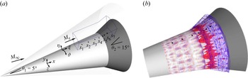
 p′
p′ uξ=0
uξ=0
 x=29.86cm
 {0,∞,e}
 x
x s8
s8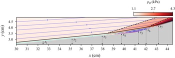
 qB
qB δ99
δ99 uξ,B=0
 s1
s1 s7
s7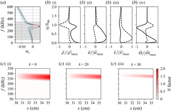
 αr
αr q˘
q˘ f,k
f,k qB
qB k=0
k=0 k=20
k=20 k=30
k=30 k=40
k=40 q˘n,m
q˘n,m N
N qB
qB
 in
in out
out w
w x
x η0
η0 f
f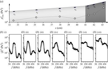
 prms2
prms2
 a
a γ
γ γ
γ b
b γ
γ (a)
(a) N
N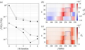
 J(c~0)
 J
J JS
JS JI
JI JP
JP b
b c
c N
N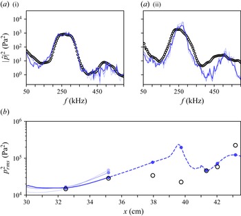
 s1
s1 s2
s2 x
x c~4
c~4 s3
s3 s7
s7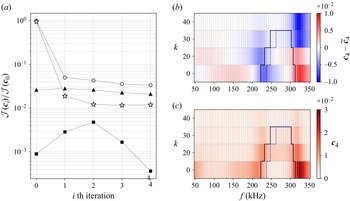
 J(c0)
J(c0) J
J JS
JS JI
JI JP
JP c0=c~4
 b
b c
c N
N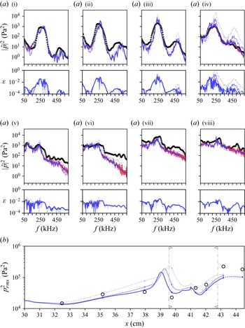
 s1
s1 s8
s8 ε
ε s8
s8 ε(f)
ε(f) ∑f|p^|2
 σi
σi 5%
5% c4
c4 x
x c0=c~4
 s7
s7 s8
s8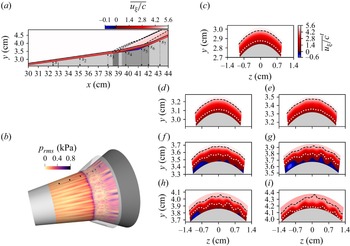
 q=N(c4)
 δ¯99
δ¯99 Υ(x,y)={1,0.5}
 x=[38.5,39.0]cm
 x=[39.4,42.1]cm
 Γ(x,ϑ)=0.5
 Υ(x,y)=1
 s1
s1 s7
s7
 xs¯
xs¯ xr¯
xr¯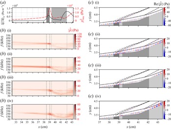
 q=N(c4)
 x=[38.5,39.0]cm
 x=[39.4,42.1]cm
 (f,k)
(f,k) f=250kHz
 δ¯99
δ¯99 Υ(x,y)=1
 Υ(x,y)=0.5
 uξ=0
uξ=0 k={0,20,30,40}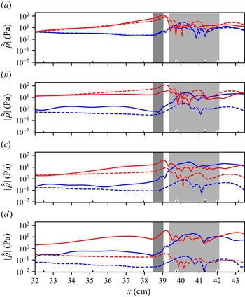
 (f,k)
(f,k) c4
c4 q=N(c4)
 qL′=Lq¯(c4)
 f=250kHz
 f=150kHz
 k={0,20,30,40}
 x=[38.5,39.0]cm
 x=[39.4,42.1]cm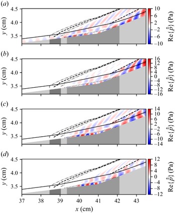
 f=150kHz
 a
a d
d k={0,20,30,40}
 x=[38.5,39.0]cm
 x=[39.4,42.1]cm
 δ¯99
δ¯99 Υ(x,y)=1
 Υ(x,y)=0.5
 uξ=0
uξ=0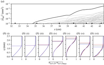
 q=N(c4)
 δ^99
δ^99 f={1,2,…,600}kHz
 f=5kHz
 b.i
b.i b.vii
b.vii u¯ξ
u¯ξ s1
s1 s7
s7 δ99
δ99 5T=1ms
 T=1/(5kHz)=0.2ms
 [t0,t0+T/2)
 [t0+T/2,t0+T)
 t0
t0 ⟨δ99⟩5kHz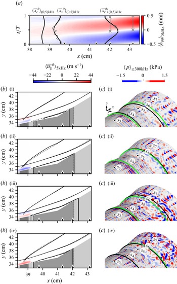
 q=N(c4)
 5kHz
5kHz ⟨δ99⟩5kHz
 ∙¯ϑ
∙¯ϑ 5kHz
5kHz ⟨∙¯ϑ⟩{0,5}kHz
 xc
xc xs
xs xr
xr [t0,t0+T/2)
 u¯ξ,1
u¯ξ,1 b
b 5kHz
5kHz δ99
δ99 t/T={0,0.25,0.5,0.75}
 5kHz
5kHz t=0
t=0 s4
s4 s7
s7 x=[38.5,39.0]cm
 x=[39.4,42.1]cm
 f≥300kHz
 x¯s
x¯s x¯r
x¯r ⟨x¯sϑ⟩{0,5}kHz
 ⟨x¯rϑ⟩{0,5}kHz
 s3
s3 s7
s7 t/T={0,0.25,0.5,0.75}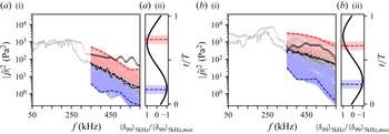
 a
a s6
s6 b
b s7
s7 q=N(c4)
 350
350 T/10=1/(50kHz)
 1/(1.75MHz)
 ∑350kHz600kHz|p^|2
 ⟨δ99⟩5kHz
 t0+T/20
 T/10
T/10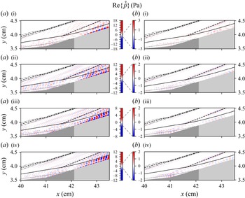
 f=450kHz
 k={0,20,30,40}
 T/10
T/10 [t0,t0+T/10)
 t0
t0 a
a s7
s7 (b.ii)
 t0
t0 b
b s7
s7 (b.ii)
 δ¯99
δ¯99 Υ(x,y)=1
 Υ(x,y)=0.5
 uξ=0
uξ=0 x=[39.4,42.1]cm
 Open access

