2. Mathematical formulation

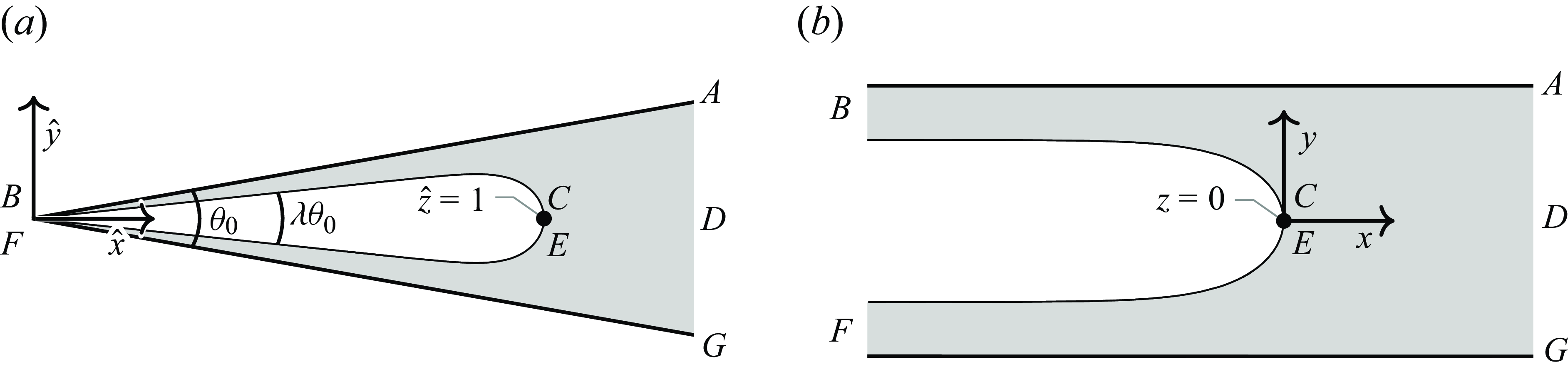
Consider a Hele-Shaw cell with very small thickness compared to the length. The cell has a wedge shape with internal angle $\theta _0$ , and is filled with viscous fluid. An inviscid fluid is injected from the corner of the wedge at a prescribed flow rate, and displaces the viscous fluid to form a petal/finger shape (figure 1 a). Eventually, as is seen experimentally (Thomé et al. Reference Thomé, Rabaud, Hakim and Couder1989), a self-similar shape is reached where a finger occupies an angle $\lambda \theta _0$ , with $0\lt \lambda \lt 1$ . Ben Amar (Reference Ben Amar1991a ) refers to this set-up as ‘divergent flow’.

On the free surface, we solve for $q\,\mathrm{e}^{-{i}\tau }$ (these are analogues of the speed $q$ and streamline angle $\tau$ , and reduce to the actual fluid speed and streamline angle in the limit $\theta _0 \rightarrow 0$ ) and finger shape $\hat {z} = \hat {x}+\mathrm{i} \hat {y}$ . We transform the self-similar physical plane $\hat {x} + \mathrm{i} \hat {y}$ (figure 1) into an infinite strip in a channel using the conformal map

(2.1) \begin{equation} z = \tfrac {2}{\theta _0} \log (\hat {z}). \end{equation}

In figure 1(b), we show the image of the finger from figure 1(a) under this map. The walls $BA$ and $FG$ lie on $\mathrm{Im}(z)= \pm 1$ , respectively, and the tip $CE$ is fixed at the origin $z=0.$

Figure 1. (a) Top-down view of the numerically obtained physical profile in the $\hat {z}$ -plane for the zero surface tension case with $\theta _0 = 20^{\circ }$ and $\lambda = 0.6$ . The Hele-Shaw cell is bounded by the thick black lines and is filled with a viscous fluid (grey). An inviscid fluid is injected from the corner of the wedge ( $BF$ at $\hat {z}=0$ ) and forms a finger with angle $\lambda \theta _0$ . The tip of the finger lies at $\hat {z}=1$ ( $CE$ ). (b) A numerical plot of the $z$ -plane (obtained using the mapping (2.1)) is shown for the zero surface tension case with $\theta _0 = 20^\circ$ and $\lambda = 0.6.$ The tip of the finger lies at the origin ( $CE$ ).

The independent variable is given as in Vanden-Broeck (Reference Vanden-Broeck1983), by $s = \mathrm{e}^{-\unicode{x03C0} f^*}.$ Here, $f^*$ is a generalised velocity potential as defined in Ben Amar (Reference Ben Amar1991a , p. 43), and is chosen so that the streamline value $\mathrm{Im}(f^*)$ is constant on the free surface. Under this map, half the free surface ( $BC$ ) lies on the real $s$ -axis between 0 and 1, with the finger tip ( $C$ ) at $s = 1$ .

We require a set of governing equations for the unknowns $(x(s), y(s), q(s), \tau (s))$ . Once these are solved for numerically, we can obtain a profile for the free surface in the physical wedge, $\hat {x}+\mathrm{i}\hat {y}$ , by reversing (2.1).

First, on the free surface, continuity of pressure yields Bernoulli’s equation

(2.2) \begin{equation} \epsilon ^2 \frac {\lambda }{Q_0}qs\, \frac {\partial }{\partial s} \left (r(x) \left [qs\frac {\partial \tau }{\partial s} + \frac {\ell }{2} \sin \tau \right ]\right ) - q = \frac {q}{1-\lambda } + \frac {q\lambda }{\unicode{x03C0} Q_0}\int _0^1\!\!\!\!\!\!\!\!-\ \,\frac {K(t)}{t-s}\,\mathrm{d}{t}. \end{equation}

In (2.2), we have defined the following functions for convenience:

(2.3) \begin{equation} r(x(s)) = \exp({-\theta _0\, x(s)/2}) \quad \text{and} \quad K(s) = \frac {\sin [\tau (s)] }{q(s)\, [r(x(s))]^2}. \end{equation}

In (2.2), we have also defined the dimensionless fluid flux constant $Q_0$ , and the scaled interior wedge angle $\ell$ , to be

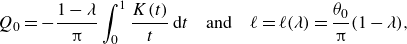(2.4) \begin{equation} Q_0 = -\frac {1-\lambda }{\unicode{x03C0} } \int _0^1 \frac {K(t)}{t} \, \mathrm{d}{t} \quad \text{and} \quad \ell = \ell (\lambda ) = \frac {\theta _0}{\unicode{x03C0} }(1-\lambda ), \end{equation}

where $\lambda$ is the proportional finger angle parameter. Finally, we have introduced the key non-dimensional parameter $\epsilon$ by

(2.5) \begin{equation} \epsilon ^2 = \frac {4\unicode{x03C0} ^2 \sigma }{(1-\lambda )^2}, \end{equation}

where $\sigma$ is a modified surface tension parameter

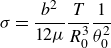(2.6) \begin{equation} \sigma = \frac {b^2}{12\mu } \frac {T}{R_0^3}\frac {1}{\theta _0^2} \end{equation}

as in Ben Amar (Reference Ben Amar1991b ). Here, $b$ is the distance between the plates in the Hele-Shaw cell, $\mu$ is viscosity, $T$ is surface tension, and $R_0$ is a length scale parameter (the length from the wedge corner to the tip of the finger at time zero). Typically, we are interested in small surface tension, thus small values of $\epsilon$ .

Analyticity of $q\,\mathrm{e}^{-\mathrm{i} \tau }$ in the upper half $s$ -plane gives, by the Hilbert transform,

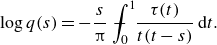(2.7) \begin{equation} \log q(s) = -\frac {s}{\unicode{x03C0} }\int _0^1\!\!\!\!\!\!\!\!-\ \,\frac {\tau (t)}{t(t-s)}\,\mathrm{d}{t}. \end{equation}

Finally, we close the system with

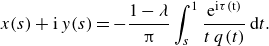(2.8) \begin{equation} x(s) +\mathrm{i}\, y(s) = -\frac {1-\lambda }{\unicode{x03C0} }\int _s^1 \frac {\mathrm{e}^{\rm{i}\tau (t)}}{t\,q(t) } \, \mathrm{d}{t}. \end{equation}

Thus the full system consists of equations (2.2), (2.7) and (2.8) for the unknowns $(x, y, q, \tau )$ . The appropriate boundary conditions at $s=0$ and $s=1$ are

(2.9a) \begin{align} x(0) = - \infty , \quad y(0) = 1, \quad q(0) = 1, \quad \tau (0) & = 0, \end{align}

(2.9b) \begin{align} x(1) = 0, \quad y(1) = 0, \quad q(1) = 0, \quad \tau (1) & = -\frac {\unicode{x03C0} }{2}. \end{align}

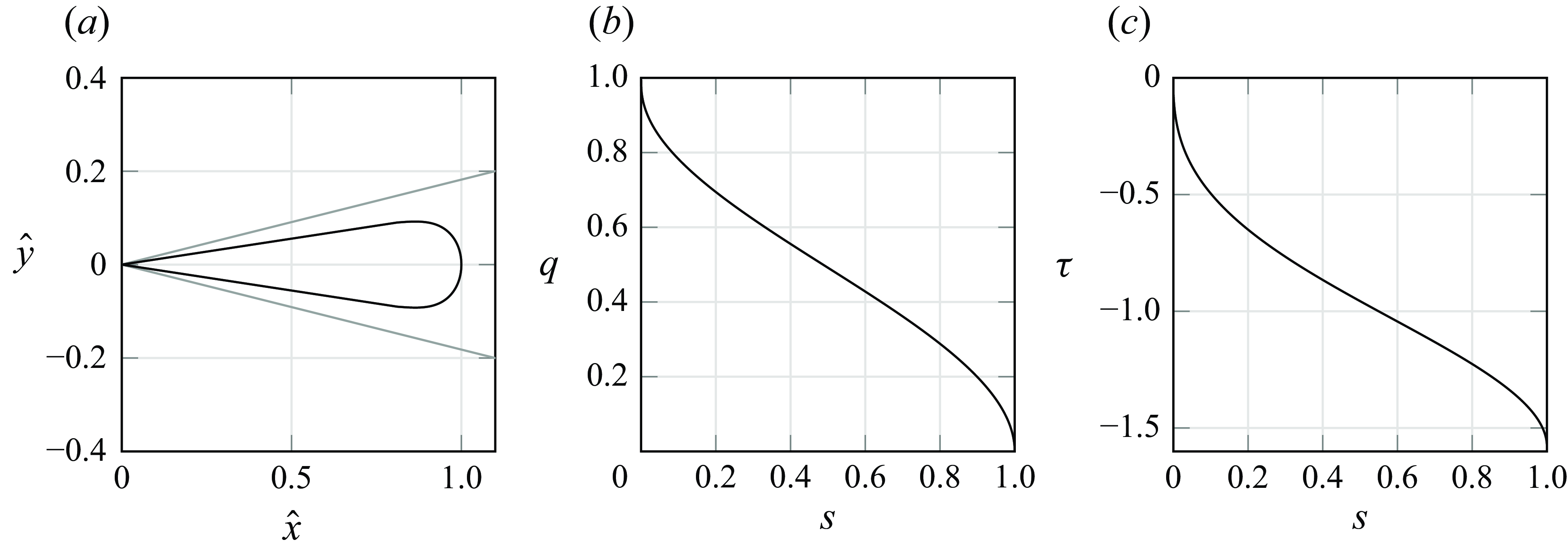
The governing equations can be compared with Ben Amar (Reference Ben Amar1991b ) equations (3.15)–(3.17). An example of the numerically obtained solutions for $\theta _0 =20^\circ$ , $\epsilon ^2 =1$ and $\lambda =0.64$ is shown in figure 2.

Figure 2. (a) Plot of a numerical solution shown in the $(\hat {x}, \hat {y})$ -plane in the wedge. (b,c) Plots of the numerical solutions for the dependent variables $q(s),\tau (s)$ . In this figure, the parameter values are $\theta _0 = 20^\circ$ , $\epsilon ^2 = 1$ and $\lambda =0.64$ .

We note that following Ben Amar (Reference Ben Amar1991a ), the mathematical model of divergent flow developed here produces a steady-state formulation corresponding to an assumption of self-similarity of the original system. In particular, the spatial coordinates of the original system are assumed to scale with a time-dependent dimensionless scaling factor ((2.1) of Andersen et al. Reference Andersen, Lustri, McCue and Trinh2024).

3. Exponential asymptotics

We briefly present the exponential asymptotics method that can be used to derive the selection condition in the limit $\epsilon \rightarrow 0$ . The full details of this are presented in Andersen et al. (Reference Andersen, Lustri, McCue and Trinh2024), but we compare their results to our numerical results in § 6. The exponential asymptotic analysis involves approximating the dependent variables as asymptotic series in the small parameter $\epsilon$ ,

(3.1) \begin{align} x \sim \sum _{n=0}^\infty \epsilon ^{2n}x_n, \quad y \sim \sum _{n=0}^\infty \epsilon ^{2n}y_n, \quad q \sim \sum _{n=0}^\infty \epsilon ^{2n}q_n, \quad \tau \sim \sum _{n=0}^\infty \epsilon ^{2n}\tau _n. \\[9pt] \nonumber \end{align}

The leading-order solutions $\{x_0, y_0, q_0, \tau _0\}$ are found analytically as shown in Andersen et al. (Reference Andersen, Lustri, McCue and Trinh2024) equations (3.7) and (3.8). A plot of the leading-order physical profile $(x_0,y_0)$ is shown later, in figure 5. The asymptotic series in (3.1) turn out to be divergent, and it is necessary to truncate them. If this is done at an optimal point $n=\mathcal{N}$ , then the remainder will be a sum of contributions that are exponentially small in the surface tension parameter $\epsilon$ . For example, $q$ will have the form

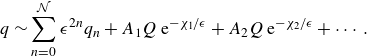(3.2) \begin{equation} q \sim \sum _{n=0}^{\mathcal{N}} \epsilon ^{2n}q_n + A_1 Q\, \mathrm{e}^{-\chi _1/\epsilon } + A_2 Q\, \mathrm{e}^{-\chi _2/\epsilon } + \cdots . \end{equation}

Exponential asymptotics techniques can be used to derive the forms of the components $A_i,$ $Q$ and $\chi _i$ as functions of $s$ . These are given in terms of a different independent variable, $\zeta$ , in Andersen et al. (Reference Andersen, Lustri, McCue and Trinh2024) (equations (6.16), (5.9) and (5.7)), where

(3.3) \begin{equation} s = \frac {1}{\zeta ^2+1}. \end{equation}

The functions $\chi _i$ are complex functions and are given in terms of $\zeta$ by

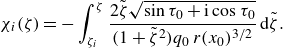(3.4) \begin{equation} \chi _i(\zeta ) = -\int _{\zeta _i}^\zeta \frac {2\tilde {\zeta }\sqrt {\sin \tau _0 + \mathrm{i} \cos \tau _0}}{(1+\tilde {\zeta }^2) q_0\, r(x_0)^{3/2}}\,{\rm d}\tilde {\zeta }. \end{equation}

Here, $\zeta _i$ are locations of singularities in the complex $\zeta$ -plane (e.g. for $\theta _0 = 20^\circ$ , $\lambda =0.75$ , there is a singularity at $\zeta _1=0.62+3.01\mathrm{i}$ ). Since the $\chi _i$ are complex, the remainder terms introduce exponentially small oscillations in the solution with amplitudes $|A_i Q|\,\mathrm{e}^{-\mathrm{Re}(\chi _i)/\epsilon }$ . These oscillations can be seen on the tips of the fingers in figure 5. By enforcing the far-field boundary conditions (2.9a ) on the remainder terms, it is possible to obtain the selection condition

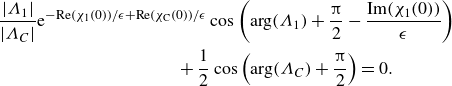(3.5) \begin{align} & \frac {|\Lambda _1|}{|\Lambda _{{C}}|} \rm {e}^{-\mathrm{Re}(\chi _1(0))/\epsilon +\mathrm{Re}(\chi _{{C}}(0))/\epsilon } \cos \left (\arg (\Lambda _1) + \frac {\unicode{x03C0} }{2} - \frac {\mathrm{Im}(\chi _1(0))}{\epsilon }\right )\nonumber\\ &\qquad\qquad\qquad\qquad\qquad + \frac {1}{2}\cos \left (\arg (\Lambda _{{C}}) + \frac {\unicode{x03C0} }{2}\right ) = 0. \end{align}

By symmetry arguments, only remainder terms related to two singularities (indexed ‘ $1$ ’ and ‘ $C$ ’) contribute to the selection condition. The constants $\Lambda _1$ and $\Lambda _{{C}}$ can be found with further analysis (see Appendix C of Andersen et al. Reference Andersen, Lustri, McCue and Trinh2024). Bifurcation diagrams can be plotted showing the solutions that satisfy (3.5), and these are presented in figure 8 in § 6 as a comparison to our numerical results.

4. Channel problem ( $\boldsymbol{\theta} _{\boldsymbol{0}} = \boldsymbol{0}$ )

By taking the limit of the wedge angle, $\theta _0 \rightarrow 0$ , we recover the classic Saffman–Taylor problem in a channel with parallel walls. This exhibits a similar selection mechanism for the relative finger widths, $0.5\lt \lambda _1\lt \lambda _2\lt \lambda _3\lt \cdots \lt 1$ . The problem was solved numerically by McLean & Saffman (Reference McLean and Saffman1981) and Vanden-Broeck (Reference Vanden-Broeck1983), who plotted bifurcation diagrams of the selected $\lambda$ values against the surface tension parameter $\epsilon ^2$ . We have replicated their numerical method to generate the bifurcation diagram in figure 3.

The analysis in § 3 can also be repeated for the simpler problem in a channel that is equivalent to taking the limit $\theta _0 \rightarrow 0$ in (3.5). The selection condition for the channel was first derived using exponential asymptotic techniques in Chapman (Reference Chapman1999), and the selected $\lambda$ values are presented in figure 3.

This comparison of numerical and exponential asymptotic results for the channel problem is currently missing from the literature. We see that the results agree well except for very small values of $\epsilon$ where larger numbers of mesh points in the numerical scheme would reduce the numerical errors. The Saffman–Taylor problem in a wedge poses additional difficulties in both the numerics and asymptotic analysis since the Bernoulli equation becomes more complex. In § 5, we describe a numerical method that can obtain numerical solutions of the wedge problem, and in § 6, we compare the bifurcation diagrams with recent exponential asymptotic results.

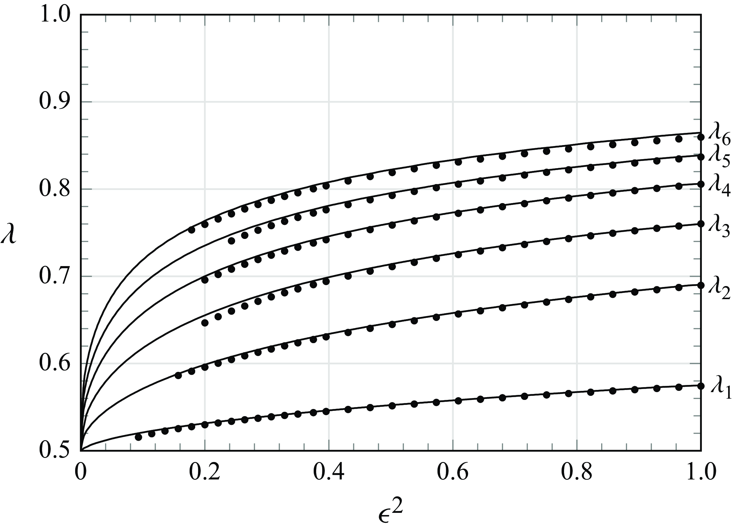
Figure 3. Bifurcation diagram for the Saffman–Taylor problem in a channel ( $\theta _0 = 0$ ) showing the first six selected $\lambda$ values for different values of the surface tension parameter $\epsilon ^2$ . The black curves show the predicted branches from the exponential asymptotic analysis as done in Chapman (Reference Chapman1999). The dots show the branches predicted using an implementation of the numerical scheme from McLean & Saffman (Reference McLean and Saffman1981) and Vanden-Broeck (Reference Vanden-Broeck1983) with $N=1000$ mesh points.

5. Numerical methodology

Our numerical method is a generalisation of methods from McLean & Saffman (Reference McLean and Saffman1981) and Vanden-Broeck (Reference Vanden-Broeck1983), but with additional difficulties from the increased complexity of the equations. First, we relax the condition for the angle at the tip of the finger, $\tau (1)$ , in (2.9b ) so $\tau (1)$ becomes a free parameter to be solved for as part of the solution. We then solve for the physical profile at all combinations of $\epsilon ^2$ and $\lambda$ . Each of these solutions will have an associated $\tau (1)$ value. Selecting the solutions with $\tau (1)=-\unicode{x03C0} /2$ will give the physical fingers with a smooth tip. We now describe the scheme in more detail.

Following McLean & Saffman (Reference McLean and Saffman1981) and Vanden-Broeck (Reference Vanden-Broeck1983), we introduce a stretched mesh from $s \mapsto \xi$ defined by

(5.1) \begin{equation} s^\rho = 1-\xi ^\gamma , \end{equation}

where $\rho$ solves the equation

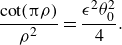(5.2) \begin{equation} \frac {\cot (\unicode{x03C0} \rho )}{\rho ^2} = \frac {\epsilon ^2 \theta _0^2}{4}. \end{equation}

The parameter $\gamma$ defines the distribution of mesh points, with a larger $\gamma$ meaning that more points are distributed near the tip of the finger. For the results in this paper, we choose $\gamma =4,$ as is done in Vanden-Broeck (Reference Vanden-Broeck1983). A larger value of $\gamma$ means that more accurate results can be achieved with fewer mesh points. If $\gamma$ becomes too large (e.g. $\gamma \gtrsim 5$ ), then the numerical scheme fails to converge.

The principal mesh points and their related midpoints are respectively defined by $\xi _j = j/N$ for $j=0,1,\ldots ,N$ , and $\xi _j^m = (2j-1)/2N$ for $j=1,2,\ldots ,N$ , and the corresponding points in the $s$ -plane are found using (5.1). The unknowns are the values of $\tau$ at the mesh points, which we denote $\tau _j = \tau (s_j)$ with $j=0,1,\ldots ,N.$ The condition $\tau (0) = 0$ from (2.9 a ) fixes $\tau _N = 0$ . We allow $\tau _0= \tau (1)$ to be a free parameter, so we have $N$ unknowns, $\tau _0,\ldots , \tau _{N-1}$ . We will similarly use subscripts when evaluating other variables at mesh points, i.e. $q_j = q(s_j)$ , $x_j= x(s_j)$ and $y_j = y(s_j)$ .

The main step in the numerical scheme is evaluating (2.2) at the $N-1$ internal mesh points, $s_1,\ldots , s_{N-1}$ , to give $N-1$ equations:

(5.3) \begin{equation} \epsilon ^2 s_j \left (r(x_j)\left [q_j s_j \tau^{\prime}_j + \frac {\ell }{2}\sin \tau _j\right ]\right )^{\prime}+\frac {Q_0}{1-\lambda } + \frac {1}{\unicode{x03C0} }I(s) = 0, \quad j = 1,\ldots, N-1. \end{equation}

In (5.3), we have used the definitions of $r(x)$ from (2.3) and $\ell$ from (2.4). It is also convenient to define the integral

(5.4) \begin{equation} I(s) = {\int}_{\kern-5pt 0}^{\kern-1pt 1} \kern-15.5pt - \ \frac {K_j(t)}{t-s}\,\mathrm{d}{t}, \end{equation}

where $K_j = K(s_j)$ . We use trapezoidal rules to evaluate the integrals in (5.3) from $x_j$ (2.8), $q_j$ (2.7), $Q_0$ (2.4) and $I$ .

We have defined $N-1$ equations in (5.3) for the $N$ unknowns $(\tau _0, \ldots , \tau _{N-1}).$ To close the system, we introduce one final equation, which is given by evaluating the trapezoidal approximation of (2.8) in the far-field, at $s=0$ ,

(5.5) \begin{equation} \lambda - \mathrm{Im} \left [\frac {1-\lambda }{\unicode{x03C0} N} \sum _{k=1}^{N-1} \frac { \sin (\tau _k)\,s^{\prime}_k}{s_k q_k}\right ]=0. \end{equation}

That is, (5.3) and (5.5) give $N$ equations that can be solved for the $N$ unknowns using a Newton iteration scheme.

In practice, the evaluation of the equations is computationally intense due to the number of integrals approximated with trapezoidal rules. The Jacobian matrix is dense, so the equations must be evaluated many times at each step.

In order to speed up the scheme, we use Broyden’s method (Broyden Reference Broyden1965), which is a quasi-Newton method. Broyden’s method evaluates the Jacobian only on the first step, then updates the associated matrix to approximate the Jacobian at later steps. However, the method requires a much closer initial guess than Newton’s method to converge. We therefore implement a scheme that uses Newton’s method at low $N$ values (typically $N = 250$ ) to provide an interpolated approximation for the initial guess to the Broyden scheme at higher values of $N$ (e.g. $N = 500$ ). We continue doubling $N$ , interpolating the solution and solving with Broyden until we reach the desired value of $N$ . 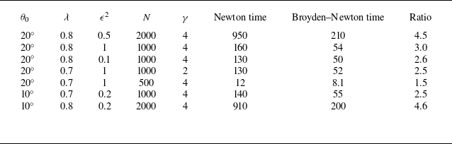Using this scheme, we can obtain a solution for $N=2000$ almost five times faster than using pure Newton’s method. The run times of this scheme compared to the standard Newton’s method are shown in table 1. We find that the convergence rate of the numerical scheme is $\mathcal{O}(1/N)$ as $N \rightarrow \infty$ , therefore a large value of $N$ is needed to obtain accurate results.

Table 1. Times in seconds (given to two significant figures) for the pure Newton method compared to our adapted Broyden–Newton method.

6. Numerical results

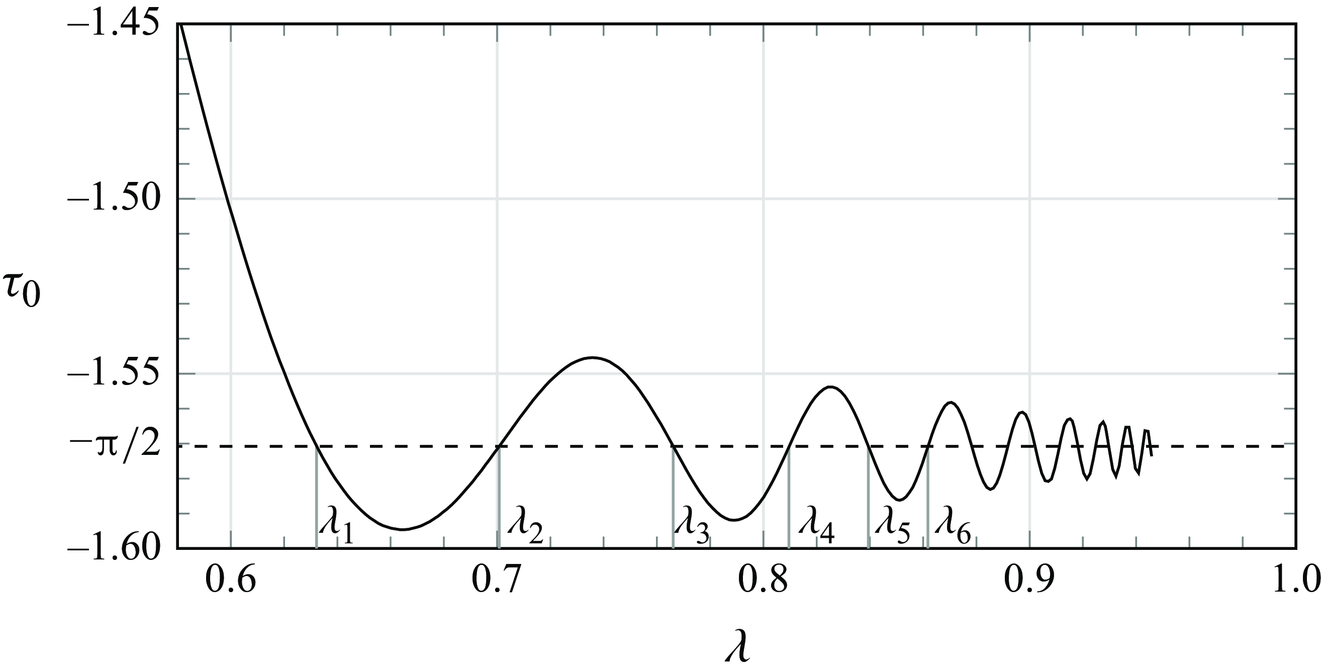
The numerical method allows the angle at the tip of the finger ( $\tau _0$ ) to be a free parameter. However, the solutions are physical only if they are smooth, which requires the tip of the finger to have angle $-\unicode{x03C0} /2$ . In figure 4, we plot the angle at the tip of the finger against $\lambda$ for $\epsilon ^2=1$ , $\theta _0 = 20^\circ$ . We can identify the selected $\lambda$ values, $\lambda = \lambda _1, \lambda _2, \ldots $ , at which $\tau _0 = -\unicode{x03C0} /2$ .

Figure 4. Plot of the angle at the tip of the finger versus $\lambda$ for $\epsilon ^2 = 1,$ $\theta _0 = 20^\circ$ . Smooth, physical fingers exist at the intersection points where $\tau _0=-\unicode{x03C0} /2$ . The asymptotic analysis of the selection mechanism (Andersen et al. Reference Andersen, Lustri, McCue and Trinh2024) shows that there exists a countably infinite number of such selected fingers with associated $\lambda$ values labelled $\lambda _1(\epsilon )\lt \lambda _2(\epsilon )\lt \lambda _3(\epsilon )\lt \cdots \lt 1$ .

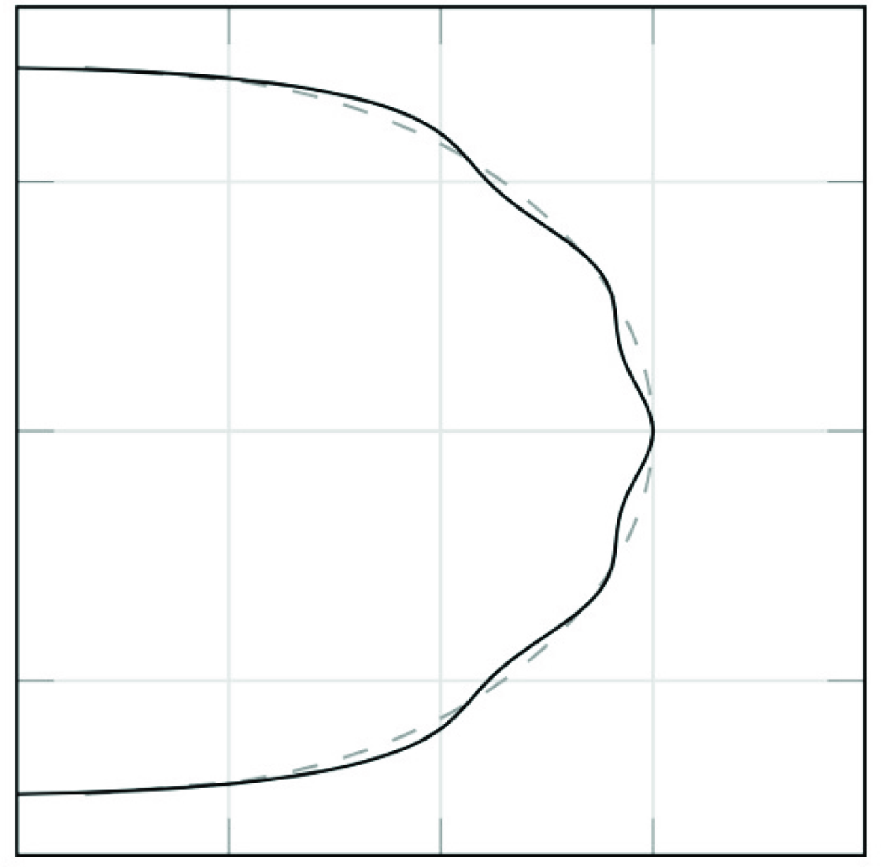
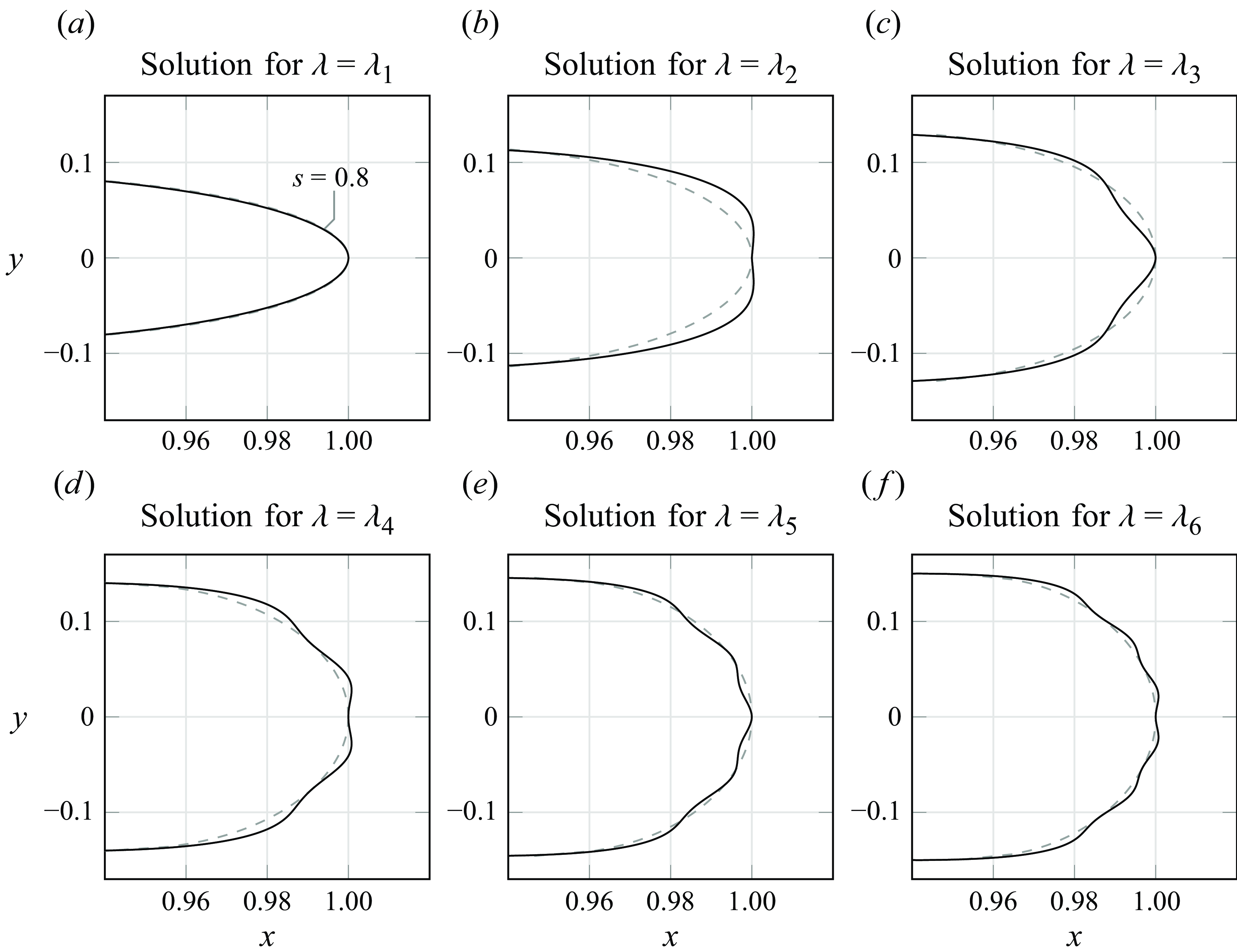
The physical profiles for the first six selected solutions are shown in figure 5 for $\epsilon ^2 = 3$ , $\theta _0 = 20^\circ$ . The figure shows that small oscillations appear in the profiles near the tips of the fingers. We also see that each successive selected value of $\lambda (\epsilon )$ has an associated physical profile with one additional wavelength of oscillations at the tip. The selection condition can be obtained analytically by analysing these exponentially small contributions to the solution using the techniques from exponential asymptotics. This analysis is done in a separate paper (Andersen et al. Reference Andersen, Lustri, McCue and Trinh2024), and the key ideas were briefly summarised in § 3.

Figure 5. Numerical solutions showing the physical profiles (black) for the first six selected solutions with $\epsilon ^2=3$ , $\theta _0 = 20^\circ$ . The interface develops oscillations near the tip of the finger for the higher branches. Here, $\epsilon = 3$ is chosen since this is large enough for the oscillations to be visible. The leading-order solution $(x_0,y_0)$ is shown in grey.

Figure 6. Plot of $\tau -\tau _{{leading}}$ showing the exponentially small oscillations in the solution. The amplitudes of the oscillations are approximated at $s=0.8$ by interpolating from neighbouring peaks, and the approximated amplitudes are plotted in figure 7 for different values of $\epsilon$ .

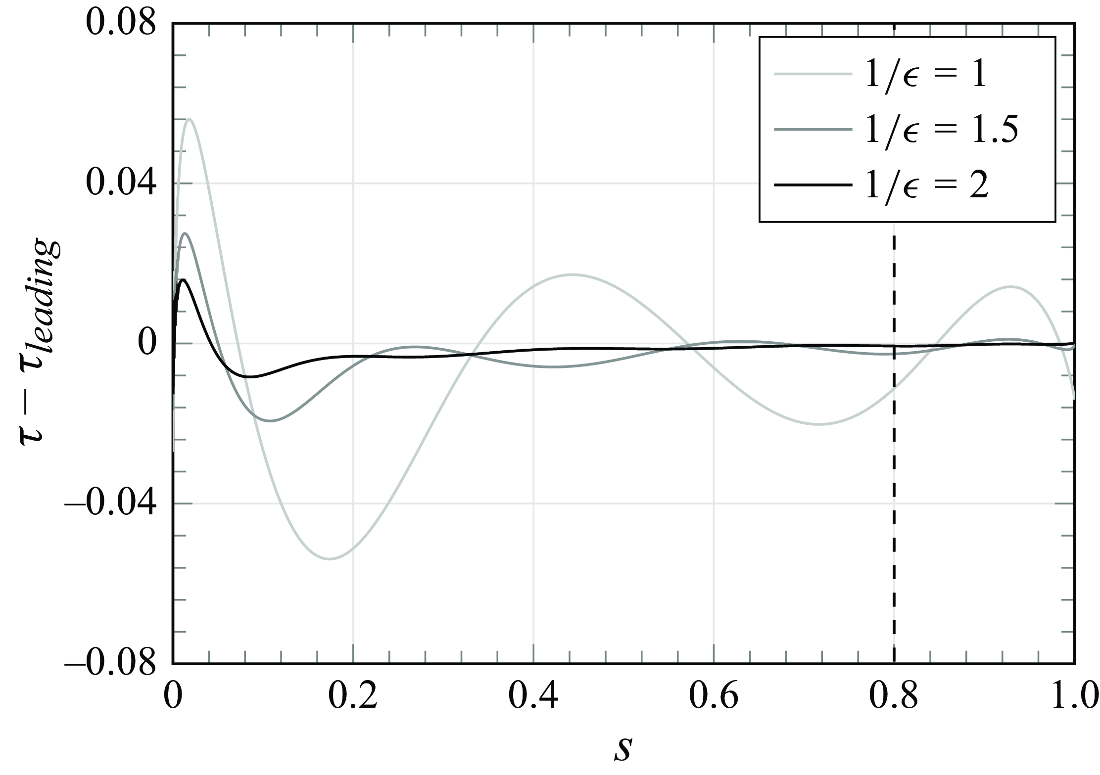
We can measure the amplitude of the oscillations near the tip as $\epsilon$ varies. For each value of $\epsilon$ , we fix $\lambda =0.85$ and then use our numerical method to find $\tau$ along the free surface. We subtract the leading-order component of $\tau$ , associated with zero surface tension, which makes the oscillations easier to identify, as shown in figure 6. The amplitude of the oscillations varies with $s$ , so we measure the amplitudes at a fixed value $s=0.8$ , which lies near the tip of the finger. Since $s=0.8$ does not necessarily fall at a peak of the oscillations, this requires an approximation of the amplitude, which we obtain by interpolating from the amplitudes of the neighbouring peaks. The approximated oscillation amplitude versus $1/\epsilon$ is shown in figure 7.

Figure 7. The amplitude of the small oscillations shown in figure 5, measured via $\tau$ at $s=0.8$ as a function of $\epsilon$ . These correspond to computations with $N=1000$ , $\lambda =0.85$ and $\theta _0 = 5^\circ , 20^\circ$ . The straight line shows the line of best fit (approximate gradient −4.6 for $\theta _0=20^\circ$ , and −4.3 for $\theta _0=5^\circ$ ), confirming exponential smallness in $\epsilon$ . The predicted gradient (−5.9 for $\theta _0=20^\circ$ , and −4.8 for $\theta _0 = 5^\circ$ ) from the exponential asymptotics for $\theta _0=20^\circ$ is also shown.

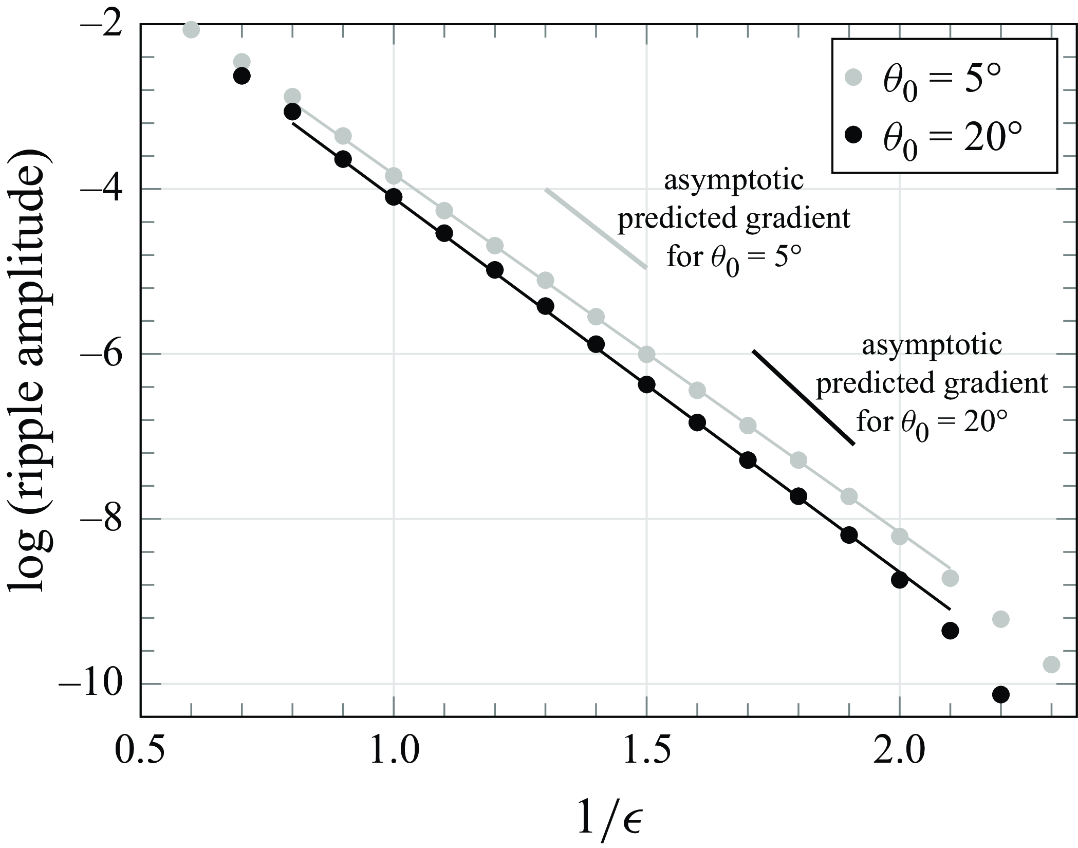
We see in figure 7 that for a range $1/\epsilon \approx 0.9{-}1.9$ , the logarithm of the oscillation amplitudes follows a straight line with negative gradient (approximate gradient −4.6 for $\theta _0=20^\circ$ , and −4.3 for $\theta _0=5^\circ$ ). This shows that the measured oscillations are exponentially small with respect to the surface tension parameter $\epsilon$ , in the limit $\epsilon \rightarrow 0$ . For $\theta _0=20^\circ$ , the predicted gradient from the exponential asymptotics is −5.9, and for $\theta _0=5^\circ$ , the predicted gradient is −4.8.

For larger $\epsilon$ values, it is expected that figure 7 will cease to be linear, as the small $\epsilon$ approximation breaks down, and nonlinear components will begin to dominate. For smaller $\epsilon$ values, the oscillations on the profile become very small and are difficult to identify. To measure the amplitude of these oscillations, we would first need to subtract out the $\mathcal{O}(\epsilon )$ trends; however, the complexity of numerical solutions of higher-order algebraic corrections rivals that of the full nonlinear problem.

Finally, we use the numerical method to find the selected solutions with a smooth tip ( $\tau _0 = -\unicode{x03C0} /2$ ), and use numerical continuation to follow the families of selected solutions $\lambda _i(\epsilon )$ for decreasing values of $\epsilon$ . Values for these selected families of $\lambda _i(\epsilon ),$ $ i =1,2,\ldots$ , are plotted in bifurcation diagrams in figure 8 using $N=1000$ mesh points. The bifurcation diagrams are compared to exponential asymptotic results from Andersen et al. (Reference Andersen, Lustri, McCue and Trinh2024) in figures 8(a)–8(c) for three different wedge angles. We see good agreement between the numerical results and the exponential asymptotics, particularly for higher branches and larger values of $\epsilon ^2$ .

Figure 8. Bifurcation diagrams for wedge angles (a) $\theta _0 = 5^\circ$ , (b) $\theta _0 = 10^\circ$ and (c) $\theta _0 = 20^\circ$ , showing the first six selected $\lambda$ values for different values of the surface tension parameter $\epsilon ^2.$ The black curves show the predicted branches found by evaluating (3.5) from the exponential asymptotic analysis in Andersen et al. (Reference Andersen, Lustri, McCue and Trinh2024). The dots show the branches predicted using the numerical scheme described in § 5 with $N=1000$ mesh points. The numerical scheme is able to solve for higher branches than the results of previous numerics for this problem presented in Ben Amar (Reference Ben Amar1991b ) for $\theta _0 = 20^\circ$ . (d) Zoom in on the third and fourth branches from the bifurcation diagram for $\theta _0 = 20^\circ$ with numerical results (dots) for $N=500$ (light grey), $N=1000$ (grey), $N=2000$ (black) mesh points.

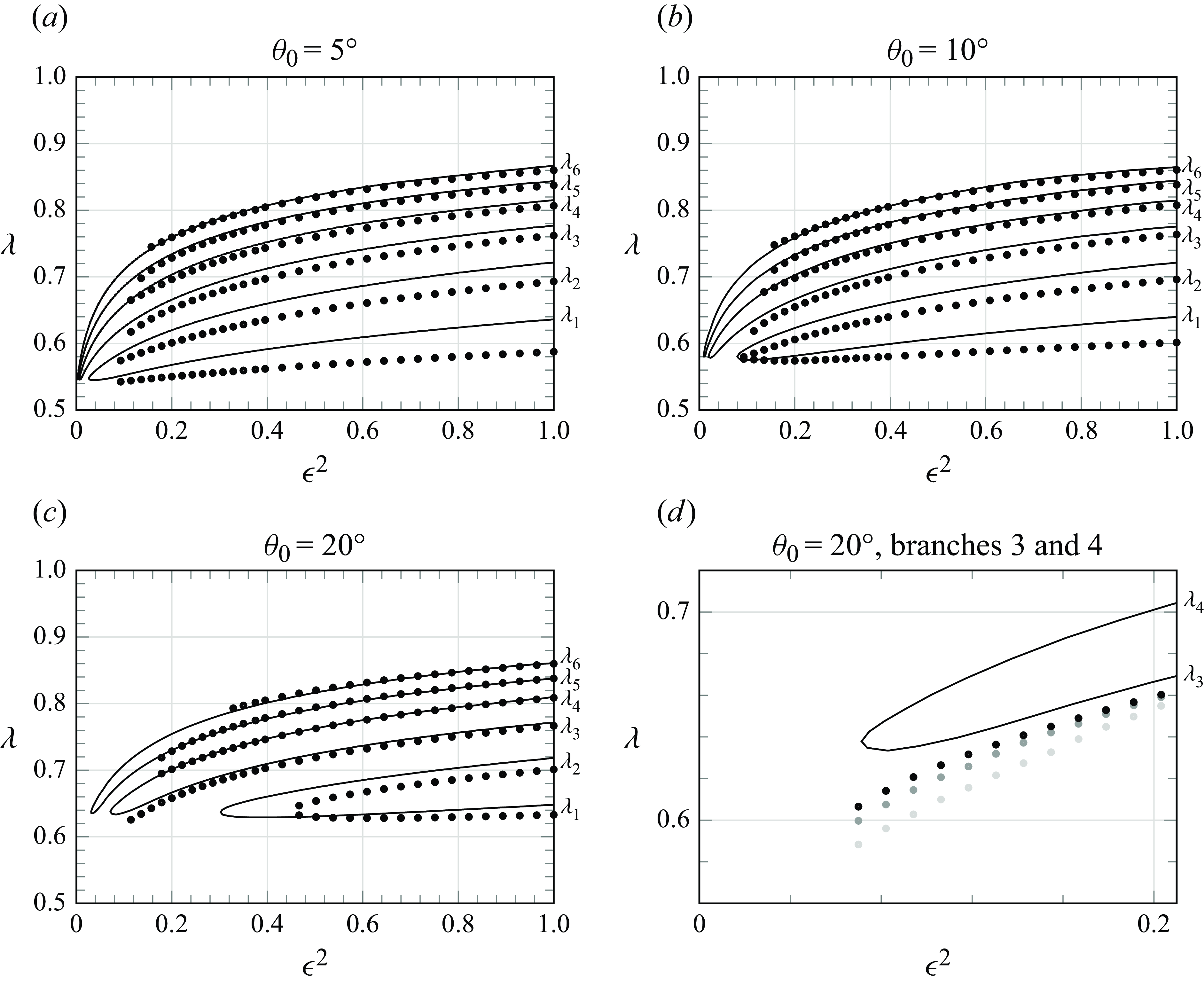
A numerical error occurs for small $\epsilon$ values; however, in figures 8(a)–8(c), we have omitted the numerical results when this error is large. The error is demonstrated in figure 8(d) for the third branch, $\lambda _3$ , in the case with $\theta _0=20^\circ$ . Here, the error between the numerical results and exponential asymptotic results increases significantly when $\epsilon ^2\lt 0.1$ . As shown in figure 8(d), with $N=500, 1000, 2000$ , the accuracy can be improved for small $\epsilon$ values by increasing the number of mesh points. We have found the error to be $\mathcal{O}(1/N)$ as $N\rightarrow \infty$ , so a very large number of mesh points would be needed to accurately resolve the bifurcation diagram at low values of $\epsilon ^2$ .

Further, figures 8(a)–8(c) show that the agreement between the exponential asymptotic results and the numerical results improves for the higher branches. We conjecture that one of the assumptions in the asymptotic theory is violated for the lower branches. The selection condition (3.5) is based on two singularities, $\zeta _1$ and $\zeta _{{C}}$ , in the complex $\zeta$ -plane. In addition, there are branch points at $\zeta = \pm \mathrm{i}$ . In the dual limit as $\lambda \rightarrow 0.5$ and $\theta _0 \rightarrow 0$ , the singularity $\zeta _1$ approaches the branch point at $\mathrm{i}$ . The exponential asymptotic analysis relies on the assumption that the singularities in the complex plane are well separated, and this breaks down in the dual limit. We conjecture that a special regime needs to be considered when the singularity $\zeta _1$ enters the neighbourhood of the branch point at $\zeta = \mathrm{i}$ , and that this would improve the exponential asymptotic results on the lower branches.