





1. Introduction
An important, if not universal, property of three-dimensional (3-D) boundary layers is that in these flows the direction of the mean velocity vector changes with distance from the wall (e.g. Littell & Eaton Reference Littell and Eaton1994). In general, the study of wall-bounded turbulent flows benefits many engineering and scientific applications, such as predicting drag force, optimising heat transfer in systems and controlling fluid flow in industrial processes. This includes boundary layers subjected to cross-flow effects, since in most applications the flow is not purely two-dimensional. Cross-flow also affects the turbulence structure in flow over swept-wing aircraft (see Saric et al. Reference Saric, Reed and White2003), and in the implementation of drag reduction strategies (see Quadrio Reference Quadrio2011). The rotating disk boundary layer (RDBL) serves as a suitable model for the fundamental study of the effects of three-dimensionality on the structure of a turbulent boundary layer (TBL). This is because RDBL has an exact similarity solution to the Navier–Stokes equations in the laminar regime, first introduced by von Kármán (Reference von Kármán1921), and this flow is inherently three-dimensional due to the intrinsic contribution of the cross-flow component in the spanwise (radial) direction. The RDBL has some distinctive features, making it an ideal subject for the study of turbulent wall flows. There is no pressure gradient in the streamwise/tangential direction. This flow, however, undergoes an acceleration in the radial direction due to the presence of the centrifugal force (CF). Therefore, it provides a ‘canonical’ context for studying 3-D wall flows.
The RDBL has been the subject of numerous stability analyses and laminar to turbulent transition studies (e.g. Appelquist et al. Reference Appelquist, Schlatter, Alfredsson and Lingwood2018a
). Relatively fewer works have, however, explored the rotating disk turbulent boundary layer (RDTBL), especially at high Reynolds numbers. Itoh & Hasegawa (Reference Itoh and Hasegawa1994) and Littell & Eaton (Reference Littell and Eaton1994) conducted hot-wire studies of air flow over a 1 m rotating disk up to $Re=r(\varOmega /\nu )^{1/2}=1265$
. This Reynolds number definition is typically used for laminar flow and stability investigations, where
$Re=r(\varOmega /\nu )^{1/2}=1265$
. This Reynolds number definition is typically used for laminar flow and stability investigations, where $r$
and
$r$
and $\varOmega$
represent the radial distance from the disk centre and the angular velocity of the disk, respectively, and
$\varOmega$
represent the radial distance from the disk centre and the angular velocity of the disk, respectively, and $\nu$
denotes the kinematic viscosity of the fluid. Their studies included the measurement of mean radial and tangential velocities and the six Reynolds stresses. Using the hot-wire anemometry technique, Imayama et al. (Reference Imayama, Alfredsson and Lingwood2012) found that a fully turbulent flow over an infinite rotating disk is attained at
$\nu$
denotes the kinematic viscosity of the fluid. Their studies included the measurement of mean radial and tangential velocities and the six Reynolds stresses. Using the hot-wire anemometry technique, Imayama et al. (Reference Imayama, Alfredsson and Lingwood2012) found that a fully turbulent flow over an infinite rotating disk is attained at $Re\gt 650$
. The investigation of 3-D turbulent flow over a rotating disk is not limited to experimental measurements. Appelquist et al. (Reference Appelquist, Schlatter, Alfredsson and Lingwood2018b
) conducted the first direct numerical simulation (DNS) study of the RDTBL at
$Re\gt 650$
. The investigation of 3-D turbulent flow over a rotating disk is not limited to experimental measurements. Appelquist et al. (Reference Appelquist, Schlatter, Alfredsson and Lingwood2018b
) conducted the first direct numerical simulation (DNS) study of the RDTBL at $Re=669$
. The DNS data were compared with the Imayama et al. (Reference Imayama, Lingwood and Alfredsson2014) data for turbulent disk flow and the numerical findings of Schlatter & Örlü (Reference Schlatter and Örlü2010) for the 2-D zero-pressure-gradient (ZPG) TBL. To the authors’ knowledge, however, there has been no study of the mean momentum balance (MMB) structure or the stress balance (i.e. once-integrated MMB) of the RDTBL. Mean momentum balance is essentially the Reynolds-averaged Navier–Stokes equation, and in the case of the RDTBL, we have MMB in the dominant tangential (
$Re=669$
. The DNS data were compared with the Imayama et al. (Reference Imayama, Lingwood and Alfredsson2014) data for turbulent disk flow and the numerical findings of Schlatter & Örlü (Reference Schlatter and Örlü2010) for the 2-D zero-pressure-gradient (ZPG) TBL. To the authors’ knowledge, however, there has been no study of the mean momentum balance (MMB) structure or the stress balance (i.e. once-integrated MMB) of the RDTBL. Mean momentum balance is essentially the Reynolds-averaged Navier–Stokes equation, and in the case of the RDTBL, we have MMB in the dominant tangential ( $\theta$
) direction as well as in the radial (
$\theta$
) direction as well as in the radial ( $r$
) direction.
$r$
) direction.
The layer structure of a turbulent flow can be characterised by examining the force distribution in the MMB equation (Wei et al. Reference Wei, Fife, Klewicki and McMurtry2005). As such, this approach has been extensively employed to investigate a variety of wall-bounded turbulent flows (e.g. Klewicki et al. Reference Klewicki, Fife, Wei and McMurtry2007; Wei Reference Wei2020; Chin & Philip Reference Chin and Philip2021). Mean momentum analysis can provide insight into the dynamics of turbulent flows and is a basis to examine the mechanisms of momentum transport and the interaction between mean flow and turbulent fluctuations. Determining the leading terms in the MMB equation together with an appropriate scaling that preserves it independent of the Reynolds number are central steps in unravelling the physics and scaling of turbulent wall flows (Fife et al. Reference Fife, Klewicki and Wei2009).
For the RDTBL, von Kármán (Reference von Kármán1921) derived two stress balance equations at the disk surface in the tangential and radial directions. The first integral equation is based on the balance between the radial flux of the angular momentum and the torque applied to the disk by the mean tangential wall shear stress ( $\tau _{w_\theta }$
)
$\tau _{w_\theta }$
)
 \begin{align} 2\pi \rho \frac {\text{d}}{\text{d}r} \left ( r^{2} \int _{0}^{\infty } U_r U_\theta \, \text{d}y \right ) = -2\pi r^{2} \tau _{w_\theta }, \end{align}
where $U_r$
and
$U_r$
and $U_\theta$
are mean velocities in the radial and tangential directions, respectively,
$U_\theta$
are mean velocities in the radial and tangential directions, respectively, $\rho$
is the fluid density and
$\rho$
is the fluid density and $y$
represents the wall-normal location. The integral equation in the radial direction comes from the balance between the variations of the flux of radial momentum and the CF by the mean radial wall shear stress (
$y$
represents the wall-normal location. The integral equation in the radial direction comes from the balance between the variations of the flux of radial momentum and the CF by the mean radial wall shear stress ( $\tau _{w_r}$
)
$\tau _{w_r}$
)
 \begin{align} \rho \frac {\text{d}}{\text{d}r} \left ( r \int _{0}^{\infty } U_r^{2} \, \text{d}y \right ) - \rho \int _{0}^{\infty } U_{\theta }^{2} \, \text{d}y = - r\,\tau _{w_r}. \end{align}
Note that the above stress balance equations that von Kármán (Reference von Kármán1921) introduced are a special case of the once-integrated MMB or stress balance equations evaluated at $y=\infty$
, and where the contributions from the turbulent stresses vanish identically. In this study, we examine the MMB and mean stress budget across the RDTBL as a function of
$y=\infty$
, and where the contributions from the turbulent stresses vanish identically. In this study, we examine the MMB and mean stress budget across the RDTBL as a function of $y$
. To study the mean momentum and stress balance within the RDTBL along the
$y$
. To study the mean momentum and stress balance within the RDTBL along the $\theta$
- and
$\theta$
- and $r$
-directions, we require relatively accurate measurements of mean velocities and stresses as well as their derivatives. Here, all velocity components are measured through a combination of molecular tagging velocimetry (MTV) and laser Doppler velocimetry (LDV) techniques. The radial gradients of the mean tangential and radial velocity components, however, are estimated using a new similarity form in the turbulent regime, which is tested using available data. The introduction of the similarity hypothesis also allows us to derive an analytical estimation for variations of the mean wall-normal velocity (
$r$
-directions, we require relatively accurate measurements of mean velocities and stresses as well as their derivatives. Here, all velocity components are measured through a combination of molecular tagging velocimetry (MTV) and laser Doppler velocimetry (LDV) techniques. The radial gradients of the mean tangential and radial velocity components, however, are estimated using a new similarity form in the turbulent regime, which is tested using available data. The introduction of the similarity hypothesis also allows us to derive an analytical estimation for variations of the mean wall-normal velocity ( $U_y$
) across the RDTBL in addition to its direct measurement via LDV. Furthermore, similarity leads us to an estimation of
$U_y$
) across the RDTBL in addition to its direct measurement via LDV. Furthermore, similarity leads us to an estimation of $\tau _{w_\theta }$
and
$\tau _{w_\theta }$
and $\tau _{w_r}$
, and hence, the limiting streamline angle on the disk surface as a function of Reynolds number.
$\tau _{w_r}$
, and hence, the limiting streamline angle on the disk surface as a function of Reynolds number.
One of the primary motivations for this study is to contrast the MMB structure of the RDTBL with its counterpart in the ZPG-TBL. In doing so, the novel similarity approximation is used to represent the MMB equations in the tangential and radial directions. Of particular interest is to understand how the presence of a cross-flow component (i.e. three-dimensionality) and accompanying CF affect this balance. A fundamental question is also whether the radial flow MMB is subdominant relative to the tangential MMB. By measuring all velocity components through MTV and LDV, we draw a comparison between the behaviour of the primary Reynolds shear stress (RSS) in the RDTBL versus in the ZPG-TBL.
Through MTV experiments, using water as the working fluid, we can achieve higher Reynolds numbers with much higher spatial resolution relative to previous air-based hot-wire studies. This feature enables us to obtain smooth derivative profiles of the mean velocities. In what follows, we first describe a new water-based experimental facility by which we can accurately approximate an infinite von Kármán disk flow using a finite disk facility. Then we use MMB-based analyses to clarify the reasons for different trends in the wake and primary RSS in the RDTBL. The results reveal the crucial role of the mean radial velocity in the mean momentum equations of this flow in the tangential and radial directions. Moreover, the governing role of the mean cross-flow component in the structure of the cross-flow-induced RSS is discussed.
2. Experiment
2.1. Experimental set-up
A large octagonal-shaped tank made of G10 fibreglass with a volume of approximately 2 m3 is used for the present water-based experiments. The tank is fitted with a polished 1.6 m diameter glass disk centred in the tank, as shown in figure 1(a) and was filled with the water-based MTV solution up to a height of 25 $\text{cm}$
. To the authors’ knowledge, this RDTBL facility is the largest of its kind and is 60
$\text{cm}$
. To the authors’ knowledge, this RDTBL facility is the largest of its kind and is 60 $\,\%$
larger in diameter compared with the air-based facilities previously used by Littell & Eaton (Reference Littell and Eaton1994) and Itoh & Hasegawa (Reference Itoh and Hasegawa1994). This tank has eight side windows located at a radial distance of 1.3 m from the centre of the tank. The disk is rotated via a belt-driven shaft that links it to a three-phase induction motor. The angular velocity of the disk can be set within a resolution of 0.02 revolutions per minute (RPM) by adjusting the operating frequency of the motor using its variable frequency drive. An optical tachometer is employed to measure the angular velocity of the disk with a resolution of 0.01 RPM. In the present experiments, as mentioned in table 1, we have tested the angular velocity up to 33.35 RPM corresponding to the friction Reynolds number of
$\,\%$
larger in diameter compared with the air-based facilities previously used by Littell & Eaton (Reference Littell and Eaton1994) and Itoh & Hasegawa (Reference Itoh and Hasegawa1994). This tank has eight side windows located at a radial distance of 1.3 m from the centre of the tank. The disk is rotated via a belt-driven shaft that links it to a three-phase induction motor. The angular velocity of the disk can be set within a resolution of 0.02 revolutions per minute (RPM) by adjusting the operating frequency of the motor using its variable frequency drive. An optical tachometer is employed to measure the angular velocity of the disk with a resolution of 0.01 RPM. In the present experiments, as mentioned in table 1, we have tested the angular velocity up to 33.35 RPM corresponding to the friction Reynolds number of $\delta ^{+}\cong 3100$
. Here,
$\delta ^{+}\cong 3100$
. Here, $\delta ^{+}=u_{\tau _\theta } \delta /\nu$
, where
$\delta ^{+}=u_{\tau _\theta } \delta /\nu$
, where $u_{\tau _\theta }=\sqrt {\tau _{w_\theta }/\rho }$
is the tangential friction velocity and
$u_{\tau _\theta }=\sqrt {\tau _{w_\theta }/\rho }$
is the tangential friction velocity and $\delta$
represents the local thickness of the boundary layer. The boundary layer thickness
$\delta$
represents the local thickness of the boundary layer. The boundary layer thickness $\delta$
is taken as the wall-normal distance where the mean tangential velocity is equal to 1 % of the local velocity of the disk (
$\delta$
is taken as the wall-normal distance where the mean tangential velocity is equal to 1 % of the local velocity of the disk ( $U_w$
). In the following sections, the present measurement techniques and experimental challenges associated with implementing them in this study are described.
$U_w$
). In the following sections, the present measurement techniques and experimental challenges associated with implementing them in this study are described.
(a) A schematic view of the rotating disk facility. (b) Configuration of cameras to simultaneously record instantaneous radial and tangential velocities in MTV experiments.

2.2. Measurement technique: two-view MTV system
Molecular tagging velocimetry is a laser diagnostic technique that is used to non-intrusively measure flow velocities (e.g. Gendrich & Koochesfahani Reference Gendrich and Koochesfahani1996). This method is similar to particle image velocimetry (PIV), in which particle constellations are tracked in space to measure fluid velocities. In the MTV technique, the fluid is a dilute aqueous chemical solution with a homogeneous concentration of molecular tracer. Hence, given its molecular-based nature, it overcomes some drawbacks of the PIV technique, including the insufficient seeding density of the particles in the flow and the inconsistency between the mass density of the particles and that of the main fluid (Hu & Koochesfahani Reference Hu and Koochesfahani2006). The water-soluble molecular tracers used in the present adaptation of the MTV technique exhibit phosphorescence once they are excited by an energy source such as a pulsed ultra-violet laser. This phosphorescence lasts for several milliseconds, and tagged molecules can be followed as tracers to determine the velocity of the flow (Hu & Koochesfahani Reference Hu and Koochesfahani2006). The excited molecules are imaged twice during their moderate lifetime, and consequently, the velocity of the flow is estimated by using the Lagrangian displacement of the tracers and knowing the time difference between the two successive images. The supramolecular complex used in the present MTV experiments consists of three components: (i) 1-bromonaphthalene (with a concentration of $10^{-5} \text{M}$
) which is the lumophore producing the phosphorescent effect; (ii) maltosyl-
$10^{-5} \text{M}$
) which is the lumophore producing the phosphorescent effect; (ii) maltosyl- $\beta$
-cyclodextrin (
$\beta$
-cyclodextrin ( $2\times 10^{-4} \text{M}$
) which facilitates the solubility of the lumophore within water; and (iii) cyclohexanol (
$2\times 10^{-4} \text{M}$
) which facilitates the solubility of the lumophore within water; and (iii) cyclohexanol ( $0.05\,\text{M}$
), a alcohol that reduces the quenching problem caused by oxygen in water molecules (Hu & Koochesfahani Reference Hu and Koochesfahani2006). Due to the low concentration of the MTV solution, its influence on the mass density and viscosity of water is negligible.
$0.05\,\text{M}$
), a alcohol that reduces the quenching problem caused by oxygen in water molecules (Hu & Koochesfahani Reference Hu and Koochesfahani2006). Due to the low concentration of the MTV solution, its influence on the mass density and viscosity of water is negligible.
A pulsed ultra-violet Excimer laser (130 mJ/pulse) provided the energy required to photoexcite the molecular tracers. The laser beam wavelength is 308 nm and the laser was fired with a frequency of 15 Hz during the MTV experiments. The beam exiting the laser aperture was passed through a circular pinhole with a diameter of 1 $\text{mm}$
and was directed using three mirrors to enter the MTV solution from the top surface, tagging a straight line perpendicular to the disk (see figure 1(b)). The relatively large pinhole was needed to produce a beam of energy sufficient to penetrate the full depth of the MTV solution. The radial location of the tagged line was adjusted using a linear slider on which the last mirror was mounted. The tagged line is undeformed upon excitation and then becomes deformed due to the fluid motion. As depicted in figure 1(b), two pco.dicam C1 intensified 16-bit sCMOS cameras with 1504
$\text{mm}$
and was directed using three mirrors to enter the MTV solution from the top surface, tagging a straight line perpendicular to the disk (see figure 1(b)). The relatively large pinhole was needed to produce a beam of energy sufficient to penetrate the full depth of the MTV solution. The radial location of the tagged line was adjusted using a linear slider on which the last mirror was mounted. The tagged line is undeformed upon excitation and then becomes deformed due to the fluid motion. As depicted in figure 1(b), two pco.dicam C1 intensified 16-bit sCMOS cameras with 1504 $\times$
1304 pixels were employed in an orthogonal configuration to simultaneously record the undeformed and deformed images in the radial (
$\times$
1304 pixels were employed in an orthogonal configuration to simultaneously record the undeformed and deformed images in the radial ( $r$
) and tangential (
$r$
) and tangential ( $\theta$
) directions. These images yielded the instantaneous
$\theta$
) directions. These images yielded the instantaneous $r$
and
$r$
and $\theta$
velocity profiles. Note that each camera acquires two images (with exposure of a few ms) for every laser pulse (i.e. every 1/15 sec), i.e. 15 velocity profiles per second. Each instantaneous velocity profile consisted of approximately 1200 equally spaced data points, i.e. one data point per pixel along the tagged line shown in figure 1(b). The wall-normal spacing varies between 1.25 and 3.15 viscous units for the range of Reynolds number investigated in the present MTV measurements. It is noted that the friction velocity used for the inner normalisation of the turbulent statistics is obtained from the Clauser chart method (Clauser Reference Clauser1956), assuming a log-law equation with
$\theta$
velocity profiles. Note that each camera acquires two images (with exposure of a few ms) for every laser pulse (i.e. every 1/15 sec), i.e. 15 velocity profiles per second. Each instantaneous velocity profile consisted of approximately 1200 equally spaced data points, i.e. one data point per pixel along the tagged line shown in figure 1(b). The wall-normal spacing varies between 1.25 and 3.15 viscous units for the range of Reynolds number investigated in the present MTV measurements. It is noted that the friction velocity used for the inner normalisation of the turbulent statistics is obtained from the Clauser chart method (Clauser Reference Clauser1956), assuming a log-law equation with $\kappa =0.41$
and
$\kappa =0.41$
and $B=5$
(Coles Reference Coles1968). This is due to the insufficient resolution of measuring mean velocities within the viscous sublayer to directly extract the tangential friction velocity from the gradient of mean tangential velocity in this region, particularly at higher Reynolds numbers. It is worth noting that there is a negligible change (
$B=5$
(Coles Reference Coles1968). This is due to the insufficient resolution of measuring mean velocities within the viscous sublayer to directly extract the tangential friction velocity from the gradient of mean tangential velocity in this region, particularly at higher Reynolds numbers. It is worth noting that there is a negligible change ( $ \lt 0.4$
%) in friction velocity values obtained from the Clauser chart method if we consider
$ \lt 0.4$
%) in friction velocity values obtained from the Clauser chart method if we consider $\kappa =0.384$
and
$\kappa =0.384$
and $B=4.17$
for the fitting log-law equation (Nagib et al. Reference Nagib, Chauhan and Monkewitz2007) rather than
$B=4.17$
for the fitting log-law equation (Nagib et al. Reference Nagib, Chauhan and Monkewitz2007) rather than $\kappa =0.41$
and
$\kappa =0.41$
and $B=5$
. This agreement will become apparent later in our discussion of figure 3, as the two log laws convincingly coalesce within the bounds of the inertial sublayer with
$B=5$
. This agreement will become apparent later in our discussion of figure 3, as the two log laws convincingly coalesce within the bounds of the inertial sublayer with $\kappa =0.384$
showing a more extended log layer and a more canonical (i.e. similar to ZPG-TBL) feature.
$\kappa =0.384$
showing a more extended log layer and a more canonical (i.e. similar to ZPG-TBL) feature.
2.3. Measurement technique: two-component LDV system
The two–component LDV system allows us to measure instantaneous tangential and wall-normal velocity components. LDV is a technique by which the velocity at a point in a flow is non-invasively measured by leveraging the Doppler effect (e.g. Zhang Reference Zhang2010). The present two-component LDV system is from TSI Inc. A central component of the present LDV system is an air-cooled 500 mW continuous-wave argon ion laser. The laser beam is directed into a fibrelight multicolour beam separator unit. Inside this unit, a Bragg cell divides the beam into two separate beams. One of these beams has its frequency shifted by 40 MHz, allowing for the directional sensitivity of the measured velocity. Following the initial separation, a prism is used to divide the shifted and unshifted beams further into six distinct beams, consisting of two green, two blue and two violet components. In the current two-component LDV system, only blue (with a wavelength of 488 $\text{nm}$
) and green (with a wavelength of 514.5
$\text{nm}$
) and green (with a wavelength of 514.5 $\text{nm}$
) beams are used to measure the tangential (
$\text{nm}$
) beams are used to measure the tangential ( $\theta$
) and wall-normal (
$\theta$
) and wall-normal ( $y$
) velocities in the beam-crossing volume, respectively. Optical fibres guide the four beams towards the transmitting fibreoptic probe, where they converge onto an ellipsoidal measurement volume. In the present study, a lens with a 60
$y$
) velocities in the beam-crossing volume, respectively. Optical fibres guide the four beams towards the transmitting fibreoptic probe, where they converge onto an ellipsoidal measurement volume. In the present study, a lens with a 60 $\text{mm}$
clear aperture and 762
$\text{mm}$
clear aperture and 762 $\text{mm}$
focal length was mounted on the fibreoptic transceiver probe, enabling velocity measurements over a wide range of radial distances above the rotating disk. This lens provides a mean fringe spacing of 7.65
$\text{mm}$
focal length was mounted on the fibreoptic transceiver probe, enabling velocity measurements over a wide range of radial distances above the rotating disk. This lens provides a mean fringe spacing of 7.65 ${\unicode{x03BC}}\text{m}$
, a beam-crossing half angle of 1.88
${\unicode{x03BC}}\text{m}$
, a beam-crossing half angle of 1.88 $^\circ$
and a mean measurement volume diameter of 185
$^\circ$
and a mean measurement volume diameter of 185 ${\unicode{x03BC}}\text{m}$
for the green and blue beams (TSI manual (2005)), which equals 18 viscous units at the highest Reynolds number investigated.
${\unicode{x03BC}}\text{m}$
for the green and blue beams (TSI manual (2005)), which equals 18 viscous units at the highest Reynolds number investigated.
Proper flow seeding with tracer particles is crucial for accurate LDV velocity measurements. For this purpose, 10 ${\unicode{x03BC}}\text{m}$
silver-coated hollow glass sphere particles made by Dantec Dynamics A/S were used. A single-axis BiSlide Velmex traverse controlled by a programmable stepper motor was used to vertically move the fibreoptic probe to facilitate pointwise velocity measurements across the boundary layer. The travel distance of this traverse is 508
${\unicode{x03BC}}\text{m}$
silver-coated hollow glass sphere particles made by Dantec Dynamics A/S were used. A single-axis BiSlide Velmex traverse controlled by a programmable stepper motor was used to vertically move the fibreoptic probe to facilitate pointwise velocity measurements across the boundary layer. The travel distance of this traverse is 508 $\text{mm}$
with a resolution of 2
$\text{mm}$
with a resolution of 2 $\text{mm}\,\text{rev}^{-1}$
corresponding to a wall-normal increment of 0.005
$\text{mm}\,\text{rev}^{-1}$
corresponding to a wall-normal increment of 0.005 $\text{mm}$
per step.
$\text{mm}$
per step.
2.4. Experimental challenges
Most previous studies of the RDTBL used air. Using water poses several challenges. One challenge is to mimic the RDTBL on an infinite disk using a confined-domain flow facility. To help attain conditions that approximate an infinite domain, the bottom wall of the facility was fitted with an annular perforated plate. This decreases the momentum of the radial outflow from the disk. As shown in figure 1(a), the facility was also fitted with double-sided stainless steel mesh screens placed at each of the eight corners. These diminish any bulk flow rotation beyond the upper edge of the boundary layer and minimise the creation of secondary flows. After implementing these adjustments, the measured mean radial and tangential velocities beyond the boundary layer edge approach zero (as shown in figure 4 and the inset of figure 2, respectively) and the mean wall-normal velocity asymptotes to a constant value (as shown in figure 6 a), similar to the trends observed in the von Kármán laminar flow similarity solution of the infinite RDBL (von Kármán Reference von Kármán1921).
The disk was made of polished glass to create a hydraulically smooth surface at all Reynolds numbers. However, the reflection of light in the MTV experiments adversely affected the detection of the wall location from the MTV images. This issue was effectively resolved by painting the disk surface black. In the MTV experiments, the camera used to measure the tangential velocity was positioned perpendicular to the side window. In contrast, the camera used to capture the radial velocity needed to be angled relative to the perpendicular direction of the window. This angled configuration resulted in considerable uncertainty in the radial velocity measurements due to the refraction of captured light while passing through the window from the MTV line by the angled camera. To address the issue of light refraction, a small glass prism was built and attached to the side window of the tank, creating a new window perpendicular to the radial camera. The prism was then filled with the MTV solution, effectively eliminating the refraction problem.
The precision of velocity measurements near the wall in MTV experiments is negatively impacted by factors such as spatial averaging and laser beam attenuation as it penetrates deeper into the MTV solution. The beam thickness, which is between 20 and 50 viscous units based on the half-width of the laser beam within the range of Reynolds number investigated, results in a spatial averaging effect (Elsnab et al. Reference Elsnab, Monty, White, Koochesfahani and Klewicki2017), leading to smaller magnitudes for the measured tangential and radial velocity fluctuations compared with the corresponding DNS data. Disk wobble, which is most pronounced at smaller RPMs ( $\sim$
1.5
$\sim$
1.5 $\text{mm}\,\text{rev}^{-1}$
at
$\text{mm}\,\text{rev}^{-1}$
at $\delta ^{+} = 1200$
), is another important reality that affected the accuracy of the measurements close to the wall, especially in the LDV experiments. Namely, in the MTV experiments, an instantaneous velocity profile is rectified at each instantaneous rotation angle, and thus, the disk wobble effect is almost entirely removed. In the LDV experiments, however, this effect cannot be prevented as the measurement volume is fixed and results in relatively less accurate mean velocity measurements closer to the disk surface. Furthermore, the LDV technique cannot accurately measure the velocity at wall-normal distances less than the diameter of the measurement volume. In viscous units, this diameter varies between 8 and 18 for the Reynolds number range investigated in this study.
$\delta ^{+} = 1200$
), is another important reality that affected the accuracy of the measurements close to the wall, especially in the LDV experiments. Namely, in the MTV experiments, an instantaneous velocity profile is rectified at each instantaneous rotation angle, and thus, the disk wobble effect is almost entirely removed. In the LDV experiments, however, this effect cannot be prevented as the measurement volume is fixed and results in relatively less accurate mean velocity measurements closer to the disk surface. Furthermore, the LDV technique cannot accurately measure the velocity at wall-normal distances less than the diameter of the measurement volume. In viscous units, this diameter varies between 8 and 18 for the Reynolds number range investigated in this study.
A standard approach to approximate the measurement uncertainty in the MTV technique is by acquiring a series of MTV images of the tracer solution at rest under the same imaging conditions of the experiments (Ramesh et al. Reference Ramesh, Klewicki and Philip2024). Therefore, the measurement uncertainty can be calculated as the root mean square of tracer displacement at rest condition. This measurement uncertainty depends on attributes of the imaging system, such as lens magnification, exposure periods of the undeformed and deformed images, as well as the interframe time delay. For a fixed magnification, the measurement uncertainty decreases when the exposure period and/or interframe time delay decreases. Thus, in the present experiments, the largest measurement uncertainty is associated with the lowest Reynolds number investigated, where we had to consider longer exposure periods and interframe time delay to reach sufficient tracer displacement for velocity measurements. The measured displacement uncertainty at this Reynolds number is estimated as 0.4 pixel, which corresponds to $\Delta U_{\theta }=0.0092$
m s−1 (
$\Delta U_{\theta }=0.0092$
m s−1 ( $\Delta U_{\theta }^+=0.22$
). This leads to
$\Delta U_{\theta }^+=0.22$
). This leads to $\Delta U_{\theta }/U_w=0.0097$
at this Reynolds number, which shows less than 1 % measurement uncertainty for the mean tangential velocity compared with the disk velocity.
$\Delta U_{\theta }/U_w=0.0097$
at this Reynolds number, which shows less than 1 % measurement uncertainty for the mean tangential velocity compared with the disk velocity.
Estimating the mean velocity uncertainty is relatively straightforward, but estimating derivative errors is much more complicated. As demonstrated by Elsnab et al. (Reference Elsnab, Monty, White, Koochesfahani and Klewicki2017), in the study of a turbulent channel flow, the measured mean velocity, its derivatives (up to second order) and the associated RSS profiles through the single-component MTV technique exhibited an exceptional agreement with available DNS data for $y^+ \gt 20$
across a range of Reynolds numbers (see their figures 8 and 9). For the wall-normal velocity derivatives from present MTV experiments, we followed the same procedure as in Elsnab et al. (Reference Elsnab, Monty, White, Koochesfahani and Klewicki2017). As present wall-normal spacings are comparable with those in Elsnab et al. (Reference Elsnab, Monty, White, Koochesfahani and Klewicki2017), e.g. present
$y^+ \gt 20$
across a range of Reynolds numbers (see their figures 8 and 9). For the wall-normal velocity derivatives from present MTV experiments, we followed the same procedure as in Elsnab et al. (Reference Elsnab, Monty, White, Koochesfahani and Klewicki2017). As present wall-normal spacings are comparable with those in Elsnab et al. (Reference Elsnab, Monty, White, Koochesfahani and Klewicki2017), e.g. present $\Delta y^+= 2.4$
at
$\Delta y^+= 2.4$
at $\delta ^+=2230$
compared with
$\delta ^+=2230$
compared with $\Delta y^+= 2.1$
at
$\Delta y^+= 2.1$
at $\delta ^+=1800$
in their study, as well as using an improved-quality imaging system, we retain similar confidence in the validity of the measured wall-normal derivatives for the present MTV data. For the wall-normal derivative of the RSS, we simply follow the same third-order polynomial Savitzky–Golay derivative-taking technique. Furthermore, the uncertainty levels are well below those that can affect the final conclusions we make from the study. Please note that we do not draw any conclusions that require a high level of derivative accuracy. In this study, as the first mean momentum and stress balance analyses on the RDTBL, we are more focused on overall trends of various terms in the MMB equations to contrast with those in the ZPG-TBL.
$\delta ^+=1800$
in their study, as well as using an improved-quality imaging system, we retain similar confidence in the validity of the measured wall-normal derivatives for the present MTV data. For the wall-normal derivative of the RSS, we simply follow the same third-order polynomial Savitzky–Golay derivative-taking technique. Furthermore, the uncertainty levels are well below those that can affect the final conclusions we make from the study. Please note that we do not draw any conclusions that require a high level of derivative accuracy. In this study, as the first mean momentum and stress balance analyses on the RDTBL, we are more focused on overall trends of various terms in the MMB equations to contrast with those in the ZPG-TBL.
3. Mean statistics
This section examines the properties of mean velocity profiles. The traits of fully turbulent flow in the tangential, radial and wall-normal directions are primarily examined at the radial distance $r=750$ $\text{mm}$
(i.e.
$\text{mm}$
(i.e. $r/R = 0.94$
, where
$r/R = 0.94$
, where $R$
is the disk radius) and at
$R$
is the disk radius) and at $r={}465$ $\text{mm}$
for the LDV experiment at
$\text{mm}$
for the LDV experiment at $\delta ^{+}=1250$
. Note that the location
$\delta ^{+}=1250$
. Note that the location $r/R = 0.94$
was selected far from the edge of the disk to avoid any possible edge effect and to reach high Reynolds numbers. For a fixed
$r/R = 0.94$
was selected far from the edge of the disk to avoid any possible edge effect and to reach high Reynolds numbers. For a fixed $r$
, the Reynolds number is controlled by varying the angular velocity of the disk. Table 1 lists the parameter details associated with the MTV and LDV experiments.
$r$
, the Reynolds number is controlled by varying the angular velocity of the disk. Table 1 lists the parameter details associated with the MTV and LDV experiments.
Summary of present experiments in turbulent regime at the radial distance $r=750$ $\text{mm}$
(i.e.
$\text{mm}$
(i.e. $r/R = 0.94$
, where
$r/R = 0.94$
, where $R$
is the disk radius) and at
$R$
is the disk radius) and at $r=465$ $\text{mm}$
for the LDV experiment at
$\text{mm}$
for the LDV experiment at $\delta ^{+}=1250$
.
$\delta ^{+}=1250$
.

Table 1. Long description
The table presents a comparison of different experimental techniques and their corresponding parameters. It has 8 rows and 9 columns. The columns are labeled as Technique, RPM, r/R, Re, δ+, δ [mm], u_tau [ms^-1], U_w [ms^-1], and H. The rows list different experimental setups with specific values for each parameter. For example, the first row shows LDV technique with RPM of 21.15, r/R of 0.58, Re of 666, δ+ of 1250, δ of 29.2 mm, u_tau of 0.0464 ms^-1, U_w of 1.03 ms^-1, and no value for H. The table provides detailed data for each technique, including LDV and MTV, with varying parameters such as RPM, r/R, Re, δ+, δ, u_tau, U_w, and H.
The Reynolds number variations of the boundary layer thickness and the shape factor ( $H$
) from the MTV experiments in the fully turbulent regime are also reported in table 1. The shape factor is defined as the ratio of the displacement thickness
$H$
) from the MTV experiments in the fully turbulent regime are also reported in table 1. The shape factor is defined as the ratio of the displacement thickness $\delta ^*=\int _{0}^{\delta } [U_{\theta } (y)/U_w ] \, \text{d}y$
to momentum thickness
$\delta ^*=\int _{0}^{\delta } [U_{\theta } (y)/U_w ] \, \text{d}y$
to momentum thickness $\theta =\int _{0}^{\delta } [ (1-U_{\theta }(y)/U_w ) \,U_{\theta } (y)/U_w ] \, \text{d}y$
(that is,
$\theta =\int _{0}^{\delta } [ (1-U_{\theta }(y)/U_w ) \,U_{\theta } (y)/U_w ] \, \text{d}y$
(that is, $H=\delta ^{*}/\theta$
). Due to the lower resolution of the measured mean tangential velocities near the wall in the LDV experiments, as well as fewer data points compared with the mean tangential velocity profiles from the MTV results, only the shape factor values corresponding to the MTV cases are reported in table 1. The boundary layer thickness exhibits a minor variation with the Reynolds number at
$H=\delta ^{*}/\theta$
). Due to the lower resolution of the measured mean tangential velocities near the wall in the LDV experiments, as well as fewer data points compared with the mean tangential velocity profiles from the MTV results, only the shape factor values corresponding to the MTV cases are reported in table 1. The boundary layer thickness exhibits a minor variation with the Reynolds number at $r=750$ $\text{mm}$
in the current confined-domain RDTBL flow. It is noted that estimating the wall-normal location corresponding to
$\text{mm}$
in the current confined-domain RDTBL flow. It is noted that estimating the wall-normal location corresponding to $U_\theta =0.01\times U_w$
to obtain
$U_\theta =0.01\times U_w$
to obtain $\delta$
is not easy when there are only a few data points (like with LDV), which can be a source of difference between
$\delta$
is not easy when there are only a few data points (like with LDV), which can be a source of difference between $\delta$
and consequently
$\delta$
and consequently $\delta ^+$
from LDV and MTV experiments at similar Reynolds numbers as presented in table 1. The shape factor at
$\delta ^+$
from LDV and MTV experiments at similar Reynolds numbers as presented in table 1. The shape factor at $\delta ^{+}=1200$
is
$\delta ^{+}=1200$
is $H=1.3$
, which is close to the value of 1.33 reported by Imayama et al. (Reference Imayama, Lingwood and Alfredsson2014) for the RDTBL at a lower Reynolds number of
$H=1.3$
, which is close to the value of 1.33 reported by Imayama et al. (Reference Imayama, Lingwood and Alfredsson2014) for the RDTBL at a lower Reynolds number of $\delta ^{+}=999$
. However, these values are smaller than those reported for the ZPG-TBL, where Schlatter & Örlü (Reference Schlatter and Örlü2010) found
$\delta ^{+}=999$
. However, these values are smaller than those reported for the ZPG-TBL, where Schlatter & Örlü (Reference Schlatter and Örlü2010) found $H=1.40$
at
$H=1.40$
at $\delta ^{+}=974$
and Sillero et al. (Reference Sillero, Jiménez and Moser2013) reported
$\delta ^{+}=974$
and Sillero et al. (Reference Sillero, Jiménez and Moser2013) reported $H=1.38$
at
$H=1.38$
at $\delta ^{+}=1307$
. Consistent with canonical TBLs, the shape factor in the RDTBL decreases with increasing Reynolds number. Therefore, the slightly larger value reported by Imayama et al. (Reference Imayama, Lingwood and Alfredsson2014) at lower
$\delta ^{+}=1307$
. Consistent with canonical TBLs, the shape factor in the RDTBL decreases with increasing Reynolds number. Therefore, the slightly larger value reported by Imayama et al. (Reference Imayama, Lingwood and Alfredsson2014) at lower $\delta ^{+}$
aligns with this trend. Similarly, Appelquist et al. (Reference Appelquist, Schlatter, Alfredsson and Lingwood2018b
) reported
$\delta ^{+}$
aligns with this trend. Similarly, Appelquist et al. (Reference Appelquist, Schlatter, Alfredsson and Lingwood2018b
) reported $H \approx 1.32$
from DNS of an infinite-disk RDTBL at
$H \approx 1.32$
from DNS of an infinite-disk RDTBL at $\delta ^{+} \approx 900$
, further supporting this behaviour. Overall, the lower shape factor in the RDTBL indicates a fuller velocity profile compared with its 2-D ZPG counterpart. This reflects a redistribution of momentum from the outer region toward the near-wall region, resulting in enhanced momentum closer to the wall for the RDTBL at a constant streamwise (tangential) mass flow rate.
$\delta ^{+} \approx 900$
, further supporting this behaviour. Overall, the lower shape factor in the RDTBL indicates a fuller velocity profile compared with its 2-D ZPG counterpart. This reflects a redistribution of momentum from the outer region toward the near-wall region, resulting in enhanced momentum closer to the wall for the RDTBL at a constant streamwise (tangential) mass flow rate.
Viscous-scaled mean tangential velocity profiles vs. inner-normalised wall-normal distance at the lowest investigated friction Reynolds numbers. Colours of plots are given in table 1. The inset shows the distribution of mean tangential velocity normalised by the disk velocity vs. the physical wall-normal distance. Here, red circles are hot-wire data from Itoh & Hasegawa (Reference Itoh and Hasegawa1994). The dashed red line represents the profile derived from the DNS study of RDTBL at $\delta ^{+}\approx 900$
from Appelquist et al. (Reference Appelquist, Schlatter, Alfredsson and Lingwood2018b
), and the dash-dotted black line denotes the 2-D ZPG-TBL data from the DNS study by Schlatter & Örlü (Reference Schlatter and Örlü2010). The dash-dotted blue line represents a turbulent channel flow from the DNS study of Lee & Moser (Reference Lee and Moser2015) at
$\delta ^{+}\approx 900$
from Appelquist et al. (Reference Appelquist, Schlatter, Alfredsson and Lingwood2018b
), and the dash-dotted black line denotes the 2-D ZPG-TBL data from the DNS study by Schlatter & Örlü (Reference Schlatter and Örlü2010). The dash-dotted blue line represents a turbulent channel flow from the DNS study of Lee & Moser (Reference Lee and Moser2015) at $\delta ^{+}=1000$
.
$\delta ^{+}=1000$
.

Figure 2 displays the viscous-scaled mean tangential velocity profiles $U^{+}_{w}- U^{+}_{\theta }$
, where
$U^{+}_{w}- U^{+}_{\theta }$
, where $U_w$
is the wall velocity, from the MTV and LDV experiments at
$U_w$
is the wall velocity, from the MTV and LDV experiments at $\delta ^{+}=1200$
and
$\delta ^{+}=1200$
and $\delta ^{+}=1250$
, respectively. These results are compared with the hot-wire data of Itoh & Hasegawa (Reference Itoh and Hasegawa1994) at
$\delta ^{+}=1250$
, respectively. These results are compared with the hot-wire data of Itoh & Hasegawa (Reference Itoh and Hasegawa1994) at $\delta ^{+}\approx 1500$
and the DNS data reported by Appelquist et al. (Reference Appelquist, Schlatter, Alfredsson and Lingwood2018b
) at
$\delta ^{+}\approx 1500$
and the DNS data reported by Appelquist et al. (Reference Appelquist, Schlatter, Alfredsson and Lingwood2018b
) at $\delta ^{+}\approx 900$
. The ZPG boundary layer data from the DNS study of Schlatter & Örlü (Reference Schlatter and Örlü2010) are also plotted for comparison. The inner-normalised mean tangential velocity profiles in the RDTBL, from both MTV and LDV experiments, show a very weak wake in the outer region relative to the log-law equation with
$\delta ^{+}\approx 900$
. The ZPG boundary layer data from the DNS study of Schlatter & Örlü (Reference Schlatter and Örlü2010) are also plotted for comparison. The inner-normalised mean tangential velocity profiles in the RDTBL, from both MTV and LDV experiments, show a very weak wake in the outer region relative to the log-law equation with $\kappa =0.41$
and
$\kappa =0.41$
and $B=5$
(shown as dashed black lines in figures 2 and 3). Similar observations have, for example, been made by Alfredsson et al. (Reference Alfredsson, Imayama, Lingwood, Örlü and Segalini2013) and Appelquist et al. (Reference Appelquist, Schlatter, Alfredsson and Lingwood2018b
). However, as shown in figure 3, where we present
$B=5$
(shown as dashed black lines in figures 2 and 3). Similar observations have, for example, been made by Alfredsson et al. (Reference Alfredsson, Imayama, Lingwood, Örlü and Segalini2013) and Appelquist et al. (Reference Appelquist, Schlatter, Alfredsson and Lingwood2018b
). However, as shown in figure 3, where we present $U^{+}_{w}-U^{+}_{\theta }$
at varying
$U^{+}_{w}-U^{+}_{\theta }$
at varying $\delta ^+$
, there is little evidence of a visible wake at any Reynolds numbers for a log law with
$\delta ^+$
, there is little evidence of a visible wake at any Reynolds numbers for a log law with $\kappa =0.384$
and
$\kappa =0.384$
and $B=4.17$
. Here, the dashed blue lines in figure 3 closely adhere to the inner-scaled mean velocity profiles up to very near the boundary layer edge, regardless of Reynolds number.
$B=4.17$
. Here, the dashed blue lines in figure 3 closely adhere to the inner-scaled mean velocity profiles up to very near the boundary layer edge, regardless of Reynolds number.
Reynolds variations of inner-scaled mean tangential velocity profiles vs. inner-normalised wall-normal distance. Plots of two successive $\delta ^{+}$
are vertically shifted by 5. Symbols and solid coloured lines represent the present LDV and MTV data, respectively, given in table 1.
$\delta ^{+}$
are vertically shifted by 5. Symbols and solid coloured lines represent the present LDV and MTV data, respectively, given in table 1.

The lack of any appreciable wake in the structure of RDTBL has also been reported in other studies, such as Itoh & Hasegawa (Reference Itoh and Hasegawa1994), Imayama et al. (Reference Imayama, Lingwood and Alfredsson2014) and Appelquist et al. (Reference Appelquist, Schlatter, Alfredsson and Lingwood2018b
) at lower $\delta ^+$
. Digre (Reference Digre2015) suggested that the inner-normalised mean tangential velocity profiles closely resemble the law of the wall with
$\delta ^+$
. Digre (Reference Digre2015) suggested that the inner-normalised mean tangential velocity profiles closely resemble the law of the wall with $\kappa =0.384$
and
$\kappa =0.384$
and $B=4.33$
. As seen in figure 2, the wake in the RDTBL is also weaker than in a turbulent channel flow, which has a zero value for the mean wall-normal velocity across the channel. The lack of a wake region has also been reported in the turbulent suction flow boundary layer (see Yoshioka & Alfredsson (Reference Yoshioka and Alfredsson2006), Bobke et al. (Reference Bobke, Örlü and Schlatter2016), Ferro et al. (Reference Ferro, Fallenius and Fransson2021)) and the sink flow TBL with a favourable pressure gradient (FPG) (see Jones et al. (Reference Jones, Marusic and Perry2001), Metzger et al. (Reference Metzger, Lyons and Fife2008)). These findings suggest that the mean wall-normal flow in the RDTBL is likely a source of the diminished wake. Note that in the idealised RDBL, there is a vertical downward velocity independent of the radial location. This flow into the boundary layer supplies the fluid centrifuged radially by the plate rotation. This is distinct from the ZPG and adverse-pressure-gradient (APG) flows, where the mean vertical velocity is positive, and there is a clear non-zero wake region in the mean streamwise velocity profile. Although a conclusive explanation of the reduction in the RDTBL wake remains elusive, based on TBL structure in the outer region, especially the wake (Krug et al. Reference Krug, Philip and Marusic2017; De Silva et al. Reference De Silva, Philip, Hutchins and Marusic2017), we speculate that the downward velocity in the RDTBL possibly limits the excursion of turbulent regions into the non-turbulent free-stream region. The observed reduction in the RSS magnitude as well as weaker ejection and sweep events in the RDTBL (discussed later) correlates with this phenomenon as well. This would result in a larger fraction of contiguous turbulent fluid parcels in the outer region, resulting in a reduced wake and an extended region of log-layer dynamics much closer to the edge of the boundary layer.
$B=4.33$
. As seen in figure 2, the wake in the RDTBL is also weaker than in a turbulent channel flow, which has a zero value for the mean wall-normal velocity across the channel. The lack of a wake region has also been reported in the turbulent suction flow boundary layer (see Yoshioka & Alfredsson (Reference Yoshioka and Alfredsson2006), Bobke et al. (Reference Bobke, Örlü and Schlatter2016), Ferro et al. (Reference Ferro, Fallenius and Fransson2021)) and the sink flow TBL with a favourable pressure gradient (FPG) (see Jones et al. (Reference Jones, Marusic and Perry2001), Metzger et al. (Reference Metzger, Lyons and Fife2008)). These findings suggest that the mean wall-normal flow in the RDTBL is likely a source of the diminished wake. Note that in the idealised RDBL, there is a vertical downward velocity independent of the radial location. This flow into the boundary layer supplies the fluid centrifuged radially by the plate rotation. This is distinct from the ZPG and adverse-pressure-gradient (APG) flows, where the mean vertical velocity is positive, and there is a clear non-zero wake region in the mean streamwise velocity profile. Although a conclusive explanation of the reduction in the RDTBL wake remains elusive, based on TBL structure in the outer region, especially the wake (Krug et al. Reference Krug, Philip and Marusic2017; De Silva et al. Reference De Silva, Philip, Hutchins and Marusic2017), we speculate that the downward velocity in the RDTBL possibly limits the excursion of turbulent regions into the non-turbulent free-stream region. The observed reduction in the RSS magnitude as well as weaker ejection and sweep events in the RDTBL (discussed later) correlates with this phenomenon as well. This would result in a larger fraction of contiguous turbulent fluid parcels in the outer region, resulting in a reduced wake and an extended region of log-layer dynamics much closer to the edge of the boundary layer.
We note that, in figures 2 and 3, the unphysical larger $U^{+}_{w}- U^{+}_{\theta }$
values of the LDV data compared with the MTV data close to the disk signify smaller measured mean tangential velocities. This difference is due to the aforementioned effect of disk wobble. Namely, it results from filtering sampled velocities when the measurement volume comes in proximity and/or intersects the disk surface because of the wobble.
$U^{+}_{w}- U^{+}_{\theta }$
values of the LDV data compared with the MTV data close to the disk signify smaller measured mean tangential velocities. This difference is due to the aforementioned effect of disk wobble. Namely, it results from filtering sampled velocities when the measurement volume comes in proximity and/or intersects the disk surface because of the wobble.
It is noted that in figure 3 the vertical dashed magenta ( $y^{+}=2.6\sqrt {\delta ^{+}}$
) and green (
$y^{+}=2.6\sqrt {\delta ^{+}}$
) and green ( $y^{+}=0.15\delta ^{+}$
) lines nominally mark the Reynolds-number-dependent bounds of the logarithmic region of the mean velocity profile in a ZPG-TBL as educed by considering the structure of the MMB (e.g. Wei et al. (Reference Wei, Fife, Klewicki and McMurtry2005)). Here, the onset of the log layer is defined by where the mean viscous force loses leading order, while the outer bound is a small fraction of
$y^{+}=0.15\delta ^{+}$
) lines nominally mark the Reynolds-number-dependent bounds of the logarithmic region of the mean velocity profile in a ZPG-TBL as educed by considering the structure of the MMB (e.g. Wei et al. (Reference Wei, Fife, Klewicki and McMurtry2005)). Here, the onset of the log layer is defined by where the mean viscous force loses leading order, while the outer bound is a small fraction of $\delta$
(consistent with the notion of an inertial sublayer), but is less well defined. As is apparent, the agreement between the data and the log line(s) is excellent within these bounds. In fact, if
$\delta$
(consistent with the notion of an inertial sublayer), but is less well defined. As is apparent, the agreement between the data and the log line(s) is excellent within these bounds. In fact, if $\kappa =0.384$
is considered, the outer extent of the log region seems to extend well beyond the traditional
$\kappa =0.384$
is considered, the outer extent of the log region seems to extend well beyond the traditional $0.15 \delta ^+$
cutoff for the canonical TBL.
$0.15 \delta ^+$
cutoff for the canonical TBL.
Figure 4 shows the inner-normalised mean radial velocity profiles at different friction Reynolds numbers. The present MTV results at $Re=1047$
(green solid line) closely follow the hot-wire data that Itoh & Hasegawa (Reference Itoh and Hasegawa1994) acquired at
$Re=1047$
(green solid line) closely follow the hot-wire data that Itoh & Hasegawa (Reference Itoh and Hasegawa1994) acquired at $Re=1000$
(i.e.
$Re=1000$
(i.e. $\delta ^{+}\approx 1500$
), and all the other Reynolds number distributions follow the shape of the DNS data from Appelquist et al. (Reference Appelquist, Schlatter, Alfredsson and Lingwood2018b
) at
$\delta ^{+}\approx 1500$
), and all the other Reynolds number distributions follow the shape of the DNS data from Appelquist et al. (Reference Appelquist, Schlatter, Alfredsson and Lingwood2018b
) at $\delta ^{+}\approx 900$
. The peak magnitude slightly increases and broadens as the Reynolds number increases, and moves farther from the wall under viscous scaling. This is consistent with the peak location remaining nearly fixed at the physical distance of
$\delta ^{+}\approx 900$
. The peak magnitude slightly increases and broadens as the Reynolds number increases, and moves farther from the wall under viscous scaling. This is consistent with the peak location remaining nearly fixed at the physical distance of $y\approx 1$ $\text{mm}$
(i.e. fixed
$\text{mm}$
(i.e. fixed $y/\delta$
) above the disk as the Reynolds number increases. This trend is similar to what Appelquist et al. (Reference Appelquist, Schlatter, Alfredsson and Lingwood2018b
) observed in their lower
$y/\delta$
) above the disk as the Reynolds number increases. This trend is similar to what Appelquist et al. (Reference Appelquist, Schlatter, Alfredsson and Lingwood2018b
) observed in their lower $\delta ^+$
DNS study.
$\delta ^+$
DNS study.
Inner-normalised mean radial velocity profiles. The dashed red line and red circles represent the RDTBL data from Appelquist et al. (Reference Appelquist, Schlatter, Alfredsson and Lingwood2018b ) and Itoh & Hasegawa (Reference Itoh and Hasegawa1994), respectively. Solid coloured lines represent the present MTV data, given in table 1.

Figure 5 presents variations of the tangential shear stress coefficient ( $C_{\kern-1pt f_{\theta }}$
) and tangent of the angle between flow and tangential direction at the disk surface (
$C_{\kern-1pt f_{\theta }}$
) and tangent of the angle between flow and tangential direction at the disk surface ( $\beta$
) vs.
$\beta$
) vs. $Re^2$
. Here,
$Re^2$
. Here, $C_{\kern-1pt f_{\theta }}= 2(u_{\tau _{\theta }}/U_{w})^2$
is primarily attained using the tangential friction velocity from the Clauser chart method listed in table 1. Alternatively,
$C_{\kern-1pt f_{\theta }}= 2(u_{\tau _{\theta }}/U_{w})^2$
is primarily attained using the tangential friction velocity from the Clauser chart method listed in table 1. Alternatively, $u_{\tau _{\theta }}$
can be calculated along with
$u_{\tau _{\theta }}$
can be calculated along with $\tan (\beta )=\tau _{w_r}/\tau _{w_{\theta }}$
, shown in figure 5(b), from (4.14) and (4.15) using similarity assumptions, which will be discussed in § 4.1. As seen in figure 5(a), the present
$\tan (\beta )=\tau _{w_r}/\tau _{w_{\theta }}$
, shown in figure 5(b), from (4.14) and (4.15) using similarity assumptions, which will be discussed in § 4.1. As seen in figure 5(a), the present $C_{\kern-1pt f_{\theta }}$
values using both mentioned methods show a good agreement with the available experimental data as well as the analytical approximations suggested by Cham & Head (Reference Cham and Head1969) and Itoh & Hasegawa (Reference Itoh and Hasegawa1994). A consistent trend with available data is also observed for
$C_{\kern-1pt f_{\theta }}$
values using both mentioned methods show a good agreement with the available experimental data as well as the analytical approximations suggested by Cham & Head (Reference Cham and Head1969) and Itoh & Hasegawa (Reference Itoh and Hasegawa1994). A consistent trend with available data is also observed for $\tan (\beta )$
in figure 5(b), where the flow angle decreases as the Reynolds number increases.
$\tan (\beta )$
in figure 5(b), where the flow angle decreases as the Reynolds number increases.
(a) Tangential wall shear stress coefficient and (b) tangent of surface streamline angle with tangential direction vs. $Re^2$
. The dashed black and blue lines represent approximations from Cham & Head (Reference Cham and Head1969) and Itoh & Hasegawa (Reference Itoh and Hasegawa1994), respectively.
$Re^2$
. The dashed black and blue lines represent approximations from Cham & Head (Reference Cham and Head1969) and Itoh & Hasegawa (Reference Itoh and Hasegawa1994), respectively.
 : DNS data from Appelquist et al. (Reference Appelquist, Schlatter, Alfredsson and Lingwood2018b
);
: DNS data from Appelquist et al. (Reference Appelquist, Schlatter, Alfredsson and Lingwood2018b
);
 : hot-wire data from Itoh & Hasegawa (Reference Itoh and Hasegawa1994);
 : hot-wire data from Digre (Reference Digre2015);
 : hot-wire data from Imayama et al. (Reference Imayama, Lingwood and Alfredsson2014);
 : hot-wire data from Littell & Eaton (Reference Littell and Eaton1994).

(a) Mean wall-normal velocity profiles normalised by the disk local velocity $U_w$
(
$U_w$
( $U_\infty$
for ZPG-TBL) vs. the outer-scaled wall-normal distance. For clarity, plots of two subsequent Reynolds numbers are shifted horizontally by 0.02. (b) Inner-normalised wall-normal mean velocity profiles vs. viscous-scaled wall-normal distance. Solid lines represent analytical mean wall-normal velocity profiles derived from (4.11) using present MTV data, and the dashed red line denotes the derived analytical profile using the DNS data of RDTBL from Appelquist et al. (Reference Appelquist, Schlatter, Alfredsson and Lingwood2018b
) at
$U_\infty$
for ZPG-TBL) vs. the outer-scaled wall-normal distance. For clarity, plots of two subsequent Reynolds numbers are shifted horizontally by 0.02. (b) Inner-normalised wall-normal mean velocity profiles vs. viscous-scaled wall-normal distance. Solid lines represent analytical mean wall-normal velocity profiles derived from (4.11) using present MTV data, and the dashed red line denotes the derived analytical profile using the DNS data of RDTBL from Appelquist et al. (Reference Appelquist, Schlatter, Alfredsson and Lingwood2018b
) at $\delta ^{+}\approx 900$
. Dash–dotted lines denote wall-normal velocity profiles of the 2-D ZPG-TBL from the DNS study by Sillero et al. (Reference Sillero, Jiménez and Moser2013) at
$\delta ^{+}\approx 900$
. Dash–dotted lines denote wall-normal velocity profiles of the 2-D ZPG-TBL from the DNS study by Sillero et al. (Reference Sillero, Jiménez and Moser2013) at $\delta ^{+}=1307, 1571,$
and
$\delta ^{+}=1307, 1571,$
and $1989$
. The direction of the black arrows represents an increase in
$1989$
. The direction of the black arrows represents an increase in $\delta ^{+}$
. Symbols and solid coloured lines are given in table 1.
$\delta ^{+}$
. Symbols and solid coloured lines are given in table 1.

Figure 6(a) shows the distribution of the negative mean wall-normal velocity profiles from LDV measurements normalised by the local velocity of the disk ( $-U_y/U_w$
) in symbols and corresponding plots for a ZPG-TBL from the DNS study of Sillero et al. (Reference Sillero, Jiménez and Moser2013) (
$-U_y/U_w$
) in symbols and corresponding plots for a ZPG-TBL from the DNS study of Sillero et al. (Reference Sillero, Jiménez and Moser2013) ( $V/U_\infty$
) in dash-dotted lines at comparable Reynolds numbers, where
$V/U_\infty$
) in dash-dotted lines at comparable Reynolds numbers, where $U_{\infty }$
is the free-stream velocity. We note that the values of
$U_{\infty }$
is the free-stream velocity. We note that the values of $U_y/U_w$
are less than
$U_y/U_w$
are less than $1\,\%$
, making them difficult to measure accurately, and have not been attempted to be measured before. This figure also includes analytically derived mean wall-normal velocity profiles for the RDTBL using similarity assumptions in solid lines, which will be discussed in the next section. The mean wall-normal velocity is theoretically expected to approach zero at the wall due to the impermeability boundary condition. Our experimental data, however, show an increase in velocity magnitude near the wall, which is due to the disk wobble as discussed for the tangential velocity component. This figure reveals a good collapse of mean wall-normal velocity profiles at various Reynolds numbers under outer normalisation
$1\,\%$
, making them difficult to measure accurately, and have not been attempted to be measured before. This figure also includes analytically derived mean wall-normal velocity profiles for the RDTBL using similarity assumptions in solid lines, which will be discussed in the next section. The mean wall-normal velocity is theoretically expected to approach zero at the wall due to the impermeability boundary condition. Our experimental data, however, show an increase in velocity magnitude near the wall, which is due to the disk wobble as discussed for the tangential velocity component. This figure reveals a good collapse of mean wall-normal velocity profiles at various Reynolds numbers under outer normalisation $y/\delta$
and
$y/\delta$
and $U_y/U_w$
. Figure 6(b) shows variations of the inner-normalised mean wall-normal velocity profiles for the 2-D ZPG and RDTBL on log-linear axes. A clear difference, observed in both figures 6(a) and 6(b), is the larger values of the mean wall-normal velocity in the RDTBL compared with the ZPG flow. Consistent
$U_y/U_w$
. Figure 6(b) shows variations of the inner-normalised mean wall-normal velocity profiles for the 2-D ZPG and RDTBL on log-linear axes. A clear difference, observed in both figures 6(a) and 6(b), is the larger values of the mean wall-normal velocity in the RDTBL compared with the ZPG flow. Consistent $\delta ^{+}$
trends are seen for the mean wall-normal velocity in both boundary layers, as the magnitude of this velocity component at a fixed wall-normal location decreases in both flows with increasing Reynolds number. Furthermore, the mean wall-normal velocity approaches a constant value at the edge of the boundary layer and remains constant outside the boundary layer for both ZPG-TBL and RDTBL. This feature contrasts with APG boundary layers or a turbulent sink flow in which the magnitude of the mean wall-normal velocity continues to increase beyond the edge of the boundary layer (see Araya et al. (Reference Araya, Castillo and Hussain2015), Wei et al. (Reference Wei, Li, Knopp and Vinuesa2023)).
$\delta ^{+}$
trends are seen for the mean wall-normal velocity in both boundary layers, as the magnitude of this velocity component at a fixed wall-normal location decreases in both flows with increasing Reynolds number. Furthermore, the mean wall-normal velocity approaches a constant value at the edge of the boundary layer and remains constant outside the boundary layer for both ZPG-TBL and RDTBL. This feature contrasts with APG boundary layers or a turbulent sink flow in which the magnitude of the mean wall-normal velocity continues to increase beyond the edge of the boundary layer (see Araya et al. (Reference Araya, Castillo and Hussain2015), Wei et al. (Reference Wei, Li, Knopp and Vinuesa2023)).
4. Mean momentum balance structure
We now consider the mean dynamics of the RDTBL flow and compare them with those in the canonical 2-D boundary layer. The inner-normalised streamwise MMB of 2-D boundary layers (ZPG, FPG, or APG) is given by
 \begin{align} \underbrace {\frac {\partial ^2 U^{+}}{\partial {y^+}^{2}}}_{\text{VF}}+\underbrace {\frac {\partial \left (-\overline {uv}^{\,+}\right )}{\partial y^{+}}}_{\text{TI}}+\underbrace {\left [-U^{+}\frac {\partial U^{+}}{\partial x^{+}}-V^{+}\frac {\partial U^{+}}{\partial y^{+}}\right ]}_{\text{MI}_x}=\underbrace {{-U^{+}_{\infty }}\frac {\partial {U^{+}_{\infty }}}{\partial x^{+}}}_{\text{PG}}, \end{align}
where the main flow is in the $x$
-direction, and
$x$
-direction, and $y$
represents the wall-normal coordinate, with the wall located at
$y$
represents the wall-normal coordinate, with the wall located at $y=0$
. In (4.1), the uppercase letters
$y=0$
. In (4.1), the uppercase letters $U$
and
$U$
and $V$
are the time-averaged streamwise and wall-normal velocity components, respectively, while the lowercase letters denote the corresponding fluctuations. The
$V$
are the time-averaged streamwise and wall-normal velocity components, respectively, while the lowercase letters denote the corresponding fluctuations. The $-\overline {uv}^{\,+}$
term represents RSS. The VF, TI, MI
$-\overline {uv}^{\,+}$
term represents RSS. The VF, TI, MI $_{x}$
and PG terms correspond to viscous force, turbulent inertia, mean inertia and pressure gradient, respectively. For a ZPG-TBL, the free-stream velocity
$_{x}$
and PG terms correspond to viscous force, turbulent inertia, mean inertia and pressure gradient, respectively. For a ZPG-TBL, the free-stream velocity $U_{\infty }$
is constant, and thus PG
$U_{\infty }$
is constant, and thus PG $=0$
. The PG term is positive for APG TBLs, where the flow is decelerated in the streamwise direction, while it is negative for FPG flows, such as the turbulent sink flow. The PG term is non-zero in the channel flow, whereas the MI
$=0$
. The PG term is positive for APG TBLs, where the flow is decelerated in the streamwise direction, while it is negative for FPG flows, such as the turbulent sink flow. The PG term is non-zero in the channel flow, whereas the MI $_{x}$
term is zero. All four terms, however, play important roles in the mean momentum structure of pressure-gradient boundary layers. Using
$_{x}$
term is zero. All four terms, however, play important roles in the mean momentum structure of pressure-gradient boundary layers. Using $\partial (U^{+}V^{+})/\partial y^{+}=U^{+}\partial V^{+}/\partial y^{+}+V^{+}\partial U^{+}/\partial y^{+}$
and substituting
$\partial (U^{+}V^{+})/\partial y^{+}=U^{+}\partial V^{+}/\partial y^{+}+V^{+}\partial U^{+}/\partial y^{+}$
and substituting $\partial V^{+}/\partial y^{+}=-\partial U^{+}/\partial x^{+}$
from mass continuity equation, the MI
$\partial V^{+}/\partial y^{+}=-\partial U^{+}/\partial x^{+}$
from mass continuity equation, the MI $_x$
term in (4.1) can be written as follows:
$_x$
term in (4.1) can be written as follows:
 \begin{align} \text{MI$_x$}=\underbrace {-\frac {\partial (U^{+}V^{+})}{\partial y^{+}}}_{\text{MI}_{x_1}}+\underbrace {\left (-\frac {\partial {\big(U^{+ ^2} \big)}}{\partial x^{+}}\right )}_{\text{MI}_{x_2}}, \end{align}
which provides a clearer physical interpretation of MI sub-terms. Here, MI $_{x_1}$
sub-term is associated with the wall-normal variations of the mean streamwise momentum transported by the mean wall-normal velocity at any wall-normal location within the boundary layer and MI
$_{x_1}$
sub-term is associated with the wall-normal variations of the mean streamwise momentum transported by the mean wall-normal velocity at any wall-normal location within the boundary layer and MI $_{x_2}$
accounts for the streamwise gradient of the mean streamwise momentum in the flow.
$_{x_2}$
accounts for the streamwise gradient of the mean streamwise momentum in the flow.
In a non-rotating cylindrical coordinate system, the appropriate form of the mean momentum equation for the RDTBL in the tangential/streamwise direction is
 \begin{align} \underbrace {-\frac {\partial ^2 U_\theta ^{+}}{\partial {y^+}^{2}}}_{\text{VF}}+\underbrace {\frac {\partial \overline {u_{\theta }u_{y}}^{\,+}}{\partial y^{+}}}_{\text{TI}}+\underbrace {\left [\overbrace {\frac {\partial (U_\theta ^{+}U_y^{+})}{\partial y^{+}}}^{\text{MI}_{\theta _1}}+\overbrace {\frac {1}{{r^{+}}^2}\frac {\partial ({r^{+}}^2\,U_r^{+}U_\theta ^{+})}{\partial r^{+}}}^{\text{MI}_{\theta _2}}\right ]}_{\text{MI}_\theta }=0. \end{align}
Here, a non-rotating cylindrical coordinate system $(r, \theta , y)$
refers to a stationary frame of reference with axes fixed in space, i.e. not rotating with the disk, such that rotational effects appear only through the velocity field rather than through additional apparent force terms in the MMB equations. In this equation,
$(r, \theta , y)$
refers to a stationary frame of reference with axes fixed in space, i.e. not rotating with the disk, such that rotational effects appear only through the velocity field rather than through additional apparent force terms in the MMB equations. In this equation, $y$
denotes the wall-normal coordinate, with the disk surface at
$y$
denotes the wall-normal coordinate, with the disk surface at $y=0$
. Note that (
$y=0$
. Note that ( $U_r$
,
$U_r$
, $U_{\theta }$
,
$U_{\theta }$
, $U_y$
) are the mean velocities in (
$U_y$
) are the mean velocities in ( $r$
,
$r$
, $\theta$
,
$\theta$
, $y$
) directions and (
$y$
) directions and ( $u_r$
,
$u_r$
, $u_{\theta }$
,
$u_{\theta }$
, $u_y$
) are the associated fluctuating velocities. There is no PG term in the MMB equation associated with the tangential direction, and the VF and TI terms are similar to those in (4.1). The MI
$u_y$
) are the associated fluctuating velocities. There is no PG term in the MMB equation associated with the tangential direction, and the VF and TI terms are similar to those in (4.1). The MI $_\theta$
and MI
$_\theta$
and MI $_x$
terms have differences due to the presence of the mean cross-flow component
$_x$
terms have differences due to the presence of the mean cross-flow component $U_r$
in the RDTBL, which does not exist in 2-D TBLs. While
$U_r$
in the RDTBL, which does not exist in 2-D TBLs. While $U$
varies in
$U$
varies in $x$
-direction for a 2-D TBL,
$x$
-direction for a 2-D TBL, $U_\theta$
is constant along
$U_\theta$
is constant along $\theta$
-direction. However, the first sub-terms of the MI term in (4.2) and (4.3) have similar formulations and physical interpretations. The MI
$\theta$
-direction. However, the first sub-terms of the MI term in (4.2) and (4.3) have similar formulations and physical interpretations. The MI $_{\theta _2}$
is associated with the radial flux of the angular momentum transported by the mean cross-flow component in the RDBL, or the torque that is exerted by the
$_{\theta _2}$
is associated with the radial flux of the angular momentum transported by the mean cross-flow component in the RDBL, or the torque that is exerted by the $\theta$
-momentum owing to
$\theta$
-momentum owing to $U_r$
. Note the positive signs of the MI
$U_r$
. Note the positive signs of the MI $_{\theta }$
sub-terms and the different signs of the VF and TI terms relative to those in (4.1) are due to the wall having the maximum velocity, in contrast to the ZPG-TBL, and its magnitude decreases with increasing
$_{\theta }$
sub-terms and the different signs of the VF and TI terms relative to those in (4.1) are due to the wall having the maximum velocity, in contrast to the ZPG-TBL, and its magnitude decreases with increasing $y$
. Hence, there are reasons to expect analogous behaviours for the VF and TI terms in both the rotating disk and ZPG-TBL, while the MI term is modified by the cross-flow component in the RDTBL. It should be noted that the MI and TI terms in the MMB equation are not independent of each other. Therefore, the modification of the MI term by three-dimensionality changes the structure of the RSS and consequently the TI term.
$y$
. Hence, there are reasons to expect analogous behaviours for the VF and TI terms in both the rotating disk and ZPG-TBL, while the MI term is modified by the cross-flow component in the RDTBL. It should be noted that the MI and TI terms in the MMB equation are not independent of each other. Therefore, the modification of the MI term by three-dimensionality changes the structure of the RSS and consequently the TI term.
The viscous-scaled (with $u_{\tau _{\theta }}$
and
$u_{\tau _{\theta }}$
and $\nu$
) form of the mean momentum equation in the radial direction (
$\nu$
) form of the mean momentum equation in the radial direction ( $r$
-equation) is
$r$
-equation) is
 \begin{align} \underbrace {\frac {\partial ^2 U_r^{+}}{\partial {y^+}^{2}}}_{\text{VF}}+\underbrace {\frac {\partial \left (-\overline {u_{r}u_{y}}^{+}\right )}{\partial y^{+}}}_{\text{TI}}+\underbrace {\left [\overbrace {-\frac {\partial (U_r^{+}U_y^{+})}{\partial y^{+}}}^{\text{MI}_{r_1}}+\overbrace {\left (-\frac {1}{r^+}\frac {\partial (r^+{U_r^{+}}^2)}{\partial r^{+}}+\frac {{U_{\theta }^{+}}^2}{r^{+}}\right )}^{\text{MI}_{r_2}}\right ]}_{\text{MI}_r}=0, \end{align}
where all the VF, TI and MI terms appear to affect the mean dynamics in the radial direction. The MI term in (4.4) consists of two sub-terms. The MI $_{r_1}$
sub-term has a similar form and plays a similar role as the ones in (4.2) and (4.3). The MI
$_{r_1}$
sub-term has a similar form and plays a similar role as the ones in (4.2) and (4.3). The MI $_{r_2}$
sub-term includes the radial variations of the mean radial momentum and the contribution of the CF (i.e.
$_{r_2}$
sub-term includes the radial variations of the mean radial momentum and the contribution of the CF (i.e. ${U_{\theta }^{+}}^2/r^{+}$
). Note that the radial pressure gradient in an infinite plate RDBL is identically zero, and in our experimental case, where we mimic the infinite plate, it is supported by the balance of terms in (4.4) presented later. Of course, an equation corresponding to (4.4) in a 2-D TBL does not exist.
${U_{\theta }^{+}}^2/r^{+}$
). Note that the radial pressure gradient in an infinite plate RDBL is identically zero, and in our experimental case, where we mimic the infinite plate, it is supported by the balance of terms in (4.4) presented later. Of course, an equation corresponding to (4.4) in a 2-D TBL does not exist.
The MI terms in (4.3) and (4.4) involve the radial gradient of the mean tangential and radial velocity components. However, the experimental and DNS data necessary for a direct evaluation of these sub-terms are not available. Furthermore, the mean wall-normal velocity data, which are also needed for the MI $_\theta$
and MI
$_\theta$
and MI $_r$
calculations, were not reported in the reference DNS study of Appelquist et al. (Reference Appelquist, Schlatter, Alfredsson and Lingwood2018b
). Therefore, in the following section, alternative formulations of the MI terms are derived via a similarity argument to enable their indirect estimation using the mean tangential and radial velocities and their gradients with respect to
$_r$
calculations, were not reported in the reference DNS study of Appelquist et al. (Reference Appelquist, Schlatter, Alfredsson and Lingwood2018b
). Therefore, in the following section, alternative formulations of the MI terms are derived via a similarity argument to enable their indirect estimation using the mean tangential and radial velocities and their gradients with respect to $y^+$
. The existence of a similarity also reflects a broader feature of the RDTBL flow.
$y^+$
. The existence of a similarity also reflects a broader feature of the RDTBL flow.
4.1. Similarity of radial gradients
To help clarify structural differences between the RDTBL and 2-D ZPG flow, as well as to calculate the MI terms in (4.3) and (4.4), as discussed above, we now seek their alternative formulations in the tangential and radial MMB equations. By applying the product rule, the MI $_{\theta _2}$
and MI
$_{\theta _2}$
and MI $_{r_2}$
sub-terms can be decomposed into three components as
$_{r_2}$
sub-terms can be decomposed into three components as
 \begin{align} \text{MI}_{\theta _2}=U_r^{+}\frac {\partial U_{\theta }^{+}}{\partial r^{+}}+U_{\theta }^{+}\frac {\partial U_{r}^{+}}{\partial r^{+}}+\frac { 2\,U_r^{+}U_{\theta }^{+}}{ r^{+}}, \\[-28pt] \nonumber \end{align}
 \begin{align} \text{MI}_{r_2}=-2\,U_r^{+}\frac {\partial U_r^{+}}{\partial r^{+}}-\frac {{U_{r}^{+}}^2}{r^{+}}+\frac {{U_{\theta }^{+}}^2}{r^{+}}. \\[0pt] \nonumber \end{align}
To estimate these sub-terms, we use the following similarity approximations for the derivatives with respect to the radial coordinate:
 \begin{align} \frac {\partial U_{r}^{+}}{\partial r^{+}}=a\,\frac {U_{r}^{+}}{r^{+}} , \\[-28pt] \nonumber \end{align}
 \begin{align} \frac {\partial U_{\theta }^{+}}{\partial r^{+}}=b\,\frac {U_{\theta }^{+}}{r^{+}}, \\[-12pt] \nonumber \end{align}
which are similar to the von Kármán similarity transformations for the rotating disk in the laminar regime where $a=b=1$
. It is noted that even in a turbulent flow over a rotating disk
$a=b=1$
. It is noted that even in a turbulent flow over a rotating disk $b=1$
at the wall, where
$b=1$
at the wall, where $U_{\theta }=r\,\varOmega$
by definition. The rotating disk flow is often called the von Kármán pump. The basic mechanics of the flow remain the same in the laminar and turbulent regimes. Namely, it is a fundamental property of the flow that the spinning disk draws fluid toward the wall and then ejects it radially. In the laminar regime
$U_{\theta }=r\,\varOmega$
by definition. The rotating disk flow is often called the von Kármán pump. The basic mechanics of the flow remain the same in the laminar and turbulent regimes. Namely, it is a fundamental property of the flow that the spinning disk draws fluid toward the wall and then ejects it radially. In the laminar regime $a=b=1$
. In the turbulent flow, the same basic structure exists, but it is modified. The change in the magnitude of
$a=b=1$
. In the turbulent flow, the same basic structure exists, but it is modified. The change in the magnitude of $a$
and
$a$
and $b$
is a reflection of this modification in turbulent flow.
$b$
is a reflection of this modification in turbulent flow.
To simplify present MMB and stress analyses, we assume here that $a=b$
for the RDTBL away from the wall and its magnitude varies only minimally across the boundary layer, i.e. allowing
$a=b$
for the RDTBL away from the wall and its magnitude varies only minimally across the boundary layer, i.e. allowing $a$
and
$a$
and $b$
to be independent of
$b$
to be independent of $y^+$
. The justifications for the above approximations are examined below. These approximations stem from the inherent radial acceleration due to the presence of a dominating CF. Hence, substituting the radial gradients from (4.7a
) and (4.7b
) into (4.5) and (4.6), new formulations for the MI
$y^+$
. The justifications for the above approximations are examined below. These approximations stem from the inherent radial acceleration due to the presence of a dominating CF. Hence, substituting the radial gradients from (4.7a
) and (4.7b
) into (4.5) and (4.6), new formulations for the MI $_{\theta _2}$
and MI
$_{\theta _2}$
and MI $_{r_2}$
sub-terms are derived as
$_{r_2}$
sub-terms are derived as
 \begin{align} \text{MI}_{\theta _2}=\frac { 2\,(a+1)}{ r^{+}}\,U_r^{+}U_{\theta }^{+}, \\[-28pt] \nonumber \end{align}
 \begin{align} \text{MI}_{r_2}=\frac {{U_{\theta }^{+}}^2-(2a+1)\,{U_{r}^{+}}^2}{r^{+}}. \\[0pt] \nonumber \end{align}
To test the accuracy of the similarity assumptions in (4.7) and to estimate the value of $a$
, we substitute the
$a$
, we substitute the $\partial U_{r}^+/\partial r^+$
approximation from (4.7a
) into the continuity equation for the RDTBL
$\partial U_{r}^+/\partial r^+$
approximation from (4.7a
) into the continuity equation for the RDTBL
 \begin{align} \frac {\partial U_y^{+}}{\partial y^{+}}+\frac {\partial U_r^{+}}{\partial r^{+}}+\frac {U_r^{+}}{r^{+}}=0. \end{align}
The mean inner-normalised form of the wall-normal velocity component can then be analytically estimated by
 \begin{align} U_{y}^{+}(y^+)= -\int _{0}^{y^+} \frac {(a+1)}{r^+} \, U_{r}^{+}(y')\,\text{d}y', \end{align}
where $y'$
is an arbitrary variable of integration and the negative sign denotes the wallward direction of the mean wall-normal flow. That is, in the RDBL, the CF ‘pumps’ the flow in the radial direction, which is coupled to the wall-normal flow towards the wall. Adjusting
$y'$
is an arbitrary variable of integration and the negative sign denotes the wallward direction of the mean wall-normal flow. That is, in the RDBL, the CF ‘pumps’ the flow in the radial direction, which is coupled to the wall-normal flow towards the wall. Adjusting $a$
to equal 1.5 reveals that the integration of (4.11) closely resembles the mean wall-normal velocity profile measured via LDV at a similar Reynolds number as shown in figure 6(a) using solid lines. Note here that the mean radial velocity profile from the MTV measurements is used in (4.11) to extract the
$a$
to equal 1.5 reveals that the integration of (4.11) closely resembles the mean wall-normal velocity profile measured via LDV at a similar Reynolds number as shown in figure 6(a) using solid lines. Note here that the mean radial velocity profile from the MTV measurements is used in (4.11) to extract the $U_y$
profile. The estimation (4.11) also matches the DNS data in figure 6(a) quite closely.
$U_y$
profile. The estimation (4.11) also matches the DNS data in figure 6(a) quite closely.
The integration of (4.7a
) with respect to $r^+$
yields the inner-normalised form of the mean radial velocity, as a function of
$r^+$
yields the inner-normalised form of the mean radial velocity, as a function of $r^+$
and
$r^+$
and $y^+$
$y^+$
 \begin{align} {U_r}^{+}(y^+)=C(y^{+})\boldsymbol{\cdot }{r^{+}}^{\,a}. \end{align}
As shown in figure 4, the ${U_r}^+$
profile from MTV experiments at
${U_r}^+$
profile from MTV experiments at $Re=1047$
(
$Re=1047$
( $\delta ^{+}=1870$
) closely resembles the data of Itoh & Hasegawa (Reference Itoh and Hasegawa1994) at
$\delta ^{+}=1870$
) closely resembles the data of Itoh & Hasegawa (Reference Itoh and Hasegawa1994) at $Re=1000$
(
$Re=1000$
( $\delta ^{+}\approx 1500$
), even though they are measured at different radial distances, angular velocities and in different fluids. In Itoh & Hasegawa (Reference Itoh and Hasegawa1994),
$\delta ^{+}\approx 1500$
), even though they are measured at different radial distances, angular velocities and in different fluids. In Itoh & Hasegawa (Reference Itoh and Hasegawa1994), $r = 450$ $\text{mm}$
and
$\text{mm}$
and $\varOmega = 720$
RPM, while
$\varOmega = 720$
RPM, while $r=750$ $\text{mm}$
and
$\text{mm}$
and $\varOmega = 20.13$
RPM for the present MTV case. Calculating
$\varOmega = 20.13$
RPM for the present MTV case. Calculating $r^{+} = r\,u_{\tau _{\theta }}/\nu$
values for these two cases, we reach almost similar
$r^{+} = r\,u_{\tau _{\theta }}/\nu$
values for these two cases, we reach almost similar $r^{+}$
values of
$r^{+}$
values of $4.35\times 10^{4}$
and
$4.35\times 10^{4}$
and $4.61\times 10^{4}$
, respectively. The small difference between
$4.61\times 10^{4}$
, respectively. The small difference between $r^{+}$
values results from a slightly larger
$r^{+}$
values results from a slightly larger $Re$
value for the MTV case. Thus, these results suggest that
$Re$
value for the MTV case. Thus, these results suggest that $\delta ^{+}$
is a parameter needed to achieve a self-similar form of (4.12) as
$\delta ^{+}$
is a parameter needed to achieve a self-similar form of (4.12) as
 \begin{align} {U_r}^{+}(y^+)=C(y^{+},\delta ^{+})\boldsymbol{\cdot }{r^{+}}^{\,a}. \end{align}
To further investigate the validity of similarity assumptions (4.7) and expand its applicability, we now derive analytical estimations for tangential and radial friction velocities, as well as for the flow angle at the surface.
4.1.1. Estimation of tangential and radial friction velocities from MMB and similarity assumptions
By integrating the dimensional forms of MMB equations (4.3) and (4.4) from $y=0$
to
$y=0$
to $y\gt \delta$
(see also (5.2) and (5.3)) and using similarity assumptions in (4.7), analytical approximations for the tangential and radial friction velocities are derived as
$y\gt \delta$
(see also (5.2) and (5.3)) and using similarity assumptions in (4.7), analytical approximations for the tangential and radial friction velocities are derived as
 \begin{align} u_{\tau _{\theta }}^{2}= \frac {2\,(a+1)}{r}\int _{0}^{\infty }U_{r}\,U_{\theta }\,\text{d}y, \\[-28pt] \nonumber \end{align}
 \begin{align} u_{\tau _{r}}^{2}= \frac {1}{r}\int _{0}^{\infty }\left [U_{\theta }^2-(2a+1)\,U_{r}^2\right ]\,\text{d}y. \\[0pt] \nonumber \end{align}
As presented in table 2, the difference between the tangential friction velocities from the Clauser chart and the $\theta$
-MMB equation with similarity assumption (4.14) (i.e. the use of
$\theta$
-MMB equation with similarity assumption (4.14) (i.e. the use of $a=1.5$
) is within approximately 3 %. This finding further reinforces the validity of the similarity hypotheses of (4.7).
$a=1.5$
) is within approximately 3 %. This finding further reinforces the validity of the similarity hypotheses of (4.7).
Estimation of friction velocities using mean tangential and radial velocity profiles from MTV experiments at $r=750$ $\text{mm}$
. The percentage difference
$\text{mm}$
. The percentage difference $\Delta u_{\tau _{\theta }}$
is defined as the value obtained using the Clauser chart method minus the one from (4.14) and normalised by the Clauser chart value.
$\Delta u_{\tau _{\theta }}$
is defined as the value obtained using the Clauser chart method minus the one from (4.14) and normalised by the Clauser chart value.

Table 2. Long description
A table with six rows and six columns comparing friction velocities using mean tangential and radial velocity profiles from MTV experiments. The columns are labeled with delta plus, u tau from Clauser chart in meters per second, u tau in meters per second, delta u tau in percent, u r in meters per second, and tan inverse of the ratio of u r squared to u tau squared in degrees. The rows are color-coded and labeled with different values of delta plus. Each row presents the values of u tau from Clauser chart, u tau, the percentage difference delta u tau, u r, and the surface flow angle beta calculated using the given formula.
One can also obtain the angle between the surface streamline and the tangential direction (i.e. $\beta$
) using the radial and tangential friction velocities listed in table 2. The flow angle, tabulated in table 2 and presented in figure 5(b), is observed to decrease as the Reynolds number increases, consistent with the trend reported in the literature (e.g. Itoh & Hasegawa (Reference Itoh and Hasegawa1994), Littell & Eaton (Reference Littell and Eaton1994), Appelquist et al. (Reference Appelquist, Schlatter, Alfredsson and Lingwood2018b
)). The present flow angles at
$\beta$
) using the radial and tangential friction velocities listed in table 2. The flow angle, tabulated in table 2 and presented in figure 5(b), is observed to decrease as the Reynolds number increases, consistent with the trend reported in the literature (e.g. Itoh & Hasegawa (Reference Itoh and Hasegawa1994), Littell & Eaton (Reference Littell and Eaton1994), Appelquist et al. (Reference Appelquist, Schlatter, Alfredsson and Lingwood2018b
)). The present flow angles at $\delta ^+=1200$
and
$\delta ^+=1200$
and $1870$
are in good agreement with the experimental value of around
$1870$
are in good agreement with the experimental value of around $11^\circ$
at
$11^\circ$
at $\delta ^+\approx 1500$
reported by Itoh & Hasegawa (Reference Itoh and Hasegawa1994). The decreasing trend in flow angle is likely to be associated with the increasing flux of
$\delta ^+\approx 1500$
reported by Itoh & Hasegawa (Reference Itoh and Hasegawa1994). The decreasing trend in flow angle is likely to be associated with the increasing flux of $\varOmega _{\theta }$
with increasing
$\varOmega _{\theta }$
with increasing $r$
(i.e. with increasing
$r$
(i.e. with increasing $\delta ^+$
) at a fixed
$\delta ^+$
) at a fixed $\varOmega$
, which will be discussed later in § 4.3. Furthermore, the use of the similarity assumption (4.7b
) correctly predicts that the mean inertia stress in the tangential direction approaches unity at
$\varOmega$
, which will be discussed later in § 4.3. Furthermore, the use of the similarity assumption (4.7b
) correctly predicts that the mean inertia stress in the tangential direction approaches unity at $y=\delta$
, which will be shown in § 5.1. These empirical findings provide confidence in the similarity hypothesis.
$y=\delta$
, which will be shown in § 5.1. These empirical findings provide confidence in the similarity hypothesis.
4.2. Mean momentum balance structure in the tangential direction
The MI $_x$
and MI
$_x$
and MI $_{\theta }$
terms, as seen respectively in (4.2) and (4.3), consist of two sub-terms. The contribution of each sub-term is indicated in figure 7, where dashed lines represent the contribution of the MI
$_{\theta }$
terms, as seen respectively in (4.2) and (4.3), consist of two sub-terms. The contribution of each sub-term is indicated in figure 7, where dashed lines represent the contribution of the MI $_{x_1}$
and MI
$_{x_1}$
and MI $_{\theta _1}$
sub-terms, dash-dotted lines denote MI
$_{\theta _1}$
sub-terms, dash-dotted lines denote MI $_{x_2}$
and MI
$_{x_2}$
and MI $_{\theta _2}$
sub-terms and solid lines are the net MI contribution. Recall that in RDTBL (2-D TBL), the mean streamwise velocity is maximal (minimal) at the wall, and its magnitude decreases (increases) with increasing
$_{\theta _2}$
sub-terms and solid lines are the net MI contribution. Recall that in RDTBL (2-D TBL), the mean streamwise velocity is maximal (minimal) at the wall, and its magnitude decreases (increases) with increasing $y$
. As displayed in figure 7, the apparent difference between the MI distributions in the two flows is associated with the location of the peak in the MI profiles, which is in the outer and inner regions of the flat plate and RDTBLs, respectively. Furthermore, for the present range of Reynolds numbers, the amplitude of the MI peak in the RDTBL is nearly 3.5 times that of the ZPG-TBL. This results from the positive contribution of the mean radial velocity component in MI
$y$
. As displayed in figure 7, the apparent difference between the MI distributions in the two flows is associated with the location of the peak in the MI profiles, which is in the outer and inner regions of the flat plate and RDTBLs, respectively. Furthermore, for the present range of Reynolds numbers, the amplitude of the MI peak in the RDTBL is nearly 3.5 times that of the ZPG-TBL. This results from the positive contribution of the mean radial velocity component in MI $_{\theta _2}$
distribution across the boundary layer, particularly close to the wall where the peak in the mean cross-flow velocity profile is located.
$_{\theta _2}$
distribution across the boundary layer, particularly close to the wall where the peak in the mean cross-flow velocity profile is located.
The contribution of MI term and corresponding sub-terms to the streamwise/ tangential MMB structure of the 2-D ZPG and RDTBLs. Dashed and dash-dotted lines represent the contribution of MI $x_1$
(MI
$x_1$
(MI $_{\theta _1}$
) and MI
$_{\theta _1}$
) and MI $_{x_2}$
(MI
$_{x_2}$
(MI $_{\theta _2}$
) sub-terms, respectively, as seen in (4.2) and (4.3), and solid lines are the net MI contribution.
$_{\theta _2}$
) sub-terms, respectively, as seen in (4.2) and (4.3), and solid lines are the net MI contribution.

It is seen that MI $_{x_1}$
is always negative in the ZPG flow and, hence, its net contribution
$_{x_1}$
is always negative in the ZPG flow and, hence, its net contribution $\int _{0}^{\infty } \text{MI}_{x_1}\,\text{d}y\neq 0$
. The situation is quite different in RDTBL, where
$\int _{0}^{\infty } \text{MI}_{x_1}\,\text{d}y\neq 0$
. The situation is quite different in RDTBL, where $\int _{0}^{\infty } \text{MI}_{\theta _1}\,\text{d}y=0$
because
$\int _{0}^{\infty } \text{MI}_{\theta _1}\,\text{d}y=0$
because $U_\theta$
is zero outside the boundary layer whereas
$U_\theta$
is zero outside the boundary layer whereas $U_y=0$
at the wall. The zero integral condition for MI
$U_y=0$
at the wall. The zero integral condition for MI $_{\theta _1}$
implies that it must change sign within the boundary layer, which is observed in figure 7. Hence, the MI
$_{\theta _1}$
implies that it must change sign within the boundary layer, which is observed in figure 7. Hence, the MI $_{\theta _1}$
acts as a sink of momentum close to the wall, while it plays as a momentum source after the peak location in
$_{\theta _1}$
acts as a sink of momentum close to the wall, while it plays as a momentum source after the peak location in $U_{\theta }^+U_{y}^+$
. Therefore, in the RDTBL, MI
$U_{\theta }^+U_{y}^+$
. Therefore, in the RDTBL, MI $_{\theta _1}$
has a momentum source–sink structure, which is not the case in the ZPG-TBL.
$_{\theta _1}$
has a momentum source–sink structure, which is not the case in the ZPG-TBL.
The contributions of the MI, VF and TI terms in (4.1) for the 2-D ZPG flow and (4.3) for the RDTBL are presented in figure 8(a). Overall, the VF and TI terms in the RDTBL exhibit trends similar to those observed in the 2-D ZPG flow, although their peak magnitudes in the inner region are slightly reduced. The primary distinction between the two flows lies in the MI term, which remains non-negligible in the inner region of the RDTBL, indicating the active role of the mean cross-flow velocity. Despite this difference, the dominant balance in the inner region of the boundary layer remains between the TI and VF terms, consistent with the ZPG-TBL. In the outer region, the balance shifts, with the MI and TI terms approximately counteracting each other. As shown in the inset of figure 8(a), both the magnitude of the MI term and the outer peak of the TI distribution in the RDTBL decrease with increasing $\delta ^{+}$
. This behaviour is consistent with the Reynolds number trend observed for the corresponding outer peaks in the MI and TI profiles of the ZPG-TBL.
$\delta ^{+}$
. This behaviour is consistent with the Reynolds number trend observed for the corresponding outer peaks in the MI and TI profiles of the ZPG-TBL.
(a) Mean momentum balance structure in the streamwise direction. Solid lines denote MI (in red), TI (in black) and VF (in blue) terms in the RDTBL. Dashed, dash-dotted and dotted black lines represent the corresponding terms in the 2-D ZPG boundary layer derived from the DNS study of Sillero et al. (Reference Sillero, Jiménez and Moser2013) at $\delta ^{+}=1307$
. Plots with light colours show the experimental data, while dark lines represent DNS data. The vertical dash-dotted and dashed lines mark the bounds of layer III, as defined by Wei et al. (Reference Wei, Fife, Klewicki and McMurtry2005), for the RDTBL (in blue) and ZPG boundary layer (in black), respectively. (b) The distribution of
$\delta ^{+}=1307$
. Plots with light colours show the experimental data, while dark lines represent DNS data. The vertical dash-dotted and dashed lines mark the bounds of layer III, as defined by Wei et al. (Reference Wei, Fife, Klewicki and McMurtry2005), for the RDTBL (in blue) and ZPG boundary layer (in black), respectively. (b) The distribution of $\textit{VF}/\textit{TI}$
vs.
$\textit{VF}/\textit{TI}$
vs. $y^+$
derived from the DNS data of Appelquist et al. (Reference Appelquist, Schlatter, Alfredsson and Lingwood2018b
) for RDTBL (blue symbols) at
$y^+$
derived from the DNS data of Appelquist et al. (Reference Appelquist, Schlatter, Alfredsson and Lingwood2018b
) for RDTBL (blue symbols) at $\delta ^{+}\approx 900$
and Sillero et al. (Reference Sillero, Jiménez and Moser2013) for a 2-D ZPG boundary layer (black symbols) at
$\delta ^{+}\approx 900$
and Sillero et al. (Reference Sillero, Jiménez and Moser2013) for a 2-D ZPG boundary layer (black symbols) at $\delta ^{+}=1307$
.
$\delta ^{+}=1307$
.

Figure 8(b) depicts the layer structure deduced for the canonical 2-D wall flows (Wei et al. Reference Wei, Fife, Klewicki and McMurtry2005), by plotting the distribution of $\textit{VF}/\textit{TI}$
as a function of
$\textit{VF}/\textit{TI}$
as a function of $y^{+}$
for the 2-D ZPG flow at
$y^{+}$
for the 2-D ZPG flow at $\delta ^{+}=1307$
and the RDTBL at
$\delta ^{+}=1307$
and the RDTBL at $\delta ^{+}\approx 900$
. It has been suggested that, with increasing Reynolds number, the extent of layer I diminishes, while layer II, defined by
$\delta ^{+}\approx 900$
. It has been suggested that, with increasing Reynolds number, the extent of layer I diminishes, while layer II, defined by $|VF|\approx |TI|$
, progressively extends toward the wall (e.g. Klewicki et al. (Reference Klewicki, Ebner and Wu2011), Klewicki (Reference Klewicki2021)). Consistent with this expectation, no clear evidence of layer I is observed in either flow at the present Reynolds numbers.
$|VF|\approx |TI|$
, progressively extends toward the wall (e.g. Klewicki et al. (Reference Klewicki, Ebner and Wu2011), Klewicki (Reference Klewicki2021)). Consistent with this expectation, no clear evidence of layer I is observed in either flow at the present Reynolds numbers.
Within layer II, $|\textit{VF}/\textit{TI}|\approx 1$
for the ZPG flow, indicating a balance between the VF and TI terms. In contrast, the magnitude of this ratio is slightly greater than unity for the RDTBL, suggesting that the excess contribution of the VF term is compensated by the MI term. The outer boundary of layer II is marked by the vertical dash-dotted blue (RDTBL) and black (ZPG) lines, corresponding to the location where
$|\textit{VF}/\textit{TI}|\approx 1$
for the ZPG flow, indicating a balance between the VF and TI terms. In contrast, the magnitude of this ratio is slightly greater than unity for the RDTBL, suggesting that the excess contribution of the VF term is compensated by the MI term. The outer boundary of layer II is marked by the vertical dash-dotted blue (RDTBL) and black (ZPG) lines, corresponding to the location where $|\textit{VF}/\textit{TI}|$
first exceeds 2.
$|\textit{VF}/\textit{TI}|$
first exceeds 2.
In layer III, all terms have substantive contributions, and the TI term crosses zero within this region, coinciding with the maximum RSS. This location shifts to a larger $y^{+}$
with increasing Reynolds number. The TI term acts as a momentum source before this zero crossing and as a sink thereafter (e.g. Wei et al. (Reference Wei, Fife, Klewicki and McMurtry2005), Klewicki et al. (Reference Klewicki, Fife, Wei and McMurtry2007)). The outer bound of layer III where
$y^{+}$
with increasing Reynolds number. The TI term acts as a momentum source before this zero crossing and as a sink thereafter (e.g. Wei et al. (Reference Wei, Fife, Klewicki and McMurtry2005), Klewicki et al. (Reference Klewicki, Fife, Wei and McMurtry2007)). The outer bound of layer III where $|\textit{VF}/\textit{TI}|$
falls below 0.5 is also Reynolds number dependent. This is indicated by the vertical dashed blue and black lines for the RDTBL and ZPG flows, respectively, following the criteria of Wei et al. (Reference Wei, Fife, Klewicki and McMurtry2005).
$|\textit{VF}/\textit{TI}|$
falls below 0.5 is also Reynolds number dependent. This is indicated by the vertical dashed blue and black lines for the RDTBL and ZPG flows, respectively, following the criteria of Wei et al. (Reference Wei, Fife, Klewicki and McMurtry2005).
Finally, layer IV is characterised by a balance between the MI and TI terms in the outer region. The logarithmic region in $U_{\theta }^{+}$
is expected to reside within this inertial layer, whose extent scales with
$U_{\theta }^{+}$
is expected to reside within this inertial layer, whose extent scales with $\sqrt {\delta ^{+}}$
. This expectation is consistent with our data of
$\sqrt {\delta ^{+}}$
. This expectation is consistent with our data of $U_{\theta }^{+}$
in figure 3.
$U_{\theta }^{+}$
in figure 3.
Note that, as expected, the data in the outer region of figure 8(a) do not collapse when plotted versus $y^+$
. Therefore, in Appendix A we present the data of figure 8 in outer units and plot against
$y^+$
. Therefore, in Appendix A we present the data of figure 8 in outer units and plot against $y/\delta$
, and, as observed in figure 13, we do observe a collapse of data in the outer region.
$y/\delta$
, and, as observed in figure 13, we do observe a collapse of data in the outer region.
4.3. Mean momentum balance structure in the radial direction
The distributions of the MI sub-terms in (4.4), after incorporating the similarity assumptions, are shown in figure 9(a). Similar to what is observed in MI $_{\theta _1}$
distribution, the MI
$_{\theta _1}$
distribution, the MI $_{r_1}$
has also a momentum source–sink structure (i.e.
$_{r_1}$
has also a momentum source–sink structure (i.e. $\int _{0}^{\infty } \text{MI}_{r_1}\,\text{d}y=0$
). This is due to the mean zero radial velocity value beyond the boundary layer edge, similar to that in the mean tangential velocity profile. This feature generates a peak in the
$\int _{0}^{\infty } \text{MI}_{r_1}\,\text{d}y=0$
). This is due to the mean zero radial velocity value beyond the boundary layer edge, similar to that in the mean tangential velocity profile. This feature generates a peak in the $-U_{r}^+U_{y}^+$
profile, and consequently leads to both positive (in the inner region) and negative (after the peak) contributions from MI
$-U_{r}^+U_{y}^+$
profile, and consequently leads to both positive (in the inner region) and negative (after the peak) contributions from MI $_{r_1}$
in the RDTBL, as seen in the inset of figure 9(a).
$_{r_1}$
in the RDTBL, as seen in the inset of figure 9(a).
The CF ( $={U_{\theta }^{+}}^{2}/r^{+}$
), which is a part of MI
$={U_{\theta }^{+}}^{2}/r^{+}$
), which is a part of MI $_{r_2}$
, is the main contributor in the inner region, which is denoted by dashed lines in the plot. The CF maintains its dominance until nearly the wall-normal location where the two sub-terms intersect, which is within
$_{r_2}$
, is the main contributor in the inner region, which is denoted by dashed lines in the plot. The CF maintains its dominance until nearly the wall-normal location where the two sub-terms intersect, which is within $y^{+}=100{-}200$
for both the DNS and MTV cases (see inset in figure 9(a)). Thereafter, MI
$y^{+}=100{-}200$
for both the DNS and MTV cases (see inset in figure 9(a)). Thereafter, MI $_{r_1}$
exceeds the MI
$_{r_1}$
exceeds the MI $_{r_2}$
contribution to the MI
$_{r_2}$
contribution to the MI $_r$
structure until the location where MI
$_r$
structure until the location where MI $_r$
approaches zero, which is around
$_r$
approaches zero, which is around $y^{+}=300$
for the DNS plot. The MI
$y^{+}=300$
for the DNS plot. The MI $_{r_2}$
becomes negative slightly after the intersection point with MI
$_{r_2}$
becomes negative slightly after the intersection point with MI $_{r_1}$
and remains negative for the remainder of the boundary layer. The negative MI
$_{r_1}$
and remains negative for the remainder of the boundary layer. The negative MI $_{r_2}$
denotes that the contribution of the
$_{r_2}$
denotes that the contribution of the $-(1/r^{+})\partial (r^+{U_r^{+}}^2)/\partial r^{+}$
(i.e. radial variation of the radial momentum) is larger than the CF in this outer region (not surprisingly as the CF is due to the wall rotation that is only dominant in the near-wall region). The location where the MI
$-(1/r^{+})\partial (r^+{U_r^{+}}^2)/\partial r^{+}$
(i.e. radial variation of the radial momentum) is larger than the CF in this outer region (not surprisingly as the CF is due to the wall rotation that is only dominant in the near-wall region). The location where the MI $_r$
term crosses zero is seen to move outward as the Reynolds number increases from
$_r$
term crosses zero is seen to move outward as the Reynolds number increases from $\delta ^{+}\approx 900$
to
$\delta ^{+}\approx 900$
to $\delta ^{+}=2230$
. The distinct feature of the MI
$\delta ^{+}=2230$
. The distinct feature of the MI $_r$
term compared with MI
$_r$
term compared with MI $_\theta$
and MI
$_\theta$
and MI $_x$
terms is that it plays as a sink of momentum in the outer region of the RDTBL.
$_x$
terms is that it plays as a sink of momentum in the outer region of the RDTBL.
(a) Contribution of the MI term and its associated sub-terms to the radial MMB structure of the RDTBL. Dash-dotted and dotted lines represent MI $_{r_1}$
and MI
$_{r_1}$
and MI $_{r_2}$
sub-terms, respectively, and solid lines are the net MI contribution. Dashed lines denote the CF contribution (i.e.
$_{r_2}$
sub-terms, respectively, and solid lines are the net MI contribution. Dashed lines denote the CF contribution (i.e. ${U_{\theta }^{+}}^{2}/r^{+}$
), which is a part of MI
${U_{\theta }^{+}}^{2}/r^{+}$
), which is a part of MI $_{r_2}$
. For more clarity, only profiles associated with the DNS data are shown in the inset. (b) The MMB structure of the RDTBL in the radial direction. Solid lines denote the MI (in red), TI (in black) and VF (in blue) terms in (4.4). The vertical dash-dotted and dashed black lines mark the bounds of layer II.
$_{r_2}$
. For more clarity, only profiles associated with the DNS data are shown in the inset. (b) The MMB structure of the RDTBL in the radial direction. Solid lines denote the MI (in red), TI (in black) and VF (in blue) terms in (4.4). The vertical dash-dotted and dashed black lines mark the bounds of layer II.

The MMB structure of the RDTBL in the radial direction is presented in figure 9(b). The MTV results at $\delta ^{+}=2230$
are shown alongside the corresponding terms extracted from the DNS study of Appelquist et al. (Reference Appelquist, Schlatter, Alfredsson and Lingwood2018b
) at
$\delta ^{+}=2230$
are shown alongside the corresponding terms extracted from the DNS study of Appelquist et al. (Reference Appelquist, Schlatter, Alfredsson and Lingwood2018b
) at $\delta ^{+}\approx 900$
. This MMB is classified into three layers based on the relative contributions of the terms in (4.4). In the inner region, the MI term is strongly positive and is expected to attain its maximum at the wall, where the CF is largest. As shown, the main balance is between the MI and VF terms in layer I. Although the TI term increases continuously from zero at the wall, it reaches a relatively small peak value of
$\delta ^{+}\approx 900$
. This MMB is classified into three layers based on the relative contributions of the terms in (4.4). In the inner region, the MI term is strongly positive and is expected to attain its maximum at the wall, where the CF is largest. As shown, the main balance is between the MI and VF terms in layer I. Although the TI term increases continuously from zero at the wall, it reaches a relatively small peak value of ${\sim} 0.006$
at
${\sim} 0.006$
at $y^{+}\approx 6.5$
, where
$y^{+}\approx 6.5$
, where $|\textit{VF}/\textit{TI}|\approx 2.8$
. This peak is approximately one order of magnitude smaller than the corresponding TI peak in the streamwise MMB. It should be noted that the TI term in figure 9(b) is not obtained from experiments; therefore, its behaviour is inferred solely from available DNS data, while the MI and VF terms are experimentally measured.
$|\textit{VF}/\textit{TI}|\approx 2.8$
. This peak is approximately one order of magnitude smaller than the corresponding TI peak in the streamwise MMB. It should be noted that the TI term in figure 9(b) is not obtained from experiments; therefore, its behaviour is inferred solely from available DNS data, while the MI and VF terms are experimentally measured.
In layer II, the balance evolves. In its inner part, the MI and TI terms together balance the VF term. The TI profile changes sign at approximately $y^{+}=20$
, beyond which it acts as a momentum sink alongside the VF term. In the outer part of this layer, both TI and VF balance the MI term. The outer boundary of layer II is defined as where
$y^{+}=20$
, beyond which it acts as a momentum sink alongside the VF term. In the outer part of this layer, both TI and VF balance the MI term. The outer boundary of layer II is defined as where $|\textit{VF}/\textit{TI}|=0.5$
, similar to the criterion used for the outer bound of layer III in the tangential MMB.
$|\textit{VF}/\textit{TI}|=0.5$
, similar to the criterion used for the outer bound of layer III in the tangential MMB.
Layer III is characterised by a balance primarily between the MI and TI terms, while the VF term becomes negligible. In the initial portion of this layer, denoted as layer III $_a$
, the negative TI term balances the positive MI
$_a$
, the negative TI term balances the positive MI $_{r}$
term, similar to the behaviour observed in the
$_{r}$
term, similar to the behaviour observed in the $\theta$
-direction MMB. However, a distinct feature of the radial MMB is that the TI profile crosses zero again at approximately
$\theta$
-direction MMB. However, a distinct feature of the radial MMB is that the TI profile crosses zero again at approximately $y^{+}=270$
, where the MI and TI distributions intersect. Beyond this point, referred to as layer III
$y^{+}=270$
, where the MI and TI distributions intersect. Beyond this point, referred to as layer III $_b$
, the roles of the MI and TI terms reverse: the TI term acts as a momentum source, while the MI term becomes a sink, persisting up to the boundary layer edge. This behaviour differs from the conventional scenario in which turbulence predominantly drives the mean flow. The turbulent transport in the radial momentum (i.e.
$_b$
, the roles of the MI and TI terms reverse: the TI term acts as a momentum source, while the MI term becomes a sink, persisting up to the boundary layer edge. This behaviour differs from the conventional scenario in which turbulence predominantly drives the mean flow. The turbulent transport in the radial momentum (i.e. $d(-\overline {u_{r}u_{y}})/\text{d}y$
) is more closely connected to the radial mean velocity
$d(-\overline {u_{r}u_{y}})/\text{d}y$
) is more closely connected to the radial mean velocity $U_r$
, but forms only an indirect connection with
$U_r$
, but forms only an indirect connection with $U_\theta$
(as described above via mass conservation, i.e. the ‘pumping effect’) and the reduction in
$U_\theta$
(as described above via mass conservation, i.e. the ‘pumping effect’) and the reduction in $U_\theta$
wake. As discussed, centrifugal forcing and turbulent transport interact in layers III
$U_\theta$
wake. As discussed, centrifugal forcing and turbulent transport interact in layers III $_a$
and III
$_a$
and III $_b$
, and this mechanism is likely akin to that present in wall jets wherein the mean inertia owing to an inlet flow takes the role of the CF.
$_b$
, and this mechanism is likely akin to that present in wall jets wherein the mean inertia owing to an inlet flow takes the role of the CF.
The MI and VF profiles obtained from the present experiments (shown in light red and blue) are in good agreement with the trends observed in the DNS data. The reduced magnitude of the outer negative peak in the experimental MI profile is attributed to the higher Reynolds number. Similarly, the smaller magnitude of the MI term in the inner region is consistent with the reduced contribution of the centrifugal term $({U_{\theta }^{+}}^{2}/r^{+})$
, which decreases as
$({U_{\theta }^{+}}^{2}/r^{+})$
, which decreases as $r^{+}$
increases while
$r^{+}$
increases while ${U_{\theta }}^{+}$
remains relatively unchanged. Finally, the apparent uncertainty (jitter) in the outer region of the profiles in figure 9(b) arises from the differentiation of the mean radial velocity. This is due to the use of extracted DNS data from published figures, as the original datasets were not available.
${U_{\theta }}^{+}$
remains relatively unchanged. Finally, the apparent uncertainty (jitter) in the outer region of the profiles in figure 9(b) arises from the differentiation of the mean radial velocity. This is due to the use of extracted DNS data from published figures, as the original datasets were not available.
The $r$
-MMB (4.4) considered thus far has an interesting interpretation at
$r$
-MMB (4.4) considered thus far has an interesting interpretation at $y^{+}=0$
, where
$y^{+}=0$
, where $\partial ^2 {U_r}^{+}/\partial {y^+}^{2}=-\,{U_{\theta }^{+}}^2/r^{+}$
, meaning that the VF term identically balances the CF term at the disk surface. At the wall, the mean tangential vorticity (
$\partial ^2 {U_r}^{+}/\partial {y^+}^{2}=-\,{U_{\theta }^{+}}^2/r^{+}$
, meaning that the VF term identically balances the CF term at the disk surface. At the wall, the mean tangential vorticity ( $\varOmega _{\theta }$
) equals
$\varOmega _{\theta }$
) equals $\partial U_r/\partial y$
, and evaluation of the
$\partial U_r/\partial y$
, and evaluation of the $r$
-MMB equation at
$r$
-MMB equation at $y^{+}=0$
yields
$y^{+}=0$
yields $\mu \,\partial \varOmega _{\theta } /\partial y=-\,\rho {U_{\theta }}^2/r$
. It, thus, can be said that the centrifugal acceleration at the surface results in a continuous flux of
$\mu \,\partial \varOmega _{\theta } /\partial y=-\,\rho {U_{\theta }}^2/r$
. It, thus, can be said that the centrifugal acceleration at the surface results in a continuous flux of $\varOmega _{\theta }$
into the flow. Knowing that
$\varOmega _{\theta }$
into the flow. Knowing that $U_\theta =r\,\varOmega$
at the wall and
$U_\theta =r\,\varOmega$
at the wall and $\nu =\mu /\rho$
, the above equation can be rewritten as
$\nu =\mu /\rho$
, the above equation can be rewritten as
 \begin{align} \nu \,\frac {\partial \varOmega _{\theta }}{\partial y} =-\,r\,\varOmega ^2. \end{align}
Equation (4.16) indicates that the flux of mean tangential vorticity at the wall is proportional to the radial distance and increases linearly with $r$
. The flux of mean tangential vorticity per unit length around a constant
$r$
. The flux of mean tangential vorticity per unit length around a constant $r$
-circuit on the disk surface, however, remains fixed. In this regard, the CF in the RDTBL exhibits an accelerative mechanism similar to the effect of the pressure gradient in the streamwise direction of the pressure-gradient boundary layers. This is shown by rewriting (4.1) at
$r$
-circuit on the disk surface, however, remains fixed. In this regard, the CF in the RDTBL exhibits an accelerative mechanism similar to the effect of the pressure gradient in the streamwise direction of the pressure-gradient boundary layers. This is shown by rewriting (4.1) at $y^+=0$
as
$y^+=0$
as
 \begin{align} \underbrace {\frac {\partial ^2 U^{+}}{\partial {y^+}^{2}}}_{\text{VF}}=\underbrace {{-U^{+}_{\infty }}\frac {\partial {U^{+}_{\infty }}}{\partial x^{+}}}_{\text{PG}}, \text{or}\, \nu \,\frac {\partial \varOmega _{z}}{\partial y}=U_{\infty }\frac {\partial {U_{\infty }}}{\partial x}. \end{align}
We now draw some comparisons between alike terms in the radial and tangential MMB equations. In both equations, the VF term is dominant in the inner region, but becomes subdominant in the inertial layer. The VF term becomes subdominant at much smaller $y^+$
in the
$y^+$
in the $r$
-MMB than in the
$r$
-MMB than in the $\theta$
-MMB. The peak in the VF profile of the
$\theta$
-MMB. The peak in the VF profile of the $\theta$
-MMB equation is located at a
$\theta$
-MMB equation is located at a $y^{+}$
position nearly coincident with that in the ZPG-TBL (
$y^{+}$
position nearly coincident with that in the ZPG-TBL ( $y^{+}\approx 7$
). In contrast, the VF term is maximal on the wall in the
$y^{+}\approx 7$
). In contrast, the VF term is maximal on the wall in the $r$
-MMB equation owing to its exact balance with the CF. The peak value of the VF term in the
$r$
-MMB equation owing to its exact balance with the CF. The peak value of the VF term in the $\theta$
-MMB equation is nearly 2.5 times that in the
$\theta$
-MMB equation is nearly 2.5 times that in the $r$
-MMB equation. The MI term, however, shows a different trend compared with the VF term. Similar to the VF term, the MI term is also larger in the inner region of the
$r$
-MMB equation. The MI term, however, shows a different trend compared with the VF term. Similar to the VF term, the MI term is also larger in the inner region of the $r$
-MMB. The peak value of the MI term in the radial direction is almost 5 times that in the tangential equation, which is due to the significant contribution of the CF in the
$r$
-MMB. The peak value of the MI term in the radial direction is almost 5 times that in the tangential equation, which is due to the significant contribution of the CF in the $r$
-MMB equation. The CF also causes the MI profile to have its maximum on the wall, where the CF is highest. As mentioned earlier, the TI term is subdominant in the
$r$
-MMB equation. The CF also causes the MI profile to have its maximum on the wall, where the CF is highest. As mentioned earlier, the TI term is subdominant in the $r$
-MMB equation. Its peak is more than one order of magnitude smaller than that in the TI profile of the
$r$
-MMB equation. Its peak is more than one order of magnitude smaller than that in the TI profile of the $\theta$
-MMB equation. Importantly, throughout the inertial layer (MI
$\theta$
-MMB equation. Importantly, throughout the inertial layer (MI $\approx$
TI) of
$\approx$
TI) of $\theta$
-MMB, the MI term is the source and the TI term is the sink. In the
$\theta$
-MMB, the MI term is the source and the TI term is the sink. In the $r$
-MMB, after a relatively small region where MI/TI are source/sink, the behaviour of MI/TI switches. For most part of the outer region the TI now acts as a source and MI as the sink of radial momentum. Overall, the radial and tangential MMB equations both provide leading-order contributions to the mean dynamics of the RDTBL, and thus the variations of the terms in the radial MMB cannot be neglected.
$r$
-MMB, after a relatively small region where MI/TI are source/sink, the behaviour of MI/TI switches. For most part of the outer region the TI now acts as a source and MI as the sink of radial momentum. Overall, the radial and tangential MMB equations both provide leading-order contributions to the mean dynamics of the RDTBL, and thus the variations of the terms in the radial MMB cannot be neglected.
5. Stress balance analysis
5.1. Mean stress budget in tangential direction
We now compare the mean stress budgets of the 2-D ZPG and RDTBL flows in the streamwise direction. The once-integrated form of the streamwise MMB equation (4.1) for 2-D pressure-gradient TBLs from the wall to a given $y^+$
location is given by
$y^+$
location is given by
 \begin{align} \underbrace {\frac {\partial U^{+}}{\partial y^+}}_{\text{VS}=\int \text{VF}}+\underbrace {[-\overline {uv}^{+}]}_{\text{RSS}=\int \text{TI}}+\underbrace {\overbrace {(-U^{+}V^{+})}^{\text{MIS}_{x_1}}+\overbrace {\left (-\frac {\partial }{\partial x^{+}}\int _{0}^{y^+}{U^{+}}^2\,\text{d}y'\right )}^{\text{MIS}_{x_2}}}_{\text{MIS}_x=\int {\text{MI}_x}}+\underbrace {{U^{+}_{\infty }}\frac {\partial {U^{+}_{\infty }}}{\partial x^{+}}\,y^+}_{\text{PS}=\int \text{PG}}=1, \end{align}
where $y'$
is an arbitrary variable of integration. The viscous stress (VS) term is the integrated form of the VF term and equals unity on the wall. This term monotonically decreases across the boundary layer and becomes zero at the edge of the boundary layer. The RSS term is positive across the boundary layer, becoming maximal at a wall-normal location,
$y'$
is an arbitrary variable of integration. The viscous stress (VS) term is the integrated form of the VF term and equals unity on the wall. This term monotonically decreases across the boundary layer and becomes zero at the edge of the boundary layer. The RSS term is positive across the boundary layer, becoming maximal at a wall-normal location, $y^{+}_m$
, that is, in general relatively close to the wall. In 2-D APG TBLs, however, the location of the RSS peak moves outward compared with that in ZPG and FPG TBLs (e.g. Romero et al. (Reference Romero, Zimmerman, Philip, White and Klewicki2022a
,Reference Romero, Zimmerman, Philip and Klewicki
b
)). The MIS term develops differently depending on the type of flow. This difference is investigated in this section. The pressure stress (PS) term increases linearly across the boundary layer in flows with a constant pressure gradient. It should be noted that, regardless of the type of flow, all the terms on the left side of (5.1) sum to unity at any wall-normal location within the boundary layer.
$y^{+}_m$
, that is, in general relatively close to the wall. In 2-D APG TBLs, however, the location of the RSS peak moves outward compared with that in ZPG and FPG TBLs (e.g. Romero et al. (Reference Romero, Zimmerman, Philip, White and Klewicki2022a
,Reference Romero, Zimmerman, Philip and Klewicki
b
)). The MIS term develops differently depending on the type of flow. This difference is investigated in this section. The pressure stress (PS) term increases linearly across the boundary layer in flows with a constant pressure gradient. It should be noted that, regardless of the type of flow, all the terms on the left side of (5.1) sum to unity at any wall-normal location within the boundary layer.
The behaviour of each term in (5.1) is somewhat predictable in the canonical TBLs, except for the MIS term. In this section, the behaviour of each sub-term of the MIS term is investigated for the 2-D ZPG and RDTBLs with a focus on the distinct role of the mean cross-flow velocity. This sheds some light on how the MIS modifies the development of the primary RSS. Similar to (5.1), the stress balance equation for the RDTBL (after integrating (4.3)) is given by
 \begin{align} \underbrace {-\frac {\partial U_{\theta }^{+}}{\partial y^+}}_{\text{VS}=\int \text{VF}}+\underbrace {[\overline {u_{\theta }u_{y}}^{+}]}_{\text{RSS}=\int \text{TI}}+\underbrace {\overbrace {(U_{\theta }^{+}U_{y}^{+})}^{\text{MIS}_{\theta _1}}+\overbrace {\frac {1}{{r^{+}}^2}\frac {\partial }{\partial r^{+}}\left [{r^{+}}^2\,\int _{0}^{y^+}U_r^{+}U_\theta ^{+}\,\text{d}y'\right ]}^{\text{MIS}_{\theta _2}}}_{\text{MIS}_{\theta }=\int \text{MI}_{\theta }}=1, \end{align}
where $y'$
is the variable of integration. Note that taking
$y'$
is the variable of integration. Note that taking $y^+\rightarrow \infty$
in (5.2) reduces it to the von Kármán equation (1.1) as the first three terms in (5.2) vanish. The viscous-scaled distributions of the MIS term and its two sub-terms are presented in figure 10(a). The MIS
$y^+\rightarrow \infty$
in (5.2) reduces it to the von Kármán equation (1.1) as the first three terms in (5.2) vanish. The viscous-scaled distributions of the MIS term and its two sub-terms are presented in figure 10(a). The MIS $_{x_1}$
(in 2-D ZPG-TBL) and MIS
$_{x_1}$
(in 2-D ZPG-TBL) and MIS $_{\theta _1}$
(in the RDTBL) sub-terms, represented by the dashed lines, have negative contributions to the overall MIS profile structure in these TBLs. The shapes of these profiles are, however, quite different. The MIS
$_{\theta _1}$
(in the RDTBL) sub-terms, represented by the dashed lines, have negative contributions to the overall MIS profile structure in these TBLs. The shapes of these profiles are, however, quite different. The MIS $_{x_1}$
profile undergoes a continuous increase in magnitude throughout the boundary layer. A peak is, on the other hand, observed in the outer region of the MIS
$_{x_1}$
profile undergoes a continuous increase in magnitude throughout the boundary layer. A peak is, on the other hand, observed in the outer region of the MIS $_{\theta _1}$
distribution. The amplitude of the peak does not appear to change with Reynolds number, but its location moves farther from the wall. The second sub-terms of MIS show continuous increase across the boundary layer in both ZPG and RDTBLs. Their magnitudes increase from zero at the wall and asymptote to constant values (unity in the RDTBL) at the edge of the boundary layer. The MIS
$_{\theta _1}$
distribution. The amplitude of the peak does not appear to change with Reynolds number, but its location moves farther from the wall. The second sub-terms of MIS show continuous increase across the boundary layer in both ZPG and RDTBLs. Their magnitudes increase from zero at the wall and asymptote to constant values (unity in the RDTBL) at the edge of the boundary layer. The MIS $_{\theta _2}$
undergoes a sharp increase near the wall as both
$_{\theta _2}$
undergoes a sharp increase near the wall as both $U_r$
and
$U_r$
and $U_\theta$
are significant in this region. In contrast, MIS
$U_\theta$
are significant in this region. In contrast, MIS $_{x_2}$
experiences a sharper increase in the outer region. As shown in figure 10(a), near
$_{x_2}$
experiences a sharper increase in the outer region. As shown in figure 10(a), near $y=\delta$
the MIS
$y=\delta$
the MIS $_{\theta _1}$
sub-term approaches zero while the MIS
$_{\theta _1}$
sub-term approaches zero while the MIS $_{\theta _2}$
sub-term, which results from the net
$_{\theta _2}$
sub-term, which results from the net $\theta$
-momentum (
$\theta$
-momentum ( $\rho U_{\theta }$
) transported by
$\rho U_{\theta }$
) transported by $U_r$
, is balanced by the total
$U_r$
, is balanced by the total $\theta$
-drag on the wall (as illustrated by the von Kármán equation (1.1)). The differences noted in the distributions of the two sub-terms result in a larger value of the MIS term across the RDTBL compared with ZPG flow at comparable Reynolds numbers. Note that, as derived earlier, MIS
$\theta$
-drag on the wall (as illustrated by the von Kármán equation (1.1)). The differences noted in the distributions of the two sub-terms result in a larger value of the MIS term across the RDTBL compared with ZPG flow at comparable Reynolds numbers. Note that, as derived earlier, MIS $_{\theta _2}$
is evaluated using the similarity hypothesis, and the fact that it correctly approaches unity as
$_{\theta _2}$
is evaluated using the similarity hypothesis, and the fact that it correctly approaches unity as $y^+\rightarrow \infty$
provides credence to the hypothesis.
$y^+\rightarrow \infty$
provides credence to the hypothesis.
(a) The contribution of MIS term and corresponding sub-terms to the streamwise/tangential stress balance structure of the 2-D ZPG and RDTBLs. Dashed line and dashed line with asterisk symbols represent the contribution of MIS $_{x_1}$
(MIS
$_{x_1}$
(MIS $_{\theta _1}$
) and MIS
$_{\theta _1}$
) and MIS $_{x_2}$
(MIS
$_{x_2}$
(MIS $_{\theta _2}$
) sub-terms, respectively, and solid lines are the net MIS contribution. (b) Stress balance structure in streamwise/tangential direction. Solid, dashed and dash–dotted lines denote the MIS, VS and RSS terms, respectively. The circle symbol represents the present RSS in the RDTBL measured via the LDV technique at
$_{\theta _2}$
) sub-terms, respectively, and solid lines are the net MIS contribution. (b) Stress balance structure in streamwise/tangential direction. Solid, dashed and dash–dotted lines denote the MIS, VS and RSS terms, respectively. The circle symbol represents the present RSS in the RDTBL measured via the LDV technique at $\delta ^{+}=2230$
. Black and red lines show the stress terms in the 2-D ZPG boundary layer derived from the DNS study of Sillero et al. (Reference Sillero, Jiménez and Moser2013) at
$\delta ^{+}=2230$
. Black and red lines show the stress terms in the 2-D ZPG boundary layer derived from the DNS study of Sillero et al. (Reference Sillero, Jiménez and Moser2013) at $\delta ^{+}=1307$
and the DNS data of Appelquist et al. (Reference Appelquist, Schlatter, Alfredsson and Lingwood2018b
) for RDTBL at
$\delta ^{+}=1307$
and the DNS data of Appelquist et al. (Reference Appelquist, Schlatter, Alfredsson and Lingwood2018b
) for RDTBL at $\delta ^{+}\approx 900$
, respectively. The horizontal dashed blue line marks the upper bound of unity for the MIS term in both TBLs.
$\delta ^{+}\approx 900$
, respectively. The horizontal dashed blue line marks the upper bound of unity for the MIS term in both TBLs.

Figure 10(b) presents the inner-scaled variation of all three terms (VS, RSS and MIS) in the overall stress budget for both 2-D ZPG-TBL (5.1) and RDTBL (5.2). In either flow, the VS profile shows a highly similar trend with a maximum value of 1 at the wall and a continual decrease to zero at the boundary layer edge. The VS data close to the wall are missing for the RDTBL due to the unreliable measured velocities in the buffer region and the lack of access to the original DNS data of Appelquist et al. (Reference Appelquist, Schlatter, Alfredsson and Lingwood2018b
) at $\delta ^{+}\approx 900$
. We know, however, that by definition, VS
$\delta ^{+}\approx 900$
. We know, however, that by definition, VS $=1$
at
$=1$
at $y^{+}=0$
. As discussed above, the MIS value in the RDTBL is larger than in the ZPG case at comparable Reynolds numbers, although its magnitude decreases as the Reynolds number increases. The larger MIS term in the RDTBL is accompanied by an altered structure of the RSS in this flow, resulting in the generation of a sharper but smaller magnitude peak in the RSS profile, see figure 10(b). This peak broadens as the Reynolds number increases. The RSS values beyond
$y^{+}=0$
. As discussed above, the MIS value in the RDTBL is larger than in the ZPG case at comparable Reynolds numbers, although its magnitude decreases as the Reynolds number increases. The larger MIS term in the RDTBL is accompanied by an altered structure of the RSS in this flow, resulting in the generation of a sharper but smaller magnitude peak in the RSS profile, see figure 10(b). This peak broadens as the Reynolds number increases. The RSS values beyond $y_m$
decrease more gradually compared with the RSS profile in the canonical TBL.
$y_m$
decrease more gradually compared with the RSS profile in the canonical TBL.
5.2. Mean stress budget in radial direction
The integration of (4.4) from the disk surface to a given wall-normal location $y^+$
yields the stress balance in the radial direction
$y^+$
yields the stress balance in the radial direction
 \begin{align} & \underbrace {\frac {\partial U_{r}^{+}}{\partial y^+}}_{\text{VS}\,=\,\int \text{VF}}+\underbrace {[-\overline {u_{r}u_{y}}^{+}]}_{\text{RSS}\,=\,\int \text{TI}} \nonumber \\ & +\underbrace {\overbrace {(-U_r^{+}U_y^{+})}^{\text{MIS}_{r_1}}+\overbrace {\left [-\frac {1}{r^+}\frac {\partial }{\partial r^{+}}\left (r^+\int _{0}^{y^+}{U_r^{+}}^2\,\text{d}y'\right )+\frac {1}{r^{+}}\int _{0}^{y^+}{U_{\theta }^{+}}^2\,\text{d}y'\right ]}^{\text{MIS}_{r_2}}}_{\text{MIS}_{r}=\int \text{MI}_{r}}=u^2_{\tau _{r}}/u^2_{\tau _{\theta }}, \end{align}
where all terms have been inner-normalised using the tangential friction velocity $u_{\tau _{\theta }}$
. The sum of terms on the left side of the above equation, therefore, equals
$u_{\tau _{\theta }}$
. The sum of terms on the left side of the above equation, therefore, equals $u^2_{\tau _{r}}/u^2_{\tau _{\theta }}$
(or unity in case of inner normalising using
$u^2_{\tau _{r}}/u^2_{\tau _{\theta }}$
(or unity in case of inner normalising using $u_{\tau _{r}}$
) at any wall-normal location. It is noted that the radial stress balance (5.3) becomes the von Kármán equation (1.2) as
$u_{\tau _{r}}$
) at any wall-normal location. It is noted that the radial stress balance (5.3) becomes the von Kármán equation (1.2) as $y^+\rightarrow \infty$
with the first three terms in (5.3) vanishing (see also Alfredsson et al. (Reference Alfredsson, Kato and Lingwood2024)). Figure 11 shows the distribution of terms in (5.3) across the boundary layer for the DNS data of Appelquist et al. (Reference Appelquist, Schlatter, Alfredsson and Lingwood2018b
). Due to the low resolution of the experimental data close to the wall and the lack of
$y^+\rightarrow \infty$
with the first three terms in (5.3) vanishing (see also Alfredsson et al. (Reference Alfredsson, Kato and Lingwood2024)). Figure 11 shows the distribution of terms in (5.3) across the boundary layer for the DNS data of Appelquist et al. (Reference Appelquist, Schlatter, Alfredsson and Lingwood2018b
). Due to the low resolution of the experimental data close to the wall and the lack of $-\overline {u_{r}u_{y}}^{+}$
data in the present experiments, only the DNS data of Appelquist et al. (Reference Appelquist, Schlatter, Alfredsson and Lingwood2018b
) are examined here. The radial VS term in (5.3) is maximal at the disk surface. It undergoes a decrease and becomes zero at the peak location of the mean radial velocity profile. This term then experiences small negative values and approaches zero beyond the boundary layer edge. As shown in figure 11, the cross-flow induced RSS (i.e.
$-\overline {u_{r}u_{y}}^{+}$
data in the present experiments, only the DNS data of Appelquist et al. (Reference Appelquist, Schlatter, Alfredsson and Lingwood2018b
) are examined here. The radial VS term in (5.3) is maximal at the disk surface. It undergoes a decrease and becomes zero at the peak location of the mean radial velocity profile. This term then experiences small negative values and approaches zero beyond the boundary layer edge. As shown in figure 11, the cross-flow induced RSS (i.e. $-\overline {u_{r}u_{y}}^{+}$
) changes sign nearly at the same location VS crosses zero, where MIS
$-\overline {u_{r}u_{y}}^{+}$
) changes sign nearly at the same location VS crosses zero, where MIS $\approx u^2_{\tau _{r}}/u^2_{\tau _{\theta }}$
. Itoh & Hasegawa (Reference Itoh and Hasegawa1994) also reported that this RSS component in the RDTBL changes sign where the gradient of the mean radial velocity profile becomes zero. It is evidenced here that the mean radial velocity governs the cross-flow induced RSS. A positive
$\approx u^2_{\tau _{r}}/u^2_{\tau _{\theta }}$
. Itoh & Hasegawa (Reference Itoh and Hasegawa1994) also reported that this RSS component in the RDTBL changes sign where the gradient of the mean radial velocity profile becomes zero. It is evidenced here that the mean radial velocity governs the cross-flow induced RSS. A positive $-\overline {u_{r}u_{y}}^{+}$
is located near the wall where
$-\overline {u_{r}u_{y}}^{+}$
is located near the wall where $\partial U_r/\partial y \gt 0$
and
$\partial U_r/\partial y \gt 0$
and $-\overline {u_{r}u_{y}}^{+}\lt 0$
in the outer region corresponding to
$-\overline {u_{r}u_{y}}^{+}\lt 0$
in the outer region corresponding to $\partial U_r/\partial y \lt 0$
. Hence, the stress balance in the radial direction can be divided into two sections based on the peak location in the mean radial velocity profile. Before the peak, all terms contribute to the mean dynamics of the flow in radial direction, whereas the MIS and RSS terms balance each other beyond the peak, and VS is nearly zero in this region, as seen in figure 11. The corresponding RSS component is zero across the ZPG-TBL.
$\partial U_r/\partial y \lt 0$
. Hence, the stress balance in the radial direction can be divided into two sections based on the peak location in the mean radial velocity profile. Before the peak, all terms contribute to the mean dynamics of the flow in radial direction, whereas the MIS and RSS terms balance each other beyond the peak, and VS is nearly zero in this region, as seen in figure 11. The corresponding RSS component is zero across the ZPG-TBL.
Stress budget in the radial direction. Solid lines represent the MIS term (in red), VS term (in blue) and RSS term $-\overline {u_{r}u_{y}}^{+}$
(in black) derived from the DNS study of Appelquist et al. (Reference Appelquist, Schlatter, Alfredsson and Lingwood2018b
) at
$-\overline {u_{r}u_{y}}^{+}$
(in black) derived from the DNS study of Appelquist et al. (Reference Appelquist, Schlatter, Alfredsson and Lingwood2018b
) at $\delta ^{+}\approx 900$
. The dashed lines indicate the extrapolated portion of the data, extending to the bounds of the boundary layer. The horizontal blue line denotes
$\delta ^{+}\approx 900$
. The dashed lines indicate the extrapolated portion of the data, extending to the bounds of the boundary layer. The horizontal blue line denotes $u^2_{\tau _{r}}/u^2_{\tau _{\theta }}$
ratio which equals the tangent of the flow angle (
$u^2_{\tau _{r}}/u^2_{\tau _{\theta }}$
ratio which equals the tangent of the flow angle ( $\beta =17^\circ$
) at the disk surface reported by Appelquist et al. (Reference Appelquist, Schlatter, Alfredsson and Lingwood2018b
) at
$\beta =17^\circ$
) at the disk surface reported by Appelquist et al. (Reference Appelquist, Schlatter, Alfredsson and Lingwood2018b
) at $\delta ^{+}\approx 900$
.
$\delta ^{+}\approx 900$
.

5.3. Quadrant analysis
As described in § 5.1, the primary RSS ( $\overline {u_{\theta }u_{y}}$
) profile in the RDTBL differs from that in the 2-D TBL (
$\overline {u_{\theta }u_{y}}$
) profile in the RDTBL differs from that in the 2-D TBL ( $-\overline {uv}$
), especially regarding the peak magnitude and the profile shape in the outer region. This motivates a closer look at the RSS-producing events via quadrant analysis. The
$-\overline {uv}$
), especially regarding the peak magnitude and the profile shape in the outer region. This motivates a closer look at the RSS-producing events via quadrant analysis. The $Q2(-u,+v)$
and
$Q2(-u,+v)$
and $Q4(+u,-v)$
quadrants are responsible for negative-RSS-producing events associated with the so-called ejection and sweep events (e.g. Corino & Brodkey (Reference Corino and Brodkey1969), Wallace et al. (Reference Wallace, Eckelmann and Brodkey1972), Wallace (Reference Wallace2016)). These two quadrants are the main contributors to the structure of the primary RSS in canonical turbulent flows. For the RDTBL flow in laboratory coordinates, the mean streamwise velocity is maximal on the wall, in contrast to its zero value in 2-D TBLs. Hence, plotting the velocity fluctuations in a typical way with
$Q4(+u,-v)$
quadrants are responsible for negative-RSS-producing events associated with the so-called ejection and sweep events (e.g. Corino & Brodkey (Reference Corino and Brodkey1969), Wallace et al. (Reference Wallace, Eckelmann and Brodkey1972), Wallace (Reference Wallace2016)). These two quadrants are the main contributors to the structure of the primary RSS in canonical turbulent flows. For the RDTBL flow in laboratory coordinates, the mean streamwise velocity is maximal on the wall, in contrast to its zero value in 2-D TBLs. Hence, plotting the velocity fluctuations in a typical way with $u_{\theta }$
on the abscissa and
$u_{\theta }$
on the abscissa and $u_y$
on the ordinate, ejection and sweep events are associated with
$u_y$
on the ordinate, ejection and sweep events are associated with $Q1$
and
$Q1$
and $Q3$
quadrants in RDTBL flow, as similarly noted by Littell & Eaton (Reference Littell and Eaton1994).
$Q3$
quadrants in RDTBL flow, as similarly noted by Littell & Eaton (Reference Littell and Eaton1994).
(a) Inner-scaled and (b) fractional quadrant contributions to the primary RSS ( $\overline {u_{\theta }u_{y}}$
) (or
$\overline {u_{\theta }u_{y}}$
) (or $-\overline {uv}$
in canonical flows) against the viscous-scaled wall-normal distance. Blue and black symbols represent the RDTBL data from the LDV experiment at
$-\overline {uv}$
in canonical flows) against the viscous-scaled wall-normal distance. Blue and black symbols represent the RDTBL data from the LDV experiment at $\delta ^{+}=1930$
and 2-D ZPG data from the hot-wire study conducted by Morrill-Winter et al. (Reference Morrill-Winter, Philip and Klewicki2017) at
$\delta ^{+}=1930$
and 2-D ZPG data from the hot-wire study conducted by Morrill-Winter et al. (Reference Morrill-Winter, Philip and Klewicki2017) at $\delta ^{+}=2400$
. Solid red line represents the logarithmic fit to the RSS data in the RDTBL and is given by
$\delta ^{+}=2400$
. Solid red line represents the logarithmic fit to the RSS data in the RDTBL and is given by $\overline {u_{\theta }u_{y}}=-1/4.54 \,\text{ln}\,(y^+)+1.76$
. Dashed lines represent DNS data of turbulent channel flow from Moser et al. (Reference Moser, Kim and Mansour1999) at
$\overline {u_{\theta }u_{y}}=-1/4.54 \,\text{ln}\,(y^+)+1.76$
. Dashed lines represent DNS data of turbulent channel flow from Moser et al. (Reference Moser, Kim and Mansour1999) at $\delta ^{+}=590$
and the vertical dashed magenta line denotes the location of the peak in the mean radial velocity profile from MTV experiments of RDTBL at a similar Reynolds number.
$\delta ^{+}=590$
and the vertical dashed magenta line denotes the location of the peak in the mean radial velocity profile from MTV experiments of RDTBL at a similar Reynolds number.

Figure 12 presents the inner-normalised and fractional quadrant contributions to the primary RSS ( $\overline {u_{\theta }u_{y}}$
) of the RDTBL from LDV experiments at
$\overline {u_{\theta }u_{y}}$
) of the RDTBL from LDV experiments at $\delta ^{+}=1930$
. These are compared with the corresponding RSS (
$\delta ^{+}=1930$
. These are compared with the corresponding RSS ( $-\overline {uv}$
) data of Morrill-Winter et al. (Reference Morrill-Winter, Philip and Klewicki2017) in a 2-D ZPG boundary layer at
$-\overline {uv}$
) data of Morrill-Winter et al. (Reference Morrill-Winter, Philip and Klewicki2017) in a 2-D ZPG boundary layer at $\delta ^{+}=2400$
. The sum of the four quadrant contributions is equal to the total RSS (
$\delta ^{+}=2400$
. The sum of the four quadrant contributions is equal to the total RSS ( $\overline {u_{\theta }u_{y}}$
or
$\overline {u_{\theta }u_{y}}$
or $-\overline {uv}$
). The vertical dashed magenta line in figure 12 marks the location of the peak in the mean radial velocity profile. Consistent with the overall lower value of the primary RSS, it is seen in figure 12(a) that the contribution of each quadrant in the RDTBL is numerically smaller than the corresponding quadrant in the ZPG-TBL. The distribution of the negative-RSS-producing events (i.e.
$-\overline {uv}$
). The vertical dashed magenta line in figure 12 marks the location of the peak in the mean radial velocity profile. Consistent with the overall lower value of the primary RSS, it is seen in figure 12(a) that the contribution of each quadrant in the RDTBL is numerically smaller than the corresponding quadrant in the ZPG-TBL. The distribution of the negative-RSS-producing events (i.e. $Q2$
and
$Q2$
and $Q4$
) in the ZPG flow undergoes a plateau-like behaviour beyond
$Q4$
) in the ZPG flow undergoes a plateau-like behaviour beyond $y^+_m$
, while a steeper decrease is observed for the corresponding events (i.e.
$y^+_m$
, while a steeper decrease is observed for the corresponding events (i.e. $Q1$
and
$Q1$
and $Q3$
) beyond their peaks in the RDTBL. Similar behaviours are observed for the positive-RSS-producing events. The approximate logarithmic decay beyond the RSS peak in the RDTBL has similarities to what is observed in the turbulent sink flow as reported by Araya et al. (Reference Araya, Castillo and Hussain2015). This fundamental difference results in creating a RSS profile with a sharper peak in the RDTBL compared with the ZPG, which has a flatter peak that spans a considerable wall-normal distance. Also, it is the relatively larger reduction in sweeps and ejections (compared with the other two quadrants) in the RDTBL that results in a lower RSS compared with the 2-D ZPG-TBL.
$Q3$
) beyond their peaks in the RDTBL. Similar behaviours are observed for the positive-RSS-producing events. The approximate logarithmic decay beyond the RSS peak in the RDTBL has similarities to what is observed in the turbulent sink flow as reported by Araya et al. (Reference Araya, Castillo and Hussain2015). This fundamental difference results in creating a RSS profile with a sharper peak in the RDTBL compared with the ZPG, which has a flatter peak that spans a considerable wall-normal distance. Also, it is the relatively larger reduction in sweeps and ejections (compared with the other two quadrants) in the RDTBL that results in a lower RSS compared with the 2-D ZPG-TBL.
As shown in figure 12(b), however, the fractional contributions to each quadrant in the RDTBL closely resemble the corresponding fractional contributions in the 2-D ZPG flow. It can be implied that 2-D ZPG and RDTBLs are similar in terms of having nearly equivalent probabilities of observing sweep and ejection events, but these events are modified in the RDTBL. Here, the inherent three-dimensionality (from $U_r$
) of this flow is the likely cause (see figure 10(b)). The fractional quadrant contributions in the RDTBL are also compared with the DNS data of the turbulent channel flow performed by Moser et al. (Reference Moser, Kim and Mansour1999) at
$U_r$
) of this flow is the likely cause (see figure 10(b)). The fractional quadrant contributions in the RDTBL are also compared with the DNS data of the turbulent channel flow performed by Moser et al. (Reference Moser, Kim and Mansour1999) at $\delta ^{+}=590$
, shown with dashed lines in figure 12(b), which extend close to the wall. The DNS results show that for
$\delta ^{+}=590$
, shown with dashed lines in figure 12(b), which extend close to the wall. The DNS results show that for $y^{+}\lt 15$
, the contribution of
$y^{+}\lt 15$
, the contribution of $Q4$
(sweep events) is noticeably larger than that of
$Q4$
(sweep events) is noticeably larger than that of $Q2$
(ejection events), and for
$Q2$
(ejection events), and for $y^{+}\gt 15$
, the opposite is true. A similar behaviour is seen in the RDTBL, but the intersection of
$y^{+}\gt 15$
, the opposite is true. A similar behaviour is seen in the RDTBL, but the intersection of $Q1$
and
$Q1$
and $Q3$
(equivalent to
$Q3$
(equivalent to $Q2$
and
$Q2$
and $Q4$
in canonical wall flows) is located around
$Q4$
in canonical wall flows) is located around $y^{+}=30$
, slightly lower than the peak location in the mean radial velocity profile. Subsequently, the magnitude of both
$y^{+}=30$
, slightly lower than the peak location in the mean radial velocity profile. Subsequently, the magnitude of both $Q1$
and
$Q1$
and $Q3$
starts to decrease, which corresponds to the plateau seen in the fractional quadrant contribution profile in figure 12(b) and extends to the edge of the boundary layer. The fractional contributions of the quadrants in the RDTBL closely match those of turbulent channel flow. It is noted that
$Q3$
starts to decrease, which corresponds to the plateau seen in the fractional quadrant contribution profile in figure 12(b) and extends to the edge of the boundary layer. The fractional contributions of the quadrants in the RDTBL closely match those of turbulent channel flow. It is noted that $Q2$
and
$Q2$
and $Q4$
contribute to RSS almost equally across the flow in both the channel and the RDTBL, except in the immediate vicinity of the wall.
$Q4$
contribute to RSS almost equally across the flow in both the channel and the RDTBL, except in the immediate vicinity of the wall.
6. Summary
Experimental results from a new and relatively large water-based facility and available DNS data of a fully turbulent boundary layer over a rotating disk are used to conduct mean momentum and stress balance analyses. A quadrant analysis is also performed to investigate the effects of three-dimensionality on the Reynolds-shear-stress-producing events. This study highlights the crucial role of the mean radial velocity component in the distribution of the primary RSSs in the RDTBL.
It was found that the boundary layer thickness in the RDTBL remains almost fixed with increasing Reynolds number. The shape factor value, however, undergoes a reduction with Reynolds number similar to the trend observed in other canonical TBLs. It was observed that the peak location in the mean radial velocity profile remains approximately fixed at $y\approx 1$ $\text{mm}$
above the disk as the Reynolds number increases, consistent with what was reported in the DNS study of Appelquist et al. (Reference Appelquist, Schlatter, Alfredsson and Lingwood2018b
) albeit at lower Reynolds numbers. The viscous-scaled mean tangential velocity data are observed to faithfully follow the log-law equation with
$\text{mm}$
above the disk as the Reynolds number increases, consistent with what was reported in the DNS study of Appelquist et al. (Reference Appelquist, Schlatter, Alfredsson and Lingwood2018b
) albeit at lower Reynolds numbers. The viscous-scaled mean tangential velocity data are observed to faithfully follow the log-law equation with $\kappa = 0.384$
and
$\kappa = 0.384$
and $B = 4.17$
(Nagib et al. Reference Nagib, Chauhan and Monkewitz2007) up to the boundary layer edge. The RDTBL has an insignificant wake deviation and exhibits no perceptible Reynolds number dependence, a characteristic distinct from that of the ZPG flow. It is found that the mean wall-normal velocity in the RDTBL has a larger magnitude than the ZPG flow across the boundary layer under both inner and outer normalisation. These flows, however, show a consistent
$B = 4.17$
(Nagib et al. Reference Nagib, Chauhan and Monkewitz2007) up to the boundary layer edge. The RDTBL has an insignificant wake deviation and exhibits no perceptible Reynolds number dependence, a characteristic distinct from that of the ZPG flow. It is found that the mean wall-normal velocity in the RDTBL has a larger magnitude than the ZPG flow across the boundary layer under both inner and outer normalisation. These flows, however, show a consistent $\delta ^+$
trend and approach an asymptotic value for the mean wall-normal velocity beyond the edge of the boundary layer.
$\delta ^+$
trend and approach an asymptotic value for the mean wall-normal velocity beyond the edge of the boundary layer.
The viscous force (VF) and turbulent inertia (TI) terms in the $\theta$
-MMB of the RDTBL are found to exhibit a trend similar to those in the canonical ZPG flow, albeit with slightly reduced peak values in the inner region. The main distinction between the MMB in the streamwise/tangential direction of the RDTBL and the ZPG flow lies in the mean inertia (MI) contribution, which remains significant in the inner region of the former, emphasising the significant role of the mean cross-flow velocity. It was, however, shown in figure 8 that the magnitude of both MI and TI terms in
$\theta$
-MMB of the RDTBL are found to exhibit a trend similar to those in the canonical ZPG flow, albeit with slightly reduced peak values in the inner region. The main distinction between the MMB in the streamwise/tangential direction of the RDTBL and the ZPG flow lies in the mean inertia (MI) contribution, which remains significant in the inner region of the former, emphasising the significant role of the mean cross-flow velocity. It was, however, shown in figure 8 that the magnitude of both MI and TI terms in $\theta$
- MMB decreases in the outer region with increasing
$\theta$
- MMB decreases in the outer region with increasing $\delta ^+$
, similar to what is observed in the ZPG-TBL.
$\delta ^+$
, similar to what is observed in the ZPG-TBL.
The mean stress analysis revealed that the mean cross-flow velocity (through a larger MI stress term) in the RDTBL modifies the structure of the primary RSS in the streamwise MMB equation, creating a smaller and more rounded peak that is closer to the wall in viscous units compared with the ZPG-TBL at a comparable Reynolds number. This peak broadens as the Reynolds number increases. The resulting wallward flow, due to mass continuity, appears to diminish the strength of sweep and ejection events as observed in figure 12. This hypothesis is supported by smaller magnitudes of velocity variances, not presented herein (see Mollaei et al. (Reference Mollaei, Philip and Klewicki2024)), in the RDTBL compared with those in the ZPG case. Moreover, we find that a noticeable wake is missing in boundary layers with a negative (wallward) mean wall-normal velocity, such as RDTBL, turbulent sink and suction flows and in turbulent channel flow with a mean zero value for the wall-normal velocity across the channel. Ferro et al. (Reference Ferro, Fallenius and Fransson2021), in their study of asymptotic suction boundary layer, suggest that the presence of suction substantially reduces the contribution of large-scale motions in the turbulence structure of this flow compared with a 2-D ZPG flow at a similar Reynolds number.
The mean momentum and stress analyses of the RDTBL in the radial direction reveal the important role of the mean cross-flow velocity in the structure of this flow. The wall-normal gradient of the mean radial velocity profile causes unique and non-zero distributions for the cross-flow-induced RSSs, $-\overline {u_{r}u_{y}}$
(as shown herein) and
$-\overline {u_{r}u_{y}}$
(as shown herein) and $\overline {u_{r}u_{\theta }}$
(see Mollaei et al. (Reference Mollaei, Philip and Klewicki2024)), which are identically zero in a canonical 2-D ZPG-TBL. Furthermore, the
$\overline {u_{r}u_{\theta }}$
(see Mollaei et al. (Reference Mollaei, Philip and Klewicki2024)), which are identically zero in a canonical 2-D ZPG-TBL. Furthermore, the $r$
- MMB in the inertial region (M I
$r$
- MMB in the inertial region (M I $\approx$
TI) shows that close to the wall, MI drives the flow similar to
$\approx$
TI) shows that close to the wall, MI drives the flow similar to $\theta$
– MMB and the 2-D TBL case; however, for most of the region away from the wall, the TI is the source of momentum balanced by MI as the sink.
$\theta$
– MMB and the 2-D TBL case; however, for most of the region away from the wall, the TI is the source of momentum balanced by MI as the sink.
Funding
We are grateful for the financial support of the Australian Research Council through the Discovery Project under the award number DP200101990.
Declaration of interests
The authors report no conflict of interest.
Appendix A
Using $\delta$
as the outer length scale and
$\delta$
as the outer length scale and $U_\infty$
or
$U_\infty$
or $U_w$
for ZPG-TBL or RDTBL, respectively, as the appropriate velocity scale, the outer-normalised form of the streamwise MMB (4.1) and (4.3) for the ZPG-TBL and RDTBL, respectively, are rewritten as
$U_w$
for ZPG-TBL or RDTBL, respectively, as the appropriate velocity scale, the outer-normalised form of the streamwise MMB (4.1) and (4.3) for the ZPG-TBL and RDTBL, respectively, are rewritten as
 \begin{align} \underbrace {\frac {1}{Re_\delta }\frac {\partial ^2 U^{\mathrm{\,o}}}{\partial {y^{\mathrm{\,o}}}^{2}}}_{\text{VF}^{\mathrm{\,o}}}+\underbrace {\frac {\partial \left (-\overline {uv}^{\mathrm{\,o}}\right )}{\partial y^{\mathrm{\,o}}}}_{\text{TI}^{\mathrm{\,o}}}+\underbrace {\left [-\frac {\partial (U^{\mathrm{\,o}}V^{\mathrm{\,o}})}{\partial y^{\mathrm{\,o}}}-\frac {\partial {(U^{\mathrm{\,o}}}^2)}{\partial x^{\mathrm{\,o}}}\right ]}_{\text{MI}^{\mathrm{\,o}}_x}=0, \\[-28pt] \nonumber \end{align}
 \begin{align} \underbrace {-\frac {1}{Re_\delta }\frac {\partial ^2 U_\theta ^{\mathrm{\,o}}}{\partial {y^{\mathrm{\,o}}}^{2}}}_{\text{VF}^{\mathrm{\,o}}}+\underbrace {\frac {\partial \overline {u_{\theta }u_{y}}^{\mathrm{\,o}}}{\partial y^{\mathrm{\,o}}}}_{\text{TI}^{\mathrm{\,o}}}+\underbrace {\left [\frac {\partial (U_\theta ^{\text{o}}U_y^{\text{o}})}{\partial y^{\,\text{o}}}+\frac {1}{{r^{\text{o}}}^2}\frac {\partial ({r^{\mathrm{\,o}}}^2\,U_r^{\text{o}}U_\theta ^{\text{o}})}{\partial r^{\mathrm{\,o}}}\right ]}_{\text{MI}^{\mathrm{\,o}}_\theta }=0, \\[0pt] \nonumber \end{align}
where $y^{\mathrm{\,o}}=y/\delta$
and
$y^{\mathrm{\,o}}=y/\delta$
and $x^{\mathrm{\,o}}=x/\delta$
are outer-normalised wall-normal and streamwise distance, respectively, and
$x^{\mathrm{\,o}}=x/\delta$
are outer-normalised wall-normal and streamwise distance, respectively, and $r^{\mathrm{\,o}}=r/\delta$
is the outer-scaled radial distance. All velocity components are scaled with
$r^{\mathrm{\,o}}=r/\delta$
is the outer-scaled radial distance. All velocity components are scaled with $U_\infty$
or
$U_\infty$
or $U_w$
for ZPG-TBL or RDTBL, respectively. As expected, the outer scaling shows a better collapse of data in the outer region in figure 13. As seen in the inset of figure 13(a), the outer-normalised distributions of MI, TI and VF from MTV experiments and DNS study at different Reynolds numbers show a good collapse in the outer region. Figure 13(b) indicates that the VF/TI distributions in the RDTBL and ZPG flow move closer to one another relative to their inner-normalised counterparts shown in figure 8(b). The overall trends and layer classification, however, in figures 8 and 13 remain similar.
$U_w$
for ZPG-TBL or RDTBL, respectively. As expected, the outer scaling shows a better collapse of data in the outer region in figure 13. As seen in the inset of figure 13(a), the outer-normalised distributions of MI, TI and VF from MTV experiments and DNS study at different Reynolds numbers show a good collapse in the outer region. Figure 13(b) indicates that the VF/TI distributions in the RDTBL and ZPG flow move closer to one another relative to their inner-normalised counterparts shown in figure 8(b). The overall trends and layer classification, however, in figures 8 and 13 remain similar.
(a) Outer-scaled MMB structure in the streamwise direction. Solid lines denote $\text{MI}^{\mathrm{\,o}}$
(in red),
$\text{MI}^{\mathrm{\,o}}$
(in red), $\text{TI}^{\mathrm{\,o}}$
(in black) and
$\text{TI}^{\mathrm{\,o}}$
(in black) and $\text{VF}^{\mathrm{\,o}}$
(in blue) terms in the RDTBL. Dashed, dash-dotted and dotted black lines represent the corresponding terms in the 2-D ZPG boundary layer derived from the DNS study of Sillero et al. (Reference Sillero, Jiménez and Moser2013) at
$\text{VF}^{\mathrm{\,o}}$
(in blue) terms in the RDTBL. Dashed, dash-dotted and dotted black lines represent the corresponding terms in the 2-D ZPG boundary layer derived from the DNS study of Sillero et al. (Reference Sillero, Jiménez and Moser2013) at $\delta ^{+}=1307$
. Plots with light colours show the experimental data, while dark lines represent DNS data. The vertical dash-dotted and dashed lines mark the bounds of layer III, as defined by Wei et al. (Reference Wei, Fife, Klewicki and McMurtry2005), for the RDTBL (in blue) and ZPG boundary layer (in black), respectively. (b) The distribution of
$\delta ^{+}=1307$
. Plots with light colours show the experimental data, while dark lines represent DNS data. The vertical dash-dotted and dashed lines mark the bounds of layer III, as defined by Wei et al. (Reference Wei, Fife, Klewicki and McMurtry2005), for the RDTBL (in blue) and ZPG boundary layer (in black), respectively. (b) The distribution of $\text{VF}^{\mathrm{\,o}}/\text{TI}^{\mathrm{\,o}}$
vs.
$\text{VF}^{\mathrm{\,o}}/\text{TI}^{\mathrm{\,o}}$
vs. $y/\delta$
derived from the DNS data of Appelquist et al. (Reference Appelquist, Schlatter, Alfredsson and Lingwood2018b
) for RDTBL (blue symbols) at
$y/\delta$
derived from the DNS data of Appelquist et al. (Reference Appelquist, Schlatter, Alfredsson and Lingwood2018b
) for RDTBL (blue symbols) at $\delta ^{+}\approx 900$
and Sillero et al. (Reference Sillero, Jiménez and Moser2013) for a 2-D ZPG boundary layer (black symbols) at
$\delta ^{+}\approx 900$
and Sillero et al. (Reference Sillero, Jiménez and Moser2013) for a 2-D ZPG boundary layer (black symbols) at $\delta ^{+}=1307$
.
$\delta ^{+}=1307$
.


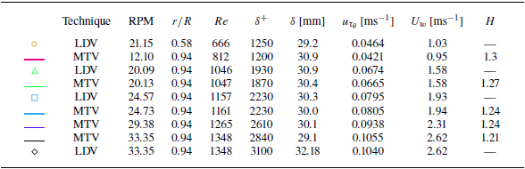
 r=750
r=750 mm
mm r/R=0.94
 R
R r=465
r=465 mm
mm δ+=1250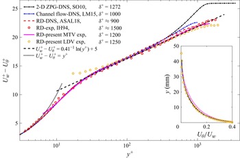
 δ+≈900
 δ+=1000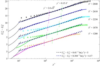
 δ+
δ+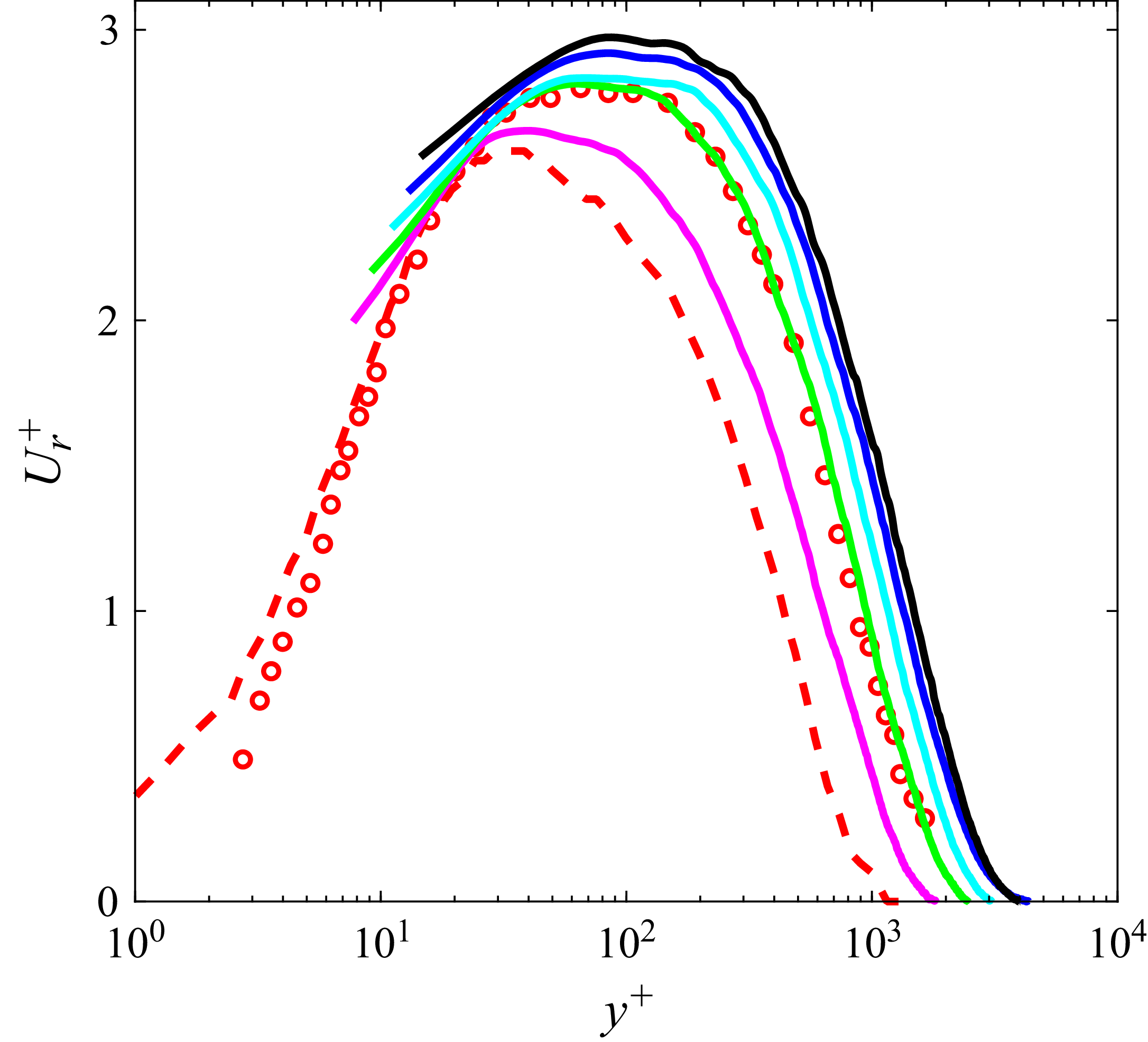
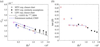
 Re2
Re2
 Uw
Uw U∞
U∞ δ+≈900
 δ+=1307,1571,
 1989
1989 δ+
δ+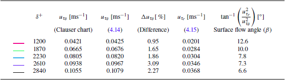
 r=750
r=750 mm
mm Δuτθ
Δuτθ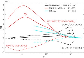
 x1
x1 θ1
θ1 x2
x2 θ2
θ2
 δ+=1307
 VF/TI
VF/TI y+
y+ δ+≈900
 δ+=1307
 r1
r1 r2
r2 Uθ+2/r+
 r2
r2
 x1
x1 θ1
θ1 x2
x2 θ2
θ2 δ+=2230
 δ+=1307
 δ+≈900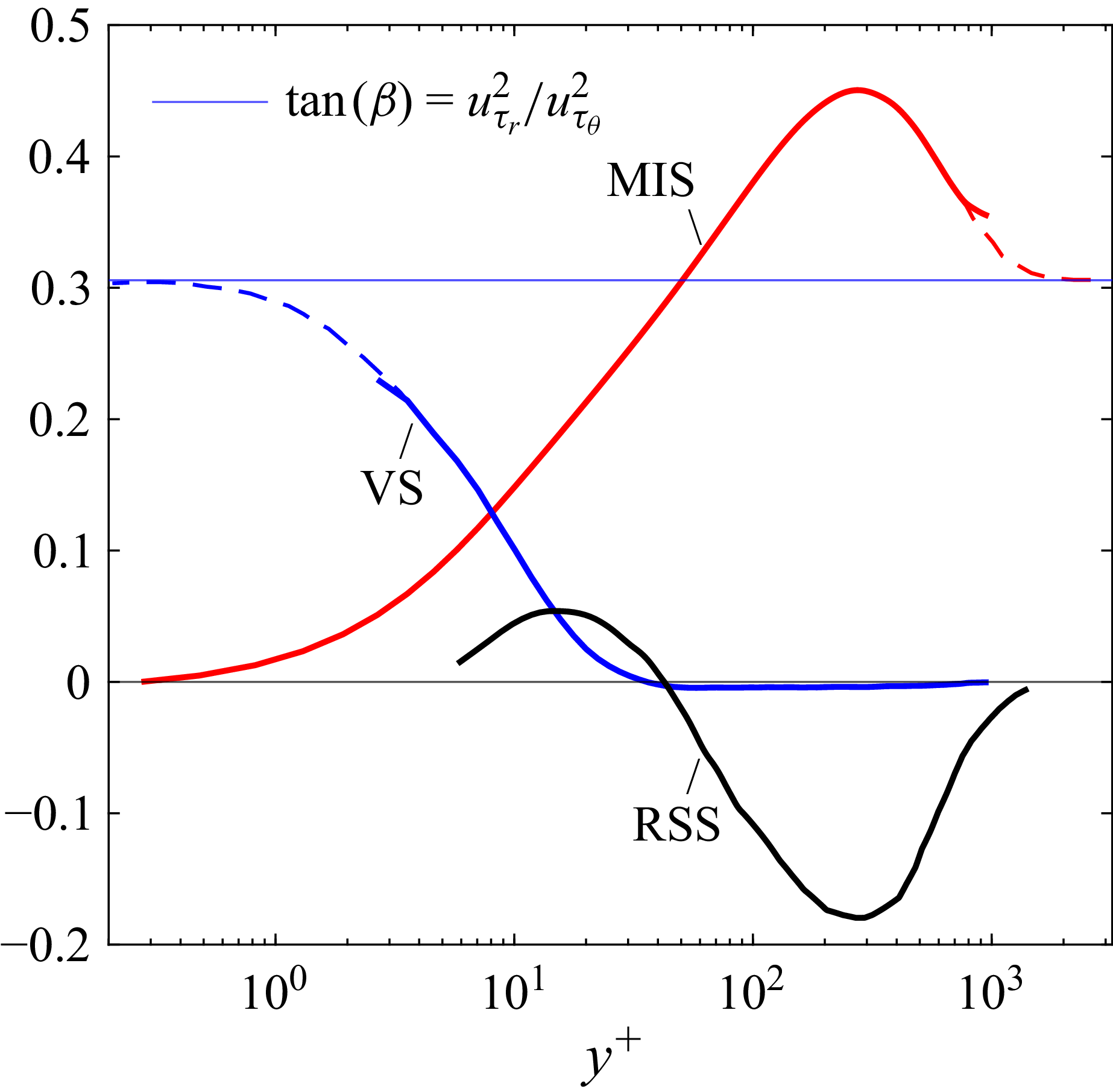
 −uruy¯+
 δ+≈900
 uτr2/uτθ2
 β=17∘
β=17∘ δ+≈900
 uθuy¯
uθuy¯ −uv¯
−uv¯ δ+=1930
 δ+=2400
 uθuy¯=−1/4.54ln(y+)+1.76
 δ+=590
 MIo
MIo TIo
TIo VFo
VFo δ+=1307
 VFo/TIo
 y/δ
y/δ δ+≈900
 δ+=1307
 Open access

