

1. Introduction
Laboratory experiments on dusty plasmas usually make use of solid particles in the size range between 100 nm and 20 ${\rm\mu}$
m diameter immersed in a gaseous plasma environment. In the plasma, the particles typically attain high negative charges due to the collection of plasma charge carriers (electrons and ions). This makes the dust particles a unique plasma species that is susceptible to various forces that are otherwise unimportant in plasmas. Moreover, the dust system usually is strongly coupled and this acts on very different time scales than electrons and ions. Indeed, the dust size, the interparticle distance and the time scales associated with the particle motion are ideally suited to study the dust by video microscopy (Bouchoule Reference Bouchoule1999; Shukla & Mamun Reference Shukla and Mamun2002; Melzer & Goree Reference Melzer, Goree, Hippler, Kersten, Schmidt and Schoenbach2008; Bonitz, Horing & Ludwig Reference Bonitz, Horing and Ludwig2010; Piel Reference Piel2010; Ivlev et al.
Reference Ivlev, Löwen, Morfill and Royall2012; Bonitz et al.
Reference Bonitz, Lopez, Becker and Thomsen2014). A wide variety of experiments have been performed on the structure and dynamics of these dust systems, see e.g. Shukla (Reference Shukla2001), Fortov, Vaulina & Petrov (Reference Fortov, Vaulina and Petrov2005), Bonitz et al. (Reference Bonitz, Ludwig, Baumgartner, Henning, Filinov, Block, Arp, Piel, Kding and Ivanov2008), Piel et al. (Reference Piel, Arp, Block, Pilch, Trottenberg, Käding, Melzer, Baumgartner, Henning and Bonitz2008), Shukla & Eliasson (Reference Shukla and Eliasson2009), Melzer et al. (Reference Melzer, Buttenschön, Miksch, Passvogel, Block, Arp and Piel2010), Merlino (Reference Merlino2014).
${\rm\mu}$
m diameter immersed in a gaseous plasma environment. In the plasma, the particles typically attain high negative charges due to the collection of plasma charge carriers (electrons and ions). This makes the dust particles a unique plasma species that is susceptible to various forces that are otherwise unimportant in plasmas. Moreover, the dust system usually is strongly coupled and this acts on very different time scales than electrons and ions. Indeed, the dust size, the interparticle distance and the time scales associated with the particle motion are ideally suited to study the dust by video microscopy (Bouchoule Reference Bouchoule1999; Shukla & Mamun Reference Shukla and Mamun2002; Melzer & Goree Reference Melzer, Goree, Hippler, Kersten, Schmidt and Schoenbach2008; Bonitz, Horing & Ludwig Reference Bonitz, Horing and Ludwig2010; Piel Reference Piel2010; Ivlev et al.
Reference Ivlev, Löwen, Morfill and Royall2012; Bonitz et al.
Reference Bonitz, Lopez, Becker and Thomsen2014). A wide variety of experiments have been performed on the structure and dynamics of these dust systems, see e.g. Shukla (Reference Shukla2001), Fortov, Vaulina & Petrov (Reference Fortov, Vaulina and Petrov2005), Bonitz et al. (Reference Bonitz, Ludwig, Baumgartner, Henning, Filinov, Block, Arp, Piel, Kding and Ivanov2008), Piel et al. (Reference Piel, Arp, Block, Pilch, Trottenberg, Käding, Melzer, Baumgartner, Henning and Bonitz2008), Shukla & Eliasson (Reference Shukla and Eliasson2009), Melzer et al. (Reference Melzer, Buttenschön, Miksch, Passvogel, Block, Arp and Piel2010), Merlino (Reference Merlino2014).
It is easy to see that it is necessary to measure the (three-dimensional) particle positions $\boldsymbol{r}_{i}$
of (each) particle
$\boldsymbol{r}_{i}$
of (each) particle $i$
to reveal the structure of a given particle arrangement. In the same way, one needs to know the velocities
$i$
to reveal the structure of a given particle arrangement. In the same way, one needs to know the velocities $\dot{\boldsymbol{r}}_{i}=\boldsymbol{v}_{i}={\rm\Delta}\boldsymbol{r}_{i}/{\rm\Delta}t$
and accelerations
$\dot{\boldsymbol{r}}_{i}=\boldsymbol{v}_{i}={\rm\Delta}\boldsymbol{r}_{i}/{\rm\Delta}t$
and accelerations $\ddot{\boldsymbol{r}}_{i}=\boldsymbol{a}_{i}={\rm\Delta}\boldsymbol{v}_{i}/{\rm\Delta}t$
to determine the particle dynamics. Hence, the equation of motion
$\ddot{\boldsymbol{r}}_{i}=\boldsymbol{a}_{i}={\rm\Delta}\boldsymbol{v}_{i}/{\rm\Delta}t$
to determine the particle dynamics. Hence, the equation of motion
 $$\begin{eqnarray}m\ddot{\boldsymbol{r}}_{i}+m{\it\beta}\dot{\boldsymbol{r}}_{i}=\boldsymbol{F}_{i}(\boldsymbol{r},\boldsymbol{v})\end{eqnarray}$$
becomes accessible to extract the relevant forces $\boldsymbol{F}_{i}$
on particle
$\boldsymbol{F}_{i}$
on particle $i$
. Here,
$i$
. Here, $m$
is the particle mass (which might or might not be known) and
$m$
is the particle mass (which might or might not be known) and ${\it\beta}$
is the corresponding (Epstein) friction coefficient (Epstein Reference Epstein1924; Liu et al.
Reference Liu, Goree, Nosenko and Boufendi2003).
${\it\beta}$
is the corresponding (Epstein) friction coefficient (Epstein Reference Epstein1924; Liu et al.
Reference Liu, Goree, Nosenko and Boufendi2003).
Here, video stereoscopy provides a very versatile and reliable technique to measure the individual three-dimensional (3-D) particle positions (and subsequently the particle velocities and accelerations in (1.1), where the time step ${\rm\Delta}t$
is just given by the frame rate of the cameras). In general, this technique requires multiple cameras (at least two) that observe the same volume under different angles. From the appearance of the particles under the different camera viewing angles, the three-dimensional particle position can then be reconstructed. In this article we will focus on stereoscopy. Other techniques that are able to retrieve 3-D particle positions include inline holography (Kroll, Block & Piel Reference Kroll, Block and Piel2008), colour-gradient methods (Annaratone et al.
Reference Annaratone, Antonova, Goldbeck, Thomas and Morfill2004), scanning video microscopy (Pieper, Goree & Quinn Reference Pieper, Goree and Quinn1996; Arp et al.
Reference Arp, Block, Piel and Melzer2004; Samsonov et al.
Reference Samsonov, Elsaesser, Edwards, Thomas and Morfill2008), light field imaging with plenoptic cameras (Hartmann, Donko & Donko Reference Hartmann, Donko and Donko2013) or tomographic-PIV (Williams Reference Williams2011) which, however, will not be reviewed here.
${\rm\Delta}t$
is just given by the frame rate of the cameras). In general, this technique requires multiple cameras (at least two) that observe the same volume under different angles. From the appearance of the particles under the different camera viewing angles, the three-dimensional particle position can then be reconstructed. In this article we will focus on stereoscopy. Other techniques that are able to retrieve 3-D particle positions include inline holography (Kroll, Block & Piel Reference Kroll, Block and Piel2008), colour-gradient methods (Annaratone et al.
Reference Annaratone, Antonova, Goldbeck, Thomas and Morfill2004), scanning video microscopy (Pieper, Goree & Quinn Reference Pieper, Goree and Quinn1996; Arp et al.
Reference Arp, Block, Piel and Melzer2004; Samsonov et al.
Reference Samsonov, Elsaesser, Edwards, Thomas and Morfill2008), light field imaging with plenoptic cameras (Hartmann, Donko & Donko Reference Hartmann, Donko and Donko2013) or tomographic-PIV (Williams Reference Williams2011) which, however, will not be reviewed here.
Stereoscopic set-up with 3 cameras in a non-rectangular geometry. The observation volume is imaged by two cameras from the side (via two mirrors) under a relative angle of about $26^{\circ }$
. The third camera looks from top (also via a mirror). The observation volume is inside the vacuum vessel (not shown).
$26^{\circ }$
. The third camera looks from top (also via a mirror). The observation volume is inside the vacuum vessel (not shown).

2. Diagnostics
The principal idea of stereoscopy is that a common observation volume is imaged by multiple cameras from different viewing angles. As an example, our stereoscopic camera set-up used for parabolic flight experiments (Buttenschön, Himpel & Melzer Reference Buttenschön, Himpel and Melzer2011; Himpel et al.
Reference Himpel, Killer, Buttenschön and Melzer2012, Reference Himpel, Killer, Melzer, Bockwoldt, Menzel and Piel2014) is shown in figure 1. For the parabolic flight experiments, three CCD cameras with $640\times 480$
pixels at a frame rate of approximately 200 frames per second (f.p.s.) are used. The cameras are fixed with respect to each other, but the entire system can be moved on two axes to freely position the observation volume within the discharge chamber. In our laboratory experiments, a stereoscopic system with three orthogonal cameras at megapixel resolution (
$640\times 480$
pixels at a frame rate of approximately 200 frames per second (f.p.s.) are used. The cameras are fixed with respect to each other, but the entire system can be moved on two axes to freely position the observation volume within the discharge chamber. In our laboratory experiments, a stereoscopic system with three orthogonal cameras at megapixel resolution ( $1280\times 1024$
) at 500 f.p.s. is installed (Käding et al.
Reference Käding, Block, Melzer, Piel, Kählert, Ludwig and Bonitz2008). In both cases, the cameras have to be synchronized to ensure that the frames of all cameras are recorded at the same instant.
$1280\times 1024$
) at 500 f.p.s. is installed (Käding et al.
Reference Käding, Block, Melzer, Piel, Kählert, Ludwig and Bonitz2008). In both cases, the cameras have to be synchronized to ensure that the frames of all cameras are recorded at the same instant.
To retrieve the 3-D particle positions, first of all the viewing geometry of the individual cameras has to be determined. The best results for our dusty plasma experiments with intense dust dynamics have been achieved when, second, the (two-dimensional) positions of the dust particles are identified and tracked through the image sequence in each camera individually. The next and most difficult step then is to identify corresponding particles in the different cameras. The problem here mainly lies in the fact that the particles in the camera images are indistinguishable. When this step has been accomplished one has the full 3-D particle positions at hand for the physical interpretation of structure and dynamics of the dust ensemble.
The individual steps together with the requirements and limitations will be discussed in the following.
2.1. Camera calibration
In a simple pinhole camera model (Hartley & Zisserman Reference Hartley and Zisserman2004) the viewing geometry of the camera can be described as follows (see Salvi, Armangué & Batlle (Reference Salvi, Armangué and Batlle2002) for camera calibration accuracy). A point in the world coordinate system $\unicode[STIX]{x1D648}=(X,Y,Z)^{\text{T}}$
is projected by the lens system onto a point
$\unicode[STIX]{x1D648}=(X,Y,Z)^{\text{T}}$
is projected by the lens system onto a point $(x_{p},y_{p})^{\text{T}}$
on the camera image plane by
$(x_{p},y_{p})^{\text{T}}$
on the camera image plane by
 $$\begin{eqnarray}\left(\begin{array}{@{}c@{}}x_{p}^{\prime }\\ y_{p}^{\prime }\\ z_{p}^{\prime }\end{array}\right)=\unicode[STIX]{x1D64B}\boldsymbol{\cdot }\left(\begin{array}{@{}c@{}}X\\ Y\\ Z\\ 1\end{array}\right)\quad \text{and}\quad \left(\begin{array}{@{}c@{}}x_{p}\\ y_{p}\end{array}\right)=\left(\begin{array}{@{}c@{}}x_{p}^{\prime }/z_{p}^{\prime }\\ y_{p}^{\prime }/z_{p}^{\prime }\end{array}\right),\end{eqnarray}$$
where $\unicode[STIX]{x1D64B}$
is the
$\unicode[STIX]{x1D64B}$
is the $3\times 4$
projection matrix. This projection matrix
$3\times 4$
projection matrix. This projection matrix
 $$\begin{eqnarray}\unicode[STIX]{x1D64B}=\unicode[STIX]{x1D646}\boldsymbol{\cdot }[\unicode[STIX]{x1D64D}\mid \boldsymbol{t}]\end{eqnarray}$$
contains the intrinsic $3\times 3$
camera matrix
$3\times 3$
camera matrix $\unicode[STIX]{x1D646}$
as well as the
$\unicode[STIX]{x1D646}$
as well as the $3\times 3$
rotation matrix
$3\times 3$
rotation matrix $\unicode[STIX]{x1D64D}$
and the translation vector
$\unicode[STIX]{x1D64D}$
and the translation vector $\boldsymbol{t}$
that describe the camera orientation and position with respect to the origin of the world coordinate system. The intrinsic camera matrix contains the camera-specific properties such as focal length
$\boldsymbol{t}$
that describe the camera orientation and position with respect to the origin of the world coordinate system. The intrinsic camera matrix contains the camera-specific properties such as focal length $f$
, principal point (image centre)
$f$
, principal point (image centre) $p$
and the skew
$p$
and the skew ${\it\alpha}$
(which generally is zero for modern cameras) and is then given by
${\it\alpha}$
(which generally is zero for modern cameras) and is then given by
 $$\begin{eqnarray}\unicode[STIX]{x1D646}=\left[\begin{array}{@{}ccc@{}}f_{x} & {\it\alpha} & p_{x}\\ 0 & f_{y} & p_{y}\\ 0 & 0 & 1\end{array}\right].\end{eqnarray}$$
From this it can be determined how a point in the real world is imaged onto the plane of the camera. In a stereoscopic camera system, this projection matrix $\unicode[STIX]{x1D64B}$
has to be determined for each camera individually.
$\unicode[STIX]{x1D64B}$
has to be determined for each camera individually.
An efficient way to determine the projection matrix for the cameras is to observe a calibration target with known properties simultaneously with all cameras. Wengert et al. (Reference Wengert, Reeff, Cattin and Székely2006) and Bouguet (Reference Bouguet2008) have developed Matlab toolboxes that allow us to reconstruct the projection matrices from the observation of a calibration target. Alternatively, ‘self-calibration’ routines can be applied (Svoboda, Martinec & Pajdla Reference Svoboda, Martinec and Pajdla2005) which yield camera projection models from observation of a small, easily detectable, bright spot. However, for measurements in calibrated real world units (e.g. mm) a calibration target with a known reference geometry is required.
(a–c) Images of the calibration target from the three cameras of the stereoscopic set-up (top view camera and the two side view cameras). One sees the dot calibration pattern with the two bars in the centre. For each view, processed data are overlaid, indicating the identified and indexed dots in the upper right quadrant. In the upper left quadrant only the identified dots without indexing are shown, indexing and identified dots have been omitted for the lower quadrants. (d) Shows the camera positions and orientations reconstructed from the different views of the target.

For our dusty plasma experiments, a calibration target with a pattern of dots of 0.5 mm diameter and a centre-to-centre distance of the dots of 1 mm has been found to be useful (see figure 2). In addition, according to Wengert et al. (Reference Wengert, Reeff, Cattin and Székely2006), the target has two perpendicular bars in the centre for unique identification of target orientation in the cameras. For further information on the target see Himpel, Buttenschön & Melzer (Reference Himpel, Buttenschön and Melzer2011), a different target and camera calibration concept can be found in Li et al. (Reference Li, Heng, Koser and Pollefeys2013).
This calibration target is now moved and rotated in the field of view of all cameras and simultaneous images for the different target positions or orientations have to be captured. Approximately 30–40 different target images per camera are sufficient to reliably determine the projection matrices $\unicode[STIX]{x1D64B}$
for each camera. For each image, the calibration dots are extracted using standard routines (Gaussian bandwidth filtering and successive position determination using the intensity moment method, see e.g. Feng, Goree & Liu (Reference Feng, Goree and Liu2007), Ivanov & Melzer (Reference Ivanov and Melzer2007)), the central bars are identified from their ratio of major to minor axis as well as their absolute area (Wengert et al.
Reference Wengert, Reeff, Cattin and Székely2006). The calibration dots are indexed by their position relative to the central bars. These coordinates are unique for every dot and are the same in all cameras and for all the different target orientations. This then allows to retrieve the line of sights of all cameras individually and the relative camera orientations, in short, the camera projection matrices (Bouguet Reference Bouguet2008).
$\unicode[STIX]{x1D64B}$
for each camera. For each image, the calibration dots are extracted using standard routines (Gaussian bandwidth filtering and successive position determination using the intensity moment method, see e.g. Feng, Goree & Liu (Reference Feng, Goree and Liu2007), Ivanov & Melzer (Reference Ivanov and Melzer2007)), the central bars are identified from their ratio of major to minor axis as well as their absolute area (Wengert et al.
Reference Wengert, Reeff, Cattin and Székely2006). The calibration dots are indexed by their position relative to the central bars. These coordinates are unique for every dot and are the same in all cameras and for all the different target orientations. This then allows to retrieve the line of sights of all cameras individually and the relative camera orientations, in short, the camera projection matrices (Bouguet Reference Bouguet2008).
The calibration target with the perpendicular orientation bars together with the Matlab toolboxes (Wengert et al. Reference Wengert, Reeff, Cattin and Székely2006; Bouguet Reference Bouguet2008) allow an automated analysis of the projection properties (Himpel et al. Reference Himpel, Buttenschön and Melzer2011). The camera calibration has to be performed in the actual experiment configuration (including mirrors etc.) and has to be updated each time the camera set-up is changed (adjustment of focus, adjustment of mirrors etc.). In a parabolic flight campaign, the calibration is performed before and after each flight day. The projection properties will be required to identify corresponding particles as described in § 2.3. An accurate calibration will return more reliable correspondences.
2.2. Particle position determination
In actual experiments, the particles are viewed with the different cameras in the stereoscopic set-up and the images are recorded on a computer. The first step in data analysis then is to identify the particles and their (2-D) positions in the camera images. This can be done using standard algorithms known from colloidal suspensions or from dusty plasmas, see e.g. Crocker & Grier (Reference Crocker and Grier1996), Feng et al. (Reference Feng, Goree and Liu2007), Ivanov & Melzer (Reference Ivanov and Melzer2007). Depending on image quality, first Sobel filtering or Gaussian bandwidth filtering of the image might be applied. Position determination can be done using intensity moment method or least-square Gaussian kernal fitting (Crocker & Grier Reference Crocker and Grier1996; Feng et al. Reference Feng, Goree and Liu2007; Ivanov & Melzer Reference Ivanov and Melzer2007). Such methods are usually able to determine particle positions with subpixel accuracy in the 2-D images when 5–10 pixels constitute a particle in the image. Problems occur when two or more particle projections overlap or are close to each other.
From our experience, we find it useful, as the next step, to track the particles from frame to frame in each camera separately. So, 2-D trajectories $(x_{p}(t),y_{p}(t))^{\text{T}}$
of particles in each camera are obtained. This is done by following each particle through the subsequent frames. Thereby, all particles that lie within a certain search radius in the subsequent frame are linked to the particle in the actual frame. Hence, a particle in the starting frame may constitute more than only a single possible trajectory through the next frames. Then, a cost function for all possible tracks of the start particle is computed. The cost of a trajectory increases with acceleration (both in change of speed and change of direction). The trajectory with lowest cost over the following 10 frames is chosen (Dalziel Reference Dalziel1992; Sbalzarini & Koumoutsakos Reference Sbalzarini and Koumoutsakos2005; Ouellette, Xu & Bodenschatz Reference Ouellette, Xu and Bodenschatz2006). This way, smoother trajectories are favoured.
$(x_{p}(t),y_{p}(t))^{\text{T}}$
of particles in each camera are obtained. This is done by following each particle through the subsequent frames. Thereby, all particles that lie within a certain search radius in the subsequent frame are linked to the particle in the actual frame. Hence, a particle in the starting frame may constitute more than only a single possible trajectory through the next frames. Then, a cost function for all possible tracks of the start particle is computed. The cost of a trajectory increases with acceleration (both in change of speed and change of direction). The trajectory with lowest cost over the following 10 frames is chosen (Dalziel Reference Dalziel1992; Sbalzarini & Koumoutsakos Reference Sbalzarini and Koumoutsakos2005; Ouellette, Xu & Bodenschatz Reference Ouellette, Xu and Bodenschatz2006). This way, smoother trajectories are favoured.
This 2-D particle tracking usually reliably works for up to 200 particles per frame (for a megapixel camera). When more particles are visible in an individual frame, a unique identification of 2-D particle trajectories becomes increasingly difficult. In general, this also limits the number of particles that should be visible in the 3-D observation volume to approximately 200 (see also § 3).
2.3. Identifying corresponding particles
To retrieve the 3-D particle positions it is necessary to identify corresponding particles in the different cameras (‘stereo matching’), i.e. we have to determine which particle in camera C $^{\prime }$
is the same particle that we have observed in camera C. As mentioned above, this task is quite difficult since the particles are indistinguishable. In standard techniques of computer vision one can exploit a number of image properties to identify correspondence, such as colour information, detection of edges or patterns etc. These do not work here since all the particles usually appear as very similar small patches of bright pixels against a dark background.
$^{\prime }$
is the same particle that we have observed in camera C. As mentioned above, this task is quite difficult since the particles are indistinguishable. In standard techniques of computer vision one can exploit a number of image properties to identify correspondence, such as colour information, detection of edges or patterns etc. These do not work here since all the particles usually appear as very similar small patches of bright pixels against a dark background.
This problem can be solved in two ways. When three (or more) cameras with good data quality are available, corresponding particles can be identified from the set of camera images taken at each instant by exploiting the epipolar line approach. When only two cameras can be used, then in the first step, we identify all possible corresponding particles in camera C $^{\prime }$
for a given particle in camera C using epipolar lines. Then, in the second step, we exploit the information from the 2-D trajectories
$^{\prime }$
for a given particle in camera C using epipolar lines. Then, in the second step, we exploit the information from the 2-D trajectories $(x_{p}(t),y_{p}(t))^{\text{T}}$
to pin down the single real corresponding particle.
$(x_{p}(t),y_{p}(t))^{\text{T}}$
to pin down the single real corresponding particle.
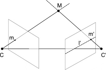
2.3.1. Correspondence analysis using epipolar lines
The possible corresponding particles are found from the epipolar line approach (Zhang Reference Zhang1998). In short, the epipolar line $l^{\prime }$
is the line of sight of the image point
$l^{\prime }$
is the line of sight of the image point $\boldsymbol{m}$
in the image plane of camera C of a 3-D point
$\boldsymbol{m}$
in the image plane of camera C of a 3-D point $\boldsymbol{M}$
as seen in the image plane of camera C
$\boldsymbol{M}$
as seen in the image plane of camera C $^{\prime }$
, as shown in figure 3. Here,
$^{\prime }$
, as shown in figure 3. Here, $\boldsymbol{m}$
is the 2-D position of a dust particle in the image of camera C and the point
$\boldsymbol{m}$
is the 2-D position of a dust particle in the image of camera C and the point $\boldsymbol{M}$
corresponds to the real world 3-D coordinate of the particle, which is to be determined. Now, the corresponding projection
$\boldsymbol{M}$
corresponds to the real world 3-D coordinate of the particle, which is to be determined. Now, the corresponding projection $\boldsymbol{m}^{\prime }$
of this point
$\boldsymbol{m}^{\prime }$
of this point $\boldsymbol{M}$
in the image plane of the second camera C
$\boldsymbol{M}$
in the image plane of the second camera C $^{\prime }$
has to lie on the epipolar line
$^{\prime }$
has to lie on the epipolar line $l^{\prime }$
.
$l^{\prime }$
.
Epipolar geometry for two cameras C and C $^{\prime }$
facing the point
$^{\prime }$
facing the point $\boldsymbol{M}$
. The epipolar line
$\boldsymbol{M}$
. The epipolar line $l^{\prime }$
is the projected line of sight from the image point
$l^{\prime }$
is the projected line of sight from the image point $\boldsymbol{m}$
to the 3-D point
$\boldsymbol{m}$
to the 3-D point $\boldsymbol{M}$
from camera C to C
$\boldsymbol{M}$
from camera C to C $^{\prime }$
.
$^{\prime }$
.
This condition can be formulated as
 $$\begin{eqnarray}\widetilde{\boldsymbol{m}}^{\prime T}\boldsymbol{\cdot }\unicode[STIX]{x1D641}\boldsymbol{\cdot }\widetilde{\boldsymbol{m}}=0,\end{eqnarray}$$
where $\widetilde{\boldsymbol{m}}=(m_{x},m_{y},1)^{\text{T}}$
and
$\widetilde{\boldsymbol{m}}=(m_{x},m_{y},1)^{\text{T}}$
and $\unicode[STIX]{x1D641}$
is the so called fundamental matrix
$\unicode[STIX]{x1D641}$
is the so called fundamental matrix
 $$\begin{eqnarray}\unicode[STIX]{x1D641}=\unicode[STIX]{x1D646}^{\prime -T}[\unicode[STIX]{x1D669}]_{\times }\unicode[STIX]{x1D64D}\unicode[STIX]{x1D646}^{-1},\end{eqnarray}$$
which can be constructed from the projection matrices of camera C and C $^{\prime }$
, see (2.2). Here,
$^{\prime }$
, see (2.2). Here, $[\unicode[STIX]{x1D669}]_{\times }$
is the antisymmetric matrix such that
$[\unicode[STIX]{x1D669}]_{\times }$
is the antisymmetric matrix such that $[\unicode[STIX]{x1D669}]_{\times }\boldsymbol{x}=\boldsymbol{t}\times \boldsymbol{x}$
.
$[\unicode[STIX]{x1D669}]_{\times }\boldsymbol{x}=\boldsymbol{t}\times \boldsymbol{x}$
.
Now, for a point $\boldsymbol{m}$
in camera C, all possible candidates
$\boldsymbol{m}$
in camera C, all possible candidates $\boldsymbol{m}^{\prime }$
lying within a narrow stripe around the current epipolar line
$\boldsymbol{m}^{\prime }$
lying within a narrow stripe around the current epipolar line $l^{\prime }$
are taken as the possible corresponding particles to the particle with image point
$l^{\prime }$
are taken as the possible corresponding particles to the particle with image point $\boldsymbol{m}$
. Empirically, the stripe width around the epipolar line is chosen to be approximately 1 pixel in our case, see figure 4.
$\boldsymbol{m}$
. Empirically, the stripe width around the epipolar line is chosen to be approximately 1 pixel in our case, see figure 4.
The figure shows a snapshot of a dust particle cloud from the three cameras of our stereoscopic set-up. In the left camera, a particle $a$
is chosen and the corresponding epipolar line
$a$
is chosen and the corresponding epipolar line $l_{a}^{\prime }$
in the right camera is calculated. In this case, there are 4 particles
$l_{a}^{\prime }$
in the right camera is calculated. In this case, there are 4 particles $a^{\prime }$
to
$a^{\prime }$
to $d^{\prime }$
in the right camera that have a small distance to the epipolar line and, thus, are possible corresponding particles to particle
$d^{\prime }$
in the right camera that have a small distance to the epipolar line and, thus, are possible corresponding particles to particle $a$
. When a third camera is present (top camera) the epipolar line
$a$
. When a third camera is present (top camera) the epipolar line $l_{a}^{\prime \prime }$
of particle
$l_{a}^{\prime \prime }$
of particle $a$
in the top camera can be calculated as well as the epipolar lines of the particles
$a$
in the top camera can be calculated as well as the epipolar lines of the particles $a^{\prime }$
to
$a^{\prime }$
to $d^{\prime }$
of the right camera. Now, it is checked whether there is a particle in the top camera that is close to the epipolar line
$d^{\prime }$
of the right camera. Now, it is checked whether there is a particle in the top camera that is close to the epipolar line $l_{a}^{\prime \prime }$
of particle
$l_{a}^{\prime \prime }$
of particle $a$
from the left camera and either of the epipolar lines of the possible candidates
$a$
from the left camera and either of the epipolar lines of the possible candidates $a^{\prime }$
to
$a^{\prime }$
to $d^{\prime }$
from the right camera. Here, in the top camera, there is only a single particle that is close to both the epipolar line
$d^{\prime }$
from the right camera. Here, in the top camera, there is only a single particle that is close to both the epipolar line $l_{a}^{\prime \prime }$
of particle
$l_{a}^{\prime \prime }$
of particle $a$
and, in this case, the epipolar line of particle
$a$
and, in this case, the epipolar line of particle $a^{\prime }$
(the epipolar lines
$a^{\prime }$
(the epipolar lines $l_{a}^{\prime \prime }$
of particle
$l_{a}^{\prime \prime }$
of particle $a$
and
$a$
and $l_{a^{\prime }}^{\prime \prime }$
of particle
$l_{a^{\prime }}^{\prime \prime }$
of particle $a^{\prime }$
are shown). Hence, here, a unique correspondence is found between particle
$a^{\prime }$
are shown). Hence, here, a unique correspondence is found between particle $a$
in the left camera,
$a$
in the left camera, $a^{\prime }$
in the right camera and
$a^{\prime }$
in the right camera and $a^{\prime \prime }$
in the top camera from a single snapshot.
$a^{\prime \prime }$
in the top camera from a single snapshot.
(a–c) Snapshot of a dust particle cloud from the three cameras of our stereoscopic set-up together with epipolar lines to check for particle correspondences (the raw images are inverted: particles appear dark on a light background). See text for details. (d) Deviation of the particles $a^{\prime }$
to
$a^{\prime }$
to $d^{\prime }$
from the (time dependent) epipolar line
$d^{\prime }$
from the (time dependent) epipolar line $l_{a}^{\prime }$
over several frames. Note the logarithmic axis scaling.
$l_{a}^{\prime }$
over several frames. Note the logarithmic axis scaling.

2.3.2. Correspondence analysis using trajectories
When a third camera is not available or the epipolar line criterion does not uniquely define particle correspondences, the dynamic information of the particle motion in camera C and C $^{\prime }$
can be exploited. From the tracking we have the 2-D trajectory of the chosen particle
$^{\prime }$
can be exploited. From the tracking we have the 2-D trajectory of the chosen particle $a$
in the left camera C
$a$
in the left camera C $(x_{a}^{C}(t),y_{a}^{C}(t))^{\text{T}}$
as well as the trajectories of the possible correspondences in camera C
$(x_{a}^{C}(t),y_{a}^{C}(t))^{\text{T}}$
as well as the trajectories of the possible correspondences in camera C $^{\prime }$ $(x_{p^{\prime }}^{C^{\prime }}(t),y_{p^{\prime }}^{C^{\prime }}(t))^{\text{T}}$
. It is then checked how far each possible correspondence in camera C
$(x_{p^{\prime }}^{C^{\prime }}(t),y_{p^{\prime }}^{C^{\prime }}(t))^{\text{T}}$
. It is then checked how far each possible correspondence in camera C $^{\prime }$
moves away over time from the (time dependent) epipolar line of particle
$^{\prime }$
moves away over time from the (time dependent) epipolar line of particle $a$
. For a real corresponding particle, the deviation of its 2-D particle position from the epipolar line is found to be less than approximately 1 pixel throughout the entire trajectory, see figure 4(d). It can be clearly seen that only the corresponding particle
$a$
. For a real corresponding particle, the deviation of its 2-D particle position from the epipolar line is found to be less than approximately 1 pixel throughout the entire trajectory, see figure 4(d). It can be clearly seen that only the corresponding particle $a^{\prime }$
stays close to the projected epipolar line whereas the others (
$a^{\prime }$
stays close to the projected epipolar line whereas the others ( $b^{\prime }$
to
$b^{\prime }$
to $d^{\prime }$
) develop much larger excursions.
$d^{\prime }$
) develop much larger excursions.
In our analysis the matching trajectories must have a minimum length of 50–100 frames. The advantage of this procedure is that the identified particle pairs are reliable corresponding particles. The disadvantage is that, due to the restrictions, a number of matching particles are not further considered. This happens mainly when the 2-D trajectories are not correctly determined over their temporal evolution. Nevertheless, in typical parabolic flight experiments we can identify several hundred reliable 3-D trajectories with a minimum length of 100 frames in a sequence of 1500 frames.
2.4. Three-dimensional trajectories, velocities and accelerations
Having identified the particle correspondences, the 3-D position is determined from triangulation. An optimized triangulation procedure according to Hartley & Sturm (Reference Hartley and Sturm1997) is used here. Because the approach is specially designed for triangulation with two cameras, there are three pairwise triangulations possible within a set of three cameras. We take the mean location of the three pairwise triangulations as the final particle position. The variance of each pairwise triangulation is called the triangulation error. The triangulation error results from the error in the projection matrices and camera vibrations as well as the 2-D particle position error. In our set-up, the triangulation error is usually of the order of $10~{\rm\mu}$
m when a 2-D particle position error of approximately 0.5 pixel is assumed.
$10~{\rm\mu}$
m when a 2-D particle position error of approximately 0.5 pixel is assumed.
Quite often, overlapping particle images will occur. Nevertheless, 3-D trajectories can still be reliably reconstructed for particles that have overlapping images in one camera, but not the other(s). More cameras help in minimizing the problems with overlapping images.
The stereoscopic algorithm hence determines the 3-D particle positions $\boldsymbol{r}_{i}(t)$
over time. As mentioned above, the particle velocities
$\boldsymbol{r}_{i}(t)$
over time. As mentioned above, the particle velocities $\boldsymbol{v}_{i}={\rm\Delta}\boldsymbol{r}_{i}/{\rm\Delta}t$
can then directly be determined (with
$\boldsymbol{v}_{i}={\rm\Delta}\boldsymbol{r}_{i}/{\rm\Delta}t$
can then directly be determined (with ${\rm\Delta}t$
being the time between successive video frames, i.e.
${\rm\Delta}t$
being the time between successive video frames, i.e. ${\rm\Delta}t$
is the inverse frame rate).
${\rm\Delta}t$
is the inverse frame rate).
However, due to uncertainties in the accuracy of the 3-D particle position, the 3-D trajectory is quite ‘noisy’ which makes it difficult to determine the velocity directly. Therefore, we found it useful first to smooth the original position data by a Savitzky–Golay filter (Savitzky & Golay Reference Savitzky and Golay1964) (in many cases a second-degree polynomial with a window width of nine frames has been used, see e.g. Buttenschön et al. (Reference Buttenschön, Himpel and Melzer2011)). From the smoothed position data, the difference quotient is computed to obtain the particle velocities $\boldsymbol{v}_{i}={\rm\Delta}\boldsymbol{r}_{i}/{\rm\Delta}t$
. For the particle acceleration, the velocity data are Savitzky–Golay smoothed again and used for computing the second difference quotient
$\boldsymbol{v}_{i}={\rm\Delta}\boldsymbol{r}_{i}/{\rm\Delta}t$
. For the particle acceleration, the velocity data are Savitzky–Golay smoothed again and used for computing the second difference quotient $\boldsymbol{a}_{i}={\rm\Delta}\boldsymbol{v}_{i}/{\rm\Delta}t$
.
$\boldsymbol{a}_{i}={\rm\Delta}\boldsymbol{v}_{i}/{\rm\Delta}t$
.
2.5. Algorithm
The determination of the 3-D particle positions from the stereoscopic camera images can be summarized in the following ‘algorithm’:
-
(1) Calibrate all cameras with the calibration target and compute the projection matrix $\unicode[STIX]{x1D64B}$
including the camera matrix
$\unicode[STIX]{x1D646}$
, rotation matrix
$\unicode[STIX]{x1D64D}$
and translation vector
$\boldsymbol{t}$
for all cameras.
$\unicode[STIX]{x1D64B}$
including the camera matrix
$\unicode[STIX]{x1D646}$
, rotation matrix
$\unicode[STIX]{x1D64D}$
and translation vector
$\boldsymbol{t}$
for all cameras. -
(2) Determine the 2-D particle positions and particle trajectories in the recorded images for each camera separately retrieving the 2-D trajectories
$(x_{p}^{C}(t),y_{p}^{C}(t))^{\text{T}}$
of the particles in all cameras. -
(3) Pick a particle
$p$
in camera C. -
(4) Determine its epipolar line
$l_{p}^{\prime }$
in camera C
$^{\prime }$
using (2.4). -
(5) Determine the possible corresponding particles
$p^{\prime }$
in C
$^{\prime }$
within a narrow stripe around the epipolar line
$l_{p}^{\prime }$
. -
(6)
-
(i) When three or more cameras are available: pin down the correspondences
$p$
and
$p^{\prime }$
by comparing the epipolar line criterion in the other camera(s). -
(ii) When only two cameras are available: calculate the distance of the possible correspondences
$p^{\prime }$
from the (time dependent) epipolar line of particle
$p$
. A corresponding particle
$p^{\prime }$
should not deviate by more than approximately 1 pixel from the epipolar line over 50 or so frames.
-
-
(7) Determine the 3-D position/3-D trajectory from the corresponding pair
$p$
and
$p^{\prime }$
from triangulation. -
(8) Return to step 3 for next particle
$p$
.


2.6. Requirements, conditions and limitations
From the above described stereoscopic reconstruction techniques the following requirements, conditions and limitations follow for successful application of stereoscopy:
-
(i) Two or more synchronized cameras with a common observation volume are required.
-
(ii) Stable, vibration-free mounting of all cameras is necessary.
-
(iii) Homogeneous illumination of the dust particles in the observation volume increases image quality and hence particle determination.
-
(iv) Larger angular distance between the cameras (the best is 90
$^{\circ }$
) improves triangulation accuracy. -
(v) A successful 3-D reconstruction of particle positions is possible when up to approximately 200 particles are visible in each camera (for a megapixel camera, see § 2.2).
-
(vi) In dense particle clouds, the visible particle number density can be decreased using fluorescent tracer particles (see § 3).
-
(vii) Correspondence analysis becomes increasingly difficult the more particles are found close to an epipolar line.

3. Example of measurement
As an example, we now discuss measurements of the microscopic particle motion in a dust-density wave (DDW) under weightlessness. DDWs are compressional and rarefactive waves of the dust component excited by an ion flow through the dust ensemble (Barkan, Merlino & D’Angelo Reference Barkan, Merlino and D’Angelo1995; Prabhakara & Tanna Reference Prabhakara and Tanna1996; Khrapak et al. Reference Khrapak, Samsonov, Morfill, Thomas, Yaroshenko, Rothermel, Hagl, Fortov, Nefedov and Molotkov2003; Schwabe et al. Reference Schwabe, Rubin-Zuzic, Zhdanov, Thomas and Morfill2007; Hou & Piel Reference Hou and Piel2008; Merlino Reference Merlino2009; Thomas Reference Thomas2009; Arp et al. Reference Arp, Caliebe, Menzel, Piel and Goree2010; Flanagan & Goree Reference Flanagan and Goree2010; Menzel et al. Reference Menzel, Arp, Caliebe and Piel2010; Himpel et al. Reference Himpel, Killer, Melzer, Bockwoldt, Menzel and Piel2014; Williams Reference Williams2014). These waves have frequencies of the order of 10 Hz and wave speeds of the order of a few centimetres per second. These waves are very prominent features in volume-filling dusty plasmas, see e.g. figure 5, they feature very strong density modulation between the wave crest and the wave trough.
Snapshot of a dust cloud with a DDW propagating from the dust-free central region (the ‘void’) to the boundaries of the dust cloud. Here, the particles are illuminated by an expanded laser sheet as well as by the smaller homogeneous beam of the illumination laser of the stereoscopic system. The volume imaged by the stereoscopic cameras is indicated by the dashed box. The illumination laser of the stereoscopy passes through the observation volume. The experimental data of the DDW have been measured in a different experiment run in the region indicated by the solid box. There, the wave propagation direction is indicated by the arrow and denoted as the $z$
-direction.
$z$
-direction.

Recently, the microphysics of particle motions in the crests and troughs, as well as the trapping of particles in the wave crest, have been of interest (Hou & Piel Reference Hou and Piel2008; Teng et al. Reference Teng, Chang, Tseng and I2009; Chang, Teng & I Reference Chang, Teng and I2012; Himpel et al. Reference Himpel, Killer, Melzer, Bockwoldt, Menzel and Piel2014). Since the observation of a 2-D slice of the dust can only give a limited view on the particle dynamics, it is beneficial to measure the 3-D particle motion. This has been done using our stereoscopic set-up shown in figure 1.
The experiments have been performed on a parabolic flight campaign during 2013 in Bordeaux, France. An argon plasma is produced in a capacitively coupled rf parallel-plate discharge. The discharge gap in the plasma chamber (IMPF-K2, (Klindworth, Arp & Piel Reference Klindworth, Arp and Piel2006)) is 3 cm. The discharge was operated with an rf-power of 3 W at a gas pressure of 20 Pa. The electrodes have a diameter of 8 cm. The dust particles in this experiment are melamine–formaldehyde (MF) microspheres with a diameter of 6.8 ${\rm\mu}$
m. The ion-excited DDWs then appear above a critical dust density (Menzel, Arp & Piel Reference Menzel, Arp and Piel2011).
${\rm\mu}$
m. The ion-excited DDWs then appear above a critical dust density (Menzel, Arp & Piel Reference Menzel, Arp and Piel2011).
To further reduce the number of visible particles in the observation volume of the stereoscopic cameras (see § 2.2) we have added to the ‘standard’ MF particles a small fraction of approximately 1–2 % of Rhodamine-B-doped fluorescent MF particles of the same mass and size. When illuminated by a $\text{Nd}:\text{YAG}$
laser at 532 nm these particles show a fluorescence around 590 nm. By using bandpass filters for wavelengths from 549 to 635 nm in front of the camera lenses we only observe the small number of fluorescent particles as tracer particles in our cameras (see Himpel et al. (Reference Himpel, Killer, Buttenschön and Melzer2012, Reference Himpel, Killer, Melzer, Bockwoldt, Menzel and Piel2014) for details). Figure 6 shows a snapshot of the fluorescent tracer particles inside a DDW as seen by the three stereoscopic cameras. In each camera approximately 50 particles are visible in the fluorescent light. The field of view was chosen to achieve single-particle resolution on the one hand, and to capture collective wave motion on the other. The density of visible (fluorescent) particles then is approximately 600 cm
$\text{Nd}:\text{YAG}$
laser at 532 nm these particles show a fluorescence around 590 nm. By using bandpass filters for wavelengths from 549 to 635 nm in front of the camera lenses we only observe the small number of fluorescent particles as tracer particles in our cameras (see Himpel et al. (Reference Himpel, Killer, Buttenschön and Melzer2012, Reference Himpel, Killer, Melzer, Bockwoldt, Menzel and Piel2014) for details). Figure 6 shows a snapshot of the fluorescent tracer particles inside a DDW as seen by the three stereoscopic cameras. In each camera approximately 50 particles are visible in the fluorescent light. The field of view was chosen to achieve single-particle resolution on the one hand, and to capture collective wave motion on the other. The density of visible (fluorescent) particles then is approximately 600 cm $^{-3}$
, which corresponds to a total particle density of roughly
$^{-3}$
, which corresponds to a total particle density of roughly $4\times 10^{4}~\text{ cm}^{-3}$
since the fluorescent particles constitute only 1–2 % of all particles.
$4\times 10^{4}~\text{ cm}^{-3}$
since the fluorescent particles constitute only 1–2 % of all particles.
Raw images of the particles in fluorescent light in the three stereoscopic cameras (here, for better recognition in the publication, a ‘dilate’ filter has been applied to the images using image processing tools). Also, the approximate region illuminated by the laser in the focal range is indicated by the lines. The images are $640\times 480$
pixels corresponding to approximately to
$640\times 480$
pixels corresponding to approximately to $8~\text{ mm}\times 6~\text{ mm}$
.
$8~\text{ mm}\times 6~\text{ mm}$
.

These images are taken from a single parabola of our parabolic flight campaign. The analysed image sequence had 1500 frames recorded at 180 f.p.s., hence covering 8.3 s of the 22 s of weightlessness during the parabola (at the beginning of the parabola the dust was injected and an equilibrium situation with self-excited DDWs had to develop before the sequence was taken).
(a) Trajectory of a single dust particle in the DDW. A clear oscillatory motion is seen. The instantaneous phase of the particle oscillations, as determined from a Hilbert transform, is colour coded. At oscillation maximum the phase angle is near zero (light/yellow colours) and at oscillation minimum it is near $\pm {\rm\pi}$
(dark/blue colours). (b) 3-D dust particle trajectories forming a DDW. The data are plotted in a moving reference frame accounting for the wave motion along the
$\pm {\rm\pi}$
(dark/blue colours). (b) 3-D dust particle trajectories forming a DDW. The data are plotted in a moving reference frame accounting for the wave motion along the $z$
-direction. Again, the colour indicates the instantaneous phase. (c) As (b), but averaged over the
$z$
-direction. Again, the colour indicates the instantaneous phase. (c) As (b), but averaged over the $y$
-direction. The arrows indicate the wave crests with phase angle near zero.
$y$
-direction. The arrows indicate the wave crests with phase angle near zero.

As described above, the 2-D positions of the particles have been identified in the individual cameras, their correspondences among the different cameras have been determined, and the 3-D trajectories of the particles have been derived. In total, 3-D trajectories of 233 particles with a minimum trajectory length of 75 frames have been obtained. Hence, it is observed that quite a large number of particle trajectories can be reconstructed. This even allows the derivation of statistical properties of the dust particle motion: as an example, the velocity distribution functions of the particles along the ( $z$
-direction) and perpendicular (
$z$
-direction) and perpendicular ( $x$
and
$x$
and $y$
-directions) to the wave propagation has been determined and analysed in Himpel et al. (Reference Himpel, Killer, Melzer, Bockwoldt, Menzel and Piel2014).
$y$
-directions) to the wave propagation has been determined and analysed in Himpel et al. (Reference Himpel, Killer, Melzer, Bockwoldt, Menzel and Piel2014).
Here, figure 7(a) shows the trajectory of a single particle during its oscillatory motion in the DDW. It is seen that the wave motion is mainly in the $z$
-direction (compare figure 5). For a more quantitative analysis the instantaneous phase of the particle oscillation has been determined from a Hilbert transform (see Menzel et al. (Reference Menzel, Arp and Piel2011), Killer et al. (Reference Killer, Himpel, Melzer, Bockwoldt, Menzel and Piel2014)) and is shown colour coded with the trajectory. As expected, it is found that near oscillation maximum the instantaneous phase is near zero whereas near oscillation minimum it shifts towards
$z$
-direction (compare figure 5). For a more quantitative analysis the instantaneous phase of the particle oscillation has been determined from a Hilbert transform (see Menzel et al. (Reference Menzel, Arp and Piel2011), Killer et al. (Reference Killer, Himpel, Melzer, Bockwoldt, Menzel and Piel2014)) and is shown colour coded with the trajectory. As expected, it is found that near oscillation maximum the instantaneous phase is near zero whereas near oscillation minimum it shifts towards $\pm {\rm\pi}$
.
$\pm {\rm\pi}$
.
We now investigate the full 3-D dust trajectories of all particles in a DDW. In figure 7(b) the trajectories, together with their instantaneous phases, are shown in a moving reference frame that accounts for the DDW propagation along the $z$
-direction, i.e. the
$z$
-direction, i.e. the $z$
-axis has been rescaled
$z$
-axis has been rescaled $z\rightarrow z-ct$
with the measured wave speed
$z\rightarrow z-ct$
with the measured wave speed $c={\it\omega}/k\approx 20~\text{ mm}~\text{ s}^{-1}$
. Also, a stroboscopic-like approach has been applied: with known wave period, the trajectories are mapped onto a single oscillation period of the DDW. For that purpose, from the times
$c={\it\omega}/k\approx 20~\text{ mm}~\text{ s}^{-1}$
. Also, a stroboscopic-like approach has been applied: with known wave period, the trajectories are mapped onto a single oscillation period of the DDW. For that purpose, from the times $t$
, entire multiples of the oscillation period
$t$
, entire multiples of the oscillation period $T=2{\rm\pi}/{\it\omega}=0.172$
s have been subtracted so that
$T=2{\rm\pi}/{\it\omega}=0.172$
s have been subtracted so that $0<t<T$
(Himpel et al.
Reference Himpel, Killer, Melzer, Bockwoldt, Menzel and Piel2014).
$0<t<T$
(Himpel et al.
Reference Himpel, Killer, Melzer, Bockwoldt, Menzel and Piel2014).
It is found that there are distinct stripes of fixed phases in this DDW representation indicating that here the DDW exhibits a coherent wave field. The DDW can be seen to extend approximately 3 wavelengths in the $z$
-direction whereas the phase is flat in the
$z$
-direction whereas the phase is flat in the $x$
and
$x$
and $y$
-directions, see also figure 7(c).
$y$
-directions, see also figure 7(c).
4. Future developments
Recently, other techniques have been developed to extract 3-D information of particle positions or velocities in dusty plasmas, namely light field imaging with plenoptic cameras (Hartmann et al. Reference Hartmann, Donko and Donko2013) or tomographic-PIV (Williams Reference Williams2011).
A light field image can be recorded by a so-called plenoptic camera using a microlens array directly in front of the camera chip. The lens array produces a large number of similar images of the object on the chip that usually has some to some ten megapixels. These multiple images then allow to compute refocused images representing different depth layers from the light field function and hence to determine the depth of the object, see e.g. (Levoy Reference Levoy2006) for details. Hartmann et al. (Reference Hartmann, Donko and Donko2013) have introduced this concept to dusty plasmas. It is very tempting and straightforward to combine stereoscopy with the imaging by plenoptic cameras.
Similarly, with tomographic-PIV a common observation volume is imaged by multiple cameras. After camera calibration, the intensity recorded along a line of sight is distributed over the observation volume which is divided into voxels. Typically, algebraic reconstruction techniques are employed to derive a ‘density’ distribution and from successive reconstructions a 3-D velocity field can be extracted by standard PIV adapted to three dimensions. Williams (Reference Williams2011) has applied this tomographic-PIV to dusty plasmas, recovering 3-D velocity fields. The general set-up and the camera calibration requirements seem to be quite comparable between tomographic-PIV and stereoscopy. In the case of high dust densities, tomographic-PIV is certainly better suited than stereoscopy since particle positions do not need to be determined. For low densities, stereoscopy allows us to determine individual trajectories. A cross-over from stereoscopy to tomographic-PIV certainly deserves to be studied.
5. Summary
We have presented the basic techniques for the application of stereoscopy to dusty plasmas. Stereoscopic methods allow to retrieve the full 3-D particle positions with high spatial and temporal resolution.
The underlying techniques have been demonstrated together with their requirements and limitations. As an example, stereoscopy has been applied to measure the microphysics of particles in a dust-density wave under the weightlessness conditions of a parabolic flight.
Acknowledgements
We gratefully acknowledge financial support from DFG under grant no. SFB-TR24, project A3 and from the German Aerospace Center DLR under 50 WM 1538.


