2.1. Geometry

The kinematic sketch of the H6A manipulator is shown in Fig. 1. The global frame of reference, ${\boldsymbol{{X}}}_0{\boldsymbol{{Y}}}_0{\boldsymbol{{Z}}}_0$ , is attached to the waist joint, ${\boldsymbol{{o}}}$ , which rotates about the ${\boldsymbol{{Z}}}_0$ axis. The robot manipulator is composed of a pair of 2-R “arms”, ${\boldsymbol{{s}}}_L{\boldsymbol{{e}}}_L$ - ${\boldsymbol{{e}}}_L\boldsymbol{{p}}_L$ on the left and ${\boldsymbol{{s}}}_R{\boldsymbol{{e}}}_R$ - ${\boldsymbol{{e}}}_R\boldsymbol{{p}}_R$ on the right, both of which are attached to the waist at a fixed offset $d_2$ from the centre of the waist, ${\boldsymbol{{o}}}$ . The left arm comprises an upper arm, ${\boldsymbol{{s}}}_L{\boldsymbol{{e}}}_L$ , of length $l_2$ and a forearm, ${\boldsymbol{{e}}}_L\boldsymbol{{p}}_L$ , of length $l_3$ . Similarly, the right arm consists of an upper arm, ${\boldsymbol{{s}}}_R{\boldsymbol{{e}}}_R$ , and a forearm, ${\boldsymbol{{e}}}_R\boldsymbol{{p}}_R$ , of lengths $l_2$ and $l_3$ , respectively. At the other end, the serial arms are connected together via a wrist assembly, $\boldsymbol{{p}}_L$ - ${\boldsymbol{{p}}}$ - $\boldsymbol{{p}}_R$ . The left arm is attached to the wrist assembly through a universal joint located at $\boldsymbol{{p}}_L$ . Likewise, a spherical at ${\boldsymbol{{p}}}_R$ joins the right arm and the wrist assembly. The wrist assembly itself consists of two links of length $l_w$ , which connect each arm to a rotary joint located at the wrist point, ${\boldsymbol{{p}}}$ . Additionally, an end-effector, ${\boldsymbol{{e}}}$ , is connected to the rotary joint at ${\boldsymbol{{p}}}$ , through an L-shaped link having proximal and distal arms of lengths $a_6$ and $d_7$ , respectively. Thereafter, the L-shaped link is joined to the link $\boldsymbol{{p}}_R\boldsymbol{{p}}$ at an angle $\kappa$ . While the closed loop ${\boldsymbol{{o}}}$ - ${\boldsymbol{{s}}}_L$ - ${\boldsymbol{{e}}}_L$ - $\boldsymbol{{p}}_L$ - ${\boldsymbol{{p}}}$ - $\boldsymbol{{p}}_R$ - ${\boldsymbol{{e}}}_R$ - ${\boldsymbol{{s}}}_R$ - ${\boldsymbol{{o}}}$ is responsible for the yaw and roll motions at the end-effector, a revolute actuator placed right before the end-effector is responsible for the pitch motion which is decoupled from the rest of the motions of the manipulator.

The waist joint at ${\boldsymbol{{o}}}$ , shoulder joints at ${\boldsymbol{{s}}}_L$ and ${\boldsymbol{{s}}}_R$ , elbow joints at ${\boldsymbol{{e}}}_L$ and ${\boldsymbol{{e}}}_R$ and the revolute joint situated before the end-effector, ${\boldsymbol{{e}}}$ , are active (i.e., actuated), and the corresponding joint angles are denoted by $\theta _1$ , $\theta _{2L}$ , $\theta _{2R}$ , $\theta _{3L}$ , $\theta _{3R}$ and $\theta _7$ , respectively. These joints account for the six-DoF of the end-effector.Footnote ⁴ On the other hand, the joints associated with the wrist assembly, that is, those located at ${\boldsymbol{{p}}}_L$ , $\boldsymbol{{p}}$ and ${\boldsymbol{{p}}}_R$ , respectively, are passive (i.e., unactuated), and the corresponding joint angles are $\{\phi _{4L}, \phi _{5L}\}$ , $\phi _{6L}$ and $\{\phi _{4R}, \phi _{5R}, \phi _{6R}\}$ , respectively. Figure 1 shows the references for all the pertinent joint angles. For instance, the angle $\theta _1$ is measured as the angle between $\mathbf{X}_0$ and $\boldsymbol{{x}}_1$ , measured about $\mathbf{Z}_0$ . Similarly, $\theta _7$ is the angle that $\boldsymbol{{x}}_e$ makes with (a line parallel to) $\boldsymbol{{x}}_{7L}$ . The close-ups of the wrist in Fig. 1 depict the framesFootnote ⁵ associated with the universal joint at $\boldsymbol{{p}}_L$ and spherical joint $\boldsymbol{{p}}_R$ . The intermediate frames at the spherical joint are omitted to avoid clutter. The rotation at the spherical joint $\boldsymbol{{p}}_R$ , between the frames $\boldsymbol{{x}}_{4R}\boldsymbol{{z}}_{4R}\boldsymbol{{y}}_{4R}$ and $\boldsymbol{{x}}_{7R}\boldsymbol{{y}}_{7R}\boldsymbol{{z}}_{7R}$ (the axes $\boldsymbol{{y}}_{4R},\boldsymbol{{y}}_{7R}$ being omitted in the figure) may be represented using the $\mathbf{Z}\mathbf{X}\mathbf{Z}$ convention of Euler angles as $\mathbf{R}_Z(\phi _{4R})\mathbf{R}_X(\phi _{5R})\mathbf{R}_Z(\phi _{6R}+\pi/2)$ . In summary, the H6A manipulator has a total of seven architecture parameters, namely $\{d_2, l_2, l_3, l_w, a_6, d_7, \kappa \}$ , and six actuated joints represented by the active angles, $\boldsymbol{\theta } = [\theta _1, \theta _{2L}, \theta _{2R}, \theta _{3L}, \theta _{3R}, \theta _7]^\top$ . In addition, there are six joints represented by the passive angles, $\boldsymbol{\phi } = [\phi _{4L}, \phi _{4R}, \phi _{5L}, \phi _{5R}, \phi _{6L}, \phi _{6R}]^\top$ . The left kinematic chain of the manipulator starts at the waist, ${\boldsymbol{{o}}}$ , and runs all the way to the end-effector, ${\boldsymbol{{e}}}$ , via the left elbow; it is designated as ${\boldsymbol{{o}}}\textrm{-}{\boldsymbol{{s}}}_L$ - ${\boldsymbol{{e}}}_L$ - $\boldsymbol{{p}}_L$ - ${\boldsymbol{{p}}}$ - ${\boldsymbol{{e}}}$ . Similarly, the right chain, running from ${\boldsymbol{{o}}}$ to $\boldsymbol{{p}}$ , is designated as ${{\boldsymbol{{o}}}}\textrm{-}{{\boldsymbol{{s}}}}_R\textrm{-}\boldsymbol{{p}}\textrm{-}{{\boldsymbol{{e}}}}_R\textrm{-}\boldsymbol{{p}}_R\textrm{-}\boldsymbol{{p}}$ . In order to keep the kinematic descriptions of these chains simple and generic, these are described via the DH parameters (see, e.g., ref. [Reference Ghosal1], pp. 43) owing primarily to the universal popularity of this system. The left and right chains are described in Tables I and II, respectively.Footnote ⁶ Further, from these tables, two sequences of $4\times 4$ homogeneous transformation matrices, namely ${}^{0}_{1}{{{\boldsymbol{{T}}}}},\dots,{}^{7}_{8}{{{\boldsymbol{{T}}}}}_L$ and ${}^{0}_{1}{{{\boldsymbol{{T}}}}},\dots,{}^{7}_{8}{{{\boldsymbol{{T}}}}}_R$ , are generated in a systematic manner, which are subsequently used in Section 2.2 to formulate the loop-closure equations of the manipulator.

Table I. DH parameters for the left chain of the H6A manipulator.

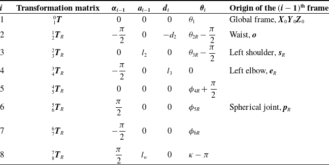
Table II. DH parameters for the right chain of the H6A manipulator.

It may be noted here that the architecture of the H6A is unique in the sense that it resembles two hands emanating separately from a single-DoF “waist”, which are brought back together at the wrist assembly. An additional and independently actuated link attached to the wrist assembly constitutes the final output. The remaining four-DoF appear in the portion of the manipulator where the two arms are not connected to each other. As such, it may be but natural to expect that these parts of the two arms, that is, ${{\boldsymbol{{s}}}}_L\textrm{-}{{\boldsymbol{{e}}}}_L\textrm{-}\boldsymbol{{p}}_L$ and ${{\boldsymbol{{s}}}}_R\textrm{-}{{\boldsymbol{{e}}}}_R\textrm{-}\boldsymbol{{p}}_R$ , should be identical in their architecture, inclusive of the manner at which they meet the wrist assembly. Indeed, this thought process seems to have led to the design of the manipulator H6AR, introduced in ref. [Reference Rao and Raju8], which preceded the manipulator H6A. However, the output DoF of the H6AR manipulator, based on its architecture, is seen to be five, that is, given its six actuators, the manipulator is redundantly actuated. The design of H6A eliminates this problem by replacing one of the two universal joints connecting the arms to the wrist assembly by a spherical joint (at $\boldsymbol{{p}}_R$ , to be specific), while retaining the symmetry in the rest of the architecture, as well as in the dimensions of the individual links.Footnote ⁷ Evidently, this asymmetric architecture leads to interesting kinematic behaviours, as may be seen in Section 4, in particular.

2.2. Loop-closure equations

The loop-closure equations are constraints which ensure that the manipulator maintains its kinematic integrity at every configuration. For the manipulator at hand, these equations are formulated by equating the pose of the wrist point $\boldsymbol{{p}}$ calculated through the left chain with that from the right. Hence, the transformation matrix ${}^{0}_{p}{{\boldsymbol{{T}}}}\in{\mathbb{SE}(3)}$ is determined as a concatenation of the matrices in constituting the second column of Table I using the left chain (see, e.g., ref. [Reference Ghosal1], pp. 48):

(1) \begin{align} &{}^{0}_{p}{{\boldsymbol{{T}}}} ={}^{0}_{1}{{\boldsymbol{{T}}}}{}^{1}_{2}{{\boldsymbol{{T}}}}_L\,{}^{2}_{3}{{\boldsymbol{{T}}}}_L\,{}^{3}_{4}{{\boldsymbol{{T}}}}_L\,{}^{4}_{5}{{\boldsymbol{{T}}}}_L\,{}^{5}_{6}{{\boldsymbol{{T}}}}_L\,{}^{6}_{7}{{\boldsymbol{{T}}}}_L. \end{align}

The matrix ${}^{0}_{p}{{\boldsymbol{{T}}}}$ may also be computed considering the right chain (refer to Table II):

(2) \begin{align} &{}^{0}_{p}{{\boldsymbol{{T}}}} ={}^{0}_{1}{{\boldsymbol{{T}}}}{}^{1}_{2}{{\boldsymbol{{T}}}}_R\,{}^{2}_{3}{{\boldsymbol{{T}}}}_R\,{}^{3}_{4}{{\boldsymbol{{T}}}}_R\,{}^{4}_{5}{{\boldsymbol{{T}}}}_R\,{}^{5}_{6}{{\boldsymbol{{T}}}}_R\,{}^{6}_{7}{{\boldsymbol{{T}}}}_R\,{}^{7}_{8}{{\boldsymbol{{T}}}}_R. \end{align}

Therefore, the loop-closure constraints are obtained by equating the expressions of ${}^{0}_{p}{{\boldsymbol{{T}}}}$ appearing in Eqs. (1) and (2) and eliminating the common factor, ${}^{0}_{1}{{\boldsymbol{{T}}}}$ , between them:

(3) \begin{align} &{}^{1}_{2}{{\boldsymbol{{T}}}}_L\,{}^{2}_{3}{{\boldsymbol{{T}}}}_L\,{}^{3}_{4}{{\boldsymbol{{T}}}}_L\,{}^{4}_{5}{{\boldsymbol{{T}}}}_L\,{}^{5}_{6}{{\boldsymbol{{T}}}}_L\,{}^{6}_{7}{{\boldsymbol{{T}}}}_L ={}^{1}_{2}{{\boldsymbol{{T}}}}_R\,{}^{2}_{3}{{\boldsymbol{{T}}}}_R\,{}^{3}_{4}{{\boldsymbol{{T}}}}_R\,{}^{4}_{5}{{\boldsymbol{{T}}}}_R\,{}^{5}_{6}{{\boldsymbol{{T}}}}_R\,{}^{6}_{7}{{\boldsymbol{{T}}}}_R\,{}^{7}_{8}{{\boldsymbol{{T}}}}_R. \end{align}

Equation (3) contains six independent scalar equations, which form the loop-closure equations of the manipulator. The six unknown passive joint angles, $\boldsymbol{\phi }$ , are solved in terms of the active joint angles, $\boldsymbol{\theta }$ , in the next section.

4.1. Elimination of $\theta _{2L}$

The constraint equations $\eta _1 = 0$ (see (19)) and $\eta _3 = 0$ (see (21)) are linear in the sine and cosine of $\theta _{2L}$ , respectively. Hence, the expressions of $\sin \theta _{2L}$ and $\cos \theta _{2L}$ are obtained from Eqs. (19) and (21):

(38) \begin{align} &\sin \theta _{2L}=\frac{\lambda _1(\theta _{\alpha _1}, \theta _{\gamma _7}, \psi _{6L}, \theta _{23L})}{l_2}, \quad \cos \theta _{2L}=\frac{\lambda _2(\theta _{\gamma _7}, \psi _{6L}, \theta _{23L})}{l_2},\ \textrm{since}\ l_2 \neq 0. \end{align}

In (38), the polynomials $\lambda _1$ and $\lambda _2$ are functions of the variables $\theta _{\alpha _1}, \theta _{\gamma _7}, \psi _{6L}$ and $\theta _{23L}$ . Substituting the expressions of $\sin \theta _{2L}$ and $\cos \theta _{2L}$ in the trigonometric identity $\cos ^2\theta _{2L} + \sin ^2\theta _{2L} = 1$ leads to a new equation in the remaining variables, namely $f(\theta _{\alpha _1}, \theta _{\gamma _7}, \psi _{6L}, \theta _{23L})= 0$ . The resulting elimination of $\theta _{2L}$ is depicted below schematically:Footnote ¹⁰

(39) \begin{align} &\begin{array}{cc}\left. \begin{array}{ll}{\eta _1(\theta _{\alpha _1}, \theta _{\gamma _7}, \psi _{6L}, \theta _{2L}, \theta _{23L}) = 0}\\[4pt] \eta _3(\theta _{\gamma _7}, \psi _{6L}, \theta _{2L}, \theta _{23L}) = 0\\ \end{array} \right ){\xrightarrow{\times \theta _{2L}}} \end{array} \begin{array}{cc} f(\theta _{\alpha _1}, \theta _{\gamma _7}, \psi _{6L}, \theta _{23L})= 0. \end{array} \end{align}

4.2. Elimination of $\phi _{5L}$

Equations $\eta _4=0$ and $\eta _5=0$ (see Eqs. (22) and (23)) are linear in the sine and cosine of $(\phi _{5L}+\psi _{6L})$ and hence may be represented as:

(40) \begin{align} &\eta _4\,{:\!=}\,i_1(\theta _{\alpha _1}) \cos (\phi _{5L}+\psi _{6L}) +j_1(\theta _{\alpha _1}, \theta _{\gamma _7}) \sin (\phi _{5L}+\psi _{6L}) + k_1(\theta _{23L})=0,\end{align}

(41) \begin{align} &\eta _5\,{:\!=}\,i_2 \cos (\phi _{5L}+\psi _{6L}) +j_2(\theta _{\gamma _7}) \sin (\phi _{5L}+\psi _{6L}) + k_2(\theta _{23L})=0, \end{align}

where the coefficients $i_i, j_i$ and $k_i$ are functions of the variables $\theta _{23L}, \psi _{6L}$ and $\theta _{\gamma _7}$ . The expressions of $\sin (\phi _{5L}+\psi _{6L})$ and $\cos (\phi _{5L}+\psi _{6L})$ are obtained from these equations and substituted in the trigonometric identity $\cos ^2(\phi _{5L}+\psi _{6L})+\sin ^2(\phi _{5L}+\psi _{6L})=1$ yielding:

(42) \begin{align} &n(\theta _{\alpha _1}, \theta _{\gamma _7}, \theta _{23L})\,{:\!=}\,\cos \theta _{23L} \sin \beta \sin \theta _{\gamma _7} - \sin \theta _{23L} (\!\cos \theta _{\gamma _7} \sin \theta _{\alpha _1} + \cos \beta \cos \theta _{\alpha _1} \sin \theta _{\gamma _7})=0. \end{align}

The above equation is obtained assumingFootnote ¹¹ that:

(43) \begin{align} &|ij|\,{:\!=}\,(i_1 j_2 - i_2 j_1) \neq 0. \end{align}

Equation (42) represents a kinematic constraint in the unknown variables $\theta _{\alpha _1}, \theta _{\gamma _7},$ and $\theta _{23L}$ . Furthermore, the conditions $i_1^2+j_1^2-k_1^2=0$ and $i_2^2+j_2^2-k_2^2=0$ cause repeated roots to satisfy (40) and (41), respectively. The details of this singularity are discussed in Case 1 in Section 6.2.

4.3. Elimination of $\theta _{23L}$

The constraint equations $n=0$ (see (42)) and $f=0$ (see (39)) are both linear in the sine and cosine of $\theta _{23L}$ and can be written explicitly in terms of $\cos \theta _{23L}$ and $\sin \theta _{23L}$ as:

(44) \begin{align} & n \,{:\!=}\, a_1(\theta _{\gamma _7}) \cos \theta _{23L} + b_1\left(\theta _{\gamma _7}, \theta _{\alpha _1}\right) \sin \theta _{23L} = 0,\end{align}

(45) \begin{align} & f \,{:\!=}\, a_2(\theta _{\gamma _7}, \psi _{6L}) \cos \theta _{23L} + b_2\left(\theta _{\gamma _7}, \theta _{\alpha _1}, \psi _{6L}\right) \sin \theta _{23L} + c_2\left(\theta _{\gamma _7}, \theta _{\alpha _1}, \psi _{6L}\right) = 0.\end{align}

As shown in Eqs. (44) and (45), the coefficients $a_i$ , $b_i$ and $c_i$ ( $i=1,2$ ) are functions of the unknown variables $\theta _{\alpha _1}, \psi _{6L}$ and $\theta _{\gamma _7}$ . Subsequently, the variable $\theta _{23L}$ is eliminated following the procedure described in Sections 4.1 and 4.2, leading to the equation:

(46) \begin{align} &{h_1\left(\theta _{\gamma _7}, \theta _{\alpha _1}, \psi _{6L}\right) \,{:\!=}\, c_2^2 \left(a_1^2 + b_1^2\right) - |ab|^2 = 0.} \end{align}

It is assumed in the above that:

(47) \begin{align} & |ab|\,{:\!=}\,\left(a_1 b_2 - a_2 b_1\right)\neq 0. \end{align}

Transferring $|ab|^2$ to the right-hand side of (46) and taking square roots of both the sides and rearranging, one obtains

(48) \begin{align} &h\left(\theta _{\gamma _7}, \theta _{\alpha _1}, \psi _{6L}\right) \,{:\!=}\, c_2 \mu - |ab| = 0, \, \textrm{where} \, \mu \left(\theta _{\gamma _7}, \theta _{\alpha _1}\right) \,{:\!=}\, \pm \sqrt{a_1^2 + b_1^2}. \end{align}

The size Footnote ¹² of the symbolic expression of $h$ is $13.080$ KB.

The identification of the form of (46) was made possible solely by the exact symbolic approach adopted in this work. It has allowed the reduction of this equation to (48), a step which is of critical importance in the symbolic computation scheme leading to the final univariate equation. It is a key enabler in permitting the computation to continue in the exact symbolic form, for two reasons: (a) it halves the degrees of the relevant variables appearing in (46) and (b) it helps in reducing the sizes of the expressions involved rather dramatically, without which the subsequent computations would have been rendered impractical (due to the demands on computational resources and time) or even infeasible. Consider, for instance, (53), which is derived below after a few steps. If it were to be derived directly from (46), it would have had a size of $6.110$ MB, which might have deterred subsequent symbolic computations. Also, the equation $p = 0$ would have been a quartic in the variable $c_6$ , making its elimination significantly more difficult in the computations that follow the derivation of (53). However, when the same equation is derived from (48), not only $p$ becomes a quadratic function of $c_6$ , as an expression, its size is reduced to only $19.232$ KB, that is, it is reduced by a factor greater than $300$ . As mentioned in Section 7, this and similar custom-developed techniques in symbolic computation allow the derivation of the key results in this paper.

It may be noted from (44) that $\theta _{23L}$ has finite number of values iff:

(49) \begin{align} & \mu \neq 0 \Rightarrow a_1^2+b_1^2 \neq 0. \end{align}

The condition $|ab|=0$ (see (47)), also causedFootnote ¹³ by $\mu =0$ (see (48)), results in a singularity of the manipulator. The details of the singularity are discussed in Case 2 in Section 6.2. Further, the condition $a_2^2+b_2^2-c_2^2=0$ leads to a double root of (45). The corresponding singularity is also studied in Section 6.2, in Case 3. It is worth mentioning that a merger of the solutions of the variable $\theta _{23L}$ leads to a repeated solution of the variable $\theta _{2L}$ as well.

4.4. Elimination of $\psi _{6L}$

The constraint equation $\eta _2=0$ (see (20)) is linear in the cosine and sine of $\psi _{6L}$ or, equivalently, linear in { $c_6$ , $s_6$ }, where $c_6=(a_6-l_w \cos \psi _{6L})$ and $s_6=(d_7 - l_w \sin \psi _{6L})$ . Therefore, for the sake of convenience, $\eta _2 = 0$ (see (20)) and $h=0$ (see (48)) are written in terms of { $c_6$ , $s_6$ } leading to the equations $g_1\left(\theta _{\gamma _7}, \theta _{\alpha _1}, c_6, s_6\right)=0$ and $g_2\left(\theta _{\gamma _7}, \theta _{\alpha _1}, c_6, s_6\right)=0$ , respectively:

(50) \begin{align} &\begin{array}{cc} \begin{array}{ll} \begin{aligned} &\eta _2\left(\theta _{\gamma _7}, \theta _{\alpha _1}, \psi _{6L}\right) = 0{\xrightarrow{\psi _{6L} \rightarrow c_6, s_6}} && g_1\left(\theta _{\gamma _7}, \theta _{\alpha _1}, c_6, s_6\right) = 0,\\ &h\left(\theta _{\gamma _7}, \theta _{\alpha _1}, \psi _{6L}\right) = 0{\xrightarrow{\psi _{6L} \rightarrow c_6, s_6}} && g_2\left(\theta _{\gamma _7}, \theta _{\alpha _1}, c_6, s_6\right) = 0.\\ \end{aligned} \end{array} \end{array} \end{align}

In the above, the symbol ‘ $\xrightarrow{\psi _{6L} \rightarrow c_6, s_6}$ ’ implies the absorption of the trigonometric variables of $\psi _{6L}$ into the algebraic variables $s_6$ and $c_6$ . Subsequently, the expression of $s_6$ is obtained in terms of $c_6$ from $g_1\left(\theta _{\gamma _7}, \theta _{\alpha _1}, c_6, s_6\right) = 0$ :Footnote ¹⁴

(51) \begin{align} &s_6 = \frac{1}{\sin \beta \sin \theta _{\alpha _1}} \zeta \left(\theta _{\gamma _7}, \theta _{\alpha _1}, c_6\right), \; \textrm{assuming} \;\; \sin \beta \sin \theta _{\alpha _1} \neq 0. \end{align}

Substituting $s_6$ from (51) in the modified trigonometric identity $(a_6-c_6)^2+(d_7-s_6)^2=l_w^2$ yields a quadratic equation in $c_6$ , denoted by $g\left(\theta _{\gamma _7}, \theta _{\alpha _1}, c_6\right)=0$ :

(52) \begin{align} &\begin{array}{cc}\left. \begin{array}{ll} g_1\left(\theta _{\gamma _7}, \theta _{\alpha _1}, c_6, s_6\right) = 0\\ \\[-8pt] (a_6 - c_6)^2+(d_7 - s_6)^2-l_w^2=0 \\ \end{array} \right ){\xrightarrow{\times s_6}} \end{array} \begin{array}{cc} g\left(\theta _{\gamma _7}, \theta _{\alpha _1}, c_6\right)=0. \end{array} \end{align}

Likewise, the expression of $s_6$ presented in (51) is substituted in $g_2=0$ (see (50)) to obtain a quadratic in $c_6$ of size $19.232$ KB, namely $p\left(\theta _{\gamma _7}, \theta _{\alpha _1}, c_6\right)=0$ :

(53) \begin{align} &\begin{array}{cc}\left. \begin{array}{ll} \begin{aligned} & g_1\left(\theta _{\gamma _7}, \theta _{\alpha _1}, c_6, s_6\right) = 0\\ \\[-8pt] & g_2\left(\theta _{\gamma _7}, \theta _{\alpha _1}, c_6, s_6\right) = 0\\ \end{aligned} \end{array} \right ){\xrightarrow{\times s_6}} \end{array} \begin{array}{cc} \begin{aligned} p\left(\theta _{\gamma _7}, \theta _{\alpha _1}, c_6\right)=0. \end{aligned} \end{array} \end{align}

Hereafter, the equations $g=0$ and $p=0$ may be represented as:

(54) \begin{align} &g\left(\theta _{\gamma _7}, \theta _{\alpha _1}, c_6\right)\,{:\!=}\,a_3 c_6^2 + b_3 c_6 + c_3=0, \end{align}

(55) \begin{align} &p\left(\theta _{\gamma _7}, \theta _{\alpha _1}, c_6\right)\,{:\!=}\,a_4 c_6^2 + b_4 c_6 + c_4=0, \end{align}

where the coefficients $a_i, b_i$ and $c_i$ ( $i=3,4$ ) are functions of the variables $\theta _{\gamma _7}$ and $\theta _{\alpha _1}$ . Simultaneous satisfaction of the conditions $b_3^2- 4a_3c_3= 0$ and $b_4^2-4 a_4 c_4=0$ causes the roots of Eqs. (54) and (55) to repeat. The corresponding singularity is discussed under Case 4 in Section 6.2. The resultantFootnote ¹⁵ of $p = 0$ and $g = 0$ with respect to $c_6$ eliminatesFootnote ¹⁶ the variable and leads to a new equation $q\left(\theta _{\gamma _7}, \theta _{\alpha _1}\right)=0$ of size $839.088$ KB:

(56) \begin{align} &\begin{array}{cc}\left. \begin{array}{ll} p\left(\theta _{\gamma _7}, \theta _{\alpha _1}, c_6\right) = 0 \\ \\[-8pt] g\left(\theta _{\gamma _7}, \theta _{\alpha _1}, c_6\right) = 0 \\ \end{array} \right ){\xrightarrow{\times c_6}} \end{array} \begin{array}{cc} q\left(\theta _{\gamma _7}, \theta _{\alpha _1}\right) = 0. \end{array} \end{align}

As noted before, the elimination of $c_6$ was greatly facilitated by the reduction of (46) to (48).

Continuing further, the function $q=0$ was simplified symbolically,Footnote ¹⁷ which afforded its factorisation in the following manner:

(57) \begin{align} &q\left(\theta _{\gamma _7}, \theta _{\alpha _1}\right) \,{:\!=}\, \mu ^3 \sin ^2\beta \sin ^2\theta _{\alpha _1} \delta \left(\theta _{\gamma _7}, \theta _{\alpha _1}\right) = 0, \end{align}

where $\delta \left(\theta _{\gamma _7}, \theta _{\alpha _1}\right)$ is a cubic polynomial in $\mu$ . Since it has already been assumed that $\mu \neq 0$ and $\sin \beta \sin \theta _{\alpha _1}\neq 0$ (in the context of Eqs. (49) and (51)), (57) reduces to $\delta \left(\theta _{\gamma _7}, \theta _{\alpha _1}\right)=0$ , which may be written as:

(58) \begin{align} &\delta \left(\theta _{\gamma _7}, \theta _{\alpha _1}\right) \,{:\!=}\, m_0 \mu ^3 + m_1 \mu ^2 + m_2 \mu + m_3 = 0. \end{align}

The coefficients in (58), namely $m_i$ , are also functions of the variables $\theta _{\gamma _7}$ and $\theta _{\alpha _1}$ . Since it is known (from (48)) that $\mu ^2 = a_1^2 + b_1^2$ , (58) is manipulated to derive its equivalent, cast in terms of $\mu ^2$ :

(59) \begin{align} &\delta _1\left(\theta _{\gamma _7}, \theta _{\alpha _1}\right) \,{:\!=}\, (m_0 \mu ^2 + m_2)^2 \mu ^2 - (m_1 \mu ^2 + m_3)^2 = 0. \end{align}

Direct substitution of the expressions of the coefficients $m_i$ and $\mu ^2$ in (59) leads to the following equation free of radicals:

(60) \begin{align} &\begin{array}{cc}\left. \begin{array}{ll} \delta _1\left(\theta _{\gamma _7}, \theta _{\alpha _1}\right) = 0\\ \\[-8pt] \mu ^2 - \left(a_1^2 + b_1^2\right) = 0 \\ \end{array} \right ){\xrightarrow{\times \mu ^2}} \end{array} \begin{array}{cc} r\left(\theta _{\gamma _7}, \theta _{\alpha _1}\right) = 0. \end{array} \end{align}

However, the size of $r\left(\theta _{\gamma _7}, \theta _{\alpha _1}\right)$ , even after rigorous simplification, stands at $216.140$ MB. It is reduced in the next step, before proceeding further.

4.5. Elimination of $\theta _{\gamma _7}$

The expression $r\left(\theta _{\gamma _7}, \theta _{\alpha _1}\right)$ turns out to be cubic in $\cos \theta _{\gamma _7}$ . However, using the identities:

(61) \begin{align} \cos ^{2m}\theta _{\alpha _1} = \left(1 - \sin ^2\theta _{\alpha _1}\right)^m, \quad m \in \mathbb{Z}^+, \end{align}

(60) is reduced to:

(62) \begin{align} r_l\left(\theta _{\gamma _7}, \theta _{\alpha _1}\right) = 0. \end{align}

The polynomial $r_l$ is linear in $\cos \theta _{\gamma _7}$ . Furthermore, this reduction results in fewer coefficients, which, upon symbolic simplification, shrink to the size of $89.311$ MB. It may be noted here that the equation $\eta _6=0$ (see (27)), is also linear in $\cos \theta _{\gamma _7}$ and $\sin \theta _{\gamma _7}$ , from which one can find $cos\theta _{\gamma _7}$ in terms of $\sin \theta _{\gamma _7}$ :Footnote ¹⁸

(63) \begin{align} \cos \theta _{\gamma _7} = &\frac{\nu \left(\theta _{\alpha _1}, \sin \theta _{\gamma _7}\right)}{(a_6 - l_w \cos \kappa )\cos \beta \sin \theta _{\alpha _1}},\;\textrm{assuming } \ (a_6 - l_w \cos \kappa )\cos \beta \sin \theta _{\alpha _1} \neq 0. \end{align}

In (63), $\nu \left(\theta _{\alpha _1}, \sin \theta _{\gamma _7}\right)$ is linear in $\cos \theta _{\alpha _1}$ , $\sin \theta _{\alpha _1}$ and $\sin \theta _{\gamma _7}$ . Substituting the expression of $\cos \theta _{\gamma _7}$ in (62) results in a sextic equation in $\sin \theta _{\gamma _7}$ , namely $u_1\left(\theta _{\alpha _1}, \sin \theta _{\gamma _7}\right)=0$ :

(64) \begin{align} &\begin{array}{cc}\left. \begin{array}{ll} \eta _6\left(\theta _{\gamma _7}, \theta _{\alpha _1}\right) = 0 \\ \\[-9pt] r_l\left(\theta _{\gamma _7}, \theta _{\alpha _1}\right) = 0 \\ \end{array} \right ){\xrightarrow{\times \cos \theta _{\gamma _7}}} \end{array} \begin{array}{cc} u_1\left(\theta _{\alpha _1}, \sin \theta _{\gamma _7}\right) = 0. \end{array} \end{align}

It may be noted here that the reduction of (60) to (62) is yet another improvisation in symbolic computation which has played a crucial role in the derivation of the inverse kinematic univariate (IKU) in its symbolic form. Specifically, if the equation $r = 0$ was used in (64) instead of $r_l= 0$ , the resulting size of $u_1$ would have been $191.635$ MB. However, due to the said reduction, the actual size turns out to be $79.873$ MB, which allows the computation to proceed further.

In the next step, the expression of $\cos \theta _{\gamma _7}$ (from (63)) is substituted in the trigonometric identity $\cos ^2\theta _{\gamma _7}+ \sin ^2\theta _{\gamma _7} = 1$ , to obtain a quadratic equation in $\sin \theta _{\gamma _7}$ , namely $u_2\left(\theta _{\alpha _1}, \sin \theta _{\gamma _7}\right) = 0$ :

(65) \begin{align} &\begin{array}{cc}\left. \begin{array}{ll} \eta _6\left(\theta _{\gamma _7}, \theta _{\alpha _1}\right) = 0 \\ \\[-6pt] \cos ^2\theta _{\gamma _7}+\sin ^2\theta _{\gamma _7} - 1 = 0 \\ \end{array} \right ){\xrightarrow{\times \cos \theta _{\gamma _7}}} \end{array} \begin{array}{cc} u_2\left(\theta _{\alpha _1}, \sin \theta _{\gamma _7}\right) = 0. \end{array} \end{align}

Eliminating $\sin \theta _{\gamma _7}$ between Eqs. (64) and (65) yields the univariate equation in $\theta _{\alpha _1}$ , that is, $u(\theta _{\alpha _1})= 0$ , which is of total degree $26$ in $\sin \theta _{\alpha _1}$ and $\cos \theta _{\alpha _1}$ :

(66) \begin{align} &\begin{array}{cc}\left. \begin{array}{ll} u_1\left(\theta _{\alpha _1}, \sin \theta _{\gamma _7}\right) = 0 \\ \\[-6pt] u_2\left(\theta _{\alpha _1}, \sin \theta _{\gamma _7}\right) = 0 \\ \end{array} \right ){\xrightarrow{\times \sin \theta _{\gamma _7}}} \end{array} \begin{array}{cc} u(\theta _{\alpha _1}) = 0. \end{array} \end{align}

Therefore, one may arrive at the final univariate polynomial from (66), as described in the next subsection. However, before that, a few special cases must be considered, for the sake of completeness.

It may be noted that repeated roots in the sextic equation $u_1=0$ (see (64)) and the quadratic equation $u_2=0$ (see (65)) cause the manipulator to encounter a singularity. The sextic $u_1= 0$ (see (64)) is a polynomial equation in $s_7 = \sin \theta _{\gamma _7}$ and its discriminant may be obtained as:

(67) \begin{align} \Delta _{1} = \operatorname{res}\left (u_1, \dfrac{\partial u_1}{\partial s_7}, s_7\right ). \end{align}

In (67), $\operatorname{res}(a(x),b(x),x)$ denotes the resultant of the polynomials $a(x)$ and $b(x)$ w.r.t. $x$ . Further, Equation (65) may be written as:

(68) \begin{align} &u_2\left(\theta _{\alpha _1}, \sin \theta _{\gamma _7}\right) \,{:\!=}\, a_5\;\sin ^2\theta _{\gamma _7} + b_5\;\sin \theta _{\gamma _7} + c_5 = 0. \end{align}

In (68), the coefficients $a_5, b_5$ and $c_5$ are functions of $\theta _{\alpha _1}$ alone. Hence, the manipulator encounters a singularity when the discriminants of Eqs. (64) and (65), that is, $\Delta _{1}$ (see (67)) and $b_5^2- 4a_5c_5$ (see (68)), respectively, vanish simultaneously. The corresponding singularity is studied as Case 5 in Section 6.2.

4.6. Derivation of the IKU equation

In the following, the total degree of the equation $u=0$ (66) in $\sin \theta _{\alpha _1}$ and $\cos \theta _{\alpha _1}$ is brought down from $26$ to $20$ through the identification and subsequent rejection of spurious factors, which are associated with singular solutions. Once again, this is an important step involving symbolic simplification and factorisation, without which the final univariate polynomial equation, that is, the IKU, would have been of degree 52, and not 40, as it is in (74).

The elimination process in (66) is simplified by rewriting $u_1=0$ and $u_2=0$ as polynomial equations in $\sin \theta _{\gamma _7}$ :

(69) \begin{align} u_1 &\,{:\!=}\, \;\tau (\theta _{\alpha _1}) u_{16} \sin ^6\theta _{\gamma _7} + u_{15} \sin ^5\theta _{\gamma _7} + u_{14} \sin ^4\theta _{\gamma _7} + u_{13} \sin ^3\theta _{\gamma _7\nonumber }\\[3pt] &\quad + u_{12} \sin ^2\theta _{\gamma _7} + u_{11} \sin \theta _{\gamma _7} + u_{10} = 0, \end{align}

(70) \begin{align} &u_2 \,{:\!=}\, \tau (\theta _{\alpha _1})\sin ^2\theta _{\gamma _7} + u_{21} \sin \theta _{\gamma _7} + u_{20} = 0. \end{align}

In the preceding equations, the coefficients $u_{ij}$ are functions of $\theta _{\alpha _1}$ ; also,

(71) \begin{align} &\tau (\theta _{\alpha _1})\,{:\!=}\,\cos ^2\theta _{\alpha _1} + \cos ^2\beta \sin ^2\theta _{\alpha _1}. \end{align}

Thus, the resulting equation $u(\theta _{\alpha _1}) = 0$ obtained by the elimination of $\sin \theta _{\gamma _7}$ from Eqs. (69) and (70) depends on $u_{ij}(\theta _{\alpha _1})$ and $\tau (\theta _{\alpha _1})$ , that is, ultimately, on $\theta _{\alpha _1}$ alone. It is interesting to note that $\tau (\theta _{\alpha _1})=0$ trivially satisfies (70) and therefore, $\tau (\theta _{\alpha _1})\neq 0$ for $\theta _{\gamma _7}$ to have finite number of values. Expressing $u(\theta _{\alpha _1}) = 0$ in terms of the coefficients $u_{ij}$ affords the advantage of yielding the factor $\tau ^2(\theta _{\alpha _1})$ without having to handle the large-sized expressions of $u_{ij}$ :

(72) \begin{align} u(\theta _{\alpha _1}) \,{:\!=}\, \tau ^2(\theta _{\alpha _1})w_1(\theta _{\alpha _1}) = 0, \end{align}

where $w_1(\theta _{\alpha _1})$ is a function of $u_{ij}$ . As the factor $\tau (\theta _{\alpha _1})$ appears in the leading coefficients of Eqs. (69) and (70), the manipulator encounters a singularity when $\tau (\theta _{\alpha _1})=0$ , which is described in Case 1 of Section 6.2. Therefore, in the non-singular cases, the relevant part of (72) is given by $w_1(\theta _{\alpha _1})=0$ . Subsequently, the actual expressions of the variables $u_{ij}$ are substituted in $w_1=0$ , along with the architecture parameters mentioned in Table III, which increases the size of $w_1=0$ significantly to $25.388$ MB even before its symbolic expansion, making further computation time-consuming and computationally complex. To overcome the aforementioned issues, the coefficients $u_{ij}$ are transformed to the respective monomial-based canonical (MBC) forms (see ref. [Reference Bandyopadhyay and Ghosal24], Section 3, for the details), treating $\sin \theta _{\gamma _7}$ and $\cos \theta _{\gamma _7}$ as algebraic variables. Consequently, substituting these expressions of the coefficients $u_{ij}$ in $w_1=0$ results in $w_2(\!\sin \theta _{\alpha _1}$ , $\cos \theta _{\alpha _1})= 0$ , which is a polynomial of total degree $22$ in $\sin \theta _{\alpha _1}$ and $\cos \theta _{\alpha _1}$ . The maximum degrees of $\cos \theta _{\alpha _1}$ and $\sin \theta _{\alpha _1}$ in $w_2(\theta _{\alpha _1})$ are 4 and 22, respectively. Subsequently, $w_2$ is reduced to a linear function of $\cos \theta _{\alpha _1}$ using the identities mentioned in (61), which is represented as $w_s(\!\sin \theta _{\alpha _1}$ , $\cos \theta _{\alpha _1})= 0$ . Furthermore, the coefficients of each term of the form $\sin ^{n_s}\theta _{\alpha _1}\cos ^{n_c}\theta _{\alpha _1}$ , where $n_s, n_c \in \mathbb{N}$ , are isolated and simplified individually (due to the use of the MBC form), which reveals that the coefficients of the following terms vanish identically: $\sin \theta _{\alpha _1}$ , $\cos \theta _{\alpha _1}$ and $\cos \theta _{\alpha _1} \sin \theta _{\alpha _1}$ , and so does the constant term (i.e., the term corresponding to $n_c = n_s = 0$ ). Once again, identification of such structural properties of the polynomial has been made possible only due to the application of specialised symbolic simplification routines, and it leads to a factorisation of $w_s=0$ in the following manner, which was otherwise intractable using the default routines provided by the CAS due to extreme complexity of the computations involved:

(73) \begin{align} w_s(\theta _{\alpha _1}) \,{:\!=}\, \sin ^2\theta _{\alpha _1}\;\xi (\theta _{\alpha _1}) = 0. \end{align}

In (73), $\xi (\theta _{\alpha _1})$ is a polynomial of total degree $20$ in $\sin \theta _{\gamma _7}$ and $\cos \theta _{\gamma _7}$ . Moreover, (73) reduces to $\xi (\theta _{\alpha _1})=0$ as $\sin \theta _{\alpha _1} \neq 0$ , as explained in the context of (63). Subsequently, the equation $\xi =0$ is converted to its algebraic form, in terms of $t_1=\tan (\theta _{\alpha _1}/2)$ , to obtain an IKU of degree $40$ , $v(t_1)=0$ , in the new unknown $t_1$ :

(74) \begin{align} &v(t_1) \,{:\!=}\, \vartheta _0 t_1^{40} + \vartheta _1 t_1^{39} + \vartheta _2 t_1^{38} + \ldots + \vartheta _{38} t_1^2 +\vartheta _{39} t_1 + \vartheta _{40} = 0. \end{align}

It may be appreciated at this point that without the detailed multi-step and specialised symbolic manipulations and simplifications, the explicit understanding of the structure of the polynomial equations involved and their factorisations would not have been possible. Consequently, one would have obtained an IKU of degree $52$ , as noted before. Because of all the steps mentioned above, the final polynomial equation has been obtained in its minimal degree, without any spurious roots.Footnote ¹⁹ Furthermore, in (74), the coefficients $\vartheta _i$ are explicit symbolic functions of the task-space coordinates, which ensures that the nature of the analysis is generic over the entire task space. Consequently, the expressions of the coefficients are huge in their sizes,Footnote ²⁰ as listed below (in GBs), starting from that of $\vartheta _0$ , running through to $\vartheta _{40}$ :

(75) \begin{align} &\left \{ 0.872, 1.691, 4.228, 7.515, 13.393, 20.658, 30.779, 41.951, 55.085, 67.850, 80.946, 91.987,\right .\nonumber \\ & \left. 102.013, 109.060, 114.839, 117.865, 120.333, 120.874, 121.749, 121.380, 70.737, 121.380, \right .\nonumber \\ &\left. 121.749, 120.874, 120.333, 117.865, 114.839, 109.060, 102.013, 91.987, 80.946, 67.850,\right. \nonumber \\ &\left. 55.085, 41.951, 30.779, 20.658, 13.393, 7.515, 4.228, 1.691, 0.872\right \}\!. \end{align}

The above-mentioned large-sized expressions could only be manipulated by expressing them as polynomials in the nested canonical form (see ref. [Reference Bandyopadhyay and Ghosal24], Section 3, for the details) in the position coordinates of the end-effector, $\boldsymbol{{p}}$ , such that each of their coefficients reduced to only a few kilobytes in size and is solely in terms of the trigonometric functions of the Euler angles expressing the orientation of the end-effector frame. This improvisation not only reduces the computational complexity involved in simplification but also leads to significant reduction in sizes of the subsequent expressions.

Table III. Values of the architecture parameters (see Fig. 1) of the manipulator used for the numerical examples.

The IKU equation is derived and solved in the context of a numerical example in Section 5.2, and the results are presented in Table VI and Fig. 4. Furthermore, due to the symbolic nature of the IKU, its discriminant, $\Delta _2$ , may be computed as below, the vanishing of which is the condition for a repeated root of the IKU, implying a singularity.

(76) \begin{align} \Delta _2 = \operatorname{res}\left (v, \frac{\partial v}{\partial t_1}, t_1\right ). \end{align}

The corresponding singularity is discussed in Case 6 of Section 6.2.

With the knowledge of $40$ solutions of $\theta _{\alpha _1}$ from the solution of the IKU equation, the corresponding solutions of $\theta _{\gamma _7}, \psi _{6L}, \theta _{23L}, \phi _{5L}$ and $\theta _{2L}$ are obtained from Eqs. (37) and (60), Eqs. (33), (46), and (47), Eqs. (22), (23) and (38), respectively, leading to a set of $40$ solutions of the variables $\{\theta _{\alpha _1}, \theta _{\gamma _7}, \psi _{6L}, \theta _{23L}, \phi _{5L}, \theta _{2L}\}$ .

4.7. Calculation of the remaining unknown variables

In the following, a procedure for obtaining the variables which remain unknown till this point, that is, $\theta _{2R}, \theta _{23R},$ $\phi _{4L}, \phi _{4R}, \phi _{5R},$ and $\phi _{6R}$ , is explained.

Equations (26) and (28) are linear in the sine and cosine of the angles $\theta _{2R}$ and $\theta _{23R}$ . Hence, the expressions of $\cos \theta _{23R}$ and $\sin \theta _{23R}$ are calculated from Eqs. (26) and (28), respectively:

(77) \begin{align} &\cos \theta _{23R}=\frac{\varepsilon _1(\theta _{\gamma _7}, \theta _{2R})}{l_3}, \quad \sin \theta _{23R}=\frac{\varepsilon _2(\theta _{\alpha _1}, \theta _{\gamma _7}, \theta _{2R})}{l_3},\, \textrm{since} \, l_3 \neq 0, \, \textrm{and} \nonumber\\ &\varepsilon _1(\theta _{\gamma _7}, \theta _{2R})\,{:\!=}\, p_z+(d_7-l_w \sin \kappa )\cos \beta + (a_6-l_w \cos \kappa ) \sin \beta \cos \theta _{\gamma _7} -l_2 \cos \theta _{2R}, \end{align}

(78) \begin{align} \varepsilon _2(\theta _{\alpha _1}, \theta _{\gamma _7}, \theta _{2R})\,{:\!=}\,&\;p_x \cos (\alpha -\theta _{\alpha _1})+p_y \sin (\alpha -\theta _{\alpha _1})+(d_7-l_w \sin \kappa )\cos \theta _{\alpha _1} \sin \beta \nonumber\\ & +(a_6-l_w \cos \kappa ) (\!\sin \theta _{\alpha _1} \sin \theta _{\gamma _7} - \cos \beta \cos \theta _{\alpha _1} \cos \theta _{\gamma _7}). \end{align}

Thereafter, substituting the expressions of $\cos \theta _{23R}$ and $\sin \theta _{23R}$ from (77) in the identity $\cos ^2\theta _{23R}+ \sin ^2\theta _{23R}=1$ results in equation $o(\theta _{\alpha _1}, \theta _{\gamma _7}, \theta _{2R})=0$ :

(79) \begin{align} o(\theta _{\alpha _1}, \theta _{\gamma _7}, \theta _{2R})\,{:\!=}\, o_1(\theta _{\gamma _7}) \cos \theta _{2R} + o_2(\theta _{\alpha _1}, \theta _{\gamma _7}) \sin \theta _{2R} + o_3(\theta _{\gamma _7})=0. \end{align}

In (79), the coefficients $o_i$ are functions of $\theta _{\alpha _1}$ and $\theta _{\gamma _7}$ . Subsequently, the equation is solved for known values of $\theta _{\alpha _1}$ and $\theta _{\gamma _7}$ , resulting in $80$ solutions of the variables $\{\theta _{\alpha _1}, \theta _{\gamma _7}, \psi _{6L}, \theta _{23L}, \phi _{5L}, \theta _{2L}, \theta _{23R}$ , $\theta _{2R}\}$ , in the general case. It may be noticed that a singularity is encountered when $o_1^2+o_2^2-o_3^2$ vanishes, as the solutions of the variables $\theta _{2R}$ and $\theta _{23R}$ merge in this condition. This is discussed in detail in Section 6.2, in Case 7.

The remaining passive joint variables, namely $\phi _{4L}, \phi _{4R}, \phi _{5R}$ and $\phi _{6R}$ may be obtained using Eqs. (11), (14)–(16), for the known values of the active joint angles and the passive joint angles $\phi _{5L}, \phi _{6L}$ . Since the solution procedure for calculating the passive joint variables for the known active joint angles has previously been covered as part of the FKP in Section 3, the corresponding details are not presented here again for the sake of brevity. While the variable $\phi _{4L}$ has a unique solution, the variables $\phi _{4R}, \phi _{5R}$ and $\phi _{6R}$ have two sets of solutions. Thus, in total, the IKP leads to a total of $160$ solutions (including complex ones) for a generic pose of the end-effector in $\mathbb{SE}$ (3).

It may be noted, however, that even though the total number of solutions is rather high at $160$ , the actual physical situation is not really as complex. There are only $40$ main/independent branches of solutions, which is not uncharacteristically high in the domain of kinematics, as the general $6$ - $6$ -Stewart platform manipulator has the same number of solutions for its FKP [Reference Husty25], and the SNU 3-UPU has $78$ solutions to its FKP [Reference Walter, Husty and Pfurner26]. Within each of these $40$ main branches, four sub-branches appear, two of which essentially correspond to the elbow-up and elbow-down configurations of the right 2-R arm at the elbow joint ${\boldsymbol{{e}}}_R$ . It is interesting that the other two sub-branches, which are attributed to the spherical joint at $\boldsymbol{{p}}_R$ , result in the same physical configuration of the manipulator, as seen in Fig. 4. Thus, one can summarise the situation as having $40$ branches of solution, each with two possible configurations of the right arm.

5.1. Forward kinematics

The numerical values of the active joint angles are chosen as $\theta _1 = \dfrac{\pi }{10}$ , $\theta _{2L} = \dfrac{\pi }{3}$ , $\theta _{3L} = \dfrac{\pi }{6}$ , $\theta _{2R} = \dfrac{\pi }{6}$ , $\theta _{3R} = \dfrac{\pi }{3}$ and $\theta _7 = \dfrac{\pi }{4}$ . The values of the passive joint angles obtained are listed in Table IV, and the corresponding poses of the manipulator are depicted in Fig. 2. It is interesting to note that two distinct branches of solutions to the FKP result in identical poses of the manipulator (as indicated in the subcaptions in Fig. 2). In other words, mathematically speaking, there are eight branches to the solutions of FKP, which manifest, in the general case, only as four distinct physical poses. This is due to the parametrisation of the passive spherical joint at $\boldsymbol{{p}}_R$ in terms of the variables $\phi _{4R}, \phi _{5R}$ and $\phi _{6R}$ , which correspond to a set of Euler angles, which allow two distinct sets of values to describe the same physical orientation. Specifying the active variables $\{\theta _1,\theta _{2L}, \theta _{2R},\theta _{3L}, \theta _{3R} \}$ locates $\boldsymbol{{p}}_L$ and $\boldsymbol{{p}}_R$ uniquely in space. Therefore, the 2-R chain $\boldsymbol{{p}}_L\textrm{-}\boldsymbol{{p}}\textrm{-}\boldsymbol{{p}}_R$ can be assembled, in general, in two different manners, analogous to the “elbow-up” and “elbow-down” configurations appearing in the IK of planar 2-R manipulators, as seen in the poses 1 (or 5) and 3 (or 7), in Fig. 3(a). These configurations of the chain $\boldsymbol{{p}}_L$ $\textrm{-}\boldsymbol{{p}}\textrm{-}\boldsymbol{{p}}_R$ , being mirror-symmetric about the line $\boldsymbol{{p}}_L\boldsymbol{{p}}_R$ , share the same plane. This is reflected by the common value of $\phi _{4L}$ between these two branches (see Table IV), since the orientation of the plane containing the chain $\boldsymbol{{p}}_L\textrm{-}\boldsymbol{{p}}\textrm{-}\boldsymbol{{p}}_R$ is governed by $\phi _{4L}$ . As may be expected, these geometric conditions continue to hold good when the passive joint variable $\phi _{4L}$ undergoes a change by $\pm \pi$ starting from its value at pose 1 (or, $3, 5, 7$ ) results in the pose 2 (or $4,6,8$ , respectively), as seen in poses 1 and 2, in Fig. 3(b). The same is reflected in the values of $\phi _{4L}$ , as seen in Table IV.

Table IV. Forward kinematics solutions for $\theta _1 = \frac{\pi }{10}$ , $\theta _{2L} = \frac{\pi }{3}$ , $\theta _{3L} = \frac{\pi }{6}$ , $\theta _{2R} = \frac{\pi }{6}$ , $\theta _{3R} = \frac{\pi }{3}$ and $\theta _7 = \frac{\pi }{4}$ , the corresponding poses of which are displayed in Fig. 2.

Figure 3. Geometric relations between some of the FK branches shown in Fig. 2. The view angles have been chosen so as to enhance the visual clarity in the 2-D figures.

Each branch of solution is validated numerically by substituting them back in the original constraint equations, namely Eqs. (6) and (13), and computing their residue as the vector $\boldsymbol{\eta }_{FK}= [\boldsymbol{\eta }_{FKL},\boldsymbol{\eta }_{FKR}]^\top$ . A scalar measure of error, $e_{FK}$ , is then introduced via the norm of this residue:

(80) \begin{align} e_{\textrm FK}=\|\boldsymbol{\eta }_{FK}\|. \end{align}

The solutions are deemed accurate if $e_{\textrm FK} \le 10^{-10}$ . The last column of Table IV tabulates the actual values of $e_{\textrm FK}$ corresponding to all the branches of solutions.

A Mathematica “demonstration” (i.e., a GUI) has been developed to simulate finite inputs at the active joints and to visualise the corresponding motions via on-screen animation. A simple example is captured in the video file animation_forward_kinematics_H6A.mp4, wherein each joint is jogged, albeit virtually, over finite ranges of inputs by manipulating individual sliders.

5.2. Inverse kinematics

The end-effector pose defined by $\alpha = 1.19556$ , $\beta = 2.27373$ , $\gamma = -1.27501$ , $p_x = 5.17431$ , $p_y = 1.03851$ and $p_z = 2.72026$ , obtained in the first and fifth branches of forward kinematic solutions in Table IV of Section 5.1, is used as input for performing the IKP.

As mentioned in Section 4, the symbolic expressions of the coefficients of the IKU equation (see (74)) are huge in size (see (75)). Therefore, even though these expressions are exact in nature, the numerical values they yield after substitution of input variables as floating point numbers may incorporate significant error, due to accumulation of truncation errors associated with floating-point arithmetic. Hence, floating-point numbers are replaced by their rational approximations (accurate up to the fifth digit after the decimal), in order to pursue numerical computations in the exact form, to the extent possible. The resulting IKU equation, that is, the numerical version of (74), is expressed in the monic Footnote ²¹ form and its coefficients, truncated to the fifth place after the decimal, are presented in Table V.

Table V. Monic form of the IKU in (74) for $\alpha =1.19556$ , $\beta =2.27373$ , $\gamma =-1.27501$ , $p_x = 5.17431$ , $p_y = 1.03851$ and $p_z = 2.72026$ .

The IKU equation has been solved using the built-in routine Solve of Mathematica.

The values of joint angles corresponding to the real roots of the IKU are listed in Table VI, and the poses of the manipulator corresponding to the branches are shown in Fig. 4. Similar to the solutions of FKP, it may be seen here that a pair branches of mathematical solutions of the IKP result in the same physical pose (see Table VI and Fig. 4). The IKP solutions can also be grouped pairwise into elbow-up and elbow-down configurations of the right arm, as can be seen, for example, in Fig. 4(a) and (b), respectively, the said elbow joint being located at ${{\boldsymbol{{e}}}}_R$ .

Table VI. Inverse kinematics solutions for $\alpha = 1.19556$ , $\beta = 2.27373$ , $\gamma = -1.27501$ , $p_x = 5.17431$ , $p_y = 1.03851$ and $p_z = 2.72026$ , the corresponding poses of which are displayed in Fig. 4.

Figure 4. Poses depicting the real solutions to the inverse kinematic problem for the given inputs (enumerated as per the rows of Table VI).

Figure 5. A schematic depicting the setup for the trajectory-tracking simulation. The manipulator is depicted at the initial point of the path, which is chosen to be pose 1 shown in Fig. 2(a), conforming to FK branch $1$ in Table IV. The path corresponding to this branch of FK, which is computed first as per the actuator inputs given by Eq. (82), is shown by magenta dots. It is subsequently tracked by the manipulator, following the IK branch 9, whose initial point is listed in Table VI. The evolution of the end-effector frame, $\boldsymbol{{x}}_e\boldsymbol{{y}}_e\boldsymbol{{z}}_e$ , is shown by the triad of mutually orthogonal arrows in the RGB convention, with “R” denoting ${{\boldsymbol{{X}}}}$ , and so on. Only a few sets of target frames are shown to avoid clutter. The simulation has been captured in the video file animation_inverse_kinematics_H6A.mp4 associated with this paper. (Reference to colours pertain to the digital version of this article.)

As in the case of the FKP, a scalar measure of error is defined by referring back to the original constraint equations, namely Eqs. (18) and (25):

(81) \begin{align} e_{IK}=\|\boldsymbol{\eta }_{IK}\|. \end{align}

However, due to much greater complexity of computations involved in this case, for example, the solution of the $40$ -degree IKU equation, the acceptable limit on the error is set at $e_{IK} \le 10^{-5}$ . It may be noted that this limit is adequately small for these computations, as it is seen, for example, the inverse kinematic solution branches ( $9$ , $10$ ) in Table VI match with the corresponding forward kinematic solution branches, namely ( $1$ , $5$ ) in Table IV, up to the fourth place after the decimal. The last column of Table VI lists the measure of error in each branch of solution.

5.3. Forward and inverse kinematics along joint-space trajectories

In the above, the results obtained in the FK and IK analyses have been validated for their numerical accuracies by evaluating their residues independently, and also by checking one against the other for a given set of inputs. In the following, the same is repeated for a finite span of motion of the manipulator, by making it follow a given trajectory in its active joint space. Without any loss of generality, it is assumed that the manipulator starts from rest and also comes to a complete halt at the end of the trajectory.

The initial configuration of the robot is chosen to be pose $1$ shown in Fig. 2(a) that belongs to FK branch $1$ in Table IV. The set of active angles in this configuration is denoted by ${\boldsymbol{\theta }}_{\textrm{I}}$ . For the final pose, the active angles, given by ${\boldsymbol{\theta }}_{\textrm{F}} = [\theta _{1_{\textrm{F}}}, \theta _{2L_{\textrm{F}}}, \theta _{2R_{\textrm{F}}}, \theta _{3L_{\textrm{F}}}, \theta _{3R_{\textrm{F}}}, \theta _{7_{\textrm{F}}}]^\top = \left [-\dfrac{7\pi }{30}, \dfrac{\pi }{6}, 0, \dfrac{\pi }{2}, \dfrac{7\pi }{12}, \dfrac{5\pi }{12}\right ]^\top$ , are chosen arbitrarily. Nevertheless, care is taken to ensure (by visual inspection) that the links of the manipulator do not interfere while executing this trajectory.

The active joint variables at any time $t \in [0, T_{\textrm{m}}]$ are obtained by a cubic interpolation of ${\boldsymbol{\theta }}_{\textrm{I}}$ and ${\boldsymbol{\theta }}_{\textrm{F}}$ , subjected to the static end conditions mentioned above:

(82) \begin{align} &{\boldsymbol{\theta }}(t) ={\boldsymbol{\theta }}_{\textrm{I}} + \left (3 - \frac{2t}{T_{\textrm{m}}}\right ) \left (\frac{t}{T_{\textrm{m}}}\right )^2 ({\boldsymbol{\theta }}_{\textrm{F}} -{\boldsymbol{\theta }}_{\textrm{I}}), \end{align}

where $T_{\textrm{m}}$ is the duration of motion. Equation (82) is used to sample ${\boldsymbol{\theta }}(t)$ uniformly at $n$ points ( $n$ being $50$ in the present case), to obtain $n$ sets of inputs to the FK problem, denoted by ${\boldsymbol{\theta }}_i ={\boldsymbol{\theta }}(iT_{\textrm{m}}/n), i=1,2,\dots,n$ . For each ${\boldsymbol{\theta }}_i$ , FK is performed following the solution procedure presented in Section 3 to determine the end-effector coordinates, ${{\boldsymbol{{X}}}}_i = [x_i, y_i, z_i, \alpha _i, \beta _i, \gamma _i]$ . All the passive angles are also computed in the process. The variations in the angles $\phi _{4L}$ , $\phi _{4R}$ , $\phi _{5L}$ , $\phi _{5R}$ , $\phi _{6L}$ and $\phi _{6R}$ w.r.t. time are plotted in Fig. 6. Among the eight FK branches obtained for each ${\boldsymbol{\theta }}_i$ , only the first branch (i.e., corresponding to the first row in Table IV) is considered at all the time instances, since the initial pose corresponds to this branch. These plots provide the references for the IK solutions to be validated.

Figure 6. Variations of the passive joint angles with time, as obtained from forward and inverse kinematic analysis. The IK branch $9$ retraces the FK branch $1$ , as expected, the apparent mismatch in the values of $\phi _{6L}$ being due to a difference of $2\pi$ , which is trivial. It may also be noted that in the cases of $\phi _{4R}$ and $\phi _{6R}$ , IK branch $10$ differs from the IK branch $9$ by $\pi$ , while they have the opposite signs in the case of $\phi _{5L}$ .

Inverse kinematic analysis is performed next, using as inputs the end-effector coordinates, ${{\boldsymbol{{X}}}}_i$ , found in the FK process. From Table VI, it may be seen that the initial pose corresponds to the $9$ th branch of the IK solutions, making it the obvious choice for tracking and superposing the results in Fig. 6. As expected, this branch of IK agrees at all the points with the reference, that is, FK branch $1$ . Another branch of IK, namely the $10$ th, is also included in the said figure. While this branch is not supposed to match the reference trajectories in all the variables, it has certain interesting relations with it, as noted in the caption of Fig. 6.

Computationally, the tracking of the different IK branches is achieved by solving Eqs. (32)–(37) at each point ${{\boldsymbol{{X}}}}_i$ using the routine FindRoot available in Mathematica. It uses an iterative technique, and it is found that the IK solution at the previous point, ${{\boldsymbol{{X}}}}_{i-1}$ , serves as a successful initial guess while computing ${{\boldsymbol{{X}}}}_i$ in all the instances. These computations, as summarised visually in Fig. 6, provide conclusive validations of the computational methods proposed in this article, and the results obtained thereof.

In the next section, the singularity conditions obtained while solving the FKP and IKP, in Sections 3, 4, respectively, are studied in detail.

6.1. Singularity conditions arising out of forward kinematic analysis

The singularity conditions gleaned from the study of the FKP are revisited in this subsection. The specific cases are enumerated hereafter.

• Case 1: $\sin \dfrac{\phi _{6L}}{2}=0$ or $\sin \left (\phi _{5L}+\dfrac{\phi _{6L}}{2}\right )=0$ . It is noticed that either of the conditions $\sin \dfrac{\phi _{6L}}{2}=0$ or $\sin \left (\phi _{5L}+\dfrac{\phi _{6L}}{2}\right )=0$ leads to the architecture singularity of $d_2=0$ (see (6)), which causes simultaneous rank deficiency of the Jacobian matrices ${{\boldsymbol{{J}}}}_{{{\boldsymbol{{g}}}}{{\boldsymbol{{q}}}}}$ and ${{\boldsymbol{{J}}}}_{{{\boldsymbol{{g}}}}{\boldsymbol{\xi }}}$ . However, this singularity is not relevant for the H6A manipulator, as its architecture ensures that the two arms always lie in parallel planes at a mutual distance of $2d_2 \gt 0$ (see Table III).

• Case 2: $\sin \phi _{5R}=0$ . It is interesting to note that this condition is akin to that of gimbal lock in the context of Euler angles, due to the representation of the spherical joint, leading to a loss-type singularity. This singularity is analogous to the “wrist singularity” associated with the wrist-decoupled 6-R spatial manipulators, such as PUMA 560 (see, e.g., ref. [Reference Ghosal1], pp. 79). The condition $\sin \phi _{5R}=0$ leads to at least one of the two following conditions (refer to (13)): $\cos \phi _{4L}=0$ , and $\sin (\phi _{5L}+\phi _{6L})=0$ , which are discussed separately in the following.

1. 1. $\cos \phi _{4L}=0$ . The condition $\cos \phi _{4L}=0$ , together with $\sin \phi _{5R}=0$ , yet again yields the architecture singularity $d_2=0$ (see (6)) and results in the degeneracy of ${{\boldsymbol{{J}}}}_{{{\boldsymbol{{g}}}}{{\boldsymbol{{q}}}}}$ and ${{\boldsymbol{{J}}}}_{{{\boldsymbol{{g}}}}{\boldsymbol{\xi }}}$ .

2. 2. $\sin (\phi _{5L}+\phi _{6L})=0$ . In this case, too, the Jacobian matrices ${{\boldsymbol{{J}}}}_{{{\boldsymbol{{g}}}}{{\boldsymbol{{q}}}}}$ and ${{\boldsymbol{{J}}}}_{{{\boldsymbol{{g}}}}{\boldsymbol{\xi }}}$ lose rank, leading to a coincidence of the gain- and loss-type of singularities. As may be seen in Fig. 7(a), the links $\boldsymbol{{p}}_L{\boldsymbol{{p}}}$ and $\boldsymbol{{p}}\boldsymbol{{p}}_R$ become collinear indicating the merger of two configurations of the sub-chain $\boldsymbol{{p}}_L\textrm{-}\boldsymbol{{p}}\textrm{-}\boldsymbol{{p}}_R$ which would lie on either side of the line $\boldsymbol{{p}}_L\boldsymbol{{p}}_R$ in the absence of this singularity. It may be verified that the point $\boldsymbol{{p}}$ gains an infinitesimal translational DoF along a line perpendicular to both the line $\boldsymbol{{p}}_L\boldsymbol{{p}}_R$ and the axis of the passive rotary joint at $\boldsymbol{{p}}$ . This DoF is independent of all the actuators.

Figure 7. The joint angles of the pose in Fig. 7(a) are $\theta _1=0.31416, \theta _{2L}=1.04720, \theta _{3L}=-2.48784,$ $\theta _{2R}=-1.40982,\ \theta _{3R}=-3.17242,\ \theta _7=0.78540,\ \phi _{4L}=-1.04720,\ \phi _{5L}=0,\ \phi _{6L}=3.14159,\ \phi _{4R}=$ $ 1.04720, \phi _{5R}=0$ and $\phi _{6R}=3.14159$ and the architecture parameters are mentioned in Table III. For Fig. 7(b), the joint angles are $\theta _1=-2.35619,$ $\theta _{2L}=0.12378, \theta _{3L}=4.29217, \theta _{2R}=-0.46959,$ $\theta _{3R}=4.80511, \theta _7=-2.32155, \phi _{4L}=-3.14159,\ \phi _{5L}= 1.57080,$ $\phi _{6L}=-2.09440, \phi _{4R}=3.00331,$ $\phi _{5R}=0.52917$ and $\phi _{6R}=0.15984$ , $l_w=1.1547$ and the rest of the architecture parameters is mentioned in Table III. Similarly, the poses of the manipulator in Fig. 7(c) are for the joint angles $\theta _1=0.31416,\ \theta _{2L}=1.04720,\ \theta _{3L}=0.52360,\ \theta _{2R}=1.01576,\ \theta _{3R}=0,\ \theta _7=0.78540,\ \phi _{4L}=-0.98233,$ $ \phi _{5L}=0.13389, \phi _{6L}=2.38188, \phi _{4R}=0.04002, \phi _{5R}=2.81015$ and $\phi _{6R}=1.11732$ and the architecture parameters are mentioned in Table III.

6.2. Singularity conditions arising out of inverse kinematic analysis

The physical significance of the singularity conditions obtained from the study of the IKP is studied in this subsection. The specific cases are listed below.

• Case 1: $i_1^2+j_1^2-k_1^2=0$ and $i_2^2+j_2^2-k_2^2=0$ (see Eqs. (40) and (41), respectively). When these conditions are satisfied simultaneously, the compound variable $(\phi _{5L}+\psi _{6L})$ appears in identical pairs in the solutions of IKP of the manipulator. It is interesting to note that the condition, $\tau = 0$ (see (71)), exemplifies such a situation, which, in turn, has the following consequences:

  (90) \begin{align} \tau =0 \Rightarrow \begin{array}{cc}\left ( \begin{array}{ll} \cos \theta _{\alpha _1}=0, \\ \cos \beta \sin \theta _{\alpha _1}=0. \\ \end{array}\right. \end{array} \end{align}
  Both the Jacobian matrices ${{\boldsymbol{{J}}}}_{{{\boldsymbol{{g}}}}{{\boldsymbol{{q}}}}}$ and ${{\boldsymbol{{J}}}}_{{{\boldsymbol{{g}}}}{\boldsymbol{\xi }}}$ lose rank under these conditions. Figure 7(b) shows an example of such a singularity, in which it is observed that the loss of a DoF is attributed to the fact that the axis of active rotary joint at ${{\boldsymbol{{e}}}}$ is parallel to those of the other active rotary joints on the left chain, namely ${{\boldsymbol{{s}}}}_L$ and ${{\boldsymbol{{e}}}}_L$ . It is also found that these conditions lead to the vanishing of $\psi _{6L}$ and, finally, forms an architecture singularity, given by:
  (91) \begin{align} l_w \sin \kappa = 2 d_2. \end{align}

  As long as this condition is satisfied, this kind of singularity would occur on a finite-dimensional subspace of the workspace of the manipulator.

• Case 2: $a_1 b_2 - a_2 b_1=0$ (refer to (47)). It may be observed that the condition $a_1 b_2 - a_2 b_1=0$ is trivially satisfied when $a_1=0$ and $b_1=0$ , which also make $\mu$ vanish as per (48). In (44), $a_1=\sin \beta \sin \theta _{\gamma _7}$ and $b_1=-(\!\cos \theta _{\gamma _7} \sin \theta _{\alpha _1}+\cos \beta \cos \theta _{\alpha _1} \sin \theta _{\gamma _7})$ . Hence, vanishing of $a_1, b_1$ simultaneously leads to two subcases: (a) $\beta =0, \theta _{\alpha _1}=-\theta _{\gamma _7}$ and (b) $\theta _{\alpha _1}=0, \theta _{\gamma _7}=0$ . The former subcase is equivalent to gimbal lock at the end-effector due to the representation of the orientation using Euler angles. This is a parametric singularity and has been mentioned previously in Case 2 in Section 6.2. Interestingly, both the subcases result in a loss-type singularity, as seen in the loss of rank of ${{\boldsymbol{{J}}}}_{{{\boldsymbol{{g}}}}{{\boldsymbol{{q}}}}}$ , and also lead to the architecture singularity, $d_2 = 0$ . However, in this case, the architecture singularity is not associated with a coincidence of loss-type and gain-type of singularities, as in the Cases 1 and 2 discussed previously in Section 6.1.

• Case 3: $a_2^2+b_2^2-c_2^2=0$ (see (45)). This singularity corresponds to the merging of the elbow-up and elbow-down configurations of the planar 2-R sub-chain ${\boldsymbol{{s}}}_L{\boldsymbol{{e}}}_L$ - ${{\boldsymbol{{e}}}}_L\boldsymbol{{p}}_L$ , as evidenced by the vanishing of $\sin \theta _{3L}$ and the consequent loss of rank of ${{\boldsymbol{{J}}}}_{{{\boldsymbol{{g}}}}{{\boldsymbol{{q}}}}}$ . In this case, the point $\boldsymbol{{p}}_L$ loses its ability to translate along the direction of the links ${{\boldsymbol{{s}}}}_L{{\boldsymbol{{e}}}}_L$ and ${{\boldsymbol{{e}}}}_L\boldsymbol{{p}}_L$ .

• Case 4: $b_3^2-4a_3 c_3=0$ and $b_4^2-4a_4 c_4=0$ (refer to Eqs. (54) and (55), respectively). Iff satisfied simultaneously, these conditions force a pair of values of the variable $\psi _{6L}$ to merge in the solutions of IKP of the manipulator, causing a singularity in the matrix ${{\boldsymbol{{J}}}}_{{{\boldsymbol{{g}}}}{{\boldsymbol{{q}}}}}$ and consequently, the loss of a DoF. Interestingly, this case is observed to be satisfied when $\mu = 0$ (see (48)), which requires vanishing of $d_2$ , just as in Case 2 above.

• Case 5: $\Delta _1 = 0$ and $b_5^2-4a_5 c_5=0$ (see Eqs. (67) and (68), respectively). In this case, variable $\theta _{\gamma _7}$ acquires a pair of repeated values in the solution of the IKP of the manipulator, resulting in a loss-type singularity. This is also reflected in the singularity of the Jacobian matrix ${{\boldsymbol{{J}}}}_{{{\boldsymbol{{g}}}}{{\boldsymbol{{q}}}}}$ .

• Case 6: $\Delta _2 = 0$ (see (76)). This condition corresponds to the merger of the solutions of the variable $\theta _{\alpha _1}$ , leading to a loss-type singularity, as reflected in the rank deficiency of the Jacobian matrix ${{\boldsymbol{{J}}}}_{{{\boldsymbol{{g}}}}{{\boldsymbol{{q}}}}}$ .

• Case 7: $o_1^2+o_2^2-o_3^2=0$ (refer to (79)). This condition indicates the merger of the elbow-up and elbow-down configurations of the 2-R sub-chain ${{\boldsymbol{{s}}}}_R{{\boldsymbol{{e}}}}_R$ - ${{\boldsymbol{{e}}}}_R\boldsymbol{{p}}_R$ which causes $\sin \theta _{3R}$ to vanish. It is obvious (see Fig. 7(c)) that in this case the point $\boldsymbol{{p}}_R$ cannot have any motion along the said links for any combination of actuator inputs. As expected, this loss of DoF is confirmed by the degeneracy of the matrix ${{\boldsymbol{{J}}}}_{{{\boldsymbol{{g}}}}{{\boldsymbol{{q}}}}}$ .