1. Background

Normal forms for Thompson’s groups play an important role in describing and understanding group elements. The normal forms for Thompson’s group F with respect to the infinite generating set, described by Brown and Geoghegan [ Reference Brown and Geoghegan6 ] are exceptionally useful and form an ideal model for normal forms for other members of the Thompson family. These normal forms are of the type

$$x_{i_1}^{r_1}x_{i_2}^{r_2}\ldots x_{i_k}^{r_k} x_{j_l}^{-s_l} \ldots x_{j_2}^{-s_2} x_{j_1}^{-s_1}, $$

where all of the exponents satisfy $r_i, s_i \gt0$ , and the indices are arranged so that $i_1\lt i_2\ldots \lt i_k$ and $j_1\lt j_2 \ldots \lt j_l$ , with the additional condition that if both $x_i$ and $x_i^{-1}$ occur, so does at least one of $x_{i+1}$ or $x_{i+1}^{-1}$ . This standard normal form omits generators with zero exponent for brevity, but there is also an alternative approach to normal forms which include all relevant generators in appropriate range, including those occurring with zero exponent. These normal forms are

$$x_{0}^{r_0}x_{1}^{r_1}\ldots x_{k}^{r_k} x_{l}^{-s_l} \ldots x_{1}^{-s_1} x_{0}^{-s_0}, $$

where all of the exponents satisfy $r_i, s_i \geq 0$ , and the additional conditions are now that if both $r_i$ and $s_i$ are non-zero, at least one of $r_{i+1}$ or $s_{i+1}$ must be non-zero, as well as requiring that the exponents of the highest subindex generators (that is, $r_k$ and $s_l$ ) are nonzero. These normal forms include the zero-exponent generators and thus can be longer but have useful related properties in the algebraic descriptions of normal forms in nV below.

Either of these normal forms can be described as having a form $P N^{-1}$ where P and N are positive words, and have algebraic and geometric meaning and have a strong connection to the representation using reduced tree pairs, via leaf exponents, described by Cannon, Floyd and Parry [ Reference Cannon, Floyd and Parry10 ]. The algebraic forms give an effective way to multiply elements using the defining relations, and the geometric forms raise the recurring theme of factoring group elements into positive and negative factors. That is, we can regard the positive part of the normal form as described by a tree pair diagram where the target tree is an all-right tree, and the negative part is described as a tree pair diagram where the source tree is an all-right tree. There are corresponding equally effective normal forms for the groups F(p), see Burillo, Cleary and Stein [ Reference Burillo, Cleary and Stein9 ].

For Thompson’s groups T and V there are again algebraic and geometric normal forms for elements. As described in Cannon, Floyd and Parry [ Reference Cannon, Floyd and Parry10 ], in T, the normal forms are of the type for F with an additional middle term corresponding to a power of cyclic rotation on an all-right tree of an appropriate size, giving

$$x_{i_1}^{r_1}x_{i_2}^{r_2}\ldots x_{i_k}^{r_k} C_l^k x_{j_l}^{-s_l} \ldots x_{j_2}^{-s_2} x_{j_1}^{-s_1} $$

which we regard as s $P C N^{-1}$ where P and N are as above, and C is a power of one of the cyclic generators $c_n$ . Geometrically, these forms correspond to factorisations of a group element as a positive tree pair from an arbitrary tree to an all-right tree, then a cyclic term which reindexes the leaves of an all-right tree by a cyclic shift of leaf indices, and then a negative tree pair from an all-right tree to an arbitrary tree. In the case of V, we have similar normal forms $P \Pi N^{-1}$ , where $\Pi$ is a permutation of the leaves of an all-right tree. Note that although this gives some normal forms, the algebraic form is not nearly as canonical as the cases for F and T as there may be many ways to represent the permutation $\Pi$ in terms of the conjugates of transpositions of leaves of the all-right tree. For braided Thompson’s groups, there are natural normal forms of the form $P Br N^{-1}$ , where Br is a braid on the strands of the all-right tree, see the works of Brin [ Reference Brin4, Reference Brin5 ] and Dehornoy [ Reference Dehornoy11 ], and similarly for the pure braided Thompson’s group F, normal forms $P (Pr) N^{-1}$ , where Pr is a pure braid on the leaves of the all-right tree, see Brady, Burillo, Cleary and Stein [ Reference Brady, Burillo, Cleary and Stein2 ].

The descriptions of the Thompson’s groups so far all have a natural left-to-right order on the leaves corresponding to the intervals in the dyadic subdivisions. These left-to-right orders lead themselves to natural descriptions by trees. The higher dimensional versions nV of Thompson’s group V do not have such a natural left-to-right order on the dyadic subdivisions arising in the partitions, but nevertheless have effective descriptions in terms of trees, as described by Burillo and Cleary [ Reference Burillo and Cleary8 ], and Kochloukova, Martnez-Pérez and Nucinkis [ Reference Kochloukova, Martnez-Pérez and Nucinkis12 ]. For example, in 2V, the carets of a tree indicating a natural “halving” of intervals to make the subdivisions have corresponding vertical or horizontal “halving” procedures, where the carets are now of different possible shapes (triangular, square, rounded, etc.), colours, dashings, or marked with labels to indicate in which direction of the multiple possible dimensions the halving takes place. Below, we will use this to give geometric normal forms for elements of nV of a “multi-caret-type tree/permutation/multi-caret-type tree” type, and to those we can associate algebraic normal forms as well.

First, we generalise the notion of a basic dyadic interval used extensively in Cannon, Floyd and Parry [ Reference Cannon, Floyd and Parry10 ] to that of a basic dyadic block.

Definition 1·1. A subinterval of the unit interval is called a basic dyadic interval if there exists $k\in{\mathbb{N}}$ , and also $i\in\{1,2,\ldots,2^k\}$ such that the interval is

$$\left[\frac{i-1}{2^k},\frac{i}{2^k}\right].$$

Basic dyadic intervals correspond to the vertices of the infinite binary tree obtained by iterated subdivisions the unit interval in halves.

2. Grid tree-pair diagrams in 2V

Though these forms apply to all higher dimensional groups nV, we first study 2V for simplicity, and introduce grid tree-pair diagrams. We start with some definitions.

That is, a grid subdivision has the property that if a dyadic coordinate is the starting or ending coordinate of some rectangular block with a value in the other coordinate, that starting or ending coordinate also appears in with all other possible other values in the other coordinate. Thus, we can regard these grid subdivisions as products of dyadic subdivisions of the two coordinates. The square is subdivided into a grid of rectangles, hence the name. An example is illustrated in Figure 1.

Fig. 1.

A grid square, which can be regarded as a product subdivision of two dyadic subdivisions of the horizontal and vertical directions.

We begin by showing that every element has a grid diagram as a representative.

It is in general unreasonable to expect that an element could have a diagram with both source and target to be grid squares. For example, once the source diagram is gridded, the process of gridding the resulting target arrangement of rectangles will almost always result in subdivisions in the source which do not cross the entire grid, undoing the gridding of the source subdivision. There are a number of possible choices here, but for simplicity we can choose to take the source subdivision to be in gridded form.

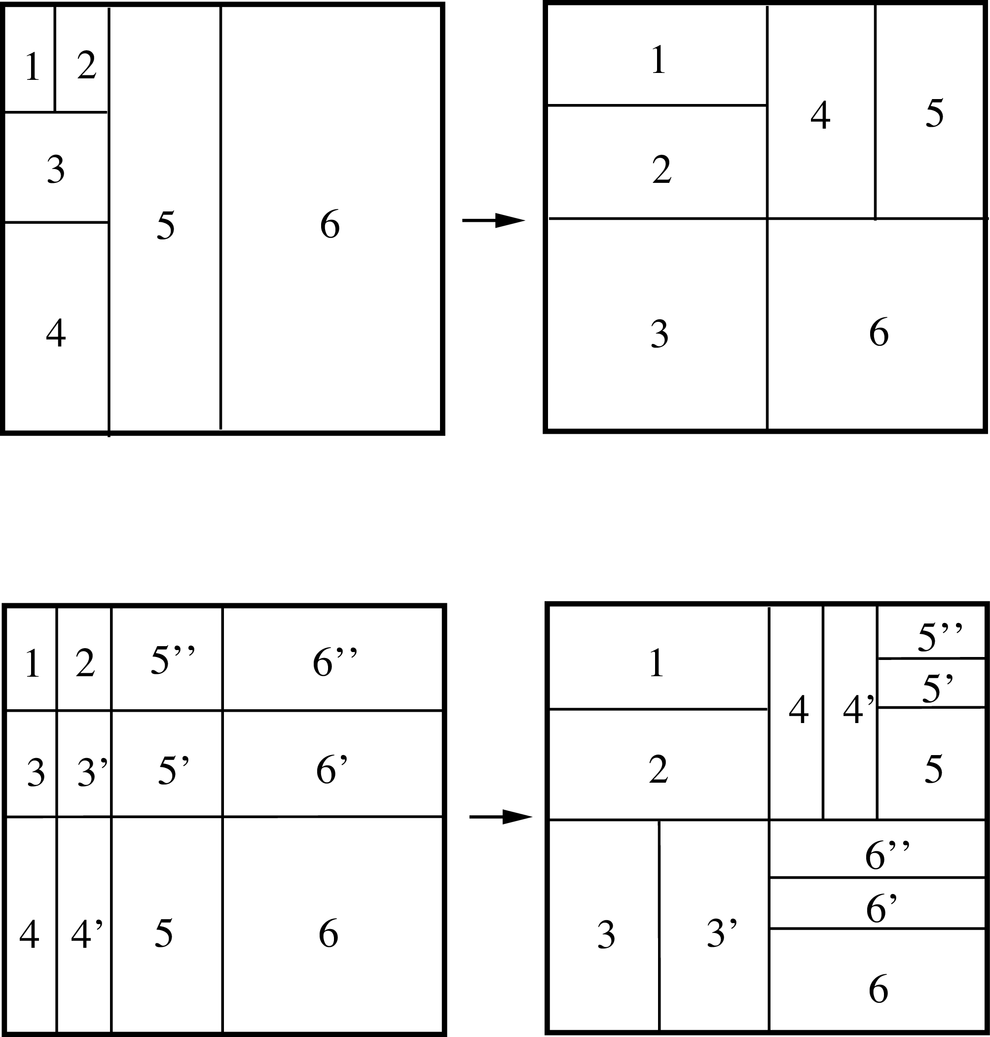
We illustrate in Figure 2 an example of an element w and its resulting grid diagram from the process described above.

Fig. 2.

Two representations of the same element w of 2V. The top representative is not gridded, but is refined to a grid tree-pair diagram in the bottom representation, where the source square is a product of two dyadic subdivisions of the interval.

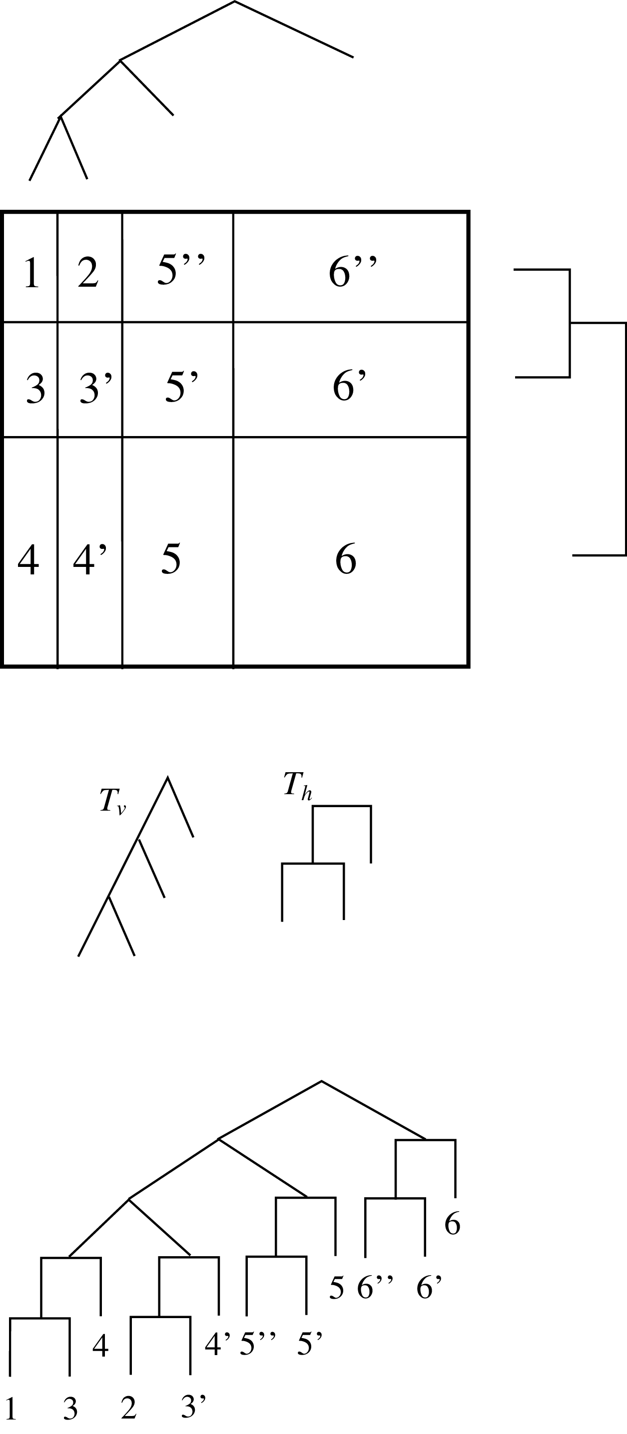
Grid squares can be understood also in terms of trees. Clearly, the grid square can be codified with two trees: one tree representing the dyadic vertical subdivisions and having only triangular, vertical-type, carets, and another tree representing the dyadic horizontal subdivisions, which will have only square, horizontal-type, carets, using the convention described in [ Reference Burillo and Cleary8 ]. We illustrate this process in Figure 3.

Fig. 3.

The source square for the example element w and the two trees that define it. The tree $T_h$ is represented on the right of the square because left leaves represent top halves in subdivisions. At the bottom, a tree representing this subdivision where copies of $T_h$ hang from the leaves of $T_v$ . An analogous tree representative for the same grid subdivision could be constructed with copies of $T_v$ hanging from the leaves of $T_h$ , with the same dyadic blocks occurring, albeit in a different order.

So clearly two trees like these define a unique grid square and vice versa. The actual tree for the square has one copy of the two trees at the root, and many copies of the other tree, each copy hanging from a leaf of the first tree. This can be done in many possible manners. For simplicity, we choose to have the vertical tree at the root and no horizontal trees until the vertical trees are all present, so that the horizontal trees all appear below all of the vertical trees. Other conventionas will give representatives of the same regions, with the left-to-right order of leaves in the two orders will differ, as commonly seen in equivalent tree-based representatives of elements of higher-dimensional Thompson’s groups, but the sets of dyadic blocks will coincide and the potential differing orders may result in a different permutation on the leaves to represent the same group element.

As an example, the standard relation in 2V expressing the simplest interaction between iterated horizontal and vertical subdivisions can be represented with a grid square with one vertical and one horizontal (full-length) subdivision, so both the horizontal and vertical trees used to build the tree will each have a single caret. We assemble these trees in the two possible manners, first hanging two copies of the vertical trees (each a single caret) from each of the two leaves of a single horizontal caret, and then hanging two copies of the horizontal trees (each a single caret) from each of the two leaves of a vertical caret, giving the relation pictured in figure 4 in [ Reference Burillo and Cleary8 ] with a permutation to match the corresponding dyadic blocks.

Fig. 4.

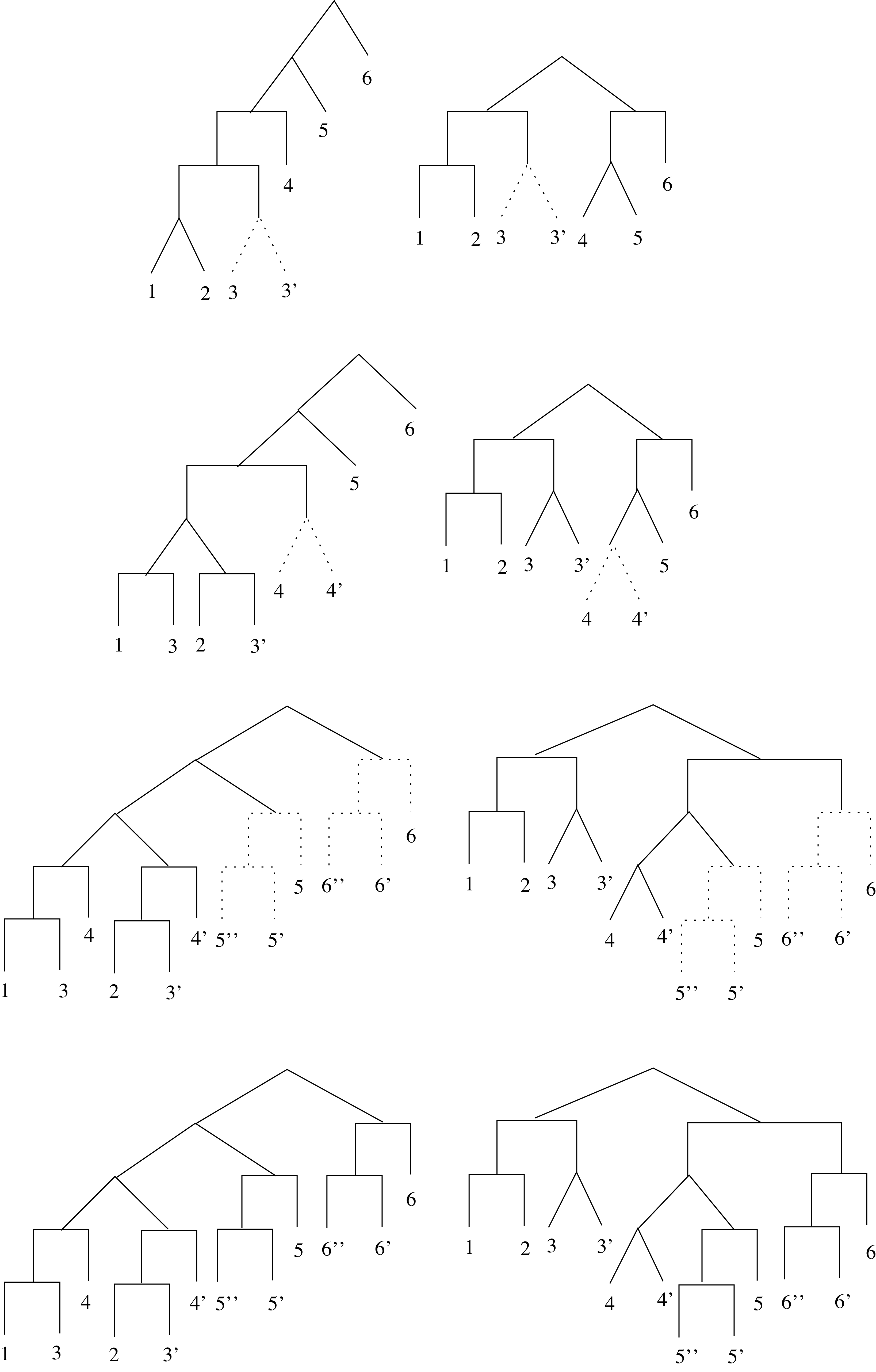
The process of transforming a diagram of our element w into a grid tree-pair diagram. The top tree-pair corresponds to the element w depicted in Figure 2. The process consists of adding vertical-type carets (of triangular type, in dotted lines) needed to apply the defining relation for 2V and bring vertical carets to the top to form the tree $T_v$ . Finally, some horizontal carets (of square type, again dotted) have been added to have full copies of $T_h$ hanging from each leaf of $T_v$ .

The process of taking a subdivided square and finding a grid square for it can also be seen with trees. From a starting tree representative, we can suppose the desire is to have all vertical carets on top and horizontal ones below those. So we may add vertical carets to all leaves that need them so that vertical carets appearing in the tree can be moved up. We illustrate in Figure 4 how this process applies to the example element w from Figures 3 and 4.

3. Reduced grid diagrams

We want to use grid diagrams to extend the notion of reduced diagrams we have in standard Thompson’s groups (such as F, T or V) to 2V. Recall that with relation to standard diagrams such as those in [ Reference Burillo and Cleary8 ], elements of 2V can have more than one reduced tree-pair diagram (reduced in the traditional sense). We will define reduced grid diagrams and prove their uniqueness.

We let f be an element of 2V and we consider a grid diagram for it. The source square is a grid square, so there are two trees $T_v$ and $T_h$ which represent the grid square via the product process described above. The tree $T_v$ has only vertical-type carets and $T_h$ has only horizontal-type carets. We consider the basic dyadic intervals $I_1,I_2,\ldots,I_m$ and $J_1,J_2,\ldots,J_n$ which represent the ordered leaves of the two trees; namely, the $I_i$ are intervals on the bottom edge of the square and the $J_j$ are on the left edge. So each rectangle of the grid is of the type $I_i\times J_j$ , and it naturally is a basic dyadic rectangle.

We observe how there could be a possible reduction of the tree $T_v$ . We would be able to erase a caret of it if its two leaves are represented by intervals $I_i$ and $I_{i+1}$ which could be joined into a single interval. This could only be done if the map f is completely affine in all the rectangles $(I_i\cup I_{i+1})\times J_j$ for every $j=1,2,\ldots,n$ , and the image of each of these basic rectangles is also a basic dyadic rectangle. So we can say that the element is vertically reduced if no caret in $T_v$ can be reduced. That is, for every exposed caret of $T_v$ and its leaves $I_i$ and $I_{i+1}$ , there exists a $j\in\{1,2,\ldots,n\}$ such that the affine map is different on $I_i\times J_j$ and in $I_{i+1}\times J_j$ . Or perhaps it is the same affine map, but the image is not a basic dyadic rectangle.

This notion can be understood easily: a diagram is vertically nonreduced if for an exposed caret in $T_v$ , the whole segment in the square that separates its two leaves could be erased and the map would be the same (and the image of a basic dyadic rectangle is a basic dyadic rectangle), and naturally we say a diagram is vertically reduced if there are no possible vertical reductions.

Clearly we can define an element to be horizontally reduced analogously for the carets on $T_h$ and its rectangles. This leads to the definition of reduced grid tree-pair diagrams.

This just means that the two trees $T_v$ and $T_h$ cannot be reduced, so they are the smallest possible trees which can be used to describe the element via this product subdivision process. If a caret is removed in one of them, then the map f cannot be represented with the grid square corresponding to these two trees.

The main theorem here is the following:

We have developed this construction in 2V for the sake of simplicity, but we observe that grid diagrams generalise readily to nV. A grid cube will have a subdivision into blocks using parts of hyperplanes, and the grid cube can be codified as a product of n trees, each of which has a single type of caret (of the n available types of carets in nV). The process goes the exact same way and the theorems hold with proofs adapted to the n-dimensional case.

4. Metric properties

For the metric properties of nV, we use the word length with respect to one of the finite generating sets. The word length, with respect to any finite generating set, is estimated by Burillo and Cleary [ Reference Burillo and Cleary8 ], in terms of the number of carets, in a minimal-size tree-pair diagram. Such a diagram, although it exists, may be difficult to compute, since finding it could be as difficult as finding a minimal word for the element. Furthermore, such minimal-size tree-pair diagrams are not unique as there may be multiple representatives of a given element, each of minimal size.

Since now we have a unique well-defined diagram for each element, which is easy to compute directly, here we consider the metric properties via the number of carets of the reduced grid diagram, which is unique and algorithmically constructible in an easy way.

So we let x be an element of 2V, and we denote by $|x|$ its word length with respect to the standard finite generating set for 2V of Brin [ Reference Brin4, Reference Brin5 ]. As in [ Reference Burillo and Cleary8 ], we let N(x) be the number of carets in a minimal-size reduced tree diagram for x. And finally, we let M(x) be the number of carets in the reduced grid diagram for x. The result in [ Reference Burillo and Cleary8 ] was that

$$\log N(x) \prec |x| \prec N(x)\log N(x)$$

where $\prec$ means the usual bounds up to multiplicative and additive constants (independent of x) as arise in quasi-isometric embeddings. So we note now that obviously $N(x)\leq M(x)$ (since N is the minimal number of carets), giving M(x) as an obvious upper bound for N(x).

For a lower bound, we note that $M(x)\leq N(x)^2$ by the construction of the grid diagram. To see this, we take the minimal diagram and observe that there are at most N vertical subdivisions and also at most N horizontal ones. So the grid diagram can be constructed with at most $N^2$ rectangles. Then, since $N(x)\leq M(x) \leq N(x)^2$ , $\log N(x)$ and $\log M(x)$ differ at most by a multiplicative constant 2, we have that the lower bound still holds with adjusted linear coefficients. Hence, M(x) satisfies the same inequality as N(x) for estimating word length via the number of carets, giving the following theorem:

Theorem 4·1. The word length $|x|$ of an element $x\in 2V$ , and the number of carets M(x) of its reduced grid diagram satisfy

$$\log M(x) \prec |x| \prec M(x)\log M(x).$$

These bounds cannot be easily improved. The lower bound has the same properties as it did for N(x), since the elements representing the exponential distortion are already represented by grid diagrams (see [ Reference Burillo and Cleary8 ]). For the upper bound, one could speculate that a better quantity to use could be the maximum of the number of carets of $T_h$ and $T_v$ , call this number m(x). But this number would roughly be $m(x)=\sqrt{M(x)}$ , and it would not satisfy an analogous upper bound: the number of elements with a given M is at least $M!$ due to the many possible permutations for those subdivisions, whereas the proposed upper bound $m(x)\log m(x)$ would yield approximately

$$\exp{(m\log m)}=\exp{(\sqrt M \log M)} = M^{\sqrt M}$$

which is smaller than $M!$ . In fact, following arguments parallel to those of Birget [ Reference Birget1 ], we can see that the factorially many possible permutations of the number of blocks in a subdivision means that most of the elements represented by a grid diagram of a fixed size will have word lengths quite close to the upper bound, as was shown by Birget in the case of V.

5. Algebraic normal forms for elements of 2V

5·2. Procedure for subdivision

We suppose that we have a normal form for the grid subdivision of the source square in the manner described in the previous section. For the triangular subdivision tree $T_v$ associated to the vertical gridding, we consider a normal form V associated to the tree that goes from that subdivision to the all-right tree:

$$V=A_0^{a_0}A_1^{a_1}\ldots A_k^{a_k}, $$

where all of the exponents satisfy $a_i\geq 0$ , and $k+1$ is the number of leaves for $T_v$ . For the domain tree, the relevant leaf indices are those from the positive part of the word, and in the case where the gridding occurs entirely in the domain square, we focus on that positive part of the algebraic form, and will write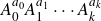 $A_0^{a_0}A_1^{a_1}\cdots A_k^{a_k}$ for that.

Similarly, for the squared caret horizontal subdivision, we have a normal form H for the tree $T_h$ of the type

$$H=B_0^{b_0}B_1^{b_1}\cdots B_{k'}^{b_{k'}}, $$

where again all of the exponents satisfy $b_{i'}\geq 0$ .

One complication is that the generators corresponding non-triangular carets on the spine of the tree are created in a different manner than those on the interior, so that affects the algebraic normal form construction.

We begin by describing what happens to the generators given by the $T_h$ -trees hanging off a leaf of $T_v$ that is not the right-most one. We notice that the word H reappears inserted multiple times in V at each leaf location, with its subindices shifted to account for the increased starting location of the first leaf index. We use H(k) to indicate the word obtained from H by increasing each subindex of the y generators in H by k, and we see a word of the form $A_{i_1} H(...) A_{i_2} H(...) \ldots $ as a positive word in the A- and B-generators for the gridded domain subdivision of the square, where each of the $H(...)$ are the original word for H with appropriate increases in the subindices for the B generators occurring there.

We note that the process of increasing subindices for generators in this manner is a well-known process in F and some of its generalisations that arises in many settings. The shift homomorphism $\phi\;:\; F \rightarrow F$ where $\phi(x_i)=x_{i+1}$ described by Brown and Geoghegan [ Reference Brown and Geoghegan6 ] is an important homotopy idempotent (a universal example, in a sense). Here, the $x_i$ denote the generators in the standard infinite generating set for F. Note that $H(k)= \phi^k(H)$ where $\phi$ is the shift automorphism for the subgroup isomorphic to F created by the generators $B_i$ in the horizontal direction.

What remains is dealing the with the generators given by $T_h$ hanging off of the right-most leaf of $T_v$ . This will involve the generators $B_i$ and $C_j.$ In particular, the smallest index j will correspond to the number of carets on the spine of $T_v.$ The generators $C_j$ will, as in [ Reference Brin3, Reference Burillo and Cleary8 ], appear on the left of the algebraic form. The $B_i$ will correspond to those carets not on the spine of $T_h,$ again shifted upwards depending on the number of leaves in the trees $T_v$ and $T_h$ as above. The word in the $B_j$ will then be behind the last A-generator.

This leads to a positive part P of a normal form, built from the gridded source diagram of the geometric normal form. For the remaining part of the normal form, there is the middle permutational part $\Pi$ given by an appropriate product of conjugates of transpositions of leaves of the all-right tree, followed by a negative word associated to a tree describing the target diagram of the gridded diagram. We note that are there few restrictions on the permutational part or for the negative word as there are many possible elements with the same positive part of the normal form. This gives an algebraic normal form for the element of the type $P\Pi N^{-1}$ .

Fig. 5.

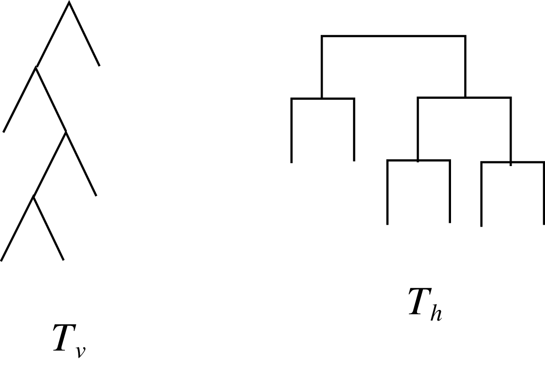
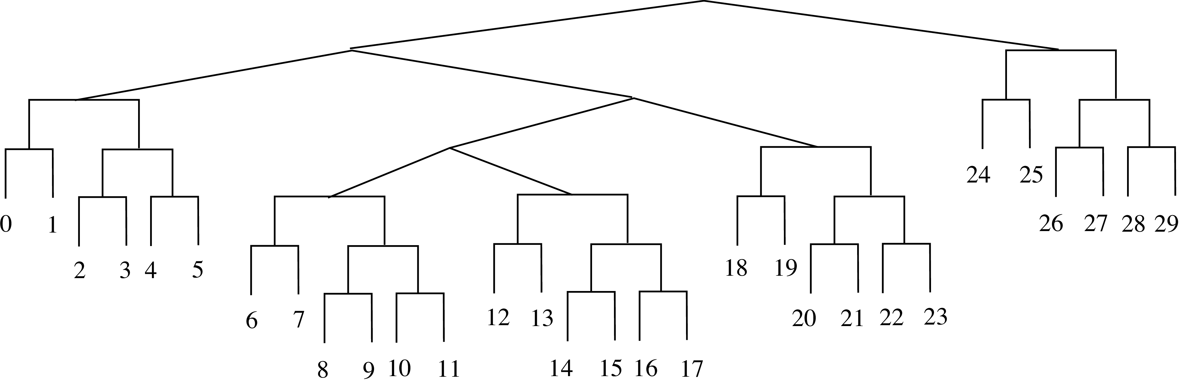
Example trees $T_v$ and and $T_h$ used to construct the positive part of the algebraic normal form for an element v as the vertical and horizontal subdivisions in the product, respectively.

5·3. An illustrative example

Here we illustrate this process via an example element $f \in 2V$ which is sufficiently complicated to show the various cases of the process. We take a grid subdivision whose trees are the vertical and horizontal trees following $T_v$ and $T_h$ respectively, illustrated in Figure 5. As described above, the grid process applies only to the source square, so we neglect in this example the permutational part and the domain subdivision parts of v as either of those could essentially be arbitrary, of the appropriate sizes and subject to not having obvious reductions present.

We construct the corresponding words for the positive part of in the generators. For $T_h$ , this corresponds to the word $A_0A_1^2$ . For convenience, we are going to write this word in the form

$$A_0^{a_0}A_1^{a_1}\cdots A_n^{a_n},$$

where the exponent $a_i$ is allowed to be zero, and so we have all generators listed, each corresponding to a leaf, even if that leaf does not give a positive power for the relevant generator. So our tree $T_v$ corresponds to $A_0A_1^2A_2^0A_3^0A_4^0$ . This will be convenient because this way the generators are in bijection with the leaves of the tree.

We now hang a copy of the tree $T_h$ at each leaf of $T_v$ to obtain the source part of the grid diagram for f. This gives the tree illustrated in Figure 6.

Fig. 6.

The tree used to construct the positive part of the normal form for w, obtained by attaching a copy of $T_h$ below each leaf of $T_v$ .

If a single copy of the tree $T_h$ were alone, the would be represented as a positive element from the leaf exponents method by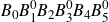 $B_0B_1^0B_2B_3^0B_4B_5^0$ , where again we choose to write zero exponents for the generators not appearing. But when we hang this tree from a leaf (except on the last leaf of $T_v$ ) all carets which are on the spine of the tree now are in the interior, and hence they account for positive powers of generators– even the ones which did not contribute earlier. Some exponents will be increased by 1. So this first instance of the tree $T_h$ hanging from leaf 0 of $T_v$ contributes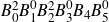 $B_0^2B_1^0B_2^2B_3^0B_4B_5^0$ to the algebraic form.

We inspect the algebraic word that is represented by this large tree of Figure 6. First, there is a power of $A_0$ followed by the word in the B-generators given by $T_h$ :

$$A_0B_0^2B_1^0B_2^2B_3^0B_4B_5^0.$$

The continuation is a power of the next A-generator, which corresponds to $A_1$ but here becomes $A_6$ since $T_h$ has 6 leaves and thus we have the increase in subindex of A. Namely:

$$A_0B_0^2B_1^0B_2^2B_3^0B_4B_5^0\quad A_6^2B_6^2B_7^0B_8^2B_9^0B_{10}B_{11}^0.$$

This process continues with all the words corresponding to all the copies of the tree $T_h$ except the final one. We obtain:

$$\begin{array}cA_0B_0^2B_1^0B_2^2B_3^0B_4B_5^0\quad A_6^2B_6^2B_7^0B_8^2B_9^0B_{10}B_{11}^0\\[4pt] A_{12}^0B_{12}^2B_{13}^0B_{14}^2B_{15}^0B_{16}B_{17}^0\quad A_{18}^0B_{18}^2B_{19}^0B_{20}^2B_{21}^0B_{22}B_{23}^0.\end{array}$$

Finally, since the last copy of $T_h$ is located on the spine of the big tree, it should be modelled on the word on the spine instead of the interior word. Hence it should have some exponents diminished by 1, and also with the corresponding (exponent 0) A at the beginning. The resulting word for the positive part of f is:

$$\begin{array}cA_0B_0^2B_1^0B_2^2B_3^0B_4B_5^0\quad A_6^2B_6^2B_7^0B_8^2B_9^0B_{10}B_{11}^0\quad A_{12}^0B_{12}^2B_{13}^0B_{14}^2B_{15}^0B_{16}B_{17}^0\\[4pt] A_{18}^0B_{18}^2B_{19}^0B_{20}^2B_{21}^0B_{22}B_{23}^0\quad A_{24}^0B_{24}B_{25}^0B_{26}B_{27}^0B_{28}^0B_{29}^0.\end{array}$$

This is not yet the word that corresponds to this tree, because the horizontal carets on the spine (the B-generators that do not occur in the spine version of $T_h$ ) have to be created with C-generators at the beginning of the word. So the exact word that corresponds to this tree is

$$\begin{array}cC_1C_2C_3\quad A_0B_0^2B_1^0B_2^2B_3^0B_4B_5^0\quad A_6^2B_6^2B_7^0B_8^2B_9^0B_{10}B_{11}^0\quad A_{12}^0B_{12}^2B_{13}^0B_{14}^2B_{15}^0B_{16}B_{17}^0\\[4pt] A_{18}^0B_{18}^2B_{19}^0B_{20}^2B_{21}^0B_{22}B_{23}^0\quad A_{24}^0B_{24}B_{25}^0B_{26}B_{27}^0B_{28}^0B_{29}^0.\end{array}$$

Note that this is just the positive part of the normal form, and the representative of the group element will be the positive part described above, followed by generators for the permutational part and then negative powers of the generators describing the tree for the target subdivision.

5·4. General theorem

The procedures of the previous subsections give rise to the following theorem.

Theorem 5·1. Every element $f \in V$ gives rise to a unique prefix word in the letters $A_i, B_j, C_k$ arising from its reduced grid tree-pair diagram as follows: Suppose the source grid gives rise to a vertical tree $T_v$ with $n+1$ leaves and a horizontal tree $T_h$ with $m+1$ leaves. Then:

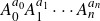
1. (i) $T_v$ corresponds to a word $A_0^{a_0}A_1^{a_1}\cdots A_n^{a_n}$ ; and

2. (ii) $T_h$ corresponds to two words depending upon where in $T_v$ it hangs:

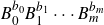
   1. (a) $B_0^{b_0}B_1^{b_1}\cdots B_m^{b_m}$ when it is on the spine ( $b_p$ can be zero);

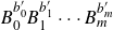
   2. (b) $B_0^{b'_0}B_1^{b'_1}\cdots B_m^{b'_m}$ when it is $\mathbf{not}$ on the spine, (that is, if it hangs from the interior or left side of the tree.) The exponent $b'_p$ is either equal to $b_p$ or $b_{p}+1$ depending on the generator.

Furthermore, the full tree corresponding to the source grid admits a unique word made out of the concatenation of the following words:

1. (iii) a word of the type $C_iC_{i+1}\ldots C_{i+\ell}$ corresponding to the horizontal carets on the spine of $T_h$ , where the indices are all consecutive to create the right-hand side carets of the appropriate types;

2. (iv) n words of the type

   $$A_{(m+1)j}^{a_j}B_{(m+1)j}^{b'_0}B_{(m+1)j+1}^{b'_1}\ldots B_{(m+1)j+m}^{b'_m}$$
   for $j=0,1,\ldots,n-1$ ;

3. (v) a final word, of the type

   $$A_{(m+1)n}^{a_n}B_{(m+1)n}^{b_0}B_{(m+1)n+1}^{b_1}\ldots B_{(m+1)n+m}^{b_m}.$$

Proof. This follows from [ Reference Burillo and Cleary8 , theorem 2·2], Theorem 3·2, and the setup and process described in Subsections 5·1 and 5·2 and illustrated in Subsection 5·3.

In the example above, we have $i=1$ , $\ell=2$ , $n=4$ , and $m=5$ . The introduction of the generators with exponent zero helps understand its regularity, but it makes the word unnecessarily long. If we eliminate the terms with exponent 0, the word for the positive part of v becomes just

$$C_1C_2C_3\quad A_0B_0^2B_2^2B_4\quad A_6^2B_6^2B_8^2B_{10}\quad B_{12}^2B_{14}^2B_{16}\quad B_{18}^2B_{20}^2B_{22}\quad B_{24}B_{26}$$

which can be checked by reading exponents and generators directly from the tree.

Recall that these algebraic forms are with respect to the standard infinite generating sets $\{A_i, B_i, C_i, \Pi_i, \overline{\Pi_i}\}$ described by Brin [ Reference Brin3 ]. Using the standard expressions of the infinite generators in terms of the finite generating set $\Sigma$ described by Brin [ Reference Brin3 ] as $\{A_0, A_1, B_0, B_1, \Pi_0, \overline{\Pi_0}, \Pi_1, \overline{\Pi_1}\}$ via substitution, the standard expressions with respect to the infinite generating set give rise to standard expressions of elements with respect to the finite generating sets of the type $\Sigma$ . So grid tree diagrams give standard algebraic normal forms both with respect to infinite and finite generating sets.

6. Other grid normal forms and higher dimensional cases

In the higher dimensional cases of nV, there are similar grid diagrams arising from the partitions of the n-dimensional cube along each of its coordinates. For the tree representative, we use n different types of carets (possibly triangular, square, rounded, …) and again can obtain a grid subdivision which can be regarded as a product subdivision of the appropriate dimensional unit cube via n dyadic subdivisions of each of the n coordinates. There are natural generalisations of Proposition 2·3 and Theorem 3·2 giving that such elements have grid diagrams and that they are unique. The metric estimates of Theorem 4·1 also hold in nV as instead of the number of carets growing quadratically at most, the number of carets in the gridding process grows at most as the nth power, but that potential growth still may be absorbed by adjusting the multiplicative constants outside of the logarithms in the metric bound estimates. The algebraic form of Theorem 5·1 also give canonical normal forms, albeit more complicated as the natural “nesting” of the copies of the trees will lead to many terms. For the positive part of the word, there will be the same components. There will be a prefix word of generators of $n-1$ types to create the correct shape of the spine of the tree, followed by a word in a standard form obtained by a nesting process. Starting with words in the A generators, each gap between the powers of the A generators will interrupted by subwords for the B generators (with shifted indices, as above), and for which those B subwords themselves will be interrupted by shifted index subwords of generators for each additional dimension in a natural recursive manner, nesting to give a standard normal form for the positive part of the word.

Also, we note that in 2V, there was a choice to grid both of the coordinates in the source cube. There are other possible choices, each of which would lead to standard forms for that choice. For example, we could have chosen to grid the target cube, or to grid the horizontal component in the source together with the vertical component in the target. We can regard that decision as assigning to each coordinate a binary choice of that coordinate lying in either the source or target. So there are 4 such possible choices for 2V and $2^n$ potential choices for nV, with each of those choices giving grid normal forms and associated algebraic normal forms. Typically we presume that the normal forms are most useful when either the source or the target cube is completely gridded, rather than sharing the gridding between the two cubes, but there are many possible choices, each leading to a unique form for every element. If we consider subdivisions where the coordinates lie in $\mathbf{Z}[1/p]$ for the corresponding versions of nV, these methods give completely analogous results using multiple types of carets with p children in the place of the multiple types of binary carets used above. Similarly, for the groups nBV where the matchings between the subdivisions are given as braids in the appropriate dimensional spaces rather than permutations, there are similar standard forms for the positive and negative parts of the word, with a middle word in a standard form chosen for the appropriate braid representation.