





1. Introduction
The study of individual movement has attracted significant attention in the theoretical exploration of mathematical biology [Reference Cantrell and Cosner6, Reference Lou19, Reference Okubo and Levin23]. Reaction-diffusion models are widely used to describe spatial heterogeneity and individual movement. However, the dispersal rate is one of the hardest parameters to estimate despite its importance, leading to a limited understanding of diffusion processes in many cases.
In [Reference Allen, Bolker, Lou and Nevai1], Allen et al. proposed a frequency-dependent susceptible-infected-susceptible (SIS) reaction-diffusion model for a population inhabiting a continuous spatial habitat, where the Brownian motion is applied to describe the diffusion of individuals with constant diffusion rates, which is in the form of
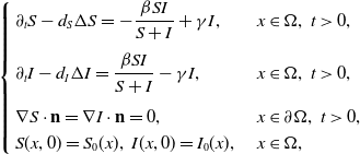 \begin{equation} \left \{\begin{aligned} &\partial _t S-d_S\Delta S=-\frac {\beta SI}{S+I}+\gamma I,\ & x&\in \Omega ,\ t\gt 0,\\[4pt] &\partial _t I-d_I\Delta I=\frac {\beta SI}{S+I}-\gamma I,\ & x&\in \Omega ,\ t\gt 0,\\[4pt] &\displaystyle \nabla S\cdot \mathbf{n}=\nabla I\cdot \mathbf{n}=0,\ & x&\in \partial \Omega ,\ t\gt 0,\\ &S(x,0)=S_0(x),\ I(x,0)=I_0(x),\ & x&\in \Omega , \end{aligned}\right . \end{equation}
where $\Omega \subset \mathbb{R}^n(n\geq 1)$
is a bounded domain with smooth boundary
$\Omega \subset \mathbb{R}^n(n\geq 1)$
is a bounded domain with smooth boundary $\partial \Omega$
, and
$\partial \Omega$
, and $\mathbf{n}$
is the unit outward normal vector on the boundary.
$\mathbf{n}$
is the unit outward normal vector on the boundary. $S\,:\!=\,S(x,t)$
and
$S\,:\!=\,S(x,t)$
and $I\,:\!=\,I(x,t)$
denote the densities of susceptible and infected individuals at location
$I\,:\!=\,I(x,t)$
denote the densities of susceptible and infected individuals at location $x$
and time
$x$
and time $t$
, respectively.
$t$
, respectively. $\beta \,:\!=\,\beta (x)$
and
$\beta \,:\!=\,\beta (x)$
and $\gamma \,:\!=\,\gamma (x)$
, which measure the infection rate and recovery rate, respectively, are positive H
$\gamma \,:\!=\,\gamma (x)$
, which measure the infection rate and recovery rate, respectively, are positive H $\ddot {\mathrm{o}}$
lder continuous functions on
$\ddot {\mathrm{o}}$
lder continuous functions on $\Omega$
. Homogeneous Neumann boundary conditions are selected to signify the zero population flux across the boundary. The frequency-dependent incidence
$\Omega$
. Homogeneous Neumann boundary conditions are selected to signify the zero population flux across the boundary. The frequency-dependent incidence $\frac {\beta SI}{S+I}$
, also known as standard incidence, is a Lipschitz continuous function of
$\frac {\beta SI}{S+I}$
, also known as standard incidence, is a Lipschitz continuous function of $S$
and
$S$
and $I$
in the open first quadrant, and its definition can be extended to the entire first quadrant by assigning it a value of zero when either
$I$
in the open first quadrant, and its definition can be extended to the entire first quadrant by assigning it a value of zero when either $S=0$
or
$S=0$
or $I=0$
. Model (1.1) is a weakly coupled semilinear parabolic system, where ‘weakly coupled’ means that the
$I=0$
. Model (1.1) is a weakly coupled semilinear parabolic system, where ‘weakly coupled’ means that the $S$
-equation contains no derivatives of
$S$
-equation contains no derivatives of $I$
, and the
$I$
, and the $I$
-equation contains no derivatives of
$I$
-equation contains no derivatives of $S$
. Given that the sign of
$S$
. Given that the sign of $\beta -\gamma$
varies across the domain
$\beta -\gamma$
varies across the domain $\Omega$
, the basic reproduction number
$\Omega$
, the basic reproduction number $\mathcal{R}_0$
(1.1) is defined by variational characterization:
$\mathcal{R}_0$
(1.1) is defined by variational characterization:
 \begin{equation} \mathcal{R}_0^{(1.1)}=\sup _{0\neq \varphi \in H^1(\Omega )}\left \{\frac {\int _\Omega \beta \varphi ^2dx}{\int _\Omega (d_I|\nabla \varphi |^2+\gamma \varphi ^2)dx}\right \}\!. \end{equation}
It is verified in [Reference Allen, Bolker, Lou and Nevai1] that $\mathcal{R}_0$
(1.1) is a monotone decreasing function of
$\mathcal{R}_0$
(1.1) is a monotone decreasing function of $d_I$
with
$d_I$
with $\mathcal{R}_0$
(1.1)
$\mathcal{R}_0$
(1.1) $\rightarrow \max _{x\in \bar {\Omega }}\{\beta /\gamma \}$
as
$\rightarrow \max _{x\in \bar {\Omega }}\{\beta /\gamma \}$
as $d_I\rightarrow 0$
and
$d_I\rightarrow 0$
and $\mathcal{R}_0$
(1.1)
$\mathcal{R}_0$
(1.1) $\rightarrow \int _\Omega \beta dx/\int _\Omega \gamma dx$
as
$\rightarrow \int _\Omega \beta dx/\int _\Omega \gamma dx$
as $d_I\rightarrow \infty$
.
$d_I\rightarrow \infty$
.
It can be observed that individual movement in (1.1) is random and irregular. Recently, Wang et al. introduced two forms of cognitive diffusion in terms of two types of law of diffusion to depict population movement with infection concerns most straightforwardly [Reference Wang, Wang and Kim29]. The dispersal functions adopted in [Reference Wang, Wang and Kim29] were taken in the following sense. Susceptible individuals will leave the position with a high infection rate $\beta$
rapidly to avoid being infected, while infected individuals will remain in the position with a high recovery rate
$\beta$
rapidly to avoid being infected, while infected individuals will remain in the position with a high recovery rate $\gamma$
to access more medical treatment. Therefore, the diffusion rate of susceptibles is high in positions with a high infection rate, while the diffusion rate of infectives is low in positions with a high recovery rate. From the perspective of patch models, one of the cognitive diffusions is called symmetric diffusion, which follows Fickian law of diffusion [Reference Fick13]. Replacing the non-directional diffusion in (1.1) by the symmetric diffusion leads to
$\gamma$
to access more medical treatment. Therefore, the diffusion rate of susceptibles is high in positions with a high infection rate, while the diffusion rate of infectives is low in positions with a high recovery rate. From the perspective of patch models, one of the cognitive diffusions is called symmetric diffusion, which follows Fickian law of diffusion [Reference Fick13]. Replacing the non-directional diffusion in (1.1) by the symmetric diffusion leads to
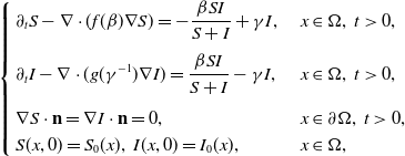 \begin{equation} \left \{\begin{aligned} &\partial _t S-\nabla \cdot (f(\beta )\nabla S)=-\frac {\beta SI}{S+I}+\gamma I,\ & x&\in \Omega ,\ t\gt 0,\\[4pt] &\partial _t I-\nabla \cdot (g(\gamma ^{-1})\nabla I)=\frac {\beta SI}{S+I}-\gamma I,\ & x&\in \Omega ,\ t\gt 0,\\[4pt] &\displaystyle \nabla S\cdot \mathbf{n}=\nabla I\cdot \mathbf{n}=0,\ & x&\in \partial \Omega ,\ t\gt 0,\\ &S(x,0)=S_0(x),\ I(x,0)=I_0(x),\ & x&\in \Omega , \end{aligned}\right . \end{equation}
where $f(\beta )$
and
$f(\beta )$
and $g(\gamma ^{-1})$
are dispersal functions of susceptible and infected individuals, respectively.
$g(\gamma ^{-1})$
are dispersal functions of susceptible and infected individuals, respectively. $f$
and
$f$
and $g$
are increasing functions of
$g$
are increasing functions of $\beta$
and
$\beta$
and $\gamma ^{-1}$
, respectively. The other one is random diffusion, which follows the Fokker–Planck-type law (also known as Chapman’s law) of diffusion [Reference Chapman7]. The corresponding system equipped with random diffusion becomes
$\gamma ^{-1}$
, respectively. The other one is random diffusion, which follows the Fokker–Planck-type law (also known as Chapman’s law) of diffusion [Reference Chapman7]. The corresponding system equipped with random diffusion becomes
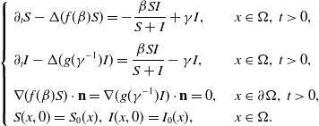 \begin{equation} \left \{\begin{aligned} &\partial _t S-\Delta (f(\beta )S)=-\frac {\beta SI}{S+I}+\gamma I,\ & x&\in \Omega ,\ t\gt 0,\\[4pt] &\partial _t I-\Delta (g(\gamma ^{-1})I)=\frac {\beta SI}{S+I}-\gamma I,\ & x&\in \Omega ,\ t\gt 0,\\[4pt] &\displaystyle \nabla (f(\beta )S)\cdot \mathbf{n}=\nabla (g(\gamma ^{-1})I)\cdot \mathbf{n}=0,\ & x&\in \partial \Omega ,\ t\gt 0,\\ &S(x,0)=S_0(x),\ I(x,0)=I_0(x),\ & x&\in \Omega . \end{aligned}\right . \end{equation}
The diffusion rates in models (1.3) and (1.4) are functions depending only on infection and recovery rates. We can find that the epidemic models (1.3) and (1.4) with cognitive diffusion remain weakly coupled semilinear parabolic systems. Obviously, if the dispersal rates $f(\beta )$
and
$f(\beta )$
and $g(\gamma ^{-1})$
are spatially homogeneous, i.e.,
$g(\gamma ^{-1})$
are spatially homogeneous, i.e., $f(\beta (x))=f(\beta (y))$
and
$f(\beta (x))=f(\beta (y))$
and $g((\gamma (x))^{-1})=g((\gamma (y))^{-1})$
for any
$g((\gamma (x))^{-1})=g((\gamma (y))^{-1})$
for any $x,y\in \Omega$
, then the dispersal rates become two constants. Accordingly, the random and symmetric diffusion reduces to the homogeneous diffusion in (1.1). The basic reproduction number for (1.3) is defined as
$x,y\in \Omega$
, then the dispersal rates become two constants. Accordingly, the random and symmetric diffusion reduces to the homogeneous diffusion in (1.1). The basic reproduction number for (1.3) is defined as
 \begin{equation*} \mathcal{R}_0^{(1.3)}=\sup _{0\neq \varphi \in H^1(\Omega )}\left \{\frac {\int _\Omega \beta \varphi ^2dx}{\int _\Omega (g(\gamma ^{-1})|\nabla \varphi |^2+\gamma \varphi ^2)dx}\right \}\!. \end{equation*}
If it is further assumed that $g(\gamma ^{-1})=\eta g_1(\gamma ^{-1})$
, where
$g(\gamma ^{-1})=\eta g_1(\gamma ^{-1})$
, where $\eta$
is a positive constant and
$\eta$
is a positive constant and $g_1\gt 0$
is a smooth function. It is observed that
$g_1\gt 0$
is a smooth function. It is observed that $\mathcal{R}_0$
(1.3) exhibits similar asymptotic properties concerning
$\mathcal{R}_0$
(1.3) exhibits similar asymptotic properties concerning $\eta$
for a fixed
$\eta$
for a fixed $g_1$
as
$g_1$
as $\mathcal{R}_0$
(1.1) does with respect to
$\mathcal{R}_0$
(1.1) does with respect to $d_I$
. The basic reproduction number for (1.4) can be characterized as
$d_I$
. The basic reproduction number for (1.4) can be characterized as
 \begin{equation*} \mathcal{R}_0^{(1.4)}=\sup _{0\neq \varphi \in H^1(\Omega )}\left \{\frac {\int _\Omega \beta /g_1(\gamma ^{-1})\varphi ^2dx}{\int _\Omega (\eta |\nabla \varphi |^2+\gamma /g_1(\gamma ^{-1}) \varphi ^2)dx}\right \}\!. \end{equation*}
Similarly, the basic reproduction number $\mathcal{R}_0$
(1.4)
$\mathcal{R}_0$
(1.4) $\rightarrow \max _{x\in \bar {\Omega }}\{\beta /\gamma \}$
as
$\rightarrow \max _{x\in \bar {\Omega }}\{\beta /\gamma \}$
as $\eta \rightarrow 0$
and
$\eta \rightarrow 0$
and $\mathcal{R}_0$
(1.4)
$\mathcal{R}_0$
(1.4) $\rightarrow \int _\Omega \beta g_1(\gamma ^{-1})dx/\int _\Omega \gamma g_1(\gamma ^{-1})dx$
as
$\rightarrow \int _\Omega \beta g_1(\gamma ^{-1})dx/\int _\Omega \gamma g_1(\gamma ^{-1})dx$
as $\eta \rightarrow \infty$
.
$\eta \rightarrow \infty$
.
According to news or reports on infectious diseases, susceptibles move rapidly at positions with a high number of new infections. It is more reasonable to depict the diffusion rate of susceptible individuals through new infection cases since the infection rate is hard to perceive. The diffusion rate of infected individuals is still assumed to depend on the recovery rate. We continue to adopt Fickian and the Fokker–Planck-type laws of diffusion as in [Reference Wang, Wang and Kim29] to illustrate individual movement. The corresponding systems become
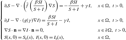 \begin{equation} \left \{\begin{aligned} &\partial _t S-\nabla \cdot \left (\tilde {f}\left (\frac {\beta SI}{S+I}\right )\nabla S\right )=-\frac {\beta SI}{S+I}+\gamma I,\ & x&\in \Omega ,\ t\gt 0,\\[3pt] &\partial _t I-\nabla \cdot (g(\gamma )\nabla I)=\frac {\beta SI}{S+I}-\gamma I,\ & x&\in \Omega ,\ t\gt 0,\\ & \nabla S\cdot \mathbf{n}=\nabla I\cdot \mathbf{n}=0,\ & x&\in \partial \Omega ,\ t\gt 0,\\ &S(x,0)=S_0(x),\ I(x,0)=I_0(x),\ & x&\in \Omega , \end{aligned}\right . \end{equation}
and
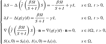 \begin{equation} \left \{\begin{aligned} &\partial _t S-\Delta \left (\tilde {f}\left (\frac {\beta SI}{S+I}\right )S\right )=-\frac {\beta SI}{S+I}+\gamma I,\ & x&\in \Omega ,\ t\gt 0,\\[3pt] &\partial _t I-\Delta (g(\gamma )I)=\frac {\beta SI}{S+I}-\gamma I,\ & x&\in \Omega ,\ t\gt 0,\\[3pt] & \nabla \left (\tilde {f}\left (\frac {\beta SI}{S+I}\right )S\right )\cdot \mathbf{n}=\nabla (g(\gamma )I)\cdot \mathbf{n}=0,\ & x&\in \partial \Omega ,\ t\gt 0,\\[3pt] &S(x,0)=S_0(x),\ I(x,0)=I_0(x),\ & x&\in \Omega , \end{aligned}\right . \end{equation}
respectively. Here, $\tilde {f}$
is an increasing function of
$\tilde {f}$
is an increasing function of $\frac {\beta SI}{S+I}$
, and
$\frac {\beta SI}{S+I}$
, and $g$
is a decreasing function of
$g$
is a decreasing function of $\gamma$
. Models (1.5) and (1.6) transform the semilinear parabolic systems (1.3) and (1.4) into strongly coupled quasilinear parabolic systems, where ‘strongly coupled’ means that the derivative of
$\gamma$
. Models (1.5) and (1.6) transform the semilinear parabolic systems (1.3) and (1.4) into strongly coupled quasilinear parabolic systems, where ‘strongly coupled’ means that the derivative of $I$
appears in the
$I$
appears in the $S$
-equation.
$S$
-equation.
From the perspective of population interactions driving spatial movement, model (1.6) can be interpreted as a cross-diffusion model. Let $f(\beta ,S,I)(x)\,:\!=\,\tilde {f}\big (\frac {\beta SI}{S+I}\big )$
for all
$f(\beta ,S,I)(x)\,:\!=\,\tilde {f}\big (\frac {\beta SI}{S+I}\big )$
for all $x\in \bar {\Omega }$
. We use
$x\in \bar {\Omega }$
. We use $f_\beta$
,
$f_\beta$
, $f_S$
and
$f_S$
and $f_I$
to denote the partial derivatives of
$f_I$
to denote the partial derivatives of $f$
with respect to
$f$
with respect to $\beta$
,
$\beta$
, $S$
and
$S$
and $I$
, respectively.
$I$
, respectively. $g^{\prime}$
means the derivative of
$g^{\prime}$
means the derivative of $g$
with respect to
$g$
with respect to $\gamma$
. By expanding the Laplace operator, the Fokker–Planck-type diffusion term in the first equation of (1.6) can be written as
$\gamma$
. By expanding the Laplace operator, the Fokker–Planck-type diffusion term in the first equation of (1.6) can be written as
 \begin{eqnarray*} \Delta (f(\beta ,S,I)S)&=&\nabla \cdot (f(\beta ,S,I)\nabla S)+\nabla \cdot (S\nabla f(\beta ,S,I) )\\ &=&\nabla \cdot (f_\beta S\nabla \beta )+\nabla \cdot ((f(\beta ,S,I)+f_S S)\nabla S+f_I S\nabla I). \end{eqnarray*}
It consists of self- and cross-diffusive flux, where $f(\beta ,S,I)+f_S S$
signifies the self-diffusion pressure and
$f(\beta ,S,I)+f_S S$
signifies the self-diffusion pressure and $f_I S$
measures the cross-diffusion pressure acting on the population
$f_I S$
measures the cross-diffusion pressure acting on the population $S$
by
$S$
by $I$
. The advection and growth adaptation [Reference Bengfort, Malchow and Hilker5] of susceptible individuals are included in the term
$I$
. The advection and growth adaptation [Reference Bengfort, Malchow and Hilker5] of susceptible individuals are included in the term $\nabla \cdot (f_\beta S\nabla \beta )$
. The Fokker–Planck-type diffusion term in the second equation of (1.6) can be written as
$\nabla \cdot (f_\beta S\nabla \beta )$
. The Fokker–Planck-type diffusion term in the second equation of (1.6) can be written as
 \begin{eqnarray*} \Delta (g(\gamma )I)=\nabla \cdot (g^{\prime} I\nabla \gamma +g(\gamma )\nabla I), \end{eqnarray*}
where $g(\gamma )$
is the self-diffusion pressure, and
$g(\gamma )$
is the self-diffusion pressure, and $\nabla \cdot (g^{\prime} I\nabla \gamma )$
includes the advection and growth adaptation of infected individuals. However, model (1.5) only includes self-diffusion terms. From the perspective of a matrix, the diffusion terms in (1.5) are of the diagonal form, while in (1.6) are of upper-triangular form since the cross-diffusion term occurs only in the first equation. In [Reference Shigesada, Kawasaki and Teramoto25], Shigesada et al. proposed a cross-diffusion model to analyse the distributional pattern formation of two species in heterogeneous environments. Lou and Ni studied self-diffusion and cross-diffusion by considering the corresponding elliptic system in [Reference Lou and Ni20]. In addition to this, a series of works [Reference Choi, Lui and Yamada8, Reference Choi, Lui and Yamada9, Reference Le15, Reference Le, Nguyen and Nguyen16, Reference Lou, Ni and Wu21, Reference Tuoc28] investigated the existence of the solution of the cross-diffusion model under different conditions. Different from the models investigated in the above works, the diffusion pressure in models (1.5) and (1.6) is spatially variant.
$\nabla \cdot (g^{\prime} I\nabla \gamma )$
includes the advection and growth adaptation of infected individuals. However, model (1.5) only includes self-diffusion terms. From the perspective of a matrix, the diffusion terms in (1.5) are of the diagonal form, while in (1.6) are of upper-triangular form since the cross-diffusion term occurs only in the first equation. In [Reference Shigesada, Kawasaki and Teramoto25], Shigesada et al. proposed a cross-diffusion model to analyse the distributional pattern formation of two species in heterogeneous environments. Lou and Ni studied self-diffusion and cross-diffusion by considering the corresponding elliptic system in [Reference Lou and Ni20]. In addition to this, a series of works [Reference Choi, Lui and Yamada8, Reference Choi, Lui and Yamada9, Reference Le15, Reference Le, Nguyen and Nguyen16, Reference Lou, Ni and Wu21, Reference Tuoc28] investigated the existence of the solution of the cross-diffusion model under different conditions. Different from the models investigated in the above works, the diffusion pressure in models (1.5) and (1.6) is spatially variant.
Considering the epidemic dynamics becomes intriguing if the diffusion rate of infected individuals depends on new recovery cases $\gamma I$
. We write the diffusion rate of infective individuals as
$\gamma I$
. We write the diffusion rate of infective individuals as $g(\gamma ,I)(x)\,:\!=\,\tilde {g}(\gamma I)$
, where
$g(\gamma ,I)(x)\,:\!=\,\tilde {g}(\gamma I)$
, where $\tilde {g}$
is a decreasing function of
$\tilde {g}$
is a decreasing function of $\gamma I$
. The Fokker–Planck-type diffusion term in the
$\gamma I$
. The Fokker–Planck-type diffusion term in the $I$
-equation can be written as
$I$
-equation can be written as
 \begin{equation*}\Delta (g(\gamma ,I)I)=\nabla \cdot [(g(\gamma ,I)+g_I I)\nabla I+g_\gamma I\nabla \gamma ],\end{equation*}
where $g_\gamma$
and
$g_\gamma$
and $g_I$
represent the partial derivatives of
$g_I$
represent the partial derivatives of $g$
with respect to
$g$
with respect to $\gamma$
and
$\gamma$
and $I$
, respectively. The
$I$
, respectively. The $I$
-equations with boundary conditions in models (1.5) and (1.6) are then replaced by
$I$
-equations with boundary conditions in models (1.5) and (1.6) are then replaced by
 \begin{equation} \left \{\begin{aligned} &\partial _t I-\nabla \cdot (g(\gamma , I)\nabla I)=\frac {\beta SI}{S+I}-\gamma I,\ & x&\in \Omega ,\ t\gt 0,\\ &\nabla I\cdot \mathbf{n}=0,\ & x&\in \partial \Omega ,\ t\gt 0, \end{aligned}\right . \end{equation}
and
 \begin{equation} \left \{\begin{aligned} &\partial _t I-\Delta (g(\gamma , I)I)=\frac {\beta SI}{S+I}-\gamma I,\ & x&\in \Omega ,\ t\gt 0,\\ &\nabla (g(\gamma , I)I)\cdot \mathbf{n}=0,\ & x&\in \partial \Omega ,\ t\gt 0, \end{aligned}\right . \end{equation}
respectively.
We assume that the initial total number of individuals for both models (1.5) and (1.6) is $N$
. By use of the zero-flux boundary conditions, adding the first two equations of (1.5) and integrating the result over
$N$
. By use of the zero-flux boundary conditions, adding the first two equations of (1.5) and integrating the result over $\Omega$
by parts lead to
$\Omega$
by parts lead to
 \begin{equation} \int _\Omega (S+I)dx=\int _\Omega (S_0+I_0)dx=N. \end{equation}
This implies that the total population is constant. By the divergence theorem, this conservation law extends to model (1.6), implying that the total number of individuals is invariant and that (1.9) remains valid. We take three types of dependence of diffusion rates on new infection or recovery cases, or the recovery rate:
-
• Linear dependence: $f(\beta ,S,I)=k\frac {\beta SI}{S+I}+\eta$
,
$g(\gamma ,I)=k(\gamma I)^{-1}+\eta$
,
$g(\gamma )=k\gamma ^{-1}+\eta$
;
$f(\beta ,S,I)=k\frac {\beta SI}{S+I}+\eta$
,
$g(\gamma ,I)=k(\gamma I)^{-1}+\eta$
,
$g(\gamma )=k\gamma ^{-1}+\eta$
; -
• Exponential dependence:
$f(\beta ,S,I)=\displaystyle \eta e^{ \frac {k\beta SI}{S+I}}$
,
$g(\gamma ,I)=\eta e^{-k\gamma I}$
,
$g(\gamma )=\eta e^{-k\gamma }$
; -
• Algebraic dependence:
$f(\beta ,S,I)=\eta \left (1+\frac {\beta SI}{S+I}\right )^k$
,
$g(\gamma ,I)=\eta (1+\gamma I)^{-k}$
,
$g(\gamma )=\eta (1+\gamma )^{-k}$
.









Here, $k$
and
$k$
and $\eta$
are positive constants. The exponentially and algebraically dependent functions were explored in [Reference Tang and Wang27, Reference Wang and Xu30]. We impose the following assumptions on systems (1.5) and (1.6):
$\eta$
are positive constants. The exponentially and algebraically dependent functions were explored in [Reference Tang and Wang27, Reference Wang and Xu30]. We impose the following assumptions on systems (1.5) and (1.6):
(H1) $\beta$
and
$\beta$
and $\gamma$
are positive
$\gamma$
are positive $C^1$
functions for all
$C^1$
functions for all $x\in \bar {\Omega }$
. Furthermore,
$x\in \bar {\Omega }$
. Furthermore, $\beta ^*\,:\!=\,\max _{x\in \bar {\Omega }} \beta$
,
$\beta ^*\,:\!=\,\max _{x\in \bar {\Omega }} \beta$
, $\beta _*\,:\!=\,\min _{x\in \bar {\Omega }} \beta$
,
$\beta _*\,:\!=\,\min _{x\in \bar {\Omega }} \beta$
, $\gamma ^*\,:\!=\,\max _{x\in \bar {\Omega }} \gamma$
and
$\gamma ^*\,:\!=\,\max _{x\in \bar {\Omega }} \gamma$
and $\gamma _*\,:\!=\,\min _{x\in \bar {\Omega }} \gamma$
.
$\gamma _*\,:\!=\,\min _{x\in \bar {\Omega }} \gamma$
.
(H2) $\eta \leq f(\beta ,S,I)\in C^2([\beta _*,\beta ^*]\times [0,+\infty )^2)$
and
$\eta \leq f(\beta ,S,I)\in C^2([\beta _*,\beta ^*]\times [0,+\infty )^2)$
and $0\leq f_\beta (\beta ,S,I),f_S(\beta ,S,I),f_I(\beta ,S,I)$
on
$0\leq f_\beta (\beta ,S,I),f_S(\beta ,S,I),f_I(\beta ,S,I)$
on $[\beta _*,\beta ^*]\times [0,+\infty )^2$
.
$[\beta _*,\beta ^*]\times [0,+\infty )^2$
.
(H3) $0\lt g(\gamma )\in C^2([\gamma _*,\gamma ^*])$
and
$0\lt g(\gamma )\in C^2([\gamma _*,\gamma ^*])$
and $g^{\prime}(\gamma )\leq 0$
.
$g^{\prime}(\gamma )\leq 0$
.
(H4) $S_0(x), I_0(x)\geq 0$
for all
$S_0(x), I_0(x)\geq 0$
for all $x\in \bar {\Omega }$
and
$x\in \bar {\Omega }$
and $\int _\Omega I_0(x)dx\gt 0$
.
$\int _\Omega I_0(x)dx\gt 0$
.
Assumptions (H2) and (H3) are reasonable when we choose $f$
and
$f$
and $g$
in the three forms as above. Individual movement persists regardless of the presence of an infectious disease. We assume the constant diffusion rate is
$g$
in the three forms as above. Individual movement persists regardless of the presence of an infectious disease. We assume the constant diffusion rate is $\eta$
when we take the above three forms of dispersal functions with
$\eta$
when we take the above three forms of dispersal functions with $I=0$
. When considering the nonnegative steady-state solutions
$I=0$
. When considering the nonnegative steady-state solutions $(S(x),I(x))$
of (1.5) and (1.6), we regard the solution with
$(S(x),I(x))$
of (1.5) and (1.6), we regard the solution with $I(x)=0$
for all
$I(x)=0$
for all $x\in \Omega$
as a disease-free equilibrium (DFE) and the solution with
$x\in \Omega$
as a disease-free equilibrium (DFE) and the solution with $I(x)\gt 0$
for some
$I(x)\gt 0$
for some $x\in \Omega$
as an endemic equilibrium (EE).
$x\in \Omega$
as an endemic equilibrium (EE).
To the best of our knowledge, the quasilinear parabolic systems (1.5) and (1.6) are first proposed, capturing the diffusion strategies of individuals more precisely than the semilinear parabolic systems (1.1), (1.3) and (1.4). However, this increased accuracy introduces significant complexity into the theoretical analysis. The focus of this work is twofold. On one hand, we show that the two systems are well-defined by establishing the global existence of solutions. On the other hand, we compare the effect of different dispersal strategies on the threshold dynamics and spatial segregation. The rest of the work is organized as follows. In Section 2, we investigate the global boundedness for solutions of (1.5) and (1.6). In Section 3, we analyse the perturbation properties of the principal eigenvalue of the eigenvalue problems and establish the basic reproduction numbers for the two systems. In terms of the basic reproduction numbers, we consider the threshold dynamics in Section 4. Numerical investigations are carried out in Section 5, where the effect of three types of dependence is considered on spatial segregation. We discuss our findings in the last section.
2. Global boundedness
In this section, we consider the well-posedness of models (1.5) and (1.6), respectively.
2.1. Boundedness for Fickian diffusion
Throughout this subsection, suppose that $S_0,I_0\in C(\bar {\Omega })$
for (1.5). We first give a classical result that
$S_0,I_0\in C(\bar {\Omega })$
for (1.5). We first give a classical result that $L^1$
uniform boundedness implies
$L^1$
uniform boundedness implies $L^\infty$
boundedness of the solution for the following quasilinear reaction-diffusion system:
$L^\infty$
boundedness of the solution for the following quasilinear reaction-diffusion system:
 \begin{equation} \left \{\begin{aligned} &\partial _t u_i-\nabla \cdot (a_i(x,t,u)\nabla u_i)=b_i(x,t,u),\ & x&\in \Omega ,\ t\gt 0,\ i=1,\ldots ,m,\\ &\displaystyle \nabla u_i\cdot \mathbf{n}=0,\ & x&\in \partial \Omega ,\ t\gt 0,\\ &u_i(x,0)=u_i^0(x)\in C(\bar {\Omega }),\ & x&\in \Omega , \end{aligned}\right . \end{equation}
where $u=(u_1,\ldots ,u_m)$
. We assume that for any
$u=(u_1,\ldots ,u_m)$
. We assume that for any $(x,t,u)\in \Omega \times \mathbb{R}_+\times \mathbb{R}^m_+$
and
$(x,t,u)\in \Omega \times \mathbb{R}_+\times \mathbb{R}^m_+$
and $i=1,\ldots ,m$
:
$i=1,\ldots ,m$
:
(I) The diffusion operators are uniformly elliptic, i.e., for each $i$
, there exists a positive constant
$i$
, there exists a positive constant $\tau _0$
such that
$\tau _0$
such that
 \begin{equation*}a_i(x,t,u)\geq \tau _0;\end{equation*}
(II) The reaction functions $b_i$
satisfy the polynomial growth condition, i.e., there exist nonnegative constants
$b_i$
satisfy the polynomial growth condition, i.e., there exist nonnegative constants $\tau _1$
and
$\tau _1$
and $\tau _2$
, and a positive constant
$\tau _2$
, and a positive constant $q$
such that
$q$
such that
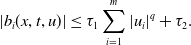 \begin{equation*}|b_i(x,t,u)|\leq \tau _1\sum _{i=1}^m|u_i|^q+\tau _2.\end{equation*}
Under assumptions (I) and (II), we conclude the results in [Reference Dung12, Theorem 1] and [Reference Du and Peng11, Lemma 2.1] in the following lemma.
Lemma 2.1.
Let $p_0$
be a positive constant such that
$p_0$
be a positive constant such that $p_0\gt \frac {n}{2}\max \{0,q-1\}$
and
$p_0\gt \frac {n}{2}\max \{0,q-1\}$
and $T(u^0)$
be the maximal existence time of the solution
$T(u^0)$
be the maximal existence time of the solution $u$
satisfying (
2.1
) corresponding to the initial data
$u$
satisfying (
2.1
) corresponding to the initial data $u^0$
. Suppose that there exists a positive constant
$u^0$
. Suppose that there exists a positive constant $C_{p_0}$
depending on the initial data such that
$C_{p_0}$
depending on the initial data such that $\|u(\cdot ,t)\|_{L^{p_0}(\Omega )}\leq C_{p_0}(u^0)$
for all
$\|u(\cdot ,t)\|_{L^{p_0}(\Omega )}\leq C_{p_0}(u^0)$
for all $t\in (0,T(u^0))$
, then the solution
$t\in (0,T(u^0))$
, then the solution $u$
exists for all time, and there is a positive constant
$u$
exists for all time, and there is a positive constant $C_{\infty }(u^0)$
such that
$C_{\infty }(u^0)$
such that $\|u(\cdot ,t)\|_{L^\infty (\Omega )}\leq C_\infty (u^0)$
for all
$\|u(\cdot ,t)\|_{L^\infty (\Omega )}\leq C_\infty (u^0)$
for all $t\in (0,\infty )$
.
$t\in (0,\infty )$
.
Moreover, suppose that there exist finite numbers $\varrho$
and
$\varrho$
and $K_{p_0}(\varrho)$
independent of the initial data such that
$K_{p_0}(\varrho)$
independent of the initial data such that $\|u(\cdot ,t)\|_{L^{p_0}(\Omega )}\leq K_{p_0}(\varrho )$
for all
$\|u(\cdot ,t)\|_{L^{p_0}(\Omega )}\leq K_{p_0}(\varrho )$
for all $t\in [\varrho ,\infty )$
, then there is a positive number
$t\in [\varrho ,\infty )$
, then there is a positive number $K_{\infty }(\varrho )$
independent of the initial data such that
$K_{\infty }(\varrho )$
independent of the initial data such that $\|u(\cdot ,t)\|_{L^\infty (\Omega )}\leq K_{\infty }(\varrho )$
for
$\|u(\cdot ,t)\|_{L^\infty (\Omega )}\leq K_{\infty }(\varrho )$
for $t\in [\varrho ,\infty )$
.
$t\in [\varrho ,\infty )$
.
By virtue of Lemma2.1, we can demonstrate the boundedness of the solution to (1.5).
Theorem 2.1.
Assume that (H1)–(H4) hold. There exists a positive constant $N_1$
depending on the initial data such that the nonnegative solution
$N_1$
depending on the initial data such that the nonnegative solution $(S,I)$
of (
1.5
) satisfies
$(S,I)$
of (
1.5
) satisfies
 \begin{equation*}\|S(\cdot ,t)\|_{L^\infty (\Omega )}+\|I(\cdot ,t)\|_{L^\infty (\Omega )}\leq N_1,\ \forall \ t\in (0,\infty ).\end{equation*}
Moreover, there exists a positive constant $N_2$
independent of the initial data such that
$N_2$
independent of the initial data such that
 \begin{equation*}\|S(\cdot ,t)\|_{L^\infty (\Omega )}+\|I(\cdot ,t)\|_{L^\infty (\Omega )}\leq N_2,\ \forall \ t\in [T,\infty ),\end{equation*}
for some large time $T\gt 0$
.
$T\gt 0$
.

2.2. Boundedness for the Fokker–Planck-type diffusion
In this subsection, we assume $S_0\in C(\bar {\Omega })$
and
$S_0\in C(\bar {\Omega })$
and $I_0\in W^{1,\infty }(\Omega )$
for (1.6). Building on the classical results of Amann [Reference Amann2–Reference Amann4] on the local existence of solutions for quasilinear parabolic equations, we present the following preliminary result regarding the local existence of solutions for (1.6).
$I_0\in W^{1,\infty }(\Omega )$
for (1.6). Building on the classical results of Amann [Reference Amann2–Reference Amann4] on the local existence of solutions for quasilinear parabolic equations, we present the following preliminary result regarding the local existence of solutions for (1.6).
Lemma 2.2.
Assume that (H1)–(H4) hold. There exists $T_{\max }\in (0,\infty ]$
and a uniquely determined pair of nonnegative functions
$T_{\max }\in (0,\infty ]$
and a uniquely determined pair of nonnegative functions
 \begin{equation*}S\in C(\bar {\Omega }\times [0,T_{\max }))\cap C^{2,1}(\bar {\Omega }\times (0,T_{\max })),\end{equation*}
 \begin{equation*}I\in C(\bar {\Omega }\times [0,T_{\max }))\cap C^{2,1}(\bar {\Omega }\times (0,T_{\max }))\cap L_{\mathrm{loc}}^\infty ([0,T_{\max });\,W^{1,p}(\Omega )),\end{equation*}
with any $p\gt 1$
such that
$p\gt 1$
such that $(S,I)$
solves (
1.6
) classically in
$(S,I)$
solves (
1.6
) classically in $\Omega \times (0,T_{\max })$
. Furthermore, if
$\Omega \times (0,T_{\max })$
. Furthermore, if $T_{\max }\lt \infty$
, then for any
$T_{\max }\lt \infty$
, then for any $p\gt 1$
,
$p\gt 1$
,
 \begin{equation*}\|S(\cdot ,t)\|_{L^\infty (\Omega )}+\|I(\cdot ,t)\|_{W^{1,p}(\Omega )}\rightarrow \infty , \mathrm {as}\ t\nearrow T_{\max }.\end{equation*}
The following lemma establishes the $W^{1,\infty }(\Omega )$
boundedness of
$W^{1,\infty }(\Omega )$
boundedness of $I$
for every
$I$
for every $t\in (0,T_{\max })$
.
$t\in (0,T_{\max })$
.
Lemma 2.3.
Assume that (H1)–(H4) hold and $\gamma$
is constant. Then, there exist positive constants
$\gamma$
is constant. Then, there exist positive constants $M_1$
and
$M_1$
and $M_2$
depending on
$M_2$
depending on $\Omega ,n,\beta ,\gamma ,k,\eta$
and
$\Omega ,n,\beta ,\gamma ,k,\eta$
and $N$
such that
$N$
such that
 \begin{equation} \|I(\cdot ,t)\|_{L^\infty (\Omega )}\leq M_1,\ \forall \ t\in (0,T_{\max }), \end{equation}
and
 \begin{equation} \|\nabla I(\cdot ,t)\|_{L^\infty (\Omega )}\leq M_2,\ \forall \ t\in (0,T_{\max }). \end{equation}
Proof. Due to (1.9), we can apply Lemma2.1 with $q=p_0=1$
to the
$q=p_0=1$
to the $I$
-equation in (1.6) to yield a positive constant
$I$
-equation in (1.6) to yield a positive constant $M_1$
independent of
$M_1$
independent of $t$
such that (2.2) holds. According to the variation-of-constants formula, we obtain
$t$
such that (2.2) holds. According to the variation-of-constants formula, we obtain
 \begin{equation} I(\cdot ,t)=e^{tg\Delta }I_0+\int _0^t e^{(t-s)g\Delta }\left (\frac {\beta SI}{S+I}-\gamma I\right )(\cdot ,s)ds,\ \forall \ t\in (0,T_{\max }). \end{equation}
We calculate the gradient for the both sides of (2.4) and consider the $L^\infty$
norm to get
$L^\infty$
norm to get
 \begin{eqnarray*} \|\nabla I(\cdot ,t)\|_{L^\infty (\Omega )}&&\leq \|\nabla e^{tg\Delta }I_0\|_{L^\infty (\Omega )} \\ && \quad +\int _0^t\left \|\nabla e^{(t-s)g\Delta }(\beta +\gamma )I(\cdot ,s)\right \|_{L^\infty (\Omega )}ds,\ \forall \ t\in (0,T_{\max }). \end{eqnarray*}
Let $\lambda _1\,:\!=\,\lambda _1(g)\gt 0$
be the first positive eigenvalue of
$\lambda _1\,:\!=\,\lambda _1(g)\gt 0$
be the first positive eigenvalue of $-g\Delta$
with homogeneous Neumann boundary condition. Then, by the smoothing properties of the Neumann heat semigroup [Reference Winkler31, Lemma 1.3] and (2.2), we have
$-g\Delta$
with homogeneous Neumann boundary condition. Then, by the smoothing properties of the Neumann heat semigroup [Reference Winkler31, Lemma 1.3] and (2.2), we have
 \begin{eqnarray*} \|\nabla I(\cdot ,t)\|_{L^\infty (\Omega )}&\leq &C_1\|I_0\|_{W^{1,\infty }(\Omega )}+C_2\int _0^t(1+(t-s)^{-\frac {1}{2}})e^{-\lambda _1g(t-s)}\|I(\cdot ,s)\|_{L^\infty (\Omega )}ds, \\ &\leq &C_3,\ \forall \ t\in (0,T_{\max }), \end{eqnarray*}
where $C_1$
,
$C_1$
, $C_2$
and
$C_2$
and $C_3$
are positive constants independent of
$C_3$
are positive constants independent of $T_{\max }$
. This results in (2.3).
$T_{\max }$
. This results in (2.3).
Building upon the boundedness of $I$
and
$I$
and $\nabla I$
, we turn to obtain the
$\nabla I$
, we turn to obtain the $L^p$
estimate of
$L^p$
estimate of $S$
.
$S$
.
Lemma 2.4.
Assume that (H1)–(H4) hold and $\gamma$
is constant. For any
$\gamma$
is constant. For any $p\gt 1$
, we have the following estimate
$p\gt 1$
, we have the following estimate
 \begin{equation*} \|S(\cdot ,t)\|_{L^p(\Omega )}\leq C,\ \forall \ t\in (0,T_{\max }). \end{equation*}
where $C$
is a positive constant independent of
$C$
is a positive constant independent of $t$
.
$t$
.
Proof. We first prove by induction that the lemma holds for $2^k$
for all integers
$2^k$
for all integers $k\geq 0$
, i.e.,
$k\geq 0$
, i.e.,
 \begin{equation} \|S(\cdot ,t)\|_{L^{2^k}(\Omega )}^{2^k}\leq M_{2^k},\ \forall \ t\in (0,T_{\max }), \end{equation}
where $M_{2^k}$
is a positive constant independent of
$M_{2^k}$
is a positive constant independent of $t$
. It follows from (1.9) that (2.5) holds with
$t$
. It follows from (1.9) that (2.5) holds with $M_1=N$
for
$M_1=N$
for $k=0$
. Let
$k=0$
. Let $k\geq 1$
. Suppose that there exists a positive constant
$k\geq 1$
. Suppose that there exists a positive constant $M_{2^{k-1}}$
independent of
$M_{2^{k-1}}$
independent of $t$
such that
$t$
such that
 \begin{equation} \|S(\cdot ,t)\|_{L^{2^{k-1}}(\Omega )}^{2^{k-1}}\leq M_{2^{k-1}},\ \forall \ t\in (0,T_{\max }). \end{equation}
We multiply the first equation in (1.6) by $S^{2^k-1}$
and integrate by parts to produce
$S^{2^k-1}$
and integrate by parts to produce
 \begin{eqnarray*} \frac {1}{2^k}\frac {d}{dt}\int _\Omega S^{2^k}dx&=&\int _\Omega [\nabla \cdot (f\nabla S)+\nabla \cdot (S\nabla f)]S^{2^k-1}dx-\int _\Omega \frac {\beta SI}{S+I}S^{2^k-1}dx+\gamma \int _\Omega IS^{2^k-1}dx\\ &\leq &-\int _\Omega f\nabla S\cdot \nabla S^{2^k-1}dx-\int _\Omega S\nabla f\cdot \nabla S^{2^k-1}dx+\gamma \int _\Omega IS^{2^k-1}dx\\ &=&-\,(2^k-1)\int _\Omega fS^{2^k-2}|\nabla S|^2-(2^k-1)\int _\Omega f_S S^{2^k-1}|\nabla S|^2dx\\ &&-\,(2^k-1)\int _\Omega \big(f_\beta S^{2^k-1}\nabla \beta \cdot \nabla S+f_I S^{2^k-1}\nabla I\cdot \nabla S\big)dx\\ &&+\,\gamma \int _\Omega I S^{2^k-1}dx,\ \forall \ t\in (0,T_{\max }). \end{eqnarray*}
Rearranging the above inequality, one has
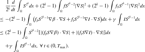 \begin{eqnarray} &&\frac {1}{2^k}\frac {d}{dt}\int _\Omega S^{2^k}dx+(2^k-1)\int _\Omega f S^{2^k-2}|\nabla S|^2+(2^k-1)\int _\Omega f_S S^{2^k-1}|\nabla S|^2dx\nonumber \\ &\leq &-(2^k-1)\int _\Omega \big(f_\beta S^{2^k-1}\nabla \beta \cdot \nabla S+f_I S^{2^k-1}\nabla I\cdot \nabla S\big)dx+\gamma \int _\Omega I S^{2^k-1}dx\nonumber \\ &\leq &(2^k-1)\int _\Omega S^{2^k-2}[|(f_\beta S\nabla \beta )\cdot \nabla S|+|(f_I S\nabla I)\cdot \nabla S|]dx\nonumber \\ &&+\gamma \int _\Omega I S^{2^k-1}dx,\ \forall \ t\in (0,T_{\max }). \end{eqnarray}
By Young’s inequality, we can obtain
 \begin{equation} |(f_\beta S\nabla \beta )\cdot \nabla S|\leq \frac {f}{4}|\nabla S|^2+\frac {f_\beta ^2|\nabla \beta |^2 S^2}{f} \end{equation}
and
 \begin{equation} |(f_I S\nabla I)\cdot \nabla S|\leq \frac {f}{4}|\nabla S|^2+\frac {f_I^2|\nabla I|^2 S^2}{f}. \end{equation}
For any $\epsilon _1\gt 0$
, an application of Young’s inequality again to the last term on the right-hand side of (2.7) gives
$\epsilon _1\gt 0$
, an application of Young’s inequality again to the last term on the right-hand side of (2.7) gives
 \begin{equation} \int _\Omega I S^{2^k-1}dx\leq \|I(\cdot ,t)\|_{L^\infty (\Omega )}\left (\epsilon _1\int _\Omega S^{2^k} dx+C_{\epsilon _1}|\Omega |\right ),\ \forall \ t\in (0,T_{\max }), \end{equation}
where $C_{\epsilon _1}$
is a positive constant depending on
$C_{\epsilon _1}$
is a positive constant depending on $\epsilon _1$
. By Lemma2.3, there exists a positive constant
$\epsilon _1$
. By Lemma2.3, there exists a positive constant $K$
depending on
$K$
depending on $M_1$
such that
$M_1$
such that $f_\beta ,f_I\leq K$
for all
$f_\beta ,f_I\leq K$
for all $t\in (0,T_{\max })$
. We substitute (2.8)–(2.10) into (2.7) to yield
$t\in (0,T_{\max })$
. We substitute (2.8)–(2.10) into (2.7) to yield
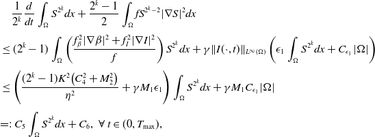 \begin{align} &\quad \frac {1}{2^k}\frac {d}{dt}\int _\Omega S^{2^k}dx+\frac {2^k-1}{2}\int _\Omega f S^{2^k-2}|\nabla S|^2dx\nonumber \\[3pt] &\leq (2^k-1)\int _\Omega \left ( \frac {f_\beta ^2|\nabla \beta |^2+f_I^2|\nabla I|^2}{f}\right )S^{2^k}dx+\gamma \|I(\cdot ,t)\|_{L^\infty (\Omega )}\left (\epsilon _1\int _\Omega S^{2^k} dx+C_{\epsilon _1}|\Omega |\right )\nonumber \\[3pt] &\leq \left (\frac {(2^k-1)K^2\big(C_4^2+M_2^2\big)}{\eta ^2}+\gamma M_1\epsilon _1\right )\int _\Omega S^{2^k} dx+\gamma M_1C_{\epsilon _1}|\Omega |\nonumber \\[3pt] &\!=\!:\, C_5\int _\Omega S^{2^k} dx+C_6,\ \forall \ t\in (0,T_{\max }), \end{align}
where we assume $\|\nabla \beta \|_{L^\infty (\Omega )}\leq C_4$
for a positive constant
$\|\nabla \beta \|_{L^\infty (\Omega )}\leq C_4$
for a positive constant $C_4$
in view of the fact that
$C_4$
in view of the fact that $\beta \in C^1(\bar {\Omega })$
. An application of the interpolation inequality gives that for any
$\beta \in C^1(\bar {\Omega })$
. An application of the interpolation inequality gives that for any $\epsilon _2\gt 0$
,
$\epsilon _2\gt 0$
,
 \begin{equation} \int _\Omega S^{2^k} dx \leq \epsilon _2 \int _\Omega |\nabla S^{2^k-1}|^2 dx +C_{\epsilon _2} \left(\int _\Omega S^{2^{k-1}}dx \right)^2,\ \forall \ t\in (0,T_{\max }). \end{equation}
We now add $\int _\Omega S^{2^k}dx$
to both sides of (2.11) to derive that
$\int _\Omega S^{2^k}dx$
to both sides of (2.11) to derive that
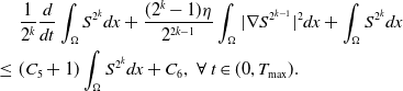 \begin{eqnarray} & &\frac {1}{2^k}\frac {d}{dt}\int _\Omega S^{2^k}dx+\frac {(2^k-1)\eta }{2^{2k-1}}\int _\Omega |\nabla S^{2^{k-1}}|^2dx+\int _\Omega S^{2^k}dx\nonumber \\ &\leq & (C_5+1)\int _\Omega S^{2^k}dx+C_6,\ \forall \ t\in (0,T_{\max }). \end{eqnarray}
Substituting $\epsilon _2 = \frac {(2^k-1)\eta }{2(C_5+1)2^{2k-1}}$
into (2.12) and applying the result to (2.13), we obtain that
$\epsilon _2 = \frac {(2^k-1)\eta }{2(C_5+1)2^{2k-1}}$
into (2.12) and applying the result to (2.13), we obtain that
 \begin{eqnarray} & &\frac {1}{2^k}\frac {d}{dt}\int _\Omega S^{2^k}dx+\frac {(2^k-1)\eta }{2^{2k}}\int _\Omega |\nabla S^{2^{k-1}}|^2dx+\int _\Omega S^{2^k}dx\nonumber \\ &\leq & (C_5+1)C_{\epsilon _2}\left(\int _\Omega S^{2^{k-1}}dx \right)^2+C_6, \ \forall \ t\in (0,T_{\max }). \end{eqnarray}
It follows from (2.6) that
 \begin{equation*} \frac {1}{2^k}\frac {d}{dt}\int _\Omega S^{2^k}dx+\frac {(2^k-1)\eta }{4}\int _\Omega |\nabla S^{2^{k-1}}|^2dx+\int _\Omega S^{2^k}dx\leq C_7, \ \forall \ t\in (0,T_{\max }). \end{equation*}
By means of the Gronwall’s inequality, one infers that (2.5) holds.
By virtue of (2.5) and the embedding $L^{k_1}(\Omega )\subset L^{k_2}(\Omega )$
for any
$L^{k_1}(\Omega )\subset L^{k_2}(\Omega )$
for any $k_1\gt k_2\geq 1$
, we then conclude the lemma holds.
$k_1\gt k_2\geq 1$
, we then conclude the lemma holds.
Lemma 2.5.
Assume that (H1)–(H4) hold and $\gamma$
is constant. There exists a positive constant
$\gamma$
is constant. There exists a positive constant $C$
independent of
$C$
independent of $t$
such that
$t$
such that
 \begin{equation*} \|S(\cdot ,t)\|_{L^\infty (\Omega )}\leq C,\ \forall \ t\in (0,T_{\max }). \end{equation*}
Proof. It follows from the standard Moser-type iteration procedure [Reference Tao and Winkler26, Lemma A.1] that the lemma holds as $p$
can be chosen large enough in Lemma2.4.
$p$
can be chosen large enough in Lemma2.4.
Combining Lemmas2.2 and 2.5 yields $T_{\max }=\infty$
. We are ready to state the boundedness of the solution to (1.6).
$T_{\max }=\infty$
. We are ready to state the boundedness of the solution to (1.6).
Theorem 2.2.
Assume that (H1)–(H4) hold and $\gamma$
is constant. (
1.6
) possesses a global classical solution
$\gamma$
is constant. (
1.6
) possesses a global classical solution
 \begin{equation*}S\in C(\bar {\Omega }\times [0,\infty ))\cap C^{2,1}(\bar {\Omega }\times (0,\infty )),\end{equation*}
 \begin{equation*}I\in C(\bar {\Omega }\times [0,\infty ))\cap C^{2,1}(\bar {\Omega }\times (0,\infty ))\cap L_{\mathrm{loc}}^\infty ([0,\infty );\,W^{1,\infty }(\Omega )),\end{equation*}
such that both $S$
and
$S$
and $I$
are nonnegative in
$I$
are nonnegative in $\bar {\Omega }\times (0,\infty )$
. In addition, there exists a positive constant
$\bar {\Omega }\times (0,\infty )$
. In addition, there exists a positive constant $C$
depending on
$C$
depending on $N$
such that
$N$
such that
 \begin{equation} \|S(\cdot ,t)\|_{L^\infty (\Omega )}+\|I(\cdot ,t)\|_{W^{1,\infty }(\Omega )}\leq C,\ \forall \ t\in (0,\infty ). \end{equation}
3. Spectrum analysis
The constant $k$
in the diffusion rates of the infected population serves as a key parameter that governs the sensitivity of their mobility to the recovery rate. In particular, a larger
$k$
in the diffusion rates of the infected population serves as a key parameter that governs the sensitivity of their mobility to the recovery rate. In particular, a larger $k$
corresponds to a stronger reduction in movement as recovery progresses. This coupling between recovery and mobility directly influences the basic reproduction number, a threshold quantity that usually determines whether an infectious disease will persist or eventually die out. Therefore, analysing the monotonicity and asymptotic behaviour of the basic reproduction number with respect to
$k$
corresponds to a stronger reduction in movement as recovery progresses. This coupling between recovery and mobility directly influences the basic reproduction number, a threshold quantity that usually determines whether an infectious disease will persist or eventually die out. Therefore, analysing the monotonicity and asymptotic behaviour of the basic reproduction number with respect to $k$
is essential. Such analysis provides a theoretical foundation for evaluating the effectiveness of non-pharmaceutical interventions, such as mobility restrictions, in controlling or mitigating disease spread. In this section, we focus on the monotonicity and asymptotics of the principal eigenvalues and basic reproduction numbers in terms of the parameter
$k$
is essential. Such analysis provides a theoretical foundation for evaluating the effectiveness of non-pharmaceutical interventions, such as mobility restrictions, in controlling or mitigating disease spread. In this section, we focus on the monotonicity and asymptotics of the principal eigenvalues and basic reproduction numbers in terms of the parameter $k$
for (1.5) and (1.6). If the diffusion rate
$k$
for (1.5) and (1.6). If the diffusion rate $g$
of infected individuals exponentially or algebraically depends on the recovery rate, we write
$g$
of infected individuals exponentially or algebraically depends on the recovery rate, we write $g(\gamma )=\eta d(k;\,\gamma )$
with
$g(\gamma )=\eta d(k;\,\gamma )$
with $d(k;\,\gamma )=e^{-k\gamma }$
or
$d(k;\,\gamma )=e^{-k\gamma }$
or $d(k;\,\gamma )=(1+\gamma )^{-k}$
, where
$d(k;\,\gamma )=(1+\gamma )^{-k}$
, where $d(k;\,\gamma )$
is monotone decreasing with respect to
$d(k;\,\gamma )$
is monotone decreasing with respect to $k$
for
$k$
for $k\in (0,\infty )$
, i.e.,
$k\in (0,\infty )$
, i.e., $d^{\prime}(k;\,\gamma )\leq 0$
. We further add the following assumption.
$d^{\prime}(k;\,\gamma )\leq 0$
. We further add the following assumption.
(H5) $f(\beta ,S,0)=\eta$
and
$f(\beta ,S,0)=\eta$
and $\lim _{k\rightarrow 0} \eta d(k;\,\gamma )=\eta$
.
$\lim _{k\rightarrow 0} \eta d(k;\,\gamma )=\eta$
.
It follows from Lemma2.1 in [Reference Allen, Bolker, Lou and Nevai1] that the unique DFE of both (1.5) and (1.6) is $\left (\frac {N}{|\Omega |},0\right )$
.
$\left (\frac {N}{|\Omega |},0\right )$
.
3.1. Spectrum for Fickian diffusion
We linearize the $I$
-equation of (1.5) at the DFE to get that
$I$
-equation of (1.5) at the DFE to get that
 \begin{equation} \left \{\begin{aligned} &\partial _t \tilde {I}-\nabla \cdot (g(\gamma )\nabla \tilde {I})=(\beta -\gamma )\tilde {I},\ & x&\in \Omega ,\ t\gt 0,\\ &\displaystyle \nabla \tilde {I}\cdot \mathbf{n}=0,\ & x&\in \partial \Omega ,\ t\gt 0. \end{aligned}\right . \end{equation}
Letting $\tilde {I}(x,t)=e^{-\nu t}\phi (x)$
in (3.1) leads to
$\tilde {I}(x,t)=e^{-\nu t}\phi (x)$
in (3.1) leads to
 \begin{equation} \left \{\begin{aligned} &\nabla \cdot (g(\gamma )\nabla \phi )+(\beta -\gamma )\phi +\nu \phi =0,\ & x&\in \Omega ,\\ &\displaystyle \nabla \phi \cdot \mathbf{n}=0,\ & x&\in \partial \Omega . \end{aligned}\right . \end{equation}
It follows from the Krein–Rutman theorem in [Reference Krein and Rutman14] that (3.2) admits a unique eigenvalue $\nu ^*$
with a positive eigenfunction
$\nu ^*$
with a positive eigenfunction $\phi ^*$
on
$\phi ^*$
on $\Omega$
.
$\Omega$
. $\nu ^*$
is called the principal eigenvalue, which can be described by the variational characterization:
$\nu ^*$
is called the principal eigenvalue, which can be described by the variational characterization:
 \begin{equation} \nu ^*=\inf _{0\neq \phi \in H^1(\Omega )}\left \{\frac {\int _\Omega g(\gamma )|\nabla \phi |^2dx+\int _\Omega (\gamma -\beta )\phi ^2dx}{\int _\Omega \phi ^2dx}\right \}. \end{equation}
For the case of $g(\gamma )=\eta g_1(\gamma )$
, where
$g(\gamma )=\eta g_1(\gamma )$
, where $\eta$
is a positive constant and
$\eta$
is a positive constant and $g_1(\gamma )\gt 0$
is a smooth function, the asymptotic properties of
$g_1(\gamma )\gt 0$
is a smooth function, the asymptotic properties of $\nu ^*$
with respect to
$\nu ^*$
with respect to $\eta$
are given in [Reference Wang, Wang and Kim29, Lemma 2.2].
$\eta$
are given in [Reference Wang, Wang and Kim29, Lemma 2.2].
The exponentially and algebraically dependent diffusion rates are typical examples that satisfy (H5). We consider the asymptotic behaviours of $\nu ^*$
as
$\nu ^*$
as $k\rightarrow 0$
and
$k\rightarrow 0$
and $k\rightarrow \infty$
.
$k\rightarrow \infty$
.
Proposition 3.1.
Assume that (H1)–(H5) hold. Let $\nu ^*\,:\!=\,\nu ^*(\eta d(k;\,\gamma ),\beta -\gamma )$
and
$\nu ^*\,:\!=\,\nu ^*(\eta d(k;\,\gamma ),\beta -\gamma )$
and $\phi ^*\,:\!=\,\phi ^*(\eta d(k;\,\gamma ),$ $\beta -\gamma )$
denote the principal eigenvalue and the corresponding eigenfunction of (
3.2
), respectively. Then, the following results for
$\beta -\gamma )$
denote the principal eigenvalue and the corresponding eigenfunction of (
3.2
), respectively. Then, the following results for $\nu ^*$
hold.
$\nu ^*$
hold.
(i) $\nu ^*$
and
$\nu ^*$
and $\phi ^*$
depend smoothly on parameter
$\phi ^*$
depend smoothly on parameter $k\in (0,\infty )$
. In addition,
$k\in (0,\infty )$
. In addition, $\nu ^*$
is a strictly monotone decreasing function of
$\nu ^*$
is a strictly monotone decreasing function of $k$
if the functions
$k$
if the functions $k\mapsto d(k;\,\gamma )$
and
$k\mapsto d(k;\,\gamma )$
and $\beta -\gamma$
are non-constant.
$\beta -\gamma$
are non-constant.
(ii) $\nu ^*\rightarrow \nu ^*(\eta ,\beta -\gamma )$
, as
$\nu ^*\rightarrow \nu ^*(\eta ,\beta -\gamma )$
, as $k\rightarrow 0$
, where
$k\rightarrow 0$
, where $\nu ^*(\eta ,\beta -\gamma )$
is the principal eigenvalue of
$\nu ^*(\eta ,\beta -\gamma )$
is the principal eigenvalue of
 \begin{equation} \left \{\begin{aligned} &\eta \Delta \phi +(\beta -\gamma )\phi +\nu \phi =0,\ & x&\in \Omega ,\\ &\displaystyle \nabla \phi \cdot \mathbf{n}=0,\ & x&\in \partial \Omega . \end{aligned}\right . \end{equation}
(iii) If $d(k;\,\gamma )=e^{-k\gamma }$
or
$d(k;\,\gamma )=e^{-k\gamma }$
or $d(k;\,\gamma )=(1+\gamma )^{-k}$
, then
$d(k;\,\gamma )=(1+\gamma )^{-k}$
, then $\nu ^*\rightarrow \min _{x\in \bar {\Omega }}\{\gamma -\beta \}$
as
$\nu ^*\rightarrow \min _{x\in \bar {\Omega }}\{\gamma -\beta \}$
as $k\rightarrow \infty$
.
$k\rightarrow \infty$
.
Proof. The smoothness of $\nu ^*$
and
$\nu ^*$
and $\phi ^*$
on
$\phi ^*$
on $k$
in assertion (i) is standard in [Reference Cantrell and Cosner6] via implicit function theorem. It suffices to verify the monotonicity of
$k$
in assertion (i) is standard in [Reference Cantrell and Cosner6] via implicit function theorem. It suffices to verify the monotonicity of $\nu ^*$
with respect to
$\nu ^*$
with respect to $k$
. We differentiate both sides of (3.2) with
$k$
. We differentiate both sides of (3.2) with $\nu =\nu ^*$
and
$\nu =\nu ^*$
and $\phi =\phi ^*$
by
$\phi =\phi ^*$
by $k$
to produce
$k$
to produce
 \begin{equation} \left \{\begin{aligned} &\eta \nabla \cdot [d^{\prime}(k;\,\gamma )\nabla \phi ^*+d(k;\,\gamma )\nabla (\phi ^*)^{\prime}]+(\beta -\gamma )(\phi ^*)^{\prime}+(\nu ^*)^{\prime}\phi ^*+\nu ^*(\phi ^*)^{\prime}=0,\ & x&\in \Omega ,\\ &\displaystyle \nabla (\phi ^*)^{\prime}\cdot \mathbf{n}=0,\ & x&\in \partial \Omega , \end{aligned}\right . \end{equation}
where the prime notation $^{\prime}$
means differentiation by
$^{\prime}$
means differentiation by $k$
. We multiply (3.5) by
$k$
. We multiply (3.5) by $\phi ^*$
and (3.2) with
$\phi ^*$
and (3.2) with $\nu =\nu ^*$
and
$\nu =\nu ^*$
and $\phi =\phi ^*$
by
$\phi =\phi ^*$
by $(\phi ^*)^{\prime}$
, subtract the results and integrate by parts over
$(\phi ^*)^{\prime}$
, subtract the results and integrate by parts over $\Omega$
to yield
$\Omega$
to yield
 \begin{equation*} (\nu ^*)^{\prime}\int _\Omega (\phi ^*)^2dx=\eta \int _\Omega d^{\prime}(k;\,\gamma )|\nabla \phi ^*|^2dx. \end{equation*}
It follows from $d^{\prime}(k;\,\gamma )\leq 0$
that
$d^{\prime}(k;\,\gamma )\leq 0$
that $(\nu ^*)^{\prime}\leq 0$
. Since
$(\nu ^*)^{\prime}\leq 0$
. Since $k\mapsto d(k;\,\gamma )$
is non-constant, we find that the equality holds only if
$k\mapsto d(k;\,\gamma )$
is non-constant, we find that the equality holds only if $\phi ^*$
is constant on
$\phi ^*$
is constant on $\Omega$
. Then, by (3.2), we get
$\Omega$
. Then, by (3.2), we get
 \begin{equation*} \beta -\gamma +\nu ^*=0,\ x\in \Omega . \end{equation*}
This leads to a contradiction as $\beta -\gamma$
is non-constant on
$\beta -\gamma$
is non-constant on $\Omega$
. Hence,
$\Omega$
. Hence, $\nu ^*\lt 0$
.
$\nu ^*\lt 0$
.
It follows from (i) and (H5) that assertion (ii) holds. We turn to prove (iii). According to (3.3), one has
 \begin{eqnarray} \nu ^*\geq \inf _{0\neq \phi \in H^1(\Omega )}\left \{\frac {\int _{\Omega }(\gamma -\beta )\phi ^2dx}{\int _\Omega \phi ^2dx}\right \} \geq \min _{x\in \bar {\Omega }}\{\gamma -\beta \}. \end{eqnarray}
For any $\epsilon$
, we can choose
$\epsilon$
, we can choose $\phi _\epsilon \in H^1(\Omega )$
such that
$\phi _\epsilon \in H^1(\Omega )$
such that
 \begin{equation*}\gamma -\beta \leq \min _{x\in \bar {\Omega }}\{\gamma -\beta \}+\epsilon ,\ \forall \ x\in \ \mathrm{supp}(\phi _\epsilon ).\end{equation*}
We find that
 \begin{eqnarray*} \lim _{k\rightarrow \infty }\nu ^*&\leq &\lim _{k\rightarrow \infty } \frac {\eta \int _{\mathrm{supp}(\phi _\epsilon )}d(k;\,\gamma )|\nabla \phi _\epsilon |^2dx+\int _{\mathrm{supp}(\phi _\epsilon )} (\gamma -\beta )\phi _\epsilon ^2 dx}{\int _{\mathrm{supp}(\phi _\epsilon )}\phi _\epsilon ^2dx}\\ &\leq &\min _{x\in \bar {\Omega }}\{\gamma -\beta \}+\epsilon . \end{eqnarray*}
This together with (3.6) and the arbitrariness of $\epsilon$
gives (iii).
$\epsilon$
gives (iii).
We then consider the corresponding eigenvalue problem with the weight $\beta$
for (1.5)
$\beta$
for (1.5)
 \begin{equation} \left \{\begin{aligned} &\!-\nabla \cdot (g(\gamma )\nabla \psi )+\gamma \psi =\nu \beta \psi ,\ & x&\in \Omega ,\\ &\displaystyle \nabla \psi \cdot \mathbf{n}=0,\ & x&\in \partial \Omega . \end{aligned}\right . \end{equation}
The principal eigenvalue of (3.7) can also be given by the variational characterization
 \begin{equation*}\nu _0=\inf _{0\neq \psi \in H^1(\Omega )}\left \{\frac {\int _\Omega g(\gamma )|\nabla \psi |^2dx+\int _\Omega \gamma \psi ^2 dx}{\int _\Omega \beta \psi ^2dx}\right \}\!.\end{equation*}
Then, the basic reproduction for (1.5) $\mathcal{R}_0$
(1.5) can be defined as the inverse of
$\mathcal{R}_0$
(1.5) can be defined as the inverse of $\nu _0$
:
$\nu _0$
:
 \begin{equation*}\mathcal{R}_0^{(1.5)}(g(\gamma ),\beta ,\gamma )=\frac {1}{\nu _0}=\sup _{0\neq \psi \in H^1(\Omega )}\left \{\frac {\int _\Omega \beta \psi ^2dx}{\int _\Omega g(\gamma )|\nabla \psi |^2dx+\int _\Omega \gamma \psi ^2 dx}\right \}\!.\end{equation*}
By inspection of $\mathcal{R}_0$
(1.5), we get the following properties.
$\mathcal{R}_0$
(1.5), we get the following properties.
Proposition 3.2.
Assume that (H1)–(H5) hold. Let $\mathcal{R}_0$
(1.5)
$\mathcal{R}_0$
(1.5) $:\!=\,\mathcal{R}_0$
(1.5)
$:\!=\,\mathcal{R}_0$
(1.5) $(\eta d(k;\,\gamma ),\beta ,\gamma )$
denote the basic reproduction number of (1.5).
$(\eta d(k;\,\gamma ),\beta ,\gamma )$
denote the basic reproduction number of (1.5). $\mathcal{R}_0$
(1.5) satisfies the following properties.
$\mathcal{R}_0$
(1.5) satisfies the following properties.
(i) $\mathcal{R}_0$
(1.5) depends smoothly on parameter
$\mathcal{R}_0$
(1.5) depends smoothly on parameter $k\in (0,\infty )$
and is a monotone increasing function of
$k\in (0,\infty )$
and is a monotone increasing function of $k$
.
$k$
.
(ii) $\mathcal{R}_0$
(1.5)
$\mathcal{R}_0$
(1.5) $\rightarrow \mathcal{R}_0$
(1.5)
$\rightarrow \mathcal{R}_0$
(1.5) $(\eta ,\beta ,\gamma )$
, as
$(\eta ,\beta ,\gamma )$
, as $k\rightarrow 0$
, where
$k\rightarrow 0$
, where $\mathcal{R}_0$
(1.5)
$\mathcal{R}_0$
(1.5) $(\eta ,\beta ,\gamma )$
fulfils the following problem:
$(\eta ,\beta ,\gamma )$
fulfils the following problem:
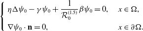 \begin{equation} \left \{\begin{aligned} &\eta \Delta \psi _0-\gamma \psi _0+\frac {1}{\mathcal{R}_0^{(1.5)}}\beta \psi _0=0,\ & x&\in \Omega ,\\ &\displaystyle \nabla \psi _0\cdot \mathbf{n}=0,\ & x&\in \partial \Omega . \end{aligned}\right . \end{equation}
(iii) If $d(k;\,\gamma )=e^{-k\gamma }$
or
$d(k;\,\gamma )=e^{-k\gamma }$
or $d(k;\,\gamma )=(1+\gamma )^{-k}$
, then
$d(k;\,\gamma )=(1+\gamma )^{-k}$
, then $\mathcal{R}_0$
(1.5)
$\mathcal{R}_0$
(1.5) $\rightarrow \max _{x\in \bar {\Omega }}\{\beta /\gamma \}$
as
$\rightarrow \max _{x\in \bar {\Omega }}\{\beta /\gamma \}$
as $k\rightarrow \infty$
.
$k\rightarrow \infty$
.
3.2. Spectrum for the Fokker–Planck-type diffusion
Now we explore the eigenvalue problems of (1.6). Linearizing the $I$
-equation of (1.6) at the DFE gives
$I$
-equation of (1.6) at the DFE gives
 \begin{equation} \left \{\begin{aligned} &\partial _t \tilde {I}-\Delta (g(\gamma )\tilde {I})=(\beta -\gamma )\tilde {I},\ & x&\in \Omega ,\ t\gt 0,\\ &\displaystyle \nabla (g(\gamma )\tilde {I})\cdot \mathbf{n}=0,\ & x&\in \partial \Omega ,\ t\gt 0. \end{aligned}\right . \end{equation}
Letting $\tilde {I}(x,t)=e^{-\mu t}\varphi (x)$
in (3.9) results in
$\tilde {I}(x,t)=e^{-\mu t}\varphi (x)$
in (3.9) results in
 \begin{equation} \left \{\begin{aligned} &\Delta (g(\gamma )\varphi )+(\beta -\gamma )\varphi +\mu \varphi =0,\ & x&\in \Omega ,\\ &\displaystyle \nabla (g(\gamma )\varphi )\cdot \mathbf{n}=0,\ & x&\in \partial \Omega . \end{aligned}\right . \end{equation}
Setting $\Phi (x)=g(\gamma )\varphi (x)$
, (3.10) becomes
$\Phi (x)=g(\gamma )\varphi (x)$
, (3.10) becomes
 \begin{equation} \left \{\begin{aligned} &g(\gamma )\Delta \Phi +(\beta -\gamma )\Phi +\mu \Phi =0,\ & x&\in \Omega ,\\ &\displaystyle \nabla \Phi \cdot \mathbf{n}=0,\ & x&\in \partial \Omega . \end{aligned}\right . \end{equation}
In view of the Krein–Rutman theorem [Reference Krein and Rutman14] again, problem (3.11) admits a principal eigenvalue, denoted by $\mu ^*$
, which corresponds to a strictly positive eigenfunction
$\mu ^*$
, which corresponds to a strictly positive eigenfunction $\Phi ^*$
on
$\Phi ^*$
on $\Omega$
. By the variational characterization,
$\Omega$
. By the variational characterization, $\mu ^*$
can be represented by
$\mu ^*$
can be represented by
 \begin{equation*}\mu ^*=\inf _{0\neq \Phi \in H^1(\Omega )}\left \{\frac {\int _\Omega |\nabla \Phi |^2dx+\int _\Omega \frac {\beta -\gamma }{g(\gamma )}\Phi ^2dx}{\int _\Omega \frac {\Phi ^2}{g(\gamma )}dx}\right \}\!.\end{equation*}
When $g(\gamma )=\eta d(k;\,\gamma )$
, we have the following properties of
$g(\gamma )=\eta d(k;\,\gamma )$
, we have the following properties of $\mu ^*$
.
$\mu ^*$
.
Proposition 3.3.
Assume that (H1)–(H5) hold. Let $\mu ^*\,:\!=\,\mu ^*(\eta d(k;\,\gamma ),\beta -\gamma )$
and
$\mu ^*\,:\!=\,\mu ^*(\eta d(k;\,\gamma ),\beta -\gamma )$
and $\Phi ^*\,:\!=\,\Phi ^*(\eta d(k;\,\gamma ),\beta -\gamma )$
denote the principal eigenvalue and the corresponding eigenfunction of (
3.11
), respectively. Then, the following results for
$\Phi ^*\,:\!=\,\Phi ^*(\eta d(k;\,\gamma ),\beta -\gamma )$
denote the principal eigenvalue and the corresponding eigenfunction of (
3.11
), respectively. Then, the following results for $\mu ^*$
hold.
$\mu ^*$
hold.
(i) $\mu ^*$
and
$\mu ^*$
and $\Phi ^*$
depend smoothly on parameter
$\Phi ^*$
depend smoothly on parameter $k\in (0,\infty )$
. In addition,
$k\in (0,\infty )$
. In addition, $\mu ^*$
is a strictly monotone decreasing function of
$\mu ^*$
is a strictly monotone decreasing function of $k$
if the functions
$k$
if the functions $k\mapsto d(k;\,\gamma )$
and
$k\mapsto d(k;\,\gamma )$
and $\beta -\gamma$
are non-constant.
$\beta -\gamma$
are non-constant.
(ii) $\mu ^*\rightarrow \mu ^*(\eta ,\beta -\gamma )=\nu ^*(\eta ,\beta -\gamma )$
fulfilling problem (
3.4
) as
$\mu ^*\rightarrow \mu ^*(\eta ,\beta -\gamma )=\nu ^*(\eta ,\beta -\gamma )$
fulfilling problem (
3.4
) as $k\rightarrow 0$
.
$k\rightarrow 0$
.
(iii) If $d(k;\,\gamma )=e^{-k\gamma }$
or
$d(k;\,\gamma )=e^{-k\gamma }$
or $d(k;\,\gamma )=(1+\gamma )^{-k}$
, then
$d(k;\,\gamma )=(1+\gamma )^{-k}$
, then $\mu ^*\rightarrow \min _{x\in \bar {\Omega }}\{\gamma -\beta \}$
as
$\mu ^*\rightarrow \min _{x\in \bar {\Omega }}\{\gamma -\beta \}$
as $k\rightarrow \infty$
.
$k\rightarrow \infty$
.
Proof. The proof is similar to that of Proposition3.1, and hence we omit it.
We also consider the eigenvalue problem with the weight for (1.6) as follows:
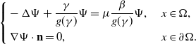 \begin{equation} \left \{\begin{aligned} &\!-\Delta \Psi +\frac {\gamma }{g(\gamma )}\Psi =\mu \frac {\beta }{g(\gamma )}\Psi ,\ & x&\in \Omega ,\\ &\displaystyle \nabla \Psi \cdot \mathbf{n}=0,\ & x&\in \partial \Omega . \end{aligned}\right . \end{equation}
The corresponding principal eigenvalue of (3.12) can also be given via the variational characterization
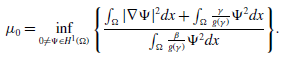 \begin{equation*}\mu _0=\inf _{0\neq \Psi \in H^1(\Omega )}\left \{\frac {\int _\Omega |\nabla \Psi |^2dx+\int _\Omega \frac {\gamma }{g(\gamma )} \Psi ^2 dx}{\int _\Omega \frac {\beta }{g(\gamma )}\Psi ^2dx}\right \}\!.\end{equation*}
Similarly, the basic reproduction number $\mathcal{R}_0$
(1.6) for (1.6) can be characterized as
$\mathcal{R}_0$
(1.6) for (1.6) can be characterized as
 \begin{equation*}\mathcal{R}_0^{(1.6)}(g(\gamma ),\beta ,\gamma )=\frac {1}{\mu _0}=\sup _{0\neq \Psi \in H^1(\Omega )}\left \{\frac {\int _\Omega \frac {\beta }{g(\gamma )}\Psi ^2dx}{\int _\Omega |\nabla \Psi |^2dx+\int _\Omega \frac {\gamma }{g(\gamma )} \Psi ^2 dx}\right \}\!.\end{equation*}
Proposition 3.4.
Assume that (H1)–(H5) hold. Let $\mathcal{R}_0$
(1.6)
$\mathcal{R}_0$
(1.6) $:\!=\,\mathcal{R}_0$
(1.6)
$:\!=\,\mathcal{R}_0$
(1.6) $(\eta d(k;\,\gamma ),\beta ,\gamma )$
denote the basic reproduction number of (
1.6
).
$(\eta d(k;\,\gamma ),\beta ,\gamma )$
denote the basic reproduction number of (
1.6
). $\mathcal{R}_0$
(1.6) satisfies the following properties.
$\mathcal{R}_0$
(1.6) satisfies the following properties.
(i) $\mathcal{R}_0$
(1.6) depends smoothly on parameter
$\mathcal{R}_0$
(1.6) depends smoothly on parameter $k\in (0,\infty )$
and is a monotone increasing function of
$k\in (0,\infty )$
and is a monotone increasing function of $k$
.
$k$
.
(ii) $\mathcal{R}_0$
(1.6)
$\mathcal{R}_0$
(1.6) $\rightarrow \mathcal{R}_0$
(1.6)
$\rightarrow \mathcal{R}_0$
(1.6) $(\eta ,\beta ,\gamma )$
, as
$(\eta ,\beta ,\gamma )$
, as $k\rightarrow 0$
, where
$k\rightarrow 0$
, where $\mathcal{R}_0$
(1.6)
$\mathcal{R}_0$
(1.6) $(\eta ,\beta ,\gamma )$
fulfils the problem (
3.8
).
$(\eta ,\beta ,\gamma )$
fulfils the problem (
3.8
).
(iii) If $d(k;\,\gamma )=e^{-k\gamma }$
or
$d(k;\,\gamma )=e^{-k\gamma }$
or $d(k;\,\gamma )=(1+\gamma )^{-k}$
, then
$d(k;\,\gamma )=(1+\gamma )^{-k}$
, then $\mathcal{R}_0$
(1.6)
$\mathcal{R}_0$
(1.6) $\rightarrow \max _{x\in \bar {\Omega }}\{\beta /\gamma \}$
as
$\rightarrow \max _{x\in \bar {\Omega }}\{\beta /\gamma \}$
as $k\rightarrow \infty$
.
$k\rightarrow \infty$
.
Proof. We only need to verify the monotonicity of $\mathcal{R}_0$
(1.6), as the other properties can be achieved by inspection. We differentiate both sides of (3.12) with
$\mathcal{R}_0$
(1.6), as the other properties can be achieved by inspection. We differentiate both sides of (3.12) with $\mu =\frac {1}{\mathcal{R}_0^{(1.6)}}$
and
$\mu =\frac {1}{\mathcal{R}_0^{(1.6)}}$
and $\Psi =\Psi _0$
by
$\Psi =\Psi _0$
by $k$
to get
$k$
to get
 \begin{equation} \left \{\begin{aligned} &\!-\eta d^{\prime}(k;\,\gamma )\Delta \Psi _0-\eta d(k;\,\gamma )\Delta (\Psi _0)^{\prime}+\gamma (\Psi _0)^{\prime}=-\frac {(\mathcal{R}_0^{(1.6)})^{\prime}}{(\mathcal{R}_0^{(1.6)})^2}\beta \Psi _0+\frac {\beta }{\mathcal{R}_0^{(1.6)}}(\Psi _0)^{\prime},\ & x&\in \Omega ,\\ &\displaystyle \nabla (\Psi _0)^{\prime}\cdot \mathbf{n}=0,\ & x&\in \partial \Omega , \end{aligned}\right . \end{equation}
where $\Psi _0$
is the positive eigenfunction corresponding to
$\Psi _0$
is the positive eigenfunction corresponding to $\mu _0$
. We multiply (3.13) by
$\mu _0$
. We multiply (3.13) by $\Psi _0$
and (3.12) with
$\Psi _0$
and (3.12) with $\mu =\frac {1}{\mathcal{R}_0^{(1.6)}}$
and
$\mu =\frac {1}{\mathcal{R}_0^{(1.6)}}$
and $\Psi =\Psi _0$
by
$\Psi =\Psi _0$
by $(\Psi _0)^{\prime}$
, subtract the results and integrate by parts over
$(\Psi _0)^{\prime}$
, subtract the results and integrate by parts over $\Omega$
to obtain
$\Omega$
to obtain
 \begin{equation*} -\frac {(\mathcal{R}_0^{(1.6)})^{\prime}}{(\mathcal{R}_0^{(1.6)})^2}\int _\Omega \beta (\Psi _0)^2dx=\eta \int _\Omega d^{\prime}(k;\,\gamma )|\nabla \Psi _0|^2dx. \end{equation*}
Since $d^{\prime}(k;\,\gamma )\leq 0$
, one has
$d^{\prime}(k;\,\gamma )\leq 0$
, one has $(\mathcal{R}_0$
(1.6)
$(\mathcal{R}_0$
(1.6) $)^{\prime}\geq 0$
.
$)^{\prime}\geq 0$
.
The parameter $k$
plays an important role in the asymptotic profiles of the basic reproduction number. If
$k$
plays an important role in the asymptotic profiles of the basic reproduction number. If $k\rightarrow 0$
, the limit of the basic reproduction numbers of (1.5) and (1.6) is
$k\rightarrow 0$
, the limit of the basic reproduction numbers of (1.5) and (1.6) is $\mathcal{R}_0$
(1.1) with
$\mathcal{R}_0$
(1.1) with $d_I=\eta$
. The corresponding monotonicity and asymptotics of
$d_I=\eta$
. The corresponding monotonicity and asymptotics of $\mathcal{R}_0$
(1.1) on
$\mathcal{R}_0$
(1.1) on $\eta$
are presented in [Reference Allen, Bolker, Lou and Nevai1, Lemma 2.3]. On the other hand, we find that the basic reproduction numbers of (1.5) and (1.6) have the same limit when
$\eta$
are presented in [Reference Allen, Bolker, Lou and Nevai1, Lemma 2.3]. On the other hand, we find that the basic reproduction numbers of (1.5) and (1.6) have the same limit when $\eta \rightarrow 0$
or
$\eta \rightarrow 0$
or $k\rightarrow \infty$
.
$k\rightarrow \infty$
.
It is difficult to compare $\mathcal{R}_0$
(1.5) and
$\mathcal{R}_0$
(1.5) and $\mathcal{R}_0$
(1.6). However, they are equal when
$\mathcal{R}_0$
(1.6). However, they are equal when $\gamma$
is a positive constant. In this case,
$\gamma$
is a positive constant. In this case,
 \begin{equation*}\mathcal{R}_0^{(1.5)}=\mathcal{R}_0^{(1.6)}=\sup _{0\neq \psi \in H^1(\Omega )}\left \{\frac {\int _\Omega \beta \psi ^2dx}{g(\gamma )\int _\Omega |\nabla \psi |^2dx+\int _\Omega \gamma \psi ^2 dx}\right \}\!,\end{equation*}
as $g(\gamma )$
is also constant.
$g(\gamma )$
is also constant.
4. Threshold dynamics
Linearizing the $S$
-equations of both (1.5) and (1.6) at the DFE leads to the same equation
$S$
-equations of both (1.5) and (1.6) at the DFE leads to the same equation
 \begin{equation} \left \{\begin{aligned} &\partial _t \tilde {S}=\eta \Delta \tilde {S}-(\beta -\gamma )\tilde {I},\ &x&\in \Omega ,\ t\gt 0,\\ & \nabla \tilde {S}\cdot \mathbf{n}=0,\ &x&\in \partial \Omega ,\ t\gt 0, \end{aligned}\right . \end{equation}
where the linearized $\tilde {I}$
is given in (3.1) and (3.9). Note that the diffusion rate of the linearized
$\tilde {I}$
is given in (3.1) and (3.9). Note that the diffusion rate of the linearized $\tilde {S}$
-equation in (4.1) is independent of
$\tilde {S}$
-equation in (4.1) is independent of $\beta$
,
$\beta$
, $\tilde {S}$
and
$\tilde {S}$
and $\tilde {I}$
. It then follows from [Reference Allen, Bolker, Lou and Nevai1, Lemma 2.4] that the magnitude of the basic reproduction number determines the linear stability of the DFE.
$\tilde {I}$
. It then follows from [Reference Allen, Bolker, Lou and Nevai1, Lemma 2.4] that the magnitude of the basic reproduction number determines the linear stability of the DFE.
Proposition 4.1.
If $\mathcal{R}_0$
(1.5)
$\mathcal{R}_0$
(1.5) $\lt 1$
(or
$\lt 1$
(or $\mathcal{R}_0$
(1.6)
$\mathcal{R}_0$
(1.6) $\lt 1$
), then the DFE is stable, while if
$\lt 1$
), then the DFE is stable, while if $\mathcal{R}_0$
(1.5)
$\mathcal{R}_0$
(1.5) $\gt 1$
(or
$\gt 1$
(or $\mathcal{R}_0$
(1.6)
$\mathcal{R}_0$
(1.6) $\gt 1$
), then the DFE is unstable.
$\gt 1$
), then the DFE is unstable.
To explore the stability of EE, we consider the case that either $\beta /\gamma$
is constant for (1.5) or both
$\beta /\gamma$
is constant for (1.5) or both $\beta$
and
$\beta$
and $\gamma$
are spatially homogeneous for (1.6) on
$\gamma$
are spatially homogeneous for (1.6) on $\Omega$
. It can be easily checked that
$\Omega$
. It can be easily checked that $(\hat {S},\hat {I})\,:\!=\,\left (\frac {1}{\mathcal{R}_0 }\frac {N}{|\Omega |},\left (1-\frac {1}{\mathcal{R}_0}\right )\frac {N}{|\Omega |}\right )$
is the unique constant EE, where
$(\hat {S},\hat {I})\,:\!=\,\left (\frac {1}{\mathcal{R}_0 }\frac {N}{|\Omega |},\left (1-\frac {1}{\mathcal{R}_0}\right )\frac {N}{|\Omega |}\right )$
is the unique constant EE, where
 \begin{equation*}\mathcal{R}_0\,:\!=\,\frac {\beta }{\gamma }\end{equation*}
is the basic reproduction number for (1.5) and (1.6). We linearize (1.5) and (1.6) at the constant EE, which leads to
 \begin{equation} \left \{\begin{aligned} &\partial _t \bar {S}=f(\beta ,\hat {S},\hat {I})\Delta \bar {S}-\beta \left (1-\frac {1}{\mathcal{R}_0}\right )^2\bar {S}+\gamma \left (1-\frac {1}{\mathcal{R}_0}\right )\bar {I},\ &x&\in \Omega ,\ t\gt 0,\\ &\partial _t \bar {I}=g(\gamma )\Delta \bar {I}+\beta \left (1-\frac {1}{\mathcal{R}_0}\right )^2\bar {S}-\gamma \left (1-\frac {1}{\mathcal{R}_0}\right )\bar {I},\ &x&\in \Omega ,\ t\gt 0,\\ & \nabla \bar {S}\cdot \mathbf{n}=\nabla \bar {I}\cdot \mathbf{n}=0,\ &x&\in \partial \Omega ,\ t\gt 0. \end{aligned}\right . \end{equation}
The corresponding stability matrix of (4.2) is
 \begin{equation*} \begin{pmatrix} -f(\beta ,\hat {S},\hat {I})l^2-\beta \left (1-\frac {1}{\mathcal{R}_0}\right )^2 & \quad \gamma \left (1-\frac {1}{\mathcal{R}_0}\right )\\[5pt] \beta \left (1-\frac {1}{\mathcal{R}_0}\right )^2 &\quad -g(\gamma ) l^2-\gamma \left (1-\frac {1}{\mathcal{R}_0}\right ) \end{pmatrix}\!, \end{equation*}
where the modes $l\geq 0$
are the eigenvalues of the Laplace operator on
$l\geq 0$
are the eigenvalues of the Laplace operator on $\Omega$
with the Neumann boundary conditions. In terms of
$\Omega$
with the Neumann boundary conditions. In terms of $\mathcal{R}_0$
, we demonstrate the locally asymptotic stability of the constant EE.
$\mathcal{R}_0$
, we demonstrate the locally asymptotic stability of the constant EE.
Lemma 4.1.
Assume that $\beta /\gamma$
is constant on
$\beta /\gamma$
is constant on $\Omega$
for (1.5), whereas
$\Omega$
for (1.5), whereas $\beta$
and
$\beta$
and $\gamma$
are themselves constant on
$\gamma$
are themselves constant on $\Omega$
for (1.6). If
$\Omega$
for (1.6). If $\mathcal{R}_0\gt 1$
, then the constant EE of both (
1.5
) and (
1.6
) is locally asymptotically stable.
$\mathcal{R}_0\gt 1$
, then the constant EE of both (
1.5
) and (
1.6
) is locally asymptotically stable.
Proof. The corresponding characteristic equation of the stability matrix is
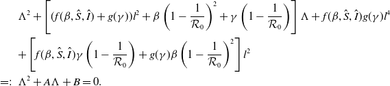 \begin{eqnarray} &&\Lambda ^2+\left [(f(\beta ,\hat {S},\hat {I})+g(\gamma ))l^2+\beta \left (1-\frac {1}{\mathcal{R}_0}\right )^2+\gamma \left (1-\frac {1}{\mathcal{R}_0}\right )\right ]\Lambda +f(\beta ,\hat {S},\hat {I})g(\gamma )l^4\nonumber \\ &&+\left [f(\beta ,\hat {S},\hat {I})\gamma \left (1-\frac {1}{\mathcal{R}_0}\right )+g(\gamma )\beta \left (1-\frac {1}{\mathcal{R}_0}\right )^2\right ]l^2\nonumber \\ &\,=\!:\,&\Lambda ^2+A\Lambda +B=0. \end{eqnarray}
It is easily seen that constants $A$
and
$A$
and $B$
are positive since
$B$
are positive since $\mathcal{R}_0\gt 1$
. Let
$\mathcal{R}_0\gt 1$
. Let $\Lambda _1$
and
$\Lambda _1$
and $\Lambda _2$
denote the two eigenvalues of (4.3). Thus,
$\Lambda _2$
denote the two eigenvalues of (4.3). Thus, $\Lambda _1+\Lambda _2=-A\lt 0$
and
$\Lambda _1+\Lambda _2=-A\lt 0$
and $\Lambda _1\Lambda _2=B\gt 0$
, indicating the real parts of the eigenvalues are negative. This proves the local stability of the EE.
$\Lambda _1\Lambda _2=B\gt 0$
, indicating the real parts of the eigenvalues are negative. This proves the local stability of the EE.
The disease is always extinct if the basic reproduction number is less than one in the following sense.
Lemma 4.2.
If $\mathcal{R}_0$
(1.5)
$\mathcal{R}_0$
(1.5) $\lt 1$
or
$\lt 1$
or $\mathcal{R}_0$
(1.6)
$\mathcal{R}_0$
(1.6) $\lt 1$
, then
$\lt 1$
, then $I(x,t)\rightarrow 0$
exponentially as
$I(x,t)\rightarrow 0$
exponentially as $t\rightarrow \infty$
.
$t\rightarrow \infty$
.
Proof. The proof is standard via the comparison principle for parabolic equations as in [Reference Allen, Bolker, Lou and Nevai1, Lemma 2.5].
4.1. Threshold dynamics for Fickian diffusion
We now establish the threshold dynamics in terms of $\mathcal{R}_0$
(1.5) for (1.5).
$\mathcal{R}_0$
(1.5) for (1.5).
Proposition 4.2. Assume that (H1)–(H4) hold. The following assertions hold.
(i) If $\mathcal{R}_0$
(1.5)
$\mathcal{R}_0$
(1.5) $\leq 1$
, then the solution
$\leq 1$
, then the solution $(S,I)$
of (
1.5
) satisfies
$(S,I)$
of (
1.5
) satisfies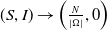 $(S,I)\rightarrow \left (\frac {N}{|\Omega |},0\right )$
as
$(S,I)\rightarrow \left (\frac {N}{|\Omega |},0\right )$
as $t\rightarrow \infty$
.
$t\rightarrow \infty$
.
(ii) If $\mathcal{R}_0$
(1.5)
$\mathcal{R}_0$
(1.5) $\gt 1$
, then (
1.5
) is uniformly persistent, i.e., there exists some constant
$\gt 1$
, then (
1.5
) is uniformly persistent, i.e., there exists some constant $\rho \gt 0$
such that
$\rho \gt 0$
such that
 \begin{equation*}\liminf _{t\rightarrow \infty }S(x,t)\geq \rho \ \mathrm {and}\ \liminf _{t\rightarrow \infty }I(x,t)\geq \rho \ \mathrm {uniformly for}\ x\in \bar {\Omega }.\end{equation*}
Moreover, there exists at least one EE for ( 1.5 ).
Proof. (i) can be proved similarly as [Reference Cui, Lam and Lou10, Theorem 1.1(a)] for $\mathcal{R}_0$
(1.5)
$\mathcal{R}_0$
(1.5) $\leq 1$
. According to Theorem2.1, we conclude that the solution of (1.5) is ultimately bounded for large time. Then, by the dynamical system theory developed in [Reference Zhao32], we can adapt [Reference Wang, Wang and Kim29] to verify the uniform persistence and the existence of EE for (1.5) with
$\leq 1$
. According to Theorem2.1, we conclude that the solution of (1.5) is ultimately bounded for large time. Then, by the dynamical system theory developed in [Reference Zhao32], we can adapt [Reference Wang, Wang and Kim29] to verify the uniform persistence and the existence of EE for (1.5) with $\mathcal{R}_0$
(1.5)
$\mathcal{R}_0$
(1.5) $\gt 1$
. Proposition4.2 thus follows.
$\gt 1$
. Proposition4.2 thus follows.
We then show the global stability of the constant EE when $\beta/\gamma$
is a positive constant on
$\beta/\gamma$
is a positive constant on $\Omega$
via the Lyapunov functional method.
$\Omega$
via the Lyapunov functional method.
Theorem 4.1.
Suppose that $\beta /\gamma$
is constant on
$\beta /\gamma$
is constant on $\Omega$
. If
$\Omega$
. If $\mathcal{R}_0\gt 1$
, then the constant EE of (
1.5
) is globally asymptotically stable.
$\mathcal{R}_0\gt 1$
, then the constant EE of (
1.5
) is globally asymptotically stable.
Proof. Let
 \begin{equation*}V(S,I)=\int \frac {S^2-\hat {S}^2}{S^2}dS+\int \frac {I^2-\hat {I}^2}{I^2}dI.\end{equation*}
We construct a Lyapunov functional to verify the global attractiveness of the constant EE as follows:
 \begin{equation*} L_1(t)=\int _\Omega V(S(x,t),I(x,t))dx. \end{equation*}
Computing the total differential of $L_1(t)$
leads to
$L_1(t)$
leads to
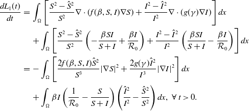 \begin{eqnarray*} \frac {dL_1(t)}{dt}&=&\int _\Omega \left [\frac {S^2-\hat {S}^2}{S^2}\nabla \cdot (f(\beta ,S,I)\nabla S)+\frac {I^2-\hat {I}^2}{I^2}\nabla \cdot (g(\gamma )\nabla I)\right ]dx\\ &&+\int _\Omega \left [\frac {S^2-\hat {S}^2}{S^2}\left ({-}\frac {\beta SI}{S+I}+\frac {\beta I}{\mathcal{R}_0}\right )+\frac {I^2-\hat {I}^2}{I^2}\left (\frac {\beta SI}{S+I}-\frac {\beta I}{\mathcal{R}_0}\right )\right ]dx\\ &=&-\int _\Omega \left [\frac {2f(\beta ,S,I)\hat {S}^2}{S^3}|\nabla S|^2+\frac {2g(\gamma )\hat {I}^2}{I^3}|\nabla I|^2\right ]dx\\ &&+\int _\Omega \beta I\left (\frac {1}{\mathcal{R}_0}-\frac {S}{S+I}\right )\left (\frac {\hat {I}^2}{I^2}-\frac {\hat {S}^2}{S^2}\right )dx,\ \forall \ t\gt 0. \end{eqnarray*}
Since $\frac {\hat {S}}{\hat {S}+\hat {I}}=\frac {1}{\mathcal{R}_0}$
and
$\frac {\hat {S}}{\hat {S}+\hat {I}}=\frac {1}{\mathcal{R}_0}$
and $f(\beta ,S,I),\ g(\gamma )\gt 0$
, we have
$f(\beta ,S,I),\ g(\gamma )\gt 0$
, we have
 \begin{eqnarray*} \frac {dL_1(t)}{dt}&=&-\int _\Omega \left [\frac {2f(\beta ,S,I)\hat {S}^2}{S^3}|\nabla S|^2+\frac {2g(\gamma )\hat {I}^2}{I^3}|\nabla I|^2\right ]dx\\ &&-\int _\Omega \frac {\beta S\hat {I}^2}{(S+I)(\hat {S}+\hat {I})}\left (\frac {\hat {S}}{S}+\frac {\hat {I}}{I}\right )\left (\frac {\hat {S}}{S}-\frac {\hat {I}}{I}\right )^2dx\leq 0,\ \forall \ t\gt 0. \end{eqnarray*}
The equality holds only at $(\hat {S},\hat {I})$
. Therefore,
$(\hat {S},\hat {I})$
. Therefore, $L_1(t)$
is a Lyapunov functional for (1.5). It then follows from some standard arguments that
$L_1(t)$
is a Lyapunov functional for (1.5). It then follows from some standard arguments that
 \begin{equation*}(S(\cdot ,t),I(\cdot ,t))\rightarrow (\hat {S},\hat {I})\ \textrm {in}\ (L^2(\Omega ))^2,\ \textrm {as}\ t\rightarrow \infty .\end{equation*}
By Theorem2.1, we have $\|S(\cdot ,t)\|_{L^\infty (\Omega )}$
and
$\|S(\cdot ,t)\|_{L^\infty (\Omega )}$
and $\|I(\cdot ,t)\|_{L^\infty (\Omega )}$
are bounded for all
$\|I(\cdot ,t)\|_{L^\infty (\Omega )}$
are bounded for all $t\geq 0$
. Thus, we obtain
$t\geq 0$
. Thus, we obtain
 \begin{equation*}(S(\cdot ,t),I(\cdot ,t))\rightarrow (\hat {S},\hat {I})\ \textrm {in}\ (L^\infty (\Omega ))^2,\ \textrm {as}\ t\rightarrow \infty .\end{equation*}
This indicates the global attractiveness of the constant EE of (1.5). According to the local stability stated in Lemma4.1, we deduce that the constant EE of (1.5) is globally asymptotically stable.
4.2. Threshold dynamics for the Fokker–Planck-type diffusion
Throughout this subsection, we assume that $\beta$
and
$\beta$
and $\gamma$
are constants on
$\gamma$
are constants on $\Omega$
. We first prove the global stability of the DFE for (1.6) if
$\Omega$
. We first prove the global stability of the DFE for (1.6) if $\mathcal{R}_0\leq 1$
through energy estimates. Let
$\mathcal{R}_0\leq 1$
through energy estimates. Let $U(x,t)=S(x,t)+I(x,t)$
for
$U(x,t)=S(x,t)+I(x,t)$
for $x\in \bar {\Omega }$
and
$x\in \bar {\Omega }$
and $t\geq 0$
. If
$t\geq 0$
. If $\beta$
and
$\beta$
and $\gamma$
are constant on
$\gamma$
are constant on $\Omega$
, then (1.6) degenerates to
$\Omega$
, then (1.6) degenerates to
 \begin{equation} \left \{\begin{aligned} &\partial _t U=\nabla \cdot [(f+f_S S)\nabla U]+\nabla \cdot [(g-f+(f_I-f_S)S)\nabla I],\ &x&\in \Omega ,\ t\gt 0,\\ &\nabla U\cdot \mathbf{n}=0,\ &x&\in \partial \Omega ,\ t\gt 0,\\ &U(x,0)=S_0(x)+I_0(x),\ &x&\in \Omega . \end{aligned}\right . \end{equation}
In view of Theorem2.2, there exists a positive constant $K$
such that
$K$
such that $f_S,f_I\leq K$
for all
$f_S,f_I\leq K$
for all $t\gt 0$
.
$t\gt 0$
.
Lemma 4.3.
Assume that (H1)–(H4) hold and $\beta$
and
$\beta$
and $\gamma$
are constant on
$\gamma$
are constant on $\Omega$
. The solution
$\Omega$
. The solution $U$
of (
4.4
) fulfils that
$U$
of (
4.4
) fulfils that
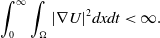 \begin{equation} \int _0^{\infty }\int _\Omega |\nabla U|^2dxdt\lt \infty . \end{equation}
Proof. We multiply the second equation of (1.6) by $I$
and integrate over
$I$
and integrate over $\Omega \times (0,T)$
to result in
$\Omega \times (0,T)$
to result in
 \begin{eqnarray} g(\gamma )\int _0^T\int _\Omega |\nabla I|^2dx&=&\frac {1}{2}\int _\Omega I_0^2dx-\frac {1}{2}\int _\Omega I^2(\cdot ,T)dx+\int _0^T\int _\Omega \left (\frac {\beta S}{S+I}-\gamma\right )I^2dxdt\nonumber \\[4pt] &\leq &\frac {1}{2}\int _\Omega I_0^2dx+\beta \int _0^T\int _\Omega I^2dxdt. \end{eqnarray}
Since $\beta$
and
$\beta$
and $\gamma$
are constant on
$\gamma$
are constant on $\Omega$
. It follows from [Reference Allen, Bolker, Lou and Nevai1, Lemma 2.3(d)] that
$\Omega$
. It follows from [Reference Allen, Bolker, Lou and Nevai1, Lemma 2.3(d)] that $\mu ^*=\nu ^*\gt 0$
as
$\mu ^*=\nu ^*\gt 0$
as $\mathcal{R}_0\lt 1$
. Since
$\mathcal{R}_0\lt 1$
. Since $\partial _tI\leq g(\gamma )\Delta I+(\beta -\gamma )I$
for
$\partial _tI\leq g(\gamma )\Delta I+(\beta -\gamma )I$
for $x\in \Omega$
and
$x\in \Omega$
and $t\gt 0$
, it can be shown that
$t\gt 0$
, it can be shown that $Me^{-\nu ^*t}\phi ^*(x)$
is a super-solution to the
$Me^{-\nu ^*t}\phi ^*(x)$
is a super-solution to the $I$
-equation for a large enough constant
$I$
-equation for a large enough constant $M\gt 0$
. By comparison principle, one has
$M\gt 0$
. By comparison principle, one has
 \begin{equation} I(x,t)\leq Me^{-\nu ^*t}\phi ^*(x),\ x\in \Omega ,\ t\gt 0. \end{equation}
We substitute (4.7) to (4.6) to yield
 \begin{equation} \int _0^T\int _\Omega |\nabla I|^2dx\leq C\left [\int _\Omega I_0^2dx+\int _0^T\int _\Omega (M e^{-\nu ^*t}\phi ^*(x))^2dxdt\right ]\leq C,\ \forall \ T\gt 0, \end{equation}
for positive constant $C$
independent of
$C$
independent of $T$
. We then multiply the first equation of (1.6) by
$T$
. We then multiply the first equation of (1.6) by $S$
and integrate by parts over
$S$
and integrate by parts over $\Omega$
to get
$\Omega$
to get
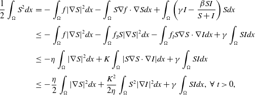 \begin{eqnarray*} \frac {1}{2}\int _\Omega S^2dx&=&-\int _\Omega f|\nabla S|^2dx-\int _\Omega S\nabla f\cdot \nabla Sdx+\int _\Omega \left (\gamma I-\frac {\beta SI}{S+I}\right )Sdx\\[3pt] &\leq &-\int _\Omega f|\nabla S|^2dx-\int _\Omega f_S S|\nabla S|^2dx-\int _\Omega f_IS\nabla S\cdot \nabla Idx+\gamma \int _\Omega SIdx\\[3pt] &\leq &-\eta \int _\Omega |\nabla S|^2dx+K\int _\Omega |S\nabla S\cdot \nabla I|dx+\gamma \int _\Omega SIdx\\[3pt] &\leq &-\frac {\eta }{2}\int _\Omega |\nabla S|^2dx+\frac {K^2}{2\eta }\int _\Omega S^2|\nabla I|^2dx+\gamma \int _\Omega SIdx,\ \forall \ t\gt 0, \end{eqnarray*}
where $K$
is given in the proof of Lemma2.4 and Young’s inequality is used in the last inequality. Since
$K$
is given in the proof of Lemma2.4 and Young’s inequality is used in the last inequality. Since $S$
is bounded by Theorem2.2 for all
$S$
is bounded by Theorem2.2 for all $t\gt 0$
, one has
$t\gt 0$
, one has
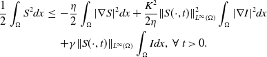 \begin{eqnarray} \frac {1}{2}\int _\Omega S^2dx&\leq &-\frac {\eta }{2}\int _\Omega |\nabla S|^2dx+\frac {K^2}{2\eta }\|S(\cdot ,t)\|_{L^\infty (\Omega )}^2\int _\Omega |\nabla I|^2dx\nonumber \\ &&+\gamma \|S(\cdot ,t)\|_{L^\infty (\Omega )}\int _\Omega Idx,\ \forall \ t\gt 0. \end{eqnarray}
We integrate both sides of (4.9) from 0 to $T$
to give
$T$
to give
 \begin{eqnarray} \int _0^T\int _\Omega |\nabla S|^2dxdt&\leq & C\left [\int _\Omega S_0^2dx+\int _0^T\int _\Omega |\nabla I|^2dxdt+\int _0^T\int _\Omega M e^{-\mu ^*t}\phi ^*(x)dxdt\right ]\nonumber \\ &\leq & C,\ \forall \ T\gt 0. \end{eqnarray}
Since $C$
is independent of
$C$
is independent of $T$
, consequently, we combine (4.8) and (4.10) to produce (4.5).
$T$
, consequently, we combine (4.8) and (4.10) to produce (4.5).
We then show that $U_t$
decays at least in the dual space of
$U_t$
decays at least in the dual space of $H^1(\Omega )$
.
$H^1(\Omega )$
.
Lemma 4.4.
Assume that (H1)–(H4) hold and $\beta$
and
$\beta$
and $\gamma$
are constant on
$\gamma$
are constant on $\Omega$
. The solution
$\Omega$
. The solution $U$
of (
4.4
) satisfies
$U$
of (
4.4
) satisfies
 \begin{equation*} \int _0^\infty \|U_t(\cdot ,t)\|_{(H^1(\Omega ))^*}^2dt\lt \infty , \end{equation*}
where $(H^1(\Omega ))^*$
represents the dual space of
$(H^1(\Omega ))^*$
represents the dual space of $H^1(\Omega )$
.
$H^1(\Omega )$
.
Proof. By virtue of the forms of $f$
, we can infer that
$f$
, we can infer that $f\leq K_0$
for some positive constant
$f\leq K_0$
for some positive constant $K_0\,:\!=\,K_0(\beta ,k,\eta ,\|S(\cdot ,t)\|_{L^\infty (\Omega )})$
if
$K_0\,:\!=\,K_0(\beta ,k,\eta ,\|S(\cdot ,t)\|_{L^\infty (\Omega )})$
if $\|S(\cdot ,t)\|_{L^\infty (\Omega )}$
is bounded for all
$\|S(\cdot ,t)\|_{L^\infty (\Omega )}$
is bounded for all $t\geq 0$
. We multiply both sides of the first equation of (4.4) by any test function
$t\geq 0$
. We multiply both sides of the first equation of (4.4) by any test function $\theta \in H^1(\Omega )$
and integrate by parts over
$\theta \in H^1(\Omega )$
and integrate by parts over $\Omega$
to produce
$\Omega$
to produce
 \begin{eqnarray*} \int _\Omega \theta \partial _tUdx&=&-\int _\Omega [(f+f_S S)\nabla U]\cdot \nabla \theta dx-\int _\Omega [(g-f+(f_I-f_S)S)\nabla I]\cdot \nabla \theta dx\\ &\leq &(K_0+K\|S(\cdot ,t)\|_{L^\infty (\Omega )})\int _\Omega |\nabla U\cdot \nabla \theta |dx\\ &&+(g+K_0+2K\|S(\cdot ,t)\|_{L^\infty (\Omega )})\int _\Omega |\nabla I\cdot \nabla \theta |dx\\ &\leq &C\left (\|\nabla U(\cdot ,t)\|_{L^2(\Omega )}\|\nabla \theta \|_{L^2(\Omega )}+\|\nabla I(\cdot ,t)\|_{L^2(\Omega )}\|\nabla \theta \|_{L^2(\Omega )}\right )\\ &\leq &C\left (\|\nabla U(\cdot ,t)\|_{L^2(\Omega )}+\|\nabla I(\cdot ,t)\|_{L^2(\Omega )}\right )\|\nabla \theta \|_{H^1(\Omega )},\ \forall \ t\gt 0, \end{eqnarray*}
for some positive constant $C$
. Hence,
$C$
. Hence, $U_t(\cdot ,t)\in (H^1(\Omega ))^*$
and satisfies
$U_t(\cdot ,t)\in (H^1(\Omega ))^*$
and satisfies
 \begin{eqnarray*} \|U_t(\cdot ,t)\|_{(H^1(\Omega ))^*}\leq C\left (\|\nabla U(\cdot ,t)\|_{L^2(\Omega )}+\|\nabla I(\cdot ,t)\|_{L^2(\Omega )}\right ),\ \forall \ t\gt 0. \end{eqnarray*}
In light of (4.5) and (4.8), we conclude
 \begin{equation*} \int _0^\infty \|U_t(\cdot ,t)\|^2_{(H^1(\Omega ))^*}dt\leq C\int _0^\infty \left (\|\nabla U(\cdot ,t)\|_{L^2(\Omega )}^2+\|\nabla I(\cdot ,t)\|_{L^2(\Omega )}^2\right )dt\lt \infty . \end{equation*}
Now we are able to demonstrate the stability of the DFE for (1.6) with $\mathcal{R}_0\leq 1$
.
$\mathcal{R}_0\leq 1$
.
Theorem 4.2.
Assume that (H1)–(H4) hold and $\beta$
and
$\beta$
and $\gamma$
are constant on
$\gamma$
are constant on $\Omega$
. If
$\Omega$
. If $\mathcal{R}_0\leq 1$
, the the solution of (
1.6
) satisfies
$\mathcal{R}_0\leq 1$
, the the solution of (
1.6
) satisfies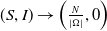 $(S,I)\rightarrow \left (\frac {N}{|\Omega |},0\right )$
in
$(S,I)\rightarrow \left (\frac {N}{|\Omega |},0\right )$
in $C(\bar {\Omega })$
as
$C(\bar {\Omega })$
as $t\rightarrow \infty$
.
$t\rightarrow \infty$
.
Proof. We first consider $\mathcal{R}_0\lt 1$
. By Lemma4.2, we know
$\mathcal{R}_0\lt 1$
. By Lemma4.2, we know $I(x,t)\rightarrow 0$
exponentially for
$I(x,t)\rightarrow 0$
exponentially for $x\in \bar {\Omega }$
as
$x\in \bar {\Omega }$
as $t\rightarrow \infty$
. We proceed with a similar argument as [Reference Li, Peng and Xiang17, Theorem 3.5] to deduce that
$t\rightarrow \infty$
. We proceed with a similar argument as [Reference Li, Peng and Xiang17, Theorem 3.5] to deduce that
 \begin{equation*} \left \|U(\cdot ,t)-\frac {N}{|\Omega |}\right \|_{C(\bar {\Omega })}\rightarrow 0,\ \mathrm {as}\ t\rightarrow \infty . \end{equation*}
This indicates that $S(x,t)\rightarrow \frac {N}{|\Omega |}$
in
$S(x,t)\rightarrow \frac {N}{|\Omega |}$
in $C(\bar {\Omega })$
as
$C(\bar {\Omega })$
as $t\rightarrow \infty$
.
$t\rightarrow \infty$
.
We then consider the case $\mathcal{R}_0=1$
. This is equivalent to
$\mathcal{R}_0=1$
. This is equivalent to $\beta =\gamma$
. The second equation of (1.6) becomes
$\beta =\gamma$
. The second equation of (1.6) becomes
 \begin{equation} \partial _t I=g\Delta I-\frac {\beta I^2}{S+I}\leq g\Delta I-\frac {\beta }{M_5}I^2,\ x\in \bar {\Omega },\ t\gt 0, \end{equation}
where we use the bound of $S+I$
by Theorem2.2. We turn to the following Cauchy problem
$S+I$
by Theorem2.2. We turn to the following Cauchy problem
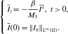 \begin{equation*} \left \{\begin{aligned} &\bar {I}_t=-\frac {\beta }{M_5}\bar {I}^2,\ t\gt 0,\\[2pt] &\bar {I}(0)=\|I_0\|_{L^\infty (\Omega )}. \end{aligned}\right . \end{equation*}
It can be verified that $\bar {I}$
is a super-solution of (4.11). It follows from the comparison principle that
$\bar {I}$
is a super-solution of (4.11). It follows from the comparison principle that
 \begin{equation} I(\cdot ,t)\leq \bar {I}(t)=\left (\frac {1}{\bar {I_0}}+\frac {\beta t}{M_5}\right )^{-1}\rightarrow 0,\ \textrm {as}\ t\rightarrow \infty . \end{equation}
We then multiply the first equation of (1.6) by $S$
and integrate by parts over
$S$
and integrate by parts over $\Omega$
to yield
$\Omega$
to yield
 \begin{eqnarray*} \frac {1}{2}\frac {d}{dt}\int _\Omega S^2dx&=&-\int _\Omega f|\nabla S|^2dx-\int _\Omega S\nabla f\cdot \nabla Sdx+\beta \int _\Omega \frac {SI^2}{S+I}dx\\ &\leq &-\frac {\eta }{2}\int _\Omega |\nabla S|^2dx+\frac {K^2}{2\eta }\|S(\cdot ,t)\|_{L^\infty (\Omega )}^2\int _\Omega |\nabla I|^2dx+\beta \int _\Omega I^2dx,\ \forall \ t\gt 0. \end{eqnarray*}
As a result of (4.12) and Theorem2.2, we conclude that
 \begin{equation*} \int _0^\infty \int _\Omega |\nabla S|^2dxdt\lt \infty ,\ \forall \ T\gt 0 \end{equation*}
also holds for $\mathcal{R}_0=1$
. We then follow similar arguments as those in
$\mathcal{R}_0=1$
. We then follow similar arguments as those in $\mathcal{R}_0\lt 1$
. This completes the proof.
$\mathcal{R}_0\lt 1$
. This completes the proof.
We now dedicate to the stability of the constant EE. By the standard Moser-type iteration, we can get the following boundedness for $I$
of (1.6).
$I$
of (1.6).
Lemma 4.5.
Assume that (H1)–(H4) hold. There exists a positive constant $M_6$
independent of
$M_6$
independent of $\eta$
and
$\eta$
and $K$
such that
$K$
such that
 \begin{equation} \|I(\cdot ,t)\|_{L^\infty (\Omega )}\leq M_6,\ \forall \ t\gt 0. \end{equation}
To give the global stability of the constant EE for (1.6), we construct another Lyapunov functional.
Theorem 4.3.
Assume that (H1)–(H4) hold and $\beta$
and
$\beta$
and $\gamma$
are constant on
$\gamma$
are constant on $\Omega$
. If
$\Omega$
. If $\mathcal{R}_0\gt 1+\frac {M_6^2 K^2}{4g \eta }$
, then the constant EE of (
1.6
) is globally asymptotically stable.
$\mathcal{R}_0\gt 1+\frac {M_6^2 K^2}{4g \eta }$
, then the constant EE of (
1.6
) is globally asymptotically stable.
Proof. We employ the following Lyapunov functional
 \begin{equation*}L_2(t)=\int _\Omega \left [\left (S- \hat {S}-\hat {S}\ln \frac {\hat {S}}{S}\right )+\left (I- \hat {I}-\hat {I}\ln \frac {\hat {I}}{I}\right )\right ]dx.\end{equation*}
We integrate by parts to compute the total derivatives of $L_2(t)$
to give
$L_2(t)$
to give
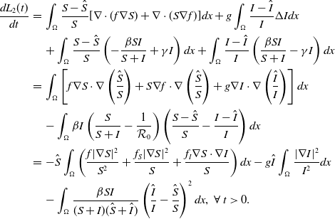 \begin{eqnarray} \frac {dL_2(t)}{dt}&=&\int _\Omega \frac {S-\hat {S}}{S}[\nabla \cdot (f\nabla S)+\nabla \cdot (S\nabla f)]dx+g\int _\Omega \frac {I-\hat {I}}{I}\Delta Idx\nonumber \\ &&+\int _\Omega \frac {S-\hat {S}}{S}\left ({-}\frac {\beta SI}{S+I}+\gamma I\right )dx+\int _\Omega \frac {I-\hat {I}}{I}\left (\frac {\beta SI}{S+I}-\gamma I\right )dx\nonumber \\ &=&\int _\Omega \left [f\nabla S\cdot \nabla \left (\frac {\hat {S}}{S}\right )+S\nabla f\cdot \nabla \left (\frac {\hat {S}}{S}\right )+g\nabla I\cdot \nabla \left (\frac {\hat {I}}{I}\right )\right ]dx\nonumber \\ &&-\int _\Omega \beta I\left (\frac {S}{S+I}-\frac {1}{\mathcal{R}_0}\right )\left (\frac {S-\hat {S}}{S}-\frac {I-\hat {I}}{I}\right )dx\nonumber \\ &=&-\hat {S}\int _\Omega \left (\frac {f|\nabla S|^2}{S^2}+\frac {f_S|\nabla S|^2}{S}+\frac {f_I\nabla S\cdot \nabla I}{S}\right )dx-g\hat {I}\int _\Omega \frac {|\nabla I|^2}{I^2}dx\nonumber \\ &&-\int _\Omega \frac {\beta SI}{(S+I)(\hat {S}+\hat {I})}\left (\frac {\hat {I}}{I}-\frac {\hat {S}}{S}\right )^2dx,\ \forall \ t\gt 0. \end{eqnarray}
Since $f_S\geq 0$
, we drop the second term on the right-hand side of (4.14). By assumption (H2) and
$f_S\geq 0$
, we drop the second term on the right-hand side of (4.14). By assumption (H2) and $\hat {I}=(\mathcal{R}_0-1)\hat {S}$
, we have
$\hat {I}=(\mathcal{R}_0-1)\hat {S}$
, we have
 \begin{eqnarray*} \frac {dL_2(t)}{dt}&\leq &-\eta \hat {S}\int _\Omega \frac {|\nabla S|^2}{S^2}dx-g\hat {I}\int _\Omega \frac {|\nabla I|^2}{I^2}dx+K\hat {S}\int _\Omega \frac {|\nabla S||\nabla I|}{S}dx\\[4pt] &&-\frac {\beta \hat {S}}{\mathcal{R}_0}\int _\Omega \frac {[(\mathcal{R}_0-1)S-I]^2}{(S+I)S}dx\\[4pt] &\leq &-\hat {S}\int _\Omega \left (\frac {\sqrt {\eta }|\nabla S|}{S}-\frac {K|\nabla I|}{2\sqrt {\eta }}\right )^2dx-\hat {S}\int _\Omega \left ((\mathcal{R}_0-1)g-\frac {I^2K^2}{4\eta }\right )\frac {|\nabla I|^2}{I^2}dx\\[4pt] &&-\frac {\beta \hat {S}}{\mathcal{R}_0}\int _\Omega \frac {[(\mathcal{R}_0-1)S-I]^2}{(S+I)S}dx,\ \forall \ t\gt 0. \end{eqnarray*}
Since $\mathcal{R}_0\gt 1+\frac {M_6^2 K^2}{4g \eta }$
, by (4.13), one can find a positive constant
$\mathcal{R}_0\gt 1+\frac {M_6^2 K^2}{4g \eta }$
, by (4.13), one can find a positive constant $C$
such that
$C$
such that
 \begin{equation*} \frac {dL_2(t)}{dt}\leq -C\int _\Omega \left [|\nabla S|^2+|\nabla I|^2+((\mathcal{R}_0-1)S-I)^2\right ]dx. \end{equation*}
It then follows from the argument in [Reference Li, Peng and Xiang17, Theorem 3.6(i)] that
 \begin{equation*}(S(\cdot ,t),I(\cdot ,t))\rightarrow (\hat {S},\hat {I})\ \textrm {in}\ (L^\infty (\Omega ))^2,\ \textrm {as}\ t\rightarrow \infty .\end{equation*}
This completes the proof.
4.3. Numerical examples
We now present numerical examples to validate the theoretical results of the threshold dynamics. We choose $k=\eta =0.1$
and
$k=\eta =0.1$
and $S_0=I_0=50$
. Simulation results for (1.5) and (1.6) are displayed in Figure 1 in terms of the basic reproduction number
$S_0=I_0=50$
. Simulation results for (1.5) and (1.6) are displayed in Figure 1 in terms of the basic reproduction number $\mathcal{R}_0$
. In Figure 1(a) and (d), the disease is extinct as
$\mathcal{R}_0$
. In Figure 1(a) and (d), the disease is extinct as $\mathcal{R}_0=\frac {1}{3}\lt 1$
. A similar extinction tendency is also observed in Figure 1(b) and (e) as
$\mathcal{R}_0=\frac {1}{3}\lt 1$
. A similar extinction tendency is also observed in Figure 1(b) and (e) as $\mathcal{R}_0=1$
. The disease is persistent in Figure 1(c) and (f) as
$\mathcal{R}_0=1$
. The disease is persistent in Figure 1(c) and (f) as $\mathcal{R}_0=3\gt 1$
.
$\mathcal{R}_0=3\gt 1$
.


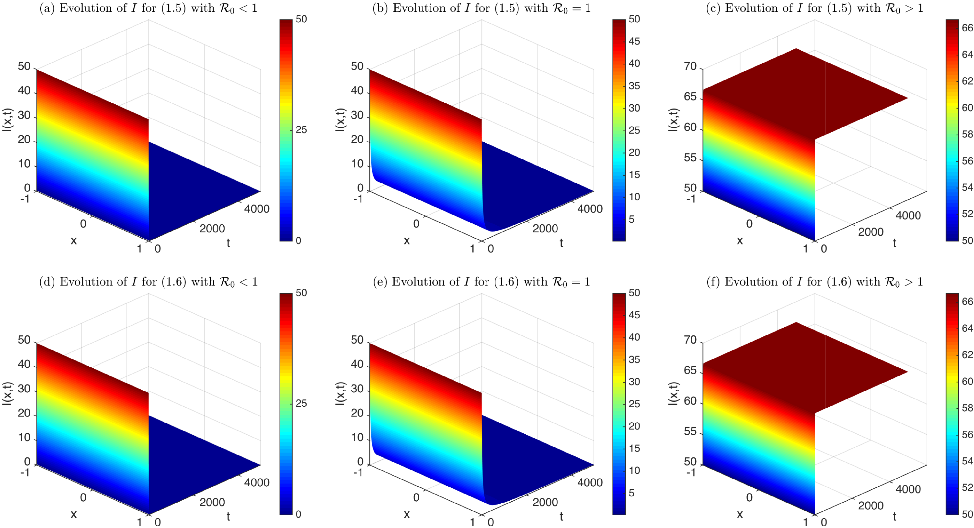
5. Spatial segregation
Spatial segregation is a phenomenon where population groups are separated spontaneously in certain areas [Reference Schelling24]. In [Reference Mimura and Kawasaki22], Mimura and Kawasaki discussed spatial segregation in a competitive interaction-diffusion system. A series of works have been done on this topic in epidemic modelling with cognitive diffusion, see recent publications [Reference Liu, Wang and Zhang18, Reference Wang, Wang and Kim29]. This section aims to explore the effect of diffusion rates on spatial segregation by comparing it with the numerical results in [Reference Wang, Wang and Kim29]. We apply the segregation indices introduced in [Reference Wang, Wang and Kim29] to measure the degree of segregation:
 \begin{equation*} \kappa (u_1,u_2)=\frac {\|u_1-u_2\|_{L^1(\Omega )}}{\|u_1\|_{L^1(\Omega )}+\|u_2\|_{L^1(\Omega )}}, \end{equation*}
and
 \begin{equation*} \chi (u_1,u_2)=\max _{x\in \bar {\Omega }}\{u_1-u_2\}\cdot \min _{x\in \bar {\Omega }}\{u_1-u_2\}, \end{equation*}
for $u_i(x)\in C(\bar {\Omega })$
. Spatial segregation of two populations
$u_i(x)\in C(\bar {\Omega })$
. Spatial segregation of two populations $u_1$
and
$u_1$
and $u_2$
can be described in the following way: For
$u_2$
can be described in the following way: For $\chi (u_1,u_2)\lt 0$
, the segregation is strong or perfect if
$\chi (u_1,u_2)\lt 0$
, the segregation is strong or perfect if $\kappa (u_1,u_2)$
is close to 1, while it is weak or poor if
$\kappa (u_1,u_2)$
is close to 1, while it is weak or poor if $\kappa (u_1,u_2)$
is close to 0. Whereas, the segregation phenomenon disappears if
$\kappa (u_1,u_2)$
is close to 0. Whereas, the segregation phenomenon disappears if $\kappa (u_1,u_2)=0$
or
$\kappa (u_1,u_2)=0$
or $\chi (u_1,u_2)\geq 0$
.
$\chi (u_1,u_2)\geq 0$
.
In the following numerical examples, we consider two types of dispersal strategies for infected individuals. If infectives’ movement is determined by the recovery rate, the diffusion rate is $g(\gamma )$
. This pattern is analysed theoretically in Sections 2–4.
$g(\gamma )$
. This pattern is analysed theoretically in Sections 2–4.
The infection-recovery rates. (a) $\beta =6\cos x+6.6$
,
$\beta =6\cos x+6.6$
, $\gamma =\cos x+1.5$
; (b)
$\gamma =\cos x+1.5$
; (b) $\beta =6\cos x+6.6$
,
$\beta =6\cos x+6.6$
, $\gamma =\sin x+1.5$
; (c)
$\gamma =\sin x+1.5$
; (c) $\beta =5e^{-160(x-0.2)^2}+4$
,
$\beta =5e^{-160(x-0.2)^2}+4$
, $\gamma =5e^{-160(x-0.8)^2}+2$
.
$\gamma =5e^{-160(x-0.8)^2}+2$
.
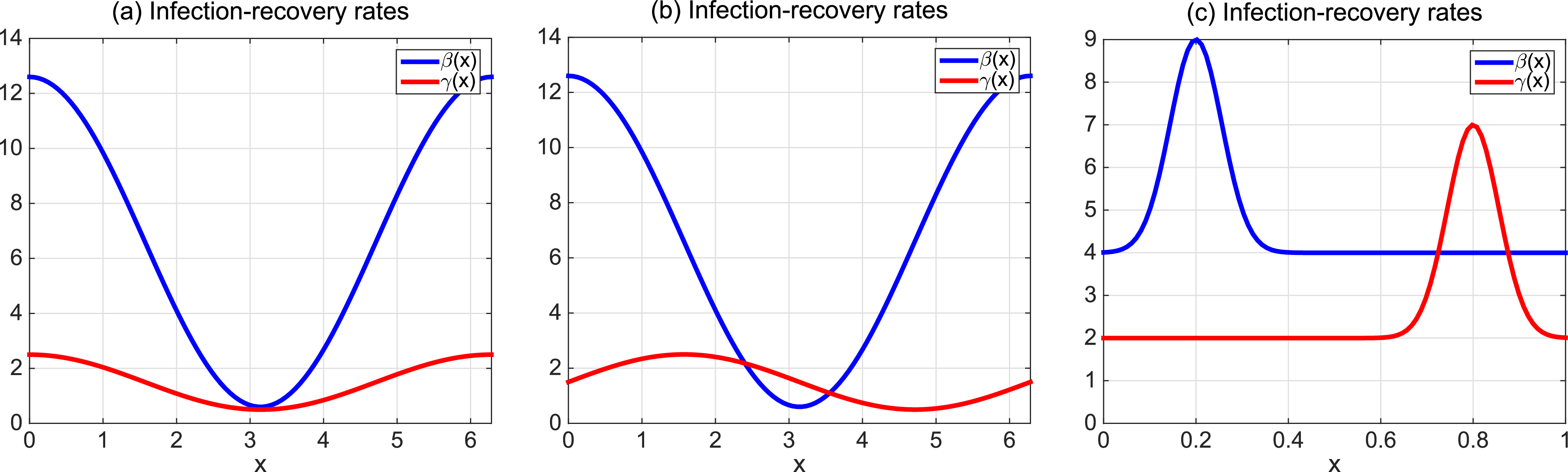
To elucidate the dynamics of quasilinear systems (1.5) and (1.6), we draw comparisons with the semilinear systems (1.3) and (1.4). In [Reference Wang, Wang and Kim29], various forms of infection and recovery rates, leading to diverse diffusion rate formulations, have been explored. We consider three types of dependence for the diffusion rates, including linear dependence, exponential dependence and algebraic dependence. In the following examples, we take $\Omega$
as an open interval and the initial data
$\Omega$
as an open interval and the initial data $S_0(x)=I_0(x)=500$
. The infection and recovery rates we take are shown in Figure 2.
$S_0(x)=I_0(x)=500$
. The infection and recovery rates we take are shown in Figure 2.
5.1. Linear dependence
In this subsection, we study the epidemic dynamics in the cases where the dispersal rates are in the linear form, and the infection and recovery rates are taken as Figure 2(a). The simulation for semilinear systems (1.3) and (1.4) is displayed in Figure 3(a) and (d). For Fickian law of diffusion, system (1.5) becomes:
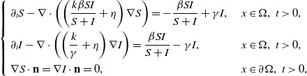 \begin{equation} \left \{\begin{aligned} &\partial _t S-\nabla \cdot \left (\left (\frac {k\beta SI}{S+I}+\eta \right )\nabla S \right )=-\frac {\beta SI}{S+I}+\gamma I,\ & x&\in \Omega ,\ t\gt 0,\\ &\partial _t I-\nabla \cdot \left (\left (\frac {k}{\gamma }+\eta \right )\nabla I\right )=\frac {\beta SI}{S+I}-\gamma I,\ & x&\in \Omega ,\ t\gt 0,\\ &\displaystyle \nabla S\cdot \mathbf{n}=\nabla I\cdot \mathbf{n}=0,\ & x&\in \partial \Omega ,\ t\gt 0, \end{aligned}\right . \end{equation}
and the steady state of (5.1) is shown in Figure 3(b). For the Fokker–Planck-type law of diffusion, system (1.6) can be written as:
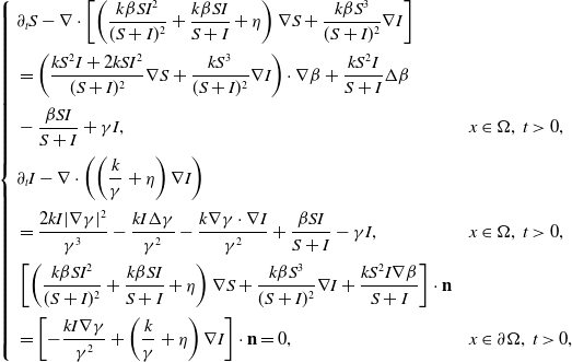 \begin{equation} \left \{\begin{aligned} &\partial _t S-\nabla \cdot \left [\left (\frac {k\beta SI^2}{(S+I)^2}+\frac {k\beta SI}{S+I}+\eta \right )\nabla S +\frac {k\beta S^3}{(S+I)^2}\nabla I\right ]\\[2pt] &=\left (\frac {k S^2I+2kSI^2}{(S+I)^2}\nabla S+\frac {k S^3}{(S+I)^2}\nabla I\right )\cdot \nabla \beta +\frac {k S^2 I}{S+I}\Delta \beta \\[2pt] &-\frac {\beta SI}{S+I}+\gamma I,\ & x&\in \Omega ,\ t\gt 0,\\[2pt] &\partial _t I-\nabla \cdot \left (\left (\frac {k}{\gamma }+\eta \right )\nabla I\right )\\[2pt] &=\frac {2kI|\nabla \gamma |^2}{\gamma ^3}-\frac {kI\Delta \gamma }{\gamma ^2}-\frac {k\nabla \gamma \cdot \nabla I}{\gamma ^2}+\frac {\beta SI}{S+I}-\gamma I,\ & x&\in \Omega ,\ t\gt 0,\\[2pt] &\displaystyle \left [\left (\frac {k\beta SI^2}{(S+I)^2}+\frac {k\beta SI}{S+I}+\eta \right )\nabla S +\frac {k\beta S^3}{(S+I)^2}\nabla I+\frac {kS^2I\nabla \beta }{S+I}\right ]\cdot \mathbf{n}\\[2pt] &=\left [-\frac {kI\nabla \gamma }{\gamma ^2}+\left (\frac {k}{\gamma }+\eta \right )\nabla I\right ]\cdot \mathbf{n}=0,\ & x&\in \partial \Omega ,\ t\gt 0, \end{aligned}\right . \end{equation}
and the steady state of (5.2) is shown in Figure 3(e).
If the diffusion rate of infected individuals is $g(\gamma , I)=k/\gamma I+\eta$
, the
$g(\gamma , I)=k/\gamma I+\eta$
, the $I$
-equation in (5.1) will be replaced by
$I$
-equation in (5.1) will be replaced by
 \begin{equation} \partial _t I-\nabla \cdot \left (\left (\frac {k}{\gamma I}+\eta \right )\nabla I\right )=\frac {\beta SI}{S+I}-\gamma I,\ x\in \Omega ,\ t\gt 0 \end{equation}
with the same boundary condition in (5.1). The $I$
-equation in (5.2) will be replaced by
$I$
-equation in (5.2) will be replaced by
 \begin{equation*}\partial _t I-\eta \Delta I\\ =2k\gamma ^{-3}|\nabla I|^2-k\gamma ^{-2}\Delta \gamma +\frac {\beta SI}{S+I}-\gamma I,\ x\in \Omega ,\ t\gt 0\end{equation*}
with the boundary condition
 \begin{equation*}({-}k\gamma ^{-2}\nabla \gamma +\eta \nabla I)\cdot \mathbf{n}=0.\end{equation*}
There is the singularity in the diffusion rate of (5.3), since $I$
can be zero at the steady state. The corresponding steady states are shown in Figure 3(c) and (f), respectively.
$I$
can be zero at the steady state. The corresponding steady states are shown in Figure 3(c) and (f), respectively.
The distribution of steady states for $k=1$
,
$k=1$
, $\eta =0.0001$
,
$\eta =0.0001$
, $\beta =6\cos x+6.6$
,
$\beta =6\cos x+6.6$
, $\gamma =\cos x+1.5$
.
$\gamma =\cos x+1.5$
.
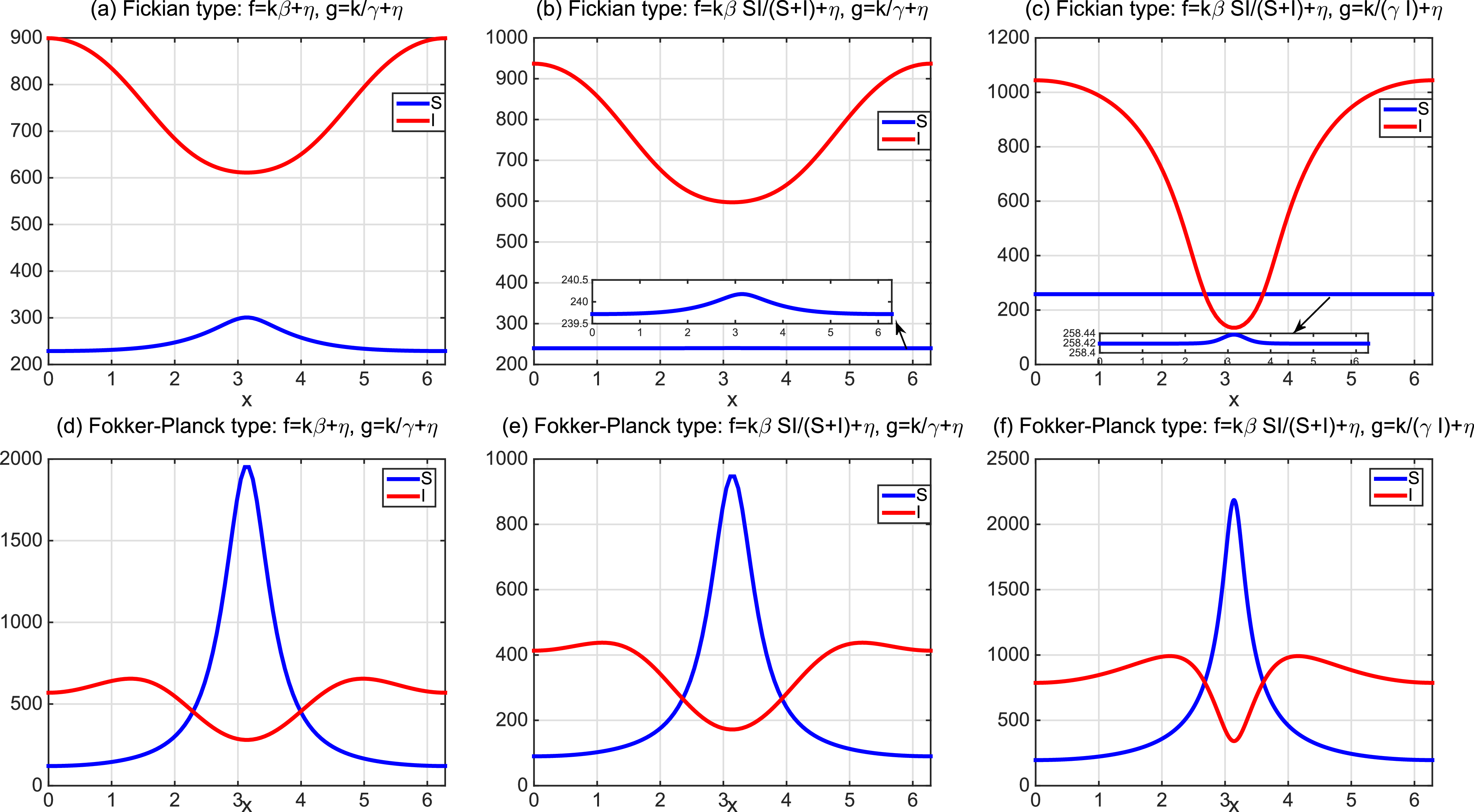
In this case, the infection and recovery rate peaks at the same position (see Figure 2(a)). It can be observed from Figure 3(b) and (c) that Fickian law contributes to the spatial homogenization of the distribution of susceptible individuals significantly in the quasilinear systems (5.1) and (5.3), while the Fokker–Planck type never gives rise to this phenomenon. The distribution in Figure 3 for semilinear systems is similar to that for quasilinear systems.
By observing Table 1, we can find that the Fokker–Planck-type law of diffusion helps the spatial segregation of susceptible and infected individuals since the values of $\chi$
are negative for this type. As a consequence, the final infection fraction is relatively small compared with the Fickian law. There is also a segregation phenomenon for the Fickian law if the diffusion rate of infected individuals depends on new recovery cases. Though the segregation occurs, the infection fraction is high, which can be attributed to the high homogenization of susceptible individuals.
$\chi$
are negative for this type. As a consequence, the final infection fraction is relatively small compared with the Fickian law. There is also a segregation phenomenon for the Fickian law if the diffusion rate of infected individuals depends on new recovery cases. Though the segregation occurs, the infection fraction is high, which can be attributed to the high homogenization of susceptible individuals.
Segregation indices and infection fraction of $k=1$
,
$k=1$
, $\eta =0.0001$
,
$\eta =0.0001$
, $\beta =6\cos x+6.6$
,
$\beta =6\cos x+6.6$
, $\gamma =\cos x+1.5$
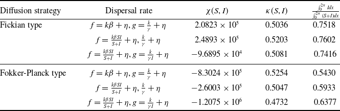
We now consider the case where the infection rate is the lowest at $x=\pi$
, while the recovery rate is the lowest at
$x=\pi$
, while the recovery rate is the lowest at $x=\frac {3\pi }{2}$
(see Figure 2(b)). The corresponding steady states are displayed in Figure 4. It can be seen from Table 2 that only the value of
$x=\frac {3\pi }{2}$
(see Figure 2(b)). The corresponding steady states are displayed in Figure 4. It can be seen from Table 2 that only the value of $\chi$
for model (5.1) is positive, implying that only this model performs no segregation. For the negative
$\chi$
for model (5.1) is positive, implying that only this model performs no segregation. For the negative $\chi$
, the values of
$\chi$
, the values of $\kappa$
for the Fokker–Planck type are bigger than those for the Fickian type, leading to better spatial segregation and a smaller infection fraction for the Fokker–Planck type. The segregation is perfect for the case
$\kappa$
for the Fokker–Planck type are bigger than those for the Fickian type, leading to better spatial segregation and a smaller infection fraction for the Fokker–Planck type. The segregation is perfect for the case $g=k/(\gamma I)+\eta$
of the Fokker–Planck type due to
$g=k/(\gamma I)+\eta$
of the Fokker–Planck type due to $\kappa =0.9626$
being close to one. As a consequence, the infected fraction is close to zero in such a case.
$\kappa =0.9626$
being close to one. As a consequence, the infected fraction is close to zero in such a case.
Segregation indices and infection fraction of $k=1$
,
$k=1$
, $\eta =0.0001$
,
$\eta =0.0001$
, $\beta =6\cos x+6.6$
,
$\beta =6\cos x+6.6$
, $\gamma =\sin x+1.5$
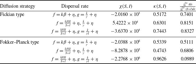
The distribution of steady states for $k=1$
,
$k=1$
, $\eta =0.0001$
,
$\eta =0.0001$
, $\beta =6\cos x+6.6$
,
$\beta =6\cos x+6.6$
, $\gamma =\sin x+1.5$
.
$\gamma =\sin x+1.5$
.
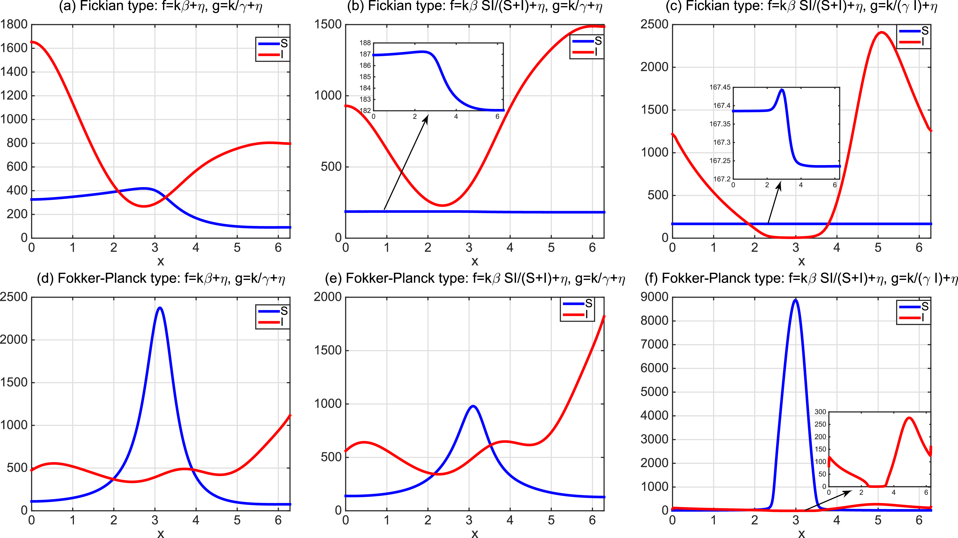
The distribution of steady states for $k=1$
,
$k=1$
, $\eta =0.0001$
,
$\eta =0.0001$
, $\beta =5e^{-160(x-0.2)^2}+4$
,
$\beta =5e^{-160(x-0.2)^2}+4$
, $\gamma =5e^{-160(x-0.8)^2}+2$
.
$\gamma =5e^{-160(x-0.8)^2}+2$
.
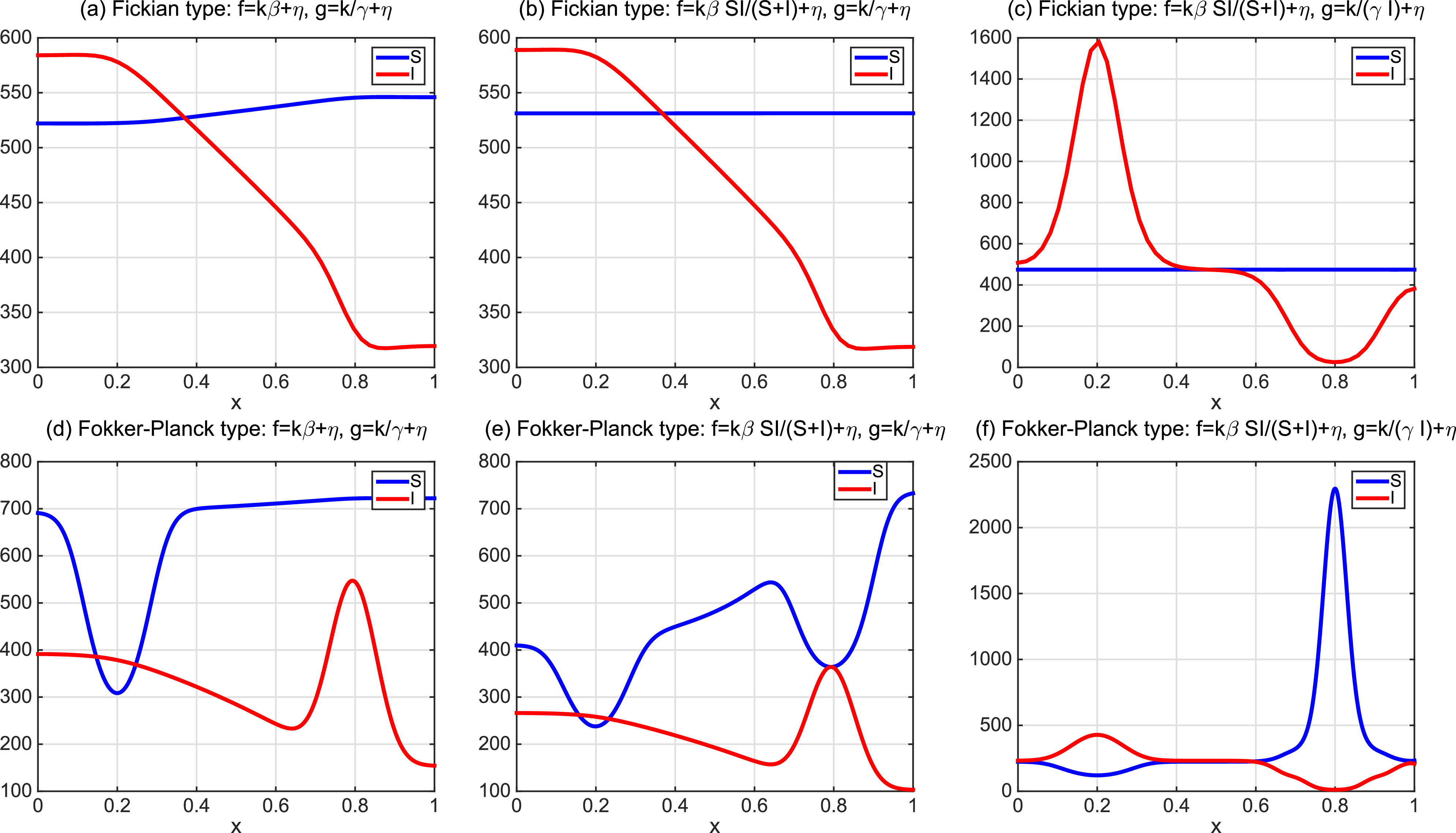
The steady-state distributions among different models exhibit significant differences. Susceptible individuals show homogeneous spatial distribution in the Fickian type, especially in quasilinear systems, while displaying heterogeneous distribution in the Fokker–Planck type. In Figure 4(a)(b)(d)(e), the density of infected individuals is not the highest at the position $x=\frac {3\pi }{2}$
where the recovery rate is the lowest. However, in Figure 4(c) and (f), the density of infected individuals is the lowest around this position, suggesting that new recovery cases are more helpful to individual movement. When the diffusion rate of infected individuals is
$x=\frac {3\pi }{2}$
where the recovery rate is the lowest. However, in Figure 4(c) and (f), the density of infected individuals is the lowest around this position, suggesting that new recovery cases are more helpful to individual movement. When the diffusion rate of infected individuals is $g=k/(\gamma I)+\eta$
, a disease-free region emerges around
$g=k/(\gamma I)+\eta$
, a disease-free region emerges around $x=\pi$
for both types of diffusion laws. Interestingly, there is a notable aggregation of susceptible individuals in the disease-free region for the Fokker–Planck type. This corresponds to the tendency of susceptible individuals to move towards disease-free regions to avoid infection.
$x=\pi$
for both types of diffusion laws. Interestingly, there is a notable aggregation of susceptible individuals in the disease-free region for the Fokker–Planck type. This corresponds to the tendency of susceptible individuals to move towards disease-free regions to avoid infection.
To describe the infection and recovery rates more realistic, we choose
 \begin{equation*}\beta =5e^{-160(x-0.2)^2}+4,\ \gamma =5e^{-160(x-0.8)^2}+2,\ x\in (0,1),\end{equation*}
which are shown in Figure 2(c). The infection rate peaks at $x=0.2$
, corresponding to the indoor playground with the high disease infection rate, while the recovery rate reaches its maximum at
$x=0.2$
, corresponding to the indoor playground with the high disease infection rate, while the recovery rate reaches its maximum at $x=0.8$
, denoting the hospital with enough medical resources. The distribution of susceptible individuals remains spatially homogeneous, while infected individuals exhibit sensitivity to the infection and recovery rates in Fickian law of diffusion (see Figure 5(a), (b) and (c)). The density of infectives is the highest at
$x=0.8$
, denoting the hospital with enough medical resources. The distribution of susceptible individuals remains spatially homogeneous, while infected individuals exhibit sensitivity to the infection and recovery rates in Fickian law of diffusion (see Figure 5(a), (b) and (c)). The density of infectives is the highest at $x=0.2$
and the lowest at
$x=0.2$
and the lowest at $x=0.8$
for the Fickian type. However, in the Fokker–Planck type, the density of infectives is the highest at
$x=0.8$
for the Fickian type. However, in the Fokker–Planck type, the density of infectives is the highest at $x=0.8$
(see Figure 5(d) and (e)) when
$x=0.8$
(see Figure 5(d) and (e)) when $g$
depends on the recovery rate, while it is the lowest at this position when
$g$
depends on the recovery rate, while it is the lowest at this position when $g$
depends on new recovery cases (see Figure 5(f)). Consequently, optimal individual movement is observed in Figure 5(f), where a disease-free region occurs around
$g$
depends on new recovery cases (see Figure 5(f)). Consequently, optimal individual movement is observed in Figure 5(f), where a disease-free region occurs around $x=0.8$
.
$x=0.8$
.
The spatial separation between the locations with the highest infection and recovery rates leads to the spatial segregation of susceptible and infected individuals in this case, as indicated by the consistently negative values of $\chi$
in Table 3. The infection fraction in the Fokker–Planck type is smaller than that in the Fickian type.
$\chi$
in Table 3. The infection fraction in the Fokker–Planck type is smaller than that in the Fickian type.
Segregation indices and infection fraction of $k=1$
,
$k=1$
, $\eta =0.0001$
,
$\eta =0.0001$
, $\beta =5e^{-160(x-0.2)^2}+4$
,
$\beta =5e^{-160(x-0.2)^2}+4$
, $\gamma =5e^{-160(x-0.8)^2}+2$
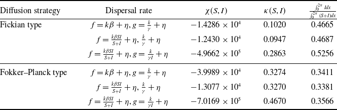
5.2. Exponential and algebraic dependencies
In this subsection, we consider the cases where the diffusion rates are in exponential and algebraic forms. For Fickian law of diffusion with exponential-dependent dispersal rate, model (1.5) becomes
 \begin{equation} \left \{\begin{aligned} &\partial _t S-\nabla \cdot \left (\eta e^{\frac {k\beta SI}{S+I}}\nabla S \right )=-\frac {\beta SI}{S+I}+\gamma I,\ & x&\in \Omega ,\ t\gt 0,\\ &\partial _t I-\nabla \cdot \left (\eta e^{-k\gamma }\nabla I\right )=\frac {\beta SI}{S+I}-\gamma I,\ & x&\in \Omega ,\ t\gt 0,\\ &\displaystyle \nabla S\cdot \mathbf{n}=\nabla I\cdot \mathbf{n}=0,\ & x&\in \partial \Omega ,\ t\gt 0. \end{aligned}\right . \end{equation}
For the Fokker–Planck type law of diffusion, model (1.6) can be written as
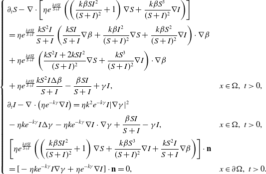 \begin{equation} \left \{\begin{aligned} &\partial _t S-\nabla \cdot \left [\eta e^{\frac {k\beta SI}{S+I}}\left (\left (\frac {k\beta SI^2}{(S+I)^2}+1\right )\nabla S+\frac {k\beta S^3}{(S+I)^2}\nabla I\right )\right ]\\[3pt] &=\eta e^{\frac {k\beta SI}{S+I}}\frac {kS^2I}{S+I}\left (\frac {kSI}{S+I}\nabla \beta +\frac {k\beta I^2}{(S+I)^2}\nabla S+\frac {k\beta S^2}{(S+I)^2}\nabla I\right )\cdot \nabla \beta \\[3pt] &+\eta e^{\frac {k\beta SI}{S+I}}\left (\frac {kS^2I+2kSI^2}{(S+I)^2}\nabla S+\frac {kS^3}{(S+I)^2}\nabla I\right )\cdot \nabla \beta \\[3pt] &+\eta e^{\frac {k\beta SI}{S+I}}\frac {kS^2I\Delta \beta }{S+I}-\frac {\beta SI}{S+I}+\gamma I,\ & x&\in \Omega ,\ t\gt 0,\\[3pt] &\partial _t I-\nabla \cdot \left (\eta e^{-k\gamma }\nabla I\right )=\eta k^2e^{-k\gamma } I|\nabla \gamma |^2\\[3pt] &-\eta ke^{-k\gamma }I\Delta \gamma -\eta ke^{-k\gamma }\nabla I\cdot \nabla \gamma +\frac {\beta SI}{S+I}-\gamma I,\ & x&\in \Omega ,\ t\gt 0,\\[3pt] &\displaystyle \left [\eta e^{\frac {k\beta SI}{S+I}}\left (\left (\frac {k\beta SI^2}{(S+I)^2}+1\right )\nabla S+\frac {k\beta S^3}{(S+I)^2}\nabla I+\frac {kS^2I}{S+I}\nabla \beta \right )\right ]\cdot \mathbf{n}\\[3pt] &=[-\eta ke^{-k\gamma }I\nabla \gamma +\eta e^{-k\gamma }\nabla I]\cdot \mathbf{n}=0,\ & x&\in \partial \Omega ,\ t\gt 0. \end{aligned}\right . \end{equation}
If the diffusion rate of infected individuals is $g(\gamma , I)$
, the
$g(\gamma , I)$
, the $I$
-equation in (5.4) will be replaced by
$I$
-equation in (5.4) will be replaced by
 \begin{equation*}\partial _t I-\nabla \cdot \left (\eta e^{-k\gamma I}\nabla I\right )=\frac {\beta SI}{S+I}-\gamma I,\ x\in \Omega ,\ t\gt 0\end{equation*}
with the same boundary condition in (5.4). The $I$
-equation in (5.5) will be replaced by
$I$
-equation in (5.5) will be replaced by
 \begin{eqnarray*} & &\partial _t I-\nabla \cdot \left (\eta e^{-k\gamma I}(1-k\gamma I)\nabla I\right )=\eta e^{-k\gamma I}(k^2I^3\nabla \gamma +k^2\gamma I^2\nabla I)\nabla \gamma -2\eta k e^{-k\gamma I} I\nabla \gamma \cdot \nabla I\\ &&-\eta k e^{-k\gamma I}I^2\Delta \gamma +\frac {\beta SI}{S+I}-\gamma I,\ x\in \Omega ,\ t\gt 0 \end{eqnarray*}
with the boundary condition
 \begin{equation*}\left [-\eta ke^{-k\gamma I}I^2\nabla \gamma +\eta e^{-k\gamma I}(1-k\gamma I)\nabla I\right ]\cdot \mathbf{n}=0.\end{equation*}
When we take algebraically dependent functions for the diffusion rates, the steady states for models (1.3) and (1.4) are illustrated in Figure 6(a)(d). For Fickian law of diffusion, system (1.5) becomes
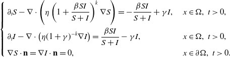 \begin{equation} \left \{\begin{aligned} &\partial _t S-\nabla \cdot \left (\eta \left (1+\frac {\beta SI}{S+I}\right )^k\nabla S \right )=-\frac {\beta SI}{S+I}+\gamma I,\ & x&\in \Omega ,\ t\gt 0,\\ &\partial _t I-\nabla \cdot \left (\eta (1+\gamma )^{-k}\nabla I\right )=\frac {\beta SI}{S+I}-\gamma I,\ & x&\in \Omega ,\ t\gt 0,\\ &\displaystyle \nabla S\cdot \mathbf{n}=\nabla I\cdot \mathbf{n}=0,\ & x&\in \partial \Omega ,\ t\gt 0. \end{aligned}\right . \end{equation}
For the Fokker–Planck law of diffusion, system (1.6) is written as
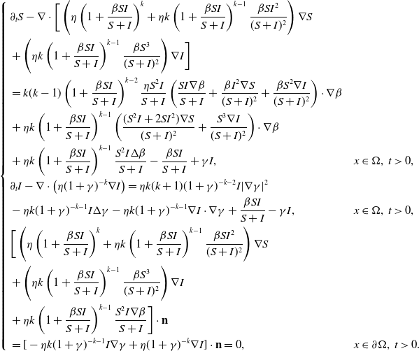 \begin{equation} \left \{\begin{aligned} &\partial _t S-\nabla \cdot \bigg [\left (\eta \left (1+\frac {\beta SI}{S+I}\right )^k+\eta k\left (1+\frac {\beta SI}{S+I}\right )^{k-1}\frac {\beta SI^2}{(S+I)^2}\right )\nabla S\\ &+\left (\eta k\left (1+\frac {\beta SI}{S+I}\right )^{k-1}\frac {\beta S^3}{(S+I)^2}\right )\nabla I\bigg ]\\ &=k(k-1)\left (1+\frac {\beta SI}{S+I}\right )^{k-2}\frac {\eta S^2I}{S+I}\left (\frac {SI\nabla \beta }{S+I}+\frac {\beta I^2\nabla S}{(S+I)^2}+\frac {\beta S^2\nabla I}{(S+I)^2}\right )\cdot \nabla \beta \\ &+\eta k\left (1+\frac {\beta SI}{S+I}\right )^{k-1}\left (\frac {(S^2I+2SI^2)\nabla S}{(S+I)^2}+\frac {S^3\nabla I}{(S+I)^2}\right )\cdot \nabla \beta \\ &+\eta k\left (1+\frac {\beta SI}{S+I}\right )^{k-1}\frac {S^2I\Delta \beta }{S+I}-\frac {\beta SI}{S+I}+\gamma I,\ & x&\in \Omega ,\ t\gt 0,\\ &\partial _t I-\nabla \cdot \left (\eta (1+\gamma )^{-k}\nabla I\right )=\eta k(k+1)(1+\gamma )^{-k-2}I|\nabla \gamma |^2\\ &-\eta k(1+\gamma )^{-k-1}I\Delta \gamma -\eta k(1+\gamma )^{-k-1}\nabla I\cdot \nabla \gamma +\frac {\beta SI}{S+I}-\gamma I,\ & x&\in \Omega ,\ t\gt 0,\\ &\displaystyle \bigg [\left (\eta \left (1+\frac {\beta SI}{S+I}\right )^k+\eta k\left (1+\frac {\beta SI}{S+I}\right )^{k-1}\frac {\beta SI^2}{(S+I)^2}\right )\nabla S\\ &+\left (\eta k\left (1+\frac {\beta SI}{S+I}\right )^{k-1}\frac {\beta S^3}{(S+I)^2}\right )\nabla I\\ &+\eta k\left (1+\frac {\beta SI}{S+I}\right )^{k-1}\frac {S^2I\nabla \beta }{S+I}\bigg ]\cdot \mathbf{n}\\ &=[-\eta k(1+\gamma )^{-k-1}I\nabla \gamma +\eta (1+\gamma )^{-k}\nabla I]\cdot \mathbf{n}=0,\ & x&\in \partial \Omega ,\ t\gt 0. \end{aligned}\right . \end{equation}
The steady states of systems (5.6) and (5.7) are shown in Figure 6(b)–(e). If the diffusion rate of infected individuals is $g(\gamma , I)$
, the
$g(\gamma , I)$
, the $I$
-equation in (5.6) will be replaced by
$I$
-equation in (5.6) will be replaced by
 \begin{equation*}\partial _t I-\nabla \cdot \left (\eta (1+\gamma I)^{-k}\nabla I\right )=\frac {\beta SI}{S+I}-\gamma I,\ x\in \Omega ,\ t\gt 0\end{equation*}
with the same boundary condition in (5.6). The $I$
-equation in (5.7) will be replaced by
$I$
-equation in (5.7) will be replaced by
 \begin{eqnarray*} & &\partial _t I-\nabla \cdot \left [\eta \left ((1+\gamma I)^{-k}-k(1+\gamma I)^{-k-1}\gamma I\right )\nabla I\right ]\\ &=&\eta k(k+1)(1+\gamma I)^{-k-2}(\gamma I^2\nabla I+I^3\nabla \gamma )\nabla \gamma -2\eta k(1+\gamma I)^{-k-1}I\nabla \gamma \cdot \nabla I\\ &&-\eta k(1+\gamma I)^{-k-1}I^2\Delta \gamma +\frac {\beta SI}{S+I}-\gamma I,\ x\in \Omega ,\ t\gt 0 \end{eqnarray*}
with the boundary condition
 \begin{equation*}\left [-\eta k(1+\gamma I)^{-k-1}I^2\nabla \gamma +\eta ((1+\gamma I)^{-k}-k(1+\gamma I)^{-k-1}\gamma I)\nabla I\right ]\cdot \mathbf{n}=0.\end{equation*}
The corresponding numerical results are given in Figure 6(c) and (f).
The simulation results for exponentially dependent diffusion closely resemble those for algebraically dependent diffusion. Therefore, we only present the numerical results for the algebraic case, as shown in Figure 6. In the Fickian type, the spatial distribution is similar for both semilinear and quasilinear systems. Conversely, in the Fokker–Planck type, susceptible individuals appear to exhibit heterogeneous distribution. From Table 4, there is no segregation in quasilinear systems with Fickian diffusion, whereas segregation occurs in the Fokker–Planck type. The infection fraction is minimized when $g=\eta (1+\gamma I)^{-k}$
for the Fokker–Planck type.
$g=\eta (1+\gamma I)^{-k}$
for the Fokker–Planck type.
The distribution of steady states for $k=0.1$
,
$k=0.1$
, $\eta =1$
,
$\eta =1$
, $\beta =6\cos x+6.6$
,
$\beta =6\cos x+6.6$
, $\gamma =\cos x+1.5$
.
$\gamma =\cos x+1.5$
.
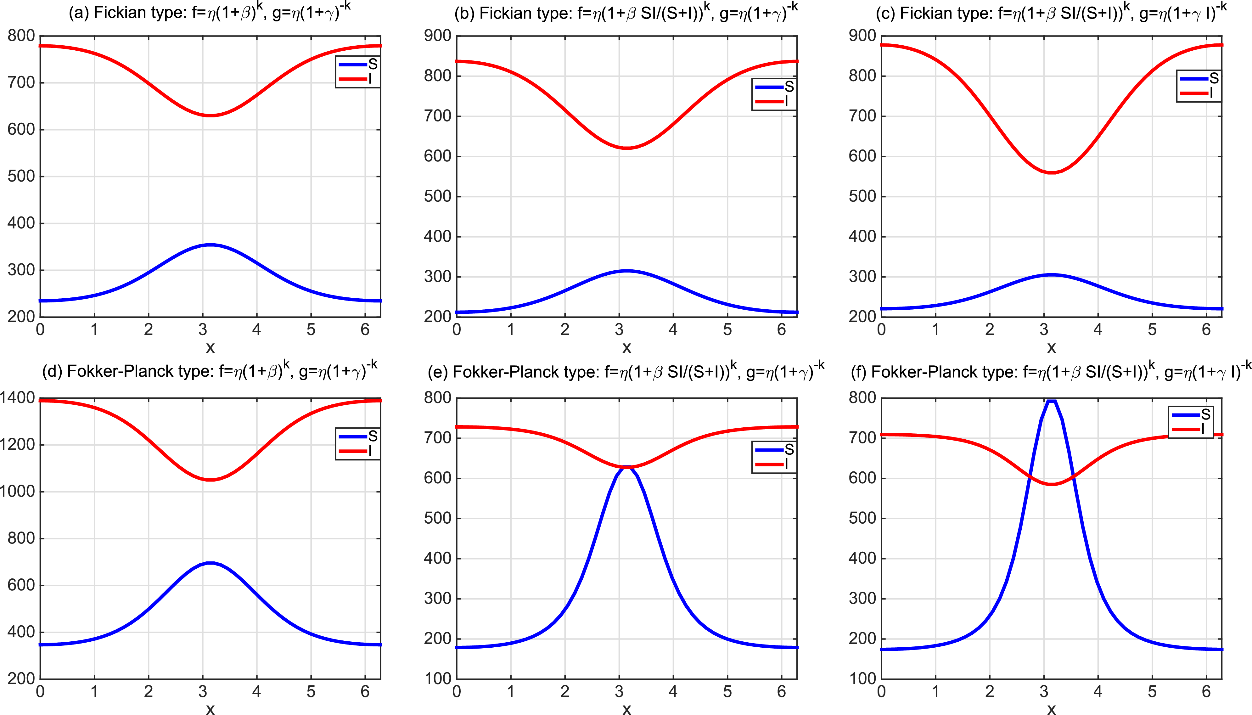
Segregation indices and infection fraction of $k=0.1$
,
$k=0.1$
, $\eta =1$
,
$\eta =1$
, $\beta =6\cos x+6.6$
,
$\beta =6\cos x+6.6$
, $\gamma =\cos x+1.5$
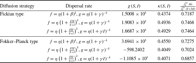
Upon comparing the numerical simulations (including these in [Reference Wang, Wang and Kim29]) of the semilinear systems (1.3) and (1.4) with the quasilinear systems (1.5) and (1.6), we observe that susceptible individuals display spatial homogeneity in the quasilinear systems with Fickian law of diffusion, and the disease-free region appears in quasilinear systems with the Fokker–Planck-type law of diffusion.
6. Discussion
In this paper, adopting Fickian and the Fokker–Planck-type laws of diffusion, we investigated two SIS epidemic models established by strongly coupled quasilinear parabolic equations, where the dispersal rate of susceptible individuals depends on new infection cases, while the dispersal rate of infected individuals depends on the recovery rate or new recovery cases. Zero-flux boundary conditions are imposed to maintain the total population size. We theoretically analysed the scenario in which the dispersal rate of infected individuals depends on the recovery rate. Meanwhile, the scenario where the dispersal rate of infected individuals depends on new recovery cases has been considered mainly through numerical methods.
In the case where the dispersal rate of infected individuals depends on the recovery rate, our initial focus was on examining the global existence of solutions for (1.5) and (1.6). Theorems2.1 and 2.2 confirmed that the formulated systems are well-defined. As the basic reproduction number holds a crucial role in disease control, we established the monotonicity and asymptotics of it by considering either an exponential or algebraic form for the dispersal rate of infected individuals, given by Propositions3.2 and 3.4. The extinction and uniform persistence of the disease were explored in terms of the basic reproductions. The threshold dynamics for (1.5) were demonstrated in Proposition4.2. In fact, (1.6) can be regarded as a cross-diffusion model with a position-dependent cross-diffusion rate. The stability analysis of the constant equilibria was carried out for this model, and the threshold dynamics for (1.6) were established in Theorems4.2 and 4.3 by assuming that $\beta$
and
$\beta$
and $\gamma$
are constant on the domain. Figure 1 confirms the corresponding results.
$\gamma$
are constant on the domain. Figure 1 confirms the corresponding results.
To reveal more epidemic dynamics of the systems with the dispersal rate of infected individuals depending on new recovery cases and compare spatial segregation between susceptible and infected individuals driven by the two types of diffusion pattern, we performed a series of numerical simulations for the steady states in terms of the dependence of the dispersal rate on the infection or recovery rate and new infection or recovered cases. We observed that Fickian law of diffusion always contributes to the spatial homogenization of susceptible individuals in the quasilinear parabolic systems, whereas the Fokker–Planck-type law never shows this effect. When we separated the highest infection rate position and recovery rate position, we found that the disease-free region appears around positions with the highest recovery rate or with the lowest infection rate in the systems where the diffusion rate of infected individuals depends on new recovery cases. More intriguingly, in the Fokker–Planck type with the dispersal rate of infected individuals depending on new recovery cases, there is a notable tendency for susceptible individuals to aggregate in the disease-free region. In contrast, the distribution of susceptible individuals remains spatially homogeneous in the Fickian type. Therefore, it appears that the Fokker–Planck-type law exhibits a more ‘intelligent’ behaviour. In the exponentially and algebraically dependent patterns, the steady states behave similar distribution. Spatial segregation is more likely to occur in the quasilinear parabolic systems with the Fokker–Planck-type diffusion law.
The interesting phenomena arising from numerical simulations promote some open questions, especially on the distribution of steady states. What causes the homogenization of susceptible individuals in Fickian law of diffusion? How can we verify the existence of the disease-free region at the steady state and why do susceptible individuals aggregate at the disease-free region in Figure 4(f) and Figure 5(f)? We shall examine the steady states of such quasilinear parabolic systems in the future for a comprehensive understanding of these questions.
Data availability statement
Data sharing was not applicable to this article as no datasets were generated or analysed during the current study.
Funding statement
The research of Guodong Liu was partially supported by the China Postdoctoral Science Foundation (Nos. 2024M761932, GZC20252017). The research of Hao Wang was partially supported by the Natural Sciences and Engineering Research Council of Canada (Individual Discovery Grant RGPIN-2025-05734) and the Canada Research Chairs program (Tier 1 Canada Research Chair Award). The research of Xiaoyan Zhang was partially supported by the Natural Science Foundation of Shandong Province (No. ZR2021MA062).
Competing interests
The authors declare that they have no conflict of interest.


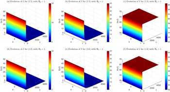


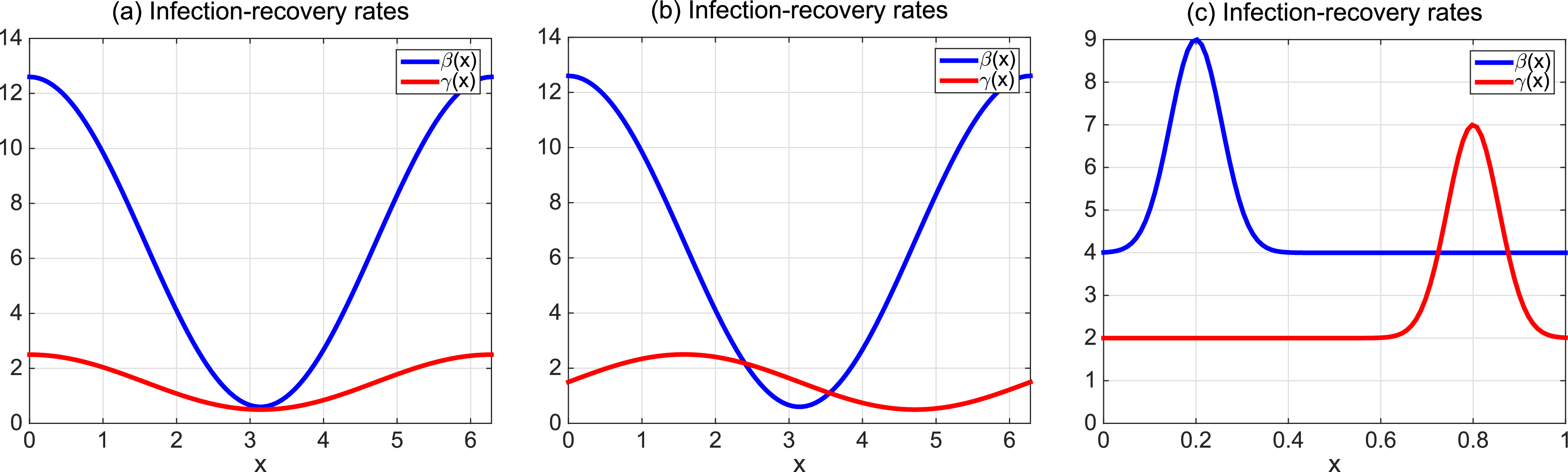


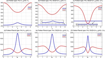


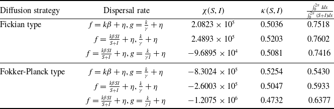


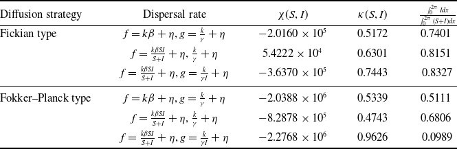


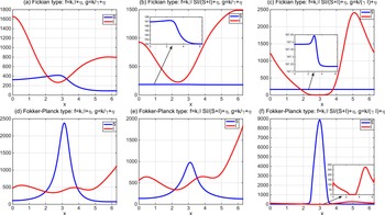


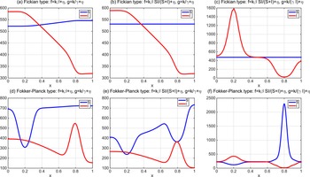


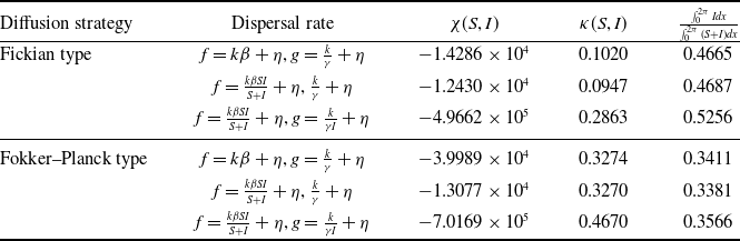


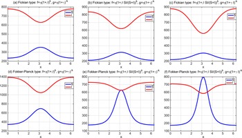


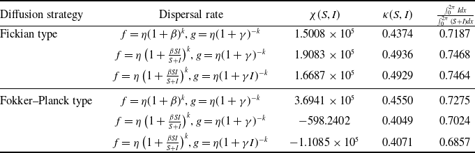


 Open access

