





1. Introduction
Downstream of the location where confluent flows come into contact, a mixing interface (MI) region develops between the two streams. This region is characterized by a large momentum redistribution and mass exchange between the confluent flows and by the generation of large-scale coherent structures (e.g. Sukhodolov & Schnauder Reference Sukhodolov and Schnauder2010; Constantinescu Reference Constantinescu2014; Lam, Ghidaoui & Kolyshkin Reference Lam, Ghidaoui and Kolyshkin2016; Sukhodolov et al. Reference Sukhodolov, Krick, Sukhodolova, Cheng, Rhoads and Constantinescu2017; Cheng & Constantinescu Reference Cheng and Constantinescu2020a). These structures play a major role in enhancing mixing between the confluent flows and affect entrainment and transport of particulates (e.g. in the case the confluent flows move over a loose bed).
In the case of two parallel streams of unequal velocities but of equal densities and for deep-flow conditions, the MI is a mixing layer that contains Kelvin–Helmholtz (KH) vortices generated by the mean shear between the two streams. The streamwise growth of the mixing layer width, δ(x), is unbounded (e.g. Winant & Browand Reference Winant and Browand1974; Lesieur et al. Reference Lesieur, Staquet, Le Roy and Comte1988; Moser & Rogers Reference Moser and Rogers1993). In many geosciences and environmental fluid mechanics applications, the mixing layer develops over a smooth or rough bottom surface in a high-aspect-ratio channel. The most common example is that of river confluences where the channel mean aspect ratio is generally larger than 20 and the incoming streams are often characterized by different velocities, directions, temperatures and/or suspended sediment loads. If the velocity difference between the incoming flows is large and their density contrast is negligible, the KH vortices developing between parallel streams attain sizes that are much larger than the mean channel depth. Once that happens, the dynamics of these vortices is strongly affected by bed friction and the rate of growth of the mixing layer width, δ, reduces with respect to that of a classical (deep) mixing layer (Chu & Babarutsi Reference Chu and Babarutsi1988; Babarutsi & Chu Reference Babarutsi and Chu1998; Uijttewaal & Booij Reference Uijttewaal and Booij2000; Sukhodolov & Schnauder Reference Sukhodolov and Schnauder2010; Lam et al. Reference Lam, Ghidaoui and Kolyshkin2016; Cheng & Constantinescu Reference Cheng and Constantinescu2020a). Such phenomena are similar to those observed for other types of shallow flows where large-scale, quasi-two-dimensional (quasi-2-D) vortices are generated (Socolofsky & Jirka Reference Socolofsky and Jirka2004; Chu Reference Chu2014). For example, shallow wakes are also subject to similar effects that lead to a sharp decay of their rate of growth at large distances from the obstacle with respect to deep wakes (e.g. see; Negretti et al. Reference Negretti, Vignoli, Tubino and Brocchini2006; Rockwell Reference Rockwell2008). Moreover, the velocity difference between the two streams is monotonically decreasing with the distance from the mixing layer origin and the streamwise variation of the shift of the mixing layer centreline, lcy, is nonlinear and asymptotically reaches a constant value (Cushman-Roisin & Constantinescu Reference Cushman-Roisin and Constantinescu2020). Such a mixing layer is characterized as being shallow.
Cheng & Constantinescu (Reference Cheng and Constantinescu2020a) identified several regimes characterizing the spatial development of a shallow mixing layer between parallel streams with no density contrast. Near its origin, the shallow mixing layer behaves as a deep mixing layer. Once the KH vortices become sufficiently large such that their dynamics is significantly affected by stabilization effects associated with bed friction and vortex stretching, they start behaving like quasi-2-D vortices. The mixing layer enters a transitions regime characterized by a loss of the coherence of the quasi-2-D KH vortices that are still undergoing vortex pairing. As a result of the loss of coherence of the KH vortices and reduced mean shear across the mixing layer, the growth of δ in the transition regime is less than linear. Once vortex pairing between successive KH vortices ceases, the mixing layers enters the quasi-equilibrium regime. As the KH vortices are destroyed, the rates of growth of δ and lcy further decay compared with the values observed over the transition regime such that both δ and lcy asymptotically approach constant values (zero-growth).
Recent studies conducted at natural river confluences with a low degree of bed discordance and negligible density contrast between the confluent flows (Constantinescu et al. Reference Constantinescu, Miyawaki, Rhoads and Sukhodolov2012) have shown that the MI contains mostly co-rotating vortices (KH mode is dominant, MI resembles a shallow mixing layer) provided that the mean velocities of the incoming streams are not close. If the velocities of the two streams are close, then the MI generally contains counter-rotating vortices forming by the interaction of the separated shear layers on the two sides of the confluence apex. For such MIs, the wake mode is dominant. Besides the vertically oriented vortices inside the MI, other coherent structures and cells of secondary flow can play an important role in mixing at the confluence of two streams. They include the formation of large recirculation cells of the first kind associated with curvature effects as the flows in the incoming streams align with the MI downstream of the confluence apex, similar to the ones forming in curved open channels (Kashyap et al. Reference Kashyap, Constantinescu, Rennie, Post and Townsend2012). Such cells are absent in the case of confluences between parallel streams. However, the tilt of the MI toward one side can induce weak secondary flow cells of the second kind due to turbulence anisotropy. These cells can reduce transverse mixing (Lyubimova et al. Reference Lyubimova, Lepikhin, Parshakova, Gualtieri, Lane and Roux2019). Finally, streamwise-oriented vortical (SOV) cells are generally observed in the vicinity of the MI at high-angle confluences with a concordant bed (Constantinescu et al. Reference Constantinescu, Miyawaki, Rhoads and Sukhodolov2012; Cheng & Constantinescu Reference Cheng and Constantinescu2021). Such SOV cells do not form at confluences with a small angle between the incoming streams.
The dynamics and structure of the MI become even more complex once buoyancy starts playing an important role (Laraque, Guyot & Filizola Reference Laraque, Guyot and Filizola2009; Prats et al. Reference Prats, Armengol, Marcé, Sánchez-Juny and Dolz2010; Lyubimova et al. Reference Lyubimova, Lepikhin, Konovalov, Parshakova and Tiunov2014, Reference Lyubimova, Lepikhin, Parshakova, Kolchanov, Gualtieri, Roux and Lane2020; Ramón et al. Reference Ramón, Armengol, Dolz, Prats and Rueda2014; Lewis & Rhoads Reference Lewis and Rhoads2015; Cheng & Constantinescu Reference Cheng and Constantinescu2018; Gualtieri, Ianniruberto & Filizola Reference Gualtieri, Ianniruberto and Filizola2019; Gualtieri et al. Reference Gualtieri, Ianniruberto and Filizola2019; Horna-Munoz et al. Reference Horna-Munoz, Constantinescu, Rhoads, Quinn and Sukhodulov2020). For sufficiently large density contrast between the incoming streams, the rates of mixing between the two streams were found to be quite different from the ones observed for cases with negligible density contrast (Horna-Munoz et al. Reference Horna-Munoz, Constantinescu, Rhoads, Quinn and Sukhodulov2020). Several studies (e.g. see Constantinescu Reference Constantinescu2014; Cheng & Constantinescu Reference Cheng and Constantinescu2020b; Horna-Munoz et al. Reference Horna-Munoz, Constantinescu, Rhoads, Quinn and Sukhodulov2020) have shown that buoyancy effects are significant if the densimetric Froude number  $Fr = {U_0}/{(g|{\rho _{10}} - {\rho _{20}}|/{\rho _0}D)^{1/2}}$ is smaller than 10, or equivalently, the Richardson number, Ri = 1/Fr 2, is larger than 0.01, where g is the gravitational acceleration, ρ 10 and ρ 20 are the constant densities of the two incoming streams, ρ 0 is the mean density, D is the mean flow depth downstream of the confluence apex and U 0 is a velocity scale that characterizes the average streamwise velocity downstream of the confluence apex. For parallel streams separated by a splitter plate (figure 1), U 0 can be estimated as 0.5(U 10 + U 20), where U 10 and U 20 are the velocities of the slower and of the faster incoming stream, respectively, upstream of the end of the splitter plate.
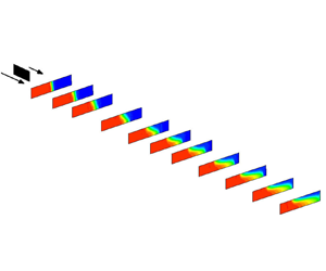
Sketch of the computational domain showing the main dimensions. The incoming parallel streams have velocities U 10 and U 20 and densities ρ 10 and ρ 20 before the end of the splitter plate situated at x = 0. A scalar with C = 100 is introduced at the end of the splitter plate. The circles represent the KH vortices forming over the upstream part of the MI. The middle panel shows the distribution of the passive scalar C in a cross-section of the computational domain for a case with ρ 10 > ρ 20 for which the non-dimensional densities of the incoming streams are TR 10 = 1 and TR 20 = 0. The bottom panel shows the distribution of TR in the same cross-section. The dashed lines show the TR = 0.01 and TR = 0.99 iso-contours based on which one can define the width δ(x) of the MI. The width of the MI based on the TR = 0.5 isoline (solid line) is denoted δ′(x).

The aforementioned studies showed that the main flow feature associated with strong density contrast between the confluent flows was the formation of a near-bed intrusion of heavier fluid in cross-stream planes. In many cases, this was accompanied by the formation of a free-surface intrusion of lighter fluid. The formation of the transverse intrusions observed at natural river confluences is consistent with that of a spatially developing lock-exchange flow. The lateral penetration distance of these intrusions increases with the distance from the confluence apex, similar to the classical case of a temporally evolving lock-exchange flow where the intrusions move away from the position of the initial interface with increasing time (Tokyay, Constantinescu & Meiburg Reference Tokyay, Constantinescu and Meiburg2014). These changes also affect how fast the two streams mix. For example, in the case of a confluence between non-parallel streams with strong density contrast, Constantinescu (Reference Constantinescu2014) found that the MI remained very thin near the free surface for approximately 50D, which would suggest that mixing between the two streams is very weak. However, buoyancy effects increased the total volume of mixed fluid downstream of the confluence apex compared with the case with negligible density contrast, with most of the mixing taking place beneath the free surface. Unfortunately, no laboratory studies were conducted in simplified configurations for cases with strong density contrast between the incoming streams.
The aforementioned findings of field and numerical studies conducted at natural river confluences are the primary motivation of the present study that tries to understand the structure of MIs, mixing processes and sediment entrainment mechanisms in the presence of a strong density contrast between the confluent flows for a canonical case. In the case investigated here, two parallel streams of unequal velocities and unequal densities, initially separated by a splitter plate, come into contact and advance in a wide, long, constant-depth and constant-width channel (no bed discordance) with vertical sidewalls (figure 1). The large channel width should allow for the study of the evolution of the MI over relatively large distances before the effect of the channel sidewalls becomes significant. The complex bathymetry and deformed banks of natural river confluences induce additional flow complexities like generation of large-scale turbulent eddies that interact with the MI eddies and secondary flow due to bank curvature (Gaudet & Roy Reference Gaudet and Roy1995; Leite Ribeiro et al. Reference Leite Ribeiro, Blanckaert, Roy and Schleiss2012). As a result, it is not possible to clearly understand and isolate buoyancy effects induced by density contrast on flow structure and mixing in such complex configurations. Such knowledge on the fundamental flow physics acquired from canonical cases can then serve to understand how other controlling factors (e.g. planform geometry, channel curvature, bathymetry, irregular channel banks) affect flow structure, mixing and sediment transport mechanisms at natural river confluences.
The physics of shallow MIs developing between streams of unequal densities (Ri > 0) and velocities is investigated based on 3-D eddy-resolving numerical simulations using the same solver, turbulence model and type of boundary conditions as the ones used in the companion paper of Cheng & Constantinescu (Reference Cheng and Constantinescu2020a) that focused on shallow mixing layers between parallel streams of equal densities (Ri = 0). Of particular interest is to describe the spatial growth of the MI, the secondary flow structures associated with the lock-exchange-like flow and their effects on the turbulent kinetic energy and bed shear stress distributions, the dynamics of the KH vortices forming close to the splitter plate and the spectral content of the MI. Related goals are to explain how density contrast between the two streams generates new mixing mechanisms and to identify the coherent structures that play an important role in mixing and those that control sediment entrainment in the case of a loose-bed channel. Finally, the present study should allow understanding if density contrast between confluent flows acts toward enhancing or delaying mixing between the two streams. Studies conducted for natural confluences between non-parallel streams suggest that density contrast promotes faster mixing. However, this result may be a consequence of the interplay between buoyancy effects and additional effects associated with flow structures generated in cases when the confluence angle is large (see discussion in Cheng & Constantinescu Reference Cheng and Constantinescu2018; Horna-Munoz et al. Reference Horna-Munoz, Constantinescu, Rhoads, Quinn and Sukhodulov2020) and by secondary flow and mixing generated by a highly deformed bathymetry and irregular bank lines.
The numerical method, boundary conditions and the test cases are presented in § 2. The same section discusses validation of the numerical solver for relevant flows. Section 3 compares the spatial development of the MI in the mean flow for cases with significant density contrast between the incoming streams (Ri = 0.03) with that observed for an equivalent shallow mixing layer forming between streams of equal densities (Ri = 0). Section 4 analyses the dynamics of the main coherent structures generated inside the MI and around it for two cases with Ri = 0.03. The effects of the lock-exchange-like flow on the mean flow and turbulence statistics are discussed in § 5. The effects of density contrast between the incoming streams on mixing and on the sediment entrainment capacity of the flow are discussed in §§ 6 and 7, respectively. Section 8 summarizes the main characteristics of shallow MIs developing between streams of unequal densities and presents some conclusions.
2. Numerical method, test cases and boundary conditions
The incompressible unsteady Navier–Stokes and scalar transport equations are expressed in generalized curvilinear coordinates. The equations are discretized on a collocated mesh. A fractional step method is used to solve the discretized Navier–Stokes equations. Advection–diffusion equations are solved for the non-dimensional density/temperature, TR, the non-dimensional concentration of the passive scalar introduced at the inlets of the two incoming channels, CR, in the simulation with zero temperature difference between the incoming streams and for the non-dimensional concentration of the passive scalar introduced at the end of the splitter plate, C. The Boussinesq approximation is used to account for buoyancy effects on the velocity field. In non-dimensional form, the governing equations are:
 \begin{gather}\frac{{\partial {u_i}}}{{\partial {x_i}}} = 0,\end{gather}
 \begin{gather}\frac{{\partial {u_i}}}{{\partial t}} + \frac{{\partial {u_i}{u_j}}}{{\partial {x_j}}} ={-} \frac{{\partial p}}{{\partial {x_i}}} + \frac{\partial }{{\partial {x_j}}}\left[ {\left( {\frac{1}{{Re}} + {\vartheta_t}} \right)\left( {\frac{{\partial {u_i}}}{{\partial {x_j}}} + \frac{{\partial {u_j}}}{{\partial {x_i}}}} \right)} \right] - Ri\ast TR\ast {\delta_{i3}},\end{gather}
 \begin{gather}\frac{{\partial TR}}{{\partial t}} + \frac{{\partial TR{u_j}}}{{\partial {x_j}}} = \frac{\partial }{{\partial {x_j}}}\left[ {\left( {\frac{1}{{RePr}} + {D_t}} \right)\frac{{\partial TR}}{{\partial {x_j}}}} \right],\end{gather}
 \begin{gather}\frac{{\partial CR}}{{\partial t}} + \frac{{\partial CR{u_j}}}{{\partial {x_j}}} = \frac{\partial }{{\partial {x_j}}}\left[ {\left( {\frac{1}{{RePr}} + {D_t}} \right)\frac{{\partial CR}}{{\partial {x_j}}}} \right],\end{gather}
 \begin{gather}\frac{{\partial C}}{{\partial t}} + \frac{{\partial C{u_j}}}{{\partial {x_j}}} = \frac{\partial }{{\partial {x_j}}}\left[ {\left( {\frac{1}{{ReSc}} + {D_t}} \right)\frac{{\partial C}}{{\partial {x_j}}}} \right],\end{gather}
where the coordinates of the three directions are denoted either (x 1, x 2, x 3) in index notation or (x, y, z) and the Cartesian instantaneous velocity components are denoted either (u 1, u 2, u 3) in index notation or (u, v, w). The mean velocity of the incoming streams, U 0 and the flow depth, D are used to non-dimensionalize all the variables. The other instantaneous variables in (2.1)–(2.5) are the pressure p, the eddy viscosity  ${\vartheta _t}$ and the eddy diffusivity $\; {D_t}$. The Kronecker symbol is δij. The Reynolds number is ${U_0}D/\nu$, where ν is the molecular viscosity. The molecular Prandtl and Schmidt numbers are Pr and Sc, respectively. The scalar TR is used to investigate mixing between the two streams in cases with temperature/density differences. The passive scalar CR is used to investigate mixing for cases with no temperature difference between the two streams. This is why the Schmidt number in (2.4) is taken equal to the molecular Prandtl number in (2.3).
The fifth-order accurate upwind biased scheme is used to discretize the convective terms in the momentum and scalar transport equations. The second-order central scheme is used to discretize the remaining terms in the momentum and pressure-Poisson equations. The discretized equations for the momentum, non-dimensional density/temperature, passive scalars and the turbulent variables are integrated in pseudo-time using the alternate direction implicit approximate factorization scheme. A double time-stepping algorithm is used to solve the unsteady equations. The algorithm is second-order accurate in time and is parallelized using message passing interface. Detached eddy simulation is used to account for the effect of the unresolved turbulent scales on the resolved variables. The delayed detached eddy simulation (DES) version based on the Spalart–Allmaras (SA) model is used to perform the simulations (Spalart Reference Spalart2009). A transport equation is solved for the modified viscosity,  $\tilde{\nu }$ (Spalart Reference Spalart2009). Its values are then used to estimate the (subgrid-scale) eddy viscosity, ${\vartheta _t} = {f_{v1}}\tilde{\nu }$, where fv 1 is a wall-damping function (Spalart Reference Spalart2009). The turbulence length scale in the standard SA model is redefined in DES such that it becomes proportional to the local grid size away from solid surfaces. The values of $\tilde{\nu }$ are set to zero on the smooth surfaces. The eddy diffusivity is assumed to be equal to the eddy viscosity. More details on the flow solver, the SA DES model and its implementation are given in Chang, Constantinescu & Park (Reference Chang, Constantinescu and Park2007b), Keylock, Constantinescu & Hardy (Reference Keylock, Constantinescu and Hardy2012) and Cheng & Constantinescu (Reference Cheng and Constantinescu2018).
In the present simulations with different temperatures in the incoming streams, buoyancy effects are driven by the unequal temperatures of the two incoming streams. The non-dimensional density/temperature is defined as  $TR = ({T_{10}} - T(x,y,z,t))/ ({T_{10}} - {T_{20}})$, where T is the dimensional temperature field and T 10 and T 20 are the temperatures in the two incoming streams. The values of TR in the two incoming streams are 0 and 1. The reduced gravity is $g^{\prime} = g|{\rho _{10}} - {\rho _{20}}|/{\rho _0} = \alpha |{T_{20}} - {T_{10}}|g$, where α is the thermal expansion coefficient of water. In the simulation with no temperature difference between the incoming streams, Ri = 0 and the values of CR in the two incoming streams are 0 and 1. A value of six was used for the molecular Prandtl/Schmidt number in the transport equations for TR and CR, corresponding to thermal mixing of water with different temperatures. This allows us to directly compare mixing between the two streams based on the mean TR and CR distributions. A value of one was used for the molecular Schmidt number in the transport equation for the scalar released at the end of the splitter plate.
The solver was extensively used to simulate shallow mixing layers forming between parallel confluent flows (Cheng & Constantinescu Reference Cheng and Constantinescu2020a) and shallow wakes (Chang, Constantinescu & Tsai Reference Chang, Constantinescu and Tsai2017) in constant-depth, open channels. The validation simulations performed by Cheng & Constantinescu (Reference Cheng and Constantinescu2020a) successfully captured the spatial development of a shallow mixing layer (Ri = 0), including the streamwise variations of the shift of the mixing layer centreline, lcy(x), of the mixing layer width, δ(x) and the passage frequency of the KH vortices at different streamwise locations. The scalar transport module was validated by Chang, Constantinescu & Park (Reference Chang, Constantinescu and Park2007a) for constant-density flows and by Orr et al. (Reference Orr, Domaradzki, Spedding and Constantinescu2015) for flows with strong buoyancy effects. The same solver was used to study flow hydrodynamics, mixing processes and density-contrast effects at river confluences. Field-scale detached eddy simulations were conducted for a small river confluence with concordant bed (Constantinescu et al. Reference Constantinescu, Miyawaki, Rhoads and Sukhodolov2012, Reference Constantinescu, Miyawaki, Rhoads and Sukhodolov2016; Constantinescu Reference Constantinescu2014; Horna-Munoz et al. Reference Horna-Munoz, Constantinescu, Rhoads, Quinn and Sukhodulov2020). Constantinescu et al. (Reference Constantinescu, Miyawaki, Rhoads and Sukhodolov2012, Reference Constantinescu, Miyawaki, Rhoads and Sukhodolov2016) showed that the simulations accurately predicted the mean velocity, turbulent kinetic energy and mean temperature distributions at the confluence between the Kaskaskia River and Copper Slough based on comparison with the field data of Sukhodolov & Rhoads (Reference Sukhodolov and Rhoads2001). Finally, Horna-Munoz et al. (Reference Horna-Munoz, Constantinescu, Rhoads, Quinn and Sukhodulov2020) found that inclusion of buoyancy effects in the governing equations via the Boussinesq approximation was critical for the numerical model to accurately capture the mean temperature distribution at the same confluence for cases with a relatively large temperature contrast between the flows in the incoming streams (Ri > 0.01). This is the approach followed in the present study.
The computational domain is shown in figure 1. The main parameters of the simulations are summarized in table 1. All simulations were conducted with the same values of the flow depth (D = 0.067 m) and mean velocity of the two incoming streams,  ${U_0} = 0.23\ \textrm{m}\ {\textrm{s}^{ - 1}}$, where for the incoming velocity of the slower stream was U 10 = 0.61U 0 and the incoming velocity of the faster stream was U 20 = 1.39U 0. This corresponds to a velocity ratio VR = U 20/U 10 = 2.2. The channel Reynolds number was Re = 15 500. The average friction factor of the flow in the two incoming streams was cf = 0.0046. The length and width of the domain were Lx = 400D and Ly = 47D, respectively. The width of the incoming channels was Ly/2. The length of the splitter plate was 23D. The origin of the system of coordinates (x/D = 0, y/D = 0) was situated at the end of the splitter plane on the bed surface (z/D = 0). Two simulations were conducted with a difference of approximately 9 °C between the warmer and the colder incoming streams $(\alpha |{T_{10}} - {T_{20}}|= 0.0024,\;g^{\prime} = 0.02375)$. The case in which the slower stream contained the heavier, lower temperature fluid is denoted DS $({\rho _{10}} > {\rho _{20}})$. The case in which the faster stream contained the heavier fluid is denoted DF $({\rho _{10}} > {\rho _{20}})$. For these two cases, Ri = 0.03 and Fr = 5.77. Considering cases with the heavier fluid in the faster stream and with the heavier fluid in the slower stream is directly relevant for understanding mixing at natural river confluences where the lower temperature tributary can be very different during the winter and the summer seasons. To better highlight differences with MIs forming between streams with negligible density contrast between the incoming stream, results are also included for a simulation conducted with no temperature difference between the incoming streams (Ri = 0). This isothermal case is denoted NDD and is the same as the base case investigated by Cheng & Constantinescu (Reference Cheng and Constantinescu2020a).
Main geometrical and flow parameters of the simulated test cases.

Given the zero angle between the two incoming channels and the use of a smooth bed boundary, the present study is relevant for understanding flow hydrodynamics and mixing processes at river confluences with a small angle between the two tributaries, small bed roughness (e.g. sand bed without large bedforms) and a large aspect ratio of the downstream channel. The absence of a scour hole can also induce changes in the mixing patterns with respect to those observed at natural river confluences. Reynolds number effects, although present, are probably less of a factor. The present simulations are relevant only for low-land rivers in which the Froude number in the incoming channels is much less than one.
There is lots of evidence in recent literature on mixing at natural river confluences that density effects are important (e.g. bottom and free-surface intrusions form in transverse planes) for cases with Ri > 0.01 (Fr > 10). Values of Ri = 0.03 are representative of both small and large river confluences with fairly strong density-driven effects assuming the momentum ratio is not so large that one tributary contains very slowly moving fluid with respect to the other one. In particular, a field study conducted by Lewis & Rhoads (Reference Lewis and Rhoads2015) at the confluence between the Kaskaskia River and Copper Slough found strong effects on mixing due to temperature contrast between the incoming flows for a case with Ri = 0.03 (Fr = 5.77). Moreover, most of the cases investigated by Lewis & Rhoads (Reference Lewis and Rhoads2015) at three small confluences with a concordant bed were characterized by Richardson numbers between 0.0025 and 0.08. These cases covered a large range of flow and temperature conditions in the field. So, Ri = 0.03 characterizes cases with mild to relatively strong density-driven effects at such confluences. A value of Ri = 0.03 is also close to conditions observed at very large river confluences. For example, in the field study of Yuan et al. (Reference Yuan, Tang, Li, Xu, Xiao, Gualtieri, Rennie and Melville2021) conducted at the confluence between the Yangtze River and Poyang Lake tributary, the flow conditions corresponded to Ri = 0.037.
The simulations were conducted with the same boundary conditions used in previous studies of confluent flows conducted using the same code (e.g. see Cheng & Constantinescu Reference Cheng and Constantinescu2020a, Reference Cheng and Constantinescu2021; Horna-Munoz et al. Reference Horna-Munoz, Constantinescu, Rhoads, Quinn and Sukhodulov2020). Given the low value of the channel Froude number in the cases simulated in the present study  $({U_0}/{(gD)^{1/2}} < 0.3)$, a symmetry boundary condition was implemented at the free surface. The flow was assumed to be fully developed in the two incoming streams. Precursor eddy-resolving simulations were conducted in straight channels with periodic boundary conditions in the streamwise direction to generate the instantaneous velocity fields that were then fed through the two inlet sections in the confluent flow simulations. The solid boundaries were treated as no-slip, smooth surfaces. To allow the turbulent eddies to leave the computational domain in a physical way and minimize the generation of spurious oscillations near the exit, a convective boundary condition was implemented at the exit boundary (Constantinescu et al. Reference Constantinescu, Miyawaki, Rhoads and Sukhodolov2012). The non-dimensional concentration of the passive scalar, C, was set equal to zero at the two inlet sections. The mean volumetric flux of C introduced at the end of the splitter plate over the whole flow depth was the same in the three simulations. In the DS case, the non-dimensional densities/temperatures at the two inlets were TR 10 = 1 and TR 20 = 0. In the DF case, TR 10 = 0 and TR 20 = 1. In the NDD case, CR 10 = 0 and CR 20 = 1. On the surfaces where the value of TR, CR or C was not specified, a zero normal flux boundary condition was enforced for the variable.
The mesh was identical to that used in the Ri = 0 simulations of shallow mixing layers between parallel streams reported by Cheng & Constantinescu (Reference Cheng and Constantinescu2020a). Each horizontal plane contained close to 0.5 million grid points. Near the no-slip boundaries, the grid spacing in the direction normal to the surface was close to one wall unit (0.001D). This avoided the use of wall functions. The mesh was also refined near the end of the splitter plate. Close to the free surface, the vertical grid spacing was close to 0.03D. The simulations were run until statistically steady. Then, the time-averaged (mean) variables and turbulence variables were calculated over another 800D/U.
3. Spatial development of the MI in the mean flow
In the canonical case investigated in the present paper, a vertical density interface is present in cross-stream planes downstream of the splitter. As the hydrostatic pressure near the channel bed is not the same on both sides of the interface, buoyancy effects generate a secondary flow which leads to a redistribution of the density field. At large distances from the confluence apex, the flow will eventually become stably stratified in the vertical direction. For sufficiently large Richardson numbers, this change in the distribution of the density inside the channel is driven by the formation of transverse intrusions of heavier fluid near the bed and of lighter fluid near the free surface (see non-dimensional density distributions in the Ri = 0.03 simulations in figure 2a,b). The near-bed intrusion advances in opposite directions in cases DS and DF, consistent with the switch in the channel containing the heavier fluid in the two Ri = 0.03 simulations. These intrusions are similar to those observed in the classical case of a temporally evolving lock-exchange flow in a channel initially containing two fluids of different uniform densities (figure 3). During the slumping phase, the two currents advance with nearly constant front velocity, Uf, until they start interacting with the lateral walls (Adduce, Sciortino & Proietti Reference Adduce, Sciortino and Proietti2012; Tokyay, Constantinescu & Meiburg Reference Tokyay, Constantinescu and Meiburg2012). If one neglects mixing, the vertical interface separating the two regions with different densities becomes horizontal at large distances from the confluence apex, after the front of each intrusion reaches the channel sidewall. In reality, the formation of the two intrusions in both temporally evolving and spatially developing lock-exchange flows generates lots of mixing at the interface between two regions containing mostly unmixed fluid. The ‘thickness’ of the region of mixed fluid also increases with the distance from the end of the splitter plate (figure 2a,b). In both Ri = 0.03 simulations, the MI touches the left sidewall, corresponding to the channel side containing the lower-speed current, by x/D = 350. Such intrusions were also observed in field studies of natural river confluences for cases with Ri > 0.01 (e.g. see Laraque et al. Reference Laraque, Guyot and Filizola2009; Lewis & Rhoads Reference Lewis and Rhoads2015; Gualtieri et al. Reference Gualtieri, Filizola, de Oliveira, Santos and Ianniruberto2018; Lyubimova et al. Reference Lyubimova, Lepikhin, Parshakova, Kolchanov, Gualtieri, Lane and Roux2021).
Non-dimensional density/temperature, TR, and passive scalar, CR, at several cross-sections in the mean flow. (a) Case DS; (b) case DF; (c) case NDD. The aspect ratio is x : y : z = 10 : 10 : 1. For cases DS and DF, TR = 1 and TR = 0 are the non-dimensional densities of the incoming streams containing heavier and lighter fluid, respectively. For case NDD, CR = 1 and CR = 0 are the non-dimensional scalar concentrations of the incoming streams.

Sketch of a classical lock-exchange flow between two fluids initially separated by a lock gate. The densities of the heavier and lighter fluids are ρ 10 and ρ 20. As ρ 10 > ρ 20, the non-dimensional densities of the two fluids are TR 10 = 1 and TR 20 = 0. Before they start interacting with the lateral walls of the channel, the fronts of the heavier and lighter currents are moving in opposite directions with a constant front velocity, Uf. The dashed line shows the interface between the two currents based on the TR = 0.5 isoline. The distance between the two fronts is δ′(t).

The MI structure in the Ri = 0.03 simulations is very different from that of a shallow mixing layer developing between parallel streams of equal densities (Cheng & Constantinescu Reference Cheng and Constantinescu2020a). This is confirmed by examination of the non-dimensional scalar concentration distributions in the Ri = 0 simulation (figure 2c) that show no evidence of such intrusions. Although the MI in the Ri = 0 simulation (case NDD) also displays some non-uniformity in the vertical direction before the quasi-2-D KH vortices lose their coherence, this non-uniformity does not increase monotonically with the distance from the confluence apex, as observed in the two Ri = 0.03 simulations. In fact, the MI boundaries in case NDD become again close to vertical for x/D > 300 (figure 2c).
As the intrusions grow in opposite directions near the bed and the free surface for cases with strong buoyancy effects (e.g. see figure 2a,b), the position and width of the MI are different near the free surface and near the bed. This is also seen in figure 4, which visualizes the MI in two horizontal planes using a passive scalar introduced at the end of the splitter plate. In the NDD simulation (figure 4c) the MI is pushed toward the low-speed side both near the free surface (z/D = 0.9) and near the bed (z/D = 0.35). This is due to the velocity equalization process between the two streams, an effect that can be explained using shallow-flow theory (Cushman-Roisin and Constantinescu 2019). Moreover, the thickness of the region occupied by the scalar in case NDD is approximately the same near the bed and near the free surface and its rate of increase is very small for x/D > 300. By contrast, the MI moves toward the high-speed side near the free surface in case DF, something that is impossible in the absence of a strong density contrast between the incoming streams. The highest concentration fluid at a certain streamwise location is situated close to the left boundary of the MI near the bed and close to its right boundary near the free surface in case DF. This is qualitatively different from what is observed for shallow mixing layers with Ri = 0 where the higher concentration scalar occupies the central part of the MI region (figure 4c). For x/D > 300, the width of the region occupied by the scalar introduced at the apex is approximately 50 % larger near the bed compared with near the free surface in case DF. This is because the free-surface and bottom intrusions develop asymmetrically in the cross-sections, an effect attributed to the large differences in the mean streamwise velocities inside the two lateral intrusions. This is different from the case of a temporally evolving, lock-exchange flow in which the two intrusions develop (anti-) symmetrically with respect to the lock gate (figure 3).
Non-dimensional scalar concentration, C, in the mean flow in the z/D = 0.9, z/D = 0.35 and x/D = 224 sections. C = 100 is used for the concentration at the end of the splitter plate to visualize the structure of the MI. (a) Case DS; (b) case DF; (c) case NDD. HF and LF denote the regions containing heavier and lighter fluid, respectively. Regions with C < 0.09 were blanked. The dashed lines show the boundaries of the MI in the z/D = 0.9 plane.

The growth of the free-surface and bottom intrusions away from the splitter plate also results in a strong tilting of the initially vertical region containing higher concentration scalar. This is the main reason for the strong vertical non-uniformity of the scalar and non-dimensional density distributions in figures 2(b) and 4(b). It also means that the vertically oriented KH vortices forming close to the splitter plate are severely stretched in the spanwise direction as they move away from the splitter plate, which is another mechanism that explains the much more rapid loss of coherence of these vortices in the Ri = 0.03 simulations compared with the Ri = 0 simulation. Some of these effects are less obvious but still present in case DS where most of the MI is situated on the low-speed side of the channel (figures 2a and 4a). Although this is similar to what is observed for a shallow mixing layer with no density contrast, it is important to stress that the mechanisms for the redistribution of the scalar C and of the non-dimensional density at large distances from the splitter plate are identical in cases DS and DF.
The formation of the two lateral intrusions also complicates defining the MI width for cases with strong buoyancy effects. The ML width, δ, plotted in figure 5(a) is defined as the maximum lateral distance between the TR = 0.99 and 0.01 iso-contours at a certain streamwise location (figure 1). This definition allows straightforward comparison with cases with no density contrast where TR is replaced by CR. For the Ri = 0.03 simulations, δ(x) is shown in figure 5(a) until one of the fronts starts interacting with the left sidewall. The streamwise variations of δ are fairly similar in the DF and DS cases. In both cases, a close to constant rate of growth regime is observed for δ in between x/D = 150 and the location where the MI starts interacting with one of the sidewalls. In the Ri = 0 simulation, the growth of the MI width until x/D ≈ 250 is first driven by pairing of the KH vortices and then by the stretching and rotation of the cores of the quasi-2-D KH vortices. For x/D > 250, the rate of growth of the shallow mixing layer approaches zero. The MI width at x/D = 250 is approximately 50 % larger in the Ri = 0.03 simulations compared with the Ri = 0 simulation. The growth of δ in the Ri = 0.03 simulations continues at about the same rate past the region where KH vortices are present and is driven by the lock-exchange-like flow.
Mixing layer width as a function of the distance from the origin. (a) δ/D; (b) δ′/D. The two variables are defined in figure 1.

Another variable that characterizes the dynamics of the two intrusions with increasing distance from the MI origin is the distance between their fronts, δ′(x). This variable is calculated based on the ‘interface’ location defined as the TR = 0.5 isoline (figure 1). Results in figure 5(b) show that the growth of δ′ with x is close to linear in the Ri = 0.03 simulations for x/D > 110, but that dδ′/dx is larger in case DF compared with case DS. This means that the two fronts ‘move faster’ away from each other with increasing streamwise distance if the faster stream contains the heavier fluid. It is also relevant to consider how these rates compare with the one that can be deduced based on a simple analogy with a temporally evolving lock-exchange flow in which the two fronts move away from the lock gate with velocities Uf and −Uf (figure 3). During the slumping phase, Uf is mainly a function of the Reynolds number defined with the buoyancy velocity  ${u_b} = {(g^{\prime}D)^{1/2}}$ and the flow depth, D. Assuming ${U_f} \approx 0.45{u_b}$ (Tokyay et al. Reference Tokyay, Constantinescu and Meiburg2012), then $\delta ^{\prime} = 2{U_f}\ast t$ ( figure 3) or $\Delta \delta ^{\prime} = 2{U_f}\ast \Delta t$, where Δ denotes the change in a variable between two times. In the case of a spatially developing lock-exchange-like flow in which the mean advection velocity is U 0, Δt is ‘replaced’ by the streamwise distance $\Delta x = \Delta t\ast {U_0}$ such that $\Delta \delta ^{\prime}/\Delta x = 2{U_f}/{U_0} \approx 0.9{u_b}/{U_0} = 0.9/Fr$. For the Ri = 0.03 simulations, $Fr = {U_0}/{u_b} = 5.77$, so $\Delta \delta ^{\prime}/\Delta x \approx 0.15$. For $x/D > 110,\textrm{d}\delta ^{\prime}/\textrm{d}\kern0.06em x = 0.095$ for case DF and $\textrm{d}\delta ^{\prime}/\textrm{d}\kern0.06em x = 0.05$ for case DS. So, the rates of growth of δ′ are of the same order of magnitude but significantly lower than that estimated based on a simple analogy with a classical lock-exchange flow during its slumping phase.
The variable δ′ can also be calculated for MIs developing between streams of equal density based on the CR = 0.5 isoline. For such cases, δ′ is a measure of the tilt of the MI centreline. Consistent with the distributions of CR and C in figures 2(c) and 4(c), in case NDD δ′ peaks during the transition regime (δ′ ≈ 3D at x/D ≈ 80, where also the tilt of the mixing layer interface on the low-speed side is the largest) and is less than 0.5D once the mixing layer enters the quasi-equilibrium regime (figure 5b).
4. Dynamics of coherent structures inside the MI
Similar to shallow mixing layers forming between streams of equal density, KH vortices whose cores are initially vertical are generated starting close to the end of the splitter plate in the Ri = 0.03 simulations and these vortices affect the distribution of the passive scalar inside the MI (e.g. see figures 6 and 7(a) that uses the Q criterion (Dubief & Delcayre Reference Dubief and Delcayre2000) to visualize the coherent structures in case DS). For cases with no density contrast, the evolution of the MI is controlled by the dynamics of the KH vortices and no other types of large-scale coherent structures are present. In case NDD (figure 6), the KH vortices undergo vortex pairing until x/D ≈ 150. In between, x/D = 150 and the end of the domain, the quasi-2-D KH are severely stretched in the streamwise direction and, as a result, the mixing layer assumes an undulatory shape. This region, where the mixing layer is still populated by KH vortices but their coherence decays sharply, corresponds to the early stages of the quasi-equilibrium regime.
Non-dimensional scalar concentration, C, in the instantaneous flow near the free surface (z/D = 0.9). C = 100 is used for the concentration at the end of the splitter plate to visualize the structure of the MI. Regions with C < 0.09 were blanked. HF and LF denote the regions containing heavier and lighter fluid, respectively. The black arrows point toward isolated spots of MI fluid reaching the free surface.

Large-scale coherent structures in the instantaneous flow field. (a) KH vortices over the upstream part of the MI visualized using a Q isosurface in case DS; (b) longitudinal KH billows forming at the interface between regions containing heavier and lighter fluid visualized using a Q iso-surface in case DF. The black arrows in (a) point toward the cores of the KH vortices near the free surface. Also shown in (b) is the streamwise vorticity distribution in the x/D = 164 cross-section. The black solid lines correspond to y/D = 0.

In the present Ri = 0.03 simulations (figure 6), vortex pairing of KH vortices is observed until x/D ≈ 50 and the quasi-2-D KH vortices lose their coherence around x/D = 180 in case DS and x/D = 210 in case DF. As opposed to what is observed during the transition regime of shallow mixing layers, the trajectories of the KH vortices in the Ri = 0.03 simulations do not generally follow the centreline of the MI and the cores of these vortices undergo additional stretching in the lateral direction because of the lock-exchange-like flow. This lateral stretching is the main reason for the more rapid loss of the coherence of KH vortices in cases DF and DS compared with case NDD. The cores of most of the KH vortices in the Ri = 0.03 simulations remain close to the front of the free-surface intrusion as they are advected downstream, with only a few of them moving along other trajectories (see figure 7(a) for case DS). This explains why the patches of high concentration scalar near the free surface (these regions correspond to the cores of the KH vortices) are mostly situated on the left side of the MI in case DS and on its right side in case DF (figure 4). Near the bed, the cores of the KH vortices tend to remain close to the front of the near-bed intrusion. As a result, the region of high scalar concentration is situated next to the opposite boundaries of the MI near the bed and near the free surface (see distributions of the scalar C in the x/D = 224 plane in figure 4a,b).
The MI does not assume an undulatory shape in the Ri = 0.03 simulations and does not transition to a quasi-equilibrium regime where the rates of growth of the MI width are very small. This is because the structure of the MI and its eddy content are increasingly controlled by the lock-exchange-like flow as x/D increases. Moreover, the secondary cross-flow associated with the development of the free-surface and near-bed intrusions induces the formation large vortical cells (KH billows) at the interface between the regions of higher and lower density (see figure 7(b) and streamwise vorticity distribution in figure 8a). These billows are approximately oriented along the streamwise direction and play a major role in enhancing flow three-dimensionality, mixing and the capacity of the flow to entrain sediment in the case of a loose bed (see §§ 6 and 7). Simulation results show that the length of these billows is generally between 8D and 12D in case DS and between 8D and 20D in case DF. These KH billows are not stable and their lateral position changes in time. At times, two neighbouring cells can interact and merge or one cell containing mixed fluid can move into a region containing mostly higher, or lower, density fluid. Such events locally enhance mixing and modify the shape of the interface between the intrusions and the surrounding regions containing mostly unmixed, constant density fluid (figure 8). Although these billows resemble and have a similar effect on flow and mixing to the SOV cells forming at river confluences with a large confluence angle and small density contrast between the two tributaries (Constantinescu et al. Reference Constantinescu, Miyawaki, Rhoads and Sukhodolov2012; Constantinescu Reference Constantinescu2014; Cheng & Constantinescu Reference Cheng and Constantinescu2021), their formation mechanism is totally different and entirely due to buoyancy effects. Another interesting observation is that the front of the near-bed intrusion in the Ri = 0.03 simulations is subject to relatively small oscillations in time (figure 8). By contrast, the front of the free-surface intrusion is much less stable. For example, the amplitude of the lateral oscillations of the front of the free-surface intrusion in case DF can attain 3D at x/D = 164 while that of the front of the near-bed intrusion is generally less than 0.2D.
Non-dimensional density, TR, in the instantaneous flow for case DF. Results are shown for x/D = 164: (a) t = t 0; (b) t = t 0 + 9D/U 0; (c) t = t 0 + 11D/U 0; (d) t = t 0 + 17D/U 0. The solid lines used to visualize the lock-exchange-like gravity currents in the cross-section correspond to the TR = 0.1 and 0.9 isocontours. The dashed line (TR = 0.5 isocontour) visualizes the interface between the two currents. Also shown in panel (a) is the distribution of the streamwise vorticity. The black arrows point toward the interfacial, streamwise-oriented vortices generated by the lock-exchange-like flow.

Isolated spots of mixed fluid originating inside the MI reach the free surface in a region containing mostly unmixed lighter fluid in the downstream part of the channel (x/D > 150) in the Ri = 0.03 cases (figure 6a,b). Such spots are absent in the isothermal case NDD. These spots are larger and penetrate further away from the MI in case DF. Their formation is explained by the formation of the longitudinal KH billows (figure 8) that can entrain inside their cores mixed fluid from the bottom intrusion. At times, the mixed fluid inside some of the KH billows situated far away from the extremity of the MI reaches the free surface (e.g. see the bottom intrusion in figure 8d). When the faster stream contains the denser fluid, the vertical and lateral oscillations of the cores of the KH billows associated with the bottom intrusion are larger, which explains the larger number of spots of mixed fluid observed in case DF compared with case DS. Such spots of mixed fluids not connected to the MI close to the free surface were observed at natural river confluences with strong density contrast between the two streams. One such example is the confluence between the Solimoes and the Negro River in the Amazon (Beluco & de Souza Reference Beluco and de Souza2014).
The changes in the structure of the MI in cases with strong density contrast between the incoming streams also affect its spectral content. Figure 9 compares power spectra of the spanwise velocity fluctuations at different streamwise locations near the free surface (z/D = 0.85) in the Ri = 0.03 and Ri = 0 simulations. The main peak in the power spectra at x/D = 30 occurs at a Strouhal number  $St = fD/{U_0} \approx 0.24$ (f is the frequency) in case DS and St ≈ 0.18 in case DF. As for case NDD, the peak-energy Strouhal number at x/D = 30 in the Ri = 0.03 simulations corresponds to the passage of the KH vortices, more exactly of those that remain close to the front of the free-surface intrusion. The secondary peak at St = 0.15 in case DS corresponds to KH vortices that move close to the boundary with the high-speed stream near the free surface. These vortices generally do not undergo vortex pairing and most of them lose their coherence by x/D = 60. This is consistent with the fact that the power spectrum at x/D = 164 in case DS does not contain a secondary peak at St = 0.15. Meanwhile, the spectrum at x/D = 164 contains a less energetic secondary peak at St = 0.24, which means that KH vortices propagating close to the front of the free-surface intrusion did not lose yet all their coherence. The other peaks at St = 0.12 and 0.06 also correspond to larger KH vortices moving close to the front of the free-surface intrusion that formed via vortex pairing. In most cases, one (St = 0.12) or two (St = 0.06) vortex pairing events take place in case DS as the KH vortices are travelling between x/D = 30 and x/D = 164. By contrast, vortex pairing is much less of a factor for the KH vortices travelling close to the high-speed boundary of the MI in case DF. The two energetic frequencies present at x/D = 30 are also observed at x/D = 164 but their energy is lower by approximately one order of magnitude showing that the KH vortices lost most of their coherence by x/D = 164. In both Ri = 0.03 cases, the instantaneous flow fields and the power spectra show no evidence of KH vortices for x/D ≥ 224.
Non-dimensional power spectra of spanwise velocity fluctuations calculated at a point situated close to the TR = 0.5 isocontour and the free surface (z/D = 0.85). (a) Case DS; (b) case DF; (c) case NDD. The straight lines show the presence of a −3 subrange. The arrows point toward peak frequencies in the velocity spectra.

The peak frequencies in the velocity spectra at x/D ≥ 164 in the DS and DF simulations are not associated with the undulatory shape of the MI observed in the case of shallow mixing layers with Ri = 0 (e.g. peak energetic frequency at St = 0.017 in the spectrum for case NDD). These frequencies are rather associated with the dynamics of the longitudinal KH billows forming at the interface between the heavier and lighter fluids and the oscillations of the two fronts. Even though the St = 0.06 frequency present at x/D = 164 in case DS is partially associated with the passage of KH vortices, most of the energy at this frequency is due to the lateral oscillations of the front of the intrusion of lighter fluid. The corresponding frequency in case DF is St = 0.058 at x/D = 164, which means that a full oscillation takes place, on average, over 17.2D/U 0. The panels in figure 8 illustrate the changes in the structure of the MI during such an oscillatory cycle. The spectra in figure 9(a,b) also show that this frequency decreases with increasing x/D (e.g. St = 0.035 at x/D = 224 in case DS).
5. Effects of the lock-exchange-like flow on the mean streamwise velocity, secondary flow and turbulent kinetic energy
Comparison of the streamwise velocity distributions in the Ri = 0.03 and Ri = 0 simulations in figure 10 shows that a strong density contrast between the incoming streams acts toward delaying the streamwise momentum redistribution toward a uniform, fully developed, turbulent flow velocity distribution in the channel. For the same velocity ratio and magnitude of the relative density difference between the two streams, the velocity equalization process is faster if the slower stream contains the heavier fluid (case DS). This can be quantified by comparing the peak velocities inside the core of high streamwise velocities forming near the free surface in all three simulations. In the x/D = 373 cross-section, the peak velocities are close to 1.4U 0, 1.5U 0 and 1.2U 0 in the DS, DF and NDD cases, respectively.
Mean streamwise velocity, U/U 0, and non-dimensional TKE in the x/D = 224 and x/D = 373 cross-sections. (a) Case DS; (b) case DF; (c) case NDD. Also shown in the TKE plots are 2-D streamlines visualizing the mean secondary flow in the cross-section. HF and LF denote the regions containing heavier and lighter fluid, respectively. For the DS and DF cases, the horizontal arrows show the direction of the secondary flow inside the main recirculation cell associated with the development of a lock-exchange-like flow. The white dashed line represents the TR = 0.5 isoline that approximates the interface between the regions containing heavier and lighter fluid in the DS and DF cases. The CR = 0.5 isoline is represented in the NDD case.

The other important feature of the mean velocity fields in the Ri = 0.03 simulations is the formation of a (main) recirculation cell of cross-stream circulation (figure 10a,b). Its width increases monotonically in the streamwise direction. The cell occupies the whole channel depth. The recirculation cell is induced by the lock-exchange-like flow. The sense of rotation of the cell is such that the cross-flow moves toward the fronts of the two intrusions near the bed and the free surface (e.g. clockwise for case DS and counter-clockwise for case DF). The formation of this recirculation cell has a significant effect on the streamwise momentum redistribution. The effect is stronger in case DF where some of the high velocity fluid situated close to the free surface is advected toward the bed by this cell and then drawn into the near-bed intrusion (figure 10b). By contrast, the secondary flow is very weak in the Ri = 0 simulation where no recirculation cell forms inside or in the immediate vicinity of the MI (figure 10c).
The lock-exchange-like flow also enhances flow and turbulence anisotropy near the two sidewalls once the fronts of the two intrusions get sufficiently close to these boundaries. The main effect is the formation of one or multiple streamwise-oriented cells (figure 10a,b). The maximum length of these vortical structures is close to 30D. The cells forming on the high-speed side of the channel are characterized by a higher circulation.
The main recirculation cell and the streamwise-oriented cells forming near the sidewalls generate several regions of high turbulent kinetic energy (TKE). The lateral oscillations of the fronts of the two intrusions and the unsteadiness associated with the streamwise-oriented cells (e.g. changes in the position and size of their cores) induce temporal variations of the streamwise velocity. In particular, the oscillations of the intrusion front and the associated changes in the size of the recirculation cell on the high-speed side of the channel displace the core of high streamwise velocities near the free surface (figure 10a,b). These oscillations are the largest contributor to the amplification of the TKE in the Ri = 0.03 simulations. Regardless of whether the faster stream contains the heavier or the lighter fluid, the TKE amplification near the extremity of the recirculation cell and inside the region occupied by the streamwise-oriented cells is always larger on the high-speed side of the channel compared with the low-speed side (figures 10a,b and 11a,b). This is true even for case DS, where most of the vortex tubes are advected near the free surface in the vicinity of the low-speed side boundary of the MI (figure 6). So, even in the regions where KH vortices are present, their contribution to the amplification of the TKE is less compared with that associated with the oscillations of the front of the intrusion on the high-speed side of the channel (figure 11a).
Non-dimensional TKE near the free surface (z/D = 0.9) and near the bed (z/D = 0.1). (a) Case DS; (b) case DF; (c) case NDD. HF and LF denote the regions containing heavier and lighter fluid, respectively. Regions with TKE < 0.004 were blanked. The dashed lines show the boundaries of the MI in each horizontal plane.

For the same velocity ratio and magnitude of the density difference between the incoming streams, the TKE amplification is larger if the slower stream contains the denser fluid (e.g. case DS). This is the case at all vertical levels (figure 11a,b). For the same velocity ratio, the increase in the density contrast between the incoming streams results in an overall increase of the TKE inside the MI (e.g. compare TKE levels in figures 11c and 11a,b). This is because of the additional mechanisms for TKE generation associated with the formation of the lock-exchange-like flow in cases with a sufficiently strong density contrast. The main source for TKE amplification in shallow mixing layers with negligible density differences between the incoming streams are the KH vortices. Their passage generates an elongated region of high TKE that follows the centreline of the mixing layer. The largest TKE levels in the cross-section occur slightly away from the centreline, on the high-speed side (figure 10c). The TKE decays fast once pairing of the KH vortices stops (e.g. for x/D > 150 in case NDD, figure 11c). By contrast, the interior part of the MI in cases DS and DF is a region of relatively low TKE, with most of the TKE amplification occurring near its boundaries (figure 10a,b). Moreover, the regions of high TKE induced by the oscillations of the two intrusion fronts, and in particular with those of the front situated on the high-speed side, are not damped at large distances from the origin of the MI (figure 11a,b).
6. Volume of mixed fluid
The streamwise variation of the volume of well-mixed fluid, V(x) can be used to characterize the mixing capacity of the incoming streams downstream of the splitter plate (x/D > 0). Given than the velocity ratio is constant and the cross-sections of the two incoming channels are identical, the TR and CR scalars can be used to calculate V(x). Given the mean velocities in the two incoming streams, one expects TRfm = CRfm = 0.6875 after the two streams become fully mixed (fm). Well-mixed fluid is defined as fluid with a difference of less than 0.1 with respect to TRfm or CRfm (e.g. 0.5875 < TR < 0.7875). Although this definition is somewhat arbitrary, the trends in the streamwise variation of V(x) remain the same if other values are used for the maximum difference with respect to TRfm or CRfm. To be able to directly compare results for the three simulations, 1 − TR was used to calculate V in case DS, where the incoming temperature of the slower stream was TR = 1. The value of V at a certain streamwise location x 0 is obtained by integrating over all computational cells containing well-mixed fluid in between x = 0 and x = x 0. Also included in figure 12 is the volume of well-mixed fluid based on estimations obtained using the distributions of TR (cases DF and DS) or CR (case NDD) near the free surface (0.85 ≤ z/D ≤ 1). The volume of well-mixed fluid near the free surface was then rescaled such that it can be directly compared with values based on the distribution of TR or CR inside the whole computational domain.
Non-dimensional volume of well-mixed fluid, V/D 3. The solid symbols are results calculated based on mixing occurring inside the whole domain (0 ≤ z/D ≤ 1). The hollow symbols are results calculated based on mixing occurring near the free surface (0.85 ≤ z/D ≤ 1).

As discussed in §§ 4 and 5, strong density contrast between the incoming streams generates additional coherent structures in the mean and instantaneous flow fields with respect to the limiting no-density-contrast case where mixing is mainly driven by the KH vortices and then by the smaller-scale turbulence that results from the stretching of these quasi-2-D coherent structures. Advection of KH vortices inside the MI also generates mixing in the Ri = 0.03 simulations (figures 6 and 7a). However, except very close to the end of the splitter plate (x/D < 40), most of the mixing is due to coherent structures generated by the spatially developing lock-exchange-like flow. The main mixing mechanisms induced by buoyancy effects are the oscillations of the fronts of the two intrusions and the streamwise oriented vortical cells inside the MI (figures 7b and 8). The secondary flow inside the main recirculation region also contributes to moving fluid from one side of the MI toward the other side (figure 10a,b). Additionally, an intrusion front gets sufficiently close to one of the sidewalls, mixing is enhanced by the streamwise oriented vortical cells forming near the sidewall (figure 10a,b).
As opposed to mixing driven by the KH vortices that decays with increasing streamwise distance once vortex pairing stops, the mixing mechanisms driven by large-scale coherent structures generated via buoyancy effects do not weaken as the MI growth larger and larger. This is the main reason why the rate of V(x) is larger at all streamwise locations in the Ri = 0.03 simulations compared with the Ri = 0 simulation (figure 12). For example, the volume of well-mixed fluid inside the whole channel is approximately two times larger in case DF compared with case NDD at x/D = 370. One should also note that density contrast acts toward enhancing mixing while at the same time it delays the velocity equalization between the two streams and the flow reaching a fully developed, turbulent regime over the whole channel cross-section. The presence of the denser fluid in the faster or in the slower stream does not have a significant effect on the variation of V until x/D = 300, after which the increase of V is faster in case DF. However, one should keep in mind that the MI reaches one of the sidewalls in case DS around x/D = 300 (figure 2), which may explain the lower values of V in case DS for x/D > 300.
Most of our knowledge on mixing processes at large-size natural river confluences comes from aerial photographs of the turbidity that is used to characterize mixing near the free surface. This is because performing direct measurements of the temperature and sediment load at relevant cross-sections at such confluences is very challenging, especially at high-flow conditions (Laraque et al. Reference Laraque, Guyot and Filizola2009; Constantinescu et al. Reference Constantinescu, Miyawaki, Rhoads and Sukhodolov2016; Gualtieri et al. Reference Gualtieri, Ianniruberto and Filizola2019). Unfortunately, using information on the turbidity or any other scalar field at the free surface is an acceptable method to characterize confluence mixing only for cases where the degree of vertical non-uniformity of the MI is small. A good example is case NDD (figure 2c) where the streamwise variations of the volume of well-mixed fluid calculated based on passive scalar present near the free surface and over the whole flow depth are very close. Based on aerial photographs, some field studies reported very low rates of mixing at large confluences with significant differences in the temperatures and suspended sediment loads of the incoming streams (e.g. the confluence between the Negro River and the Solimoes River in the Amazon). This may lead to conclude that density contrast between the incoming streams inhibits mixing. Recent evidence based on eddy-resolving numerical simulations showed that increasing density contrast tends to enhance mixing at natural confluences with a concordant bed and a high confluence angle (e.g. see Constantinescu Reference Constantinescu2014; Horna-Munoz et al. Reference Horna-Munoz, Constantinescu, Rhoads, Quinn and Sukhodulov2020). In this regard, the present results obtained for a canonical geometry (constant-depth channel, zero confluence angle, no SOV cells generated by the change in the direction of the incoming streams) are fully consistent with results of eddy-resolving simulations conducted for natural river confluences (e.g. Horna-Munoz et al. Reference Horna-Munoz, Constantinescu, Rhoads, Quinn and Sukhodulov2020; Jiang et al. Reference Jiang, Constantinescu, Yuan and Tang2022). A better alternative to using information from aerial photographs to characterize mixing at confluences with strong density contrast between the incoming streams may be the use of acoustic backscatter to characterize density variation over the flow depth. Although not yet used at river confluences, such techniques were successfully used by Talke, Horner-Devine & Chickadel (Reference Talke, Horner-Devine and Chickadel2010) to characterize density distribution for stratified mixing over a submerged step (estuarine sill).
Results in figure 12 show that trying to estimate mixing between the two streams based on the free-surface patterns for cases with a large density contrast results in a large overestimation of the volume of well-mixed fluid if the slower stream contains the denser fluid (e.g. by more than 60 % at x/D = 350 for case DS) and in a large under-estimation of the volume of well-mixed fluid if the faster stream contains the denser fluid (e.g. by more than 50 % at x/D = 350 for case DF). Of course, as long as the surface shows incomplete mixing, lateral density stratification persists so the two streams are not fully mixed.
7. Bed shear stresses and sediment entrainment capacity
Figure 13 compares the non-dimensional bed shear stress distributions in the instantaneous flow,  $\tau /{\tau _0}$, and in the mean flow, $\bar{\tau }/{\tau _0}$, where ${\tau _0}$ is the average value of the bed shear stress in the incoming streams. For all cases, the peak values of $\tau /{\tau _0}$ are up to 50 % larger compared with $\bar{\tau }/{\tau _0}$ in regions where coherent structures are present near the bed. Given that sediment entrainment is proportional to ${(\tau - {\tau _c})^\gamma }\; $ with γ > 1 ( ${\tau _c}$ is the critical value for sediment entrainment for a given mean particle diameter), calculating the flux of sediment entrained from the bed solely based on the mean bed shear stress can result in a large underestimation of the sediment flux and thus of erosion. Moreover, at some locations where $\bar{\tau } < {\tau _c}$ sediment may still be entrained if, at times, $\tau > {\tau _c}$ over a sufficiently long time. To account for these effects, the local entrainment flux is often calculated in simulations that to not resolve all the energetically important eddies in the flow using a modified bed shear stress, ${\tau _e} = \bar{\tau } + C{\tau _{rms}}$, where the coefficient C is O(1) and ${\tau _{rms}}$ is the root-mean-square (r.m.s.) of the bed shear stress fluctuations (Sumer & Fredsøe Reference Sumer and Fredsøe2002; Sumer et al. Reference Sumer, Chua, Cheng and Fredsøe2003; Cheng, Koken & Constantinescu Reference Cheng, Koken and Constantinescu2018). Turbulent coherent structures are characterized by changes in their position and coherence that result in temporal variations of the bed shear stress beneath them. As such, ${\tau _{rms}}$ characterizes in an approximate way the magnitude of the bed shear stress oscillations in time around its mean value due to the near-bed coherent structures. Therefore, the distributions of $\tau $, $\bar{\tau }$ and ${\tau _{rms}}$ are used to describe sediment erosion mechanisms and characterize the capacity of the flow to erode the bed in the present simulations.
Normalized bed shear stress in the instantaneous flow,  $\tau /{\tau _0}$, the mean flow, $\bar{\tau }/{\tau _0}$ and the r.m.s. of the bed shear stress fluctuations, ${\tau ^{rms}}/{\tau _0}$. (a) Case DS; (b) case DF; (c) case NDD. HF and LF denote the regions containing heavier and lighter fluid, respectively. The average value of the mean bed shear stress in the two incoming streams is ${\tau _0} = 0.0023\rho U_0^2$. In cases DS and DF, the black arrows point toward patches of high bed shear stress induced by streamwise cells of secondary flow generated by the lock-exchange-like flow. In case NDD, the black arrows point toward the cores of the KH vortices. The dashed lines show the boundaries of the MI near the channel bed.

Given that the MI between a faster stream and a slower stream is a region where the mean streamwise velocity varies monotonically between the velocities U 1(x) and U 2(x) in the two streams, one would expect that the bed shear stresses, at least in the mean flow, will show a similar variation. This statement is true only for  $\bar{\tau }$ in the case NDD (figure 13c) where the two streams have equal density. Even in this case, downstream of the splitter plate the peak values of the instantaneous bed shear stress are not observed beneath the faster stream, but rather beneath the upstream part of the shallow mixing layer before the coherence of the KH vortices decays significantly. This also explains the high ${\tau _{rms}}$ values induced beneath the mixing layer up to x/D ≈ 160 which corresponds to the end of the transition to the quasi-equilibrium regime. This means that a confluence scour hole is expected to form even for parallel streams if the flow develops over a loose bed. Consistent with the velocity equalization process taking place between two parallel streams of equal densities (Cushman-Roisin & Constantinescu Reference Cushman-Roisin and Constantinescu2020) and the loss of coherence of the KH vortices, the distributions of $\tau $ and $\bar{\tau }$ at a given streamwise location become fairly uniform for x/D > 300 (figure 13c).
The distributions of  $\tau $ and $\bar{\tau }$ are qualitatively very different in the Ri = 0.3 simulations (figure 13a,b) compared with those observed beneath a shallow mixing layer (Ri = 0). The peak values of $\bar{\tau }$ are not located beneath the faster stream but rather along a region situated close to the intrusion front forming on the high-speed side of the MI. A second region of high $\bar{\tau }$ forms in cases DS and DF near the sidewall located on the high-speed side of the channel, starting around x/D = 100. A streaky distribution of $\tau $ is observed inside both regions of high $\bar{\tau }$. The streaks of high $\tau $ are due to the lateral oscillations of the fronts of the two intrusions (figure 8) and of the main recirculation region associated with the lock-exchange-like flow (figure 10a,b). These oscillations displace regions containing higher/lower density fluid and affect the penetration of patches of higher streamwise velocity near the bed. This phenomenon happens on both sides of the main recirculation cell, but the levels of $\tau $ inside the streaks forming near the extremities of the main recirculation cell are always larger on the channel side where the core of high free-surface streamwise velocities is situated. The streaks of high $\tau $ near the right sidewall are induced by the streamwise vortical cells forming as the MI gets sufficiently close to that sidewall (figure 10a,b). The circulatory motions inside their cores result in the advection of patches of free-surface fluid of relatively large streamwise velocity toward the bed. The streaks of high $\tau $ are induced by patches of high streamwise velocity approaching the bed rather than directly by the rotational motion of the streamwise-oriented cells or by the lateral motions of the main recirculation cell. This is demonstrated by the much larger values of the streamwise component of the instantaneous bed shear stress inside the streaks of high $\tau $ compared with the spanwise component (figure 14a,b). Moreover, the streaks of high $\tau $ correlate with the positions of the patches of high streamwise velocity in horizontal planes situated relatively close to the bed (figure 14c).
Effect of the streamwise vortical cells on the instantaneous bed shear stress and near-bed streamwise velocity for case DS: (a)  ${\tau _x}/{\tau _0}$; (b) ${\tau _y}/{\tau _0}$; (c) instantaneous streamwise velocity, U/U 0, at z/D = 0.3. The figure shows the distributions between x/D = 70 and x/D = 130 (see figure 13(a) for distribution of $\tau /{\tau _0}$ over the same region). Panel (c) also shows the coherent structures in the same flow field. The black dashed lines show the boundaries of the MI near the channel bed. The white dashed lines show the boundaries of the MI near the free surface.

The bed shear stress distributions in figure 13(a,b) also show that for the same magnitude of the density difference between the two streams, the amplification of  $\bar{\tau }$ along the high-speed side extremity of the main recirculation cell is larger if the faster stream contains the denser fluid (case DF). This is also the case for the peak values inside the core of high streamwise velocities (figure 10a,b). As expected, regions of high ${\tau _{rms}}$ correspond to those containing streaks of high $\tau $. The values of ${\tau _{rms}}$ on the high-speed side of the main recirculation cell are slightly larger in case DS where the front of the intrusion of heavier fluid is situated on the high-speed side of the channel.
Based on the distributions of  $\bar{\tau }$ and ${\tau _{rms}}$, the capacity of the flow to erode the bed is larger in the Ri = 0.03 simulations compared with the Ri = 0 simulation. However, it is not clear which of the two Ri = 0.03 simulations has the largest capacity to erode the bed. To get a quantitative estimation, one should estimate the mean (time-averaged) flux of entrained sediment based on the instantaneous flow fields, $\bar{E}$. Several formulas are available to estimate the volumetric flux of sediment entrainment per unit time and area. Here, we will use van Rijn (Reference Van Rijn1984) formula (γ = 1.5) that is often used in simulations with a loose bed to estimate the flux of entrained sediment (e.g. see Chou & Fringer Reference Chou and Fringer2010). We assume a sediment size for which ${\tau _c}/{\tau _0} = 1.3$. In non-dimensional form, the instantaneous volumetric flux of sediment entrained from the bed is $E(t) = (1/U_0^2{D^2})\int_{A^{\prime}} {{{(\tau - {\tau _c})}^{1.5}}\,\textrm{d}A^{\prime}} $, where A′(t) is the bed region downstream of the splitter plate where $\tau (t,x,y) > {\tau _c}$. The mean flux $\bar{E}$ is the time average of E(t). The effect of coherent structures on entrainment can be estimated by looking at the difference between $\bar{E}$ and the entrainment flux calculated based on the mean bed shear stress, $\bar{E}^{\prime} = (1/U_0^2{D^2})\int_{A^{\prime}} {{{(\bar{\tau } - {\tau _c})}^{1.5}}\,\textrm{d}A^{\prime}} $.
The capacity of the flow to entrain sediment is very small in case NDD ( $\bar{E}^{\prime} = 0$ and $\bar{E} = 1.59$), which is consistent with the distributions of $\tau $ and $\bar{\tau }$ in figure 13(c) that show that $\bar{\tau }/{\tau _0} < 1.3$ over the entire region with x/D > 0 and $\tau /{\tau _0} > 1.3$ only beneath the cores of some of the most coherent KH vortices. Differences in the mean values of $\bar{\tau }$ inside the region bordering the main recirculation cell on the high-speed side of the channel explain the significantly larger values of $\bar{E}$ in case DF $(\bar{E}^{\prime} = 68.5)$ compared with case DS $(\bar{E}^{\prime} = 22.4)$. In both Ri = 0.03 simulations, the coherent structures have a major contribution to the overall capacity of the flow to entrain sediment, as $\; \bar{E} \gg \bar{E}^{\prime}$ ( $\bar{E} = 152.5$ in case DS and $\bar{E} = 171$ in case DF). However, the near-bed coherent structures contribute much more significantly to the total flux of entrained sediment in case DS, which is consistent with the larger values of ${\tau _{rms}}$ in case DS compared with case DF (figure 13a,b). For the same magnitude of the density difference between the two streams, the capacity to entrain sediment is slightly larger if the faster stream contains the denser fluid. The same is true for the percentage of the mean flux of sediment entrained beneath and in the immediate vicinity of the MI which is close to 51 % for case DS and 62 % in case DF. The rest of the sediment is mainly entrained in the regions situated beneath the streamwise vortical cells forming near the sidewalls.
8. Summary and conclusions
As opposed to shallow mixing layers developing between parallel streams of unequal velocities and equal densities where the flow dynamics and mixing are, to a large degree, controlled by the growth of the coherence of the KH vortices followed by their loss of coherence due to decreasing mean shear between the two streams and bed friction effects, shallow MIs developing between parallel streams of unequal densities have a much more complex dynamics that is controlled by several types of coherent structures. For sufficiently large density contrast between the incoming streams, the MI is characterized by a strong vertical non-uniformity due to the formation of near-bed and free-surface lateral intrusions of heavier and lighter fluid that resemble a spatially developing lock-exchange-like flow. Similar to temporally evolving lock-exchange flows, where the distance between the two fronts increases linearly with time during the slumping phase, for shallow MIs developing between streams of unequal density the flow reaches a regime where the distance between the two fronts increases linearly with the streamwise distance from the MI origin. For the same velocities of the two incoming streams, the rate of increase of the distance between the two fronts is larger when the faster stream contains the heavier fluid.
Associated with the lock-exchange-like flow is the formation of streamwise-oriented cells at the interface between the regions containing heavier and lighter fluid in the instantaneous flow fields and of a cell of recirculating (cross-) flow extending over the whole width of the MI in the mean flow. Moreover, as the intrusions get sufficiently close to the channel sidewalls, turbulence anisotropy is enhanced and additional streamwise oriented vortical eddies form near the sidewalls. Although KH vortices form, they lose their coherence much faster and their advection inside the MI is not the primary mixing mechanism, except very close to the end of the splitter plate. Near the free surface, the cores of most of the KH vortices tend to remain in the vicinity of the front of the free-surface intrusion and their cores are severely stretched laterally as they are advected downstream, which contributes to their rapid loss of coherence.
As opposed to shallow mixing layers forming between streams of equal densities that reach a quasi-equilibrium regime characterized by very small rates of growth of the mixing layer width, no large-scale coherent structures and close to vertical boundaries, shallow MIs with high density contrast between the incoming streams are characterized by increased vertical non-uniformity with increasing distance from their origin. Moreover, the capacity of the coherent structures generated via buoyancy effects to induce mixing and to entrain sediment does not decay at large distances from the MI origin. The main effect of the lateral oscillations of the intrusion fronts and main recirculation cell and of the streamwise vortical structures forming near the sidewalls is to advect patches of higher streamwise velocity near the bed, which generates streaks of high instantaneous bed shear. Whether or not the faster stream contains the heavier or the lighter fluid, most of the sediment in entrained near the boundary of the MI on the high-speed side of the channel. These buoyancy-induced coherent structures are the main reason why increasing density contrast between the two streams results in a large increase of the sediment entrainment capacity of the flow beneath and in the vicinity of the MI and of mixing between the two streams. The present study also showed that mixing estimated based on free-surface pattern can severely underestimate or overestimate mixing inside the channel. This finding is very relevant for field studies, given the fact that mixing processes at large confluences are generally characterized only based on free-surface mixing patterns.
Qualitatively similar buoyancy effects were also observed at natural river confluences with a large confluence angle (e.g. see Constantinescu Reference Constantinescu2014; Gualtieri et al. Reference Gualtieri, Filizola, de Oliveira, Santos and Ianniruberto2018; Lyubimova et al. Reference Lyubimova, Lepikhin, Parshakova, Gualtieri, Lane and Roux2019, Reference Lyubimova, Lepikhin, Parshakova, Kolchanov, Gualtieri, Lane and Roux2021; Horna-Munoz et al. Reference Horna-Munoz, Constantinescu, Rhoads, Quinn and Sukhodulov2020). Given the highly complex bathymetry at these confluences, isolating the fundamental physics that controls the development of the MI, mixing and sediment entrainment is very complicated. For example, in many of these studies only the bottom intrusion can be clearly identified. Even so, it is not clear if the presence of a large confluence scour hole is a pre-requisite for buoyancy effects to generate the bottom intrusion. For large confluence angles, the collapsing streams generate highly coherent, streamwise oriented vortical cells near the confluence apex that play a major role in mixing and sediment entrainment even in the absence of any density contrast between the incoming streams (Constantinescu et al. Reference Constantinescu, Miyawaki, Rhoads and Sukhodolov2016). In this regard, the present study conducted in a canonical configuration (parallel streams, constant-depth channel) demonstrated that strong density contrast increases mixing and the capacity of the flow to entrain sediment even in the absence of deformed bathymetry and for a negligible angle between the confluent flows. It also showed that, for sufficiently large density contrast between the incoming streams, strong bank erosion can be generated once the MI gets sufficiently close to the banks. Erosion is expected to take place over a large distance rather than being limited to the region where the MI touches the bank line. This new mechanism of mixing is expected to be observed at natural river confluences with a concordant bed and a small confluence angle. Moreover, present results suggest that the streamwise extent and orientation of the scour hole with respect to the channel centreline at such confluences will change significantly with increasing density contrast between the two streams. Consistent with conclusions of several studies conducted at natural river confluences, the present study found that density contrast between the incoming streams enhances mixing. It also showed that this can happen in the absence of any topographic steering effects, which were thought to play a major role in enhancing mixing between the intrusion of heavier fluid and the surrounding flow at natural confluences with a large confluence angle (Horna-Munoz et al. Reference Horna-Munoz, Constantinescu, Rhoads, Quinn and Sukhodulov2020).
The aforementioned extrapolations of the present results to natural river confluences are expected to apply for cases with Richardson numbers roughly between 0.01 and 0.3. Cases with Richardson numbers close to, or larger than, one are also encountered at some confluences (e.g. see Cheng & Constantinescu Reference Cheng and Constantinescu2018, Reference Cheng and Constantinescu2020b). Unfortunately, no data are available for such cases at concordant bed confluences with a small angle, which corresponds to the configuration analysed in the present study. One would suspect that for cases with a very high Richardson number, vertical vortices will still be generated inside the MI near the confluence apex but the development of the streamwise-oriented KH billows associated with the transverse intrusions of heavier and lighter fluid will be inhibited by stratification.
Finally, the present study analysed the flow physics for the simplest case of shallow MIs developing between streams of unequal densities. This knowledge is required to fully understand how buoyancy affects the physics of shallow MIs in the presence of other geometrical complexities such as strong channel curvature or bed discordance. Such future investigations will be highly relevant for understanding mixing and erosion processes at natural river confluences.
Acknowledgements
Any opinions, findings and conclusions or recommendations expressed in this material are those of the authors and do not necessarily reflect the views of the U.S. National Science Foundation.
Funding
We gratefully acknowledge the National Center for High Performance Computing (NCHC) in Taiwan for providing substantial computer time. This work was supported by the BCS Geography and Spatial Sciences Program of the US National Science Foundation under grant no. 1359836.
Declaration of interests
The authors report no conflict of interest.


 Open access

