2. The random graph process

Consider $l^2_\searrow$ , the space of infinite vectors in $l^2$ whose components are non-negative and ordered in decreasing order, and take $\pmb{\boldsymbol{z}} = (z_1, z_2, \ldots\!) \in l^2_\searrow$ a finite vector, meaning that there exists an integer $\ell \in \mathbb{N}$ such that $z_{\ell} = 0$ . Aldous [Reference Aldous1] extended the construction of $\mathrm{ER}^{(n)}$ as follows: instead of mass 1, let vertex $i\ge 1$ have initial mass $z_i>0$ . For each $i,j\in [n]$ let the edge between i and j appear after an exponential time with rate $z_i \cdot z_j$ , independently of others. In the following, we denote by ${G}^{\boldsymbol{z}} = ({G}^{\boldsymbol{z}}(t),\, t\ge 0)$ a graph-valued continuous-time Markov process following these dynamics. Note that $\mathrm{ER}^{(n)}$ corresponds to the case where $\boldsymbol{z}$ is the vector with n components equal to one and the other components equal to zero.

Let us denote by $X^{\boldsymbol{z}}(t) \in l^2_\searrow$ the vector recording the weighted sizes of the connected components in $G^{\boldsymbol{z}}(t)$ , for $t \ge 0$ . In particular, $X^{\boldsymbol{z}}(0) = \boldsymbol{z}$ . Due to elementary properties of independent exponential random variables, it is immediate that a pair of connected components merges at a rate equal to the product of their masses. In other words, the vector of weighted sizes of the connected components of the continuous-time random graph evolves according to the multiplicative coalescent (MC) dynamics:

\begin{align*} \begin{array}{c} \text{Any pair of components with masses (sizes) } x \text{ and } y \text{ merges} \\\text{at rate } x \cdot y \text{ into a single component of mass } x+y. \end{array} \end{align*}

Notice that the sizes of the vertices and the dynamics are related as follows: for every $\alpha > 0$ we get

(2) \begin{equation} (X^{\alpha\boldsymbol{z}}(t),t \ge 0) \stackrel{\mathcal{L}}{=} (\alpha X^{\boldsymbol{z}}(\alpha^2t),\, t \ge 0),\end{equation}

where $\alpha\boldsymbol{z}$ denotes the usual product of a constant by a vector, and $\stackrel{\mathcal{L}}{=}$ denotes equality in law.

The generator $\mathcal{Q}$ of the MC acts on a test function $g\colon l^2_\searrow \to \mathbb{R}$ as follows:

\begin{align*} (\mathcal{Q}g)(\pmb{x}) = \sum_{i < j}x_ix_j\big(g\big(\pmb{x}^{i,j}\big) - g(\pmb{x})\big),\end{align*}

where $\pmb{x} \in l^2_{\searrow}$ and $\pmb{x}^{i,j}$ is the configuration obtained from $\pmb{x}$ by merging the ith and jth clusters, and instantaneously reordering the components in decreasing order.

Because of this natural relation between $({G}^{\boldsymbol{z}}(t),\, t\ge 0)$ and the MC dynamic, we will call this random graph process the multiplicative random graph process.

Let us assume that $\boldsymbol{z}$ is finite, meaning $\kappa(\boldsymbol{z}) < \infty$ , where $\kappa\colon\pmb{x}\in l^2_\searrow \mapsto \sum_{i \ge 1}\mathbf{1}_{(0,\infty)}(x_i)$ . Applying the generator of the MC, denoted $\mathcal{Q}$ , to $g(X^{\boldsymbol{z}}(t))$ , where g is an arbitrary function from $l^2_\searrow$ to $\mathbb R$ , we can conclude that the process $(M_g(t))_{t \ge 0}$ , where

\begin{align*} M_g(t) \, :\!= \, g(X^{\boldsymbol{z}}(t)) - g(z) - \int_0^t(\mathcal{Q}g)(X^{\boldsymbol{z}}(s))\,\mathrm{d}s\end{align*}

is a local $(\mathcal{F}_t)$ -martingale, where $\mathcal{F}_t \, :\!= \, \sigma (X^{\boldsymbol{z}}(s),\, s \le t)$ . Moreover, the predictable quadratic variation of $M_g$ satisfies $\langle M_g\rangle_t = \int_0^t(\Gamma g)(X^{\boldsymbol{z}}(s))\,\mathrm{d}s$ , where $\Gamma$ is the carré-du-champ operator defined as

(3) \begin{equation} \Gamma g \, :\!= \, \mathcal{Q} g^2 - 2 g \mathcal{Q} g;\end{equation}

see, for instance, [Reference Del Moral and Penev10, Section 15.5.1]. Since we are interested in the number of connected components, let us define $K^{\boldsymbol{z}}(t) \, :\!= \, \kappa(X^{\boldsymbol{z}}(t))$ , which is precisely the number of connected components in $G^{\boldsymbol{z}}(t)$ . Define $\sigma^{(k)}(\pmb{x}) \, :\!= \, \sum_{i \ge 1} x_i^k$ for $k = 1,2$ . Note that

\begin{equation*} (\mathcal{Q}\kappa)(\pmb{x}) = \sum_{i < j}x_ix_j (\kappa(\pmb{x}^{i,j}) - \kappa(\pmb{x})) = -\sum_{i < j}x_ix_j = -\frac{1}{2} ((\sigma^{(1)}(\pmb{x}))^2 - \sigma^{(2)}(\pmb{x})).\end{equation*}

The coalescent dynamics preserve the total mass, so $\sum_{i \ge 1} X^{\boldsymbol{z}}(t) = \sigma^{(1)}(\boldsymbol{z})$ for every $t \ge 0$ . Furthermore,

\begin{align*} (\mathcal{Q}\kappa^2)(\pmb{x}) & = \sum_{i < j}x_ix_j(\kappa(\pmb{x}^{i,j})^2 - \kappa(\pmb{x})^2) \\[3pt] & = \sum_{i < j}x_ix_j((\kappa(\pmb{x}) - 1)^2 - \kappa(\pmb{x})^2) \\[3pt] & = -(2\kappa(\pmb{x}) - 1)\sum_{i < j}x_ix_j = (2\kappa(\pmb{x}) - 1)(\mathcal{Q}\kappa)(\pmb{x}). \end{align*}

Hence, plugging this into (3) we get $\Gamma\kappa = (2\kappa - 1)\cdot\mathcal{Q}\kappa - 2\kappa\cdot\mathcal{Q}\kappa = -\mathcal{Q}\kappa$ . We thus get the next result as an immediate consequence of the previous discussion.

Proposition 1. (The associated martingale problem.) The process $M^{\boldsymbol{z}} = (M^{\boldsymbol{z}}(t))_{t \ge 0}$ , where

\begin{align*} M^{\boldsymbol{z}}(t) = K^{\boldsymbol{z}}(t) - \kappa (\boldsymbol{z}) + \frac{t}{2}\big(\sigma^{(1)}(\boldsymbol{z})\big)^2 - \frac{1}{2}\int_0^t\sum_{i \ge 1}\big(X_i^{\boldsymbol{z}}\big)^2(s)\,\mathrm{d}s, \end{align*}

is a local $(\mathcal{F}_t)$ -martingale, with predictable quadratic variation

\begin{align*} \langle M^{\boldsymbol{z}}\rangle_t = \frac{t}{2} \big(\sigma^{(1)}(\boldsymbol{z})\big)^2 - \frac{1}{2}\int_0^t\sum_{i \ge 1}\big(X_i^{\boldsymbol{z}}\big)^2(s)\,\mathrm{d}s. \end{align*}

A classical result in the MC literature establishes the following upper bound on the second moment of the MC; see, for instance, [Reference Limic18, Section 2.1] and [Reference Konarovskyi and Limic17, Lemma 3.1].

Lemma 1. (Bound on the second moment of the MC.) For every $t\in[0,1/\sigma^{(2)}(\boldsymbol{z}))$ ,

\begin{align*} \mathbb{E}\Bigg[\sum_{i \ge 1}X_i^{\boldsymbol{z}}(t)^2\Bigg] \le \frac{\sigma^{(2)}(\boldsymbol{z})}{1 - t\sigma^{(2)}(\boldsymbol{z})}. \end{align*}

Although the simple bound on the expectation in Lemma 1 fails at $t = 1/\sigma^{(2)}(\boldsymbol{z})$ , the expectation stays finite for every $t \ge 0$ , cf. [Reference Konarovskyi and Limic17].

Lemma 1 allows us to easily control the integral terms in the expressions of the martingale $ M^{\boldsymbol{z}} $ and its quadratic variation. This is one of the main reasons we work within this regime.

Previous studies on the size of the connected components in the multiplicative random graph process [Reference Aldous1, Reference Aldous and Limic2, Reference Limic19] consider what is known as the near-critical regime, defined as

\begin{align*} q_n(t) = \frac{1}{\sigma^{(2)}(\boldsymbol{z}^{(n)})} + t, \quad t \in \mathbb{R},\end{align*}

where $ \boldsymbol{z}^{(n)} $ is a sequence of initial vector sizes satisfying certain conditions (see [Reference Limic19, Section 5]). It has been shown that in this regime $q_n(t)$ , for every $t \in \mathbb{R}$ , the weighted size of the kth largest connected component of $G^{\boldsymbol{z}^{(n)}}$ is $ \Theta(1) $ as $ n \to \infty $ , for every fixed $k \ge 1$ ; cf. [Reference Aldous1, Proposition 4] and [Reference Limic19, Corollary 10]. Additionally, these sizes become o(1) as $ t \to -\infty $ and the size of the largest connected component goes to infinity as $ t \to +\infty $ . In other words, the process recording the weighted sizes of the connected components starts from dust as $ t \to -\infty $ and transitions to a state where a giant component first appears as $ t \to +\infty $ . Consequently, it is natural to define the earlier times, i.e. ${c}/{\sigma^{(2)}(\boldsymbol{z}^{(n)})}$ , $c \in [0,1)$ , as corresponding to the sub-critical regime.

Specifically, for the Erdős–Rényi random graph taking $ \boldsymbol{z}^{(n)} $ as the vector whose first n components are equal to $ 1/n^{2/3} $ and zero otherwise (again, the above-mentioned conditions [Reference Limic19, Section 5] are important for this choice), and using (2), we get

\begin{align*}\big(X^{n^{2/3}\boldsymbol{z}^{(n)}}(t),\, t \ge 0\big) \overset{\mathcal{L}}{=}\big(n^{2/3}X^{\boldsymbol{z}^{(n)}}(n^{4/3}t),\, t \ge 0\big). \end{align*}

The left-hand side here is the process recording the ordered component sizes in the Erdős–Rényi random graph process. Hence, we recover the well-known result that in the near-critical regime $p_n(t) = {1}/{n} + t/n^{4/3}$ , the connected components of $\mathrm{ER}^{(n)}(p_n(t))$ have sizes of order $n^{2/3}$ , while in the sub-critical regime ${c}/{n}, c \in [0,1)$ , its connected components are of size $o(n^{2/3})$ . Of course, more precise results on the size of the connected components in the sub-critical regime are well known; see, for instance, [Reference Bollobás5, Reference van der Hofstad15, Reference Janson and Luczak16, Reference Noga and Spencer20].

2.1. Main result

Let us consider a sequence of vectors of initial masses $\boldsymbol{z}^{(n)}$ and, for every time $t \ge 0$ , its respective random graph $G^{(n)}(t)$ , the vector of sizes of its connected components $X^{(n)}(t)$ , and the number of connected components $K^{(n)}(t)$ . Furthermore, to avoid notation clutter, let us also write $\kappa_{n} = \kappa(\boldsymbol{z}^{(n)})$ and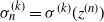 $\sigma_n^{(k)} = \sigma^{(k)}(\boldsymbol{z}^{(n)})$ , for $k = 1,2$ . We are now able to establish our main result.

Theorem 2. (Limit behavior of the number of connected components.) Let us assume that $\kappa_{n} < \infty$ for every $n \in \mathbb{N}$ , that $\kappa_{n} \to \infty$ , and that there exist two sequences $(\varkappa_{n})_{n}$ and $(\varsigma_{n})_n$ such that

\begin{align*} \frac{\kappa_{n}}{\varkappa_{n}} \xrightarrow[n\to\infty]{} 1 \quad \text{and} \quad \frac{\sigma_n^{(2)}}{\varsigma_{n}} \xrightarrow[n\to\infty]{} 1. \end{align*}

In addition, suppose there exists a non-negative constant $\alpha$ such that

(4) \begin{equation} \frac{\big(\sigma_n^{(1)}\big)^2}{\varkappa_{n}\varsigma_{n}} \xrightarrow[n\to\infty]{} \alpha. \end{equation}

Then, for every $[0,c] \subset [0,1[$ , when $n \to \infty$ , the sequence of processes

\begin{align*} \bigg(\frac{1}{\varkappa_{n}}K^{(n)}\bigg(\frac{t}{\varsigma_{n}}\bigg)\bigg)_{t\in[0,c]} \Rightarrow \bigg(1 - t\frac{\alpha}{2}\bigg)_{t\in[0,c]} \quad \text{in } D([0,c], \mathbb{R}) \text{ as } n \to \infty. \end{align*}

In addition, if there exist two non-negative real constants $\beta_1$ and $\beta_2$ such that

(5) \begin{equation} \sqrt{\varkappa_{n}}\bigg(\frac{\kappa_{n}}{\varkappa_{n}} - 1\bigg) \xrightarrow[n\to\infty]{} \beta_1 \quad \text{ and } \quad \sqrt{\varkappa_{n}}\bigg(\frac{(\sigma_n^{(1)})^2}{\varkappa_{n}\varsigma_{n}} - \alpha\bigg) \xrightarrow[n\to\infty]{} \beta_2, \end{equation}

then, when $n \to \infty$ , the sequence of processes

\begin{align*} \bigg(\sqrt{\varkappa_{n}}\bigg(\frac{1}{\varkappa_{n}}K^{(n)}\bigg(\frac{t}{\varsigma_{n}}\bigg) - \bigg(1 - t\frac{\alpha}{2}\bigg)\bigg)\bigg)_{t\in[0,c]} \Rightarrow \bigg(\beta_1 - \beta_2\frac{t}{2} + B\bigg(\alpha\frac t 2\bigg)\bigg)_{t \in [0,c]} \end{align*}

in $D([0,c], \mathbb{R})$ as $n \to \infty$ , and where $(B(t))_{t \ge 0}$ is a Brownian motion.

Remark 3. (On the behavior of (4).) Note that the Cauchy–Schwarz inequality implies that

\begin{align*} \big(\sigma_n^{(1)}\big)^2 = \Bigg(\sum_{i = 1}^{\kappa_{n}}z_i^{(n)}\Bigg)^2 \le \kappa_{n}\sum_{i = 1}^{\kappa_{n}}\big(z_i^{(n)}\big)^2 = \kappa_{n}\sigma_n^{(2)}. \end{align*}

Hence, it is impossible for $(\sigma_n^{(1)})^2 / \kappa_{n} \sigma_n^{(2)}$ (and hence $(\sigma_n^{(1)})^2 / \varkappa_{n} \varsigma_{n}$ ) to diverge to infinity, and there is always at least a convergent sub-sequence. Furthermore, when $\alpha$ as in the statement of Theorem 2 exists, it needs to be an element in [0,1]. However, (5) requires a stronger assumption on the convergence of $(\sigma_n^{(1)})^2 / \varkappa_{n} \varsigma_{n}$ towards $\alpha$ and the speed of convergence being of order $O(1/\sqrt{\varkappa_{n}})$ . Besides, since $\kappa_{n} \to \infty$ , then in order for $\alpha$ to be strictly positive, at least one of the sequences $\sigma_n^{(1)}$ or $\sigma_n^{(2)}$ needs to have an extreme behavior, i.e. $\sigma_n^{(1)} \to \infty$ or $\sigma_n^{(2)} \to 0$ .

The utility of scaling by $\varsigma_{n}$ and $\varkappa_{n}$ instead of $\sigma_n^{(2)}$ and $\kappa_{n}$ may not be immediately clear. However, as shown in the examples explored in Section 3, for certain models it is more natural or informative to use the equivalent $\varsigma_{n}$ and $\varkappa_{n}$ rather than the actual sequences $\sigma_n^{(2)}$ and $\kappa_{n}$ , whose expressions could be more complicated.

Remark 4. (On the functional central limit theorem.) The particular version of the martingale functional central limit theorem that we use in the following is: for each $n \in \mathbb{N}$ , let $M_n$ be a square-integrable local martingale in $D([0,T], \mathbb{R})$ satisfying $M_n(0) = 0$ . Let us assume that the expected maximum jumps of $\langle M_n \rangle$ and $M_n^2$ are asymptotically negligible, i.e. for every $T > 0$ we have $\lim_n \mathbb{E}[J(\langle M_n \rangle , T)] = 0$ and $\lim_n \mathbb{E}[J(M_n , T)^2] = 0$ , where $J(\phi, T)$ is the absolute value of the maximum jump in $\phi \in D([0,T], \mathbb{R})$ over the interval [0, T], i.e. $J(\phi, T) = \sup \{ |\phi(t) - \phi(t\!-\!)| \colon 0 < t \le T \}$ . In addition, there exists a $c > 0$ such that for every $t \ge 0$ we get $\langle M_n \rangle_t \Rightarrow c t $ as $n \to \infty$ , for every $t \in [0,T]$ . Then, $M_n$ converges toward $(B(c t))_{t \in [0,T]}$ when $n \to \infty$ , where B is a Brownian motion.

The statement and proof of this classical result can be found in [Reference Whitt24, Theorem 2.1], cf. [Reference Ethier and Kurtz13, Theorem 1.4, p. 339]. As we commented before, we are able to strengthen the metric of the convergence to the uniform metric because the limit process is continuous.

Proof of Theorem 2. According to Proposition 1, scaling the time by $1/\varsigma_{n}$ and the space by $\varkappa_{n}$ , the process $M^{(n)} = (M^{(n)}(t))_{t \ge 0}$ , where, for every $t \ge 0$ ,

\begin{align*} M^{(n)}(t) = \frac{1}{\varkappa_{n}}K^{(n)}\bigg(\frac{t}{\varsigma_{n}}\bigg) - \frac{\kappa_{n}}{\varkappa_{n}} + \frac{t}{2}\frac{\big(\sigma_n^{(1)}\big)^2}{\varkappa_{n}\varsigma_{n}} - \frac{1}{2\varkappa_{n}\varsigma_{n}}\int_0^t\sum_{i\ge1}\big(X_i^{(n)}\big)^2 \bigg(\frac{s}{\varsigma_{n}}\bigg)\,\mathrm{d}s, \end{align*}

is a local $(\mathcal{G}_t)$ -martingale with predictable quadratic variation

\begin{align*} \langle M^{(n)}\rangle_t = \frac{t}{2}\frac{\big(\sigma_n^{(1)}\big)^2}{(\varkappa_{n})^2\varsigma_{n}} - \frac{1}{2(\varkappa_{n})^2\varsigma_{n}}\int_0^t\sum_{i\ge1}\big(X_i^{(n)}\big)^2 \bigg(\frac{s}{\varsigma_{n}}\bigg)\,\mathrm{d}s, \end{align*}

where $\mathcal{G}_t = \mathcal{F}_{t / \varsigma_{n}}$ for every $t \ge 0$ . Notice that

\begin{align*} \frac{\kappa_{n}}{\varkappa_{n}} \xrightarrow[n\to\infty]{} 1 \quad \text{and} \quad \frac{(\sigma_n^{(1)})^2}{\varkappa_{n}\varsigma_{n}} \xrightarrow[n\to\infty]{} \alpha. \end{align*}

Moreover, we expect the integral term to be negligible, because of Lemma 1. Thus, the limit of $({1}/{\varkappa_{n}})K^{(n)}({t}/{\varsigma_{n}})$ must be $1 - t({\alpha}/{2})$ . Define

\begin{equation*} \Delta^{(n)}(t) \, :\!= \, \frac{1}{\varkappa_{n}}K^{(n)}\bigg(\frac{t}{\varsigma_{n}}\bigg) - \bigg(1 - t\frac{\alpha}{2}\bigg). \end{equation*}

Then $\Delta^{(n)}(t) = M^{(n)}(t) + ({\kappa_{n}}/{\varkappa_{n}}) - 1 + \Theta_1^{(n)}(t) + \Theta_2^{(n)}(t)$ , where

\begin{equation*} \Theta_1^{(n)}(t) = \frac{t}{2}\bigg(\alpha - \frac{\big(\sigma_n^{(1)}\big)^2}{\varkappa_{n}\varsigma_{n}}\bigg) \quad \text{and} \quad \Theta_2^{(n)}(t) = \frac{1}{2\varkappa_{n}\varsigma_{n}} \int_0^t\sum_{i \ge 1}\big(X_i^{(n)}\big)^2\bigg(\frac{s}{\varsigma_{n}}\bigg)\,\mathrm{d}s. \end{equation*}

Now, $\Theta_1^{(n)}$ converges to zero uniformly on [0, c] because of (4). Furthermore, $\Theta_2^{(n)}$ is non-negative and non-decreasing in t, so it suffices to prove the convergence to zero when $t = c$ . Note that, for n large enough that $(c / \varsigma_{n}) \cdot \sigma_n^{(2)} < 1$ , we can use the Fubini–Tonelli theorem, together with Lemma 1, to obtain

(6) \begin{equation} \mathbb{E}\big[\Theta_2^{(n)}(c)\big] \le \frac{1}{2\varkappa_{n}\varsigma_{n}}\int_0^{c} \frac{\sigma_n^{(2)}\,\mathrm{d}s}{1 - (s/\varsigma_{n})\cdot\sigma_n^{(2)}} = -\frac{1}{2\varkappa_{n}}{\ln}\bigg(1 - c\frac{\sigma_n^{(2)}}{\varsigma_{n}}\bigg) \xrightarrow[n\to\infty]{} 0, \end{equation}

which implies the convergence in probability uniformly on [0, c] of $\Theta_2$ to zero, as $n \to \infty$ . Finally, an analogous argument implies that the predictable quadratic variation $\langle M^{(n)}\rangle$ also converges to zero, and then $M^{(n)}$ converges in probability to zero uniformly on [0, c], by using Doob’s maximal inequality or the Burkholder–Davis–Gundy inequality.

Now, to prove the second part of the theorem, note that

\begin{align*} \sqrt{\varkappa_{n}}\Delta^{(n)}(t) = \sqrt{\varkappa_{n}}M^{(n)}(t) + \sqrt{\varkappa_{n}}\bigg(\frac{\kappa_{n}}{\varkappa_{n}} - 1\bigg) + \sqrt{\varkappa_{n}}\Theta_1^{(n)}(t) + \sqrt{\varkappa_{n}}\Theta_2^{(n)}(t). \end{align*}

Because of (5), $t \mapsto \sqrt{\varkappa_{n}}(({\kappa_{n}}/{\varkappa_{n}}) - 1) + \sqrt{\varkappa_{n}}\Theta_1^{(n)}(t)$ , which is a deterministic process and converges towards $t \mapsto \beta_1 - \beta_2t/2$ uniformly on [0, c]. In addition, due to the control of the expectation of $\Theta_2^{(n)}(t)$ established in (6), we also get that $\sqrt{\varkappa_{n}} \Theta_2^{(n)}(c) \to 0$ .

Note that the jumps of $\sqrt{\varkappa_{n}}M^{(n)}$ are given by the jumps of $\sqrt{\varkappa_{n}}K^{(n)}$ , which are all of size $1/\sqrt{\varkappa_{n}}$ and so they converge to zero. Finally, for every $t \in [0,c]$ ,

\begin{align*} \big\langle\sqrt{\varkappa_{n}}M^{(n)}\big\rangle_t = \frac{t}{2}\frac{\big(\sigma_n^{(1)}\big)^2}{\varkappa_{n}\varsigma_{n}} - \frac{1}{2\varkappa_{n}\varsigma_{n}}\int_0^t\sum_{i \ge 1}\big(X_i^{(n)}\big)^2 \bigg(\frac{s}{\varsigma_{n}}\bigg)\,\mathrm{d}s \Rightarrow \frac{t}{2}\alpha \quad \text{as } n \to \infty, \end{align*}

and by using the martingale functional central limit theorem (see Remark 4) we have

\begin{align*} \big(\sqrt{\varkappa_{n}}M^{(n)}(t)\big)_{t\in[0,c]} \Rightarrow \bigg(B\bigg(t\frac{\alpha}{2}\bigg)\bigg)_{t \in [0,c]} \quad \text{as } n \to \infty, \end{align*}

concluding the proof.

In next section we explore the consequences of Theorem 2 for some specific examples of random graph processes.

3. Examples

Theorem 2 is rather general, and it can be applied to several random graph processes. To illustrate this, we now consider, as examples, the Erdős–Rényi random graph (see also Theorem 1 in the introduction), a non-homogeneous version of this model, and a dynamical Norros–Reittu random graph process.

3.1. Erdős–Rényi random graph process

Let us take $\boldsymbol{z}^{(n)}$ to be the vector with n non-null components all equal to one. Then, $\sigma_n^{(1)} = \sigma_n^{(2)} = \kappa_n = n$ . Let us denote by $K_{\mathrm{ER}}^{(n)}$ the process recording the number of connected components in $\mathrm{ER}^{(n)}$ . Then, Theorem 1 in the introduction is immediate from Theorem 2, where $\varsigma_{n} = \varkappa_{n} = n$ , $\alpha = 1$ , and $\beta_1 = \beta_2 = 0$ .

Our method allows us to study more general models. One way to add some non-homogeneity to the Erdős–Rényi random graph model would be to add a unique vertex of mass $\vartheta > 0$ , so that $\boldsymbol{z}^{(n)}$ now consists of n components equal to one, one component equal to $\vartheta$ (located at the beginning or at the end of $\boldsymbol{z}^{(n)}$ depending on whether $\vartheta \ge 1$ or $\vartheta < 1$ ), and infinitely many zeros after. It is easy to see that this perturbed model has the same scaling limit as the Erdős–Rényi graph process. In fact, we could even take $\vartheta_{n}$ depending on n and such that $\vartheta_{n}/ \sqrt{n} \to 0$ , obtaining the same scaling limit again.

Let us then consider a more general model, where the vector of initial masses $\boldsymbol{z}^{(n)}$ satisfies

\begin{align*}\boldsymbol{z}^{(n)} = \mathrm{ord} \Bigg( (\underbrace{1, 1, \dots, 1}_{n \text{ times}}, \vartheta_1, \vartheta_2, \dots, \vartheta_{m_n}, 0, 0, \dots) \Bigg),\end{align*}

and where $\mathrm{ord}\colon l^2 \to l^2_\searrow$ is the natural projection of $l^2$ onto $l^2_\searrow$ . In words, $\boldsymbol{z}^{(n)}$ consists of n elements equal to 1, $m_n$ elements respectively equal to $\vartheta_i$ for $i \in \{1, 2, \dots, m_n\}$ , and infinitely many zeros after. Let us denote by $K_{\mathrm{gER}}^{(n)}$ the process recording the number of connected components in this random graph model.

Corollary 1. (Generalized Erdős-Rényi random graph.) Assume there exist two non-negative constants $\beta_1$ and $\beta_2$ such that

(7) \begin{equation} \frac{m_n}{\sqrt{n}\,} \xrightarrow[n\to\infty]{} \beta_1, \qquad \frac{2}{\sqrt{n}\,}\sum_{i = 1}^{m_n}\vartheta_i \xrightarrow[n\to\infty]{} \beta_2, \qquad \frac{1}{n}\sum_{i = 1}^{m_n}\vartheta_i^2 \xrightarrow[n\to\infty]{} 0. \end{equation}

Then, for every [0, c] with $c < 1$ we have that as $n \to \infty$ the sequence of processes

\begin{align*} \bigg(\frac{1}{n}K_{\mathrm{gER}}^{(n)}\bigg(\frac{t}{n}\bigg)\bigg)_{t \in [0,c]} \Rightarrow \bigg(1 - \frac{t}{2}\bigg)_{t \in [0,c]} \quad \text{in } D([0,c], \mathbb{R}) \text{ as } n \to \infty. \end{align*}

In addition, the sequence of processes

\begin{align*} \bigg(\sqrt{n}\bigg(\frac{1}{n}K_{\mathrm{gER}}^{(n)}\bigg(\frac{t}{n}\bigg) - \bigg(1 - \frac{t}{2}\bigg)\bigg)\bigg)_{t \in [0,c]} \Rightarrow \bigg(\beta_1 - \beta_2t + B\bigg(\frac t 2\bigg)\bigg)_{t \in [0,c]} \end{align*}

in $D([0,c], \mathbb{R})$ as $n \to \infty$ , where B is a Brownian motion.

Remark 5. Notice that (7) can be always satisfied by taking, for instance, $m_n = \lfloor\beta_1\sqrt{n}\rfloor$ and $\vartheta_i = {\beta_2}/{\beta_1}$ for every $i \ge 1$ .

Proof. Notice that

\begin{align*} \frac{\sigma^{(2)}(\boldsymbol{z}^{(n)})}{n} = 1 + \frac{1}{n}\sum_{i = 1}^{m_n}\vartheta_i^2 \xrightarrow[n\to\infty]{} 1 \quad \text{and} \quad \frac{\kappa(\boldsymbol{z}^{(n)})}{n} = 1 + \frac{m_n}{n} \xrightarrow[n\to\infty]{} 1. \end{align*}

In addition,

\begin{align*} \frac{\big(\sigma^{(1)}(\boldsymbol{z}^{(n)})\big)^2}{n^2} = \frac{1}{n^2}\Bigg(n + \sum_{i = 1}^{m_n}\vartheta_i\Bigg)^2 \xrightarrow[n\to\infty]{} 1. \end{align*}

Hence, taking $\varsigma_{n} = \varkappa_{n} = n$ in Theorem 2 we immediately get the first part of the result. To prove the second part, it suffices to notice that

\begin{align*} \sqrt{n}\bigg(\frac{n + m_n}{n} - 1\bigg) & = \frac{m_n}{\sqrt{n}\,} \xrightarrow[n\to\infty]{} \beta_1, \\[3pt] \sqrt{n}\Bigg(\frac{1}{n^2}\Bigg(n + \sum_{i = 1}^{m_n}\vartheta_i\Bigg)^2 - 1\Bigg) & = \frac{2}{\sqrt{n}\,}\sum_{i = 1}^{m_n}\vartheta_i + \frac{1}{\sqrt{n}\,}\Bigg(\frac{1}{\sqrt{n}\,}\sum_{i = 1}^{m_n}\vartheta_i\Bigg)^2 \xrightarrow[n\to\infty]{} \beta_2. \\[-35pt] \end{align*}

3.2. A Norros–Reittu random graph process

Here we consider a version of the multiplicative random graph process, where the weight of each vertex is given by the quantile of a given cumulative distribution function. Notice that this is not the original discrete-time multi-graph model introduced by Norros and Reittu [Reference Norros and Reittu21], which also allows for immigration of vertices and deletion of edges, cf. [Reference van der Hofstad15, Section 6.8.2].

Let F be a cumulative distribution function of a non-negative random variable W, with finite first and second moments. Let us take $w_i^{(n)} \, :\!= \, F^{-1}(1 - (i/n))$ for $i \in [n]$ , where $F^{-1}$ is the generalized inverse of F, i.e. $F^{-1}(x) \, :\!= \, \inf\{s\in\mathbb{R}_+\colon F(s)\ge x\}$ , and where we set $F^{-1}(0) = 0$ . Let also define $z_i^{(n)} \, :\!= \, {w_i^{(n)}}/{\sqrt{l_n}}$ , where $l_n = \sum_{i \ge 1} w_i^{(n)}$ . Thus, it is clear that $\kappa(\boldsymbol{z}^{(n)}) = n$ and

\begin{align*} \frac{\sigma_n^{(1)}}{\sqrt{n}\,} & = \frac{\sigma^{(1)}(\boldsymbol{z}^{(n)})}{\sqrt{n}} = \Bigg(\frac{1}{n}\sum_{i = 1}^n w_i^{(n)}\Bigg)^{1/2} \xrightarrow[n\to\infty]{} \sqrt{\mathbb{E}[W]}, \\[3pt] \sigma_n^{(2)} & = \sigma^{(2)}(\boldsymbol{z}^{(n)}) = \frac{1}{l_n}\sum_{i = 1}^n\big(w_i^{(n)}\big)^2 \xrightarrow[n\to\infty]{} \frac{\mathbb{E}[W^2]}{\mathbb{E}[W]}.\end{align*}

The previous two statements are a consequence of the next elementary lemma, whose proof, for the sake of completeness, is provided in Appendix A.

Lemma 2. (Riemann sum of improper integrals.) Let $\phi\colon (0,1] \to \mathbb{R}_+$ be a non-increasing function such that $\int_0^1\phi(x)\,\mathrm{d}x$ is finite. Then

\begin{align*} \lim_n\frac{1}{n}\sum_{k = 1}^n\phi\bigg(\frac{k}{n}\bigg) = \int_0^1\phi(x)\,\mathrm{d}x. \end{align*}

Furthermore, if $\int_0^1\phi(x)^2\,\mathrm{d}x$ is also finite we get

\begin{align*} \lim_n\sqrt{n}\Bigg(\int_0^1\phi(x)\,\mathrm{d}x - \frac{1}{n}\sum_{k = 1}^n\phi\bigg(\frac{k}{n}\bigg)\Bigg) = 0. \end{align*}

Indeed, it suffices to take $\phi$ in Lemma 2 as $x \mapsto F^{-1}(1 - x)$ and $x \mapsto F^{-1}(1 - x)^2$ . Then, for a uniform on (0, 1) random variable denoted U, $F^{-1}(1-U)$ has distribution function F. Hence, we obtain $\int_0^1F^{-1}(1 - x)^k\,\mathrm{d}x = \mathbb{E}[(F^{-1}(1 - U))^k] = \mathbb{E}[W^k]$ .

Let us denote by $K_{\mathrm{NR}}^{(n)}$ the process recording the number of connected components in this random graph model starting with $\boldsymbol{z}^{(n)}$ as the initial vector of vertex sizes.

Corollary 2. (Norros--Reittu random graph process.) For every $[0,c] \subset [0, {\mathbb{E}[W]}/{\mathbb{E}[W^2]})$ we have that the sequence of processes

\begin{align*} \bigg(\frac{1}{n}K_{\mathrm{NR}}^{(n)}(t)\bigg)_{t \in [0,c]} \Rightarrow \bigg(1 - \frac{t}{2}\mathbb{E}[W]\bigg)_{t \in [0,c]} \quad \textit{in } D([0,c], \mathbb{R}) \text{ as } n \to \infty. \end{align*}

In addition, the sequence of processes of fluctuations

\begin{align*} \bigg(\sqrt{n}\bigg(\frac{1}{n}K_{\mathrm{NR}}^{(n)}(t) - \bigg(1 - \frac{t}{2}\mathbb{E}[W]\bigg)\bigg)\bigg)_{t \in [0,c]} \Rightarrow \bigg(B\bigg(\frac{t\mathbb{E}[W]}{2}\bigg)\bigg)_{t \in [0,c]} \end{align*}

in $D([0,c], \mathbb{R})$ as $n \to \infty$ , where B is a Brownian motion.

Proof. Notice that $\sigma_n^{(2)} \xrightarrow[n\to\infty]{} \varsigma = {\mathbb{E}[W^2]}/{\mathbb{E}[W]}$ . Moreover,

\begin{align*} \frac{\big(\sigma_n^{(1)}\big)^2}{\varsigma n} = \frac{1}{\varsigma n}\sum_{i = 1}^nw_i^{(n)} \xrightarrow[n\to\infty]{} \frac{\mathbb{E}[W]}{\varsigma} = \frac{(\mathbb{E}[W])^2}{\mathbb{E}[W^2]}. \end{align*}

Hence, applying Theorem 2, for every $[0,c] \subset [0,1]$ the sequence of processes

\begin{align*} \bigg(\frac{1}{n}K_{\mathrm{NR}}^{(n)}\bigg(\frac{t}{\varsigma}\bigg)\bigg)_{t \in [0,c]} \Rightarrow \bigg(1 - \frac{t}{2}\frac{\mathbb{E}[W]}{\varsigma}\bigg)_{t \in [0,c]} \quad \text{in } D([0,c], \mathbb{R}) \text{ as } n \to \infty. \end{align*}

In addition,

\begin{align*} \sqrt{n}\bigg(\frac{1}{\varsigma n}\sum_{i = 1}^nw_i^{(n)} - \frac{\mathbb{E}[W]}{\varsigma}\bigg) = \frac{1}{\varsigma}\cdot\sqrt{n}\Bigg(\frac{1}{n}\sum_{i = 1}^nw_i^{(n)} - \mathbb{E}[W]\Bigg) \xrightarrow[n\to\infty]{} 0, \end{align*}

because of Lemma 2. Thus, applying the second half of Theorem 2 we have that when $n \to \infty$ , the sequence of processes

\begin{align*} \bigg(\sqrt{n}\bigg(\frac{1}{n}K^{(n)}\bigg(\frac{t}{\varsigma}\bigg) - \bigg(1 - \frac{t}{2}\frac{\mathbb{E}[W]}{\varsigma}\bigg)\bigg)\bigg)_{t \in [0,c]} \Rightarrow \bigg(B\bigg(\frac{\mathbb{E}[W]}{\varsigma}\frac t 2\bigg)\bigg)_{t \in [0,c]} \end{align*}

in $D([0,c], \mathbb{R})$ as $n \to \infty$ . The result, as stated in the Corollary 2, is obtained by the change of variables $s = t / \varsigma$ .