





1. Introduction
The laminar flow over an airfoil is a canonical problem in fluid mechanics due to its role in aerodynamics and status as a prototypical problem for studying wakes. Unsteady perturbations in the wake are of particular interest for several reasons. First, these perturbations are intimately tied to the separation bubble that forms over the suction side of the airfoil, which in turn increases drag (Alam et al. Reference Alam, Zhou, Yang, Guo and Mi2010; Chang et al. Reference Chang, Zhang, He and Zhou2022). Second, unsteady fluctuations can degrade aerodynamic performance in many aircraft flight control scenarios, such as manoeuvres at high angles of attack, landing, takeoff or encountering atmospheric turbulence. Third, wake perturbations significantly contribute to aerodynamic noise, which is a concern for wind turbines (Wagner, Bareiß & Guidati Reference Wagner, Bareiß and Guidati1996; Agrawal et al. Reference Agrawal, Rosenberg and Sharma2015) and rotorcrafts, including drones. In all these scenarios, accurate estimation and effective closed-loop control of wake perturbations are critical to improve engineering performance, i.e. to reduce drag, enhance flight control and mitigate aerodynamic noise.
A dominant feature of the laminar flow over an airfoil is vortex shedding in the wake. Vortices form on each side of the airfoil and shed periodically, creating downstream flow patterns such as the Kármán vortex street. Factors including the shape of the object, the angle of attack, and the Reynolds number influence this vortex shedding. In NACA0012 airfoils at moderate angles of attack (6°–10°), an anticlockwise vortex is generated at the trailing edge, and a clockwise vortex at the front suction side separates and is entrained downstream (Chang et al. Reference Chang, Zhang, He and Zhou2022) – accordingly, both the front section of the suction side and the trailing edge impact vortex shedding. Many studies have been conducted to suppress vortex shedding in the wakes behind cylinders (Jin, Illingworth & Sandberg Reference Jin, Illingworth and Sandberg2020; Déda et al. Reference Déda, Wolf and Dawson2023; Lin & Tsai Reference Lin and Tsai2024) and airfoils (Colonius & Williams Reference Colonius and Williams2011; Broglia et al. Reference Broglia, Choi, Houston, Pasquale and Zanchetta2018).
An accurate estimator is essential for successful closed-loop control (Stengel Reference Stengel1994; Brunton & Noack Reference Brunton and Noack2015). Standard estimation and control methods such as the Kalman filter (Kalman Reference Kalman1960) and the linear-quadratic-Gaussian (LQG) controller have been applied to fluid mechanics problems over the past two decades, e.g. Kalman filter (Rafiee, Wu & Bayen Reference Rafiee, Wu and Bayen2009; Colburn, Cessna & Bewley Reference Colburn, Cessna and Bewley2011; An et al. Reference An, Wiliams, Eldredge and Colonius2021) and LQG control (Bagheri, Brandt & Henningson Reference Bagheri, Brandt and Henningson2009; Fabbiane et al. Reference Fabbiane, Semeraro, Bagheri and Henningson2014, Reference Fabbiane, Simon, Fischer, Grundmann, Bagheri and Henningson2015, Reference Fabbiane, Bagheri and Henningson2017; Sasaki et al. Reference Sasaki, Morra, Fabbiane, Cavalieri, Hanifi and Henningson2018a ). However, these standard methods have two significant limitations when applied to flow-control problems. First, solving the Riccati equations required to obtain the Kalman and LQG gains scales poorly with problem size and becomes computationally expensive, or in some cases prohibitive, for the large systems typically obtained when discretising the Navier–Stokes equations. This issue can be partially mitigated by reducing the size of the system a priori via some model-reduction method (Pasquale et al. Reference Pasquale, Broglia, Choi, Durante and Zanchetta2017; Gomez et al. Reference Gomez, Lagor, Kirk, Lind, Jones and Paley2019), but this potentially degrades the performance of the controller. Second, standard methods model the nonlinear terms of the Navier–Stokes equations as a white noise forcing on the linear dynamics. These terms are not white (Towne, Brès & Lele Reference Towne, Brès and Lele2017; Zare, Jovanović & Georgiou Reference Zare, Jovanović and Georgiou2017; Morra et al. Reference Morra, Nogueira, Cavalieri and Henningson2021), and treating them as such deteriorates estimation and control performance (Martini et al. Reference Martini, Cavalieri, Jordan, Towne and Lesshafft2020; Amaral et al. Reference Amaral, Cavalieri, Martini, Jordan and Towne2021).
In this paper, we use a recently developed class of estimation and control methods based on resolvent analysis (Martini et al. Reference Martini, Cavalieri, Jordan, Towne and Lesshafft2020, Reference Martini, Jung, Cavalieri, Jordan and Towne2022; Towne, Lozano-Durán & Yang Reference Towne, Lozano-Durán and Yang2020). Resolvent analysis, or input–output analysis, is a powerful methodology based on a linear mapping between forcing (input) and response (output) modes, and the gain between them. These modes and gains are obtained from a singular value decomposition of the resolvent operator obtained from the linearised Navier–Stokes equations. Early studies viewed the input as an external forcing on the Navier–Stokes equations linearised about some laminar fixed point (Jovanović & Bamieh Reference Jovanović and Bamieh2005; Sharma et al. Reference Sharma, Limebeer, McKeon and Morrison2006; Sipp et al. Reference Sipp, Marquet, Meliga and Barbagallo2010). McKeon & Sharma (Reference McKeon and Sharma2010) extended resolvent analysis to turbulent flows by interpreting the nonlinear terms from the Navier–Stokes equations as a forcing on the linear dynamics. Towne, Schmidt & Colonius (Reference Towne, Schmidt and Colonius2018) showed that resolvent modes and spectral proper orthogonal decomposition (SPOD) modes are identical when the forcing is white noise, directly linking resolvent modes to coherent structures observed in flow data. However, resolvent analysis poses computational challenges for high-dimensional problems. To address these difficulties, Ribeiro, Yeh & Taira (Reference Ribeiro, Yeh and Taira2020) applied randomised singular value decompoistion (SVD). Martini et al. (Reference Martini, Cavalieri, Jordan, Towne and Lesshafft2020) used a time-stepping approach to obtain the action of the resolvent operator on a specified forcing, eliminating the need to compute the inverse of large matrices. Farghadan et al. (Reference Farghadan, Martini and Towne2023, Reference Farghadan, Jung, Bhagwat and Towne2024) further extended the range of problems amenable to resolvent analysis by combining randomised SVD with an approach to minimise the cost of the time-stepping method and successfully applied the method to several three-dimensional problems.
Resolvent analysis has been extensively used to study the flow over airfoils at different Reynolds numbers and angles of attack. Thomareis & Papadakis (Reference Thomareis and Papadakis2018) investigated the physics of separated and attached flows around a NACA 0012 airfoil at $\textit {Re}_{L_{c}}=50\,000$
and angle of attack
$\textit {Re}_{L_{c}}=50\,000$
and angle of attack $5^{\circ }$
. Symon, Sipp & McKeon (Reference Symon, Sipp and McKeon2019) investigated two angles of attack,
$5^{\circ }$
. Symon, Sipp & McKeon (Reference Symon, Sipp and McKeon2019) investigated two angles of attack, $0^{\circ }$
and
$0^{\circ }$
and $10^{\circ }$
, for a NACA 0018 airfoil and showed that these two cases behave as an oscillator and amplifier, respectively (Huerre & Monkewitz Reference Huerre and Monkewitz1990). Kojima et al. (Reference Kojima, Yeh, Taira and Kameda2020) identified the origin of the two-dimensional transonic buffet over a NACA 0012 airfoil at
$10^{\circ }$
, for a NACA 0018 airfoil and showed that these two cases behave as an oscillator and amplifier, respectively (Huerre & Monkewitz Reference Huerre and Monkewitz1990). Kojima et al. (Reference Kojima, Yeh, Taira and Kameda2020) identified the origin of the two-dimensional transonic buffet over a NACA 0012 airfoil at $\textit {Re}_{L_{c}}=2000$
,
$\textit {Re}_{L_{c}}=2000$
, $Ma_{\infty }=0.85$
and
$Ma_{\infty }=0.85$
and $\alpha =3^{\circ }$
. Marquet et al. (Reference Marquet, Leontini, Zhao and Thompson2022) studied the flow over a NACA 0012 at
$\alpha =3^{\circ }$
. Marquet et al. (Reference Marquet, Leontini, Zhao and Thompson2022) studied the flow over a NACA 0012 at $\textit {Re}_{L_{c}}=5000$
for angles of attack between
$\textit {Re}_{L_{c}}=5000$
for angles of attack between $\alpha =6.5^{\circ }$
and
$\alpha =6.5^{\circ }$
and $9^{\circ }$
using an incompressible Navier–Stokes linear operator with the mean flow obtained from a numerical simulation, which was validated against experimental data.
$9^{\circ }$
using an incompressible Navier–Stokes linear operator with the mean flow obtained from a numerical simulation, which was validated against experimental data.
Motivated by the ability of resolvent modes to efficiently represent coherent structures, Towne et al. (Reference Towne, Lozano-Durán and Yang2020) introduced a resolvent-based method to estimate space–time flow statistics from limited sensor measurements. Martini et al. (Reference Martini, Cavalieri, Jordan, Towne and Lesshafft2020) extended this method to reconstruct the time series of the flow state using limited measurements. Amaral et al. (Reference Amaral, Cavalieri, Martini, Jordan and Towne2021) used this method to estimate the velocity field in a channel flow using pressure and shear-stress measurements at the channel wall. The aforementioned resolvent-based estimators are non-causal, i.e. they use both past and future measurements to determine the current flow state. Martini et al. (Reference Martini, Jung, Cavalieri, Jordan and Towne2022) derived a causal resolvent-based estimator and controller by enforcing causality using a Wiener–Hopf formalism (Noble Reference Noble1958), making them applicable for closed-loop flow control (Jung et al. Reference Jung, Martini, Cavalieri, Jordan, Lesshafft and Towne2020).
The causal resolvent-based estimator and controller reproduce the Kalman filter and LQG controller, respectively, under equivalent assumptions, namely white-noise forcing. However, the resolvent-based estimator and controller have two crucial advantages over these standard methods. First, they can be efficiently computed even for large systems using a time-stepping method similar to that described earlier for computing resolvent modes or via a data-driven approach. This makes the method applicable to the large problems typical of fluid mechanics without the need for detrimental a priori model reduction. Second, the resolvent-based methods can accommodate coloured-in-time forcing to statistically account for the nonlinear terms from the Navier–Stokes equations, improving estimation accuracy and control efficacy. These benefits are discussed in detail by Martini et al. (Reference Martini, Jung, Cavalieri, Jordan and Towne2022).
Roadmap for resolvent-based estimation and control of the laminar flow over an airfoil.

In this paper, we aim to estimate and control unsteady fluctuations in the wake of a two-dimensional NACA 0012 airfoil at $Ma_{\infty } = 0.3$
,
$Ma_{\infty } = 0.3$
, $Re_{L_{c}} = 5000$
and
$Re_{L_{c}} = 5000$
and $\alpha = 6.5^\circ$
using the resolvent-based methods. The overall roadmap of the paper is depicted schematically in figure 1. We begin in
$\alpha = 6.5^\circ$
using the resolvent-based methods. The overall roadmap of the paper is depicted schematically in figure 1. We begin in $\S$
2 by computing the flow using direct numerical simulation (DNS) and validate the simulation against results in the literature. In
$\S$
2 by computing the flow using direct numerical simulation (DNS) and validate the simulation against results in the literature. In $\S$
3, we analyse the global eigenmodes and resolvent modes of the flow to validate the linearised compressible Navier–Stokes operator and highlight the key flow physics. We then introduce the resolvent-based estimation and control methods in
$\S$
3, we analyse the global eigenmodes and resolvent modes of the flow to validate the linearised compressible Navier–Stokes operator and highlight the key flow physics. We then introduce the resolvent-based estimation and control methods in $\S$
4, discuss how the kernels are computed in
$\S$
4, discuss how the kernels are computed in $\S$
5 and detail our implementation of these tools into a computational fluids dynamics (CFD) code in
$\S$
5 and detail our implementation of these tools into a computational fluids dynamics (CFD) code in $\S$
6. The resolvent-based estimator is applied to both the linearised and nonlinear problems for clean and noisy free stream conditions, the latter of which is designed to disrupt the periodic vortex shedding and induce chaotic fluctuations in the wake, in
$\S$
6. The resolvent-based estimator is applied to both the linearised and nonlinear problems for clean and noisy free stream conditions, the latter of which is designed to disrupt the periodic vortex shedding and induce chaotic fluctuations in the wake, in $\S$
7. Following this, we demonstrate the effectiveness of resolvent-based control for the same systems and flow conditions in
$\S$
7. Following this, we demonstrate the effectiveness of resolvent-based control for the same systems and flow conditions in $\S$
8. Finally,
$\S$
8. Finally, $\S$
9 summarises the paper, highlights its novel contributions and discusses future research directions.
$\S$
9 summarises the paper, highlights its novel contributions and discusses future research directions.
2. Problem set-up and simulation
We aim to use a resolvent-based approach to estimate and mitigate chaotic velocity fluctuations in a laminar airfoil wake. Following Marquet et al. (Reference Marquet, Leontini, Zhao and Thompson2022), we consider the flow around a NACA0012 airfoil at a low chord-based Reynolds number of $Re_{L_{c}} = 5000$
, Mach number of
$Re_{L_{c}} = 5000$
, Mach number of $Ma_{\infty } = 0.3$
and an angle of attack of
$Ma_{\infty } = 0.3$
and an angle of attack of $\alpha = 6.5^{\circ }$
. We consider two different freestream conditions: (i) a clean free stream with no ambient fluctuations and (ii) a noisy free stream with substantial ambient fluctuations generated by random forcing upstream of the airfoil. The flow falls into a periodic limit cycle due to vortex shedding for the clean free stream; the noisy free stream kicks the flow out of this limit cycle, leading to chaotic fluctuations in the wake – a far more challenging problem for estimation and control.
$\alpha = 6.5^{\circ }$
. We consider two different freestream conditions: (i) a clean free stream with no ambient fluctuations and (ii) a noisy free stream with substantial ambient fluctuations generated by random forcing upstream of the airfoil. The flow falls into a periodic limit cycle due to vortex shedding for the clean free stream; the noisy free stream kicks the flow out of this limit cycle, leading to chaotic fluctuations in the wake – a far more challenging problem for estimation and control.
Direct numerical simulation: (a) the full computational C-shaped grid with a close-up view for the wall and wake regions; (b) a snapshot of the instantaneous streamwise velocity $u_x$
with the red dot indicating the probe location at
$u_x$
with the red dot indicating the probe location at $(x, y) / L_c = (2.1, -0.11)$
for the power spectral density in figure 3; (c) the mean streamwise velocity
$(x, y) / L_c = (2.1, -0.11)$
for the power spectral density in figure 3; (c) the mean streamwise velocity $\bar {u}_x$
; and (d) a snapshot of the instantaneous streamwise velocity fluctuation
$\bar {u}_x$
; and (d) a snapshot of the instantaneous streamwise velocity fluctuation $u_x'$
.
$u_x'$
.

We simulate the flow via a direct numerical simulation (DNS) using the compressible flow solver CharLES (Brès et al. Reference Brès, Ham, Nichols and Lele2017). A C-shape mesh is created using Pointwise, as shown in figure 2(a), where the computational grid near the airfoil is also shown in the red box. The leading edge of the airfoil is located at the origin, $x/L_{c}=y/L_{c}=0$
. The size of the domain in the streamwise and normal direction is
$x/L_{c}=y/L_{c}=0$
. The size of the domain in the streamwise and normal direction is $x/L_{c} \in [-49,50]$
and
$x/L_{c} \in [-49,50]$
and $y/L_{c} \in [-50,50]$
, respectively. To create a two-dimensional simulation, the spanwise direction is one cell thick (
$y/L_{c} \in [-50,50]$
, respectively. To create a two-dimensional simulation, the spanwise direction is one cell thick ( $z/L_c \in [0, 0.1]$
) with symmetry boundary conditions. The grid consists of approximately 148 000 cells, with a finer grid resolution applied in the wake region, as studied in Appendix B. Characteristic far-field boundary conditions are applied along the outer boundary of the domain, and a sponge layer is used in the region
$z/L_c \in [0, 0.1]$
) with symmetry boundary conditions. The grid consists of approximately 148 000 cells, with a finer grid resolution applied in the wake region, as studied in Appendix B. Characteristic far-field boundary conditions are applied along the outer boundary of the domain, and a sponge layer is used in the region $x/L_{c}\in [30,50]$
to prevent reflections and ensure an effective outflow boundary condition as the wake exits the domain. Time integration is performed using a third-order total-variation-diminishing Runge–Kutta scheme (Gottlieb & Shu Reference Gottlieb and Shu1998). A constant time step is maintained by setting the Courant–Friedrichs–Lewy (CFL) number to approximately 1. After passing initial transients, data are collected for the duration
$x/L_{c}\in [30,50]$
to prevent reflections and ensure an effective outflow boundary condition as the wake exits the domain. Time integration is performed using a third-order total-variation-diminishing Runge–Kutta scheme (Gottlieb & Shu Reference Gottlieb and Shu1998). A constant time step is maintained by setting the Courant–Friedrichs–Lewy (CFL) number to approximately 1. After passing initial transients, data are collected for the duration $t U_{\infty } / L_c \in [0, 350]$
. This extended time window ensures convergence of the mean and the second-order space–time statistics of vortex shedding in the wake. To verify statistical convergence, we analysed an extended time window
$t U_{\infty } / L_c \in [0, 350]$
. This extended time window ensures convergence of the mean and the second-order space–time statistics of vortex shedding in the wake. To verify statistical convergence, we analysed an extended time window $t U_{\infty } / L_c \in [0, 1000]$
and observed no change.
$t U_{\infty } / L_c \in [0, 1000]$
and observed no change.
Figure 2(b) shows an instantaneous snapshot of the streamwise velocity field around the airfoil. A separation bubble on the suction side of the airfoil and vortex shedding in the wake are clearly observed. The mean streamwise velocity is shown in figure 2(c). The small spatial oscillation observed in the mean wake is likely a consequence of the top-bottom asymmetry of the instantaneous vortex shedding observed in figure 2(b). This mean flow (along with the mean of the other state variables) is used to define the linearisation used to construct the estimation and control kernels. Figure 2(d) shows an instantaneous snapshot of the streamwise velocity fluctuation, i.e. the mean-subtracted velocity. We aim to estimate and control (suppress) such fluctuations.
We validate the DNS via comparisons of the aerodynamic forces and vortex-shedding frequency against the results of Marquet et al. (Reference Marquet, Leontini, Zhao and Thompson2022), who considered incompressible flow over the same airfoil at the same Reynolds number and angle of attack. The time-averaged drag and lift coefficients,
 \begin{equation} C_{D}=\frac {F_{D}}{\frac {1}{2} \rho _{\infty } U_{\infty }^{2} A},\quad C_{L}=\frac {F_{L}}{\frac {1}{2} \rho _{\infty } U_{\infty }^{2} A}, \end{equation}
are reported in table 1. Our results match those of Marquet et al. (Reference Marquet, Leontini, Zhao and Thompson2022) within a 2 % error. The power spectral density (PSD) of the transverse velocity at $x/L_{c}=2.1,y/L_{c}=-0.11$
is shown in figure 3. The vortex-shedding frequency
$x/L_{c}=2.1,y/L_{c}=-0.11$
is shown in figure 3. The vortex-shedding frequency $St_{\alpha } \equiv \omega _{r}(L_{c} {\rm sin}\alpha )/(2 \pi Ma_{\infty })$
is approximately 0.169 in the present study, close to the value of 0.18 found by Marquet et al. (Reference Marquet, Leontini, Zhao and Thompson2022). This slight difference in the aerodynamic forces and vortex-shedding frequency could result from minor differences between the incompressible and compressible flows or differences in the grid refinement (the present grid is more finely resolved).
$St_{\alpha } \equiv \omega _{r}(L_{c} {\rm sin}\alpha )/(2 \pi Ma_{\infty })$
is approximately 0.169 in the present study, close to the value of 0.18 found by Marquet et al. (Reference Marquet, Leontini, Zhao and Thompson2022). This slight difference in the aerodynamic forces and vortex-shedding frequency could result from minor differences between the incompressible and compressible flows or differences in the grid refinement (the present grid is more finely resolved).
Comparison of the time-averaged drag and lift coefficients at $\alpha = 6.5{^\circ }$
with the results from incompressible periodic solution for a NACA 0012 airfoil at
$\alpha = 6.5{^\circ }$
with the results from incompressible periodic solution for a NACA 0012 airfoil at $\textit {Re}_{L_{c}} = 5000$
and
$\textit {Re}_{L_{c}} = 5000$
and $Ma_{\infty } =0.3$
.
$Ma_{\infty } =0.3$
.

PSD of the wall-normal velocity at $(x,y)/L_{c}=(2.1,-0.11)$
.
$(x,y)/L_{c}=(2.1,-0.11)$
.

3. Global stability and resolvent analyses
3.1. Linearisation and global stability analysis
We start with the compressible Navier–Stokes equations written as
 \begin{equation} \frac {\partial \boldsymbol{q}}{\partial t}= \mathcal{F} (\boldsymbol{q}), \end{equation}
where $\boldsymbol{q}$
is a state vector of flow variables
$\boldsymbol{q}$
is a state vector of flow variables $[\rho ,\rho u_{x},\rho u_{y},\rho u_{z},\rho E]^{\rm T}$
and
$[\rho ,\rho u_{x},\rho u_{y},\rho u_{z},\rho E]^{\rm T}$
and $\mathcal{F}$
is the nonlinear Navier–Stokes operator. We linearise about the mean flow rather than a steady fixed point due to the superior ability of the linear operator obtained from the mean flow to model the vortex-shedding frequency and corresponding flow structures observed in data (Barkley Reference Barkley2006; Colonius & Towne Reference Colonius and Towne2025). The equations are linearised using a Reynolds decomposition, giving
$\mathcal{F}$
is the nonlinear Navier–Stokes operator. We linearise about the mean flow rather than a steady fixed point due to the superior ability of the linear operator obtained from the mean flow to model the vortex-shedding frequency and corresponding flow structures observed in data (Barkley Reference Barkley2006; Colonius & Towne Reference Colonius and Towne2025). The equations are linearised using a Reynolds decomposition, giving
 \begin{equation} \frac {\partial \boldsymbol{q}'}{\partial t}-\unicode{x1D63C}\boldsymbol{q}'=\unicode{x1D63D}\boldsymbol{f}(\boldsymbol{\bar {q}},\boldsymbol{q}'), \end{equation}
where $\bar {\boldsymbol{q}}$
and
$\bar {\boldsymbol{q}}$
and $\boldsymbol{q}'$
represent the mean and perturbation state vectors, respectively,
$\boldsymbol{q}'$
represent the mean and perturbation state vectors, respectively, $\unicode{x1D63C} = {\partial \mathcal{F} (\boldsymbol{\bar {q}})}/{\partial \boldsymbol{q}}$
is the linearised Navier–Stokes operator,
$\unicode{x1D63C} = {\partial \mathcal{F} (\boldsymbol{\bar {q}})}/{\partial \boldsymbol{q}}$
is the linearised Navier–Stokes operator, $\boldsymbol{f}$
comprises the remaining nonlinear terms and any exogenous forcing, and
$\boldsymbol{f}$
comprises the remaining nonlinear terms and any exogenous forcing, and $\unicode{x1D63D}$
is an input matrix that can be used to restrict the form of
$\unicode{x1D63D}$
is an input matrix that can be used to restrict the form of $\boldsymbol{f}$
. For convenience, we omit
$\boldsymbol{f}$
. For convenience, we omit $(\cdot )^{\prime }$
for perturbation from this point on. Our approach for constructing
$(\cdot )^{\prime }$
for perturbation from this point on. Our approach for constructing $\unicode{x1D63C}$
is detailed in
$\unicode{x1D63C}$
is detailed in $\S$
6.
$\S$
6.
Eigenspectrum: (a) eigenspectrum, the dotted circle shows the dominant wake eigenmode at the vortex-shedding frequency $St_{\alpha }\approx 0.17$
; (b) the corresponding streamwise velocity eigenmode; and (c) cross-streamwise velocity eigenmode.
$St_{\alpha }\approx 0.17$
; (b) the corresponding streamwise velocity eigenmode; and (c) cross-streamwise velocity eigenmode.

Resolvent-based estimation and control are nominally applicable and robust only for globally stable systems (Schmid & Sipp Reference Schmid and Sipp2016; Martini et al. Reference Martini, Cavalieri, Jordan, Towne and Lesshafft2020, Reference Martini, Jung, Cavalieri, Jordan and Towne2022). Thus, we first conduct a global stability analysis to ensure that our linear operator is stable. Figure 4(a) shows the spectrum of the linearised Navier–Stokes operator $\unicode{x1D63C}$
, represented in terms of the complex frequency
$\unicode{x1D63C}$
, represented in terms of the complex frequency $\omega = i \lambda$
, where
$\omega = i \lambda$
, where $\lambda$
is the eigenvalue of
$\lambda$
is the eigenvalue of $\unicode{x1D63C}$
. The imaginary part
$\unicode{x1D63C}$
. The imaginary part $\omega _i$
is negative for all eigenvalues, indicating that the flow around the airfoil is globally stable. The least-damped eigenvalue appears at the frequency
$\omega _i$
is negative for all eigenvalues, indicating that the flow around the airfoil is globally stable. The least-damped eigenvalue appears at the frequency $St_{\alpha } \approx 0.169$
, which matches the vortex-shedding frequency observed in the PSD in figure 3. The corresponding eigenmode, shown in figures 4(b) and 4(c), exhibits the expected characteristics of vortex shedding (Noack et al. Reference Noack, Afanasiew, Morzynski, Tadmor and Thiele2003).
$St_{\alpha } \approx 0.169$
, which matches the vortex-shedding frequency observed in the PSD in figure 3. The corresponding eigenmode, shown in figures 4(b) and 4(c), exhibits the expected characteristics of vortex shedding (Noack et al. Reference Noack, Afanasiew, Morzynski, Tadmor and Thiele2003).
3.2. Resolvent analysis
Resolvent analysis is central to our estimation and control methods. Therefore, we compute the leading resolvent modes for the airfoil flow as a preliminary step to validate our implementation and to gain insights into the flow physics and the appropriate sensor and actuator placements. After transforming the linear system (3.2) into the frequency domain and solving for the state, we obtain
 \begin{equation} \boldsymbol{\hat{q}} = \unicode{x1D64D} \unicode{x1D63D} \boldsymbol{\hat{f}}, \end{equation}
where the resolvent operator is defined as $\unicode{x1D64D} = (-i \omega \unicode{x1D644} - \unicode{x1D63C})^{-1}$
. The notation (
$\unicode{x1D64D} = (-i \omega \unicode{x1D644} - \unicode{x1D63C})^{-1}$
. The notation ( $\hat{\cdot }$
) indicates a quantity in the frequency domain throughout this paper.
$\hat{\cdot }$
) indicates a quantity in the frequency domain throughout this paper.
Resolvent analysis seeks input and output modes that maximise the resolvent gain
 \begin{equation} \sigma ^{2} = \frac {\| \hat{\boldsymbol{y}} \|^2}{\| \hat{\boldsymbol{f}} \|^2}, \end{equation}
where $\hat{\boldsymbol{y}} = \unicode{x1D63E}\hat{\boldsymbol{q}}$
is an output of interest extracted from the state by the output matrix
$\hat{\boldsymbol{y}} = \unicode{x1D63E}\hat{\boldsymbol{q}}$
is an output of interest extracted from the state by the output matrix $\unicode{x1D63E}$
. The norm is induced by the inner product
$\unicode{x1D63E}$
. The norm is induced by the inner product $\langle \boldsymbol{q}_{1},\boldsymbol{q}_{2}\rangle = \boldsymbol{q}_{1}^{*} \unicode{x1D652} \boldsymbol{q}_{2}$
, where
$\langle \boldsymbol{q}_{1},\boldsymbol{q}_{2}\rangle = \boldsymbol{q}_{1}^{*} \unicode{x1D652} \boldsymbol{q}_{2}$
, where $\unicode{x1D652}$
is a weight matrix used to set a desired norm and
$\unicode{x1D652}$
is a weight matrix used to set a desired norm and $(\cdot )^{*}$
indicates the conjugate transpose. We use the Chu compressible energy norm (Chu Reference Chu1965), and set
$(\cdot )^{*}$
indicates the conjugate transpose. We use the Chu compressible energy norm (Chu Reference Chu1965), and set $\unicode{x1D63D}$
and
$\unicode{x1D63D}$
and $\unicode{x1D63E}$
to the identity matrix for the preliminary resolvent analysis in this section (non-identity values will be used later for estimation and control).
$\unicode{x1D63E}$
to the identity matrix for the preliminary resolvent analysis in this section (non-identity values will be used later for estimation and control).
After defining the weighted resolvent operator
 \begin{equation} {\skew2\tilde {\unicode{x1D64D}}}= \unicode{x1D652}^{\,\frac {1}{2}} \unicode{x1D63E}\unicode{x1D64D} \unicode{x1D63D} \unicode{x1D652}^{\,-\frac {1}{2}}, \end{equation}
the resolvent gains and modes are obtained from the SVD
 \begin{equation} {\skew2\tilde {\unicode{x1D64D}}}=\tilde {\boldsymbol{U}} \Sigma \tilde {\boldsymbol{V}}^{*}. \end{equation}
The resolvent gains are contained within the diagonal matrix $\Sigma = \rm diag[\sigma _{1},\sigma _{2},\ldots,\sigma _{\textit{n}}]$
. The forcing and response modes that maximise (3.4) are recovered as
$\Sigma = \rm diag[\sigma _{1},\sigma _{2},\ldots,\sigma _{\textit{n}}]$
. The forcing and response modes that maximise (3.4) are recovered as $\boldsymbol{V}=\unicode{x1D652}^{\,-{1}/{2}}\tilde {\boldsymbol{V}}$
and
$\boldsymbol{V}=\unicode{x1D652}^{\,-{1}/{2}}\tilde {\boldsymbol{V}}$
and $\boldsymbol{U}=\unicode{x1D652}^{\,-{1}/{2}}\tilde {\boldsymbol{U}}$
, respectively (Towne et al. Reference Towne, Schmidt and Colonius2018). We compute the resolvent modes by transforming the SVD into an equivalent eigenvalue problem, which is solved using an Arnoldi iteration in which the action of
$\boldsymbol{U}=\unicode{x1D652}^{\,-{1}/{2}}\tilde {\boldsymbol{U}}$
, respectively (Towne et al. Reference Towne, Schmidt and Colonius2018). We compute the resolvent modes by transforming the SVD into an equivalent eigenvalue problem, which is solved using an Arnoldi iteration in which the action of $\tilde {\unicode{x1D64D}}$
is obtained by computing its LU decomposition (Jeun, Nichols & Jovanović Reference Jeun, Nichols and Jovanović2016; Schmidt et al. Reference Schmidt, Towne, Rigas, Colonius and Brès2018).
$\tilde {\unicode{x1D64D}}$
is obtained by computing its LU decomposition (Jeun, Nichols & Jovanović Reference Jeun, Nichols and Jovanović2016; Schmidt et al. Reference Schmidt, Towne, Rigas, Colonius and Brès2018).
In figure 5, the peak of the leading resolvent gain is observed at the vortex-shedding frequency $St_{\alpha } \approx 0.169$
. The streamwise and transverse velocity components of the optimal forcing and response modes are shown in figure 5(b–e). The optimal forcing mode is primarily located upstream and above the airfoil, while the optimal response mode is clearly observed downstream in the wake, as expected for a convective flow. The optimal response mode is similar to the dominant eigenmode.
$St_{\alpha } \approx 0.169$
. The streamwise and transverse velocity components of the optimal forcing and response modes are shown in figure 5(b–e). The optimal forcing mode is primarily located upstream and above the airfoil, while the optimal response mode is clearly observed downstream in the wake, as expected for a convective flow. The optimal response mode is similar to the dominant eigenmode.
Resolvent gains, optimal forcing and response modes: (a) leading and second optimal gains; (b) optimal forcing mode of $u_{x}$
; (c) optimal forcing mode of
$u_{x}$
; (c) optimal forcing mode of $ u_{y}$
; (d) optimal response mode of
$ u_{y}$
; (d) optimal response mode of $u_{x}$
; and (e) optimal response mode of
$u_{x}$
; and (e) optimal response mode of $u_{y}$
.
$u_{y}$
.

Block diagram representation of the linear system.

4. Resolvent-based estimation and control framework
In this section, we provide a brief overview of the resolvent-based estimation and control framework developed by Towne et al. (Reference Towne, Lozano-Durán and Yang2020) and Martini et al. (Reference Martini, Cavalieri, Jordan, Towne and Lesshafft2020, Reference Martini, Jung, Cavalieri, Jordan and Towne2022).
4.1. System set-up
As a generalisation of (3.2), we consider the linear time-invariant system
 \begin{align} \frac {{\rm d}\boldsymbol{q}}{{\rm d}t}(t)&= \unicode{x1D63C}\boldsymbol{q}(t)+\unicode{x1D63D}_{f}\boldsymbol{f}(t)+\unicode{x1D63D}_{a}\boldsymbol{a}(t), \end{align}
 \begin{align} \boldsymbol{y}(t)&= \unicode{x1D63E}_{y}\boldsymbol{q}(t)+\boldsymbol{n}(t), \end{align}
 \begin{align} \boldsymbol{z}(t)&= \unicode{x1D63E}_{z}\boldsymbol{q}(t). \end{align}
The system matrix $\unicode{x1D63C} \in \mathbb{C}^{n \times n}$
is the linearised compressible Navier–Stokes operator,
$\unicode{x1D63C} \in \mathbb{C}^{n \times n}$
is the linearised compressible Navier–Stokes operator, $\boldsymbol{q} \in \mathbb{C}^{n}$
is the full state of flow and
$\boldsymbol{q} \in \mathbb{C}^{n}$
is the full state of flow and $n$
is the total size of the state. The forcing
$n$
is the total size of the state. The forcing $\boldsymbol{f} \in \mathbb{C}^{n_{f}}$
represents the nonlinear terms from the Navier–Stokes equations and any exogenous forcing. The forcing matrix
$\boldsymbol{f} \in \mathbb{C}^{n_{f}}$
represents the nonlinear terms from the Navier–Stokes equations and any exogenous forcing. The forcing matrix $\unicode{x1D63D}_{f} \in \mathbb{C}^{n \times n_f}$
restricts the form of the forcing
$\unicode{x1D63D}_{f} \in \mathbb{C}^{n \times n_f}$
restricts the form of the forcing $\boldsymbol{f}$
, e.g. localises it to a certain spatial region. The actuation signal
$\boldsymbol{f}$
, e.g. localises it to a certain spatial region. The actuation signal $\boldsymbol{a} \in \mathbb{C}^{n_{a}}$
, which will be the output of the controller, is mapped onto the system by the actuation matrix
$\boldsymbol{a} \in \mathbb{C}^{n_{a}}$
, which will be the output of the controller, is mapped onto the system by the actuation matrix $\unicode{x1D63D}_{a} \in \mathbb{C}^{n \times n_a}$
, where
$\unicode{x1D63D}_{a} \in \mathbb{C}^{n \times n_a}$
, where $n_a$
is the total number of actuators. The sensor measurement
$n_a$
is the total number of actuators. The sensor measurement $\boldsymbol{y} \in \mathbb{C}^{n_y}$
is extracted from the state by the measurement matrix
$\boldsymbol{y} \in \mathbb{C}^{n_y}$
is extracted from the state by the measurement matrix $\unicode{x1D63E}_{y} \in \mathbb{C}^{n_y \times n}$
, which defines the sensor locations and types, and
$\unicode{x1D63E}_{y} \in \mathbb{C}^{n_y \times n}$
, which defines the sensor locations and types, and $n_y$
is the total number of sensors. The sensor measurements are corrupted by the sensor noise
$n_y$
is the total number of sensors. The sensor measurements are corrupted by the sensor noise $\boldsymbol{n} \in \mathbb{C}^{n_{y}}$
. The target
$\boldsymbol{n} \in \mathbb{C}^{n_{y}}$
. The target $\boldsymbol{z} \in \mathbb{C}^{n_z}$
, i.e. the quantity that we wish to estimate and control, is extracted from the state by the target matrix
$\boldsymbol{z} \in \mathbb{C}^{n_z}$
, i.e. the quantity that we wish to estimate and control, is extracted from the state by the target matrix $\boldsymbol{{C}}_{z} \in \mathbb{C}^{n_z \times n}$
, where
$\boldsymbol{{C}}_{z} \in \mathbb{C}^{n_z \times n}$
, where $n_z$
is the total number of targets. Analogous to other optimal estimation and control methods, the forcing and noise are described by correlations that are assumed to be known.
$n_z$
is the total number of targets. Analogous to other optimal estimation and control methods, the forcing and noise are described by correlations that are assumed to be known.
Following Martini et al. (Reference Martini, Jung, Cavalieri, Jordan and Towne2022), we split the system (4.1) into two parts: the so-called forcing system that is driven by the forcing $\boldsymbol{f}(t)$
and corrupted by the sensor noise
$\boldsymbol{f}(t)$
and corrupted by the sensor noise $\boldsymbol{n}(t)$
,
$\boldsymbol{n}(t)$
,
 \begin{align} \frac {{\rm d}\boldsymbol{q}_{f}}{{\rm d}t}(t)&= \unicode{x1D63C}\boldsymbol{q}_{f}(t)+\unicode{x1D63D}_{f}\boldsymbol{f}(t), \end{align}
 \begin{align} \boldsymbol{y}_{f}(t)&= \unicode{x1D63E}_{y}\boldsymbol{q}_{f}(t)+\boldsymbol{n}(t), \end{align}
 \begin{align} \boldsymbol{z}_{f}(t)&= \unicode{x1D63E}_{z}\boldsymbol{q}_{f}(t), \end{align}
and the actuation system that is driven only by the actuation signal $\boldsymbol{a}(t)$
,
$\boldsymbol{a}(t)$
,
 \begin{align} \frac {{\rm d}\boldsymbol{q}_{a}}{{\rm d}t}(t)&=\unicode{x1D63C}\boldsymbol{q}_{a}(t)+\unicode{x1D63D}_{a}\boldsymbol{a}(t), \end{align}
 \begin{align} \boldsymbol{y}_{a}(t)&=\unicode{x1D63E}_{y}\boldsymbol{q}_{a}(t), \end{align}
 \begin{align} \boldsymbol{z}_{a}(t)&=\unicode{x1D63E}_{z}\boldsymbol{q}_{a}(t). \end{align}
The state, sensor measurements and targets for the full system are recovered as
 \begin{equation} \boldsymbol{q}=\boldsymbol{q}_{f}+\boldsymbol{q}_{a}, \qquad \boldsymbol{y}=\boldsymbol{y}_{f}+\boldsymbol{y}_{a} \quad \textrm {and} \quad \boldsymbol{z}=\boldsymbol{z}_{f}+\boldsymbol{z}_{a}. \end{equation}
By applying the Fourier transform to (4.2) and (4.3), and using the resolvent operator defined in (3.3), we obtain the frequency-domain representations of sensor measurements and targets of the forcing and actuation systems,
 \begin{align} \boldsymbol{\hat{y}}_{f}&= \unicode{x1D64D}_{yf}\boldsymbol{\hat{f}}+\boldsymbol{\hat{n}}, \end{align}
 \begin{align} \boldsymbol{\hat{z}}_{f}&= \unicode{x1D64D}_{zf}\boldsymbol{\hat{f}}, \end{align}
 \begin{align} \boldsymbol{\hat{y}}_{a}&= \unicode{x1D64D}_{ya}\boldsymbol{\hat{a}}, \end{align}
 \begin{align} \boldsymbol{\hat{z}}_{a}&= \unicode{x1D64D}_{za}\boldsymbol{\hat{a}}. \end{align}
Here, $\unicode{x1D64D}_{yf}=\unicode{x1D63E}_{y}\unicode{x1D64D}\unicode{x1D63D}_{f}$
,
$\unicode{x1D64D}_{yf}=\unicode{x1D63E}_{y}\unicode{x1D64D}\unicode{x1D63D}_{f}$
, $\unicode{x1D64D}_{zf}=\unicode{x1D63E}_{z}\unicode{x1D64D}\unicode{x1D63D}_{f}$
,
$\unicode{x1D64D}_{zf}=\unicode{x1D63E}_{z}\unicode{x1D64D}\unicode{x1D63D}_{f}$
, $\unicode{x1D64D}_{ya}=\unicode{x1D63E}_{y}\unicode{x1D64D}\unicode{x1D63D}_{a}$
and
$\unicode{x1D64D}_{ya}=\unicode{x1D63E}_{y}\unicode{x1D64D}\unicode{x1D63D}_{a}$
and $\unicode{x1D64D}_{za}=\unicode{x1D63E}_{z}\unicode{x1D64D}\unicode{x1D63D}_{a}$
are modified resolvent operators (sometimes called input–output operators) that will appear in the resolvent-based estimation and control kernels.
$\unicode{x1D64D}_{za}=\unicode{x1D63E}_{z}\unicode{x1D64D}\unicode{x1D63D}_{a}$
are modified resolvent operators (sometimes called input–output operators) that will appear in the resolvent-based estimation and control kernels.
4.2. Resolvent-based estimation
The resolvent-based estimates of the target $\tilde {\boldsymbol{z}}$
are obtained via a convolution between the sensor measurements and a kernel. Here, we define three distinct resolvent-based estimation kernels: non-causal, truncated non-causal and causal kernels.
$\tilde {\boldsymbol{z}}$
are obtained via a convolution between the sensor measurements and a kernel. Here, we define three distinct resolvent-based estimation kernels: non-causal, truncated non-causal and causal kernels.
First, we define a non-causal estimator
 \begin{equation} \tilde {\boldsymbol{z}}_{nc}(t)=\int _{-\infty }^{\infty } \unicode{x1D64F}_{nc}(t-\tau ) \ \boldsymbol{y}(\tau ){\rm d}\tau , \end{equation}
where $\unicode{x1D64F}_{nc} \in \mathbb{C}^{n_z \times n_y}$
is a non-causal estimation kernel. The optimal estimation kernel is obtained by minimising a cost function defined as the time-integrated expected value of the estimation error,
$\unicode{x1D64F}_{nc} \in \mathbb{C}^{n_z \times n_y}$
is a non-causal estimation kernel. The optimal estimation kernel is obtained by minimising a cost function defined as the time-integrated expected value of the estimation error,
 \begin{equation} {J}_{nc}=\int _{-\infty }^{\infty } \mathbb{E} \big\{ \boldsymbol{e}(t)^{\dagger } \boldsymbol{e}(t)\big\}{\rm d}t, \end{equation}
where the estimation error $ \boldsymbol{e}(t) = \tilde {\boldsymbol{z}}(t) - \boldsymbol{z}(t)$
is the difference between the estimated and true target,
$ \boldsymbol{e}(t) = \tilde {\boldsymbol{z}}(t) - \boldsymbol{z}(t)$
is the difference between the estimated and true target, $(\cdot )^{\dagger }$
denotes the adjoint operator using a suitable inner product, and
$(\cdot )^{\dagger }$
denotes the adjoint operator using a suitable inner product, and $\mathbb{E} \{ \cdot \}$
is the expectation operator. The cost function
$\mathbb{E} \{ \cdot \}$
is the expectation operator. The cost function $ J_{nc}$
is minimised by setting its derivative with respect to
$ J_{nc}$
is minimised by setting its derivative with respect to $ \unicode{x1D64F}_{nc}$
to zero, yielding the optimal non-causal estimation kernel (Martini et al. Reference Martini, Cavalieri, Jordan, Towne and Lesshafft2020)
$ \unicode{x1D64F}_{nc}$
to zero, yielding the optimal non-causal estimation kernel (Martini et al. Reference Martini, Cavalieri, Jordan, Towne and Lesshafft2020)
 \begin{equation} {\skew5\hat{\unicode{x1D64F}}}_{nc}(\omega )= \unicode{x1D64D}_{zf} {\skew5\hat{\unicode{x1D641}}} \unicode{x1D64D}_{yf}^{\dagger } (\unicode{x1D64D}_{yf} {\skew5\hat{\unicode{x1D641}}} \unicode{x1D64D}_{yf}^{\dagger } + {\skew5\hat{\unicode{x1D649}}})^{-1}, \end{equation}
where ${\skew5\hat{\unicode{x1D641}}} = \mathbb{E} \{ \hat{\boldsymbol{f}} \hat{\boldsymbol{f}}^{\dagger } \}$
and
${\skew5\hat{\unicode{x1D641}}} = \mathbb{E} \{ \hat{\boldsymbol{f}} \hat{\boldsymbol{f}}^{\dagger } \}$
and ${\skew5\hat{\unicode{x1D649}}} = \mathbb{E} \{ \hat{\boldsymbol{n}} \hat{\boldsymbol{n}}^{\dagger } \}$
are the cross-spectral densities (CSDs) of the forcing and sensor noise, respectively. The time-domain estimation kernel
${\skew5\hat{\unicode{x1D649}}} = \mathbb{E} \{ \hat{\boldsymbol{n}} \hat{\boldsymbol{n}}^{\dagger } \}$
are the cross-spectral densities (CSDs) of the forcing and sensor noise, respectively. The time-domain estimation kernel $\unicode{x1D64F}_{nc}$
is obtained by inverse Fourier transforming the frequency domain kernel
$\unicode{x1D64F}_{nc}$
is obtained by inverse Fourier transforming the frequency domain kernel ${\skew2\hat{\unicode{x1D64F}}}_{nc}$
. In general, this kernel will be non-causal, i.e.
${\skew2\hat{\unicode{x1D64F}}}_{nc}$
. In general, this kernel will be non-causal, i.e. $\unicode{x1D64F}_{nc}(\tau )$
will not be strictly zero for
$\unicode{x1D64F}_{nc}(\tau )$
will not be strictly zero for $\tau \lt 0$
, therefore requiring future sensor data,
$\tau \lt 0$
, therefore requiring future sensor data, $\boldsymbol{y}(\tau \gt 0)$
, which is unavailable for real-time applications, to evaluate (4.6).
$\boldsymbol{y}(\tau \gt 0)$
, which is unavailable for real-time applications, to evaluate (4.6).
Second, we define a truncated non-causal estimation kernel as a simple baseline approach to address the aforementioned lack of causality. This is done by simply truncating the integral in (4.6),
 \begin{equation} \tilde {\boldsymbol{z}}_{tnc}(t)=\int _{-\infty }^{0} \unicode{x1D64F}_{tnc}(t-\tau )\boldsymbol{y}(\tau ){\rm d}\tau , \end{equation}
which is equivalent to truncating the non-causal part of the kernel,
 \begin{eqnarray} \unicode{x1D64F}_{tnc}(\tau )= \begin{cases} \unicode{x1D64F}_{nc}(\tau ),& \tau \geqslant 0,\\ 0, & \tau \lt 0. \end{cases} \end{eqnarray}
The downside of this approach is that the ex post facto truncation of the optimal non-causal kernel ruins its optimality.
Third, we define an optimal causal resolvent-based estimation kernel by enforcing causality using the Wiener–Hopf formalism (Martinelli Reference Martinelli2009; Martini et al. Reference Martini, Jung, Cavalieri, Jordan and Towne2022). The causal estimator,
 \begin{equation} \tilde {\boldsymbol{z}}_{c}(t)=\int _{-\infty }^{0} \unicode{x1D64F}_{c}(t-\tau )\boldsymbol{y}(\tau ){\rm d}\tau , \end{equation}
is defined in terms of the causal estimation kernel $\unicode{x1D64F}_{c} \in \mathbb{C}^{n_{z} \times n_{y}}$
. To find the optimal kernel under the constraint of causality, we modify the cost function (4.7) to read
$\unicode{x1D64F}_{c} \in \mathbb{C}^{n_{z} \times n_{y}}$
. To find the optimal kernel under the constraint of causality, we modify the cost function (4.7) to read
 \begin{equation} {J}_{c}=\int _{-\infty }^{\infty } \mathbb{E}\big\{ e(t)^{\dagger } e(t)\big\} + \big(\boldsymbol{\mathsf{\Lambda }}_{-}(t) \unicode{x1D64F}_{c} (t) + \boldsymbol{\mathsf{\Lambda }}_{-}^{\dagger }(t) \unicode{x1D64F}_{c}^{\dagger } (t)\big){\rm d}t, \end{equation}
where $\boldsymbol{\mathsf{\Lambda }}$
is a Lagrange multiplier that is used to force the causal kernel to be zero for the non-causal part (
$\boldsymbol{\mathsf{\Lambda }}$
is a Lagrange multiplier that is used to force the causal kernel to be zero for the non-causal part ( $\tau \lt 0$
). The (
$\tau \lt 0$
). The ( $+$
) and (
$+$
) and ( $-$
) subscripts indicate that the non-causal (
$-$
) subscripts indicate that the non-causal ( $\tau \lt 0$
) and causal (
$\tau \lt 0$
) and causal ( $\tau \gt 0$
) parts, respectively, of a matrix or function are set to zero using a Wiener–Hopf factorisation. An introduction to the Wiener–Hopf method is described in Appendix B. Similar to the derivation of (4.8), we minimise the causal cost function (4.12) by setting its derivative with respect to
$\tau \gt 0$
) parts, respectively, of a matrix or function are set to zero using a Wiener–Hopf factorisation. An introduction to the Wiener–Hopf method is described in Appendix B. Similar to the derivation of (4.8), we minimise the causal cost function (4.12) by setting its derivative with respect to $\unicode{x1D64F}_{c}$
to zero. In doing so, we encounter the Wiener–Hopf problem (B4) with
$\unicode{x1D64F}_{c}$
to zero. In doing so, we encounter the Wiener–Hopf problem (B4) with ${\skew5\hat{\unicode{x1D642}}}=\unicode{x1D64D}_{zf}{\skew5\hat{\unicode{x1D641}}}\unicode{x1D64D}_{yf}^{\dagger }$
and
${\skew5\hat{\unicode{x1D642}}}=\unicode{x1D64D}_{zf}{\skew5\hat{\unicode{x1D641}}}\unicode{x1D64D}_{yf}^{\dagger }$
and ${\skew5\hat{\unicode{x1D643}}}=\unicode{x1D64D}_{yf}{\skew5\hat{\unicode{x1D641}}}\unicode{x1D64D}_{yf}^{\dagger } + {\skew5\hat{\unicode{x1D649}}}$
. Using the solution of this Wiener–Hopf problem given by (B8), the causal estimation kernel (Martini et al. Reference Martini, Jung, Cavalieri, Jordan and Towne2022) is
${\skew5\hat{\unicode{x1D643}}}=\unicode{x1D64D}_{yf}{\skew5\hat{\unicode{x1D641}}}\unicode{x1D64D}_{yf}^{\dagger } + {\skew5\hat{\unicode{x1D649}}}$
. Using the solution of this Wiener–Hopf problem given by (B8), the causal estimation kernel (Martini et al. Reference Martini, Jung, Cavalieri, Jordan and Towne2022) is
 \begin{eqnarray} {\skew2\hat{\unicode{x1D64F}}}_{c}(\omega ) &=& \left [ \unicode{x1D64D}_{zf} {\skew5\hat{\unicode{x1D641}}} \unicode{x1D64D}_{yf}^{\dagger } \left(\unicode{x1D64D}_{yf} {\skew5\hat{\unicode{x1D641}}} \unicode{x1D64D}_{yf}^{\dagger } + {\skew5\hat{\unicode{x1D649}}}\right)^{-1}_{-} \right ]_{+} \big(\unicode{x1D64D}_{yf} {\skew5\hat{\unicode{x1D641}}} \unicode{x1D64D}_{yf}^{\dagger } + {\skew5\hat{\unicode{x1D649}}}\kern2.2pt \big)^{-1}_{+}. \end{eqnarray}
4.3. Resolvent-based control
Analogous to the estimation problem, the actuation signal $\boldsymbol{a}(t)$
that will be used to control the flow is obtained via a convolution between the sensor measurements and a control kernel (also referred to as control law in some studies). Again, we consider non-causal, truncated non-causal and causal variations of the resolvent-based control kernels (Martini et al. Reference Martini, Jung, Cavalieri, Jordan and Towne2022).
$\boldsymbol{a}(t)$
that will be used to control the flow is obtained via a convolution between the sensor measurements and a control kernel (also referred to as control law in some studies). Again, we consider non-causal, truncated non-causal and causal variations of the resolvent-based control kernels (Martini et al. Reference Martini, Jung, Cavalieri, Jordan and Towne2022).
The non-causal controller takes the form
 \begin{equation} \boldsymbol{a}_{nc}(t)=\int _{-\infty }^{\infty } \boldsymbol{\mathsf{\Gamma }}_{nc}(t-\tau )\boldsymbol{y}_{f}(\tau ){\rm d}\tau , \end{equation}
where $\boldsymbol{\mathsf{\Gamma }}_{nc} \in \mathbb{C}^{n_a \times n_y}$
is the non-causal control kernel. The optimal kernel is obtained by minimising the cost function
$\boldsymbol{\mathsf{\Gamma }}_{nc} \in \mathbb{C}^{n_a \times n_y}$
is the non-causal control kernel. The optimal kernel is obtained by minimising the cost function
 \begin{equation} {J}_{nc}=\int _{-\infty }^{\infty } \mathbb{E}\big\{\boldsymbol{z}(t)^{\dagger } \boldsymbol{z}(t) + \boldsymbol{a}(t)^{\dagger } \unicode{x1D64B} \boldsymbol{a}(t)\big\}{\rm d}t, \end{equation}
where $\unicode{x1D64B}$
is a weight matrix that penalises the actuation effort. Minimising this cost function yields the optimal non-causal control kernel
$\unicode{x1D64B}$
is a weight matrix that penalises the actuation effort. Minimising this cost function yields the optimal non-causal control kernel
 \begin{eqnarray} {\skew3\hat{\boldsymbol{\mathsf{\Gamma }}}}_{nc}(\omega ) &=& \big(\unicode{x1D64D}_{za}^{\dagger }\unicode{x1D64D}_{za} + {\hat{\unicode{x1D64B}}}\big)^{-1} \big(\!-\unicode{x1D64D}_{za}^{\dagger }\big) \unicode{x1D64D}_{zf} {\skew5\hat{\unicode{x1D641}}} \unicode{x1D64D}_{yf}^{\dagger } \big(\unicode{x1D64D}_{yf} {\skew5\hat{\unicode{x1D641}}} \unicode{x1D64D}_{yf}^{\dagger } + {\skew5\hat{\unicode{x1D649}}}\big)^{-1}. \end{eqnarray}
The truncated non-causal control kernel is defined as
 \begin{eqnarray} \boldsymbol{\mathsf{\Gamma }}_{tnc}(\tau )= \bigg\{\kern-5pt\begin{array}{ll}\boldsymbol{\mathsf{\Gamma }}_{nc}(\tau ),& \tau \geqslant 0,\\ 0, & \tau \lt 0, \end{array}\end{eqnarray}
from which the actuation signal is computed as
 \begin{equation} \boldsymbol{a}_{tnc}(t)=\int _{-\infty }^{0} \boldsymbol{\mathsf{\Gamma }}_{tnc}(t-\tau )\boldsymbol{y}_{f}(\tau ){\rm d}\tau . \end{equation}
As before, truncating the optimal non-causal kernel yields a non-optimal causal kernel.
Finally, the optimal causal controller is
 \begin{equation} \boldsymbol{a}_{c}(t)=\int _{-\infty }^{0} \boldsymbol{\mathsf{\Gamma }}_{c}(t-\tau )\boldsymbol{y}_{f}(\tau ){\rm d}\tau , \end{equation}
and the optimal causal control kernel is obtained by using Lagrange multipliers to enforce causality, expressed by the cost function
 \begin{equation} {J}_{c}=\int _{-\infty }^{\infty } \mathbb{E}\big\{\boldsymbol{z}(t)^{\dagger } \boldsymbol{z}(t) + \boldsymbol{a}(t)^{\dagger } \unicode{x1D64B} \boldsymbol{a}(t) + (\boldsymbol{\mathsf{\Lambda }}_{-}(t) \boldsymbol{\mathsf{\Gamma }}_{c} (t) + \boldsymbol{\mathsf{\Lambda }}_{-}^{\dagger }(t) \boldsymbol{\mathsf{\Gamma }}_{c}^{\dagger } (t)) \big\}{\rm d}t. \end{equation}
Minimising (4.20) leads to the Wiener–Hopf problem (B5) with ${\skew5\hat{\unicode{x1D646}}}=\unicode{x1D64D}_{za}^{\dagger }\unicode{x1D64D}_{za} + {\hat{\unicode{x1D64B}}}$
and
${\skew5\hat{\unicode{x1D646}}}=\unicode{x1D64D}_{za}^{\dagger }\unicode{x1D64D}_{za} + {\hat{\unicode{x1D64B}}}$
and ${\hat{\unicode{x1D647}}}=-\unicode{x1D64D}_{za}^{\dagger }$
. Using the solution of this Wiener–Hopf problem given in (B9), the optimal causal resolvent-based control kernel is
${\hat{\unicode{x1D647}}}=-\unicode{x1D64D}_{za}^{\dagger }$
. Using the solution of this Wiener–Hopf problem given in (B9), the optimal causal resolvent-based control kernel is
 \begin{eqnarray} {\skew3\hat{\boldsymbol{\mathsf{\Gamma }}}}_{c}(\omega )&=& \big(\unicode{x1D64D}_{za}^{\dagger }\unicode{x1D64D}_{za}+{\hat{\unicode{x1D64B}}}\big)_{+}^{-1}\big[\big(\unicode{x1D64D}_{za}^{\dagger }\unicode{x1D64D}_{za}+{\hat{\unicode{x1D64B}}}\big)_{-}^{-1}\nonumber \big(\kern-2pt-\kern-1pt\unicode{x1D64D}_{za}^{\dagger }\big)\unicode{x1D64D}_{zf}{\skew5\hat{\unicode{x1D641}}}\unicode{x1D64D}_{yf}^{\dagger }\\ &&\big(\unicode{x1D64D}_{yf}{\skew5\hat{\unicode{x1D641}}}\unicode{x1D64D}_{yf}^{\dagger }+ {\skew5\hat{\unicode{x1D649}}}\big)_{-}^{-1}\big]_{+}\big(\unicode{x1D64D}_{yf}{\skew5\hat{\unicode{x1D641}}}\unicode{x1D64D}_{yf}^{\dagger }+ {\skew5\hat{\unicode{x1D649}}}\big)_{+}^{-1}. \end{eqnarray}
In (4.14), (4.18) and (4.19), the actuation signal is obtained as a convolution between the control kernel and the sensor measurement $\boldsymbol{y}_{f}$
for the forcing system (4.2), i.e. the control kernels were derived using a measurement excluding the response of the system (4.3) to actuation. In practice, only the complete measurement
$\boldsymbol{y}_{f}$
for the forcing system (4.2), i.e. the control kernels were derived using a measurement excluding the response of the system (4.3) to actuation. In practice, only the complete measurement $\boldsymbol{y}=\boldsymbol{y}_f + \boldsymbol{y}_a$
is available. Considering the full (combined) linear system (4.1), the final closed-loop controller takes the form
$\boldsymbol{y}=\boldsymbol{y}_f + \boldsymbol{y}_a$
is available. Considering the full (combined) linear system (4.1), the final closed-loop controller takes the form
 \begin{equation} \boldsymbol{a}(t)=\int _{-\infty }^{0} \boldsymbol{\mathsf{\Gamma }}_{cl}(t-\tau )\boldsymbol{y}(\tau ){\rm d}\tau , \end{equation}
where the final closed-loop kernel is
 \begin{eqnarray} {\skew3\hat{\boldsymbol{\mathsf{\Gamma }}}}_{cl} &=& \big(\unicode{x1D644} + {\skew3\hat{\boldsymbol{\mathsf{\Gamma }}}} \unicode{x1D64D}_{ya}\big)^{-1} {\skew3\hat{\boldsymbol{\mathsf{\Gamma }}}}, \end{eqnarray}
with $\hat{\boldsymbol{\mathsf{\Gamma }}}$
replaced by
$\hat{\boldsymbol{\mathsf{\Gamma }}}$
replaced by ${\skew3\hat{\boldsymbol{\mathsf{\Gamma }}}}_{tnc}$
or
${\skew3\hat{\boldsymbol{\mathsf{\Gamma }}}}_{tnc}$
or ${\skew3\hat{\boldsymbol{\mathsf{\Gamma }}}}_{c}$
for truncated non-causal and optimal causal resolvent-based control, respectively.
${\skew3\hat{\boldsymbol{\mathsf{\Gamma }}}}_{c}$
for truncated non-causal and optimal causal resolvent-based control, respectively.
5. Computing estimation and control kernels
In this section, we present two approaches to compute resolvent-based estimation and control kernels (Martini et al. Reference Martini, Jung, Cavalieri, Jordan and Towne2022). First, we describe an operator-based approach that allows for efficient implementation of linear simulations without the need for inverting the operator or performing prior model reduction, making it particularly efficient for large-scale problems. Second, we explain a data-driven approach that does not require the construction of the linearised Navier–Stokes operator. Instead, this method uses training data from simulations or experiments to build cross-spectral densities, which are then used to compute the components of the estimation and control kernels.
5.1. Operator-based approach
The resolvent operator $\unicode{x1D64D}$
is defined in terms of an inverse, the cost of which scales poorly with the problem dimension
$\unicode{x1D64D}$
is defined in terms of an inverse, the cost of which scales poorly with the problem dimension $n$
and becomes computationally expensive for large systems. To circumvent this, we employ a time-stepping approach that avoids the inverse operation and instead constructs the necessary modified resolvent operators that appear in the estimation and control kernels by solving linear equations in the time domain (Martini et al. Reference Martini, Cavalieri, Jordan, Towne and Lesshafft2020, Reference Martini, Jung, Cavalieri, Jordan and Towne2022; Farghadan, Martini & Towne Reference Farghadan, Martini and Towne2023). For both cases, the cost of this approach scales linearly with the problem dimension, avoiding the need to reduce the system via a priori model reduction and the associated loss of accuracy. Individual modified resolvent operators such as
$n$
and becomes computationally expensive for large systems. To circumvent this, we employ a time-stepping approach that avoids the inverse operation and instead constructs the necessary modified resolvent operators that appear in the estimation and control kernels by solving linear equations in the time domain (Martini et al. Reference Martini, Cavalieri, Jordan, Towne and Lesshafft2020, Reference Martini, Jung, Cavalieri, Jordan and Towne2022; Farghadan, Martini & Towne Reference Farghadan, Martini and Towne2023). For both cases, the cost of this approach scales linearly with the problem dimension, avoiding the need to reduce the system via a priori model reduction and the associated loss of accuracy. Individual modified resolvent operators such as $\unicode{x1D64D}_{za}$
and
$\unicode{x1D64D}_{za}$
and $\unicode{x1D64D}_{ya}$
can be obtained using a single-stage run of the direct linear equations. Products of modified resolvent operators (and the forcing CSD) such as
$\unicode{x1D64D}_{ya}$
can be obtained using a single-stage run of the direct linear equations. Products of modified resolvent operators (and the forcing CSD) such as $\unicode{x1D64D}_{zf}{\skew5\hat{\unicode{x1D641}}}\unicode{x1D64D}_{yf}^{\dagger }$
and
$\unicode{x1D64D}_{zf}{\skew5\hat{\unicode{x1D641}}}\unicode{x1D64D}_{yf}^{\dagger }$
and $\unicode{x1D64D}_{yf} {\skew5\hat{\unicode{x1D641}}}\unicode{x1D64D}_{yf}^{\dagger }$
can be obtained with greater efficiently using two-stage runs of both the adjoint and direct linear equations.
$\unicode{x1D64D}_{yf} {\skew5\hat{\unicode{x1D641}}}\unicode{x1D64D}_{yf}^{\dagger }$
can be obtained with greater efficiently using two-stage runs of both the adjoint and direct linear equations.
5.1.1. Single-stage run
The operators $\unicode{x1D64D}_{za}$
and
$\unicode{x1D64D}_{za}$
and $\unicode{x1D64D}_{ya}$
appearing in (4.21) and (4.23), respectively, can be constructed by computing a series of impulse responses of the actuation system (4.3),
$\unicode{x1D64D}_{ya}$
appearing in (4.21) and (4.23), respectively, can be constructed by computing a series of impulse responses of the actuation system (4.3),
 \begin{align} \frac {{\rm d}\boldsymbol{q}_{a,k}}{{\rm d}t}(t) &= \unicode{x1D63C}\boldsymbol{q}_{a,k}(t)+\unicode{x1D63D}_{a,k}\delta (t), \end{align}
 \begin{align} \boldsymbol{y}_{a,k}(t)&= \unicode{x1D63E}_{y}\boldsymbol{q}_{a,k}(t), \end{align}
 \begin{align} \boldsymbol{z}_{a,k}(t)&= \unicode{x1D63E}_{z}\boldsymbol{q}_{a,k}(t). \end{align}
Here, $\boldsymbol{y}_{a,k} \in \mathbb{C}^{n_{y}}$
and
$\boldsymbol{y}_{a,k} \in \mathbb{C}^{n_{y}}$
and $\boldsymbol{z}_{a,k} \in \mathbb{C}^{n_{z}}$
are the sensor and target measurement of the direct system forced by an impulse
$\boldsymbol{z}_{a,k} \in \mathbb{C}^{n_{z}}$
are the sensor and target measurement of the direct system forced by an impulse $\delta (t)$
located at the
$\delta (t)$
located at the $k=1, 2, 3,\dots$
actuator, as encoded by the
$k=1, 2, 3,\dots$
actuator, as encoded by the $k=1, 2, 3,\dots$
column of the actuation matrix,
$k=1, 2, 3,\dots$
column of the actuation matrix, $\unicode{x1D63D}_{a,k}$
. By collecting these data for each actuator
$\unicode{x1D63D}_{a,k}$
. By collecting these data for each actuator $k=1,\dots ,n_a$
and taking a Fourier transform, we obtain
$k=1,\dots ,n_a$
and taking a Fourier transform, we obtain
 \begin{align} {\; \;\hat{\kern-4pt\unicode{x1D654}}}_{a} &= \begin{bmatrix} \hat{\boldsymbol{y}}_{a,1}&\hat{\boldsymbol{y}}_{a,2} & \dots & \hat{\boldsymbol{y}}_{a,n_{a}} \end{bmatrix} = \unicode{x1D64D}_{ya}, \end{align}
 \begin{align} {\; \;\hat{\kern-3.5pt\unicode{x1D655}}}_{a} &= \begin{bmatrix} \hat{\boldsymbol{z}}_{a,1}&\hat{\boldsymbol{z}}_{a,2}& \dots & \hat{\boldsymbol{z}}_{a,n_{a}} \end{bmatrix} = \unicode{x1D64D}_{za}, \end{align}
with ${\; \hat{\kern-4pt\unicode{x1D654}}}_{a} \in \mathbb{C}^{n_{y} \times n_{a}}$
and
${\; \hat{\kern-4pt\unicode{x1D654}}}_{a} \in \mathbb{C}^{n_{y} \times n_{a}}$
and ${ \; \;\hat{\kern-3.5pt\unicode{x1D655}}}_{a} \in \mathbb{C}^{n_{z} \times n_{a}}$
. That is, the Fourier transform of each measurement
${ \; \;\hat{\kern-3.5pt\unicode{x1D655}}}_{a} \in \mathbb{C}^{n_{z} \times n_{a}}$
. That is, the Fourier transform of each measurement $\boldsymbol{y}_{a,k}$
and
$\boldsymbol{y}_{a,k}$
and $\boldsymbol{z}_{a,k}$
yields a column of the modified resolvent operators
$\boldsymbol{z}_{a,k}$
yields a column of the modified resolvent operators $\unicode{x1D64D}_{ya}$
and
$\unicode{x1D64D}_{ya}$
and $\unicode{x1D64D}_{za}$
, respectively.
$\unicode{x1D64D}_{za}$
, respectively.
5.1.2. Two-stage run
While single-stage runs could be used to construct all of the modified resolvent operators in the estimation and control kernels, certain products thereof can be constructed more efficiently using pairs of adjoint and direct runs. The procedure begins with solving the adjoint system
 \begin{align} -\frac {{\rm d}\boldsymbol{q}_{f,i}}{{\rm d}t}(t) &= \unicode{x1D63C}^{\dagger }\boldsymbol{q}_{f,i}(t)+\unicode{x1D63E}_{y,i}^{\dagger }\delta (t), \end{align}
 \begin{align} \boldsymbol{s}_{i}(t)&= \unicode{x1D63D}_{f}^{\dagger }\boldsymbol{q}_{f,i}(t), \end{align}
where $\unicode{x1D63C}^{\dagger }$
is the adjoint linearised Navier–Stokes operator and the subscript
$\unicode{x1D63C}^{\dagger }$
is the adjoint linearised Navier–Stokes operator and the subscript $i$
indicates the sensor defined by the
$i$
indicates the sensor defined by the $i$
th row of the sensor measurement matrix
$i$
th row of the sensor measurement matrix $\unicode{x1D63E}_y$
. The output
$\unicode{x1D63E}_y$
. The output $\boldsymbol{s}_{i}$
of the adjoint run is used as a forcing in a corresponding direct run of the forcing system (4.2),
$\boldsymbol{s}_{i}$
of the adjoint run is used as a forcing in a corresponding direct run of the forcing system (4.2),
 \begin{align} \frac {{\rm d}\boldsymbol{q}_{f,i}}{{\rm d}t}(t) &= \unicode{x1D63C}\boldsymbol{q}_{f,i}(t)+\unicode{x1D63D}_{f}\boldsymbol{s}_{i}(t), \end{align}
 \begin{align} \boldsymbol{y}_{f,i}(t) &= \unicode{x1D63E}_{y}\boldsymbol{q}_{f,i}(t) +\boldsymbol{n}_{i}(t), \end{align}
 \begin{align} \boldsymbol{z}_{f,i}(t) &= \unicode{x1D63E}_{z}\boldsymbol{q}_{f,i}(t). \end{align}
As in the single-stage run, by collecting each of the final sensor and target measurements, and taking a Fourier transform, we obtain
 \begin{align} {\; \;\hat{\kern-4pt\unicode{x1D654}}}_{f} &= \begin{bmatrix} \hat{\boldsymbol{y}}_{1}&\hat{\boldsymbol{y}}_{2} & \dots & \hat{\boldsymbol{y}}_{n_{y}} \end{bmatrix} = \unicode{x1D64D}_{yf}\unicode{x1D64D}_{yf}^{\dagger }, \end{align}
 \begin{align} {\; \;\hat{\kern-3.5pt\unicode{x1D655}}}_{f} &= \begin{bmatrix} \hat{\boldsymbol{z}}_{1}&\,\hat{\boldsymbol{z}}_{2}& \dots &\, \hat{\boldsymbol{z}}_{n_{y}} \end{bmatrix} = \unicode{x1D64D}_{zf} \unicode{x1D64D}_{yf}^{\dagger }, \end{align}
with ${\; \hat{\kern-4pt\unicode{x1D654}}}_{f} \in \mathbb{C}^{n_{y} \times n_{y}}$
and
${\; \hat{\kern-4pt\unicode{x1D654}}}_{f} \in \mathbb{C}^{n_{y} \times n_{y}}$
and ${\; \hat{\kern-3.5pt\unicode{x1D655}}}_{f} \in \mathbb{C}^{n_{z} \times n_{y}}$
. To account for the nonlinearity of the flow, the coloured forcing statistics,
${\; \hat{\kern-3.5pt\unicode{x1D655}}}_{f} \in \mathbb{C}^{n_{z} \times n_{y}}$
. To account for the nonlinearity of the flow, the coloured forcing statistics, $\hat{\unicode{x1D641}}$
, can be incorporated into (5.5) during adjoint and direct simulations, resulting in
$\hat{\unicode{x1D641}}$
, can be incorporated into (5.5) during adjoint and direct simulations, resulting in $\unicode{x1D64D}_{yf} {\skew5\hat{\unicode{x1D641}}} \unicode{x1D64D}_{yf}^{\dagger }$
and
$\unicode{x1D64D}_{yf} {\skew5\hat{\unicode{x1D641}}} \unicode{x1D64D}_{yf}^{\dagger }$
and $\unicode{x1D64D}_{zf} {\skew5\hat{\unicode{x1D641}}} \unicode{x1D64D}_{yf}^{\dagger }$
(Jung Reference Jung2024).
$\unicode{x1D64D}_{zf} {\skew5\hat{\unicode{x1D641}}} \unicode{x1D64D}_{yf}^{\dagger }$
(Jung Reference Jung2024).
Finally, (5.2) and (5.5) are used to write the estimation kernels in (4.8) and (4.13), and control kernels in (4.16) and (4.21) in terms of ${\; \hat{\kern-4pt\unicode{x1D654}}}_{a}$
,
${\; \hat{\kern-4pt\unicode{x1D654}}}_{a}$
, ${\; \hat{\kern-3.5pt\unicode{x1D655}}}_{a}$
,
${\; \hat{\kern-3.5pt\unicode{x1D655}}}_{a}$
, ${\; \hat{\kern-4pt\unicode{x1D654}}}_{f}$
and
${\; \hat{\kern-4pt\unicode{x1D654}}}_{f}$
and ${\; \hat{\kern-3.5pt\unicode{x1D655}}}_{f}$
. The final operator-based estimation and control kernels are
${\; \hat{\kern-3.5pt\unicode{x1D655}}}_{f}$
. The final operator-based estimation and control kernels are
 \begin{align} {\skew2\hat{\unicode{x1D64F}}}_{nc,O} &= {\; \;\hat{\kern-3.5pt\unicode{x1D655}}}_{f} \big( {\; \;\hat{\kern-4pt\unicode{x1D654}}}_{f} + {\skew5\hat{\unicode{x1D649}}}\big)^{-1}, \end{align}
 \begin{align} {\skew2\hat{\unicode{x1D64F}}}_{c,O} &= \big[{\; \;\hat{\kern-3.5pt\unicode{x1D655}}}_{f} \big( {\; \;\hat{\kern-4pt\unicode{x1D654}}}_{f} + {\skew5\hat{\unicode{x1D649}}} \big)^{-1}_{-}\big]_{+} \big({\; \;\hat{\kern-4pt\unicode{x1D654}}}_{f}+ {\skew5\hat{\unicode{x1D649}}}\big)_{+}^{-1}, \end{align}
and
 \begin{align} {\skew3\hat{\boldsymbol{\mathsf{\Gamma }}}}_{nc,O} &= \big(\hat{\boldsymbol{Z}}_{a}^{\dagger } \hat{\boldsymbol{Z}}_{a} +\hat{\boldsymbol{P}}\big)^{-1} \big({-}\hat{\boldsymbol{Z}}_{a}^{\dagger }\big) \hat{\boldsymbol{Z}}_{f} \big(\hat{\boldsymbol{Y}}_{f}+ {\skew5\hat{\unicode{x1D649}}}\big)^{-1}, \end{align}
 \begin{align} {\skew3\hat{\boldsymbol{\mathsf{\Gamma }}}}_{c,O} &= \big({\; \;\hat{\kern-3.5pt\unicode{x1D655}}}_{a}^{\dagger } {\; \;\hat{\kern-3.5pt\unicode{x1D655}}}_{a}+{\hat{\unicode{x1D64B}}}\big)_{+}^{-1}\big[\big({\; \;\hat{\kern-3.5pt\unicode{x1D655}}}_{a}^{\dagger } {\; \;\hat{\kern-3.5pt\unicode{x1D655}}}_{a}+{\hat{\unicode{x1D64B}}}\big)_{-}^{-1} \big({-}{\; \;\hat{\kern-3.5pt\unicode{x1D655}}}_{a}^{\dagger }\big){\; \;\hat{\kern-3.5pt\unicode{x1D655}}}_{f}\big({\; \;\hat{\kern-4pt\unicode{x1D654}}}_{f}+ {\skew5\hat{\unicode{x1D649}}}\big)_{-}^{-1}\big]_{+}\big({\; \;\hat{\kern-4pt\unicode{x1D654}}}_{f}+ {\skew5\hat{\unicode{x1D649}}}\big)_{+}^{-1}. \\[6pt] \nonumber \end{align}
5.2. Data-driven approach
When the linearised Navier–Stokes operator is unavailable, a data-driven approach (Martini et al. Reference Martini, Jung, Cavalieri, Jordan and Towne2022) can be employed to build the required modified resolvent operators using CSDs computed from data (Towne et al. Reference Towne, Schmidt and Colonius2018, Reference Towne, Lozano-Durán and Yang2020). This approach extends the applicability of resolvent-based estimation and control to experimental settings and circumvents the need for adjoint solvers. Additionally, when the CSD is computed from the dataset of a nonlinear system, the resulting kernels automatically include the forcing CSD $\hat{\unicode{x1D641}}$
, which statistically accounts for the nonlinearity of the flow, thereby improving the estimation and control performance for the nonlinear system.
$\hat{\unicode{x1D641}}$
, which statistically accounts for the nonlinearity of the flow, thereby improving the estimation and control performance for the nonlinear system.
The nonlinear terms in the Navier–Stokes equations act as a forcing of the resolvent operator (McKeon & Sharma Reference McKeon and Sharma2010) and their influence is crucial in complex dynamic systems (Amaral et al. Reference Amaral, Cavalieri, Martini, Jordan and Towne2021). To explicitly address the nonlinear terms, we split the forcing vector $\boldsymbol{f}$
into two components: the external forcing
$\boldsymbol{f}$
into two components: the external forcing $\boldsymbol{f}_{\textit{ext}}$
and the nonlinear terms
$\boldsymbol{f}_{\textit{ext}}$
and the nonlinear terms $\boldsymbol{f}_{nl}$
. This distinction helps us better understand their impact when building the CSDs from the data. The overall forcing term in (4.1) can be split as
$\boldsymbol{f}_{nl}$
. This distinction helps us better understand their impact when building the CSDs from the data. The overall forcing term in (4.1) can be split as
 \begin{equation} \unicode{x1D63D}_{f}\boldsymbol{f} \\ = \begin{bmatrix} \unicode{x1D63D}_{\textit{ext}} & \unicode{x1D63D}_{nl} \end{bmatrix} \begin{bmatrix} \boldsymbol{f}_{\textit{ext}} \\ \boldsymbol{f}_{nl} \end{bmatrix}, \end{equation}
where $\unicode{x1D63D}_{\textit{ext}} \in \mathbb{C}^{n \times n_{\textit{ext}}}$
and
$\unicode{x1D63D}_{\textit{ext}} \in \mathbb{C}^{n \times n_{\textit{ext}}}$
and $\unicode{x1D63D}_{nl} \in \mathbb{C}^{n \times n}$
. Typically, the region subject to external forcing is smaller than the overall domain, such that
$\unicode{x1D63D}_{nl} \in \mathbb{C}^{n \times n}$
. Typically, the region subject to external forcing is smaller than the overall domain, such that $n_{\textit{ext}}\lt n$
. In a linear system, the nonlinear terms
$n_{\textit{ext}}\lt n$
. In a linear system, the nonlinear terms $\boldsymbol{f}_{nl}$
are not included, allowing us to analyse the linear dynamics of the flow, and to build linear estimators and controllers. However, our ultimate goal is to manipulate the unsteady fluctuations inherent in the actual flow, which necessitates considering nonlinearity. For the nonlinear system, we collect data from the systems without and with external forcing to better capture the behaviour of the systems influenced by external forcing. The forcing system (4.2) without and with the external forcing can be expressed as
$\boldsymbol{f}_{nl}$
are not included, allowing us to analyse the linear dynamics of the flow, and to build linear estimators and controllers. However, our ultimate goal is to manipulate the unsteady fluctuations inherent in the actual flow, which necessitates considering nonlinearity. For the nonlinear system, we collect data from the systems without and with external forcing to better capture the behaviour of the systems influenced by external forcing. The forcing system (4.2) without and with the external forcing can be expressed as
 \begin{align} \frac {{\rm d}\boldsymbol{q}}{{\rm d}t}(t) & = \unicode{x1D63C}\boldsymbol{q}(t)+\unicode{x1D63D}_{nl}\boldsymbol{f}_{nl}(t),\end{align}
 \begin{align} \frac {{\rm d}\boldsymbol{q}_{e}}{{\rm d}t}(t)& = \unicode{x1D63C}\boldsymbol{q}_{e}(t)+\unicode{x1D63D}_{\textit{ext}}\boldsymbol{f}_{\textit{ext}}+\unicode{x1D63D}_{nl}\boldsymbol{f}_{nl,e}(t).\end{align}
The subscript $e$
indicates the flow quantity that contains the development of nonlinearity, which was impacted by the external forcing. The
$e$
indicates the flow quantity that contains the development of nonlinearity, which was impacted by the external forcing. The $\boldsymbol{f}_{nl,e}$
term is evolved by the external forcing in time and space, so in the nonlinear system, the nonlinear effect can not be neglected. Equation (5.9) is the DNS or LES system without any source term. We assume external and nonlinear forcings are uncorrelated. Then, we obtain
$\boldsymbol{f}_{nl,e}$
term is evolved by the external forcing in time and space, so in the nonlinear system, the nonlinear effect can not be neglected. Equation (5.9) is the DNS or LES system without any source term. We assume external and nonlinear forcings are uncorrelated. Then, we obtain
 \begin{align} \begin{bmatrix} \hat{\boldsymbol{y}}_{f,nl}\\ \hat{\boldsymbol{z}}_{f,nl} \end{bmatrix} & = \begin{bmatrix} \unicode{x1D64D}_{yf,nl} \\ \unicode{x1D64D}_{zf,nl} \end{bmatrix} \hat{\boldsymbol{f}}_{nl} + \begin{bmatrix} \hat{\boldsymbol{n}} \\ 0 \end{bmatrix},\end{align}
 \begin{align} \begin{bmatrix} \hat{\boldsymbol{y}}_{f,ext,nl}\\ \hat{\boldsymbol{z}}_{f,ext,nl} \end{bmatrix} & = \begin{bmatrix} \unicode{x1D64D}_{yf,ext} & \unicode{x1D64D}_{yf,nl} \\ \unicode{x1D64D}_{zf,ext} & \unicode{x1D64D}_{zf,nl} \end{bmatrix} \begin{bmatrix} \hat{\boldsymbol{f}}_{\textit{ext}} \\ \hat{\boldsymbol{f}}_{nl,e} \end{bmatrix} + \begin{bmatrix} \hat{\boldsymbol{n}} \\ 0 \end{bmatrix} . \end{align}
Computing the cross-spectral density of $ [ \hat{\boldsymbol{y}} \quad \hat{\boldsymbol{z}} ]^{T}$
from (5.11) and (5.12) gives
$ [ \hat{\boldsymbol{y}} \quad \hat{\boldsymbol{z}} ]^{T}$
from (5.11) and (5.12) gives
 \begin{align} \begin{bmatrix} \unicode{x1D64E}_{yy} \\ \unicode{x1D64E}_{zy} \end{bmatrix} \triangleq \begin{bmatrix} \unicode{x1D64E}_{yy,f,nl} \\ \unicode{x1D64E}_{zy,f,nl} \end{bmatrix} & = \begin{bmatrix} \unicode{x1D64D}_{yf,nl} {\skew5\hat{\unicode{x1D641}}}_{nl} \unicode{x1D64D}_{yf,nl}^{\dagger } + {\skew5\hat{\unicode{x1D649}}} \\ \unicode{x1D64D}_{zf,nl} {\skew5\hat{\unicode{x1D641}}}_{nl} \unicode{x1D64D}_{yf,nl}^{\dagger } \end{bmatrix},\end{align}
 \begin{align} \begin{bmatrix} \unicode{x1D64E}_{yy,e} \\ \unicode{x1D64E}_{zy,e} \end{bmatrix} \triangleq \begin{bmatrix} \unicode{x1D64E}_{yy,f,ext,nl} \\ \unicode{x1D64E}_{zy,f,ext,nl} \end{bmatrix} & = \begin{bmatrix} \unicode{x1D64D}_{yf,nl} {\skew5\hat{\unicode{x1D641}}}_{nl,r} \unicode{x1D64D}_{yf,nl}^{\dagger } + \unicode{x1D64D}_{yf,ext} {\skew5\hat{\unicode{x1D641}}}_{\textit{ext}}\unicode{x1D64D}_{yf,ext}^{\dagger } + {\skew5\hat{\unicode{x1D649}}} \\ \unicode{x1D64D}_{zf,nl} {\skew5\hat{\unicode{x1D641}}}_{nl,r} \unicode{x1D64D}_{yf,nl}^{\dagger } + \unicode{x1D64D}_{zf,ext} {\skew5\hat{\unicode{x1D641}}}_{\textit{ext}}\unicode{x1D64D}_{yf,ext}^{\dagger } \end{bmatrix},\end{align}
with $\unicode{x1D64E}_{yy}=\mathbb{E} \{ \hat{\boldsymbol{y}} \hat{\boldsymbol{y}}^{\dagger } \}$
and
$\unicode{x1D64E}_{yy}=\mathbb{E} \{ \hat{\boldsymbol{y}} \hat{\boldsymbol{y}}^{\dagger } \}$
and $\unicode{x1D64E}_{zy}=\mathbb{E} \{ \hat{\boldsymbol{z}} \hat{\boldsymbol{y}}^{\dagger } \}$
. Since the right-hand sides of (5.13) and (5.14) contain the terms needed to build the estimation and control kernels (4.8), (4.13), (4.16) and (4.21), this shows that the CSDs on the left-hand side can be used in their place. Note that the CSDs inherently contain statistical information about the nonlinearity of the flow within the forcing CSD matrix.
$\unicode{x1D64E}_{zy}=\mathbb{E} \{ \hat{\boldsymbol{z}} \hat{\boldsymbol{y}}^{\dagger } \}$
. Since the right-hand sides of (5.13) and (5.14) contain the terms needed to build the estimation and control kernels (4.8), (4.13), (4.16) and (4.21), this shows that the CSDs on the left-hand side can be used in their place. Note that the CSDs inherently contain statistical information about the nonlinearity of the flow within the forcing CSD matrix.
The data-driven non-causal and causal estimation kernels in (4.8) and (4.13) are computed using the CSDs from (5.13), yielding
 \begin{align} {\skew2\hat{\unicode{x1D64F}}}_{nc,D} &= \unicode{x1D64E}_{zy} \big( \unicode{x1D64E}_{yy} + {\skew5\hat{\unicode{x1D649}}}\big)^{-1}, \end{align}
 \begin{align} {\skew2\hat{\unicode{x1D64F}}}_{c,D} &= \big[\unicode{x1D64E}_{zy} \big( \unicode{x1D64E}_{yy} + {\skew5\hat{\unicode{x1D649}}}\big)^{-1}_{-}\big]_{+} \big(\unicode{x1D64E}_{yy} + {\skew5\hat{\unicode{x1D649}}}\big)_{+}^{-1}. \end{align}
The control kernels require $\unicode{x1D64D}_{ya}$
and
$\unicode{x1D64D}_{ya}$
and $\unicode{x1D64D}_{za}$
, which do not include the forcing CSD matrix and can be obtained by imposing an impulse forcing at the actuator location in the nonlinear system,
$\unicode{x1D64D}_{za}$
, which do not include the forcing CSD matrix and can be obtained by imposing an impulse forcing at the actuator location in the nonlinear system,
 \begin{eqnarray} \frac {{\rm d}\boldsymbol{q}_{a,k}}{{\rm d}t}(t) &=& \unicode{x1D63C}\boldsymbol{q}_{a,k}(t)+\unicode{x1D63D}_{a,k}\delta (t)+\unicode{x1D63D}_{nl}\boldsymbol{f}_{nl,k}(t). \end{eqnarray}
The Fourier-transformed sensor and target reading from the nonlinear system forced by impulses at the actuator locations are subtracted by the same quantities, $\hat{\boldsymbol{y}}_{f,nl}$
and
$\hat{\boldsymbol{y}}_{f,nl}$
and $\hat{\boldsymbol{z}}_{f,nl}$
, from the nonlinear system without the actuators. Then, we obtain
$\hat{\boldsymbol{z}}_{f,nl}$
, from the nonlinear system without the actuators. Then, we obtain
 \begin{equation} \begin{bmatrix} {\; \;\hat{\kern-4pt\unicode{x1D654}}}_{s}\\ {\; \;\hat{\kern-3.5pt\unicode{x1D655}}}_{s} \end{bmatrix} = \begin{bmatrix} \hat{\boldsymbol{y}}_{a}-\hat{\boldsymbol{y}}_{f,nl}\\ \hat{\boldsymbol{z}}_{a}-\hat{\boldsymbol{z}}_{f,nl} \end{bmatrix} \approx \begin{bmatrix} \unicode{x1D64D}_{ya} \\ \unicode{x1D64D}_{za} \end{bmatrix} , \end{equation}
where the subscript $s$
denotes the Fourier-transformed readings computed through subtraction using the data-driven approach. The resulting CSDs are
$s$
denotes the Fourier-transformed readings computed through subtraction using the data-driven approach. The resulting CSDs are
 \begin{equation} \begin{bmatrix} \unicode{x1D64E}_{yy,s} \\ \unicode{x1D64E}_{zz,s} \end{bmatrix} = \begin{bmatrix} \unicode{x1D64D}_{ya} \unicode{x1D64D}_{ya}^{\dagger } \\ \unicode{x1D64D}_{za} \unicode{x1D64D}_{za}^{\dagger } \end{bmatrix} \approx \begin{bmatrix} \unicode{x1D654}_{a} \unicode{x1D654}_{a}^{\dagger } \\ \unicode{x1D655}_{a} \unicode{x1D655}_{a}^{\dagger } \end{bmatrix}. \end{equation}
Using this result, we can finally obtain the data-driven control kernels,
 \begin{align} {\skew3\hat{\boldsymbol{\mathsf{\Gamma }}}}_{nc,D} &= \big(\unicode{x1D64E}_{zz,s}^{\dagger } +{\hat{\unicode{x1D64B}}}\big)^{-1} \big({-}{\; \;\hat{\kern-3.5pt\unicode{x1D655}}}_{s}^{\dagger }\big) \unicode{x1D64E}_{zy}\big(\unicode{x1D64E}_{yy}+{\skew5\hat{\unicode{x1D649}}}\big)^{-1}, \end{align}
 \begin{align} {\skew3\hat{\boldsymbol{\mathsf{\Gamma }}}}_{c,D}&= \big(\unicode{x1D64E}_{zz,s}^{\dagger } +{\hat{\unicode{x1D64B}}}\big)_{+}^{-1}\big[\big(\unicode{x1D64E}_{zz,s}^{\dagger } +{\hat{\unicode{x1D64B}}}\big)_{-}^{-1} \big({-}{\; \;\hat{\kern-3.5pt\unicode{x1D655}}}_{s}^{\dagger }\big)\unicode{x1D64E}_{zy}\big(\unicode{x1D64E}_{yy}+{\skew5\hat{\unicode{x1D649}}}\big)_{-}^{-1}\big]_{+}\big(\unicode{x1D64E}_{yy}+{\skew5\hat{\unicode{x1D649}}}\big)_{+}^{-1}. \end{align}
To apply these kernels to the system that is excited by the external forcing, $\unicode{x1D64E}_{yy}$
and
$\unicode{x1D64E}_{yy}$
and $\unicode{x1D64E}_{zy}$
can be replaced with
$\unicode{x1D64E}_{zy}$
can be replaced with $\unicode{x1D64E}_{yy,r}$
and
$\unicode{x1D64E}_{yy,r}$
and $\unicode{x1D64E}_{zy,r}$
.
$\unicode{x1D64E}_{zy,r}$
.
6. Implementation of a resolvent-based estimation and control tool
In this section, we describe our implementation of the resolvent-based estimation and control tools described in $\S\S$
4 and 5 within CharLES, an unstructured compressible flow solver for large-scale problems within a high-performance computing environment. The conceptional flow chart for the software is depicted in figure 7. These tools can be used for any flows simulated within the CharLES solver (Brès et al. Reference Brès, Ham, Nichols and Lele2017) and can be linked with any external packages written in C/C++. To parallelise linear algebra computation and the streaming Fourier transform, we integrated the solver with PETSc (Balay et al. Reference Balay2019) and FFTW (Frigo & Johnson Reference Frigo and Johnson2005).
$\S\S$
4 and 5 within CharLES, an unstructured compressible flow solver for large-scale problems within a high-performance computing environment. The conceptional flow chart for the software is depicted in figure 7. These tools can be used for any flows simulated within the CharLES solver (Brès et al. Reference Brès, Ham, Nichols and Lele2017) and can be linked with any external packages written in C/C++. To parallelise linear algebra computation and the streaming Fourier transform, we integrated the solver with PETSc (Balay et al. Reference Balay2019) and FFTW (Frigo & Johnson Reference Frigo and Johnson2005).
Flow chart for the new implementation of resolvent-based estimation and control tools within the compressible flow solver CharLES.

Linearisation within the CharLES solver: (a) computational stencil for a control volume ( $\text{CV}_i$
) labelled
$\text{CV}_i$
) labelled $i$
. The computational stencil needed to compute the flux at a specific face
$i$
. The computational stencil needed to compute the flux at a specific face $k$
of
$k$
of $\text{CV}_i$
is shown with red dashed lines. The CV-based stencil is the union of all face-based stencils for a given CV. A schematic of the two-stage adjoint-direct run: (b) without checkpointing and (c) with checkpointing. Checkpoints are marked with solid blue circles.
$\text{CV}_i$
is shown with red dashed lines. The CV-based stencil is the union of all face-based stencils for a given CV. A schematic of the two-stage adjoint-direct run: (b) without checkpointing and (c) with checkpointing. Checkpoints are marked with solid blue circles.

6.1. Linearisation
The operator-based approach in $\S$
5 requires access to the linear operator
$\S$
5 requires access to the linear operator $\unicode{x1D63C}$
or the actions of both the linear and adjoint operators. We use a matrix-forming approach in which the linear operator is directly computed and stored within the nonlinear solver. This approach accounts for the numerical schemes and boundary conditions employed in the nonlinear simulations, and ensures that the linear operator is readily available at run-time. Extracting the linear operator from large-scale, compressible CFD solvers is not a trivial task and several approaches have been suggested in the literature (Nielsen & Kleb Reference Nielsen and Kleb2006; Fosas, Sipp & Schmid Reference Fosas, Sipp and Schmid2012; Cook et al. Reference Cook, Thome, Brock, Nichols and Candler2018; Bhagwat Reference Bhagwat2020). The approach we adopt most closely mirrors that of Nielsen & Kleb (Reference Nielsen and Kleb2006) and Cook et al. (Reference Cook, Thome, Brock, Nichols and Candler2018).
$\unicode{x1D63C}$
or the actions of both the linear and adjoint operators. We use a matrix-forming approach in which the linear operator is directly computed and stored within the nonlinear solver. This approach accounts for the numerical schemes and boundary conditions employed in the nonlinear simulations, and ensures that the linear operator is readily available at run-time. Extracting the linear operator from large-scale, compressible CFD solvers is not a trivial task and several approaches have been suggested in the literature (Nielsen & Kleb Reference Nielsen and Kleb2006; Fosas, Sipp & Schmid Reference Fosas, Sipp and Schmid2012; Cook et al. Reference Cook, Thome, Brock, Nichols and Candler2018; Bhagwat Reference Bhagwat2020). The approach we adopt most closely mirrors that of Nielsen & Kleb (Reference Nielsen and Kleb2006) and Cook et al. (Reference Cook, Thome, Brock, Nichols and Candler2018).
The CharLES solver uses a control-volume-based finite volume method. A straightforward way to extract the linear operator numerically is to use a finite-difference approximation of the Jacobian, computing the linear operator one column at a time. For example, the $ j{\text{th}}$
column of the linear operator can be extracted using a second-order approximation as
$ j{\text{th}}$
column of the linear operator can be extracted using a second-order approximation as
 \begin{equation} \unicode{x1D63C}(:,j) = \frac {\boldsymbol{\mathcal{F}}\left(\boldsymbol{\bar {q}}+\epsilon \boldsymbol{e}_j\right) - \boldsymbol{\mathcal{F}}\left(\boldsymbol{\bar {q}}-\epsilon {\boldsymbol{e}}_j\right)}{2\epsilon } \,, \end{equation}
where $ j$
refers to the
$ j$
refers to the $j$
th degree of freedom and
$j$
th degree of freedom and $ \boldsymbol{{\mathcal{F}}}$
represents the right-hand side of the CFD code (the discretised nonlinear compressible Navier–Stokes operator). However, this approach is computationally expensive, as the number of the global right-hand-side evaluations (
$ \boldsymbol{{\mathcal{F}}}$
represents the right-hand side of the CFD code (the discretised nonlinear compressible Navier–Stokes operator). However, this approach is computationally expensive, as the number of the global right-hand-side evaluations ( $\boldsymbol{{\mathcal{F}}}$
) required to form the operator equals the problem dimension
$\boldsymbol{{\mathcal{F}}}$
) required to form the operator equals the problem dimension $ n$
.
$ n$
.
Instead, we use an approach adopted by Nielsen & Kleb (Reference Nielsen and Kleb2006) and more recently applied by Cook et al. (Reference Cook, Thome, Brock, Nichols and Candler2018) that relies on perturbing multiple degrees of freedom (DOFs) simultaneously. The key insight is that perturbing an element of the state vector $ \boldsymbol{q}$
affects only a small number of nearby control volumes, known as its computational stencil. This stencil is determined by the numerics used in the CharLES solver (Brès et al. Reference Brès, Ham, Nichols and Lele2017). Thus, it is feasible to perturb multiple elements of the state vector at once without the perturbations interfering with each other. This approach allows us to compute multiple columns of
$ \boldsymbol{q}$
affects only a small number of nearby control volumes, known as its computational stencil. This stencil is determined by the numerics used in the CharLES solver (Brès et al. Reference Brès, Ham, Nichols and Lele2017). Thus, it is feasible to perturb multiple elements of the state vector at once without the perturbations interfering with each other. This approach allows us to compute multiple columns of $ \unicode{x1D63C}$
simultaneously, significantly reducing the computational cost. This is accomplished by replacing unit vector
$ \unicode{x1D63C}$
simultaneously, significantly reducing the computational cost. This is accomplished by replacing unit vector $\boldsymbol{e}_j$
in (6.1) with
$\boldsymbol{e}_j$
in (6.1) with $\tilde {\boldsymbol{e}}_{k}$
, which represents the multiple degrees of freedom perturbed simultaneously. Using this approach, the number of right-hand-side evaluations
$\tilde {\boldsymbol{e}}_{k}$
, which represents the multiple degrees of freedom perturbed simultaneously. Using this approach, the number of right-hand-side evaluations $\boldsymbol{\mathcal{F}}(\boldsymbol{q})$
scales with the extent of the computational stencil, not with the size of the problem. In the spatial discretisation in CharLES, the flux at a face depends on the adjoining control volumes and their immediate face neighbours, as illustrated in figure 8(a).
$\boldsymbol{\mathcal{F}}(\boldsymbol{q})$
scales with the extent of the computational stencil, not with the size of the problem. In the spatial discretisation in CharLES, the flux at a face depends on the adjoining control volumes and their immediate face neighbours, as illustrated in figure 8(a).
To optimise the process of building the $\tilde {\boldsymbol{e}}_{k}$
vectors, we sort the computational grid into lists of non-overlapping degrees of freedom on a single processor and then broadcast this information to all other processors. The linearised compressible Navier–Stokes operator
$\tilde {\boldsymbol{e}}_{k}$
vectors, we sort the computational grid into lists of non-overlapping degrees of freedom on a single processor and then broadcast this information to all other processors. The linearised compressible Navier–Stokes operator $\unicode{x1D63C}$
is extracted and saved at the initial step, and the routine is performed only once before the time-stepping or nonlinear runs (DNS or LES). Typically, the number of right-hand-side evaluations required for standard hexahedral/quadrilateral grids is approximately 100 and 300 for two-dimensional (2-D) and three-dimensional (3-D) problems, respectively. The small parameter
$\unicode{x1D63C}$
is extracted and saved at the initial step, and the routine is performed only once before the time-stepping or nonlinear runs (DNS or LES). Typically, the number of right-hand-side evaluations required for standard hexahedral/quadrilateral grids is approximately 100 and 300 for two-dimensional (2-D) and three-dimensional (3-D) problems, respectively. The small parameter $ \epsilon$
in (6.1) is empirically chosen to minimise the error in the numerical derivatives. We have found
$ \epsilon$
in (6.1) is empirically chosen to minimise the error in the numerical derivatives. We have found $ \epsilon = \epsilon _0 ||\boldsymbol{q}||$
with
$ \epsilon = \epsilon _0 ||\boldsymbol{q}||$
with $ \epsilon _0 = 10^{-6}$
to be an effective and robust choice. The
$ \epsilon _0 = 10^{-6}$
to be an effective and robust choice. The $\|\boldsymbol{q}\|$
is computed separately for each quantity (density, velocities and energy).
$\|\boldsymbol{q}\|$
is computed separately for each quantity (density, velocities and energy).
6.2. Efficient implementation of the estimation and control tools
To effectively store and use the linear operator for large-scale numerical linear algebra computations such as matrix-vector products, we parallelise our implementation using the open-source linear algebra package PETSc (Balay et al. Reference Balay2019). PETSc leverages the underlying domain decomposition used by the CFD solver to partition the computational grid. Once the matrices such as $\unicode{x1D63C}$
,
$\unicode{x1D63C}$
, $\unicode{x1D63E}_{y}$
,
$\unicode{x1D63E}_{y}$
, $\unicode{x1D63E}_{z}$
,
$\unicode{x1D63E}_{z}$
, $\unicode{x1D63D}_{a}$
and
$\unicode{x1D63D}_{a}$
and $\unicode{x1D63D}_{f}$
are constructed, PETSc is used to advance the linear dynamics for the single- or two-stage runs described in § 5.1. To advance these equations in time, we use the TVD-RK3 scheme (Gottlieb & Shu Reference Gottlieb and Shu1998), the same scheme used by the nonlinear solver.
$\unicode{x1D63D}_{f}$
are constructed, PETSc is used to advance the linear dynamics for the single- or two-stage runs described in § 5.1. To advance these equations in time, we use the TVD-RK3 scheme (Gottlieb & Shu Reference Gottlieb and Shu1998), the same scheme used by the nonlinear solver.
In the two-stage run described in $\S$
5.1.2, the time-series data of
$\S$
5.1.2, the time-series data of $\boldsymbol{s}_{i}(t)$
from (5.3b
) must be stored to serve as the forcing term
$\boldsymbol{s}_{i}(t)$
from (5.3b
) must be stored to serve as the forcing term $\unicode{x1D63D}_f \boldsymbol{s}_{i}(t)$
in (5.4a
), as shown schematically in figure 8(b). However, storing all snapshots from the initial step of the adjoint run to the time
$\unicode{x1D63D}_f \boldsymbol{s}_{i}(t)$
in (5.4a
), as shown schematically in figure 8(b). However, storing all snapshots from the initial step of the adjoint run to the time $T$
where the direct run begins becomes prohibitively expensive over long time horizons. We use checkpointing, as shown in figure 8(c), to address this issue by only storing snapshots at particular intervals during the adjoint run in (5.3a
). After completing the first full adjoint run, the direct run is advanced in chunks. The adjoint run is then rerun between the last two checkpoints, using only the stored snapshots within that interval, before conducting the direct run through the same interval. This approach reduces memory usage, which is particularly beneficial for large-scale problems. For example, if advancing
$T$
where the direct run begins becomes prohibitively expensive over long time horizons. We use checkpointing, as shown in figure 8(c), to address this issue by only storing snapshots at particular intervals during the adjoint run in (5.3a
). After completing the first full adjoint run, the direct run is advanced in chunks. The adjoint run is then rerun between the last two checkpoints, using only the stored snapshots within that interval, before conducting the direct run through the same interval. This approach reduces memory usage, which is particularly beneficial for large-scale problems. For example, if advancing $N_t$
time steps in the adjoint run, the storage requirement can be reduced from
$N_t$
time steps in the adjoint run, the storage requirement can be reduced from $O(N_t)$
to
$O(N_t)$
to $O(W_t + N_t/W_t)$
, where
$O(W_t + N_t/W_t)$
, where $W_t$
is the length of the interval between two checkpoints and
$W_t$
is the length of the interval between two checkpoints and $N_t/W_t$
roughly indicates the number of checkpoints. The minimum memory requirement is achieved when
$N_t/W_t$
roughly indicates the number of checkpoints. The minimum memory requirement is achieved when $W_t \approx \sqrt {N_t}$
. Thus, checkpointing reduces the memory required from
$W_t \approx \sqrt {N_t}$
. Thus, checkpointing reduces the memory required from $O(N_t)$
to
$O(N_t)$
to $O(2\sqrt {N_t})$
.
$O(2\sqrt {N_t})$
.
Constructing the data-driven estimation and control kernels (5.15) and (5.19) requires the computation of CSDs, as described in $\S$
5.2. Typically, CSDs are computed using Fast Fourier transforms (FFTs), which require simultaneous access to many snapshots of the state (to be precise, the number of desired frequencies
$\S$
5.2. Typically, CSDs are computed using Fast Fourier transforms (FFTs), which require simultaneous access to many snapshots of the state (to be precise, the number of desired frequencies $n_{\textit{freq}}$
). However, this approach quickly becomes infeasible when each snapshot is large, i.e. when the state dimension
$n_{\textit{freq}}$
). However, this approach quickly becomes infeasible when each snapshot is large, i.e. when the state dimension $n$
is large. To reduce data size and memory usage, we employ streaming discrete Fourier transforms (DFTs), as proposed by Schmidt & Towne (Reference Schmidt and Towne2019) within the context of a streaming algorithm for spectral proper orthogonal decomposition (SPOD) and further used by Farghadan et al. (Reference Farghadan, Martini and Towne2023) within a scalable time-stepping algorithm for resolvent analysis.
$n$
is large. To reduce data size and memory usage, we employ streaming discrete Fourier transforms (DFTs), as proposed by Schmidt & Towne (Reference Schmidt and Towne2019) within the context of a streaming algorithm for spectral proper orthogonal decomposition (SPOD) and further used by Farghadan et al. (Reference Farghadan, Martini and Towne2023) within a scalable time-stepping algorithm for resolvent analysis.
The streaming algorithm requires access to only one instantaneous snapshot of the state at a time, avoiding the need to store the entire time series. This is achieved by using the definition of the discrete Fourier transform (DFT), which yields results equivalent to the FFT. Each snapshot contributes to the summation of the Fourier modes as
 \begin{equation} \hat{\boldsymbol{f}}_{k}^{l} = \sum _{j=1}^{n_{\textit{freq}}} \boldsymbol{f}_{\!\!j}^{l} p_{jk}, \end{equation}
where $ p_{jk} = e^{(k-1)(j-1)(-i2\pi /n_{\textit{freq}})}$
, with
$ p_{jk} = e^{(k-1)(j-1)(-i2\pi /n_{\textit{freq}})}$
, with $k$
representing the
$k$
representing the $k$
th frequency,
$k$
th frequency, $j$
the
$j$
the $j$
th snapshot and
$j$
th snapshot and $l$
the
$l$
the $l$
th block of data. The full time series data are divided into multiple blocks, each windowed with a 50 % overlap. Each snapshot is multiplied by the complex scalar
$l$
th block of data. The full time series data are divided into multiple blocks, each windowed with a 50 % overlap. Each snapshot is multiplied by the complex scalar $p_{jk}$
and added to the summation of the Fourier modes. Our implementation is integrated with FFTW (Frigo & Johnson Reference Frigo and Johnson2005) and stores the DFT matrix
$p_{jk}$
and added to the summation of the Fourier modes. Our implementation is integrated with FFTW (Frigo & Johnson Reference Frigo and Johnson2005) and stores the DFT matrix $\mathbb{C}^{n_{\textit{freq}} \times n_{\textit{freq}}}$
during the initialisation step of the CFD solver.
$\mathbb{C}^{n_{\textit{freq}} \times n_{\textit{freq}}}$
during the initialisation step of the CFD solver.
6.3. Extracting nonlinear terms
Extracting the nonlinear terms ( $\boldsymbol{f}_{nl}$
in (5.8)) of Navier–Stokes equations is useful to investigate the nonlinear interactions. The nonlinear terms are extracted within the application developed for the resolvent-based estimation and control tool. The principle is described here.
$\boldsymbol{f}_{nl}$
in (5.8)) of Navier–Stokes equations is useful to investigate the nonlinear interactions. The nonlinear terms are extracted within the application developed for the resolvent-based estimation and control tool. The principle is described here.
The nonlinear Navier–Stokes operator $\mathcal{F}$
can be expressed as
$\mathcal{F}$
can be expressed as
 \begin{equation} \mathcal{F}(\boldsymbol{q}) = \mathcal{F}(\boldsymbol{\bar {q}}) + \frac {\partial \mathcal{F}\!\left(\boldsymbol{\bar {q}}\right)}{\partial \boldsymbol{q}}\boldsymbol{q'} + nl (\boldsymbol{q'}), \end{equation}
where $nl(\boldsymbol{q'})$
represents all remaining nonlinear terms after linearisation. The forcing vector that accounts for the nonlinear terms can be derived as follows:
$nl(\boldsymbol{q'})$
represents all remaining nonlinear terms after linearisation. The forcing vector that accounts for the nonlinear terms can be derived as follows:
 \begin{equation} \boldsymbol{f}_{nl}(\boldsymbol{q'}) = \mathcal{F}\!\left(\bar {\boldsymbol{q}}\right) + nl(\boldsymbol{q'}) = \underbrace {\mathcal{F}\!\left(\boldsymbol{q}\right)}_{\text{from DNS}} - \underbrace {\unicode{x1D63C}\boldsymbol{q'}}_{\text{from linear run}}. \end{equation}
We run the nonlinear simulation (DNS or LES) in time and, within the same loop, compute the term $\unicode{x1D63C}\boldsymbol{q}'$
to subtract from
$\unicode{x1D63C}\boldsymbol{q}'$
to subtract from $\mathcal{F}(\boldsymbol{q})$
. The resulting nonlinear term
$\mathcal{F}(\boldsymbol{q})$
. The resulting nonlinear term $\boldsymbol{f}_{nl}$
is saved in the solver. Computing the CSDs of the nonlinear term requires significant memory due to the large
$\boldsymbol{f}_{nl}$
is saved in the solver. Computing the CSDs of the nonlinear term requires significant memory due to the large $n_{nl}$
. Therefore, to efficiently compute
$n_{nl}$
. Therefore, to efficiently compute $\hat{\unicode{x1D641}}$
, we use a streaming Fourier transform in (6.2), which does not require to save all the snapshot
$\hat{\unicode{x1D641}}$
, we use a streaming Fourier transform in (6.2), which does not require to save all the snapshot $\boldsymbol{f}_{nl}$
.
$\boldsymbol{f}_{nl}$
.
7. Resolvent-based estimation results
In this section, we use the resolvent-based estimation framework to estimate velocity fluctuations in the wake of the airfoil. We expect this framework to be well suited for this task since the flow is globally stable and resolvent modes capture the vortex shedding, as demonstrated in figures 4 and 5, respectively.
Before considering the actual nonlinear flow of interest, we first evaluate the performance of the resolvent-based estimator applied to the linear system (excited by upstream disturbances) on which the estimator is based. We then turn our attention to the true, nonlinear system with clean and noisy free stream conditions. As discussed previously, the noisy free stream prevents the flow from falling into a periodic limit cycle, resulting in chaotic fluctuations in the wake.
The measurements $\boldsymbol{y}$
used by the estimator correspond to one or more shear stress sensors on the surface of the airfoil, extracted from the state
$\boldsymbol{y}$
used by the estimator correspond to one or more shear stress sensors on the surface of the airfoil, extracted from the state $\boldsymbol{q}$
by an appropriately defined measurement matrix
$\boldsymbol{q}$
by an appropriately defined measurement matrix $\unicode{x1D63E}_{y}$
. To mimic the effect of sensors of finite size and to facilitate convergence on a finite grid, the sensors and targets have Gaussian spatial support of the form
$\unicode{x1D63E}_{y}$
. To mimic the effect of sensors of finite size and to facilitate convergence on a finite grid, the sensors and targets have Gaussian spatial support of the form
 \begin{equation} \alpha e^{-(x-x_{c})^{2}/ 2 \sigma _{x} ^{2} -(y-y_{c})^{2}/ 2 \sigma _{y} ^{2} }, \end{equation}
where $\sigma _{x}$
and
$\sigma _{x}$
and $\sigma _{y}$
set the width of the Gaussian function and the constant
$\sigma _{y}$
set the width of the Gaussian function and the constant $\alpha$
is set so that the kernel integrates to one. Consistent with other recent applications of the resolvent-based framework (Amaral et al. Reference Amaral, Cavalieri, Martini, Jordan and Towne2021; Towne et al. Reference Towne, Bhagwat, Zhou, Jung, Martini, Jordan, Audiffred, Maia and Cavalieri2024), initial tests suggested little difference between sensing shear stress and pressure, the other candidate quantity that could be measured on the airfoil surface.
$\alpha$
is set so that the kernel integrates to one. Consistent with other recent applications of the resolvent-based framework (Amaral et al. Reference Amaral, Cavalieri, Martini, Jordan and Towne2021; Towne et al. Reference Towne, Bhagwat, Zhou, Jung, Martini, Jordan, Audiffred, Maia and Cavalieri2024), initial tests suggested little difference between sensing shear stress and pressure, the other candidate quantity that could be measured on the airfoil surface.
7.1. Linear system
Figure 9 shows an instantaneous snapshot of the streamwise velocity fluctuation for the linear system driven by an external disturbance in the upstream region. The dominant wake mode, closely resembling the least stable eigenmode and the optimal resolvent response mode, is clearly visible.
7.1.1. Building estimation kernels with white-noise forcing
We begin by demonstrating how to construct the estimation kernel using the operator-based approach described in $\S$
5.1. A sensor (
$\S$
5.1. A sensor ( $y_1$
) is placed on the suction surface of the airfoil at
$y_1$
) is placed on the suction surface of the airfoil at $x/L_c = 0.5$
, and four targets (
$x/L_c = 0.5$
, and four targets ( $z_1, z_2, z_3, z_4$
) are positioned in the wake aligned with the trailing edge at
$z_1, z_2, z_3, z_4$
) are positioned in the wake aligned with the trailing edge at $x/L_c = [1.2, 2.0, 3.0, 4.0]$
and
$x/L_c = [1.2, 2.0, 3.0, 4.0]$
and $y/L_c = -0.11$
, as illustrated in figure 9. In figure 10, we show an example of the two-stage run used to build the operator-based kernel between sensor
$y/L_c = -0.11$
, as illustrated in figure 9. In figure 10, we show an example of the two-stage run used to build the operator-based kernel between sensor $ y_1$
and targets
$ y_1$
and targets $ z_1$
or
$ z_1$
or $ z_2$
. An impulsive forcing is applied to the adjoint system at the sensor location at time zero, as shown in figure 10(a). This forcing has Gaussian temporal and spatial support, with
$ z_2$
. An impulsive forcing is applied to the adjoint system at the sensor location at time zero, as shown in figure 10(a). This forcing has Gaussian temporal and spatial support, with $\sigma _{t} = 12.5$
and
$\sigma _{t} = 12.5$
and $\sigma _{x} = \sigma _{y} = 0.02$
, and the sensors and targets have the same spatial support. The input matrix
$\sigma _{x} = \sigma _{y} = 0.02$
, and the sensors and targets have the same spatial support. The input matrix $\unicode{x1D63D}_{f}$
is defined such that the external forcing
$\unicode{x1D63D}_{f}$
is defined such that the external forcing $\boldsymbol{f}_{\textit{ext}}$
is defined only in the prescribed upstream region. The forcing CSD matrix is assumed to be white noise, i.e.
$\boldsymbol{f}_{\textit{ext}}$
is defined only in the prescribed upstream region. The forcing CSD matrix is assumed to be white noise, i.e. $ \unicode{x1D641}_{\textit{ext}} = \unicode{x1D644}$
, implying that the forcing is uncorrelated in space and time. The sensor noise CSD is
$ \unicode{x1D641}_{\textit{ext}} = \unicode{x1D644}$
, implying that the forcing is uncorrelated in space and time. The sensor noise CSD is $ {\skew5\hat{\unicode{x1D649}}} = \epsilon I$
, with
$ {\skew5\hat{\unicode{x1D649}}} = \epsilon I$
, with $\epsilon$
equal to
$\epsilon$
equal to $0.1$
of the maximum value of
$0.1$
of the maximum value of $ {\; \;\hat{\kern-4pt\unicode{x1D654}}}$
. While sensor noise amplitude can affect the smoothness of the estimated data, it does not significantly impact its amplitude or phase.
$ {\; \;\hat{\kern-4pt\unicode{x1D654}}}$
. While sensor noise amplitude can affect the smoothness of the estimated data, it does not significantly impact its amplitude or phase.
Estimation set-up for the linear system, showing the locations of the upstream forcing (white box), sensors (red circle) and targets (blue circle). The contours show an instantaneous snapshot of the streamwise velocity fluctuation.

Operator-based estimation approach: (a) snapshot of the adjoint run at a specific time instant, including a zoom-in of the impulsive forcing applied at time zero; (b) snapshot of the direct run forced by the $\unicode{x1D63D}_{f}$
readings from the adjoint run; (c) sensor and target readings
$\unicode{x1D63D}_{f}$
readings from the adjoint run; (c) sensor and target readings $y_1$
$y_1$ $[{x}/L_c = 0.5]$
,
$[{x}/L_c = 0.5]$
, $z_1$
$z_1$ $[{x}/L_c = 1.2]$
and
$[{x}/L_c = 1.2]$
and $z_2$
$z_2$ $[{x}/L_c = 2.0]$
from the direct run in panel (b); (d) non-causal estimation kernels constructed using the readings from panel (c).
$[{x}/L_c = 2.0]$
from the direct run in panel (b); (d) non-causal estimation kernels constructed using the readings from panel (c).

The readings $\boldsymbol{s}_{i}$
from the adjoint run are then used to force the direct run, leading to the response shown in figure 10(b). The corresponding sensor and target measurements are recorded in
$\boldsymbol{s}_{i}$
from the adjoint run are then used to force the direct run, leading to the response shown in figure 10(b). The corresponding sensor and target measurements are recorded in $\unicode{x1D654}$
and
$\unicode{x1D654}$
and $\unicode{x1D655}$
, as defined in (5.5) and shown in figure 10(c).
$\unicode{x1D655}$
, as defined in (5.5) and shown in figure 10(c). $\unicode{x1D654}$
is symmetric about
$\unicode{x1D654}$
is symmetric about $\tau U_{\infty } / L_{c}=0$
as it is autocorrelation. The perturbation grows as it travels downstream, so
$\tau U_{\infty } / L_{c}=0$
as it is autocorrelation. The perturbation grows as it travels downstream, so $Z_{y_{1} \to z_{2}}$
is generally greater than
$Z_{y_{1} \to z_{2}}$
is generally greater than $Z_{y_{1} \to z_{1}}$
. To achieve convergence in the adjoint and direct runs, we simulate the two-stage run over a time span
$Z_{y_{1} \to z_{1}}$
. To achieve convergence in the adjoint and direct runs, we simulate the two-stage run over a time span $ t U_{\infty }/L_{c} \in [-36, 36]$
with a time step twice that of the DNS.
$ t U_{\infty }/L_{c} \in [-36, 36]$
with a time step twice that of the DNS.
The Fourier-transformed data, $\; \;\hat{\kern-4pt\unicode{x1D654}}$
and
$\; \;\hat{\kern-4pt\unicode{x1D654}}$
and $\; \;\hat{\kern-3.5pt\unicode{x1D655}}$
, are equivalent to
$\; \;\hat{\kern-3.5pt\unicode{x1D655}}$
, are equivalent to $\unicode{x1D64D}_{yf}\unicode{x1D64D}_{yf}^{\dagger }$
and
$\unicode{x1D64D}_{yf}\unicode{x1D64D}_{yf}^{\dagger }$
and $\unicode{x1D64D}_{zf}\unicode{x1D64D}_{yf}^{\dagger }$
, as shown in (5.5). Finally, the Fourier-transformed data are used to form the resolvent-based kernels using (5.6). Figure 10(d) illustrates the estimation kernel
$\unicode{x1D64D}_{zf}\unicode{x1D64D}_{yf}^{\dagger }$
, as shown in (5.5). Finally, the Fourier-transformed data are used to form the resolvent-based kernels using (5.6). Figure 10(d) illustrates the estimation kernel $\unicode{x1D64F}_{nc}$
in (4.8) computed from
$\unicode{x1D64F}_{nc}$
in (4.8) computed from $\unicode{x1D654}$
and
$\unicode{x1D654}$
and $\unicode{x1D655}$
. The peaks of
$\unicode{x1D655}$
. The peaks of $T_{y_{1} \to z_1}$
and
$T_{y_{1} \to z_1}$
and $T_{y_1 \to z_2}$
can be explained as the travel time from the sensor location (where the impulse forcing is imposed) to the target. A second dominant peak is observed for
$T_{y_1 \to z_2}$
can be explained as the travel time from the sensor location (where the impulse forcing is imposed) to the target. A second dominant peak is observed for $T_{y_1 \to z_1}$
and
$T_{y_1 \to z_1}$
and $T_{y_1 \to z_2}$
on the left side of the main peaks, which may be the result of acoustic waves, which are faster than the hydrodynamic waves. For the estimation kernels,
$T_{y_1 \to z_2}$
on the left side of the main peaks, which may be the result of acoustic waves, which are faster than the hydrodynamic waves. For the estimation kernels, $\tau U_{\infty } / L_{c}\gt 0$
and
$\tau U_{\infty } / L_{c}\gt 0$
and $\tau U_{\infty } / L_{c}\lt 0$
represent past and future times, respectively. Both kernels shown in figure 10(d) have non-zero amplitude mainly for
$\tau U_{\infty } / L_{c}\lt 0$
represent past and future times, respectively. Both kernels shown in figure 10(d) have non-zero amplitude mainly for $\tau U_{\infty }/ L_{c}\gt 0$
, i.e. they are nearly causal. If a significant non-causal part is present, truncating it will degrade the performance of the estimator; optimality, under the constraint of causality, can be restored using the Wiener–Hopf decomposition. This impact is more significant for the nonlinear system, so we will discuss it in greater detail in that section.
$\tau U_{\infty }/ L_{c}\gt 0$
, i.e. they are nearly causal. If a significant non-causal part is present, truncating it will degrade the performance of the estimator; optimality, under the constraint of causality, can be restored using the Wiener–Hopf decomposition. This impact is more significant for the nonlinear system, so we will discuss it in greater detail in that section.
7.1.2. Estimation results for the linear system
We present the causal resolvent-based estimation result only using a single sensor, comparing the true streamwise velocity fluctuation $u_{x}'$
with the estimated value over time. Additionally, we estimate the fluctuations of both the streamwise
$u_{x}'$
with the estimated value over time. Additionally, we estimate the fluctuations of both the streamwise $u_{x}'$
and cross-streamwise
$u_{x}'$
and cross-streamwise $u_{y}'$
velocity components in an extended region of the targets using a small number of sensors. To quantify the accuracy of the estimates, we calculate the estimation error
$u_{y}'$
velocity components in an extended region of the targets using a small number of sensors. To quantify the accuracy of the estimates, we calculate the estimation error
 \begin{equation} \textit {E} = \frac {\Sigma _{i} \int (\boldsymbol{\tilde {z}_{i}}(t)-\boldsymbol{z}_{i}(t))^{2}\, {\rm d}t}{\Sigma _{i} \int (\boldsymbol{z}_{i}(t))^{2}\, {\rm d}t}, \end{equation}
where $\tilde {\boldsymbol{z}}_{i}$
and
$\tilde {\boldsymbol{z}}_{i}$
and $\boldsymbol{z}_{i}$
represent the estimated and true values for the
$\boldsymbol{z}_{i}$
represent the estimated and true values for the $i$
th target, respectively. In computing the estimation error, we assume the system is ergodic, allowing the ensemble average to be replaced by the time average.
$i$
th target, respectively. In computing the estimation error, we assume the system is ergodic, allowing the ensemble average to be replaced by the time average.


Since the estimator was designed for this linear system, the causal estimates are theoretically optimal. Figure 11 shows examples of the true and estimated target readings as a function of time. The result indicates that the target near the trailing edge, positioned in a more complex flow region, is estimated less accurately. In contrast, the other three targets ( $z_2, z_3$
and
$z_2, z_3$
and $z_4$
) show better estimation with an error of
$z_4$
) show better estimation with an error of $0.07{-}0.08$
. Overall, the frequency and amplitude of the fluctuations are well estimated.
$0.07{-}0.08$
. Overall, the frequency and amplitude of the fluctuations are well estimated.
Estimation error for the linear system as a function of the target location $x/L_{c}$
and
$x/L_{c}$
and $y/L_{c} = -0.11$
.
$y/L_{c} = -0.11$
.

Next, we explore the impact of the sensor location on the estimation accuracy. Figure 12 shows the estimation error as a function of the target location $ x/L_{c}$
(aligned with the trailing edge) for six different sensor locations on the airfoil surface. For targets near the trailing edge (
$ x/L_{c}$
(aligned with the trailing edge) for six different sensor locations on the airfoil surface. For targets near the trailing edge ( $x/L_{c}\lt 1.5$
), the front sensors on the suction side (
$x/L_{c}\lt 1.5$
), the front sensors on the suction side ( $ y_{1}$
) and pressure side (
$ y_{1}$
) and pressure side ( $ y_{6}$
) produce inaccurate estimates. In contrast, the rear sensors (
$ y_{6}$
) produce inaccurate estimates. In contrast, the rear sensors ( $ y_{3}$
and
$ y_{3}$
and $ y_{4}$
) and the middle sensor
$ y_{4}$
) and the middle sensor $ y_{2}$
, which is the location used to demonstrate building the kernels in the previous section, result in better estimation accuracy. The suction-side sensors
$ y_{2}$
, which is the location used to demonstrate building the kernels in the previous section, result in better estimation accuracy. The suction-side sensors $ y_{2}$
and
$ y_{2}$
and $ y_{3}$
accurately capture the flow dynamics near the trailing edge generated by the separation bubble over the airfoil. While
$ y_{3}$
accurately capture the flow dynamics near the trailing edge generated by the separation bubble over the airfoil. While $y_{4}$
faces challenges in capturing flow information from the bottom of the airfoil, it can still estimate the downstream targets (
$y_{4}$
faces challenges in capturing flow information from the bottom of the airfoil, it can still estimate the downstream targets ( $x/L_{c}\gt 2$
) as effectively as the sensors
$x/L_{c}\gt 2$
) as effectively as the sensors $y_{2}$
and
$y_{2}$
and $y_{3}$
. These observations are consistent with the leading resolvent (response) mode shown in figure 5; qualitatively, lower errors are observed for sensors located in regions where the mode has a meaningful footprint.
$y_{3}$
. These observations are consistent with the leading resolvent (response) mode shown in figure 5; qualitatively, lower errors are observed for sensors located in regions where the mode has a meaningful footprint.
Finally, we estimate the state in an extended region of the flow rather than at individual, discrete targets, allowing us to evaluate the estimation accuracy in different regions. The estimation kernel in this context takes the form
 \begin{equation} \begin{bmatrix} \hat{\boldsymbol{z}}_{1}\\ \hat{\boldsymbol{z}}_{2}\\ \vdots \\ \hat{\boldsymbol{z}}_{n_{z}}\\ \end{bmatrix} = \begin{bmatrix} \hat{\boldsymbol{T}}_{z_{1}y_{1}}&\hat{\boldsymbol{T}}_{z_{1}y_{2}}&\ldots &\hat{\boldsymbol{T}}_{z_{1}n_{y}}\\ \hat{\boldsymbol{T}}_{z_{2}y_{1}}&\hat{\boldsymbol{T}}_{z_{2}y_{2}}&\ldots &\hat{\boldsymbol{T}}_{z_{2}n_{y}}\\ \vdots &\vdots &\ddots &\vdots &\\ \hat{\boldsymbol{T}}_{z_{n_{z}}y_{1}}&\hat{\boldsymbol{T}}_{z_{n_{z}}y_{2}}&\ldots &\hat{\boldsymbol{T}}_{z_{n_{z}}y_{n_{y}}}\\ \end{bmatrix} \begin{bmatrix} \hat{\boldsymbol{y}}_{1}\\ \hat{\boldsymbol{y}}_{2}\\ \vdots \\ \hat{\boldsymbol{y}}_{n_{y}}\\ \end{bmatrix} ,\end{equation}
where $ n_{y}$
and
$ n_{y}$
and $ n_{z}$
represent the number of sensors and targets, respectively. Based on the optimal results from figure 12, we use just one sensor located on the suction side,
$ n_{z}$
represent the number of sensors and targets, respectively. Based on the optimal results from figure 12, we use just one sensor located on the suction side, $ y_{3}$
. Figure 13 shows snapshots of the estimates in the extended target regions. The three time steps
$ y_{3}$
. Figure 13 shows snapshots of the estimates in the extended target regions. The three time steps $ t_{1}, t_{2}, t_{3}$
are selected to represent different phases of the vortex shedding. Figure 14 shows the estimation error as a function of position within the extended target region. As expected, the error increases as the target moves downstream or laterally away from the wake.
$ t_{1}, t_{2}, t_{3}$
are selected to represent different phases of the vortex shedding. Figure 14 shows the estimation error as a function of position within the extended target region. As expected, the error increases as the target moves downstream or laterally away from the wake.
7.2. Nonlinear system
In the previous section, we confirmed that the resolvent-based kernels, derived from the resolvent operator, provide accurate estimates for the linear system. We now shift our focus to the actual (nonlinear) system, where it is crucial to statistically account for the nonlinear terms using coloured forcing. We do so by using the data-driven approach described in $\S$
5.2, which is equivalent to the operator-based method with the appropriate forcing CSD
$\S$
5.2, which is equivalent to the operator-based method with the appropriate forcing CSD $\hat{\unicode{x1D641}}$
. As discussed earlier, we consider both clean and noisy free stream conditions for the nonlinear system, as illustrated in figures 15(a) and 15(b). The flow is simulated using DNS with the same numerical set-up described in § 2. Since the estimator is defined in terms of perturbations to the mean, the mean is removed from the sensor readings before convolution with the estimation kernels.
$\hat{\unicode{x1D641}}$
. As discussed earlier, we consider both clean and noisy free stream conditions for the nonlinear system, as illustrated in figures 15(a) and 15(b). The flow is simulated using DNS with the same numerical set-up described in § 2. Since the estimator is defined in terms of perturbations to the mean, the mean is removed from the sensor readings before convolution with the estimation kernels.
Estimation of streamwise velocity fluctuation for the extended target region at three different time steps for the linear system using the sensor $ y_{3}$
, as shown in figure 12.
$ y_{3}$
, as shown in figure 12.

Estimation error in the extended target regions for the linear system using the sensor $ y_{3}$
.
$ y_{3}$
.

Instantaneous snapshot of the streamwise velocity $u_{x}$
for (a) the clean and (b) the noisy DNS cases. The symbols show the sensor and target locations. The noisy free stream is generated by a random forcing within the region
$u_{x}$
for (a) the clean and (b) the noisy DNS cases. The symbols show the sensor and target locations. The noisy free stream is generated by a random forcing within the region $x/L_{c} \in [-2,-1]$
and
$x/L_{c} \in [-2,-1]$
and $y/L_{c} \in [-0.5,0.5]$
.
$y/L_{c} \in [-0.5,0.5]$
.

7.2.1. Nonlinear response to the external forcing
The nonlinear system subject to external forcing can be expressed as
 \begin{equation} \frac {\partial \boldsymbol{q}}{\partial t}= \mathcal{F} (\boldsymbol{q}) + \unicode{x1D63D}_{f,ext} \boldsymbol{f}_{\textit{ext}}. \end{equation}
We choose the external forcing $\boldsymbol{f}_{\textit{ext}} (x,t)$
to be white noise in space and time, generated using random vectors with each entry uniformly distributed over
$\boldsymbol{f}_{\textit{ext}} (x,t)$
to be white noise in space and time, generated using random vectors with each entry uniformly distributed over $[-1, 1]\times W$
, where
$[-1, 1]\times W$
, where $W$
controls the variance of the random vector, adjusting the noise level of the free stream. The CSD matrix for this forcing is
$W$
controls the variance of the random vector, adjusting the noise level of the free stream. The CSD matrix for this forcing is $\hat{\unicode{x1D641}}_{\textit{ext}} = W^{2} \unicode{x1D644}$
. In contrast, the linear system models the nonlinear terms as white noise (an identity matrix; McKeon & Sharma Reference McKeon and Sharma2010).
$\hat{\unicode{x1D641}}_{\textit{ext}} = W^{2} \unicode{x1D644}$
. In contrast, the linear system models the nonlinear terms as white noise (an identity matrix; McKeon & Sharma Reference McKeon and Sharma2010).
Instantaneous snapshots of the streamwise velocity $u_x$
for varying free stream noise intensities, as determined by the forcing amplitude
$u_x$
for varying free stream noise intensities, as determined by the forcing amplitude $W$
: (a)
$W$
: (a) $W=0$
(clean); (b)
$W=0$
(clean); (b) $W = 0.1$
; (c)
$W = 0.1$
; (c) $W = 0.2$
; (d)
$W = 0.2$
; (d) $W = 0.5$
; (e)
$W = 0.5$
; (e) $W = 1$
; and (f)
$W = 1$
; and (f) $W = 3$
. The blue dot in panel (a) indicates the location for which the PSD is analysed in figure 17.
$W = 3$
. The blue dot in panel (a) indicates the location for which the PSD is analysed in figure 17.

Power spectral density of the streamwise velocity $u_{x}$
for the nonlinear system in terms of the noise level
$u_{x}$
for the nonlinear system in terms of the noise level $W$
at the point
$W$
at the point $[x/L_{c},y/L_{c}]=[2.11,-0.11]$
in figure 16.
$[x/L_{c},y/L_{c}]=[2.11,-0.11]$
in figure 16.

To help us select an appropriate forcing amplitude $W$
, we analyse the PSD of the state for varying noise levels, focusing on the impact on the vortex shedding. The snapshots in figure 16 demonstrate that while vortex shedding persists at all noise levels, the spatial periodic pattern in the streamwise direction is disrupted. Figure 17 makes this point quantitative by showing the PSD of the state at the location indicated in figure 16(a). The results confirm that the vortex-shedding frequencies (
$W$
, we analyse the PSD of the state for varying noise levels, focusing on the impact on the vortex shedding. The snapshots in figure 16 demonstrate that while vortex shedding persists at all noise levels, the spatial periodic pattern in the streamwise direction is disrupted. Figure 17 makes this point quantitative by showing the PSD of the state at the location indicated in figure 16(a). The results confirm that the vortex-shedding frequencies ( $St_{\alpha }\approx 0.17 \times n$
with
$St_{\alpha }\approx 0.17 \times n$
with $n=1,2,3$
) are suppressed for
$n=1,2,3$
) are suppressed for $W \geqslant1$
, indicating a strong nonlinear modification to the linear dynamics. Further insights are provided in figure 18, which compares the mean streamwise velocity
$W \geqslant1$
, indicating a strong nonlinear modification to the linear dynamics. Further insights are provided in figure 18, which compares the mean streamwise velocity $\bar {u}_x$
for the clean (
$\bar {u}_x$
for the clean ( $W=0$
) and noisy (
$W=0$
) and noisy ( $W=1$
) free stream cases. The noticeable modification to the mean flow further highlights the nonlinearity induced by the noisy free stream; in particular, the increased randomness of the vortex shedding eliminates the spatial oscillation in the clean mean flow. Based on these observations, we select
$W=1$
) free stream cases. The noticeable modification to the mean flow further highlights the nonlinearity induced by the noisy free stream; in particular, the increased randomness of the vortex shedding eliminates the spatial oscillation in the clean mean flow. Based on these observations, we select $W = 1$
as the noise level for our estimation and control studies, using the modified mean flow depicted in figure 18(b) under the influence of the noisy free stream.
$W = 1$
as the noise level for our estimation and control studies, using the modified mean flow depicted in figure 18(b) under the influence of the noisy free stream.
Mean streamwise velocity $\bar {u}_x$
fields for (a) the clean (
$\bar {u}_x$
fields for (a) the clean ( $W=0$
) and (b) the noisy free stream (
$W=0$
) and (b) the noisy free stream ( $W=1$
) cases.
$W=1$
) cases.

7.2.2. Building estimation kernels with coloured-forcing statistics
In $\S$
7.1.1, we assumed the forcing CSD matrix
$\S$
7.1.1, we assumed the forcing CSD matrix $\hat{\unicode{x1D641}}_{nl}$
to be white noise (an identity matrix), resulting in kernels equivalent to a Kalman filter. To enhance the accuracy of the estimation kernels, the resolvent-based framework enables us to incorporate coloured forcing statistics via a non-identity
$\hat{\unicode{x1D641}}_{nl}$
to be white noise (an identity matrix), resulting in kernels equivalent to a Kalman filter. To enhance the accuracy of the estimation kernels, the resolvent-based framework enables us to incorporate coloured forcing statistics via a non-identity $\hat{\unicode{x1D641}}_{nl}$
, which can be obtained in
$\hat{\unicode{x1D641}}_{nl}$
, which can be obtained in $\S$
6.3. Once the nonlinear terms
$\S$
6.3. Once the nonlinear terms $\hat{\boldsymbol{f}}_{nl}$
, such as those shown in figure 36 in Appendix C, are available, we compute
$\hat{\boldsymbol{f}}_{nl}$
, such as those shown in figure 36 in Appendix C, are available, we compute $\unicode{x1D64D}_{yf}\hat{\unicode{x1D641}}_{nl}\hat{\unicode{x1D64D}}_{yf}^{\dagger }$
and
$\unicode{x1D64D}_{yf}\hat{\unicode{x1D641}}_{nl}\hat{\unicode{x1D64D}}_{yf}^{\dagger }$
and $\unicode{x1D64D}_{zf}\hat{\unicode{x1D641}}_{nl}\hat{\unicode{x1D64D}}_{yf}^{\dagger }$
during the two-stage run outlined in § 5.1.2.
$\unicode{x1D64D}_{zf}\hat{\unicode{x1D641}}_{nl}\hat{\unicode{x1D64D}}_{yf}^{\dagger }$
during the two-stage run outlined in § 5.1.2.
Alternately, we can implement the data-driven approach (Martini et al. Reference Martini, Jung, Cavalieri, Jordan and Towne2022) to obtain estimation kernels that automatically include the influence of the coloured-forcing statistics (Zare et al. Reference Zare, Jovanović and Georgiou2017; Towne et al. Reference Towne, Lozano-Durán and Yang2020; Martini et al. Reference Martini, Jung, Cavalieri, Jordan and Towne2022). The necessary sensor and target data are directly collected from DNS, and Welch’s method (Welch Reference Welch1967) is employed to obtain the CSD tensors required to construct the estimation kernels. The time series are divided into 64 blocks of length $t U_{\infty } /L_{c}=5$
, with
$t U_{\infty } /L_{c}=5$
, with $50\,\%$
overlap. All other parameters for building the kernels and Wiener–Hopf factorisation are consistent with those used in the operator-based approach.
$50\,\%$
overlap. All other parameters for building the kernels and Wiener–Hopf factorisation are consistent with those used in the operator-based approach.
The estimation kernels that account for coloured nonlinear forcing are shown in figure 19 for the same sensor and target configuration as was used for the white noise case, i.e. the sensor $y_{1}$
[
$y_{1}$
[ $x/L_{c}=0.5$
] and the targets
$x/L_{c}=0.5$
] and the targets $z_{1}$
,
$z_{1}$
, $z_{2}$
,
$z_{2}$
, $z_{3}$
and
$z_{3}$
and $z_{4}$
[
$z_{4}$
[ $x/L_{c}=1.2, 2.0, 3.0, 4.0$
], as shown in figure 15. The figure shows results for the noisy free stream case. As discussed in § 7.2.1 and shown in figure 36 in Appendix C, there is a higher degree of nonlinear interaction near the trailing edge. In this region, the estimation kernel with coloured forcing peaks at
$x/L_{c}=1.2, 2.0, 3.0, 4.0$
], as shown in figure 15. The figure shows results for the noisy free stream case. As discussed in § 7.2.1 and shown in figure 36 in Appendix C, there is a higher degree of nonlinear interaction near the trailing edge. In this region, the estimation kernel with coloured forcing peaks at $\tau U_{\infty } /L_{c}\lt 0$
, i.e. the kernel is highly non-causal. This can be alleviated by using the Wiener–Hopf method to optimally enforce causality. Further downstream in the wake in figures 19(b), 19(c) and 19(d), the kernels exhibit simpler behaviour and distinct peaks, which indicate the travel time of the fluctuations. The difference between the causal and non-causal kernels is small when the target is set further downstream in the wake, where the convective nature of the flow makes the kernels naturally (almost) causal. This trend is similar to the backward-facing step flow reported by Martini et al. (Reference Martini, Jung, Cavalieri, Jordan and Towne2022).
$\tau U_{\infty } /L_{c}\lt 0$
, i.e. the kernel is highly non-causal. This can be alleviated by using the Wiener–Hopf method to optimally enforce causality. Further downstream in the wake in figures 19(b), 19(c) and 19(d), the kernels exhibit simpler behaviour and distinct peaks, which indicate the travel time of the fluctuations. The difference between the causal and non-causal kernels is small when the target is set further downstream in the wake, where the convective nature of the flow makes the kernels naturally (almost) causal. This trend is similar to the backward-facing step flow reported by Martini et al. (Reference Martini, Jung, Cavalieri, Jordan and Towne2022).
7.2.3. Single-sensor estimation results for the nonlinear system
We assess the estimation accuracy for the nonlinear system for a single sensor as a function of its location on the surface of the airfoil. Figures 20(b) (clean free stream) and 20(c) (noisy free stream) show the averaged estimation errors for four sets of targets (A, B, C and D) shown in figure 20(a). The errors are approximately an order of magnitude lower for the clear free stream than for the noisy free stream. Imposing external forcing leads to higher-energy fluctuations in the wake, as illustrated in figure 35(c), which increases the impact of nonlinearity and deteriorates the estimation accuracy as the target is moved downstream (estimation error: $D \gt C \gt B \gt A$
in figure 20
b). In contrast, the error for the clean free stream is non-monotonic with downstream distance: it is lowest for the nearest set of targets, increases and then decreases again. This latter decrease in error is likely due to the increasingly low-rank behaviour of the wake with increasing downstream distance for the clean inflow case.
$D \gt C \gt B \gt A$
in figure 20
b). In contrast, the error for the clean free stream is non-monotonic with downstream distance: it is lowest for the nearest set of targets, increases and then decreases again. This latter decrease in error is likely due to the increasingly low-rank behaviour of the wake with increasing downstream distance for the clean inflow case.
Estimation kernels with a coloured forcing statistics: non-causal (black solid line) and causal (blue dashed line) kernels between (a) $y_{1}$
[
$y_{1}$
[ $x/L_{c} = 0.5$
] and
$x/L_{c} = 0.5$
] and $z_{1}$
[
$z_{1}$
[ $x/L_{c} = 1.2$
], (b)
$x/L_{c} = 1.2$
], (b) $z_{2}$
[
$z_{2}$
[ $x/L_{c} = 2.0$
], (c)
$x/L_{c} = 2.0$
], (c) $z_{3}$
[
$z_{3}$
[ $x/L_{c} = 3.0$
], and (d)
$x/L_{c} = 3.0$
], and (d) $z_{4}$
[
$z_{4}$
[ $x/L_{c} = 4.0$
].
$x/L_{c} = 4.0$
].

Streamline of the flow is shown along with four sets of targets: A ( $x/L_c = 1.2$
), B (
$x/L_c = 1.2$
), B ( $x/L_c = 1.5$
), C (
$x/L_c = 1.5$
), C ( $x/L_c = 2.0$
), and D (
$x/L_c = 2.0$
), and D ( $x/L_c = 2.5$
). Averaged estimation errors are reported for these four lines (A, B, C and D), which are based on sensor locations on the airfoil surfaces. Panel (b) illustrates the clean system, while panel (c) depicts the noisy system.
$x/L_c = 2.5$
). Averaged estimation errors are reported for these four lines (A, B, C and D), which are based on sensor locations on the airfoil surfaces. Panel (b) illustrates the clean system, while panel (c) depicts the noisy system.

The separation bubble impacts the sensors differently for the clean and noisy free stream cases. For the clean free stream results in figure 20(b), sensors positioned within the recirculation region $0.6 \lt x/L_{c} \lt 1$
(Marquet et al. Reference Marquet, Leontini, Zhao and Thompson2022) show reduced accuracy. However, this effect is not as evident for the noisy free stream case in figure 20(c). This suggests that, whereas the separation bubble shields the sensors in the clean free stream case, incoming fluctuations from the noisy free stream instantaneously penetrate the bubble and later contribute to the wake dynamics, providing useful information to the sensors. Among the sensors on the suction surface for the noisy free stream in figure 20(c), those positioned before the separation bubble (
$0.6 \lt x/L_{c} \lt 1$
(Marquet et al. Reference Marquet, Leontini, Zhao and Thompson2022) show reduced accuracy. However, this effect is not as evident for the noisy free stream case in figure 20(c). This suggests that, whereas the separation bubble shields the sensors in the clean free stream case, incoming fluctuations from the noisy free stream instantaneously penetrate the bubble and later contribute to the wake dynamics, providing useful information to the sensors. Among the sensors on the suction surface for the noisy free stream in figure 20(c), those positioned before the separation bubble ( $0.2\lt x/L_{c}\lt 0.5$
) and near the trailing edge (
$0.2\lt x/L_{c}\lt 0.5$
) and near the trailing edge ( $0.8\lt x/L_{c}\lt 1.0$
) most effectively predict the wake dynamics. Notably, rear sensors on the pressure surface also show high estimation accuracy.
$0.8\lt x/L_{c}\lt 1.0$
) most effectively predict the wake dynamics. Notably, rear sensors on the pressure surface also show high estimation accuracy.
7.2.4. Multi-sensor estimation results for the nonlinear system
Next, we present estimation results for the nonlinear system with clean and noisy free stream conditions using multiple sensors. In Appendix D, we empirically evaluate six candidate sensor configurations guided by the single-sensor results from the previous section. Ultimately, we selected candidate 6, as defined in table 3. Since we are interested in vortex shedding, we report estimation results for both components of velocity that would be needed to compute vorticity.
Figures 21 and 22 present the causal resolvent estimation of $u_{x}^{\prime}$
(panels a,c,e,g) and
$u_{x}^{\prime}$
(panels a,c,e,g) and $u_{y}^{\prime}$
(panels b,d,f,h) comparing with other methods and the true target reading (from DNS) for the clean and noisy free stream inflows at the target points (
$u_{y}^{\prime}$
(panels b,d,f,h) comparing with other methods and the true target reading (from DNS) for the clean and noisy free stream inflows at the target points ( $x/L_{c} = 1.2, 2.0, 3.0, 4.0$
) aligned with the trailing edge, shown in the top of each figure. The clean DNS system is well estimated using the causal resolvent-based approaches. The Kalman filter captures the dominant frequency’s high-energy parts effectively, but lacks spatial and temporal detail due to treating the nonlinear terms as white noise. The target near trailing edge, where nonlinearity is strongest in figure 35 in Appendix C, is poorly estimated using the Kalman filter, shown in figure 22(a), while the poor estimates obtained using the TNC approach are due to the presence of substantial amplitude of the non-causal kernels in the non-causal part
$x/L_{c} = 1.2, 2.0, 3.0, 4.0$
) aligned with the trailing edge, shown in the top of each figure. The clean DNS system is well estimated using the causal resolvent-based approaches. The Kalman filter captures the dominant frequency’s high-energy parts effectively, but lacks spatial and temporal detail due to treating the nonlinear terms as white noise. The target near trailing edge, where nonlinearity is strongest in figure 35 in Appendix C, is poorly estimated using the Kalman filter, shown in figure 22(a), while the poor estimates obtained using the TNC approach are due to the presence of substantial amplitude of the non-causal kernels in the non-causal part $\tau U_{\infty } L_{c}\lt 0$
). However, the truncated non-causal kernels include the impact of the coloured forcing statistics, making them effective when the kernels are mostly naturally causal for the further downstream target locations, e.g. in the case of figures 22(e) and 22(g). Comparing left and right panels in figures 21 and 22, we observe that the cross-stream velocity is estimated more accurately than the streamwise velocity.
$\tau U_{\infty } L_{c}\lt 0$
). However, the truncated non-causal kernels include the impact of the coloured forcing statistics, making them effective when the kernels are mostly naturally causal for the further downstream target locations, e.g. in the case of figures 22(e) and 22(g). Comparing left and right panels in figures 21 and 22, we observe that the cross-stream velocity is estimated more accurately than the streamwise velocity.
Estimation of (a,c,e,g) $u_{x}^{\prime}$
and (b,d,f,
h)
$u_{x}^{\prime}$
and (b,d,f,
h) $u_{y}^{\prime}$
for the nonlinear system with a clean free stream for four targets. Lines: (black solid) true target from the DNS; (green dashed) Kalman filter estimates; (magenta dashed) truncated non-causal estimates; (blue solid) resolvent-based causal estimates. The target locations are: (a,b) [
$u_{y}^{\prime}$
for the nonlinear system with a clean free stream for four targets. Lines: (black solid) true target from the DNS; (green dashed) Kalman filter estimates; (magenta dashed) truncated non-causal estimates; (blue solid) resolvent-based causal estimates. The target locations are: (a,b) [ $z_{1}=x/L_{c}, y/L_{c}$
] = [1.2, –0.11]; (c,d) [2.0, –0.11]; (e,f) [3.0, –0.11]; and (g,h) [4.0, –0.11], as shown in the top figure and figure 15. The estimation errors for the resolvent-based method are noted in the top-right corner of each panel.
$z_{1}=x/L_{c}, y/L_{c}$
] = [1.2, –0.11]; (c,d) [2.0, –0.11]; (e,f) [3.0, –0.11]; and (g,h) [4.0, –0.11], as shown in the top figure and figure 15. The estimation errors for the resolvent-based method are noted in the top-right corner of each panel.

Estimation of (a,c,e,g) $u_{x}^{\prime}$
and (b,d,f,h)
$u_{x}^{\prime}$
and (b,d,f,h) $u_{y}^{\prime}$
for the nonlinear system with the noisy free stream (
$u_{y}^{\prime}$
for the nonlinear system with the noisy free stream ( $W=1$
). The black (solid) line shows the true DNS, while the other lines represent different methods: green (dashed) for Kalman filter; magenta (dashed) for truncated non-causal estimation; and blue (solid) for causal estimation (our method). The target locations are: (a,b) at [
$W=1$
). The black (solid) line shows the true DNS, while the other lines represent different methods: green (dashed) for Kalman filter; magenta (dashed) for truncated non-causal estimation; and blue (solid) for causal estimation (our method). The target locations are: (a,b) at [ $z_{1}=x/L_{c}, y/L_{c}$
] = [1.2, –0.11]; (c,d) at [2.0, –0.11]; (e,f) at [3.0, –0.11]; and (g,h) at [4.0, –0.11], as shown in the top figure and figure 15. The estimation errors for the causal method are noted in the top right corner of each panel.
$z_{1}=x/L_{c}, y/L_{c}$
] = [1.2, –0.11]; (c,d) at [2.0, –0.11]; (e,f) at [3.0, –0.11]; and (g,h) at [4.0, –0.11], as shown in the top figure and figure 15. The estimation errors for the causal method are noted in the top right corner of each panel.

Estimation errors for nonlinear systems: (a) $u_{x}^{\prime}$
and (b)
$u_{x}^{\prime}$
and (b) $u_{y}^{\prime}$
for clean free stream; (c)
$u_{y}^{\prime}$
for clean free stream; (c) $u_{x}^{\prime}$
and (d)
$u_{x}^{\prime}$
and (d) $u_{y}'$
for noisy free stream. Blue lines represent causal resolvent-based estimation, while magenta and green lines denote truncated non-causal estimation using coloured forcing and a Kalman filter (white noise), respectively.
$u_{y}'$
for noisy free stream. Blue lines represent causal resolvent-based estimation, while magenta and green lines denote truncated non-causal estimation using coloured forcing and a Kalman filter (white noise), respectively.

Figure 23 provides a more quantitative assessment of the estimation performance by showing the estimation error for each method as a function of the target position for both velocity components in the clean and noisy free stream cases. Notably, the causal resolvent-based approach estimates both velocity components in the clean system with high accuracy. In the noisy system, the estimation accuracy decreases as the distance between the sensor and the target increases downstream. The causal resolvent-based approach enhances estimation accuracy near the trailing edge, where the lack of causality of the optimal non-causal estimator and the effects of nonlinearity are most significant. The causal resolvent-based estimator consistently outperforms the Kalman filter, highlighting the value of incorporating the space–time forcing statistics.
Using the same four shear stress sensors, we estimate the velocity fluctuations $u_{x}^{\prime}$
and
$u_{x}^{\prime}$
and $u_{y}^{\prime}$
for an extended region of the wake in both clean and noisy nonlinear systems. The sensors are positioned near the trailing edge, allowing us to estimate the region behind
$u_{y}^{\prime}$
for an extended region of the wake in both clean and noisy nonlinear systems. The sensors are positioned near the trailing edge, allowing us to estimate the region behind $x/L_{c} \gt 0.8$
. We present two snapshots of the estimation, selected to represent different phases of the vortex shedding. For the clean system, our estimation results for
$x/L_{c} \gt 0.8$
. We present two snapshots of the estimation, selected to represent different phases of the vortex shedding. For the clean system, our estimation results for $u_{x}'$
, as shown in figure 24, are highly accurate. In the noisy nonlinear system, however, the estimation accuracy decreases due to perturbations that disrupt the vortex structure. Despite the challenges posed by chaotic fluctuations within the wake, the causal resolvent-based approach effectively estimates the wake flow, as demonstrated in figure 25.
$u_{x}'$
, as shown in figure 24, are highly accurate. In the noisy nonlinear system, however, the estimation accuracy decreases due to perturbations that disrupt the vortex structure. Despite the challenges posed by chaotic fluctuations within the wake, the causal resolvent-based approach effectively estimates the wake flow, as demonstrated in figure 25.
Estimation of the streamwise velocity fluctuation $u_{x}^{\prime}$
in an extended wake region for the nonlinear system with a clean free stream at two times: (a,b) DNS results, and (c,d) results from causal resolvent-based estimation.
$u_{x}^{\prime}$
in an extended wake region for the nonlinear system with a clean free stream at two times: (a,b) DNS results, and (c,d) results from causal resolvent-based estimation.

Estimation of the streamwise velocity fluctuation $u_{x}^{\prime}$
in an extended wake region for the nonlinear system with a noisy free stream at two times: (a,b) DNS results, and (c,d) results from causal resolvent-based estimation.
$u_{x}^{\prime}$
in an extended wake region for the nonlinear system with a noisy free stream at two times: (a,b) DNS results, and (c,d) results from causal resolvent-based estimation.

8. Resolvent-based control results
In this section, we use the resolvent-based controller described in $\S$
4.3 to suppress velocity fluctuations in the wake. Active flow control methods using blowing/suction, synthetic jets and plasma actuators have been successfully used to suppress laminar vortex shedding behind bluff bodies in both experimental (Ffowcs Williams & Zhao Reference Ffowcs Williams and Zhao1989; Strykowski & Sreenivasan Reference Strykowski and Sreenivasan1990; Tao, Huang & Chan Reference Tao, Huang and Chan1996; Min & Choi Reference Min and Choi1999; Fujisawa, Kawaji & Ikemoto Reference Fujisawa, Kawaji and Ikemoto2001) and numerical studies (Roussopoulos & Monkewitz Reference Roussopoulos and Monkewitz1996; Lin & Tsai Reference Lin and Tsai2024). Suppressing vortex shedding significantly reduces lift and drag fluctuations, attracting considerable engineering interest. We seek to mitigate velocity fluctuations in the wake, which naturally includes the influence of vortex shedding.
$\S$
4.3 to suppress velocity fluctuations in the wake. Active flow control methods using blowing/suction, synthetic jets and plasma actuators have been successfully used to suppress laminar vortex shedding behind bluff bodies in both experimental (Ffowcs Williams & Zhao Reference Ffowcs Williams and Zhao1989; Strykowski & Sreenivasan Reference Strykowski and Sreenivasan1990; Tao, Huang & Chan Reference Tao, Huang and Chan1996; Min & Choi Reference Min and Choi1999; Fujisawa, Kawaji & Ikemoto Reference Fujisawa, Kawaji and Ikemoto2001) and numerical studies (Roussopoulos & Monkewitz Reference Roussopoulos and Monkewitz1996; Lin & Tsai Reference Lin and Tsai2024). Suppressing vortex shedding significantly reduces lift and drag fluctuations, attracting considerable engineering interest. We seek to mitigate velocity fluctuations in the wake, which naturally includes the influence of vortex shedding.
Resolvent analysis has been fruitfully used to guide open-loop control efforts by suggesting effective forcing frequencies and actuator locations to which the flow is responsive (Yeh & Taira Reference Yeh and Taira2019; Gross, Marks & Sondergaard Reference Gross, Marks and Sondergaard2024) for open-loop control. Instead, we wish to design closed-loop controllers that react in real time to broadband frequency content within the flow. Using the estimated flow state from the resolvent-based estimator, implicitly included in the resolvent-based controller, the controller determines the actuation that most effectively cancels the target values, an approach also known as reactive control or the wave-canceling method (Sasaki et al. Reference Sasaki, Morra, Fabbiane, Cavalieri, Hanifi and Henningson2018a , Reference Sasaki, Tissot, Cavalieri, Silvestre, Jordan and Biaub ; Morra et al. Reference Morra, Sasaki, Hanifi, Cavalieri and Henningson2020; Martini et al. Reference Martini, Jung, Cavalieri, Jordan and Towne2022; Audiffred et al. Reference Audiffred, Cavalieri, Brito and Martini2023). As before, we first control the linear system before considering the actual nonlinear problem under noisy free stream conditions. We show that the optimal causal resolvent-based controller significantly outperforms a truncated non-causal controller, especially when using a pair of nested controllers to account for mean-flow modifications.
8.1. Control set-up
Our overall control architecture is shown schematically in figure 26. Some closed-loop controllers used to suppress wake fluctuations rely on impractically located sensors, e.g. behind the body in the wake itself. Our resolvent-based controller avoids this issue by implicitly using the resolvent-based estimator to predict the evolution of disturbances using shear-stress sensors on the airfoil surface. Our actuators mimic unsteady blowing and suction at discrete positions on the surface of the airfoil, modelled as compact source terms (again with Gaussian spatial support) in the momentum equations. As shown earlier in figure 16, the control signal is computed and applied online during the simulation.
Control scheme for resolvent-based control of the flow around a NACA0012 airfoil. Red markers indicate shear-stress sensors, while contoured circles represent actuators in the form of momentum sources with Gaussian spatial support on the airfoil surface. The green circle marks the target location. For the control of the nonlinear system, we use a second nested controller (controller B) designed for the modified mean flow produced by the original controller (A). The insert highlights the grid resolution around the rear actuators.

In choosing the placement of our sensors and actuators, we account for the combined amplifier and oscillator characteristics of this flow (Schmid & Sipp Reference Schmid and Sipp2016); the linear operator is globally stable, such that upstream disturbances are convectively amplified as they travel downstream, but it also contains a single lightly damped mode that generates oscillator-like vortex shedding. The sensor and actuator near the leading edge are designed to disrupt the separation bubble and suppress the global vortex-shedding behaviour (Broglia et al. Reference Broglia, Choi, Houston, Pasquale and Zanchetta2018; Déda et al. Reference Déda, Wolf and Dawson2023). The sensors and actuators near the trailing edge are designed to mitigate free stream fluctuations before they are amplified in the wake. We position the front sensors and actuators near the leading edge similarly to prior works (Colonius & Williams Reference Colonius and Williams2011; Broglia et al. Reference Broglia, Choi, Houston, Pasquale and Zanchetta2018; Yeh & Taira Reference Yeh and Taira2019; Asztalos, Dawson & Williams Reference Asztalos, Dawson and Williams2021), while the positions of the rear sets are motivated by our estimation work.
For the nonlinear problem, the actuation modifies the mean flow via triadic interactions, even if the actuation itself is zero-mean. This presents a challenge since the controller is derived based on linearisation about the original (uncontrolled) mean flow and is designed to minimise fluctuations to that mean. However, our primary objective remains to minimise the flow unsteadiness at the targets, i.e. the velocity fluctuations about the modified (controlled) mean flow. To address this challenge, we use an iterative approach similar to that of Leclercq et al. (Reference Leclercq, Demourant, Poussot-Vassal and Sipp2019). After applying the controller based on the original (uncontrolled) mean flow (labelled as controller A in figure 26), we design a second controller (controller B) based on the new (controlled) mean flow and wrap it around the system that is still under the influence of controller A. The combined influence of the two controllers can be thought of as a single new nested controller that takes in the sensor measurements and drives the actuators. This iterative process can be repeated any number of times, but we achieve satisfactory results with just two nested controllers.
Following our previous work (Martini et al. Reference Martini, Jung, Cavalieri, Jordan and Towne2022), we quantify the controller performance via the metric
 \begin{equation} \varepsilon _{{con}} = 1- \frac {\sum _{i} \int (\boldsymbol{z}_{i,{con}}(t))^{2}\, {\rm d}t}{\sum _{i} \int (\boldsymbol{z}_{i,{uncon}}(t))^{2}\, {\rm d}t}, \end{equation}
which measures the reduction in fluctuation energy at the targets compared with the uncontrolled flow.
8.2. Control of the linear system
We first consider the linear system obtained by linearising the Navier–Stokes equations about the uncontrolled mean flow subject to external forcing, as in $\S$
7.1. For the linear system, we use only controller A and just two actuators (
$\S$
7.1. For the linear system, we use only controller A and just two actuators ( $a_{3}$
and
$a_{3}$
and $a_{4}$
). The resolvent-based control kernels are obtained using the operator-based approach described in § 5.1. The direct and adjoint runs are conducted over the interval
$a_{4}$
). The resolvent-based control kernels are obtained using the operator-based approach described in § 5.1. The direct and adjoint runs are conducted over the interval $t U_{\infty }/L_{c}\in [-48, 48]$
.
$t U_{\infty }/L_{c}\in [-48, 48]$
.
Control kernels with the sensor positioned near the trailing edge ( $y_{3}$
) and the target
$y_{3}$
) and the target $z$
located at
$z$
located at $x/L_{c}=1.5$
in the (a) time and (b) frequency domains. The black line represents the non-causal control kernel, the magenta line shows the truncated non-causal kernel, and the blue line depicts the causal control kernel computed using the Wiener–Hopf method.
$x/L_{c}=1.5$
in the (a) time and (b) frequency domains. The black line represents the non-causal control kernel, the magenta line shows the truncated non-causal kernel, and the blue line depicts the causal control kernel computed using the Wiener–Hopf method.

Figure 27 shows the non-causal and causal control kernels between the $y_3$
sensor and
$y_3$
sensor and $a_3$
actuator for a target
$a_3$
actuator for a target $z$
at
$z$
at $x/L_{c}=1.5$
in the time and frequency domains. In figure 27(a), due to the close proximity of the sensor and actuator, the non-causal control kernel contains relatively large values in the non-causal part
$x/L_{c}=1.5$
in the time and frequency domains. In figure 27(a), due to the close proximity of the sensor and actuator, the non-causal control kernel contains relatively large values in the non-causal part $\tau U_{\infty } L_{c}\lt 0$
. This issue is moderated using the Wiener–Hopf method, similar to the estimation kernels. For the causal kernel, the current measurement significantly impacts the actuation signal (Morra et al. Reference Morra, Sasaki, Hanifi, Cavalieri and Henningson2020; Martini et al. Reference Martini, Jung, Cavalieri, Jordan and Towne2022). Figure 27(b) presents the control kernels in the frequency domain. The truncated non-causal control kernel (magenta line) shows a considerable loss in magnitude, while the causal control kernel significantly amplifies the sensor measurement at the vortex-shedding frequency
$\tau U_{\infty } L_{c}\lt 0$
. This issue is moderated using the Wiener–Hopf method, similar to the estimation kernels. For the causal kernel, the current measurement significantly impacts the actuation signal (Morra et al. Reference Morra, Sasaki, Hanifi, Cavalieri and Henningson2020; Martini et al. Reference Martini, Jung, Cavalieri, Jordan and Towne2022). Figure 27(b) presents the control kernels in the frequency domain. The truncated non-causal control kernel (magenta line) shows a considerable loss in magnitude, while the causal control kernel significantly amplifies the sensor measurement at the vortex-shedding frequency $St_{\alpha } = 0.17$
. As expected, increasing the actuation cost
$St_{\alpha } = 0.17$
. As expected, increasing the actuation cost $\unicode{x1D64B}$
reduces the relative magnitude of the control kernel, leading to a smaller actuation force. We set
$\unicode{x1D64B}$
reduces the relative magnitude of the control kernel, leading to a smaller actuation force. We set $\unicode{x1D64B}=\epsilon I$
with
$\unicode{x1D64B}=\epsilon I$
with $\epsilon = 10^{-1}$
of the maximum value of
$\epsilon = 10^{-1}$
of the maximum value of $\unicode{x1D64D}_{za}$
.
$\unicode{x1D64D}_{za}$
.
Time series of velocity fluctuations for the uncontrolled and controlled linear systems: (a) $u_{x}^{\prime}$
; (b)
$u_{x}^{\prime}$
; (b) $u_{y}^{\prime}$
. Lines: uncontrolled (black line); truncated non-causal control (magenta dashed line); and causal control (blue line).
$u_{y}^{\prime}$
. Lines: uncontrolled (black line); truncated non-causal control (magenta dashed line); and causal control (blue line).

Control performance for the linear system: (a) PSD of the streamwise velocity fluctuations $u_{x}^{\prime}$
for the controlled (blue) and uncontrolled (black) cases, with the magenta line representing the truncated non-causal control approach; (b) turbulent kinetic energy (TKE) integrated over the wake region.
$u_{x}^{\prime}$
for the controlled (blue) and uncontrolled (black) cases, with the magenta line representing the truncated non-causal control approach; (b) turbulent kinetic energy (TKE) integrated over the wake region.

Figure 28 presents the time-series data for the controlled and uncontrolled streamwise and cross-streamwise velocity fluctuations at the target. While the truncated non-causal controller achieves modest improvements, the causal resolvent-based control significantly reduces both velocity components. The power spectral density (PSD) of the uncontrolled and controlled streamwise velocity is shown in figure 29(a). The causal resolvent-based controller effectively suppresses the dominant vortex-shedding frequency, while the truncated non-causal controller fails to accomplish this. Using the causal approach, the two actuators at the trailing edge reduce the turbulent kinetic energy of the velocity fluctuations at the target, as measured by (8.1), by 85 %. In contrast, the truncated non-causal approach achieves only a 27 % reduction. In terms of root-mean-square (r.m.s.) velocities, the causal controller achieves a 62 % decrease, compared with approximately 14 % for the truncated non-causal controller.
Snapshots of the streamwise and cross-streamwise velocity fluctuation fields for the linear system: (a,b) uncontrolled; (c,d) truncated non-causal (TNC) control; (e,f) causal resolvent-based control.

While the controller is designed to minimise the velocity fluctuations at the target, it also does so over an extended region of the wake. Figure 30 presents instantaneous snapshots of $u_{x}^{\prime}$
and
$u_{x}^{\prime}$
and $u_{y}^{\prime}$
for the controlled and uncontrolled systems. The wake modes excited by the upstream-generated external disturbance are effectively suppressed by the actuation at the trailing edge, as illustrated in figures 30(e) and 30(f). To make this reduction quantitative, the turbulent kinetic energy (TKE) integrated over the wake region (
$u_{y}^{\prime}$
for the controlled and uncontrolled systems. The wake modes excited by the upstream-generated external disturbance are effectively suppressed by the actuation at the trailing edge, as illustrated in figures 30(e) and 30(f). To make this reduction quantitative, the turbulent kinetic energy (TKE) integrated over the wake region ( $x/L_{c}=[1.1,5], y/L_{c}=[-1,1]$
) is shown as a function of time in figure 29(b).
$x/L_{c}=[1.1,5], y/L_{c}=[-1,1]$
) is shown as a function of time in figure 29(b).
8.3. Control of the nonlinear system
The ultimate goal of this work is to reduce the wake fluctuations in the nonlinear system (DNS) using the optimal linear resolvent-based controller. As discussed earlier, we use a second controller (controller B) to account for the impact of the first controller on the mean flow. After turning on the first controller, we wait until the flow achieves a new statistical steady state before turning on the second controller. The actuator outputs are determined by resolvent-based control kernels, with an additional constant forcing applied to the two front actuators to destroy the separation bubble. The steady forcing is not derived from the resolvent model, but is introduced to improve flow receptivity and enhance control effectiveness (Radespiel et al. Reference Radespiel, Burnazzi, Casper and Scholz2016; Eggert & Rumsey Reference Eggert and Rumsey2017; Puri et al. Reference Puri, Laufer, Müller-Vahl, Greenblatt and Frankel2018). The data-driven approach is used to build the resolvent-based kernels to account for the coloured nonlinear forcing. The operator approach is used to compute $\unicode{x1D64D}_{ya}$
and
$\unicode{x1D64D}_{ya}$
and $\unicode{x1D64D}_{za}$
, required in (5.19). Alternatively, these terms can be obtained using the data-driven approach by running a series of impulse response simulations, as discussed in
$\unicode{x1D64D}_{za}$
, required in (5.19). Alternatively, these terms can be obtained using the data-driven approach by running a series of impulse response simulations, as discussed in $\S$
5.2. We show results only for the noisy free stream, as our controller entirely stabilises the flow for the clean free stream case, resulting in a steady flow maintained by a steady actuation signal.
$\S$
5.2. We show results only for the noisy free stream, as our controller entirely stabilises the flow for the clean free stream case, resulting in a steady flow maintained by a steady actuation signal.
Figure 31 shows the control kernels for two sensor–actuator pairs in the time and frequency domains. The sensor, actuator and target combination of figures 31(a) and 31(c) are equivalent to those considered for the linear system in figure 27. Since our sensor and actuator locations are positions close to each other, the peaks of the non-causal kernels are near $ \tau U_{\infty } /L_{c}=0$
. A notable difference between the kernels for the linear and nonlinear systems (which are different because of the coloured nonlinear forcing) is that the vortex-shedding frequency is considerably less prevalent in the nonlinear case, presumably due to the disruption of the vortex shedding by the noisy free stream. Accordingly, the control kernels will amplify a wide range of frequencies in the sensor readings, producing broadband actuation signals.
$ \tau U_{\infty } /L_{c}=0$
. A notable difference between the kernels for the linear and nonlinear systems (which are different because of the coloured nonlinear forcing) is that the vortex-shedding frequency is considerably less prevalent in the nonlinear case, presumably due to the disruption of the vortex shedding by the noisy free stream. Accordingly, the control kernels will amplify a wide range of frequencies in the sensor readings, producing broadband actuation signals.
Control kernels for the nonlinear system: (a,b) kernels in the time domain; (c,d) kernels in the frequency domain. Specifically, panels (a) and (c) correspond to $y_{3}$
and
$y_{3}$
and $a_{3}$
, and panels (b) and (d) correspond to
$a_{3}$
, and panels (b) and (d) correspond to $y_{4}$
and
$y_{4}$
and $a_{4}$
, as shown in figure 26. The green dashed line in panels (
$a_{4}$
, as shown in figure 26. The green dashed line in panels ( $\textit {c}$
) and (
$\textit {c}$
) and ( $\textit {d}$
) indicates the vortex-shedding frequency.
$\textit {d}$
) indicates the vortex-shedding frequency.

PSD of the streamwise velocity fluctuation $u_{x}^{\prime}$
at the target
$u_{x}^{\prime}$
at the target $z$
located at
$z$
located at $[x/L_c, y/L_c] = [1.5, -0.11]$
. The black solid line represents the uncontrolled flow; the blue line shows the controlled flow using Controller A; the cyan line depicts the controlled flow using both controllers (Controller A + Controller B).
$[x/L_c, y/L_c] = [1.5, -0.11]$
. The black solid line represents the uncontrolled flow; the blue line shows the controlled flow using Controller A; the cyan line depicts the controlled flow using both controllers (Controller A + Controller B).

Figure 32 shows the PSD of the streamwise velocity at the target for the uncontrolled and controlled flows. Both the single and nested controllers significantly reduce the energy of velocity fluctuations for $St_{\alpha }\lt 1$
. The control performance, measured by the metric in (8.1) representing the reduction in velocity fluctuation energy, reaches approximately 94 % with Controller A. By incorporating a second controller (Controller A + B), the performance improves further, achieving 98 % reduction in fluctuation energy at the target. The reduction in r.m.s. velocity is 78 % using Controller A, and 90 % using both Controllers A and B. As shown in figure 32, this improvement further mitigates target fluctuations at higher frequencies (
$St_{\alpha }\lt 1$
. The control performance, measured by the metric in (8.1) representing the reduction in velocity fluctuation energy, reaches approximately 94 % with Controller A. By incorporating a second controller (Controller A + B), the performance improves further, achieving 98 % reduction in fluctuation energy at the target. The reduction in r.m.s. velocity is 78 % using Controller A, and 90 % using both Controllers A and B. As shown in figure 32, this improvement further mitigates target fluctuations at higher frequencies ( $0.4 \lt St_{\alpha } \lt 0.7$
), which originate further downstream, as we can verify in figure 33.
$0.4 \lt St_{\alpha } \lt 0.7$
), which originate further downstream, as we can verify in figure 33.
Velocity ( $u_{x}$
) and vorticity (
$u_{x}$
) and vorticity ( $\omega$
) fields for the system with noisy free stream inflow. (a,b) Uncontrolled flows; (c,d) controlled flows using Controller A; (e,f) controlled flows using both controllers (Controller A + Controller B).
$\omega$
) fields for the system with noisy free stream inflow. (a,b) Uncontrolled flows; (c,d) controlled flows using Controller A; (e,f) controlled flows using both controllers (Controller A + Controller B).

Figure 33 presents both uncontrolled and controlled snapshots of the streamwise velocity and vorticity. As shown in figures 33(a) and 33(b), chaotic vortex shedding is prominent in the wake of the uncontrolled flow. However, this can be significantly mitigated by Controller A. Introducing Controller B further suppresses the oscillating flow downstream ( $x/L_{c} \gt 2$
). In the controlled flow, the mean flow changed, which is essential as the wake fluctuations from vortex shedding originate from the separated flow.
$x/L_{c} \gt 2$
). In the controlled flow, the mean flow changed, which is essential as the wake fluctuations from vortex shedding originate from the separated flow.
Finally, figure 34 demonstrates the impact of the controllers on the aerodynamic coefficients. The time-averaged lift coefficient ( $\bar {C}_{L}$
) is improved by 143 % with the use of Controllers A and B, while the time-averaged drag coefficient (
$\bar {C}_{L}$
) is improved by 143 % with the use of Controllers A and B, while the time-averaged drag coefficient ( $\bar {C}_{D}$
) remains largely unchanged. The fluctuations in both coefficients are effectively suppressed by the controllers. Although improving the aerodynamic coefficients was not the primary objective, mitigating wake fluctuations improved the lift coefficient as a welcome byproduct.
$\bar {C}_{D}$
) remains largely unchanged. The fluctuations in both coefficients are effectively suppressed by the controllers. Although improving the aerodynamic coefficients was not the primary objective, mitigating wake fluctuations improved the lift coefficient as a welcome byproduct.
Lift and drag coefficients for the uncontrolled and controlled flow over time.

9. Conclusions
We have demonstrated the successful application of resolvent-based estimation and control to a two-dimensional NACA 0012 airfoil at $Ma_{\infty } = 0.3$
,
$Ma_{\infty } = 0.3$
, $Re_{L_{c}} = 5000$
and
$Re_{L_{c}} = 5000$
and $\alpha = 6.5^{\circ }$
immersed in both clean and noisy free streams. This represents an advance in the methodology, implementation and application of the resolvent-based framework to vortex shedding in aerodynamic wakes.
$\alpha = 6.5^{\circ }$
immersed in both clean and noisy free streams. This represents an advance in the methodology, implementation and application of the resolvent-based framework to vortex shedding in aerodynamic wakes.
The resolvent-based framework, recently introduced by Martini et al. (Reference Martini, Jung, Cavalieri, Jordan and Towne2022), offers significant advantages over standard methods. Under similar assumptions, our estimator and controller converge to the Kalman filter and LQG controller. However, our approach can incorporate the nonlinear terms of the Navier–Stokes equations using coloured-in-time statistics, leading to significantly higher estimator accuracy and improved controller performance. Second, to construct the estimator and controller, we employed two computational approaches: an operator-based approach and a data-driven approach. The operator-based approach is computationally efficient, does not require a priori model reduction and accounts for the coloured statistics of nonlinear terms from the Navier–Stokes equations that act as a forcing on the linear dynamics. The data-driven approach, which circumvents the need to construct linearised Navier–Stokes operators, naturally incorporates these coloured statistics of the nonlinear terms. We used the Wiener–Hopf formalism to enforce causality, enabling the evaluation of only available measurements, which is an optimal strategy for real-time estimation and control.
This work represents the first application of resolvent-based estimation and control within a compressible flow solver. Specifically, it demonstrates the integration and execution of resolvent-based estimation and control approaches within a compressible flow solver designed for high-performance computing for large-scale problems. First, the linearised Navier–Stokes operator developed in this work is accurate and applicable for parallel computing, making it a powerful tool for large-scale applications. Second, using a parallel time-stepping approach significantly accelerates computations when handling large-scale linearised Navier–Stokes operators, including using a parallel adjoint solver efficiently. Additionally, the streaming Fourier transform within a solver is valuable for saving memory for constructing cross-spectral densities, which are necessary for building kernels. Another key feature of the tool is its ability to extract the nonlinear terms of the Navier–Stokes equations, offering valuable insights for other methodologies. Lastly, we solve the Wiener–Hopf problems directly within the solver to minimise reliance on post-processing tools such as MATLAB and to enhance computational efficiency by enabling faster routines with reduced memory usage.
Before applying estimation and control to the laminar airfoil, we obtained the mean flow through direct numerical simulation and performed global stability and resolvent analysis around this mean flow. Random upstream perturbations were introduced to disrupt the periodic limit cycle caused by vortex shedding, inducing chaotic fluctuations. We then conducted resolvent-based estimation and control on both linear and nonlinear systems under these conditions.
Our results demonstrate that resolvent-based kernels are effective in estimating and controlling chaotic fluctuations in the wake of an airfoil, thus demonstrating their applicability to vortex shedding in a wake for the first time. The performance of both estimation and control is enhanced when sensors and actuators are strategically placed in effective locations. To determine these effective placements, we investigated estimation errors and employed a streamline strategy. While we addressed the estimation across the entire wake region, we found that controlling the entire region yields results similar to targeting a single point. In the linear system, the estimation error is approximately 8 % with two sensors and the control performance reaches 85 % using two actuators. For the nonlinear system, the estimation error increases to 30 % with four sensors, while the control performance improves to 98 % using four actuators and two controllers. These accomplishments are significant, as they demonstrate the feasibility of applying a new closed-loop control method in a numerical set-up and achieving reliable estimation. This work provides a solid foundation for extending the resolvent-based framework to turbulent wakes and other turbulent flow scenarios.
Future work will focus on optimising sensor and actuator placements, as well as applying control strategies to turbulent wakes behind an airfoil. In this study, we evaluated effective sensor placement based on estimation error, leading to satisfactory estimation and control results. However, the placement and the number of sensors and actuators have not yet been optimised. Addressing this will require formulating and solving a mathematical optimisation problem, which will be considered in future research. Additionally, applying estimation and closed-loop control strategies to turbulent wakes is another area for future exploration. The positive effects of reducing turbulent wakes in terms of aerodynamic performance should be further investigated. Finally, incorporating concepts from robust control theory to the resolvent-based control framework could broaden its applicability to wider classes of flows.
Supplementary movies
Supplementary movies are available at https://doi.org/10.1017/jfm.2025.10423.
Funding
J.J. and A.T. were supported by the Air Force Office of Scientific Research (AFOSR) grant no. FA9550-20-1-0214.
Declaration of interests
The authors report no conflict of interest.
Appendix A. Resolution study of the baseflow in terms of eigenvalues
Here, we study the grid convergence of the frequency of the vortex-shedding frequency in the DNS and the eigenvalue of the linear operator $\unicode{x1D63C}$
. Here,
$\unicode{x1D63C}$
. Here, $N_{s}$
is the number of grid points along the suction surface and
$N_{s}$
is the number of grid points along the suction surface and $N_{w}$
is the number of grid points along the streamwise axis in the wake. Due to the need for a fine grid at the downstream target locations, we use a finer grid in the wake region compared with the typical grids with fewer points used in previous studies (Kojima et al. Reference Kojima, Yeh, Taira and Kameda2020; Marquet et al. Reference Marquet, Leontini, Zhao and Thompson2022). The Strouhal number (based on the angle of attack)
$N_{w}$
is the number of grid points along the streamwise axis in the wake. Due to the need for a fine grid at the downstream target locations, we use a finer grid in the wake region compared with the typical grids with fewer points used in previous studies (Kojima et al. Reference Kojima, Yeh, Taira and Kameda2020; Marquet et al. Reference Marquet, Leontini, Zhao and Thompson2022). The Strouhal number (based on the angle of attack) $St_{\alpha ,DNS}$
is the vortex-shedding frequency observed in the DNS and
$St_{\alpha ,DNS}$
is the vortex-shedding frequency observed in the DNS and $St_{\alpha ,\unicode{x1D63C}}$
is the frequency of the least-stable eigenvalue of the operator
$St_{\alpha ,\unicode{x1D63C}}$
is the frequency of the least-stable eigenvalue of the operator $\unicode{x1D63C}$
linearised about the corresponding DNS mean flow. Based on our convergence study, we selected Mesh 5 for this work.
$\unicode{x1D63C}$
linearised about the corresponding DNS mean flow. Based on our convergence study, we selected Mesh 5 for this work.
Appendix B. Wiener–Hopf method
B.1. Theoretical Wiener–Hopf decomposition
The Wiener–Hopf method (Noble Reference Noble1958) is a mathematical technique extensively used in applied mathematics. It enables the decomposition of arbitrary functions into components corresponding to the upper and lower halves of the complex plane. This paper leverages the Wiener–Hopf method to impose causality on estimation and control kernels, following methodologies outlined by Daniele & Lombardi (Reference Daniele and Lombardi2007), Martinelli (Reference Martinelli2009) and Martini et al. (Reference Martini, Jung, Cavalieri, Jordan and Towne2022).
First, we define the Fourier transform as
 \begin{equation} \boldsymbol{\hat{f}}(\omega ) = \int _{-\infty }^{+\infty } \boldsymbol{f}(t) e^{-i\omega t} \, {\rm d}t, \end{equation}
where $\boldsymbol{\hat{f}}(\omega )$
represents an arbitrary function in the frequency domain. This function can be decomposed into
$\boldsymbol{\hat{f}}(\omega )$
represents an arbitrary function in the frequency domain. This function can be decomposed into $\boldsymbol{\hat{f}}_{+}(\omega )$
and
$\boldsymbol{\hat{f}}_{+}(\omega )$
and $\boldsymbol{\hat{f}}_{-}(\omega )$
, which are analytic functions in the lower and upper complex half-planes, respectively. These can also be analysed in the time domain as
$\boldsymbol{\hat{f}}_{-}(\omega )$
, which are analytic functions in the lower and upper complex half-planes, respectively. These can also be analysed in the time domain as
 \begin{align} \boldsymbol{\hat{f}}_{+}(\omega ) &= \int _{0}^{+\infty } \boldsymbol{f}(t) e^{-i\omega t} \, {\rm d}t,\end{align}
 \begin{align} \boldsymbol{\hat{f}}_{-}(\omega )& = \int _{-\infty }^{0} \boldsymbol{f}(t) e^{-i\omega t} \, {\rm d}t,\end{align}
where the ( $+$
) subscript indicates that the function contains values only in the positive time domain, while the (
$+$
) subscript indicates that the function contains values only in the positive time domain, while the ( $-$
) subscript denotes that the function contains values only in the negative time domain. Thus, the subscripts (
$-$
) subscript denotes that the function contains values only in the negative time domain. Thus, the subscripts ( $+$
) and (
$+$
) and ( $-$
) impose causality and non-causality on the function, respectively.
$-$
) impose causality and non-causality on the function, respectively.
Now, we consider the two Wiener–Hopf problems (Martini et al. Reference Martini, Jung, Cavalieri, Jordan and Towne2022) related to this paper’s work,
 \begin{align} {\skew5\hat{\unicode{x1D643}}}(\omega ) {\skew3\hat{\boldsymbol{\mathsf{\Gamma }}}}_{+}(\omega ) & = {\skew4\hat{\boldsymbol{\mathsf{\Lambda }}}}_{-}(\omega ) + {\skew5\hat{\unicode{x1D642}}}(\omega ),\end{align}
 \begin{align} {\skew6\hat{\unicode{x1D646}}}(\omega ) {\skew3\hat{\boldsymbol{\mathsf{\Gamma }}}}_{+}(\omega ){\skew5\hat{\unicode{x1D643}}}(\omega ) &= {\skew3\hat{\boldsymbol{\mathsf{\Gamma }}}}_{-}(\omega ) + {\hat{\unicode{x1D647}}}(\omega ){\skew5\hat{\unicode{x1D642}}}(\omega ),\end{align}
where $\omega$
=
$\omega$
= $i 2 \pi f$
with frequency
$i 2 \pi f$
with frequency $f$
, and
$f$
, and $ {\skew5\hat{\unicode{x1D643}}}$
,
$ {\skew5\hat{\unicode{x1D643}}}$
, $ {\skew5\hat{\unicode{x1D642}}}$
,
$ {\skew5\hat{\unicode{x1D642}}}$
, $ {\skew5\hat{\unicode{x1D646}}}$
,
$ {\skew5\hat{\unicode{x1D646}}}$
, $ {\hat{\unicode{x1D647}}}$
are known matrices (or functions), while
$ {\hat{\unicode{x1D647}}}$
are known matrices (or functions), while $ {\skew3\hat{\boldsymbol{\mathsf{\Gamma }}}}_{+}(\omega )$
and
$ {\skew3\hat{\boldsymbol{\mathsf{\Gamma }}}}_{+}(\omega )$
and $ {\skew4\hat{\boldsymbol{\mathsf{\Lambda }}}}_{-}(\omega )$
are the unknown matrices (or functions). The objective of the Wiener–Hopf problem is to determine
$ {\skew4\hat{\boldsymbol{\mathsf{\Lambda }}}}_{-}(\omega )$
are the unknown matrices (or functions). The objective of the Wiener–Hopf problem is to determine $ {\skew3\hat{\boldsymbol{\mathsf{\Gamma }}}}_{+}(\omega )$
and
$ {\skew3\hat{\boldsymbol{\mathsf{\Gamma }}}}_{+}(\omega )$
and $ {\skew4\hat{\boldsymbol{\mathsf{\Lambda }}}}_{-}(\omega )$
.
$ {\skew4\hat{\boldsymbol{\mathsf{\Lambda }}}}_{-}(\omega )$
.
Grid convergence of the DNS vortex shedding frequency and the least-stable eigenvalue of the linear operator $\unicode{x1D63C}$
.
$\unicode{x1D63C}$
.

To solve the two Wiener–Hopf problems, we employ two types of factorisations. The additive factorisation decomposes the matrix into two $ \pm$
components, separated only through the addition process
$ \pm$
components, separated only through the addition process
 \begin{equation} {\skew3\hat{\boldsymbol{\mathsf{\Gamma }}}}(\omega ) = [{\skew3\hat{\boldsymbol{\mathsf{\Gamma }}}}(\omega )]_{-} + [{\skew3\hat{\boldsymbol{\mathsf{\Gamma }}}}(\omega )]_{+}, \end{equation}
indicated by square brackets $[\cdot ]_{\pm }$
. The multiplicative factorisation, which is not commutative, is performed as
$[\cdot ]_{\pm }$
. The multiplicative factorisation, which is not commutative, is performed as
 \begin{equation} {\skew3\hat{\boldsymbol{\mathsf{\Gamma }}}}(\omega ) = ({\skew3\hat{\boldsymbol{\mathsf{\Gamma }}}}(\omega ))_{-} ({\skew3\hat{\boldsymbol{\mathsf{\Gamma }}}}(\omega ))_{+}, \end{equation}
using the parentheses $(\cdot )_{\pm }$
. The solutions of the first Wiener–Hopf problems in (B4) is given by
$(\cdot )_{\pm }$
. The solutions of the first Wiener–Hopf problems in (B4) is given by
 \begin{equation} {\skew3\hat{\boldsymbol{\mathsf{\Gamma }}}}_{+}(\omega ) = \big[ {\skew5\hat{\unicode{x1D642}}}(\omega ) {(\hat{\unicode{x1D643}}(\omega ))}_{-}^{-1} \big]_{+} {(\hat{\unicode{x1D643}}(\omega ))}_{+}^{-1}, \end{equation}
where $ ({\skew5\hat{\unicode{x1D643}}})_{-}$
is obtained from the reverse multiplicative factorisation. For (B5), the solutions is
$ ({\skew5\hat{\unicode{x1D643}}})_{-}$
is obtained from the reverse multiplicative factorisation. For (B5), the solutions is
 \begin{equation} {\skew3\hat{\boldsymbol{\mathsf{\Gamma }}}}_{+}(\omega ) = ({\skew5\hat{\unicode{x1D646}}}(\omega ))_{+}^{-1} \big[ ({\skew5\hat{\unicode{x1D646}}}(\omega ))_{-}^{-1} {\hat{\unicode{x1D647}}}(\omega ) {\skew5\hat{\unicode{x1D642}}}(\omega ) ({\skew5\hat{\unicode{x1D642}}}(\omega ))_{-}^{-1} \big]_{+} ({\skew5\hat{\unicode{x1D643}}}(\omega ))_{+}^{-1}. \end{equation}
In (B8) and (B9), the inverse operation is applied following the completion of the Wiener–Hopf factorisation.
B.2. Numerical Wiener–Hopf decomposition
To ensure a, seemly, fully parallelised workflow, we solve the Wiener–Hopf problems (Noble Reference Noble1958) used to enforce causality within the CFD solver. While the additive factorisation is straightforward to solve numerically, the multiplicative factorisation is more complicated. A numerical solution for the multiplicative factorisation was provided by Martini et al. (Reference Martini, Jung, Cavalieri, Jordan and Towne2022). The solution of the multiplicative factorisation can be independently formed as
 \begin{equation} {\skew5\hat{\unicode{x1D642}}}(\omega ) \hat{w}_{i,+} (\omega ) = \hat{w}_{i,-} (\omega ), \end{equation}
where
 \begin{align} ({\skew5\hat{\unicode{x1D642}}})_{-}(\omega ) &=[\hat{w}_{1,-} (\omega ),\hat{w}_{2,-} (\omega ), \ldots , \hat{w}_{n_{\textit{freq}},-} (\omega )], \end{align}
 \begin{align} ({\skew5\hat{\unicode{x1D642}}})_{+}(\omega ) &=[\hat{w}_{1,+} (\omega ),\hat{w}_{2,+} (\omega ), \ldots , \hat{w}_{n_{\textit{freq}}, + } (\omega )]^{-1}, \end{align}
where $\hat{\unicode{x1D642}}\in \mathbb{C}^{n_{y}\times n_{y}\times n_{\textit{freq}}}$
or
$\hat{\unicode{x1D642}}\in \mathbb{C}^{n_{y}\times n_{y}\times n_{\textit{freq}}}$
or ${\skew5\hat{\unicode{x1D642}}}\in \mathbb{C}^{n_{a}\times n_{a}\times n_{\textit{freq}}}$
. To solve (B10), a Fredholm integral equation of the second kind (Daniele & Lombardi Reference Daniele and Lombardi2007) is derived as
${\skew5\hat{\unicode{x1D642}}}\in \mathbb{C}^{n_{a}\times n_{a}\times n_{\textit{freq}}}$
. To solve (B10), a Fredholm integral equation of the second kind (Daniele & Lombardi Reference Daniele and Lombardi2007) is derived as
 \begin{equation} \hat{\boldsymbol{x}}_i(\omega )+\frac {1}{2 \pi \mathrm{i}} \int _{-\infty }^{\infty } \frac {{\skew5\hat{\unicode{x1D642}}}^{-1}(\omega ) {\skew5\hat{\unicode{x1D642}}}(u)-1}{u-\omega } \hat{\boldsymbol{x}}_i(u)\, \mathrm{d} u={\skew5\hat{\unicode{x1D642}}}^{-1}(\omega ) \frac {\hat{\boldsymbol{w}}_{i,-}\left (\omega _0\right )}{\omega -\omega _0}. \end{equation}
Due to the difficulty of the formation of the integration path, Martini et al. (Reference Martini, Jung, Cavalieri, Jordan and Towne2022) constructed a linear problem with the size ${\skew5\hat{\unicode{x1D642}}}\in \mathbb{C}^{n_{y}\times n_{y} \times n_{\textit{freq}}}$
, given by
${\skew5\hat{\unicode{x1D642}}}\in \mathbb{C}^{n_{y}\times n_{y} \times n_{\textit{freq}}}$
, given by
 \begin{equation} \hat{\boldsymbol{x}}_i(\omega )+\frac {1}{2 \mathrm{i}} \mathcal{H}\left (\hat{\boldsymbol{x}}_i\right )(\omega )-\frac {1}{2 \mathrm{i}} {\skew5\hat{\unicode{x1D642}}}^{-1}(\omega ) \mathcal{H}\big({\skew5\hat{\unicode{x1D642}}} \hat{x}_i\big)(\omega )={\skew5\hat{\unicode{x1D642}}}^{-1}(\omega ) \frac {\hat{\boldsymbol{w}}_{i,-}\left (\omega _0\right )}{\omega -\omega _0}, \end{equation}
where
 \begin{equation} \mathcal{H}(\hat{\boldsymbol{x}}) = \textit{P.V.} \frac {1}{\pi } \int _{-\infty }^{\infty } \frac {1}{\omega - u} \hat{\boldsymbol{x}}(u){\rm d}u, \end{equation}
represents the Hilbert transform of $\hat{\boldsymbol{x}}(\omega )$
. Equation (B14) can be solved using the generalised minimal residual (GMRES) iterative method (Saad & Schultz Reference Saad and Schultz1986). We solve (B14) directly within the solver to minimise reliance on post-processing tools such as MATLAB and to enhance computational efficiency by enabling faster routines with reduced memory usage.
$\hat{\boldsymbol{x}}(\omega )$
. Equation (B14) can be solved using the generalised minimal residual (GMRES) iterative method (Saad & Schultz Reference Saad and Schultz1986). We solve (B14) directly within the solver to minimise reliance on post-processing tools such as MATLAB and to enhance computational efficiency by enabling faster routines with reduced memory usage.
Appendix C. Statistics of the nonlinear terms
We explore how much the nonlinearity interaction is developed from the external forcing $\unicode{x1D641}_{\textit{ext}}$
for the laminar airfoil flow with the intensity of the external disturbance. If the intensity of the external forcing is sufficiently small, (5.13) is approximately equivalent to (5.14). Figure 35 illustrates the instantaneous streamwise velocity fluctuations
$\unicode{x1D641}_{\textit{ext}}$
for the laminar airfoil flow with the intensity of the external disturbance. If the intensity of the external forcing is sufficiently small, (5.13) is approximately equivalent to (5.14). Figure 35 illustrates the instantaneous streamwise velocity fluctuations $u_{x}'$
field with
$u_{x}'$
field with $W=[0,1,3]$
in panels (a), (c) and (e), and the corresponding same time step’s nonlinear terms in panels (b), (d) and (f). The nonlinear terms are extracted using our application in
$W=[0,1,3]$
in panels (a), (c) and (e), and the corresponding same time step’s nonlinear terms in panels (b), (d) and (f). The nonlinear terms are extracted using our application in $\S$
6.3. The clean system (
$\S$
6.3. The clean system ( $W=0$
) shown in figures 35(a) and 35(b) and the noisy systems (
$W=0$
) shown in figures 35(a) and 35(b) and the noisy systems ( $W=[1,3]$
) depicted in figures 35(c)–35(f) demonstrate that nonlinear terms predominantly exist in the wake near the trailing edge and in regions where the gradients of the velocity component are significant.
$W=[1,3]$
) depicted in figures 35(c)–35(f) demonstrate that nonlinear terms predominantly exist in the wake near the trailing edge and in regions where the gradients of the velocity component are significant.
(a,c,e) Instantaneous velocity fluctuation field $ u_{x}^{\prime }$
and (b,d,f) the corresponding nonlinear terms
$ u_{x}^{\prime }$
and (b,d,f) the corresponding nonlinear terms $f_{x}'$
computed from (6.3): (a,b) no forcing (
$f_{x}'$
computed from (6.3): (a,b) no forcing ( $W =0$
); (c,d)
$W =0$
); (c,d) $W = 1$
; and (e,f)
$W = 1$
; and (e,f) $W = 3$
.
$W = 3$
.

PSDs and CSDs of the nonlinear terms. (a)–(c) PSDs along lines A, B, and C in figure 35(b). (d)–(f) CSDs of $f_{x}'$
, and (g)–(i) CSDs of
$f_{x}'$
, and (g)–(i) CSDs of $f_{y}'$
for each corresponding line.
$f_{y}'$
for each corresponding line.

Figure 36 presents the PSDs and the CSDs at vortex-shedding frequency ( $St_{\alpha }=0.17$
) of the nonlinear terms along lines A (
$St_{\alpha }=0.17$
) of the nonlinear terms along lines A ( $y/L_{c}=0.01$
), B (
$y/L_{c}=0.01$
), B ( $y/L_{c}=-0.11$
) and C (
$y/L_{c}=-0.11$
) and C ( $y/L_{c}=-0.21$
) behind the airfoil, shown in figure 35(b). In figures 36(a)–36(c), the nonlinear terms exhibit significant energy at the vortex-shedding frequencies. Strong energy is observed near the trailing edge (
$y/L_{c}=-0.21$
) behind the airfoil, shown in figure 35(b). In figures 36(a)–36(c), the nonlinear terms exhibit significant energy at the vortex-shedding frequencies. Strong energy is observed near the trailing edge ( $x/L_{c}\lt 1.5$
) along the top (A) and middle (B) lines, as shown in figures 36(a) and 36(b), while the bottom line (C) shows energetic regions further downstream, as seen in figure 36(c). This pattern arises because vortex shedding primarily originates from the separated flow on the suction surface, located slightly above the trailing edge. In figures 36(d)–36(i), the nonlinear terms for both velocity components exhibit statistically significant strength in the region
$x/L_{c}\lt 1.5$
) along the top (A) and middle (B) lines, as shown in figures 36(a) and 36(b), while the bottom line (C) shows energetic regions further downstream, as seen in figure 36(c). This pattern arises because vortex shedding primarily originates from the separated flow on the suction surface, located slightly above the trailing edge. In figures 36(d)–36(i), the nonlinear terms for both velocity components exhibit statistically significant strength in the region $1\lt x/L_{c}\lt 1.2$
along line B, consistent with the observed deterioration in the estimation performance of the linear system. Examining the CSD tensors
$1\lt x/L_{c}\lt 1.2$
along line B, consistent with the observed deterioration in the estimation performance of the linear system. Examining the CSD tensors $\hat{\unicode{x1D641}}_{nl}$
is meaningful, as they are closely associated with coherent structures (Towne et al. Reference Towne, Schmidt and Colonius2018). By constructing the forcing CSD matrix
$\hat{\unicode{x1D641}}_{nl}$
is meaningful, as they are closely associated with coherent structures (Towne et al. Reference Towne, Schmidt and Colonius2018). By constructing the forcing CSD matrix $\hat{\unicode{x1D641}}_{nl}$
, we can account for the nonlinear effects of the flow in the estimation kernels, potentially improving estimation accuracy in turbulent flows.
$\hat{\unicode{x1D641}}_{nl}$
, we can account for the nonlinear effects of the flow in the estimation kernels, potentially improving estimation accuracy in turbulent flows.
Sensor placement candidates for causal resolvent-based estimation.

Appendix D. Sensor placement for estimation
Based on the single-sensor results reported in $\S$
7.2.3, we propose several candidates for the most effective sensor placement or multiple sensors, shown in table 3. The targets are averaged points of interest for both clean and noisy nonlinear systems. We verified that the estimator can improve accuracy when the sensor is at the trailing edge. However, this configuration is impractical for the control problem, which will be discussed in the upcoming section. Ultimately, we adopted candidate 6 in table 3, where sensors are located upstream of the separation bubble on the suction surface and near the trailing edge on both the suction and pressure surfaces for estimation. The mathematical formulations for determining the optimal sensor placement are beyond the scope of this study and will be addressed in future research.
$\S$
7.2.3, we propose several candidates for the most effective sensor placement or multiple sensors, shown in table 3. The targets are averaged points of interest for both clean and noisy nonlinear systems. We verified that the estimator can improve accuracy when the sensor is at the trailing edge. However, this configuration is impractical for the control problem, which will be discussed in the upcoming section. Ultimately, we adopted candidate 6 in table 3, where sensors are located upstream of the separation bubble on the suction surface and near the trailing edge on both the suction and pressure surfaces for estimation. The mathematical formulations for determining the optimal sensor placement are beyond the scope of this study and will be addressed in future research.


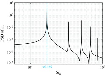


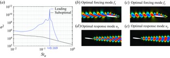


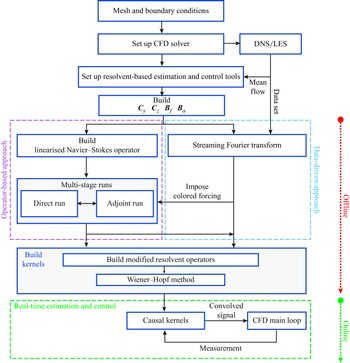
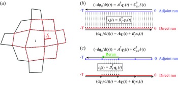


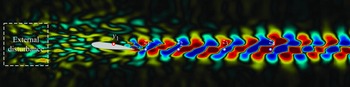
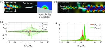


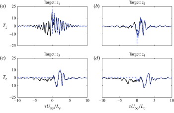


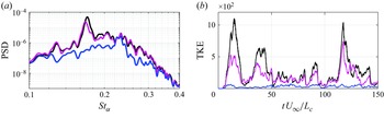


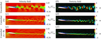


 Open access

