


1. Introduction
Arctic sea-ice extent has declined in all months over the modern satellite record (1979–present), particularly during late summer and early autumn (e.g., Nghiem and others, Reference Nghiem2007; Serreze and others, Reference Serreze, Holland and Stroeve2007; Emery and others, Reference Maslanik, Stroeve, Fowler and Emery2011; Screen and others, Reference Screen, Simmonds and Keay2011; Simmonds, Reference Simmonds2015; Kapsch and others Reference Kapsch, Graversen, Tjernström and Bintanja2016; Parkinson and DiGirolamo, Reference Parkinson and DiGirolamo2016; Kwok, Reference Kwok2018). Extent reductions from 2.7% (March) to 13% (September) per decade have been accompanied by reductions in ice thickness of up to 65% between 1975 and 2012 (Lindsay and Schweiger, Reference Lindsay and Schweiger2015; Fetterer and others, Reference Fetterer, Knowles, Meier, Savoie and Windnagel2017). The ice loss is making the Arctic Ocean more accessible to marine shipping, resource extraction, tourism and other activities (Meier and others, Reference Meier2014). Improved seasonal-scale forecasts of sea-ice conditions are increasingly needed to support such activities, but the 7–10 day limit of reasonably accurate weather prediction presents a formidable obstacle (Stroeve and others, Reference Stroeve, Hamilton, Bitz and Blanchard-Wrigglesworth2014; Serreze and others, Reference Serreze, Crawford, Stroeve, Barrett and Woodgate2016). Furthermore, as the ice thins, it weakens and becomes more susceptible to wind stress and other impacts of weather systems (Petty and others, Reference Petty, Hutchings, Richter-Menge and Tschudi2016; Serreze and Meier, Reference Serreze and Meier2019; Tschudi and others, Reference Tschudi, Meier and Stewart2019a), presenting further challenges to predictability.
How do cyclones affect the sea-ice cover? The effect varies seasonally, and can depend on the characteristics of a storm and the ice it passes over. Generally, thicker ice will be more resistant to both dynamic and thermodynamic effects, and so we expect smaller signals of concentration change in late winter, earlier in the time series, and in the area north of the Canadian Arctic Archipelago (where the thickest ice has historically been located). Some storms can bolster the ice, while others may weaken and diminish it (Morello, Reference Morello2013). Over the satellite record, there appears to be an increasing trend in cyclone strength, which has been associated with the reductions in September ice extent (Simmonds and Keay, Reference Simmonds and Keay2009), though generally seasons with fewer cyclones end with lower ice areas (Screen and others, Reference Screen, Simmonds and Keay2011). Other studies have shown a trend of increasing cyclone intensity due to a higher incidence of deep cyclones, particularly in winter, but a signal in summer is less distinct (Sepp and Jaagus, Reference Sepp and Jaagus2011; Akperov and others, Reference Akperov2019). Trends in frequency are unclear, and appear spatially variable (Zahn and others, Reference Zahn, Akperov, Rinke, Feser and Mokhov2018; Wickström and others, Reference Wickström, Jonassen, Vihma and Uotila2019).
A number of past studies have demonstrated that cyclonic surface winds can foster ice divergence (e.g., Thorndike and Colony, Reference Thorndike and Colony1982; Serreze and other, Reference Serreze, Barry and McLaren1989). Divergence in turn can promote greater melt by exposing low-albedo open water – increasing absorption of solar radiation in summer (Lei and others, Reference Lei, Gui, Heil, Hutchings and Ding2020) and increasing vulnerability of the ice to lateral melt in all seasons (Graham and others, Reference Graham2019b). Conversely, if sufficiently cold, divergence provides areas for new ice growth (Kriegsmann and Brümmer, Reference Kriegsmann and Brümmer2014). The strong winds associated with cyclone passage can also cause ridging and rafting, creating thicker ice more resistant to melting out in summer (Maslanik and others, Reference Maslanik2007).
These winds also augment mixing and foster heat transfer between the atmosphere, ice and ocean surfaces. An unusually strong cyclone passing over the central Arctic Ocean in August of 2012 (Simmonds and Rudeva, Reference Simmonds and Rudeva2012) appears to have reduced ice extent by mixing warm ocean waters upwards (Zhang and others, Reference Zhang, Lindsay, Schweiger and Steele2013). Exposure of the ocean surface by the ice divergence supplies moisture in addition to heat to the lower atmosphere, increasing cloud formation in autumn, contributing to a stronger downward longwave radiation flux (Kay and Gettelman, Reference Kay and Gettelman2009). Increased moisture loading and downward longwave radiation in the Arctic have been shown to be primary contributors to the reduced sea-ice cover and surface warming of the region (Luo and others, Reference Luo, Luo, Wu, Zhong and Simmonds2017; Lee and others, Reference Lee2017a, Reference Lee, Gong, Feldstein, Screen and Simmonds2017b). Local atmospheric moisture and heat content are further impacted due to wind-forced horizontal advection. This can lead to pronounced changes in air temperatures, either due to the movement of warmer air from the south, or colder air from the north. The intrusion of moisture from synoptic events has been a substantial factor in Arctic surface warming due to its impact on downward longwave radiation (Lee and others, Reference Lee, Gong, Feldstein, Screen and Simmonds2017b).
The increased cloud cover associated with storms affects the surface energy balance, with the overall cloud radiative effect leading to surface warming except in mid-summer (McCabe and others, Reference McCabe, Clark and Serreze2001; Dong and others, Reference Dong2010). In summer, the radiation balance depends on surface albedo, with cloudy skies resulting in greater energy input to high albedo surfaces (snow, ice) than sunny skies, but comparatively less to low albedo surfaces (leads, melt ponds) (Perovich, Reference Perovich2018).
Precipitation associated with cyclone passage over the Arctic Ocean can be in the form of snow or rain. Cyclones are the primary source of snow on sea ice in the Arctic (Webster and others, Reference Webster, Parker, Boisvert and Kwok2019), though the fraction of precipitation falling as rain is increasing and expected to dominate in the future (Screen and Simmonds, Reference Screen and Simmonds2012; Bintanja and Andry, Reference Bintanja and Andry2017). Rainfall decreases the surface albedo, resulting in greater energy absorption, while fresh snowfall increases surface albedo (Screen and others, Reference Screen, Simmonds and Keay2011) and slows melt in summer. Notably, snow reflects longer wavelengths less effectively than shorter wavelengths and so this albedo effect is seasonally dependent (Warren, Reference Warren1982). Additionally, fresh snow has a low thermal conductivity (Sturm and others, Reference Sturm, Perovich and Holmgren2002), so accumulation insulates the ice and inhibits the growth in winter (Ledley, Reference Ledley1991; Graham and others, Reference Graham2019b). However, high amounts of accumulation on the sea ice can also result in submersion of the sea ice surface and the formation of snow-ice (Webster and others, Reference Webster2018). These effects of snow accumulation are becoming more important as the ice thins. Winds also redistribute the snow, impacting the location and timing of melt pond formation in the spring (Webster and others, Reference Webster2018). Meanwhile, freshwater input to an exposed ocean surface in the form of either snow or rain will decrease salinity and foster ice growth if conditions are sufficiently cold.
In summary, the overall effect of cyclones on the sea-ice cover is complex. Recognizing this, we report here on a systematic analysis of the effects of cyclone passage on sea-ice concentration (SIC) spanning 40 years of data, for all seasons and over the entire Arctic Ocean. Rather than a single case study, looking at total sea-ice extent, or seasonal circulation patterns, we include all storms that have passed over any individual gridcell of ice in the Arctic Ocean to work toward a comprehensive understanding of the relationship between ice concentration and synoptic-scale cyclones. We also investigate how the sea ice's response may be changing as the Arctic system experiences profound warming. Our study makes use of SIC and motion vectors derived from satellite data, a record of cyclone locations and characteristics, along with air temperature and other variables estimated from an atmospheric reanalysis.
2. Data
2.1 Sea-ice concentration
We use SIC data from two passive microwave sources. As is convention, we consider gridcells with retrieved concentrations less than 15% to be ice-free in both datasets. The longer of the two datasets (available from 1979 to present) is the combined record from the Scanning Multichannel Microwave Radiometer (SMMR, 1979–1987, every other day), the Special Sensor Microwave Imager (SSMI, 1987–2007, daily) and the Special Sensor Microwave Imager/Sounder (SSMI/S, 2008–present, daily). SIC from these sources is derived from microwave brightness temperatures using the NASA Team algorithm and provided on the Equal-Area Scaleable Earth (EASE) Grid 2.0 (Brodzik and others, Reference Brodzik, Billingsley, Haran, Raup and Savoie2012) at 25 km spatial resolution by the National Snow and Ice Data Center (NSIDC) (Cavalieri and others, Reference Cavalieri, Parkinson, Gloersen and Zwally1996). This data product provides a nearly seamless timeseries of SIC, long enough to observe climatological relationships beyond inter-annual and decadal variability as well as to investigate trends (Comiso and Nishio, Reference Comiso and Nishio2008; Simmonds, Reference Simmonds2015).
A shorter but higher-resolution SIC dataset is available from the Advanced Microwave Scanning Radiometer 2 (AMSR-2) from July 2012 to present, at 10 km spatial resolution. It is derived using the NASA bootstrap algorithm (Comiso and Cho, Reference Comiso and Cho2013) and provided twice daily by the Japanese Aerospace eXploration Association (JAXA), once each from the ascending and descending passes of the satellite. We utilize the AMSR-2 data from the descending passes, as it is available at higher latitudes, and the orbit descends during local night (larger solar zenith angles over the Arctic Ocean in summer), mitigating the effects of surface melt that can contaminate ice concentration retrievals. Though this data product is too short to eliminate the effects of decadal variability, its higher spatial resolution allows us more insight along the coastlines and ice edge (Meier and others, Reference Meier, Fetterer, Stewart and Helfrich2015; Posey and others, Reference Posey2015; Pang and others, Reference Pang2018) and it is more likely to capture leads and polynyas (Beitsch and others, Reference Beitsch, Kaleschke and Kern2014; Nihashi and others, Reference Nihashi, Ohshima and Tamura2017).
Because the microwave signature of surface melt ponds is the same as ice-free water, errors of up to 30% in ice concentration are possible in summer (Comiso and Cho, Reference Comiso and Cho2013). Different stages of meltponding have differing impacts on the emissivity of the surface, and tie points needed for the concentration retrievals are difficult to establish in these conditions. Local atmospheric conditions also affect the satellite retrievals. Though the NASA Team and bootstrap algorithms include filters to account for some weather effects (Meier and others, Reference Meier, Fetterer, Stewart and Helfrich2015), water vapor, cloud liquid water content, and wind speeds can all bias the recorded brightness temperatures (Andersen and others, Reference Andersen, Tonboe, Kern and Schyberg2006). Errors tend to be largest at low ice concentrations.
2.2 Sea-ice motion
Use is made of the Polar Pathfinder Sea Ice Motion Vectors dataset (version 4). Velocity vectors are provided daily from 1979 onward by NSIDC at 25 km resolution (Tschudi and others, Reference Tschudi, Meier, Stewart, Fowler and Maslanik2019b). The data are provided on the EASE grid (Brodzik and Knowles, Reference Brodzik, Knowles and Goodchild2002), the predecessor to EASE 2.0 and offset by half a gridcell from the SIC information. Velocity values are provided in the u- and v-directions, relative to the gridcell boundaries. We use this dataset because it is primarily observation-based rather than model-based like other products (e.g., PIOMAS), though other evaluations may be beneficial in future work.
The vectors are developed using data from the International Arctic Buoy Program (IABP), winds from the NCEP/NCAR reanalysis, satellite passive microwave brightness temperatures (SMMR/SSMI/AMSR-E) and retrievals from the Advanced Very High Resolution Radiometer (AVHRR). To calculate ice motion from the satellite data, features in sequential brightness temperature fields are identified and tracked. The tracking is done by searching for the spatial offset that maximizes the cross-correlation over a set of pixels. The fields are least accurate in the summer, as with SIC, because surface melt and higher water content in the atmosphere affect the quality of the microwave retrievals (Emery and others, Reference Emery, Fowler and Maslanik1997). To mitigate summer melt contamination, tracking with AVHRR uses visible imagery in the summer, while infrared bands are used for the rest of the year. Supplementing the satellite sources, ice motion vectors are calculated from the NCEP/NCAR winds based on wind/ice drift relationships outlined by Thorndike and Colony (Reference Thorndike and Colony1982) – ice is assumed to move in the direction of the geostrophic wind, at 1% of its speed (Tschudi and others, Reference Tschudi, Meier and Stewart2019a). Finally, velocity fields from each data source are weighted depending on expected accuracy and blended together for the released product.
Apart from the issues of summer melt and weather effects, errors can be substantial in the marginal ice zone because the low-concentration ice tends to be dynamic with a high degree of deformation (Kwok and others, Reference Kwok, Schweiger, Rothrock, Pang and Kottmeier1998). In these areas, the features being tracked may change at shorter timescales than the temporal resolution of the satellite retrievals. Additionally, Kwok and others (Reference Kwok, Schweiger, Rothrock, Pang and Kottmeier1998) showed that motion fields based on winds and buoy motion overestimate actual ice velocities. Incorporation of data from individual buoys creates spurious circular features of higher velocity (Szanyi and others, Reference Szanyi, Lukovich, Barber and Haller2016), though version 4 of the data has improved on this issue. Aggregating the data over multiple days, as done here, helps to mitigate these problems.
2.3 Temperature, winds, precipitation and surface fluxes
Estimates of surface meteorology variables were obtained from the European Centre for Medium-Range Weather Forecasts (ECMWF) interim Re-Analysis (ERA-Interim). ERA-Interim output is available from 1979 to 2019, with six-hourly gridded values of three-dimensional atmospheric variables and three-hourly values for surface fluxes and other two-dimensional fields (Dee and others, Reference Dee2011). The data are available at 0.75° latitude $\times$ 0.75° longitude resolution and 27 pressure levels.
ERA-Interim has known biases in the Arctic, though in most cases performs similarly to or better than other reanalysis products. Positive surface temperature and humidity biases have been established by a number of studies (Lüpkes and others, Reference Lüpkes, Vihma, Jakobson, König-Langlo and Tetzlaff2010; Bromwich and others, Reference Bromwich, Wilson, Bai, Moore and Bauer2016; Graham and others, Reference Graham2019b). The warm bias is common across reanalyses, and ERA-Interim performs better than its successor, ERA-5, in spring and winter (Graham and others, Reference Graham2019b). The warm bias results in a positive bias in upward longwave radiation in spring and summer. There is also an upward bias in winter sensible and latent heats, as well as a positive downward shortwave flux in spring, and negative in summer. ERA-Interim also tends to slightly overestimate 10 m wind speeds in winter and summer, though underestimates them in spring. Notably, Jakobson and others (Reference Jakobson2012) found that ERA-Interim generally provides better representations of temperature, humidityand wind speed over the central Arctic Ocean compared to other reanalyses. Boisvert and others (Reference Boisvert2018) have shown that precipitation in ERA-Interim is realistic in magnitude and temporal distribution, though like other reanalysis products, it tends to include overly frequent trace (<1 mm) precipitation.
We analyze the fields of the 925 hPa air temperature, 10 m wind speed, precipitation (rain and snow), cloud cover, total column water and the radiative and turbulent fluxes at the surface. We chose the higher-level 925 hPa temperature because, during the summer melt season, it provides a better indication of the thermal state of the lower troposphere above sea ice than the 2 m temperature value, which tends to hover close to 0°C. Daily-averaged values are computed for all variables and bilinear interpolation is employed to regrid the values to both the 10 km (AMSR-2) and 25 km (combined record) passive microwave SIC grids.
2.4 Cyclone tracks and areas
We use output from the Crawford and Serreze (Reference Crawford and Serreze2016) advanced cyclone detection and tracking algorithm, an updated version of the Serreze (Reference Serreze1995) algorithm. It was applied to ERA-Interim sea level pressure (SLP) fields interpolated to the EASE 2.0 grid at 100 km resolution. This regridding must be completed because the unequal grid created by the convergence of longitudes in a latitude–longitude system biases cyclone frequency toward the pole. Mean SLP values in ERA-Interim have been found to successfully represent the observations in multiple studies (Lindsay and others, Reference Lindsay, Wensnahan, Schweiger and Zhang2014; Graham and others, Reference Graham2019a). Cyclone characteristics found by any particular study can be sensitive to the algorithm, reanalysis dataset and resolution (Pinto and others, Reference Pinto, Spangehl, Ulbrich and Speth2005; Raible and others, Reference Raible, Della-Marta, Schwierz, Wernli and Blender2008). However, those in ERA-Interim are in strong agreement with depictions from other reanalyses, particularly in the Northern Hemisphere (Hodges and others, Reference Hodges, Lee and Bengtsson2011; Screen and others, Reference Screen, Simmonds and Keay2011; Zahn and others, Reference Zahn, Akperov, Rinke, Feser and Mokhov2018). Overall, this algorithm detects fewer than average cyclones in the Northern Hemisphere as compared to 15 other algorithms using ERA-Interim as analyzed by Neu and others (Reference Neu2013), though it is well within the wide range found (Crawford and Serreze, Reference Crawford and Serreze2016). It is likely that this lower frequency is in part because the algorithm combines the tracks of multi-center cyclones into single systems. Additionally, algorithms that filter out areas of high topography (as Crawford and Serreze do) tend to identify fewer systems (Rudeva and others, Reference Rudeva, Gulev, Simmonds and Tilinina2014).
In the Arctic specifically, different tracking algorithms applied to ERA-Interim can diagnose minimum pressures of the same cyclone with differences up to 10 hPa; however, algorithms largely agree on positions of the cyclone centers (Simmonds and Rudeva, Reference Simmonds and Rudeva2014). In this study, we primarily focus on cyclone location, rather than intensities. Tracks are defined by the positions of SLP minima at 6 h time steps over the lifetime of each storm. Cyclone areas associated with each center are defined by the 100 × 100 km gridcells that lie within the outermost closed isobar in the SLP fields, and these areas are taken here as the areas in which the storms influence the conditions at the surface. We use nearest-neighbor regridding to transform the cyclone areas to the resolutions of our other datasets for use in investigating the SIC and atmospheric characteristics. Cyclones considered in this study are those that track into or across the central Arctic Ocean and its peripheral seas for at least two time steps.
3. Methods
3.1 Sea-ice concentration change
Our approach is to assess how SIC and surface meteorological conditions (e.g., energy fluxes, wind speed, precipitation) differ when a given area is influenced by a cyclone. We acknowledge that ocean conditions are also an important driver of changes to SIC, and that cyclones also impact ocean characteristics, but in this study, we focus on the atmospheric drivers of change. We look at the changes in SIC across the four seasons, defined as March-April-May (MAM), June-July-August (JJA), September-October-November (SON) and December-January-February (DJF). Spatial fields of sea-ice responses, as well as aggregated results, are examined for the seven regions defined in Figure 1.
Study area, showing boundaries of the Central Arctic Ocean and peripheral seas.

For a given cyclone, and for each 6 h time step that the cyclone exists, we identify the gridcells in the SIC and meteorology fields that are within the area of cyclone influence. As the cyclone location usually changes over the day, so does the area of influence of the cyclone and the gridcells in the SIC fields under that influence. There are four cyclone time steps per day (00.00, 06.00, 12.00 and 18.00 UTC). Hence, over the course of a given day, a SIC cell can either never be within cyclone influence, or be within an area of cyclone influence from one to all four of a day's time steps. For a gridcell to be counted as falling within cyclone influence for a given day, we required that it be under cyclone influence for at least two time steps in that day. This excludes gridcells with only fleeting cyclone influence. An example of 1 d of cyclone activity is shown in Figure 2 on the cyclone detection grid.
An example of 1 d of cyclone activity (6 November 2013). Shaded regions indicate areas within a cyclone's influence from 1 to 4 time steps in that day.

To investigate the SIC response to cyclone presence, we look at average concentration changes over a chosen period of 4 d. For each gridcell with cyclone influence for at least two time steps, we calculated the difference between SIC on that day and the SIC 4 d later. For example, if the SIC on the given day is 100% and 4 d later it is 80%, the 4 d total SIC change is -20%. The same difference can occur with a change from 50 to 30%. The units are in percentages, but represent areal changes in relation to an entire gridcell: 100 km2 for AMSR-2 and 625 km2 for the longer combined passive microwave record.
SIC can of course also change without any cyclone influence, in response to winds, ocean currents and the surface energy balance. There will also be day-to-day changes in SIC related to seasonal thermodynamic forcing – in summer, there will be a general tendency for SIC to decrease due to melt, while in autumn it will tend to increase because of ice formation. Thus, in most of the analyses that follow, we compare the values of cyclone-associated SIC change to the SIC changes when a given location is not within a region of cyclone influence.
The 4 d time scale of change was selected on the basis of a spectral analysis to find the time period between 1 and 7 d that SIC was most likely to change substantially in an individual gridcell, regardless of cyclone presence. This revealed the peaks at 3–4 d. We then calculated the difference in SIC change inside and outside of cyclone influence, finding the 4 d interval to provide a greater distinction between the two. Using an even number of days also enables the extension of our analysis back through the full satellite record, to utilize SMMR data (comprising the early part of the combined record) that are only available every second day. It must be noted that cyclones are likely to affect SIC on multiple time scales; for example, intense storms are likely to have a more rapid effect on the sea ice, while the effects of a slow-moving cyclone may tend to be more delayed. For the purposes of this study, we have chosen a single time scale, but this is a key issue that warrants further investigation.
Student's t-tests were used to assess the significance of differences in SIC within and outside of cyclone influence. This calculation is based on an effective sample size, accounting for lag-1 autocorrelation in the SIC changes. The effective sample size, or number of independent samples, (N*) in each of the time series was estimated with the following equation, from Wilks (Reference Wilks2011):

where N is the total number of data points in the time series, τ is the time lag (here 1 day) and γ(τ) is the autocorrelation at that lag. The autocorrelation was calculated with the following:

where σ is the standard deviation of the time series x(t), t 1 and t N are the starting and end points of the time series, respectively, and the prime denotes departures from the mean.
Values derived from AMSR-2 were also compared to those from SSMI/S for the overlapping period of data coverage (2012–2018) to assess the agreement. Use of the longer combined passive microwave record (1979–2018) enables an understanding of the inter-annual variability of sea-ice responses to cyclones and changes that may be occurring. We also calculate and examine the trends in these responses.
3.2 Sea-ice divergence
The procedures just described yield total SIC change within and outside of cyclone influence with no assumption of whether the SIC change is dynamic or thermodynamic in origin (or a combination of both). To try to separate these components, we use the sea-ice velocity vectors to estimate ice divergence rates. The SIC change remaining once the change due to divergence has been removed from the total SIC change is taken to be the thermodynamic component – ice melt or growth. Using ice velocity vectors in concert with the SIC data, divergence is estimated as follows:

where d is n days, du and dv are the changes in velocity in the x- and y-directions estimated by differencing the values of u and v across the boundaries of a gridcell, dx and dv are the horizontal distances between gridcells (here 50 km), and SICd−1 is the ice concentration from the previous day (because the ice motion vectors are determined by ice position in comparison to the previous day). A negative divergence value from this equation indicates more ice moving out of a particular gridcell than into it. A positive value indicates convergence, or more ice moving into a gridcell than out of it.
3.3 Caveats
As noted, SIC estimates in summer from passive microwave retrievals can be influenced by surface melt, which also affects the calculated 4 d SIC changes. Weather effects (i.e., water vapor, cloud liquid water, wind speed) can also influence the retrievals (Maslanik, Reference Maslanik1992; Emery and others, Reference Emery, Fowler and Maslanik1997; Andersen and others, Reference Andersen, Tonboe, Kern and Schyberg2006), particularly as cyclone winds advect water vapor into a region and promote cloud formation. The ice velocity vectors are prone to error in all seasons, particularly in summer and in the marginal ice zone. We are likely pushing the limits of the information that can be obtained regarding SIC change from these data. Errors in the ERA-Interim data are also likely, notably in the surface fluxes, which strongly depend on parameterizations. Additionally, the choice of looking at 4 d changes in SIC is a compromise. Over a 4 d period, other influences will be acting on the sea-ice cover; however, a time period of multiple days is necessary to evaluate relevant changes. Additionally, particularly strong or slow-moving storms may have an impact with a greater time delay, and consequences over differing time scales should be investigated in future efforts. All of these issues must be kept in mind when interpreting the results that follow.
4. Results and discussion
4.1 Cyclone frequency, meteorological conditions
The overall impact of cyclones on the sea-ice cover will vary, in part, due to spatial and seasonal variations in cyclone frequency. Figure 3 shows the average number of days of cyclone influence (days when a gridcell was under the influence of a cyclone for at least two time steps) across the Arctic Ocean by season, based on output from the detection and tracking algorithm over the period 1979–2018. The northern terminus of the North Atlantic storm track dominates cyclone influence on the Atlantic side of the Arctic, the exception being in summer when cyclone influence peaks over the central Arctic Ocean, largely reflecting the migration of cyclones into the area from northern Eurasia, as well as cyclogenesis over the Arctic Ocean itself (Serreze and Barrett, Reference Serreze and Barrett2008). These basic patterns of cyclone activity are well-known from previous studies (e.g., Serreze and others, Reference Serreze, Box, Barry and Walsh1993; Simmonds and others, Reference Simmonds, Burke and Keay2008; Tilinina and Gulev, Reference Tilinina, Gulev and Bromwich2014). Average days of cyclone influence per ~90 day season across our study region range from 5 to 40. This means that our data include least 200 days per gridcell of cyclone influence for each season over the combined satellite record, enabling robust statistical analyses.
Average number of days per season with at least two time steps of cyclone influence over the satellite record (1979–2018).

Surface conditions within individual cyclones and from storm to storm can vary substantially, but they are more similar to each other than to conditions outside of cyclone influence. Table 1 summarizes meteorological conditions aggregated for the entire Arctic Ocean over the 1979–2018 ERA-Interim record for days of cyclone influence and compared to days when there is no cyclone influence (cyclone influence minus no cyclone influence). All the difference values listed are statistically significant (p < 0.01). An immediately obvious potential effect of cyclones on SIC is that, except in autumn, lower tropospheric (925 hPa) temperatures during cyclone influence are about a degree lower compared to temperatures for no cyclone influence. In autumn, it is warmer during a cyclone though, on average, by less than a tenth of a degree. This may be due to warm air advection having a greater impact on the local temperature than in other seasons, and should be explored in future study.
Differences between average meteorological conditions when there is a cyclone and when there is not (bold). All differences are statistically significant (p < 0.01). Average in-cyclone conditions are given in parentheses. Fluxes are positive downward.

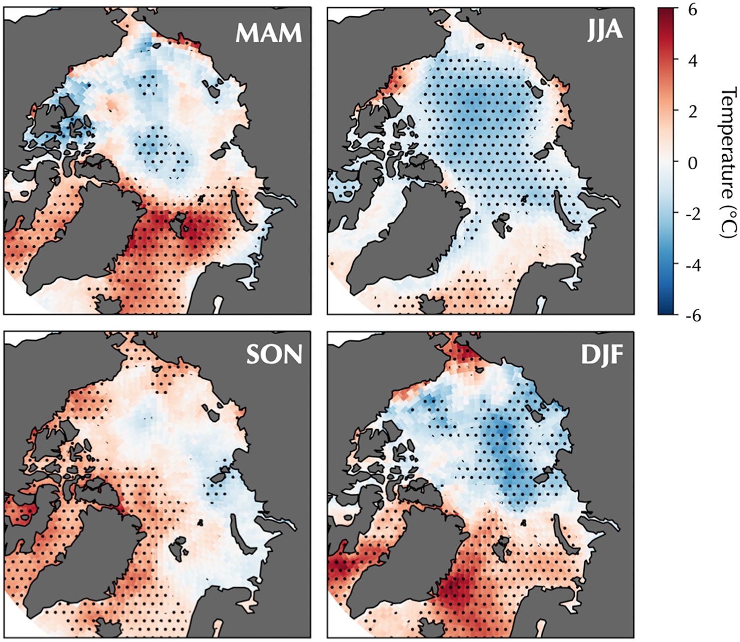
The spatial pattern of these conditions is further illuminating – the summaries of Table 1 mask interesting variation across the region (Fig. 4). In all seasons, the periphery of the Arctic Ocean has a tendency to be warmer than average under cyclone influence, while the central Arctic is likely to be cooler. Except for in autumn, cooler conditions under cyclone influence away from the Atlantic side of the Arctic Ocean contrast with warmer conditions over the Atlantic side of the Arctic Ocean (which is largely ice-free year round, apart from Baffin Bay and the northern Barents Sea). The Atlantic signal points to the influence of warm air advection by cyclones entering the Arctic Ocean along the northern terminus of the North Atlantic storm track. By contrast, it is known that mature cyclones over the central Arctic away from the Atlantic sector tend to be cold-cored (e.g., Serreze and Barry, Reference Serreze and Barry1988; Tanaka and others, Reference Tanaka, Yamagami and Takahashi2012; Rinke and others, Reference Rinke2017). The effect of these cold-cored cyclones is most apparent in summer, in considerable part because of the high frequency of cyclone activity over the central Arctic Ocean in this season (Fig. 3).
Average temperature difference at 925 hPa under cyclone influence compared to no cyclone influence (2012–2018). Stippling indicates differences that are statistically significant (p < 0.05).
Turning back to Table 1, we see that according to ERA-Interim, cloud cover associated with cyclone influence is on average 2–10% greater than non-cyclone conditions, though overall our study area is very cloudy, as expected. Notably, though the differences in total cloud cover are 10% or less, the differences in medium-level (defined as 0.8 SLP to 0.45 SLP) cloud cover fall between 22 and 29% throughout the seasons. Differences in high- and low-level clouds (not shown) are less pronounced, at 8% or less. From this, we conclude that not only is there greater cloud fraction during cyclones, but the cloud layer is thicker and therefore able to scatter and reflect greater amounts of radiation – decreasing shortwave but increasing longwave radiation reaching the surface. The increased cloudiness also accounts, in part, for the increased total column water in autumn, winter and spring. While the absolute amount of column water in the summer is greatest, it is actually slightly below non-cyclone conditions, by 0.4 kg m−2. This may be related to the smaller increase in downward longwave radiation associated with cyclone presence in summer.
Clouds reduce the amount of spring and summer solar radiation reaching the surface by 30–40 W m−2 (Table 1). In autumn and winter, there is no appreciable solar flux, but ERA-Interim captures the expected corresponding increase in the longwave radiation flux to the surface. The increase in the longwave flux acts to make the net radiation (all wave) budget at the surface less negative in autumn and winter (when the shortwave radiation is essentially absent). The reduction in the shortwave flux exceeds the increase in the longwave flux in spring and summer – though the amount of energy absorbed will depend on the surface albedo (Perovich, Reference Perovich2018). The decreased shortwave flux contributes to the lower 925 hPa temperatures over the Arctic Ocean in summers during cyclone influence, and perhaps also in spring (Fig. 4). The overall cooling effect of clouds in summer is well established (e.g., Wang and others, Reference Wang, Key, Wang and Key2005; Dong and others, Reference Dong2010). In spring, cloud cover is generally expected to have a warming effect at the surface, though our data show the reduction in shortwave energy by storm clouds outweighing the increase in longwave energy to the surface. It may be that ERA-Interim does not fully capture cloud radiative effects; this merits further study. The cloud effect likely also plays into the generally small temperature differences between cyclone and non-cyclone conditions over the ice-covered Arctic Ocean during autumn.
Cyclones are of course also associated with precipitation. For all seasons, snowfall and rainfall are greater when cyclones are present (Table 1). Precipitation, as represented in ERA-Interim, is primarily snow in spring, autumn and winter. While precipitation falls primarily as rain in summer, snowfall is still common in this season, especially in the higher latitudes of the Arctic Ocean, where it increases the albedo, again consistent with the cooler summer conditions under cyclone influence. In warm months, this increased albedo will slow surface melt. Snow that falls onto the sea ice also creates a layer of insulation, resulting in slower ice growth in cold months. However, if enough snow falls to cause submersion of the ice surface, the snow will be flooded and result in snow-ice, creating thicker floes. If the precipitation falls on exposed ocean, it will decrease the local salinity, promoting sea-ice formation (assuming low enough temperatures). When falling as rain on the sea ice, precipitation will result in a decrease in albedo of the surface. In this case, it can accelerate melt.
In spring, summer and autumn, wind speeds are about 1 m s−1 higher during cyclone influence, with a smaller difference in winter (0.76 m s−1) (Table 1). Aside from resulting in more ice motion, this should also foster larger turbulent heat exchanges. For spring, autumn and winter, the surface sensible heat flux is indeed more strongly upward under cyclone influence (~2 W m−2), cooling the surface, but the difference is most pronounced in winter (~9 W m−2). This is also when air temperatures are lowest, meaning that any leads in the ice cover will create large temperature gradients at the surface. The sensible heat flux associated with cyclone presence is slightly more positive (downward) in summer when the surface is melting, so this is not a mechanism contributing to the greater ice concentrations. The winter latent heat flux is more strongly upward (negative, removing energy from the surface and putting water vapor into the atmosphere) under cyclone influence – by 5 W m−2. Latent heat fluxes are also more negative in spring and autumn under cyclone influence, but not in summer. It is important to note that the turbulent fluxes depicted by ERA-Interim represent regional averages and will not capture the much-larger localized fluxes strongly cooling the surface over open water areas that may lead to rapid ice growth. As has long been known (e.g., Maykut, Reference Maykut1978), cold-season turbulent fluxes over open water or thin ice can be 1–2 orders of magnitude greater than over adjacent thicker ice. We will return to this issue later.
4.2 Total sea-ice concentration changes
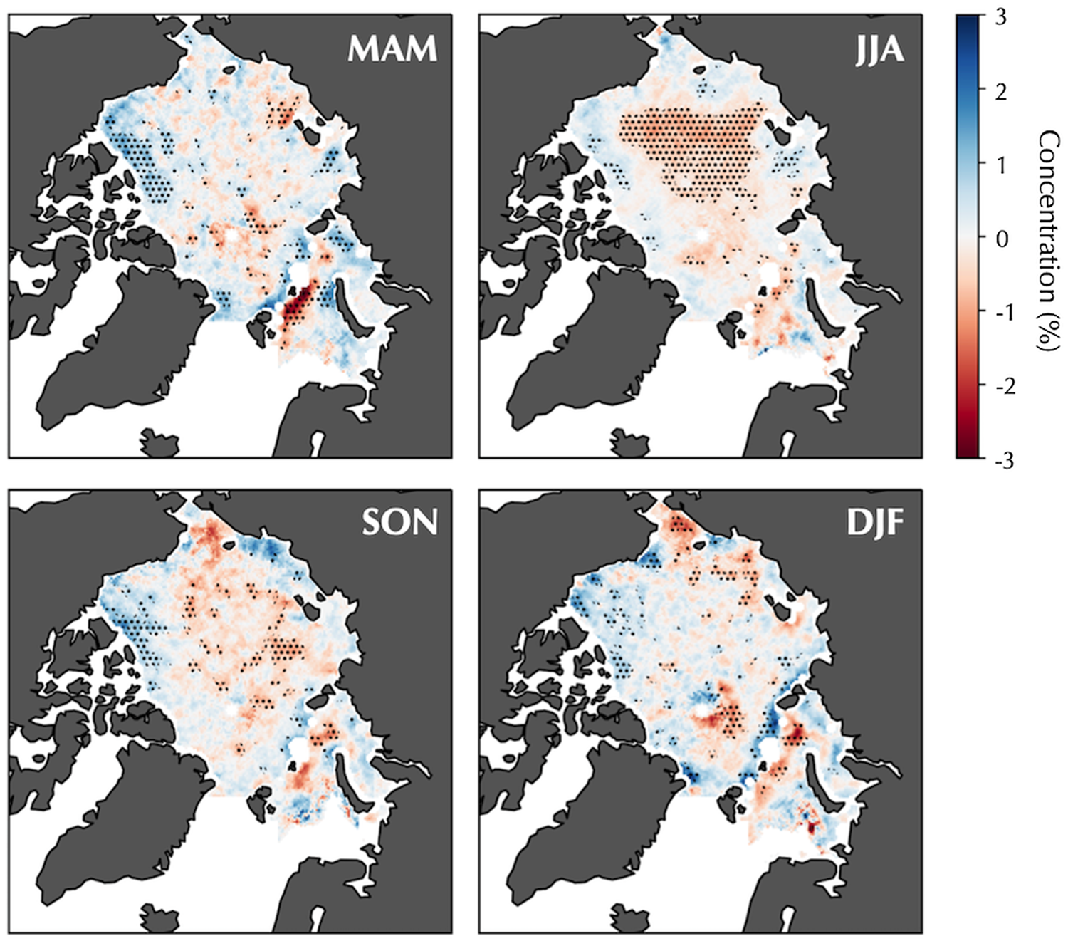
Averaged over the combined (1979–2018) passive microwave record, gridcells tend to have either approximately the same or a higher SIC 4 d after cyclone influence than in the absence of cyclone influence (Fig. 5). The largest areas of statistically significant positive differences are in summer and autumn, but are in different regions. There are fewer regions of statistically significant SIC change in winter and spring associated with cyclones. This may be, in part, due to the overall greater ice concentration in these seasons; areas with 100% ice cover, or nearly 100%, will be more resistant to change.
Average differences between 4 d SIC change with and without cyclone influence. Blue shows greater SIC associated with cyclone passage, either due to greater increase or lesser decrease in SIC. Stippling indicates differences that are statistically significant (p < 0.05).

In summer, all of the peripheral seas except the Barents have statistically higher SIC 4 d after cyclone influence compared to no cyclone influence. In the Barents Sea, there are some large negative differences near the ice margin. In autumn, the Chukchi and East Siberian Seas show no robust signal, but there are significant signals of higher SIC across much of the central Arctic Ocean, north of the Canadian Arctic Archipelago and in the Kara and Laptev Seas. In all seasons but summer, the largest positive differences are in the Barents Sea, perhaps in part due to the high frequency of cyclone influence there (Fig. 3); however, the limited amount of sea ice in the region, even in winter, also means that there are fewer data points to establish confidence in these values.
A regional breakdown of SIC change follows in Figure 6. While the maps in Figure 5 show the average differences in SIC within and outside of cyclone influence, here we break down the results separately – into SIC changes within cyclone influence, SIC changes outside of cyclone influence and SIC changes based on all observations. We include the averages from the full time series, as well as from the period 2012–2018 from the AMSR-2 record and the overlapping part of the combined passive microwave record, which for 2012–2018 is based on SSMI/S.
Four-day SIC change (%) by region and season, comparing gridcells within cyclone influence (orange), outside of cyclone influence (blue) and the average of all observations (gray). Bars show values derived from SMMR/SSMI for the full time series (1979–2018). Values from AMSR-2 are marked by crosses, and values from SSMI for the same time period as AMSR-2 (2012–2018) are marked by diamonds.

An interesting picture emerges. In summer, for all conditions, 4 d SIC changes are negative in all regions except cyclone gridcells in the Beaufort Sea and Central Arctic Ocean, which hover near zero change. Generally, changes within cyclone influence are less negative than those outside of cyclone influence. We also see that the climatology of SIC change (the gray bars) is very similar to the non-cyclone values. This is expected, as the Arctic is typically under non-cyclone conditions. The changes in SIC are relatively small over the central Arctic Ocean and more pronounced in the marginal seas. The situation is reversed in autumn – whether or not there is cyclone influence, the 4 d SIC change is positive, again much larger in the marginal seas than over the central Arctic Ocean, but the increase in SIC is greater when there is cyclone influence than when there is no cyclone influence. We also see that, overall, the values derived from the later time period tend to show greater absolute changes than the full time series. This relationship is discussed later in our ‘Trends’ section. With some exceptions (discussed shortly), the two datasets (AMSR-2 and SSMI/S) are in general agreement with respect to these SIC changes. Consistent with Figure 5, the values of SIC change in winter and spring are generally much smaller.
In essence, it is the smaller magnitudes of the negative SIC change during cyclone conditions compared to outside cyclone influence in summer (a negative minus a larger negative) and the larger increase in SIC inside compared to outside cyclone influence in autumn (a positive minus a smaller positive) that result in the positive differences in SIC change shown in Figure 5 for these seasons. The smaller differences in SIC with and without cyclone influence for winter and spring, and their correspondence with the results in Figure 5, can be similarly explained.
These results indicate that: (a) in summer, while SIC is generally decreasing (more strongly over the marginal seas than over the central Arctic Ocean), the overall effect of cyclones is to slow the rate of decline in ice concentration, i.e., to work against the seasonal cycle; (b) in autumn, while SIC is generally increasing (again more strongly over the marginal seas than over the central Arctic Ocean), the overall effect of cyclones is to augment the rate of increase in concentration, i.e., to work in the same direction as the seasonal cycle. Although the impact in spring is the same as in summer, and the impact in winter follows that for autumn, the SIC differences are neither as large nor as geographically extensive in these two seasons. As mentioned previously, this is likely because areas with close to 100% ice cover are more resistant to changes than those with lower concentrations.
The results so far further suggest that any cyclone-induced SIC decrease due to divergence is outweighed by thermodynamic influences that work in the opposite direction (weaker melt in summer, stronger ice growth in autumn). Notably, from Figure 4, away from the largely ice-free Atlantic sector, summer conditions within cyclone influence are cooler than outside of cyclone influence. Additionally, as indicated in Table 1, the largest impact of cyclone presence on the surface energy balance in summer is to decrease the downward shortwave radiation, and this will also result in slower or interrupted melt. However, this explanation does not work for autumn, when air temperatures within and outside of cyclone influence are not much different, and there is more longwave radiation to the surface (Table 1) outweighing the decrease in downward shortwave and turbulent fluxes. Snowfall onto the ice will increase the albedo and may prevent some of this energy from being absorbed – though rainfall will have the opposite effect. It may be that the consequences of cyclone-induced divergence are more important, or that stronger turbulent heat exchanges (which are not well captured by the ERA-Interim) over any leads formed will quickly freeze over. Additionally, greater amounts of both liquid and solid precipitation under cyclone influence will freshen the ocean surface, and may be promoting ice growth. Conversely, it may be that our results are influenced by weather effects on the passive microwave retrievals associated with the passage of cyclones.
As noted, there is basic agreement between the SIC changes depicted in AMSR-2 and SSMI/S, a clear exception being in the Barents Sea (Fig. 6). AMSR-2 and SSMI/S are least likely to agree when either the region or the season dictates minimal sea-ice presence. The best agreement occurs with values averaged over the entire region and for the central Arctic Ocean sector. The Beaufort Sea is also fairly well matched, aside from autumn, when the concentration change observed in SSMI/S is of lower magnitude than observed in AMSR-2. The inability of SSMI/S (with its coarser resolution) to resolve conditions as close to the coastline as AMSR-2 may partly account for the differences; for example, most of the SIC increase in the Beaufort associated with cyclones is near the shore (Fig. 5). Additionally, the satellites that carry the instruments are on different orbits, and therefore will not capture exactly the same sea-ice conditions.
Histograms of SIC change in marginal seas for summer and autumn (the two seasons with the strongest SIC change signals), based on the higher resolution AMSR-2 product, offer some additional insights (Fig. 7). While most 4 d SIC changes stay within ±15%, here we show that there can be much larger changes within and outside of cyclone influence. Some changes reach 100%, i.e., gridcells were fully ice-covered and then became ice-free, or vice versa. Gridcells under cyclone influence are more likely to have a positive SIC change and are less likely to have negative SIC change than those outside of cyclone influence. Notably, not all SIC changes in a particular season have the same sign – positive and negative concentration changes both occur in summer and autumn. As these are total SIC changes, the values are a combination of thermodynamic and dynamic changes, so either motion or formation/melt (or both) are inducing these values. Particularly in these seasons where there is a larger marginal ice zone, with lower overall ice concentrations, motion of the ice occurs more freely. Additionally, more exposed ocean surface allows for new ice growth, but also increased lateral melt. In summer, greater melt is expected, and in autumn, more ice formation is expected. This is reflected in our results – negative SIC changes are overall more likely in summer, and positive SIC changes are more likely in autumn, independent of cyclone influence. A notable exception to the SIC change relationship inside and outside of cyclone influence is the Barents Sea in summer: gridcells changing from fully ice-covered to fully open ocean are more likely to occur when there is cyclone influence than when there is no cyclone influence. This is in contrast to the other Arctic seas, where gridcells completely opening up is more likely to occur without cyclone influence. It is possible that this is in part due to the greater amounts of open water, increasing ice mobility due to decreased internal stresses. Additionally, the Barents Sea is particularly susceptible to cyclones coming up the North Atlantic storm track from the south, bringing heat to the region.
Frequency of gridcells from AMSR-2 with 4 d SIC change greater than 15% in the Barents, Kara and East Siberian Seas during summer and autumn (2012–2018). Comparisons between cyclone-influenced gridcells (orange), non-cyclone influenced gridcells (blue) and all observations (gray) are shown.

4.3 Dynamic vs. thermodynamic changes
Rates of estimated SIC change linked to sea-ice divergence, whether within or outside of cyclone influence, vary greatly by region and season (Fig. 8). Estimated rates can strongly depend on which SIC dataset is used in the calculation, but for most regions and seasons, computations using the two passive microwave sources yield SIC changes of the same sign. The variability due simply to differing data sources is important to note, as it is indicative of the uncertainty in these calculations, how the values may be changing over time, as well as the effect of resolution in capturing ice motion – especially considering the large spatial variation we observe (discussed later). For the most part, the best agreement occurs when averaged over the full study area, reducing the noise.
Four-day SIC change (%) due to ice divergence for all seasons and regions, comparing gridcells within cyclone influence (orange), outside of cyclone influence (blue) and the average of all observations (gray). Bars show values derived from SMMR/SSMI for the full time series (1979–2018). Values from AMSR-2 are marked by the crosses, and values from SSMI for the same time period as AMSR-2 (2012–2018) are marked by the diamonds. The apparently missing marker from SSMI/S for the Chukchi Sea cyclone value in autumn is due to its extreme value of almost −4%.

Overall, divergence (resulting in negative SIC change) is more likely than convergence. The variations evident in different datasets are important to recognize as there is a substantial amount of uncertainty in the amount of ice motion. The best agreement occurs over the full region and in seasons/regions where the values are small. In regions such as the Chukchi and Laptev Seas, we observe greater rates of divergence in the more recent time period than over the full satellite record. While average total SIC changes over individual regions can reach 10% over 4 d, average divergence-induced SIC changes (whether within or outside of cyclone influence) stay below 2%. The most substantial divergence-induced SIC changes are found to be in the Chukchi Sea in summer (negative), autumn (negative) and winter (positive) and in the Laptev Sea and Kara Seas in spring, autumn and winter (all negative).
The spatial patterns of the differences (within cyclone influence minus outside of cyclone influence) in divergence-induced SIC change based on the combined (1979–2018) passive microwave record follow in Figure 9. There is a mix of positive and negative differences. This is expected, as any ice that moves out of one gridcell must move into another. If a cyclone is expected to induce divergence of ice, it must also induce convergence elsewhere. Because of this, as well as the limitations of the ice motion dataset, fields of divergence values are noisy. This variability shows us that there is not a clear and consistent pattern of cyclonic winds resulting in ice divergence, despite established expectations. There is a coherent region over the central Arctic Ocean of negative SIC change differences in summer, however. This is also present in autumn, but less well expressed. Notably, there is also a broadly consistent pattern of positive SIC differences along the shores of the Canadian Arctic Archipelago during cyclone influence in all seasons, though it is best exhibited in spring and autumn.
Average differences between 4 d motion-induced SIC change with and without cyclone influence (1979–2018). Blue shows greater SIC associated with cyclone passage, either due to greater increase or lesser decrease. Stippling indicates differences are statistically significant (p < 0.05).
To reiterate, during summer, the total reductions in SIC within cyclone influence tend to be smaller than the reductions in SIC outside of cyclone influence (Fig. 6). Lower tropospheric conditions during summer are cooler during periods of cyclone influence as compared to no cyclone influence (Fig. 4). It is evident from Figure 8 that the effect of lower temperatures on reducing melt will, depending on the region, either work in the same direction as the (smaller) divergence-induced SIC changes or work against them, but still dominate. For autumn, the increases in SIC within cyclone influence tend to be larger than the increases in SIC outside of cyclone influence (Fig. 6). However, there is no coherent cold signal associated with cyclones; over some areas of the ice cover, conditions are actually warmer during cyclone influence (Fig. 4).
Why, then, is there a more positive SIC change in autumn during cyclone influence as opposed to no cyclone influence, especially since (according to ERA-Interim, see Table 1) the downward longwave flux to the surface is also greater during cyclone influence? One possibility is that it is sufficiently cold in autumn (on average −11°C in cyclones, Table 1) so that leads freeze over quickly in response to larger turbulent fluxes (linked to higher wind speeds) accompanying cyclones. Cyclone-associated precipitation acting to freshen the surface in leads would also facilitate ice growth. Snowfall onto sea ice insulates it and slows growth, but it increases the albedo, resulting in less energy absorption. The balance between these effects will largely depend on the thickness of the ice, and will vary substantially over small spatial scales. Such local effects cannot be expected to be captured by the resolution of ERA-Interim. However, another possibility is that the observed differences in SIC change within and outside of cyclone influence are, at least in part, influenced by weather effects on the passive microwave retrievals.
4.4 Trends
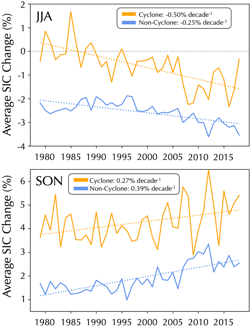
The statistics of SIC change are not stationary; Figure 10 shows how the 4 d SIC changes vary by year inside and outside of cyclone influence and their temporal trends over the full satellite record in summer and autumn. We expect that these trends can primarily be attributed to a combination of generally warmer conditions and a thinner ice pack. Looking first at summer, for every year, the average SIC change is more negative outside of cyclone influence than within cyclone influence. While the SIC changes both within and outside of cyclone influence vary from year to year, over time the SIC changes are becoming more negative. Furthermore, the trend toward more negative SIC change within cyclone influence (−0.50% per decade) is stronger than the trend for SIC change outside of cyclone influence (−0.25% per decade). Both of these trends are statistically significant, as is the difference between them (p < 0.01). The −0.50% per decade trend translates to 3.1 km2 more SIC decrease per 625 km2 gridcell than 10 years prior, while −0.25% per decade trend translates to 1.6 km2 more SIC decrease per gridcell than 10 years prior. By contrast, in autumn, there is a positive trend in the 4 d SIC change of 0.39% per decade outside of cyclone influence, compared to 0.27% per decade within cyclone influence. Both trends are significantly different from zero (p < 0.05), though the difference between the two is not statistically significant. If these summer and autumn trends continue, then the 4 d SIC changes associated with cyclone influence will become increasingly similar to those that occur outside of cyclone influence. Effectively, these trends imply that the influence of cyclones on ice concentration is becoming less important with time.
Average annual summer and autumn SIC change (%) for the entire Arctic Ocean domain within and outside of cyclone influence (solid lines) and linear trends (dotted lines).
Regional trends over the period 1979–2018 in the 4 d SIC change within and outside of cyclone influence are summarized in Table 2 for each season. The trends in each region typically follow those aggregated for the entire study area (Fig. 10), but there are exceptions. In summer, there are negative trends in total SIC change in most regions, i.e., 4 d SIC changes both within and outside of cyclone influence are becoming more negative. This likely is due to greater rates of summer melt as the region warms and the ice thins. The summer trend is weakest over the central Arctic Ocean, and there is essentially no summer trend in the Barents Sea for the within-cyclone case. There are also negative trends in spring SIC change without cyclone influence – SIC is decreasing at greater amounts than it used to, but there are no statistically significant trends in the SIC change associated with cyclones.
Trends (% decade−1) in seasonal average SIC change during conditions of cyclone influence and during conditions of no cyclone influence. Underlined trend pairs are statistically distinct from each other at p < 0.05. Bold values indicate trends statistically distinct from zero at p < 0.05, italics indicate p < 0.01.

For autumn and winter, all significant trends in 4 d SIC change are positive, apart from the Barents Sea sector in autumn. Stated plainly, SIC is increasing faster in cold months than it did in the past. This is consistent with the increasingly extensive areas of open water at summer's end able to freeze over. For example, there has been an increase of 1.49% in SIC change per decade in the Beaufort Sea, translating to over 9 km2 more ice growth over 4 d today than 10 years ago per 625 km2 gridcell. The autumn trends in SIC change associated with cyclones are larger than those without cyclone influence; however, the differences between cyclone-influenced SIC change trends and those outside of cyclone influence do not reach statistical significance, aside from the Barents Sea. The difference in Barents Sea trends is in the opposite direction, indicating that SIC is increasing slower than in the past in this region.
We also calculated trends in the SIC change associated with divergence, but few are statistically significant. The largest computed trend is for winter in the Laptev Sea (−0.4% per decade with cyclone influence), but it is statistically indistinguishable from the trend occurring without cyclone influence. Essentially, winter SIC decrease due to divergence is occurring at greater rates in the Laptev than in the past, but cannot be related to cyclone activity.
5. Summary and conclusions
Our results argue that the overall influence of cyclones is to work against the climatological decrease in SIC during summer, and augment the climatological increase in SIC during autumn, with generally smaller influences in winter and spring. Over most of the region, particularly in the marginal ice zone, there is statistically (p < 0.05) greater SIC after cyclone influence than there would be otherwise. Separating the thermodynamic and dynamic drivers of the SIC change associated with cyclone passage is challenging; the divergence calculations are noisy, perhaps pushing past the accuracy limits of the ice velocity fields. Further work incorporating other sources of ice motion information may offer greater insight to our mixed findings on cyclones as a mechanism for ice divergence. Overall, our results show that thermodynamic effects are the primary driver of SIC change related to cyclone passage. In summer, the cooler conditions associated with cyclone influence, in conjunction with generally small divergence-induced SIC changes, argue for a dominant effect of reduced melt. The situation in autumn is less clear. Divergence-induced SIC change and rapid ice formation in leads may be important. However, surface melt effects in summer, and weather effects in both summer and autumn, which can contaminate the passive microwave SIC retrievals, are cause for concern. One potential path forward to addressing these issues is to use synthetic aperture radar (SAR) data to assess SIC changes inside of cyclone influences. Analysis of turbulent flux and other data collected during the MOSAiC expedition over the central Arctic Ocean may also prove useful (https://www.mosaic-expedition.org/). These data and further study of the reanalysis information may lead to improved understanding of the mechanisms for the observed concentration changes related to cyclone passage, beyond the correlative relationships we have shown here. With this additional work, the varying time scales of cyclone effects on sea ice may be further illuminated, particularly as the ice pack continues its decline.
Based on the results we have presented, cyclones could be considered a mechanism promoting and preserving ice extent in the Arctic. This is in contrast to some recent studies (e.g., Zhang and others, Reference Zhang, Lindsay, Schweiger and Steele2013; Graham and others, Reference Graham2019b) that have shown cyclones as a mechanism for sea-ice loss. However, the relationship that we have reported on here is not static. We find statistically significant trends in the total 4 d SIC change during summer (negative) and autumn (positive) associated both with cyclone and non-cyclone influenced gridcells. Larger trends were found with the cyclone cases. If these summer and autumn trends continue, and acknowledging the caveats just mentioned, then the 4 d SIC changes associated with cyclone influence will become increasingly similar to those that occur without cyclone influence. This implies that as the sea-ice cover continues to thin and retreat, the influences of cyclones on SIC helping to preserve it are declining. Indeed, it may be that cyclones are instead becoming more likely to cause decreased concentration, resulting in the trends we find in overall SIC changes.
Acknowledgments
This study was supported by NSF grants PLR 1603914 and OPP 1748953. We thank the anonymous reviewers and editor for their helpful comments and suggestions.


 Open access