


1. Introduction
The small scales in homogenous isotropic turbulence are typically quantified by means of the dissipation rate,  $\varepsilon = 2\nu {S_{ij}}{S_{ij}}$, and the enstrophy, $\varOmega = {\boldsymbol{\omega }^2}$, which characterize the local energy loss and rotation rate, respectively. Here, Sij is the strain rate tensor, ω is the vorticity vector and ν is the kinematic viscosity. As a matter of convenience, ε will simply be referred to as dissipation throughout the paper. It is well known that the instantaneous dissipation and enstrophy structures are different with distinct physical implications (e.g. Chacin & Cantwell Reference Chacin and Cantwell2000; Moisy & Jiménez Reference Moisy and Jiménez2004; Ganapathisubramani, Lakshminarasimhan & Clemens Reference Ganapathisubramani, Lakshminarasimhan and Clemens2008; Elsinga et al. Reference Elsinga, Ishihara, Goudar, da Silva and Hunt2017, and figure 1). The instantaneous small-scale structure of intense enstrophy is typically tube-like and linked to strong lateral accelerations which repel heavy particles and attract light particles or bubbles (Mathai, Lohse & Sun Reference Mathai, Lohse and Sun2020), while intense dissipation, or strain, has a sheet-like structure and is associated with particle clustering (Squires & Eaton Reference Squires and Eaton1991), droplet/particle collisions (Perrin & Jonker Reference Perrin and Jonker2016), droplet deformation and breakup (Vela-Martín & Avila Reference Vela-Martín and Avila2021) and the production of intense scalar gradients (Elsinga & da Silva Reference Elsinga and Da Silva2019). However, these different small-scale enstrophy and dissipation structures tend to cluster within the same large-scale shear layers (e.g. Ishihara, Kaneda & Hunt Reference Ishihara, Kaneda and Hunt2013; Elsinga et al. Reference Elsinga, Ishihara, Goudar, da Silva and Hunt2017 and figure 1).
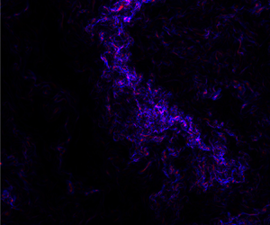
Intense enstrophy (red) and intense dissipation (blue) are associated with different small-scale structures, which tend to cluster within the same large-scale layer structure. The plot shows a 0.73L × 0.60L plane from the DNS data of homogenous isotropic turbulence at Reλ = 1131 by Ishihara et al. (Reference Ishihara, Kaneda, Yokokawa, Itakura and Uno2007). The colour scales range from zero to 20 % of the maximum of each quantity within the plane.

A statistical description of the enstrophy and dissipation intensities is provided by their moments and maxima, whose Reynolds number dependencies are an outstanding issue. The issue is of considerable practical interest, since much of our understanding of the aforementioned physical processes relies on data obtained at relatively low Reynolds numbers, while industrial and environmental applications are typically at much higher Reynolds numbers.
Results from direct numerical simulations (DNSs) have shown that enstrophy is more intermittent than dissipation resulting in a wider probability density function (PDF) (Kerr Reference Kerr1985; Chen, Sreenivasan & Nelkin Reference Chen, Sreenivasan and Nelkin1997; Donzis, Yeung & Sreenivasan Reference Donzis, Yeung and Sreenivasan2008; Yeung, Donzis & Sreenivasan Reference Yeung, Donzis and Sreenivasan2012), which is probably related to the fact that enstrophy is tube-like and dissipation is sheet-like. Furthermore, the second-order moments of the dissipation,  $\langle {\varepsilon ^2}\rangle $, and enstrophy, $\langle {\varOmega ^2}\rangle $, scale differently at low Reynolds numbers (Reλ < 83, Kerr Reference Kerr1985). Here, $\langle \cdots \rangle $ indicates averaging and Reλ is the Reynolds number based on the Taylor scale. Specifically, the Reynolds number scaling exponent for $\langle {\varOmega ^2}\rangle $ is larger than for $\langle {\varepsilon ^2}\rangle $. However, in the limit of infinite Reynolds number, dissipation and enstrophy are expected to scale the same based on certain theoretical considerations, which involve the finiteness of the pressure fluctuations (Nelkin Reference Nelkin1999) or the structures inducing enstrophy and dissipation being localized (He et al. Reference He, Chen, Kraichnan, Zhang and Zhou1998). In that case, the ratio of the nth-order moments, ${\nu ^n}\langle {\varOmega ^n}\rangle /\langle {\varepsilon ^n}\rangle $, remains finite and approaches a constant at infinite Reynolds number. At relatively high Reynolds numbers, i.e. 140 < Reλ < 1000, the ratio of the second-order moments of enstrophy and dissipation normalized by their respective means is still not exactly constant, but may be seen to slowly approach a value close to 2 (Ishihara et al. Reference Ishihara, Kaneda, Yokokawa, Itakura and Uno2007; Yeung et al. Reference Yeung, Donzis and Sreenivasan2012). This suggests that the PDF widths remain different even if dissipation and enstrophy eventually scale the same. The ratios of higher order moments have not been conclusively shown to approach to a constant. Furthermore, recent results up to Reλ = 1300 have suggested that enstrophy and dissipation may scale together when averaged over inertial range scales, but not when considering small scales (Yeung & Ravikumar Reference Yeung and Ravikumar2020). If the theory is correct, then the Reynolds number scaling exponent needs to depend on Reλ, at least for one of these quantities, to match the scaling differences observed at finite Reλ with the scaling similarity at infinite Reλ. Indeed, the present observations support this conjecture (§ 3).
Some further evidence for a developing scaling exponent comes from the flatness factor of the longitudinal velocity gradient. In homogeneous isotropic turbulence, the second-order dissipation moment is proportional to the flatness factor of the longitudinal velocity derivative, i.e.  $\langle {(\partial u/\partial x)^4}\rangle /{\langle {(\partial u/\partial x)^2}\rangle ^2} = {\textstyle{{15} \over 7}}\langle {\varepsilon ^2}\rangle /\langle {\varepsilon}\rangle^2$ (Betchov Reference Betchov1956; Davidson Reference Davidson2015), which means that their Reynolds number dependencies are identical. Van Atta & Antonia (Reference Van Atta and Antonia1980) compiled experimental data for the flatness factor over a wide Reynolds number range covering approximately $10 < R{e_\lambda } < {10^4}$. The results in their figure 2 strongly suggest that the Reynolds number scaling exponent is not constant and gradually increases over this range. The dataset was expanded further in several papers (e.g. Sreenivasan & Antonia Reference Sreenivasan and Antonia1997; Ishihara et al. Reference Ishihara, Kaneda, Yokokawa, Itakura and Uno2007; Elsinga, Ishihara & Hunt Reference Elsinga, Ishihara and Hunt2020) providing additional support for a non-constant scaling exponent.
In contrast to the above expectations, existing theories for the dissipation moments have either assumed or predicted a power law with a constant Reynolds number scaling exponent (e.g. Yakhot Reference Yakhot2006; Schumacher, Sreenivasan & Yakhot Reference Schumacher, Sreenivasan and Yakhot2007; Sreenivasan & Yakhot Reference Sreenivasan and Yakhot2021; Luo, Shi & Meneveau Reference Luo, Shi and Meneveau2022). The same applies to classical and multifractal theories for the moments of the velocity gradients, which can be related to the dissipation moments in homogeneous isotropic turbulence (e.g. Van Atta & Antonia Reference Van Atta and Antonia1980; Meneveau & Sreenivasan Reference Meneveau and Sreenivasan1987; Nelkin Reference Nelkin1990; Kaneda et al. Reference Kaneda, Ishihara, Morishita, Yokokawa and Uno2021; Dubrulle & Gibbon Reference Dubrulle and Gibbon2022). Furthermore, the multifractal theories typically present the case where viscosity approaches zero, which means that they only strictly apply in the infinite Reynolds number limit (Dubrulle Reference Dubrulle2019; Dubrulle & Gibbon Reference Dubrulle and Gibbon2022). In particular, the models of Yakhot (Reference Yakhot2006), Schumacher et al. (Reference Schumacher, Sreenivasan and Yakhot2007) and Sreenivasan & Yakhot (Reference Sreenivasan and Yakhot2021) for the dissipation moments find strong support from DNSs up to Reλ ≈ 100. However, as argued above, changes in the scaling exponents are anticipated at higher Reynolds numbers. Therefore, it is unclear if these models remain valid at higher Reλ.
Presently, a model for the enstrophy moments at low Reλ appears to be lacking. In principle, the model of Luo et al. (Reference Luo, Shi and Meneveau2022) is capable of evaluating these moments, but results have not been presented so far. Note that in the infinite Reynolds number limit, a separate enstrophy model is not necessary, since it is expected that enstrophy scales according to the dissipation.
The scaling of the dissipation and enstrophy extremes was considered by Buaria et al. (Reference Buaria, Pumir, Bodenschatz and Yeung2019) using DNS covering 140 ≤ Reλ ≤ 650. They assumed the scaling exponents to be constant and did not make a distinction between the enstrophy and dissipation exponents. The exponents were shown to be quite different from those predicted by Kolmogorov and multifractal theories with a minimum Hölder exponent of hmin = 0. These discrepancies were later confirmed by the present authors (Elsinga et al. Reference Elsinga, Ishihara and Hunt2020) using DNS in the range Reλ = 90–1100. Additionally, we showed that the scaling exponent for extreme dissipation gradually increases with the Reynolds number over the considered range, which had not been noticed before. Furthermore, a dissipation model based on large-scale shear layers was introduced, which could explain the observed development of the scaling exponent (Elsinga et al. Reference Elsinga, Ishihara and Hunt2020, see also § 2.1). The higher order moments and extreme enstrophy were not considered in our previous paper. Recently, Buaria & Pumir (Reference Buaria and Pumir2022) also observed non-constant scaling exponents for extreme dissipation and enstrophy in the range Reλ = 140–1300. However, at a given Reλ, the scaling exponents for the dissipation and enstrophy were considered to be the same, which is in contrast to expectations and the present observations. Generally, the higher order statistics, including the extremes, do not converge to the limit case before the lower order statistics do. In other words, we expect the third- and fourth-order moments to approach identical scaling before the extremes. No explanation was provided as to why scaling differences observed at low Reynolds numbers (e.g. Kerr Reference Kerr1985) should fully disappear already at Reλ ≈ 140. It should, however, be pointed out that their analysis was based on fits of the far tails of the dissipation and enstrophy PDFs, whereas the present analysis uses different metrics to assess the extremes, which are introduced in § 3.1. Our reservations regarding the use of the far tails are also discussed there. Additionally, the Reλ dependence of the scaling exponents for the extreme dissipation and enstrophy could be related to another, empirical, Reλ dependent exponent using a Burgers type vortex model (Buaria & Pumir Reference Buaria and Pumir2022). This reconfirms that the Burgers vortex is a suitable model for small scales, but leaves the Reynolds number dependence of the exponent to be explained. We suggest that the intermittency associated with large-scale shear layers can provide such an explanation.
The behaviour of the scaling exponents can be linked to developments in the turbulent flow structure. Particularly relevant is the change in the small-scale structure observed at Reλ ≈ 250 (Elsinga et al. Reference Elsinga, Ishihara, Goudar, da Silva and Hunt2017; Das & Girimaji Reference Das and Girimaji2019; Ghira, Elsinga & da Silva Reference Ghira, Elsinga and da Silva2022). This change is briefly explained as follows (full details and supporting evidence are given by Elsinga et al. Reference Elsinga, Ishihara, Goudar, da Silva and Hunt2017). The characteristic coherence length for a fully developed small-scale structure is 120η, where η is the Kolmogorov length scale. This relatively large size is understood from the spatial organization of the vortices and the dissipation sheets in small-scale layers. The vorticity in the small-scale structure is maintained by the stretching provided by background straining motions, whose typical size is 4λT. Here, λT is the Taylor length scale. The background straining motions are, furthermore, related to large-scale shear layers, whose thicknesses are 4λT on average. Below Reλ ≈ 250, the background straining motions are too small to support a full small-scale structure, since, in that case, 120η > 4λT. Indeed, the length of the intense vorticity structures scales with the background straining motions, i.e. λT, below Reλ ≈ 250, while it scales with η above (Ghira et al. Reference Ghira, Elsinga and da Silva2022). Therefore, the small-scale structure cannot be fully developed when  $R{e_\lambda }\mathrm{\ \mathbin{\lower.3ex\hbox{$\buildrel< \over {\smash{\scriptstyle\sim}\vphantom{_x}}$}}\ }250$, which is expected to have implications for the scaling of enstrophy and dissipation.
Other transitions in flow structure and dissipation scaling have been reported at Reλ ≈ 9 (Sreenivasan & Yakhot Reference Sreenivasan and Yakhot2021; Gotoh & Yang Reference Gotoh and Yang2022) and Reλ ≈ 45 (Elsinga et al. Reference Elsinga, Ishihara, Goudar, da Silva and Hunt2017). The latter was explained by the small-scale structure size, i.e. 120η, being larger than the expected large-scale structure size below Reλ ≈ 45. The former may also be understood from a structural point of view. Below Reλ ≈ 9, the linear core size of the vorticity and dissipation structures, ~10η (Jiménez et al. Reference Jiménez, Wray, Saffman and Rogallo1993; Elsinga et al. Reference Elsinga, Ishihara, Goudar, da Silva and Hunt2017), is larger than the typical size of the large-scale motions. In the present paper, we restrict the discussion to Reλ > 50, such that the expected large-scale motions are indeed larger than the expected small-scale structure.
Further transitions in the turbulence may be anticipated at Reynolds numbers exceeding 1500 (e.g. Elsinga et al. Reference Elsinga, Ishihara and Hunt2020). This expectation is based on the idea that, over sizable regions of space, the local Reynolds number increases to very large values and that these regions develop a local turbulence, which undergoes transition (similar to the global transitions discussed above). While this scenario needs confirmation, it is worth considering the implications for scaling laws.
In summary, there is evidence to suggest that the scaling exponents for the dissipation and the enstrophy are Reynolds number dependent and that this is accompanied by changes in the turbulent flow structure. These developments cannot be captured by existing theories and models, which have assumed constant exponents or represent an infinite Reynolds number limit case. Furthermore, recent theory seems to focus on the dissipation moments and an equivalent for the enstrophy moments appears to be lacking.
Here, we consider the second-, third- and fourth-order moments, the histogram width and the maximum for the dissipation and enstrophy. Presently, the width and maximum are defined using a probability threshold as explained in § 3.1. As such, the maximum is a proxy and not the absolute maximum, i.e. higher values can occur (though rarely so). Results obtained by DNS reveal significant changes in the scaling exponents when Reλ increases beyond approximately 250 (§ 3). Furthermore, the exponents are compared with existing theories and our dissipation model based on large-scale shear layers, which is importantly extended to enstrophy in § 2.2. This allows us to assess the large-scale shear layers’ contribution to the dissipation and enstrophy scaling. Further extensions of the model to squared velocity gradients are discussed in Appendix A. As mentioned above, our model predicts Reynolds-number-dependent exponents, which is essentially different from other models or theories. The present goal is twofold. First, we aim to provide further insight in Reynolds number developments of the various moments and maxima, which is vital for the translation of laboratory and DNS results to actual applications at high Reynolds numbers. Second, using our model, we explore how dissipation and enstrophy may approach the same scaling in the limit of infinite Reynolds number. This analysis allows to predict the Reynolds number threshold required for observing asymptotic scaling behaviour, which is still an open question (Yeung et al. Reference Yeung, Donzis and Sreenivasan2012).
2. Dissipation and enstrophy PDF models
2.1. Summary of the original dissipation model
Here, a brief description of the dissipation model is given before it is extended to enstrophy in § 2.2 and compared with DNS data in §§ 2.4 and 3. The model predicts the PDF, which is used in § 3 to evaluate the various moments and the extrema. For full details, as well as for an elaborate motivation of the modelling assumptions, we refer to Elsinga et al. (Reference Elsinga, Ishihara and Hunt2020).
The dissipation model is inspired by the observation of large-scale shear layers, also referred to as significant shear layers, in which intense small-scale dissipation and enstrophy structures tend to cluster (figure 1). Consequently, these large-scale layers contain significant dissipation and enstrophy. As shown by Ishihara et al. (Reference Ishihara, Kaneda and Hunt2013), the local average dissipation and enstrophy is approximately 6–7 times higher inside the layer as compared to outside the layer at Reλ ≈ 1100. Furthermore, a statistical analysis revealed that the thickness of these layer scales is approximately four Taylor length scales, 4λT, which allows the small-scale structures contained within the layer to be fully developed when Reλ exceeds 250 (Elsinga et al. Reference Elsinga, Ishihara, Goudar, da Silva and Hunt2017). However, underdeveloped large-scale shear layers have been observed at lower Reynolds numbers (e.g. Reλ ≈ 150, Elsinga & Marusic Reference Elsinga and Marusic2010). The length of these layers is of the order of the integral length scale, L.
Based on these observations, the turbulent flow is decomposed in large-scale background regions and layer regions. The volume fraction occupied by the latter, V*, scales according to  ${V^\ast }/V = {\alpha ^{ - 1}}Re_\lambda ^{ - 1}$, where $\alpha $ is a constant and V is the overall volume. This scaling is consistent with the significant shear layers being ${\sim} {\lambda _T}$ thick and ~L long in the other directions. Furthermore, a low-level background dissipation rate, ${\varepsilon _{bg}} = b\langle \varepsilon \rangle $, is defined, which is constant throughout the entire volume. Here, $\langle \varepsilon \rangle $ is the global average dissipation rate and b is a constant. Outside the layers, the average dissipation rate is equal to εbg, while the remaining dissipation is confined to the layers. It follows that the local average dissipation rate within the layer regions, ${\varepsilon ^\ast }$, is
 \begin{equation}{\varepsilon ^\ast } = \langle \varepsilon \rangle [b + (1 - b)\alpha R{e_\lambda }].\end{equation}
Furthermore, the turbulence inside the layer regions is characterized by a local Reynolds number, which is inferred from the local length scales within the layer regions. The local Kolmogorov length scale is defined based on the local average dissipation rate  ${\varepsilon ^\ast }$, while the local integral length scale is based on the layer thickness, ${\sim} {\lambda _T}$. Then the ratio of these local scales defines a local Reynolds number $Re_\lambda ^\ast $ using standard definitions for the Reynolds number and the turbulent length scales. It follows that $Re_\lambda ^\ast $ is related to the global Reynolds number, Reλ, according to
 \begin{equation}Re_\lambda ^\ast= {15^{2/3}}{D^{ - 2/3}}Re_\lambda ^{1/3}{[b + (1 - b)\alpha R{e_\lambda }]^{1/6}},\end{equation}
where D ≈ 0.5 is the normalized mean dissipation rate. When  $Re_\lambda ^\ast $ is sufficiently large (i.e. $Re_\lambda ^\ast > 150$, corresponding to $R{e_\lambda }\mathrm{\ \mathbin{\lower.3ex\hbox{$\buildrel> \over {\smash{\scriptstyle\sim}\vphantom{_x}}$}}\ }1560$), sublayers are hypothesized to develop within the large-scale shear layer. The idea is that the local turbulence is sufficiently intense over a sizable region of space, such that it can develop its own substructures in a process analogous to the development of the significant shear layers within the full flow. The local average dissipation rate within these sublayers is obtained using a similar expression as shown in (2.1), where the global average $\langle \varepsilon \rangle $ and Reλ are replaced by the local average dissipation rate and the local Reynolds number within the significant shear layer, ${\varepsilon ^\ast }$ and $Re_\lambda ^\ast $, respectively. Eventually, this process repeats and sub-sublayers develop within the sublayers at very high Reynolds numbers $(R{e_\lambda }\mathrm{\ \mathbin{\lower.3ex\hbox{$\buildrel> \over {\smash{\scriptstyle\sim}\vphantom{_x}}$}}\ }1.8 \times {10^5})$. The existence of sublayers remains to be confirmed by DNS. However, it is reasonable to assume that some new structures develop as the local Reynolds number increases and that this process is similar to what has been observed on the full scale at moderate Reλ. Moreover, there is some evidence for sublayers from observations in molecular clouds (as discussed by Elsinga et al. Reference Elsinga, Ishihara and Hunt2020). Note that for the large-scale background regions, the large scales and the local average dissipation, i.e. ${\varepsilon _{bg}}$, are independent of the Reynolds number in our model. Therefore, we do not anticipate the development of substructures in those regions.
Within each region (i.e. background, layer, sublayer and sub-sublayer), the dissipation is assumed to be lognormally distributed according to
 \begin{equation}P(\varepsilon /\langle \varepsilon \rangle ) = \frac{{\langle \varepsilon \rangle }}{{\varepsilon \sqrt {2{\rm \pi}} \sigma }}\textrm{exp}\left( { - \frac{{{{(\textrm{ln}(\varepsilon /\langle \varepsilon \rangle ) - \mu )}^2}}}{{2{\sigma^2}}}} \right),\end{equation}
where the mean,  $\textrm{exp}(\mu + {\sigma ^2}/2)$, is equal to the local mean dissipation of the particular region, as determined above. Therefore, the only unknown parameter is σ, which is a measure for the width of the distribution on a log scale. It is assumed that σ does not depend on the flow region considered, which is supported by the observation that the PDFs of enstrophy inside and outside the significant shear layer appear to have a similar width on a log scale (Ishihara et al. Reference Ishihara, Kaneda and Hunt2013). The resulting regional PDFs are weighted according to the corresponding volume fractions and summed to produce the overall PDF of the dissipation rate. Subsequently, the maximum dissipation and the different order moments can be determined from the overall PDF (see § 3). The values of the model parameters α, b and σ are discussed in § 2.3. Then, a validation of the model PDF is presented in § 2.4.
2.2. Extension to enstrophy
Intense enstrophy is observed alongside intense dissipation within the significant shear layers (Ishihara et al. Reference Ishihara, Kaneda and Hunt2013 and figure 1, see also figure 14 of Elsinga et al. (Reference Elsinga, Ishihara, Goudar, da Silva and Hunt2017) for a schematic diagram). This is consistent with the expectation that strong small-scale fluctuations in the velocity, which lead to intense dissipation, are induced by strong vortices and the fact that the induced flow weakens with the distance from the vortices (see also He et al. Reference He, Chen, Kraichnan, Zhang and Zhou1998). It is, therefore, natural to use the same large-scale layer structure for both the dissipation and the enstrophy modelling. Furthermore, the global average quantities are related as  $\langle \varepsilon \rangle = \nu \langle \varOmega \rangle$ in homogenous flow (e.g. Davidson Reference Davidson2015, p. 243). Here, we assume that the same relation holds for the local averages over the layer and the background regions, i.e. ${\varepsilon ^\ast } = \nu {\varOmega ^\ast }$ and ${\varepsilon _{bg}} = \nu {\varOmega _{bg}}$. This assumption is motivated by the fact that these local averages are taken over substantial regions of space, which are nearly homogeneous as far as the small scales are concerned. It is equivalent to assuming that the Laplacian of pressure is zero when averaged over these regions (e.g. Nelkin Reference Nelkin1999; Yeung et al. Reference Yeung, Donzis and Sreenivasan2012).
Because the large-scale layer structures are identical to those in the dissipation model and because  ${\varepsilon ^\ast }/\langle \varepsilon \rangle = {\varOmega ^\ast }/\langle \varOmega \rangle $, we can use (2.1) and (2.2) also for enstrophy when replacing ε by $\varOmega$ in (2.1). Moreover, the values of the model parameters α and b remain unchanged, because they relate to layer properties. Consequently, the local Reynolds number in the layer is not affected (2.2). However, the enstrophy PDF was found to be wider than the dissipation PDF (see § 1). Therefore, the parameter σ in the lognormal distribution ((2.3) where ε is replaced by $\varOmega$) has to be adjusted for enstrophy. This takes into account that enstrophy and dissipation are associated with different small-scale flow structures. Based on the above considerations, the only required change with respect to the dissipation PDF model concerns the value of σ. The value of σ may be estimated by fitting a lognormal to the tail of the PDF, which has been obtained by a DNS at low Reynolds number (Reλ ~ 100) just before significant shear layers start to affect the tail of the PDF (see below).
2.3. Model parameters
The model parameters are taken as α = 0.011 and b = 0.67 for both dissipation and enstrophy. For the dissipation PDF, σ = 1.03 is used, whereas σ = 1.28 is used for the enstrophy PDF. Note that the parameters α and σ for the dissipation PDF are slightly different from those used previously (i.e. α = 0.010 and σ = 1.00 used by Elsinga et al. Reference Elsinga, Ishihara and Hunt2020). The present values were seen to improve the correspondence between the model PDF and the DNS, especially at higher Reynolds numbers. However, the differences between the present and the former values are small and can be considered as indicative of the uncertainties associated with these parameters.
The above parameter values seem reasonable when compared with observations. The present α results in volume ratios that are consistent with 4λT thick layers bounding L wide large-scale regions as expected for significant shear layers (Ishihara et al. Reference Ishihara, Kaneda and Hunt2013; Elsinga et al. Reference Elsinga, Ishihara, Goudar, da Silva and Hunt2017). Additionally, these parameter values yield  ${\varepsilon ^\ast }/{\varepsilon _{bg}} = 6.9$ at Reλ = 1100, which is consistent with the observed ratio of the local average dissipation inside and outside a significant shear layer (Ishihara et al. Reference Ishihara, Kaneda and Hunt2013). The values for σ were estimated from the dissipation and enstrophy PDFs obtained by DNS at low Reynolds number, where the contribution from large-scale shear layers is negligible and the width of the overall PDF is dominated by σ. The fact that σ is higher for enstrophy than for dissipation is consistent with earlier observations (e.g. Kerr Reference Kerr1985; Chen et al. Reference Chen, Sreenivasan and Nelkin1997; Donzis et al. Reference Donzis, Yeung and Sreenivasan2008) as well as modelling predictions by Luo et al. (Reference Luo, Shi and Meneveau2022). As kindly suggested by a reviewer, the difference in σ may be understood qualitatively from the wider low magnitude tail of the enstrophy PDF (a property explained by Shtilman, Spector & Tsinober Reference Shtilman, Spector and Tsinober1993 and Gotoh & Yang Reference Gotoh and Yang2022) requiring a wider high-magnitude tail such that the normalized mean remains at one, which increases the overall width of the PDF.
A crucial point is that these parameters do not appear in the exponents of our model, which can be inferred from (2.1) and (2.2). This is quite different from some of the existing models, which have introduced empirical parameters in the exponents, such as an intermittency exponent or a fractal dimension (§ 1). However, in the present case, the parameter values do influence the Reynolds number range where a particular scaling exponent is attained as well as the magnitude of the moments and the maxima.
2.4. Validation of the model PDFs
A validation of the dissipation and enstrophy model is performed by comparing the predicted PDFs with those obtained from DNS of homogenous isotropic turbulence. The DNS dataset consists of the cases used in our earlier paper (Elsinga et al. Reference Elsinga, Ishihara and Hunt2020), which cover a Reynolds number range from Reλ = 94 to 1100, and a new case at Reλ = 1445. The latter is an extension of run 6144-1 (Reλ = 1423) from Ishihara et al. (Reference Ishihara, Morishita, Yokokawa, Uno and Kaneda2016) with increased spatial resolution and increased integration time. The total integration time was approximately 1.8T and the integration time after increasing the spatial resolution without changing viscosity was approximately 0.1T, where T is the large-scale eddy turnover time. The number of grid points was 12 288 in each direction. The other simulations were originally performed by Ishihara et al. (Reference Ishihara, Kaneda, Yokokawa, Itakura and Uno2007, Reference Ishihara, Morishita, Yokokawa, Uno and Kaneda2016) and, in some cases, extended to higher resolution and longer integration time as explained by Elsinga et al. (Reference Elsinga, Ishihara and Hunt2020). The resolution in all simulations was kmaxη = 2, where kmax is the maximum wavenumber retained in the DNS and η is the Kolmogorov length scale. The PDFs of enstrophy and dissipation were calculated from a single snapshot at a statistically steady state using 201 bins distributed uniformly on a logarithmic scale between the minimum and maximum values. This yielded between 14 and 37 bins per decade depending on the Reynolds number.
The spatial resolution was shown to be sufficient when defining the dissipation extrema based on a suitable PDF threshold (Elsinga et al. Reference Elsinga, Ishihara and Hunt2020). This point is reiterated in figure 2(g,h) for the case Reλ = 730. These plots compare the DNS results at kmaxη = 2 (red lines) with those obtained at higher spatial resolution (kmaxη = 4, green dotted lines, source: Elsinga et al. Reference Elsinga, Ishihara and Hunt2020). The PDFs are virtually on top of each other. However, some differences were noted in the dissipation PDFs at high magnitude and very low probability (<10−11), but not in the enstrophy PDFs. These differences reflect the sensitivity of the far tails to convergence issues and numerical details, which is why we avoid them in our analysis (see also § 3.1). Note that the plots in figure 2 cover the probability range used to determine the scaling of the extrema (at Reλ = 730, the histogram width is determined at a probability of 10−8, while the proxy for the maximum is taken at approximately 10−10 probability, see § 3 for the details). As a critical test of the resolution, the fourth-order moment of enstrophy is considered, which is determined by the most extreme events and the lowest probabilities when compared with the other (lower order) moments and the dissipation moments (§ 3.2). It is found that  ${\langle {\varOmega ^4}\rangle ^{1/4}}$ is 3 % lower for the higher resolution case (kmaxη = 4). This is opposite to the expected effect of limited spatial resolution, which would cause ${\langle {\varOmega ^4}\rangle ^{1/4}}$ to increase with increasing kmaxη. Also note that the ${\langle {\varOmega ^4}\rangle ^{1/4}}$ data point at Reλ = 730 (kmaxη = 2) is above the trend line in figure 7(b), which indicates over-prediction at kmaxη = 2 consistent with the above. The present result suggests that the uncertainties on the moments are dominated by statistical convergence, and not by spatial resolution. The present uncertainty of 3 % on ${\langle {\varOmega ^4}\rangle ^{1/4}}$ is comparable with the statistical uncertainty reported by Donzis et al. (Reference Donzis, Yeung and Sreenivasan2008). Moreover, the present moments are in line with other data at comparable and higher spatial resolution (§ 3.4, figure 7). The local Kolmogorov length scale within the significant shear layers, which is a measure for the size of the intense small-scale structures, does not change by more than 15 % of the global η when increasing Reλ from 730 to 1445 (see figure 10 of Elsinga et al. Reference Elsinga, Ishihara and Hunt2020). So, it is reasonable to assume that the highest Reynolds number case is also resolved. Therefore, we conclude that kmaxη = 2 is sufficient for the present purpose.
(a–l) PDFs of dissipation (left column) and enstrophy (right column), comparing the model prediction (black solid line) with a lognormal distribution (grey dashed line) and the DNS data at the corresponding Reynolds number (red solid line). The green dotted lines in panels (g) and (h) present DNS data at higher resolution (kmaxη = 4).

The comparison of the model dissipation and the enstrophy PDFs with the DNS is presented in figure 2. While the dissipation model PDF has been validated previously, it is shown again (using the updated parameter values) to facilitate a direct comparison with the enstrophy. The present model PDFs (black solid lines) accurately capture the development of both the high-dissipation and the high-enstrophy tail with increasing Reynolds number as observed in the DNS data (red solid lines). This development is marked by an increasing deviation from the basic lognormal distribution (grey dashed lines), which represents the increasing contribution from the significant shear layers in the model. The onset of this deviation occurs simultaneously for the dissipation and the enstrophy at approximately Reλ ≈ 250 (figure 2c,d). The agreement between the model and the DNS data suggests that the development of extreme dissipation and extreme enstrophy are related and can be understood from the large-scale shear layers.
Within the high-magnitude tails, the largest difference between the model PDFs and the DNS is seen in the dissipation PDF at Reλ = 1445 (figure 2k). Near  $\varepsilon /\langle \varepsilon \rangle = 60$, the model overestimates the probability density by approximately 70 %. On the scale of the plot, which spans more than ten decades, this can be considered as a minor difference. Furthermore, the model PDF seems to reveal a slight oscillation around the DNS result in figure 2(k) for $\varepsilon /\langle \varepsilon \rangle > 1$. This is attributed to the fact that all large-scale shear layers are assumed to have the same local average dissipation, ${\varepsilon ^\ast }$. The implications of this assumption at higher Reλ are discussed further in § 3.2. The enstrophy PDF is much wider and less sensitive to the constant ${\varepsilon ^\ast }$ assumption (figure 2l). The comparison between the model and the DNS is extended to the moments and the maxima in § 3.
On the low-magnitude end of the PDFs, the agreement with the DNS is poor (figure 2). The lognormal distribution appears to be unsuitable in that range. Shtilman et al. (Reference Shtilman, Spector and Tsinober1993) and Gotoh & Yang (Reference Gotoh and Yang2022) showed that the low-magnitude tail is well predicted by a Gaussian random field and that the slope of this tail is determined by the number of velocity gradient terms included in the equations for dissipation and enstrophy. This provides a simple framework to understand the differences in the low-magnitude tails of the dissipation and enstrophy PDFs. However, our main interest is in the high-magnitude tail, which determines the higher order moments and the maximum. For this purpose, the model is considered suitable based on the results shown in figure 2 (and shown later in § 3).
3. Extreme enstrophy and dissipation scaling
This section presents DNS data for the extrema (§ 3.3) as well as for the second-, third- and fourth-order moments of the dissipation and the enstrophy (§ 3.4) over a wide range of Reynolds numbers. These results are compared with those obtained by different modelling approaches, including our layer model (§ 2). However, first, the width of the histogram and a proxy for the maximum are defined in § 3.1, which are used in the subsequent scaling analysis. Furthermore, some qualitative observations resulting from our model are presented in § 3.2, which benefit the discussion of the Reynolds number scaling of the maxima and moments in §§ 3.3 and 3.4.
3.1. Defining the histogram width and a proxy for the maximum
The absolute maximum is ill-defined for highly intermittent quantities like enstrophy and dissipation, because their maximum value within DNS snapshots fluctuates significantly over time (Yeung, Sreenivasan & Pope Reference Yeung, Sreenivasan and Pope2018) and it is quite likely that even larger values exist beyond the simulated time. Therefore, we need to rely on a representative statistical measure for the maximum, which necessarily introduces some level of arbitrariness. However, this does not preclude generating insight in the development of the extrema with the Reynolds number. Moreover, using statistics, an objective comparison can be made between the DNS and the model, as long as the same measure is used.
In this section, two statistical measures are introduced to represent the extrema. The first measure is referred to as the histogram width and is consistent with measures used in the literature (Buaria et al. Reference Buaria, Pumir, Bodenschatz and Yeung2019; Elsinga et al. Reference Elsinga, Ishihara and Hunt2020). The second measure follows approximately the maxima observed in the present DNS. However, it contains more noise as compared with the histogram width. Therefore, it is considered to be a proxy for the maximum deduced from the tail of the PDF.
The width of the histogram is defined as the value corresponding to N 3PDF = 100, where N = 5L/3η and  $L/\eta \approx {15^{ - 3/4}}DRe_\lambda ^{3/2}$. The PDF can be obtained from DNS or from the model presented in § 2. The multiplication by N 3 is introduced to account for the fact that a given flow domain includes more small-scale structure as the Reynolds number increases. As such, N 3PDF can be interpreted as the histogram for a (5L)3 flow domain sampled at 3η intervals in each direction and using a bin size of $\langle \varOmega \rangle $ or $\langle \varepsilon \rangle $ depending on the considered quantity. Note that the prefactors for the domain size and the sampling interval are not fundamentally important and that they could have been incorporated into the probability threshold for N 3PDF. However, they are included here, because they represent a typical DNS domain size and a characteristic measure for the core of a small-scale structure or the grid resolution. Therefore, the present probability threshold can be loosely understood as occurring, on average, 100 times within a typical DNS of homogeneous isotropic turbulence.
To demonstrate that the width of the histogram is suitable for examining the Reynolds number scaling of the extrema, we show in figure 3 the far tails of the enstrophy and dissipation PDFs obtained from the DNS. The data are the same as used in § 2.4. When enstrophy and dissipation are normalized by their respective global averages, the tails broaden as the Reynolds number increases (figure 3a). Furthermore, at a given Reynolds number, the tails of the enstrophy and dissipation PDFs do not overlap for extreme values. Earlier simulations had suggested they overlap (e.g. Donzis et al. Reference Donzis, Yeung and Sreenivasan2008). However, it was later recognized that overlap is an artefact introduced by insufficient temporal resolution (Yeung et al. Reference Yeung, Sreenivasan and Pope2018). The present simulations do not appear to be affected by such issues. When rescaling the PDF, and normalizing enstrophy and dissipation by their widths, as presently defined, an approximate collapse of the tail is observed (figure 3b). This implies that the result is not very sensitive to the selected threshold level. Some scatter in the data is observed beyond the defined width. However, there does not appear to be a Reynolds number trend within this scatter, which suggests that the scatter is mainly due to convergence issues. Therefore, we conclude that the defined width is representative for the tail region, and hence for the extrema. However, the maximum may still develop along the tail as the Reynolds number increases.
(a) PDFs of dissipation (blue) and enstrophy (red) from our DNS at Reλ ≈ 94 (×), 170 (∇), 270 (+), 440 (o), 730 (Δ), 1100 (square) and 1445 (*), where dissipation and enstrophy are on a linear scale to emphasize the tail region. Panel (b) shows the corresponding histograms, i.e. PDFs multiplied by N 3, while panel (c) shows the histograms scaled by  ${(\log (R{e_\lambda }))^{1/2}}X$, where X indicates $\varepsilon /\langle \varepsilon \rangle $ or $\varOmega /\langle \varOmega \rangle $ depending on the considered quantity. The black horizontal lines in panels (b) and (c) indicate the threshold levels used to determine the histogram width and the maximum, respectively (see § 3.1). (d) End points of the enstrophy PDFs, $\varOmega$end, which are based on the largest value observed in the present DNS, normalized by $\varOmega$width and $\varOmega$max. The result for the latter normalization is approximately independent of the Reynolds number, which suggests that $\varOmega$max is representative for the actual maximum. Similar results were obtained for εmax (not shown).

Further note that Buaria et al. (Reference Buaria, Pumir, Bodenschatz and Yeung2019) have multiplied their PDFs of enstrophy and dissipation by  $Re_\lambda ^\delta$ to collapse their tails, where δ ≈ 4.0. This is similar to our approach, which yields a multiplication by $Re_\lambda ^{4.5}$.
The proxy for the maximum is based on a threshold set on the rescaled histogram, 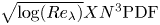 $\sqrt {\textrm{log(}R{e_\lambda }\textrm{)}} X{N^3}{\rm PDF}$, where X indicates $\varepsilon /\langle \varepsilon \rangle $ or $\varOmega /\langle \varOmega \rangle $ depending on the considered quantity. The selected threshold is 1000. This criterion was kindly suggested to us by C. Meneveau and takes into account that the histogram is evaluated on a logarithmic scale. That is, $X{N^3}{\rm PDF}$ multiplied by the logarithmic bin size represents the contribution to the histogram and the prefactor $\sqrt {\textrm{log(}R{e_\lambda }\textrm{)}} $ is due to normalization of the PDF (Meneveau & Sreenivasan Reference Meneveau and Sreenivasan1989). The rescaled histograms are shown in figure 3(c). The endpoints of the histograms are based on the highest dissipation and enstrophy values observed in the DNS. It is seen that the rescaled probability associated with the endpoints is approximately Reynolds number independent (figure 3c). Moreover, the ratio of the endpoint and the proxy for the maximum is approximately constant, which suggests that the present proxy is indeed representative for the maximum. This is shown in figure 3(d) for the enstrophy. However, the same was observed for the dissipation (not shown). In § 3.3, the proxy is used for a scaling analysis rather than the observed maximum, because it is better converged, but we should keep in mind that higher values can be encountered within the turbulent flow (figure 3).
Figure 3(d) shows that the above proxy is a better marker for the observed maximum as compared with the histogram width. However, the latter is better converged and, therefore, contains less uncertainty, which is beneficial in a scaling analysis. Moreover, the observed maximum value in a simulation (and the far tail of the PDF) may be sensitive to the numerical details, since the maximum is associated with velocity differences exceeding U over a distance corresponding to a single grid step. Here, U is the root-mean-square of the velocity fluctuations. Therefore, the grid step may play an important role in determining the highest velocity gradient that is captured, as may do the time step, the number of samples and the precision (our simulations use double precision). For this reason, any DNS result in this far tail region of the PDF remains to be validated by further experiments. Additionally, there have been some concerns raised about the validity of the Navier–Stokes equations at length scales below η (e.g. Bandak et al. Reference Bandak, Goldenfeld, Mailybaev and Eyink2022), which lengths are associated with the most extreme events. The histogram width is less prone to these potential issues. Therefore, both measures for the extrema have merit and are considered in § 3.3.
3.2. Model predictions
This section focusses on some qualitative predictions obtained from the model and highlights some limitations, which need to be understood before proceeding to the quantitative comparisons in §§ 3.3 and 3.4. The scaled model PDFs of enstrophy and dissipation, i.e. N 3PDF, are shown in figure 4 for a broad range of Reynolds numbers (black solid lines). The comparison with lognormal distributions (grey dashed lines), i.e. a model without significant shear layers, highlights the profound effect of these layers on the tails of the PDFs, and hence on the evolution of the extrema as well as the higher order moments. This is clearly visible for the histogram widths, which are given by the intersections with N 3PDF = 100. At  $R{e_\lambda } = {10^3}$, the width of the enstrophy histogram is increased twofold due to the presence of significant shear layers, whereas at $R{e_\lambda } = {10^7}$, the width is increased by four orders of magnitude due to the significant shear layers, sublayers and sub-sublayers (comparing the model with a lognormal distribution). The increase in dissipation extrema is similar, but there are some quantitative differences as discussed in § 3.3.
Model PDFs of (a) dissipation and (b) enstrophy multiplied by N 3 (black lines). Lognormal distributions at the corresponding Reynolds numbers are included for reference (grey dashed lines). Symbols (circles) mark the points corresponding to the peak contribution to the second- (red), third- (green) and fourth- (blue) order moments of each quantity. The probability threshold N 3PDF = 100 is indicated by a thin horizontal line. Its intersection with the model PDF marks the histogram width as defined in the present study.

The coloured circles in figure 4 mark the location of the peak contributions to the second-, third- and fourth-order moments. These points are in the tails of the PDFs, which means that the Reynolds number evolution of the moments is largely determined by the development of the significant shear layers (and eventually by the sublayers and sub-sublayers when they appear at very high Reynolds numbers). This is because the tail of the overall PDF is dominated by the regional PDF associated with the layers with the highest local average enstrophy and dissipation.
Another important observation concerns the peak contributions to the second-, third- and fourth-order moments relative to the histogram width. At low Reynolds number  $(R{e_\lambda } \approx {10^2})$, the fourth-order moment of the dissipation and the third- and fourth-order moments of the enstrophy receive their dominant contributions from the far tails of the PDFs beyond the histogram widths (figure 4). As commented in § 3.1, these far tails can be affected by the numerical details in a DNS and are subject to considerable uncertainty due to slow convergence (see figure 3). Consequently, the uncertainty on the fourth-order moment of the enstrophy is typically higher than that of the corresponding dissipation moment (see for example table II of Donzis et al. Reference Donzis, Yeung and Sreenivasan2008), since the former is determined by values farther beyond the histogram width. Also, the far tails in the DNS are more accurately described by a stretched exponential (e.g. Donzis et al. Reference Donzis, Yeung and Sreenivasan2008; Buaria et al. Reference Buaria, Pumir, Bodenschatz and Yeung2019) as compared with a lognormal, which is used in our model. Due to the different tail shapes, we do not expect a good match between the DNS and the present model in these cases where the moments are determined by values beyond the histogram width. In § 3.4, we make a simplistic attempt to improve the model for the prediction of the moments at low Reynolds number by truncating the model PDF. This has a similar effect as introducing a stretched exponential tail. However, these issues disappear as the Reynolds number increases. Beyond $R{e_\lambda } \approx {10^3}$, the fourth-order dissipation moment (figure 4a) and the third-order enstrophy moment (figure 4b) are determined predominantly by values below the histogram width, which is expected to yield a reliable prediction. And finally, the peak contribution to the fourth-order enstrophy moment drops below the histogram width when the Reynolds number is increased beyond $R{e_\lambda } \approx {10^4}$ (figure 4b).
At very high Reynolds number,  $R{e_\lambda }\mathrm{\ \mathbin{\lower.3ex\hbox{$\buildrel> \over {\smash{\scriptstyle\sim}\vphantom{_x}}$}}\ }{10^4}$, the model PDFs reveal local dips and bumps (figure 4). It remains uncertain whether these features are real or not, because reliable data are not yet available for the dissipation and enstrophy PDFs at $R{e_\lambda }\mathrm{\ \mathbin{\lower.3ex\hbox{$\buildrel> \over {\smash{\scriptstyle\sim}\vphantom{_x}}$}}\ }{10^4}$. Any expectation regarding the smoothness of the PDF would typically be based on an extrapolation from low-Reynolds-number results, and extrapolation is also subject to uncertainty. The bumps appear due to the assumption that all significant shear layers within the flow have exactly the same local average dissipation ${\varepsilon ^\ast }$ (and hence the same local average enstrophy). Likely, these dips and bumps will broaden and reduce in amplitude when assuming a distribution of the local average dissipation rates ${\varepsilon ^\ast }$. However, the distribution of ${\varepsilon ^\ast }$ is unknown presently and requires further study. Furthermore, the dip appears less pronounced in the enstrophy PDF as compared with the dissipation PDF, which is explained by the wider regional PDFs. This increases the overlap between the regional PDFs for the background and the significant shear layers, thereby reducing the dip. We emphasize that these local dips in the model PDF occur at relatively low magnitude, much lower than the peak contributions to the second-, third- and fourth-order moments (figure 4). Therefore, the impact of these features on the magnitude of the high-order moments is small, as was already established for the second-order dissipation moment by Elsinga et al. (Reference Elsinga, Ishihara and Hunt2020). Furthermore, in Appendix C, we present a model without dips by assuming a distribution of ${\varepsilon ^\ast }$ and confirm that this does not fundamentally alter the results as presented in §§ 3.3 and 3.4. Since the conclusions do not seem to be affected and, presently, there is little justification for the assumed distribution of ${\varepsilon ^\ast }$, we show below the results from the basic model, i.e. assuming that ${\varepsilon ^\ast }$ is the same for all significant shear layers.
3.3. Scaling of the extrema
The Reynolds number dependencies of the histogram widths are presented in figure 5. The DNS results reveal that  ${\varOmega _{width}}/\langle \varOmega \rangle > {\varepsilon _{width}}/\langle \varepsilon \rangle $, as expected since the enstrophy PDF is wider. However, the ratio of these normalized histogram widths is not constant and increases from approximately 1.5 at Reλ = 90 to 1.8 at Reλ = 1445 (see inset in figure 5a). Note that ratios are noisy quantities, because the uncertainties in the numerator and the denominator combine. The observed gradual increase of the ratio is related to a different Reynolds number scaling exponent for the enstrophy extrema as compared with the dissipation extrema, which is discussed below.
(a) Histogram width for enstrophy (red circles) and dissipation rate (blue squares) obtained from our DNS data of homogenous isotropic turbulence at seven different Reynolds numbers. The black and grey solid lines show the present model predictions for the enstrophy and dissipation, while the grey dotted line shows the prediction from the model of Luo et al. (Reference Luo, Shi and Meneveau2022) for the dissipation (exponent 1.2). The red dotted and dashed lines represent power laws with exponents 1.33 and 1.40, respectively, and the blue dotted and dashed lines represent power laws with exponents 1.13 and 1.33, respectively. These dotted lines correspond to the observed scaling at Reλ ~ 100, while the dashed lines present the observed scaling at Reλ ~ 1000. The inset shows the ratio  $({\varOmega _{width}}\langle \varepsilon \rangle)/({\varepsilon _{width}}\langle \varOmega \rangle)$ versus Reλ for our DNS. Panel (b) presents the same data and model predictions over an extended Reynolds number range. Power laws with exponents 1.3, 3/2 and 7/4 are indicated for reference.

The DNS data show that the Reynolds number scaling exponent, i.e. the slope in figure 5(a), gradually increases with Reλ and is different for each quantity. The Reynolds number scaling exponent for the histogram width of enstrophy increases slightly from approximately 1.33 to 1.40 over the present range of Reynolds numbers, i.e. Reλ = 90–1445, while the scaling exponent for the histogram width of dissipation increases from approximately 1.13 to 1.33 over the same range. Clearly, the scaling exponent for extreme dissipation is more sensitive to the Reynolds number. The uncertainty on these exponents is estimated at 0.02, which implies an uncertainty of 0.03 for the difference between the scaling exponents. The scaling exponents predicted by our model agree to within 0.05, which is consistent with the good agreement observed between the DNS and model PDFs (figure 2). At low Reynolds number (Reλ < 200), the model is found to overpredict the histogram width by approximately 10 % (see also figure 2a).
The results for the proxies of the maximum enstrophy and dissipation (figure 6a) are qualitatively consistent with those for the histogram widths (figure 5a), in that: (i) the ratio of the normalized maxima increases with Reλ; (ii) the Reynolds number scaling exponents for enstrophy and dissipation maxima are different and larger for the enstrophy and (iii) the scaling exponent for the maximum dissipation increases with increasing Reλ over the present range, which is captured by our model to within 0.05. Hence, the histogram width and the proxy of the maximum convey a similar picture, which demonstrates that the main conclusions on the scaling of the enstrophy and dissipation extrema are robust with respect to the definition used.
Maxima for enstrophy and dissipation. The meaning of the symbols and lines is identical to figure 5. However, the magnitude of the power law exponents is different. The red dotted and dashed lines represent power laws with exponents 1.63 and 1.70, respectively, while the blue dotted and dashed lines represent power laws with exponents 1.35 and 1.63, respectively. The prediction from the model by Luo et al. (Reference Luo, Shi and Meneveau2022) (grey dotted line) yields an exponent of 1.5 for the dissipation maximum. The inset in panel (a) shows the ratio  $({\varOmega _{max}}\langle \varepsilon \rangle)/({\varepsilon _{max}}\langle \varOmega \rangle)$ versus Reλ for our DNS.

However, there are slight quantitative differences between the exponents for the histogram width and those for the proxy of the maximum. The latter are larger by approximately 0.3, which is easily explained by the fact that the maxima are more extreme than the histogram widths (compare figures 5 and 6). This also explains why the uncertainty on the maxima obtained from the DNS is larger, because the PDFs are less converged for the more extreme values. Consequently, a larger scatter around the fitted power laws is observed for the maxima, and hence their fitted exponents are subject to a greater uncertainty. The scatter in the data prevents a firm conclusion on the Reynolds number dependence of the scaling exponent for the maximum enstrophy over the range considered in figure 6(a).
The traditional Kolmogorov and multifractal predictions of the scaling exponents for the extrema are clearly different from the observations at finite Reynolds number, as noted before (Buaria et al. Reference Buaria, Pumir, Bodenschatz and Yeung2019; Elsinga et al. Reference Elsinga, Ishihara and Hunt2020). In these predictions, it is assumed that the extreme velocity gradients scale with the largest velocity scale, i.e. U, and the smallest length scale in the flow. Indeed, the velocity of the most intense vortical structures was found to scale with U (e.g. Jiménez & Wray Reference Jiménez and Wray1998; Ghira et al. Reference Ghira, Elsinga and da Silva2022). The smallest length scale is given by the Kolmogorov length scale (in Kolmogorov theory) or, in the case of multifractal theory, by  ${\eta _{{h_{min}}}}\sim LRe_\lambda ^{ - 2/(1 + {h_{min}})}$ (Paladin & Vulpiani Reference Paladin and Vulpiani1987; Dubrulle Reference Dubrulle2019). Here, the minimum Hölder exponent is considered to be hmin = 0 (Paladin & Vulpiani Reference Paladin and Vulpiani1987), which is consistent with the strongest velocity gradients scaling with U. This leads to ${\varOmega _{max}}/\langle \varOmega \rangle \sim {\varepsilon _{max}}/\langle \varepsilon \rangle \sim Re_\lambda ^1$ for Kolmogorov theory and ${\varOmega _{max}}/\langle \varOmega \rangle \sim {\varepsilon _{max}}/\langle \varepsilon \rangle \sim Re_\lambda ^2$ for multifractal theory. Note that the scaling exponents are constant and that there is no distinction between dissipation and enstrophy, both scale according to the velocity gradients squared. A similar theory by Yakhot and Sreenivasan (Yakhot & Sreenivasan Reference Yakhot and Sreenivasan2005; Yakhot Reference Yakhot2006; Sreenivasan & Yakhot Reference Sreenivasan and Yakhot2021) also predicts $Re_\lambda ^2$ scaling for the maximum dissipation, as does the hierarchy of self-stretched vortex instabilities described by Jiménez & Wray (Reference Jiménez and Wray1998) for the maximum enstrophy. The Reynolds number scaling exponents of 1 and 2 are inconsistent with the present data at finite Reλ (figures 5a and 6a).
An important caveat related to the above comparison is that the theory is developed for the absolute maximum, whereas the observations concern a proxy of the maximum based on a threshold of the scaled histogram. As argued in § 3.1, the present proxy for the maximum seems to follow the maximum observed in the DNS, which suggests it represents the development of the absolute maximum, if it exists. However, for a more faithful comparison, it would be of interest to extend the above theoretical predictions to observables such as the present threshold of the scaled histogram.
Currently there are two known models that accurately predict scaling exponents for extreme dissipation over the range Reλ ≈ 100–1000. The first is our layer-based model (Elsinga et al. Reference Elsinga, Ishihara and Hunt2020), which is extended here to enstrophy (solid lines in figures 5a and 6a). The second is the multifractal intermittency model by Luo et al. (Reference Luo, Shi and Meneveau2022), which predicts constant scaling exponents (grey dotted lines in figures 5(a) and 6(a), see captions for the corresponding numerical values). These exponents were inferred from the dissipation PDFs presented in their figure 4(b). However, constant exponents do not capture the developments with the Reynolds number as observed in the DNS data. The results here and in § 3.4 suggest that the multifractal intermittency model yields the approximate average exponent over the range Reλ ≈ 100–1000. Furthermore, constant exponents cannot reconcile identical scaling of enstrophy and dissipation in the limit of infinite Reynolds number with the scaling differences observed at finite Reynolds number (see also below). In contrast, the present model captures the Reλ dependence of the scaling exponents, which, moreover, is different for dissipation and enstrophy. Other theories and models have not yet been able to explain this difference and its Reynolds number dependence. It suggests that significant shear layers are key to advancing the prediction of extreme dissipation and enstrophy.
Given its successful predictions at finite Reynolds numbers, we use the present model to examine how the significant shear layers and their (sub-) sublayers may affect the approach of an infinite Reynolds number limit. At low to moderate Reynolds numbers where DNS is available, we observe a difference in the scaling exponents for the enstrophy and dissipation extrema as discussed above. This applies to both the histogram widths and the maxima. The difference between the exponents for the enstrophy and dissipation extrema decreases between Reλ = 90 and 1445, which suggests that these quantities ultimately scale the same at infinite Reynolds number in accordance with the theoretical arguments presented by He et al. (Reference He, Chen, Kraichnan, Zhang and Zhou1998) and Nelkin (Reference Nelkin1999). The present model illustrates how this state may be approached. Indeed, the difference between the predicted scaling exponents for the enstrophy and dissipation extrema reduces as Reλ increases. In figures 5(b) and 6(b), this results in nearly parallel lines at very large Reynolds numbers. At  $R{e_\lambda }\sim {10^5}$, the difference between the predicted scaling exponents for the histogram widths is only 0.05, while the difference is approximately 0.1 for the maxima. The maxima thus converge slower to an identical scaling, as is expected. Identical scaling implies that the scaling exponent is no longer affected by the regional PDF width of a particular quantity, i.e. σ, which is different for dissipation and enstrophy. It means that, at these very large Reynolds numbers, the scaling exponents are determined by the (sub-) sublayer properties. However, at low to moderate Reynolds numbers, σ is important (yielding non-parallel lines in figures 5a and 6a). Furthermore, in the limit of infinite Reynolds number, the Reλ scaling exponents of the extrema are approximately equal to the exponent returned by multifractal theory (i.e. 2). This is consistent with the multifractal theory being strictly valid in the infinite Reynolds number limit (Dubrulle Reference Dubrulle2019; Dubrulle & Gibbon Reference Dubrulle and Gibbon2022). Hence, the present model is able to reconcile the identical scaling behaviour at infinite Reynolds number with the scaling differences observed at low to moderate Reynolds number. Furthermore, it suggests that the scaling at infinite Reynolds number is determined by the layer properties and is not affected by the specifics of the considered quantity, which have been incorporated in the parameter σ.
Small jumps in the predicted extrema can be seen when sublayers and sub-sublayers first appear in the model (solid lines in figures 5 and 6). The same is observed for the predicted moments (§ 3.4). The magnitude of these jumps is approximately 10 %, which is comparable to the accuracy mentioned above. The jumps arise because fully developed sublayers and sub-sublayers appear suddenly and we have not included a transition, which may be expected when the local Reynolds number is low. These transitions are largely unexplored and require further study. However, transitions only affect the results locally, close to the points where these sublayers and sub-sublayers first appear. Away from these points, there is no effect. Therefore, the Reynolds number trends discussed above hold.
3.4. Scaling of the moments
While the extrema are a measure for the full width of the PDF, the higher order moments provide further detail on the shape of its high-magnitude tail. The Reynolds number dependence of the dissipation and enstrophy moments is shown in figure 7. The plot presents DNS data from various sources (Kerr Reference Kerr1985; Schumacher et al. Reference Schumacher, Sreenivasan and Yakhot2007; Donzis et al. Reference Donzis, Yeung and Sreenivasan2008; Yeung et al. Reference Yeung, Donzis and Sreenivasan2012, and our DNS discussed in § 2.4). In all cases, the numerical resolution was  ${k_{max}}\eta \ge 2$. Data at lower resolution as well as the third-order moments from Yeung et al. (Reference Yeung, Donzis and Sreenivasan2012) were excluded. The latter contained relatively large uncertainties. Figure 7 shows that the results from our DNS are consistent with the data in the literature at higher resolution (e.g. Donzis et al. Reference Donzis, Yeung and Sreenivasan2008), which again confirms that the present resolution is suitable (see also § 2.4). The uncertainties in the present moments are mainly attributed to convergence. Their magnitudes can be inferred from the data scatter around the fitted power laws in figure 7. As can be seen from the (model) histograms in figure 4, the number of samples increases, and hence the level of convergence improves, with decreasing order of the moment and with increasing Reynolds number. Also, the dissipation moments are more converged as compared with their enstrophy counterparts.
Moments of (a) the dissipation and (b) the enstrophy raised to the power 1/n. Symbols show DNS data from (*) Kerr (Reference Kerr1985), (squares) Schumacher et al. (Reference Schumacher, Sreenivasan and Yakhot2007), (+) Donzis et al. (Reference Donzis, Yeung and Sreenivasan2008), (Δ) Yeung et al. (Reference Yeung, Donzis and Sreenivasan2012), (∇) Buaria & Sreenivasan (Reference Buaria and Sreenivasan2022) and (o) present (§ 2.4). Coloured solid lines show results obtained from the present model (§ 2). Note that this model is not supposed to be accurate for the fourth-order moment of dissipation and the third- and fourth-order moments of enstrophy at the present Reλ (see discussion in § 3.2). However, these results are included for completeness. The dotted and dashed lines in panel (a) present power law fits of the data at low (Reλ < 250) and moderate Reynolds numbers (400 < Reλ < 1500), respectively. The dotted lines in panel (b) show power law fits over the full Reynolds number range (Reλ < 1500). The fitted exponents are indicated. Grey solid lines indicate the scaling exponents listed in the last column of table 1, which represent the minimum of the upper bound obtained from a multifractal model.

Please note that in figure 7 and throughout this section, the Reynolds number scaling is quantified for the nth-order moment raised to the power 1/n, whose dimension is equal to that of the dissipation or the enstrophy. This is convenient when comparing the different order moments, because it prevents the highest order moment from dominating the plot. However, the obtained scaling exponents are trivially converted to those for the moments by a multiplication with n. Therefore, we do not make a distinction when discussing the scaling exponents qualitatively.
Three main observations are made from the DNS data. First, the Reynolds number scaling exponents of the dissipation moments increases beyond approximately Reλ ≈ 250 (figure 7a). The power law fits at higher Reλ (dashed lines) clearly deviate from those fitted at low Reλ (dotted lines in figure 7a). It is another evidence that the scaling exponents for the dissipation are Reynolds number dependent. Furthermore, this transition coincides with the reported changes in the small-scale structure of turbulence (Elsinga et al. Reference Elsinga, Ishihara, Goudar, da Silva and Hunt2017; Das & Girimaji Reference Das and Girimaji2019; Ghira et al. Reference Ghira, Elsinga and da Silva2022) and the broadening of the dissipation PDF due to the significant shear layer contributions (§ 2.4).
Second, the exponents of the enstrophy moments do not reveal an obvious Reynolds number dependence up to at least Reλ ≈ 1500 (figure 7b). Each enstrophy moment seems well described by a single power law (dotted lines in figure 7b), despite the fact that the tail of the enstrophy PDF changes considerably beyond Reλ ≈ 250 (§ 2.4).
Third, the enstrophy and dissipation moments do not reveal identical scaling over the present range of Reynolds numbers, i.e. the scaling exponents for the enstrophy moments are larger than the scaling exponents for the dissipation moments. The only exception is given by the second-order moments at large Reynolds number  $(R{e_\lambda }\mathrm{\ \mathbin{\lower.3ex\hbox{$\buildrel> \over {\smash{\scriptstyle\sim}\vphantom{_x}}$}}\ }400)$, where the exponents appear to be the same. This is consistent with the nearly constant ratio of the second-order moments of enstrophy and dissipation normalized by their respective means, as observed by Yeung et al. (Reference Yeung, Donzis and Sreenivasan2012) over a similar range of Reλ. Moreover, it is consistent with the intuitive expectation that the lower order moments approach identical scaling first, followed by the higher order moments, the histogram widths and eventually the maxima. It suggests that the maxima present the most critical test for observing identical scaling of dissipation and enstrophy (see also § 3.3).
Furthermore, the DNS data can be compared with some of the theories for the dissipation moments. Unfortunately, the theory for the enstrophy moments is less well developed, and therefore, the discussion is restricted to the dissipation moments. As already pointed out in § 1, the existing theories have predicted or assumed that the scaling exponents are constant, which is inconsistent with the present observations (figure 7a). Nevertheless, the predicted exponents are compared with the data to understand the Reynolds number ranges where they may apply.
The theories proposed by Yakhot & Sreenivasan (Reference Yakhot and Sreenivasan2004), Yakhot (Reference Yakhot2006) (further quantified by Schumacher et al. Reference Schumacher, Sreenivasan and Yakhot2007) and Sreenivasan & Yakhot (Reference Sreenivasan and Yakhot2021) yield nearly identical scaling exponents for the dissipation moments (table 1). Their original papers presented the exponents for the large-scale Reynolds number, ReL. The corresponding exponents for the Taylor based Reynolds number, Reλ, have been obtained using  $R{e_L}\sim Re_\lambda ^{1.8}$, which is a fit of their low-Reynolds-number DNS ( $R{e_\lambda }\mathrm{\ \mathbin{\lower.3ex\hbox{$\buildrel< \over {\smash{\scriptstyle\sim}\vphantom{_x}}$}}\ }100$, Schumacher et al. Reference Schumacher, Sreenivasan and Yakhot2007). Moreover, their exponents have been divided by the order of each moment, n, which yields the scaling exponents for the moments raised to the power 1/n as presented in table 1. When compared with the DNS (figure 7a), it is seen that their predictions are very accurate at low Reynolds numbers $(R{e_\lambda }\mathrm{\ \mathbin{\lower.3ex\hbox{$\buildrel< \over {\smash{\scriptstyle\sim}\vphantom{_x}}$}}\ }250)$. The excellent agreement in this range has been noted before (Schumacher et al. Reference Schumacher, Sreenivasan and Yakhot2007; Sreenivasan & Yakhot Reference Sreenivasan and Yakhot2021). However, at higher Reλ, the DNS data deviate and the observed scaling exponents increase well beyond the predicted values (compare dashed lines in figure 7(a) with table 1).
Theoretical predictions of the scaling exponents dn of the dissipation moments raised to the power 1/n, i.e.  ${\langle {\varepsilon ^n}\rangle ^{1/n}}/\langle \varepsilon \rangle \propto Re_\lambda ^{{d_n}}$.

Several multifractal models have been proposed in the past, which yield slightly different scaling exponents. It is not our aim to review them here. We only use the results as they appear in these papers. A multifractal cascade model, also known as the p-model, was presented by Meneveau & Sreenivasan (Reference Meneveau and Sreenivasan1987). Using the suggested parameter value (p 1 = 0.7), their predicted exponents for the velocity increments are converted to the exponents for the dissipation moments by applying Nelkin's (Reference Nelkin1990) transformation (following Johnson & Meneveau Reference Johnson and Meneveau2017, see also Frisch Reference Frisch1995). The resulting scaling exponent for  ${\langle {\varepsilon ^2}\rangle ^{1/2}}/\langle \varepsilon \rangle $ is 0.17. This value is attained in the DNS near Reλ ≈ 250. Alternatively, 0.17 may be seen as the approximate average exponent over the Reynolds number range considered in figure 7(a). The exponents for the higher order moments (table 1), especially the fourth, seem accurate at low Reynolds numbers $(R{e_\lambda }\mathrm{\ \mathbin{\lower.3ex\hbox{$\buildrel< \over {\smash{\scriptstyle\sim}\vphantom{_x}}$}}\ }250)$. A multifractal model by Nelkin (Reference Nelkin1990) also yields a scaling exponent for the second-order moments (0.19) intermediate between the values identified in the data of figure 7(a). The exponents predicted by the multifractal intermittency model (Luo et al. Reference Luo, Shi and Meneveau2022) are listed in table 1. They were inferred from the dissipation PDFs presented in their paper. The exponents are close to those obtained by combining the model of She & Leveque (Reference She and Leveque1994) with Nelkin's transformation (table 1). Again, these exponents appear to be an approximate average over the considered Reynolds number range (similar to the exponents for the extrema predicted by the multifractal intermittency model, § 3.3).
In line with the comments made by Dubrulle (Reference Dubrulle2019) and Dubrulle & Gibbon (Reference Dubrulle and Gibbon2022), the exponents predicted from the multifractal spectrum can be seen as infinite Reynolds number limits, or as the minima of the upper bounds (Gibbon Reference Gibbon2023). To estimate these bounds, we use the measured multifractal spectrum for general velocity increments as provided by Dubrulle (Reference Dubrulle2019) and assume that enstrophy and dissipation scale identically in the limit of infinite Reynolds number. Some more details are given in Appendix B. It is clear that the resulting exponents (last column of table 1) are much larger than those observed in the data (figures 7a and 7b). If indeed the enstrophy, and hence the dissipation, is to approach these limits, then the scaling exponents remain Reynolds number dependent beyond the range shown in figure 7, which is in general agreement with the expectations derived from our significant shear layer model.
The challenge is to extend the above models such that they are able to capture the observed Reynolds number dependence of the exponents. This likely requires introducing Reynolds number dependent model parameters, e.g. Reynolds number dependent intermittency exponents, fractal dimensions or fractal spectra. The question remains how to obtain and explain the Reynolds number dependence of the parameters. We suggest that significant shear layers offer such opportunity, which we illustrate below by means of our model. Furthermore, our model allows considering dissipation and enstrophy scaling simultaneously.
Using our model PDFs, the moments are obtained according to
 \begin{gather}\frac{{\langle {\varepsilon ^n}\rangle }}{{{{\langle \varepsilon \rangle }^n}}} = \int_0^{{\varepsilon _{width}}/\langle \varepsilon \rangle } {\frac{{{\varepsilon ^n}}}{{{{\langle \varepsilon \rangle }^n}}}{\rm PDF}_{model}\left( {\frac{\varepsilon }{{\langle \varepsilon \rangle }}} \right)d\left( {\frac{\varepsilon }{{\langle \varepsilon \rangle }}} \right)} ,\end{gather}
 \begin{gather}\frac{{\langle {\varOmega ^n}\rangle }}{{{{\langle \varOmega \rangle }^n}}} = \int_0^{{\varOmega _{width}}/\langle\varOmega \rangle} {\frac{{{\varOmega ^n}}}{{{{\langle \varOmega \rangle }^n}}}{\rm PDF}_{model}\left( {\frac{\varOmega }{{\langle \varOmega \rangle }}} \right)d\left( {\frac{\varOmega }{{\langle \varOmega \rangle }}} \right)} ,\end{gather}
where the integration has been truncated at the histogram width for the dissipation and enstrophy as defined in § 3.1. Truncation has a similar effect as introducing a stretched exponential tail. The latter has been shown to well represent the far tails of the actual dissipation and enstrophy PDFs (e.g. Donzis et al. Reference Donzis, Yeung and Sreenivasan2008; Buaria et al. Reference Buaria, Pumir, Bodenschatz and Yeung2019). The stretched exponentials decrease to zero much faster than the lognormal distributions used in the present model, and hence, they effectively truncate the lognormal distribution. The starting point of the stretched exponential tail is unknown at present and would need to be assumed. Therefore, replacing the lognormal far tail with a stretched exponential is equally arbitrary as defining a truncation point. We have taken the latter approach for its simplicity and because our initial goal is to get some insight as to the effect of the significant shear layers at high Reynolds numbers. Note that the histogram width was shown to approximately collapse the stretched exponential tail region (§ 3.1), and therefore the histogram width is used to truncate the integral and not the proxy of the maximum. Further note that the truncation is important only at low Reynolds numbers when the moments are strongly affected by the far tail of the PDF. At higher Reynolds numbers, the main contributions occur below the histogram width (see figure 4). Without truncation, the moments would have become constant at low Reynolds number, since, in that case, the overall model PDF is given by a single lognormal with a constant width. The results from our model are presented by the coloured solid lines in figure 7. We emphasize that the moments obtained from the DNS were computed without truncation, i.e. using the full PDF.
The present model reveals a Reynolds number dependence of the scaling exponents for the dissipation moments (figure 7a), which is consistent with the DNS data. This suggests that some relevant phenomenology has been captured and that the large-scale shear layers can explain the transition occurring at approximately Reλ ≈ 250. Furthermore, the predicted magnitudes of the moments are within 10 % of the DNS, which is consistent with the tails of the PDFs being well predicted (figure 2). However, the scaling exponents appear slightly overestimated for  $R{e_\lambda }\mathrm{\ \mathbin{\lower.3ex\hbox{$\buildrel> \over {\smash{\scriptstyle\sim}\vphantom{_x}}$}}\ }700$. The inaccuracies may be linked to the assumption that all significant shear layers have exactly the same local average dissipation ${\varepsilon ^\ast }$. This assumption has some effect on the shape of the PDF (§§ 2.4 and 3.2) and possibly on the moments. However, the general conclusion that significant shear layers provide an explanation for non-constant scaling exponents seems robust to an assumed distribution of ${\varepsilon ^\ast }$ (see Appendix C). Furthermore, the present single-valued ${\varepsilon ^\ast }$ has been determined using model parameters, α and b, whose magnitudes have been largely based on the significant shear layer observed by Ishihara et al. (Reference Ishihara, Kaneda and Hunt2013) (§ 2.3). Their observation represents an example of a particularly strong shear layer, which could explain why the scaling exponents for the extrema are slightly better predicted (§ 3.3) than those for the moments. The latter may also receive contributions from weaker shear layers. As remarked in § 3.2, the distribution of ${\varepsilon ^\ast }$ requires further study.
The model prediction of the second-order moment of enstrophy shows a nearly constant scaling exponent in approximate agreement with the data (figure 7b). That is, the changes in the exponent for the enstrophy are much smaller than those in the exponent for the dissipation. The third- and fourth-order moments of enstrophy reveal larger differences, which is explained from the fact that these moments are largely determined by values exceeding the histogram width for the enstrophy (§ 3.2).
4. Summary and conclusions
DNS data showed that the Reynolds number scaling exponents for the dissipation extrema and the dissipation moments increase with the Reynolds number. Specifically, a notable change in the exponents occurs at approximately Reλ ≈ 250. The enstrophy histogram width reveals a similar, albeit smaller, increase in its scaling exponent. However, the scaling exponents for the enstrophy moments appear to be constant over the range considered, i.e. Reλ = 50−1500. Furthermore, the exponents for the enstrophy are larger than those for the dissipation over this Reλ range. It means that enstrophy and dissipation scale differently, as has been observed before (e.g. Kerr Reference Kerr1985; Yeung et al. Reference Yeung, Donzis and Sreenivasan2012). The differences decrease with increasing Reynolds number, which is related to the fact that the scaling exponents for the dissipation increase faster with Reλ than the scaling exponents for the enstrophy.
These developments near Reλ ≈ 250 coincide with the scaling transitions previously observed for other small-scale turbulence properties and the full development of large-scale shear layers (Elsinga et al. Reference Elsinga, Ishihara, Goudar, da Silva and Hunt2017; Das & Girimaji Reference Das and Girimaji2019; Ghira et al. Reference Ghira, Elsinga and da Silva2022). Therefore, Reλ ≈ 250 marks the onset of significant changes in the turbulent structure and care should be taken when extrapolating results across this Reynolds number. The development of large-scale shear layers, also known as significant shear layers, seems particularly relevant when trying to understand the observed changes in the scaling of dissipation and enstrophy, because these layers affect intermittency. That is, the most intense dissipation and enstrophy events tend to cluster inside these layers (Ishihara et al. Reference Ishihara, Kaneda and Hunt2013; Elsinga et al. Reference Elsinga, Ishihara, Goudar, da Silva and Hunt2017). We explored the effect of the large-scale shear layers on the dissipation and enstrophy scaling using the model presented in § 2, which is an extension of our previous work (Elsinga et al. Reference Elsinga, Ishihara and Hunt2020). The model parameters associated with the properties of the layer regions, i.e. α and b, were independent of the small-scale quantity considered. However, the width of the regional enstrophy and dissipation distributions, i.e. σ in (2.3), depended on the quantity considered. This difference in the value of σ reflects that intense enstrophy and dissipation are associated with different small-scale flow structures within the same large-scale shear layer. The resulting model PDFs compared favourably with available DNS data (§ 2.4).
The dissipation and enstrophy extrema are accurately predicted by our model (§ 3.3). The scaling exponents agree with the DNS to within 0.05 and, importantly, the Reynolds number dependence of the exponents is captured over the range Reλ = 94−1445. This constituted a considerable improvement over the existing predictions by traditional multifractal and Kolmogorov-type arguments with inertial-range self-similarity assumptions, which yield a constant exponent. Furthermore, our model suggests that, as the Reynolds number increases, the scaling exponents for the enstrophy and dissipation extrema approach each other. In the limit of infinite Reynolds number, the predicted scaling exponents are identical, and hence the ratio of the maxima tends to a constant, which is consistent with theoretical arguments (He et al. Reference He, Chen, Kraichnan, Zhang and Zhou1998; Nelkin Reference Nelkin1999). It suggests that the scaling of the maxima is eventually determined by layer properties and that differences between dissipation and enstrophy, i.e. σ, do not play a role. Moreover, the scaling exponent at infinite Reynolds number is approximately equal to the multifractal prediction with hmin = 0. It is remarkable that a simple layer model yields accurate results for both the maximum dissipation and the maximum enstrophy, which, moreover, connects the observed scaling behaviours at finite Reynolds number with the expected scaling at infinite Reynolds number. This can never be achieved by theories/models predicting power laws with constant exponents. In that case, either the exponents are different for enstrophy and dissipation as observed at finite Reynolds number, or they are identical as expected for infinite Reynolds number.
Our model also captures the Reynolds number dependence of the scaling exponents for the dissipation moments over the considered Reλ range, which existing theories have not been able to do (§ 3.4), but appears to be essential for enstrophy and dissipation to scale identically in the infinite Reλ limit. However, the exponents are slightly overestimated at large Reynolds number. By comparison, the scaling exponent returned for the second-order moment of enstrophy is closer to a constant, which is again consistent with DNS observations. The predictions of the higher order moments of enstrophy are less accurate for the reasons explained in § 3.2. It seems that the maxima are more accurately predicted by the present model as compared with the moments. This could be explained by the fact that the values for the model parameters were estimated using a particularly strong realization of a significant shear layer (Ishihara et al. Reference Ishihara, Kaneda and Hunt2013). The maxima will not be affected by weaker significant shear layers, but the moments might be. The issue can be addressed by considering a distribution of layer strengths within our model. However, this requires a statistical analysis of the layers, which is not yet available.
Furthermore, the model suggests that the scaling exponents for the moments of enstrophy become Reynolds number dependent at higher Reλ (when significant shear layers break down into sublayer, sub-sublayers and so on), which is needed if the multifractal prediction with hmin = 0 is to be approached in the limit of infinite Reynolds number. Any other value of the minimum Hölder exponent, hmin, and hence the exponent predicted by multifractal theory, would require an explanation for why the velocity scale associated with extreme events is different from U (as has been observed in numerous studies to date). Presently, observational support for the existence of sublayers is unavailable, since DNS barely reaches the required Reynolds numbers. Moreover, the minimum Reynolds number required for sublayers to appear is subject to some uncertainty. However, the local Reynolds number within the significant shear layer increases with the global Reynolds number and it seems reasonable to assume that, as the local turbulence becomes more intense, the significant shear layer turbulence breaks down and develops a substructure (see also § 2.1).
The present model's relative success in predicting the Reynolds number dependencies of the scaling exponents suggests that the large-scale shear layers are key to understanding extreme dissipation and enstrophy at high Reynolds number. It warrants further study and quantification of these layers and suggests that they need to be included in some way in further modelling efforts.
The present model is applicable also to other small-scale quantities based on squared velocity gradients, as demonstrated in the Appendix. In those cases, the value of σ can be obtained from the PDF at low Reynolds number (Reλ ~ 100) before the significant shear layers develop within the flow. Then the model predicts the PDFs at higher Reynolds numbers by accounting for the effect of the significant shear layers.
Acknowledgements
We thank P.K. Yeung for interesting discussions during the EUROMECH colloquium 620 ‘Extreme dissipation and intermittency in turbulence’ (May 2021), which motivated us to extend the model to enstrophy. We are grateful to C. Meneveau for the insightful discussions on the multifractal predictions of the maxima and for providing the data presented in figure 4(b) of Luo et al. (Reference Luo, Shi and Meneveau2022) and to P. Johnson and B. Dubrulle for the helpful comments.
Funding
This work was supported in part by MEXT as the ‘Program for Promoting Researches on the Supercomputer Fugaku’ (Structure and Evolution of the Universe Unraveled by Fusion of Simulation and AI) and used the computational resources of the supercomputer Fugaku provided by the RIKEN Center for Computational Science (project ID: hp230204). T.I. was supported in part by JSPS KAKENHI (grant no. JP20H01948).
Declaration of interests
The authors report no conflict of interest.
Appendix A. Squared velocity gradients
Here, we explore further extensions of the model by considering several different combinations of squared velocity gradients. As before, the model parameters linked to the large-scale shear layers do not change and are fixed at α = 0.011 and b = 0.67. The width of the log-normal, σ, is adjusted for each combination of the squared gradients.
First, the PDF of the square of the longitudinal velocity gradient,  $A_{11}^2$, is examined, where Aij is the velocity gradient tensor. Results from DNS indicated that the high-magnitude tail of the $A_{11}^2$ PDF overlapped with that of the enstrophy PDF, when these quantities were normalized using their global averages. Therefore, the same σ is used for $A_{11}^2$ and enstrophy, i.e. σ = 1.28. The model PDF is compared with the DNS data in figure 8. Only two Reynolds numbers are presented given the similarity with enstrophy. It is seen that the high-magnitude tail is well captured by the model. However, the differences at low $A_{11}^2$ magnitude are pronounced. Clearly, the assumed lognormal distribution is a reasonable approximation for the tail (up to at least the maximum value as defined in § 3.1), but it cannot capture the full PDF. By comparison, the PDF of the transverse velocity gradient, $A_{12}^2$, is wider and better represented by σ = 1.48 (not shown).
(a,b) PDFs of the longitudinal velocity gradient squared, comparing the model with σ = 1.28 (black solid line) with a lognormal distribution (grey dashed line) and the DNS data at the corresponding Reynolds number (red solid line).

Figure 9 presents the PDFs of AijAij, where repeated indices imply summation. In this case, the model PDF uses σ = 1.12, which is intermediate between the value used for dissipation and enstrophy. Again, the high-magnitude tail of the PDF is well captured by the model. At Reλ = 170, the model and the DNS are found to slightly deviate only beyond the maximum of AijAij as defined by PDF = 100/N 3 = 0.7 × 10⁻⁵.
(a,b) PDFs of the squared norm of the velocity gradient tensor, comparing the model with σ = 1.12 (black solid line) with a lognormal distribution (grey dashed line) and the DNS data at the corresponding Reynolds number (red solid line).

Other combinations of squared velocity gradients were investigated also, such as AiiAii and AijAij with i ≠ j. The results were quite similar to those already presented. This suggests that the present model for the high-magnitude tail of the PDF is generally applicable to quantities involving squared velocity gradients.
Appendix B. Scaling exponents listed in the last column of table 1
The multifractal approach discussed and reviewed by Frisch (Reference Frisch1995), Dubrulle (Reference Dubrulle2019), Dubrulle & Gibbon (Reference Dubrulle and Gibbon2022), Kaneda et al. (Reference Kaneda, Ishihara, Morishita, Yokokawa and Uno2021) and references therein assumes that there exists a local ‘Kolmogorov’ length scale,  ${\eta _h}$, for each local Hölder exponent, h, which scales with viscosity according to ${\eta _h}/L\sim Re_L^{ - 1/(1 + h)}$ (Paladin & Vulpiani Reference Paladin and Vulpiani1987). Here, ReL = UL/ν, which scales as $R{e_L}\sim Re_\lambda ^2$ at high Reynolds number. The corresponding local ‘Kolmogorov’ velocity scale is ${u_{{\eta _h}}} = U{({\eta _h}/L)^h}$. Then, assuming that the local velocity gradients scale according to ${u_{{\eta _h}}}/{\eta _h}$ and using $\langle\varepsilon\rangle \sim {U^3}/L$, one finds for the local dissipation raised to the power n,
 \begin{equation}\frac{{{\varepsilon ^n}}}{{{{\langle \varepsilon \rangle }^n}}}\sim Re_L^{ - n}{\left( {\frac{{{\eta_h}}}{L}} \right)^{2n(h - 1)}}\sim Re_L^{ - n - 2n(h - 1)/(1 + h)}.\end{equation}
In case the intermittency can be described by a multifractal spectrum C(h), we obtain for the normalized moments (in the limit  $\nu \to 0$, Dubrulle Reference Dubrulle2019; Dubrulle & Gibbon Reference Dubrulle and Gibbon2022):
 \begin{equation}\frac{{\langle {\varepsilon ^n}\rangle }}{{{{\langle \varepsilon \rangle }^n}}}\sim Re_L^{{\chi _n}}\sim Re_\lambda ^{2{\chi _n}},\end{equation}
where
 \begin{equation}{\chi _n} ={-} n - \mathop {\min }\limits_h \left( {\frac{{2n(h - 1) + C(h)}}{{1 + h}}} \right).\end{equation}
The exponents  ${\chi _n}$ are obtained using the parabolic fit for C(h) provided by Dubrulle (Reference Dubrulle2019), which is given by
 \begin{equation}C(h) = \frac{1}{{2b}}{(h - a)^2},\quad b = 0.045,\quad a = \frac{1}{3} + \frac{{3b}}{2}.\end{equation}
Note that the empirical intermittency coefficient, b = 0.045, was obtained for general velocity increments (Dubrulle Reference Dubrulle2019). However, its value is similar to those observed for transverse velocity increments and vorticity increments (Kestener & Arneodo Reference Kestener and Arneodo2004). It can, therefore, be used to estimate the enstrophy moments following essentially the same approach as outlined above. The enstrophy moments, in the limit of infinite Reynolds number, are expected to scale identically to the dissipation moment. The predicted exponents are thus representing infinite Reynolds number limits for the dissipation moments, which seems consistent with  $\nu \to 0$ used to obtain (B2). Furthermore, the minimum value of h is taken as hmin = 0 following Paladin & Vulpiani (Reference Paladin and Vulpiani1987). The resulting exponents are presented in the last column of table 1.
Alternatively, inserting the intermittency coefficient commonly associated with longitudinal velocity increments, b = 0.025 (e.g. Kestener & Arneodo Reference Kestener and Arneodo2004), in (B4) yields exponents that are closer to those reported for the other models (table 1). However, it remains unclear how that could be made compatible with identical scaling at infinite Reynolds number if the predicted enstrophy exponents are so different. It is an open issue, which we cannot solve here.
Appendix C. A PDF model without dips and bumps
The purpose of this appendix is to show that the dips and bumps in the model PDFs (figure 4) do not significantly affect the results for the dissipation moments. The focus is on the dissipation PDF, since the dips appear most pronounced. These features are removed by introducing a distribution for the average dissipation  ${\varepsilon ^\ast }$ within the layers. Note that we do not aim to optimize this distribution to obtain an improved correspondence with the data. It is only introduced as a means to prevent dips appearing in the model PDF and to examine the effect of the dips on the dissipation moments. The main reason for not optimizing the ${\varepsilon ^\ast }$ distribution is that it introduces too many unknown variables (e.g. range and shape of the distribution), and hence uncertainties, into the model, which is not helpful when trying to understand the basic effect of significant shear layers on the dissipation scaling. As mentioned in the main text, the actual ${\varepsilon ^\ast }$ distribution is unknown presently and requires further research.
Here, the average dissipation in a layer region is assumed to be continuously distributed between the background dissipation level,  ${\varepsilon _{bg}} = b\langle \varepsilon \rangle $, and an upper bound, ${\varepsilon _{up}}$, for the significant shear layers, sublayers and sub-sublayers. These upper bounds are evaluated using the same set of equations as for the single-valued ${\varepsilon ^\ast }$ in the basic version of our model (§ 2). However, the value for the coefficient α has changed from 0.011 to 0.017, which causes ${\varepsilon _{up}}$ to be slightly larger than the single-valued ${\varepsilon ^\ast }$ before. This is to account for the fact that we now consider a distribution around the previous discrete ${\varepsilon ^\ast }$. The other parameters, i.e. b and σ, have remained the same. Then we assume a power law distribution for the average dissipation in a layer with an exponent of −2, as shown in figure 10. This represents a case where the layers of different ${\varepsilon ^\ast }$ contribute equally to the global average dissipation.
Assumed distribution for the average dissipation  ${\varepsilon ^\ast }$ within the layers.

Subsequently, the above regional distribution is convoluted with a lognormal using σ to account for the dissipation variations within each layer (similar to our existing model) and is properly normalized. Then, the regional PDFs are weighted according to the significant shear layers’, sublayers’ and sub-sublayers’ contribution to the global average dissipation and added to the background distribution as before. This yields the overall PDF, which is presented figure 11. When compared with figure 4(a), it is clear that the dips and bumps have disappeared.
Model PDFs of dissipation without dips (black solid lines). Compare with figure 4(a).

The dissipation moments resulting from the PDFs without dips and bumps are presented in figure 12 (dashed coloured lines). They are qualitatively consistent with those obtained from the original model (solid coloured lines), which featured the dips and bumps in the PDFs. Most importantly, the scaling exponents increase with the Reynolds number in both cases and also the magnitude of the predicted exponents is comparable. However, there is a difference in the magnitude of the moments. The largest difference is observed for the second moment at high Reynolds numbers and corresponds to approximately a factor two, which is consistent with our previous assessment of the dips (Elsinga et al. Reference Elsinga, Ishihara and Hunt2020). Therefore, the dips and bumps in our model (§ 2) do not affect our main conclusions regarding the Reynolds number dependence of the scaling exponents and the influence of the significant shear layers.
Effect of the dips and bumps in the model PDFs on the dissipation moments. Solid coloured lines show the original results for the model with discrete  ${\varepsilon ^\ast }$, which resulted in the dips and bumps. Dashed coloured lines present the results for the distributed ${\varepsilon ^\ast }$ case, where the dissipation PDFs do not reveal dips and bumps. Symbols and grey lines show DNS data and data fits, see caption figure 7(a).


 Open access