


1. Introduction
We study the long-time behaviour of solutions with small initial data to the viscoelastic Klein–Gordon equation on the real line:
 \begin{equation}
u_{tt} - c^2 u_{xx} - \alpha u_{txx} + f(u) = 0,
\qquad
u(x,t) \in \mathbb{R}, \, x \in \mathbb{R}, \, t \geq 0,
\end{equation}
\begin{equation}
u_{tt} - c^2 u_{xx} - \alpha u_{txx} + f(u) = 0,
\qquad
u(x,t) \in \mathbb{R}, \, x \in \mathbb{R}, \, t \geq 0,
\end{equation}where  $c \gt 0$ is the wave speed,
  $\alpha \gt 0$ is the viscosity coefficient and
  $f \colon \mathbb{R} \to \mathbb{R}$ is a smooth nonlinearity with
  $f(0) = 0$ and
  $f'(0) \gt 0$. This damped nonlinear wave equation models the dynamics of an extended one-dimensional viscoelastic medium, a so-called Kelvin–Voigt solid, which exhibits both elastic behaviour (instantaneous response to deformation) and viscous damping (dissipation of energy). Here,
  $u(x,t)$ represents the displacement of the viscoelastic solid at position
  $x$ and time
  $t$. The linear term
  $-\alpha u_{txx}$ accounts for the viscous damping,Footnote 1 while the nonlinearity
  $f(u)$ governs the material’s elastic response. Since
  $f'(0) \gt 0$, the material behaves as a stiff elastic solid near equilibrium, with
  $f(u)$ acting as a restoring force. In the absence of damping and the nonlinearity, (1.1) reduces to the standard wave equation
  $u_{tt} - c^2 u_{xx} =0$. For further background, we refer to [Reference Kawashima and Shibata26, Reference Potier-Ferry34] and references therein.
By rescaling time, space, the displacement  $u$ and the viscosity coefficient
  $\alpha \gt 0$, we can arrange for
  $f'(0) = 1$ and
  $c = 1$. This simplifies (1.1) to
 \begin{equation}
u_{tt} + u - u_{xx} - \alpha u_{txx} = N(u),
\end{equation}
\begin{equation}
u_{tt} + u - u_{xx} - \alpha u_{txx} = N(u),
\end{equation}where  $N \colon \mathbb{R} \to \mathbb{R}$ is a smooth nonlinearity with
  $N(0) = N'(0) = 0$.
In this paper, we study the impact of the nonlinearity on the long-time behaviour of solutions with small initial data. More precisely, we derive a sign condition on  $N(u)$ ensuring that solutions with small initial data to (1.1) exist for all positive times, and decay at an enhanced diffusive rate. In addition, we characterize their leading-order dynamics as
  $t \to \infty$. Notably, our result implies the nonlinear stability of the equilibrium state
  $u(x,t) = 0$ against
  $L^2$-localized perturbations. We view the present contribution as a first step towards the nonlinear stability analysis of more complex solutions such as time- or space-periodic waves.
The linearized equation
 \begin{equation}
u_{tt} + u - u_{xx} - \alpha u_{txx} = 0
\end{equation}
\begin{equation}
u_{tt} + u - u_{xx} - \alpha u_{txx} = 0
\end{equation}admits the solutions 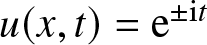 $u(x,t) = \mathrm{e}^{\pm \mathrm{i} t}$. Consequently, expressing (1.2) as an evolution system in
  $(u,u_t)$, one finds that its linearization has a continuous
  $L^2$-spectrum touching the imaginary axis at
  $\pm \mathrm{i}$, see Figure 1. Therefore, the associated semigroup exhibits at most algebraic decay rates, complicating the closure of a nonlinear iteration argument. In fact, a detailed analysis of the linear equation (1.3) in [Reference D’Abbicco and Ikehata8] shows that the optimal decay rate of its solutions is diffusive, which is typically insufficient to control quadratic or cubic nonlinearities. Indeed, all nonnegative nontrivial solutions to the nonlinear heat equation
 \begin{equation}
u_t = u_{xx} + u^p,
\end{equation}
\begin{equation}
u_t = u_{xx} + u^p,
\end{equation}with  $p = 2$ or
  $p = 3$, blow up in finite time [Reference Fujita13, Reference Hayakawa20].
Depiction of the spectrum of the operator  $\Lambda$, which consists of the half line
  $\smash{(-\infty,-\tfrac{1}{\alpha}]}$ and the intersection of the closed left-half plane with the circle with centre
  $\smash{-\tfrac{1}{\alpha}}$ and radius
  $\smash{\sqrt{1+\alpha^{-2}}}$. At frequency
  $k = 0$, the curves
  $\lambda_\pm(k)$ (depicted in red and blue) touch the imaginary axis in a quadratic tangency at the points
  $\pm \mathrm{i}$.

Nevertheless, our setting differs fundamentally from that of the nonlinear heat equation, as the touchings with the imaginary axis occur at nonzero temporal frequencies. The associated time-oscillatory behaviour of the critical modes carries over to the nonlinear terms in the variation-of-constants formula. Provided the nonlinear terms are not time-resonant, this results in oscillatory integrals with a nonstationary phase exhibiting enhanced temporal decay, which can be harnessed by integrating by parts in time, effectively following the space-time resonances method of Germain, Masmoudi and Shatah [Reference Germain15–Reference Germain, Masmoudi and Shatah18, Reference Shatah38].
Although originally developed for purely dispersive systems, the space-time resonances method has been successfully extended to dissipative settings. In [Reference de Rijk and Schneider11], it is used to establish global existence and decay of solutions with small initial data in large classes of reaction–diffusion–advection systems where components exhibit different velocities, resulting in an absence of space resonances. The present work serves as a further extension of the method to dissipative systems, where one instead exploits an absence of time resonances.Footnote 2
As explained in the expository paper [Reference Germain15], the treatment of nonlinear terms that are not time-resonant is closely related to Shatah’s normal form transform [Reference Shatah37]. The normal form transform has been adopted by Hayashi and Naumkin in [Reference Hayashi and Naumkin21–Reference Hayashi and Naumkin23] to investigate the long-term behaviour of solutions with small initial data to the Klein–Gordon equation (1.2) in the purely dispersive setting, where there is no damping ( $\alpha = 0$). Using this method, global existence and decay of small solutions is obtained for the specific nonlinearities
  $N(u) = \nu u^2$ and
  $N(u) = \nu u^3$, where
  $\nu$ is real-valued.
The current setting with viscous damping is significantly different from the one in [Reference Hayashi and Naumkin21–Reference Hayashi and Naumkin23]. Firstly, the damping term instantaneously regularizes solutions, so that we can afford to work in low regularity spaces. Secondly, at  $\alpha = 0$ the linear equation (1.2) admits the solutions
  $u(x,t) = \mathrm{e}^{\mathrm{i} (k x \pm \omega(k) t)}$ with
  $\omega(k) = \smash{\sqrt{1+k^2}}$ and
  $k \in \mathbb{R}$. As a result, the spectrum of the linearization occupies the imaginary axis, reflecting the lack of damping. For
  $\alpha \gt 0$, all frequencies but those at
  $k = 0$ are damped, which reduces the number of critical modes to two. Thus, after applying mode filters, only the occurrence of time resonances at Fourier frequency
  $0$ needs to be inspected. This enables us to handle general smooth nonlinearities. In particular, we find that a nonlinear term
  $c_n u^n$ with
  $c_n \in \mathbb{R}$ and
  $n \in \mathbb{N}_{\geq 2}$ can only be time-resonant if
  $n$ is odd. Finally, both in [Reference Hayashi and Naumkin21–Reference Hayashi and Naumkin23] and in our work, a critical resonant cubic term with coefficient
 \begin{equation}
\omega = -\frac{\mathrm{i} \left(3N'''(0) + 5 N''(0)^2\right)}{24 \pi \, \sqrt{3\alpha^2 + 1 - 2 \mathrm{i} \alpha}},
\end{equation}
\begin{equation}
\omega = -\frac{\mathrm{i} \left(3N'''(0) + 5 N''(0)^2\right)}{24 \pi \, \sqrt{3\alpha^2 + 1 - 2 \mathrm{i} \alpha}},
\end{equation}remains that cannot be handled with the space-time resonances method or normal form transform. At  $\alpha = 0$, the coefficient
  $\omega$ is purely imaginary, allowing the resonant term to be eliminated by an integrating factor with a purely imaginary phase. However, for
  $\alpha \gt 0$, the coefficient
  $\omega$ acquires a nonzero real part, complicating the analysis substantially. A refined decomposition of the solution into a Gaussian profile and a zero-mean remainder reveals that the leading-order resonant dynamics are governed by the complex separable ODE
 \begin{equation}
B'(t) = \frac{\omega}{1+t} |B(t)|^2 B(t).
\end{equation}
\begin{equation}
B'(t) = \frac{\omega}{1+t} |B(t)|^2 B(t).
\end{equation} The sign of 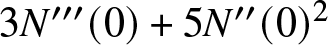 $3N'''(0) + 5 N''(0)^2$ determines the long-time behaviour: if
  $3N'''(0) + 5N''(0)^2 \lt 0$, then
  $\operatorname{Re}(\omega) \lt 0$ and all solutions to (1.6) are global and decay, giving rise to a nonlinear absorption mechanism in (1.2) that enhances diffusive decay and allows for global-in-time control of small solutions. Conversely, if
 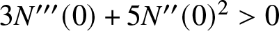 $3N'''(0) + 5 N''(0)^2 \gt 0$, then
  $\operatorname{Re}(\omega) \gt 0$ and nontrivial solutions to (1.6) blow up in finite time, implying that the resonant term obstructs the closure of a global nonlinear iteration argument. Strikingly, this shows that viscous damping may generate instabilities that are not present in the undamped Klein–Gordon equation with
  $\alpha = 0$, see Remark 1.6.
Before presenting our main results, we review existing results on the global existence of solutions to the viscoelastic Klein–Gordon equation (1.2). These results were obtained on bounded domainsFootnote 3 with the aid of energy estimates.Footnote 4 The first result [Reference Webb39] considers (1.2) for nonlinearities  $N$ for which there exists a constant
  $C \gt 0$ such that
 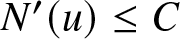 $N'(u) \leq C$ for all
  $u \in \mathbb{R}$. It asserts that solutions are global and converge to a stationary solution as
  $t \to \infty$, see also [Reference Dang Dinh Ang and Dinh9] for explicit temporal decay rates. Existence of global solutions on bounded domains in the specific case of the power-law nonlinearity
 \begin{align*}
N(u) = -\nu |u|^{p-1} u
\end{align*}
\begin{align*}
N(u) = -\nu |u|^{p-1} u
\end{align*}with  $\nu \gt 0$ and integer
  $p \geq 1$ was established in [Reference Aviles and Sandefur2]. These global solutions converge in the vanishing viscosity limit
  $\alpha \downarrow 0$ by the results in [Reference Avrin3, Reference Avrin4].
1.1. Main results
Our first result establishes global existence and enhanced diffusive decay of solutions to (1.2) with small initial data, allowing for general smooth nonlinearities  $N$ obeying the sign condition
 \begin{equation}
3N'''(0) + 5 N''(0)^2 \lt 0.
\end{equation}
\begin{equation}
3N'''(0) + 5 N''(0)^2 \lt 0.
\end{equation} Specifically, we consider initial data  $u_0 \in H^2(\mathbb{R})$ whose Fourier transform
 \begin{align*}
\hat{u}_0(k) \overset{\scriptscriptstyle{\mathrm{def}}}{=} \int_\mathbb{R} \mathrm{e}^{-\mathrm{i} k x} u(x) \, \mathrm{d} x
\end{align*}
\begin{align*}
\hat{u}_0(k) \overset{\scriptscriptstyle{\mathrm{def}}}{=} \int_\mathbb{R} \mathrm{e}^{-\mathrm{i} k x} u(x) \, \mathrm{d} x
\end{align*}lies in the Sobolev space  $W^{1,1}(\mathbb{R}) \cap W^{1,\infty}(\mathbb{R})$ and is small in that space.Footnote 5
Theorem 1.1 (Global existence and diffusive decay)
Let  $\alpha \gt 0$. Take
  $N \in C^4(\mathbb{R})$ such that
  $N(0) = 0$,
  $N'(0) = 0$ and the inequality (1.7) holds. Then, there exist positive constants
  $M_0$ and
  ${\varepsilon}$ such that, whenever
  $u_0 \in H^2(\mathbb{R})$ and
  $w_0 \in L^2(\mathbb{R})$ satisfy
  $\hat{u}_0,\hat{w}_0 \in W^{1,\infty}(\mathbb{R}) \cap W^{1,1}(\mathbb{R})$ and
 \begin{equation}
E_0 \overset{\scriptscriptstyle{\mathrm{def}}}{=} \|\hat{u}_0\|_{W^{1,1} \cap W^{1,\infty}} + \|\hat{w}_0\|_{W^{1,1} \cap W^{1,\infty}} \lt {\varepsilon},
\end{equation}
\begin{equation}
E_0 \overset{\scriptscriptstyle{\mathrm{def}}}{=} \|\hat{u}_0\|_{W^{1,1} \cap W^{1,\infty}} + \|\hat{w}_0\|_{W^{1,1} \cap W^{1,\infty}} \lt {\varepsilon},
\end{equation}there exists a unique global classical solution
 \begin{equation}
u \in C\big([0,\infty),H^2(\mathbb{R})\big) \cap C^1\big([0,\infty),L^2(\mathbb{R})\big) \cap C^1\big((0,\infty),H^2(\mathbb{R})\big) \cap C^2\big((0,\infty),L^2(\mathbb{R})\big)
\end{equation}
\begin{equation}
u \in C\big([0,\infty),H^2(\mathbb{R})\big) \cap C^1\big([0,\infty),L^2(\mathbb{R})\big) \cap C^1\big((0,\infty),H^2(\mathbb{R})\big) \cap C^2\big((0,\infty),L^2(\mathbb{R})\big)
\end{equation}of the viscoelastic Klein–Gordon equation (1.2) with initial conditions  $u(0) = u_0$ and
  $u_t(0) = w_0$, which enjoys the diffusive estimates
 \begin{equation}
\left\|u(t)\right\|_{L^\infty} \leq \frac{M_0E_0}{\sqrt{1+t}}, \qquad \left\|u(t)\right\|_{L^2} \leq \frac{M_0E_0}{(1+t)^{\frac14}}
\end{equation}
\begin{equation}
\left\|u(t)\right\|_{L^\infty} \leq \frac{M_0E_0}{\sqrt{1+t}}, \qquad \left\|u(t)\right\|_{L^2} \leq \frac{M_0E_0}{(1+t)^{\frac14}}
\end{equation}and the enhanced pointwise estimate
 \begin{equation}
\left|u(x,t)\right| \leq \frac{M_0 \, \mathrm{e}^{-\alpha \theta(x,t)}}{\sqrt{(1+t)\log(2+t)}} + \frac{M_0}{\sqrt{1+t} \, (\log(2+t))^{\frac23}}
\end{equation}
\begin{equation}
\left|u(x,t)\right| \leq \frac{M_0 \, \mathrm{e}^{-\alpha \theta(x,t)}}{\sqrt{(1+t)\log(2+t)}} + \frac{M_0}{\sqrt{1+t} \, (\log(2+t))^{\frac23}}
\end{equation}for all  $x \in \mathbb{R}$ and
  $t \geq 0$, where we denote
 \begin{equation}
\vartheta(x,t) = \frac{x^2}{2(1+\alpha^2)(1+t)}.
\end{equation}
\begin{equation}
\vartheta(x,t) = \frac{x^2}{2(1+\alpha^2)(1+t)}.
\end{equation} Theorem 1.1 establishes nonlinear asymptotic stability of the equilibrium state  $u(x,t) = 0$ in (1.2) against
  $H^2$-perturbations whose Fourier transform is small in
  $W^{1,1}(\mathbb{R}) \cap W^{1,\infty}(\mathbb{R})$. The estimate (1.10) shows that solutions to (1.1) with small initial data decay at the same rates as solutions to the heat equation
  $u_t = u_{xx}$. Identical decay rates are obtained in the purely dispersive setting (
 $\alpha = 0$) in [Reference Hayashi and Naumkin21, Reference Hayashi and Naumkin23] for the nonlinearities
  $N(u) = \nu u^p$, with
  $\nu \in \mathbb{R}$ and
  $p = 2,3$. However, the Gaussian principal part of the pointwise bound (1.11), reflecting the viscous nature of Equation (1.2), suggests that the asymptotics of the solution
  $u(x,t)$ are fundamentally different from the purely dispersive case, cf. [Reference Hayashi and Naumkin23]. This is confirmed by the next result, which determines the leading-order asymptotics under the (generic) assumption that initial data have nonzero mean. In particular, it shows that the long-time dynamics are governed by the reduced ODE (1.6).
Theorem 1.2 (Asymptotic behaviour)
Let  $\alpha \gt 0$. Let
  $N \in C^4(\mathbb{R})$ such that
  $N(0) = 0$,
  $N'(0) = 0$ and the inequality (1.7) holds. Take
  $u_* \in H^2(\mathbb{R})$ and
  $w_* \in L^2(\mathbb{R})$ with
  $\hat{u}_*,\hat{w}_* \in W^{1,\infty}(\mathbb{R}) \cap W^{1,1}(\mathbb{R})$. Suppose that
 \begin{equation}
U_* = \frac12 \int_\mathbb{R} (u_*(x) - \mathrm{i} w_*(x)) \, \mathrm{d} x
\end{equation}
\begin{equation}
U_* = \frac12 \int_\mathbb{R} (u_*(x) - \mathrm{i} w_*(x)) \, \mathrm{d} x
\end{equation}is non-zero. Then, there exist positive constants  $M_0$ and
  $\delta_0$ such that for all
  $\delta \in (0,\delta_0)$ there exists a unique global classical solution
  $u(t)$ with regularity (1.9) to the viscoelastic Klein–Gordon equation (1.2) with initial conditions
  $u(0) = \delta u_*$ and
  $u_t(0) = \delta w_*$, which obeys the estimate
 \begin{equation}
\begin{aligned}
&\sup_{x \in \mathbb{R}} \left|u(x,t) - \frac{r(t)\, \mathrm{e}^{-\alpha \vartheta(x,t)}
}{\sqrt{\pi (1+\alpha^2) (1+t)}} \operatorname{Re}\left(\sqrt{2\alpha + 2\mathrm{i}} \, \mathrm{e}^{\mathrm{i} \left(t + \psi(t) - \theta(x,t)\right)}\right)\right| \leq \frac{M_0}{\sqrt{1+t} \, (\log(2+t))^{\frac23}}
\end{aligned}
\end{equation}
\begin{equation}
\begin{aligned}
&\sup_{x \in \mathbb{R}} \left|u(x,t) - \frac{r(t)\, \mathrm{e}^{-\alpha \vartheta(x,t)}
}{\sqrt{\pi (1+\alpha^2) (1+t)}} \operatorname{Re}\left(\sqrt{2\alpha + 2\mathrm{i}} \, \mathrm{e}^{\mathrm{i} \left(t + \psi(t) - \theta(x,t)\right)}\right)\right| \leq \frac{M_0}{\sqrt{1+t} \, (\log(2+t))^{\frac23}}
\end{aligned}
\end{equation}for all  $t \geq 0$, where
  $\vartheta(x,t)$ is given by (1.12),
  $r \colon [0,\infty) \to (0,\infty)$ and
  $\psi \colon [0,\infty) \to \mathbb{R}$ are continuously differentiable functions satisfying
 \begin{equation}
\begin{aligned}
\left|r(t) - \tilde{r}(t)\right| &\leq M_0 \delta \tilde{r}(t),\\ \left|\psi(t) - \tilde{\psi}(t)\right| &\leq M_0 \delta \left(1 + |\tilde{\psi}(t)|\right),\\
\left|r(0) - \delta |U_*|\right| &\leq M_0\delta^2, \\
\left|\psi(0) - \arg(U_*)\right| &\leq M_0\delta
\end{aligned}
\end{equation}
\begin{equation}
\begin{aligned}
\left|r(t) - \tilde{r}(t)\right| &\leq M_0 \delta \tilde{r}(t),\\ \left|\psi(t) - \tilde{\psi}(t)\right| &\leq M_0 \delta \left(1 + |\tilde{\psi}(t)|\right),\\
\left|r(0) - \delta |U_*|\right| &\leq M_0\delta^2, \\
\left|\psi(0) - \arg(U_*)\right| &\leq M_0\delta
\end{aligned}
\end{equation}for  $t \geq 0$, and
  $B(t) = \tilde{r}(t) \mathrm{e}^{\mathrm{i} \tilde{\psi}(t)}$ solves the reduced ODE (1.6) with initial condition
  $B(0) = r(0)\mathrm{e}^{\mathrm{i} \psi(0)}$ and its radius and phase are explicitly given by
 \begin{equation}
\begin{aligned}
\tilde{r}(t) &= \frac{r(0)}{\sqrt{1-2\operatorname{Re}(\omega) r(0)^2 \log(1+t)}},\\
\tilde{\psi}(t) &= \psi(0) - \frac{\operatorname{Im}(\omega)\log(1-2 \operatorname{Re}(\omega) r(0)^2 \log (1+t))}{2 \operatorname{Re}(\omega)}.
\end{aligned}
\end{equation}
\begin{equation}
\begin{aligned}
\tilde{r}(t) &= \frac{r(0)}{\sqrt{1-2\operatorname{Re}(\omega) r(0)^2 \log(1+t)}},\\
\tilde{\psi}(t) &= \psi(0) - \frac{\operatorname{Im}(\omega)\log(1-2 \operatorname{Re}(\omega) r(0)^2 \log (1+t))}{2 \operatorname{Re}(\omega)}.
\end{aligned}
\end{equation} Theorem 1.2 shows that, provided the nonlinearity satisfies the sign condition (1.7), and the initial data have nonvanishing complex mean  $U_*$, the leading-order asymptotics of the solution
  $u(x,t)$ to (1.2) are governed by a spatiotemporally oscillating Gaussian profile, which decays at the enhanced diffusive rate
  $\smash{(t \log(t))^{-\frac12}}$. The oscillating Gaussian profile originates from the linearized dynamics (1.3) of the viscous Klein–Gordon equation. In contrast, the logarithmic corrections
  $r(t)$ and
  $\psi(t)$ to the amplitude and phase in (1.14) arise from the nonlinear reduced dynamics, given by the complex separable ODE (1.6). We refer to Remark 1.5 for further details. Finally, we note that the nonvanishing of the complex mean
  $U_*$ ensures that
  $\tilde{r}(t)$ is nonzero, so that (1.14)–(1.15) indeed provides a leading-order approximation of the solution
  $u(x,t)$.
If the nonlinearity does not satisfy the sign condition (1.7), then the critical resonant term obstructs the closure of a global nonlinear iteration argument. However, since the quadratic terms are not time-resonant and can be eliminated, we are still able to establish existence and diffusive decay on time intervals that are exponentially large with respect to the size of the initial data.
Theorem 1.3 (Existence and diffusive decay on exponentially long time scales)
Let  $\alpha \gt 0$. Take
  $N \in C^4(\mathbb{R})$ such that
  $N(0) = 0$ and
  $N'(0) = 0$. Then, there exist positive constants
  $M_0$ and
  ${\varepsilon}$ such that, whenever
  $u_0 \in H^2(\mathbb{R})$ and
  $w_0 \in L^2(\mathbb{R})$ satisfy
  $\hat{u}_0, \hat{w}_0 \in L^1(\mathbb{R}) \cap L^\infty(\mathbb{R})$ and
 \begin{equation}
E_0 \overset{\scriptscriptstyle{\mathrm{def}}}{=} \|\hat{u}_0\|_{L^1 \cap L^\infty} + \|\hat{w}_0\|_{L^1 \cap L^\infty} \lt {\varepsilon},
\end{equation}
\begin{equation}
E_0 \overset{\scriptscriptstyle{\mathrm{def}}}{=} \|\hat{u}_0\|_{L^1 \cap L^\infty} + \|\hat{w}_0\|_{L^1 \cap L^\infty} \lt {\varepsilon},
\end{equation}there exists a unique classical solution
 \begin{align*}
u &\in C\big([0,T_{\varepsilon}],H^2(\mathbb{R})\big) \cap C^1\big([0,T_{\varepsilon}],L^2(\mathbb{R})\big) \cap C^1\big((0,T_{\varepsilon}],H^2(\mathbb{R})\big) \cap C^2\big((0,T_{\varepsilon}],L^2(\mathbb{R})\big)
\end{align*}
\begin{align*}
u &\in C\big([0,T_{\varepsilon}],H^2(\mathbb{R})\big) \cap C^1\big([0,T_{\varepsilon}],L^2(\mathbb{R})\big) \cap C^1\big((0,T_{\varepsilon}],H^2(\mathbb{R})\big) \cap C^2\big((0,T_{\varepsilon}],L^2(\mathbb{R})\big)
\end{align*}of the viscoelastic Klein–Gordon equation (1.2) on an interval of length
 \begin{align*}
T_\varepsilon \overset{\scriptscriptstyle{\mathrm{def}}}{=} \mathrm{e}^{{\varepsilon}/E_0}-2
\end{align*}
\begin{align*}
T_\varepsilon \overset{\scriptscriptstyle{\mathrm{def}}}{=} \mathrm{e}^{{\varepsilon}/E_0}-2
\end{align*}with initial data  $u(0) = u_0$ and
  $u_t(0) = w_0$. Moreover,
  $u(t)$ obeys the diffusive estimates
 \begin{align*}
\left\|u(t)\right\|_{L^\infty} \leq \frac{M_0E_0}{\sqrt{1+t}}, \qquad \left\|u(t)\right\|_{L^2} \leq \frac{M_0E_0}{(1+t)^{\frac14}}
\end{align*}
\begin{align*}
\left\|u(t)\right\|_{L^\infty} \leq \frac{M_0E_0}{\sqrt{1+t}}, \qquad \left\|u(t)\right\|_{L^2} \leq \frac{M_0E_0}{(1+t)^{\frac14}}
\end{align*}for all  $t \in [0,T_{\varepsilon}]$.
A result similar to Theorem 1.3 holds for the nonlinear heat equation (1.4) with cubic nonlinearity ( $p=3$). Specifically, it is shown in [Reference Lee and Wei-Ming29, Theorem 3.21] and [Reference Schneider and Uecker35, Theorem 2.1] that solutions with initial data of size
  $E_0$ in
  $L^1(\mathbb{R}) \cap L^\infty(\mathbb{R})$ exist and decay diffusively on time intervals that are exponentially long in
  $E_0$. In contrast, in case of a quadratic nonlinearity (
 $p=2$), solutions to (1.4) with small initial data of size
  $E_0$ in
  $L^1(\mathbb{R}) \cap L^\infty(\mathbb{R})$ can blow up within time
  $\leq CE_0^{-2}$, where
  $C \gt 0$ is some
  $E_0$-independent constant, cf. [Reference Lee and Wei-Ming29, Theorem 3.15].
The question of whether solutions exhibit blow-up when (1.7) is not satisfied remains open. In the viscous regime with  $\alpha \gt 0$, we do not expect solutions to preserve compact support, which complicates the adaptation of known blow-up results [Reference Delort12, Reference Keel and Tao27]. Nevertheless, as discussed in Remark 1.6, we expect that the failure of (1.7) leads to the instability of the rest state
  $u(x,t) = 0$ in (1.2).
Remark 1.4. Another approach to obtaining global existence of solutions with small initial data is to consider so-called transparent nonlinearities [Reference Lannes28], which vanish at resonant frequencies, thereby eliminating the singularity that typically arises when integrating by parts. For the Klein–Gordon equation, known transparent terms involve a spatial derivative [Reference Katayama25, Reference Moriyama32]. Our analysis shows that the critical quadratic and cubic terms in (1.2) are not transparent. However, in case 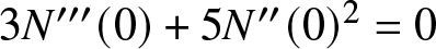 $3N'''(0) + 5 N''(0)^2 = 0$, the coefficient in front of the critical remaining resonant term vanishes, and we expect that Theorem 1.3 can be extended to a global result. We leave this boundary case as an open question for future research.
Remark 1.5. We explain how the approximation (1.14) of the leading-order asymptotics in Theorem 1.2 can be formally derived from the linearized viscous Klein–Gordon equation (1.3) and the nonlinear reduced ODE (1.6). Introducing the auxiliary variable  $z = u_t$, Equation (1.3) can be written as the linear hyperbolic–parabolic system
 \begin{equation}
Z_t = \mathcal{A} Z, \qquad \mathcal{A} \overset{\scriptscriptstyle{\mathrm{def}}}{=} \begin{pmatrix} 0 & 1 \\ \partial_x^2 - 1 & \alpha \partial_x^2\end{pmatrix},
\end{equation}
\begin{equation}
Z_t = \mathcal{A} Z, \qquad \mathcal{A} \overset{\scriptscriptstyle{\mathrm{def}}}{=} \begin{pmatrix} 0 & 1 \\ \partial_x^2 - 1 & \alpha \partial_x^2\end{pmatrix},
\end{equation}in  $Z = (u,z)^\top$. The Fourier symbol
  $\widehat{\mathcal{A}}(k)$ of the differential operator
  $\mathcal{A}$ possesses the eigenvalues
 \begin{equation}
\lambda_{\pm}(k) = -\dfrac{1}{2}\alpha k^2 \pm \mu(k), \qquad \mu(k) = \sqrt{\dfrac{1}{4}\alpha^2k^4 - 1 - k^2}, \qquad k \in \mathbb{R}.
\end{equation}
\begin{equation}
\lambda_{\pm}(k) = -\dfrac{1}{2}\alpha k^2 \pm \mu(k), \qquad \mu(k) = \sqrt{\dfrac{1}{4}\alpha^2k^4 - 1 - k^2}, \qquad k \in \mathbb{R}.
\end{equation} Hence,  $\widehat{\mathcal{A}}(k)$ is diagonalizable for
  $|k| \ll 1$ and it holds
 \begin{equation}
\mathcal{A}(k) = S(k)^{-1} \mathrm{diag}(\lambda_+(k), \lambda_-(k)) S(k),
\end{equation}
\begin{equation}
\mathcal{A}(k) = S(k)^{-1} \mathrm{diag}(\lambda_+(k), \lambda_-(k)) S(k),
\end{equation}where  $S(k)$ is an invertible matrix with
 \begin{align*}
S(0) = \frac{1}{\sqrt{2}}\begin{pmatrix} 1 & -1 \\ \mathrm{i} & \mathrm{i}\end{pmatrix}, \qquad S(0)^{-1} = \frac{1}{\sqrt{2}}\begin{pmatrix} 1 & -\mathrm{i} \\ -1 & -\mathrm{i}\end{pmatrix}.
\end{align*}
\begin{align*}
S(0) = \frac{1}{\sqrt{2}}\begin{pmatrix} 1 & -1 \\ \mathrm{i} & \mathrm{i}\end{pmatrix}, \qquad S(0)^{-1} = \frac{1}{\sqrt{2}}\begin{pmatrix} 1 & -\mathrm{i} \\ -1 & -\mathrm{i}\end{pmatrix}.
\end{align*} Since high frequencies are exponentially damped, see §4, only the low frequencies contribute to the leading-order asymptotics. Thus, assuming that the diagonalization (1.20) holds for all  $k \in \mathbb{R}$, solutions of
 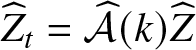 $\widehat{Z}_t = \widehat{\mathcal{A}}(k)\widehat{Z}$ with initial condition
  $\widehat{Z}(0) = \widehat{Z}_0$ are given by
 \begin{align*}
\widehat{Z}(k,t)
= S(k)^{-1}
\mathrm{diag}\bigl(\mathrm{e}^{\lambda_+(k)(1+t)}, \mathrm{e}^{\lambda_-(k)(1+t)}\bigr)
\mathrm{diag}\bigl(\mathrm{e}^{-\lambda_+(k)}, \mathrm{e}^{-\lambda_-(k)}\bigr)
S(k)\,\widehat{Z}_0(k).
\end{align*}
\begin{align*}
\widehat{Z}(k,t)
= S(k)^{-1}
\mathrm{diag}\bigl(\mathrm{e}^{\lambda_+(k)(1+t)}, \mathrm{e}^{\lambda_-(k)(1+t)}\bigr)
\mathrm{diag}\bigl(\mathrm{e}^{-\lambda_+(k)}, \mathrm{e}^{-\lambda_-(k)}\bigr)
S(k)\,\widehat{Z}_0(k).
\end{align*}Letting
 \begin{equation}
\tilde{\lambda}_\pm(k) = \pm \mathrm{i} + \frac{1}{2}\left(-\alpha \pm \mathrm{i}\right) k^2
\end{equation}
\begin{equation}
\tilde{\lambda}_\pm(k) = \pm \mathrm{i} + \frac{1}{2}\left(-\alpha \pm \mathrm{i}\right) k^2
\end{equation}be the quadratic approximants of the eigenvalues  $\lambda_\pm(k)$, we then identify
 \begin{equation}
S(0)^{-1} \mathrm{diag}\left(\mathrm{e}^{\tilde{\lambda}_+(k) (1+t)}, \mathrm{e}^{\tilde{\lambda}_-(k) (1+t)} \right) \mathrm{diag}\left(\mathrm{e}^{-\lambda_+(0)}, \mathrm{e}^{-\lambda_-(0)} \right) S(0) \widehat{Z}_0(0)
\end{equation}
\begin{equation}
S(0)^{-1} \mathrm{diag}\left(\mathrm{e}^{\tilde{\lambda}_+(k) (1+t)}, \mathrm{e}^{\tilde{\lambda}_-(k) (1+t)} \right) \mathrm{diag}\left(\mathrm{e}^{-\lambda_+(0)}, \mathrm{e}^{-\lambda_-(0)} \right) S(0) \widehat{Z}_0(0)
\end{equation}as the leading-order part of 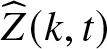 $\widehat{Z}(k,t)$. Applying the inverse Fourier transform, the first component of (1.22) provides an approximation of solutions to the linearized equation (1.3). Taking initial conditions
  $u(0) = \delta u_*$ and
  $u_t(0) = \delta w_*$, this approximation is explicitly given by
 \begin{equation}
\begin{aligned}
u(x,t) &= \operatorname{Re} \left(\mathcal{F}^{-1}\left(\mathrm{e}^{\tilde{\lambda}_+(\cdot) (1+t) - \tilde{\lambda}_+(0)}\right)\right) \delta \hat{u}_*(0) = \operatorname{Re} \left(\frac{\sqrt{\alpha + \mathrm{i}} \, \mathrm{e}^{\mathrm{i} t - \frac{(\alpha + \mathrm{i}) x^2}{2(1 + \alpha^2) (1+t)}}}{\sqrt{2\pi(1 + \alpha^2)(1+t)}}\right) \int_\mathbb{R} \delta u_*(x) \mathrm{d} x\\
&= \frac{\mathrm{e}^{-\alpha \vartheta(x,t)} }{\sqrt{\pi(1 + \alpha^2)(1+t)}} \operatorname{Re}\left(\sqrt{2\alpha + 2\mathrm{i}} \, \mathrm{e}^{\mathrm{i} \left(t - \theta(x,t)\right)}\right) \operatorname{Re}(\delta U_*),
\end{aligned}
\end{equation}
\begin{equation}
\begin{aligned}
u(x,t) &= \operatorname{Re} \left(\mathcal{F}^{-1}\left(\mathrm{e}^{\tilde{\lambda}_+(\cdot) (1+t) - \tilde{\lambda}_+(0)}\right)\right) \delta \hat{u}_*(0) = \operatorname{Re} \left(\frac{\sqrt{\alpha + \mathrm{i}} \, \mathrm{e}^{\mathrm{i} t - \frac{(\alpha + \mathrm{i}) x^2}{2(1 + \alpha^2) (1+t)}}}{\sqrt{2\pi(1 + \alpha^2)(1+t)}}\right) \int_\mathbb{R} \delta u_*(x) \mathrm{d} x\\
&= \frac{\mathrm{e}^{-\alpha \vartheta(x,t)} }{\sqrt{\pi(1 + \alpha^2)(1+t)}} \operatorname{Re}\left(\sqrt{2\alpha + 2\mathrm{i}} \, \mathrm{e}^{\mathrm{i} \left(t - \theta(x,t)\right)}\right) \operatorname{Re}(\delta U_*),
\end{aligned}
\end{equation}where  $U_*$ is as in (1.13) and
  $\vartheta(x,t)$ is given by (1.12). We refer to (11.38) for more details on the computation of
  $\smash{\mathcal{F}^{-1} (\mathrm{e}^{\tilde{\lambda}_+(\cdot) (1+t)})}$.
The nonlinear approximation (1.14) in Theorem 1.2 is then obtained from the linear approximation (1.23) by modulating the phase and amplitude with  $\tilde{\psi}(t)$ and
  $\tilde{r}(t)$, respectively, where
  $B(t) = \tilde{r}(t) \mathrm{e}^{\mathrm{i}\tilde{\phi}(t)}$ solves the nonlinear reduced ODE (1.6) with initial condition
  $B(0) = \delta U_*$. This contributes an additional logarithmic decay factor, which arises because the sign condition (1.7) guarantees that the cubic term in (1.6) is of absorption type. Such logarithmic corrections to the leading-order linear asymptotics have also been identified in other dissipative problems such as the cubic heat equation
  $u_t = u_{xx} - \smash{u^3}$ with absorption, cf. [Reference Galaktionov, Kurdyumov and Samarskiuı14].
Beyond the framework developed here, another approach to systematically capture nonlinear corrections to the leading-order linear asymptotics is the renormalization group method [Reference Bricmont and Kupiainen5, Reference Bricmont, Kupiainen and Lin6]. An interesting direction for future research would be to explore whether the renormalization group method can be adapted to the dispersive-dissipative setting of the viscous Klein–Gordon equation considered here.
1.2. Technical summary
In this section, we provide an outline of our analysis, which eventually leads to the proofs of Theorems 1.1, 1.2 and 1.3. The main idea is to eliminate nonresonant critical terms using the space-time resonances method and arrive at a reduced nonlinear ordinary differential equation governing the leading-order dynamics of solutions to (1.2) with small initial data. The reduction process involves several steps that we summarize below.
We start by recasting Equation (1.2) as a first-order system in time. Using the change of variable
 \begin{equation*}
U =
\begin{pmatrix}
u \\ \big(1-\partial_{x}^2\big)^{-1}\big(u_t - \frac{\alpha}{2} u_{xx}\big)
\end{pmatrix}
\end{equation*}
\begin{equation*}
U =
\begin{pmatrix}
u \\ \big(1-\partial_{x}^2\big)^{-1}\big(u_t - \frac{\alpha}{2} u_{xx}\big)
\end{pmatrix}
\end{equation*}whose components have balanced regularity, we arrive at a system of the form
 \begin{equation}
U_t = \Lambda U + \mathcal{N}_2(U) + \mathcal{N}_3(U) + \mathcal{R}(U).
\end{equation}
\begin{equation}
U_t = \Lambda U + \mathcal{N}_2(U) + \mathcal{N}_3(U) + \mathcal{R}(U).
\end{equation} Here, the linear operator  $\Lambda$ is sectorial, and has a spectrum that touches the imaginary axis in a quadratic tangency at
  $\pm \mathrm{i}$, see Figures 1 and 2. This indicates that the semigroup
  $\mathrm{e}^{\Lambda t}$ obeys the same diffusive estimates as the heat semigroup:
  $\left\lVert\smash{\mathrm{e}^{\partial_x^2 t}}\right\rVert_{L^p \to L^\infty} \leq C t^{-1/(2p)}$,
  $1 \leq p \leq \infty$. The quadratic and cubic terms,
  $\mathcal{N}_2(U)$ and
  $\mathcal{N}_3(U)$, pose the main challenge in proving global existence, whereas the residual term
  $\mathcal{R}(U)$ is at least quartic in
  $U$ and thus irrelevant for the long-time dynamics. Indeed, proving the global existence of small solutions via the mild formulation
 \begin{equation*}
U(t) = \mathrm{e}^{\Lambda t} U_0 + \int_0^t \mathrm{e}^{\Lambda (t - \tau)} \big(\mathcal{N}_2(U) + \mathcal{N}_3(U) + \mathcal{R}(U) \big)(\tau) \, \mathrm{d} \tau
\end{equation*}
\begin{equation*}
U(t) = \mathrm{e}^{\Lambda t} U_0 + \int_0^t \mathrm{e}^{\Lambda (t - \tau)} \big(\mathcal{N}_2(U) + \mathcal{N}_3(U) + \mathcal{R}(U) \big)(\tau) \, \mathrm{d} \tau
\end{equation*}of (1.24) through  $L^1$-
 $L^\infty$-estimates is only possible if the cumulative nonlinear effects remain integrable over time, cf. [Reference Schneider and Uecker36, Section 14]. Given the aforementioned diffusive temporal decay rates, quadratic and cubic nonlinear terms are critical, while the decay rates associated with quartic or higher-order terms are integrable in time.
Depiction of the real (solid) and imaginary (dashed) parts of the spectral curves  $\lambda_\pm(k)$ as a function of the spatial frequency
  $k$. Left: plot of
  $\lambda_+(k)$, corresponding to the red curve in Figure 1. Right: plot of
  $\lambda_-(k)$, corresponding to the blue curve in Figure 1. At frequency
  $k=0$, the real parts of
  $\lambda_\pm(k)$ vanish quadratically.

Our first step in analysing the dynamics of (1.24) is to decompose the solution into low- and high-frequency components in order to distinguish between critical oscillatory modes and exponentially damped ones. Writing  $\widehat{U} = \widehat{U}_\mathrm{c} + \widehat{U}_\mathrm{s} = \chi \widehat{U} + (1-\chi) \widehat{U}$, where
  $\chi$ is a cut-off function centred at the origin, we see that problematic nonlinear terms are low-frequency interactions only. That is, the dynamics in Fourier space is given by
 \begin{equation*}
\begin{cases}
\partial_t \widehat{U}_\mathrm{c} = \widehat{\Lambda} \widehat{U}_\mathrm{c} + \chi \widehat{\mathcal{N}}_2(\widehat{U}_\mathrm{c}) + \chi \widehat{\mathcal{N}}_3(\widehat{U}_\mathrm{c}) + \mathcal{E}_1,\\
\partial_t \widehat{U}_\mathrm{s} = \widehat{\Lambda} \widehat{U}_\mathrm{s} + \mathcal{E}_2.
\end{cases}
\end{equation*}
\begin{equation*}
\begin{cases}
\partial_t \widehat{U}_\mathrm{c} = \widehat{\Lambda} \widehat{U}_\mathrm{c} + \chi \widehat{\mathcal{N}}_2(\widehat{U}_\mathrm{c}) + \chi \widehat{\mathcal{N}}_3(\widehat{U}_\mathrm{c}) + \mathcal{E}_1,\\
\partial_t \widehat{U}_\mathrm{s} = \widehat{\Lambda} \widehat{U}_\mathrm{s} + \mathcal{E}_2.
\end{cases}
\end{equation*}where all terms denoted by  $\mathcal{E}$, here and in the following, represent irrelevant nonlinear terms that do not affect the long-time behaviour of solutions with small initial data. Next, we introduce a near-identity change of variables
 \begin{equation}
V = \widehat{U}_\mathrm{c} + K_2(\widehat{U}_\mathrm{c}) + K_3(\widehat{U}_\mathrm{c}),
\end{equation}
\begin{equation}
V = \widehat{U}_\mathrm{c} + K_2(\widehat{U}_\mathrm{c}) + K_3(\widehat{U}_\mathrm{c}),
\end{equation}for the critical low-frequency component, where  $K_2(\widehat{U}_\mathrm{c})$ is quadratic in
  $\widehat{U}_\mathrm{c}$ and
  $K_3(\widehat{U}_\mathrm{c})$ is cubic in
  $\widehat{U}_\mathrm{c}$. This normal form transformation is invertible and designed to remove all quadratic terms and all non-resonant cubic terms, leading to the evolution equation
 \begin{equation*}
V_t = \widehat{\Lambda} V + Q_{\mathrm{res}}(V) + \mathcal{E}_3,
\end{equation*}
\begin{equation*}
V_t = \widehat{\Lambda} V + Q_{\mathrm{res}}(V) + \mathcal{E}_3,
\end{equation*}where  $Q_{\mathrm{res}}(V)$ is a resonant cubic term. The transformation (1.25) arises from the space-time resonances method by integrating by parts in time. At this stage, we can already establish existence and diffusive decay of small solutions on exponentially long time scales, as in [Reference Moriyama, Tonegawa and Tsutsumi33], leading to the proof of Theorem 1.3.
The proofs of Theorems 1.1 and 1.2 require a final reduction step in which we identify the leading-order behaviour of  $V$ as a diffusive Gaussian profile
  $\hat{g}$ with a complex-valued amplitude
  $A$. Proceeding as in [Reference de Rijk and Schneider10, Theorem 1.5], we write
 \begin{equation*} V(t,k) = A(t) \hat{g}(t, k) + \hat{\rho}(t,k), \end{equation*}
where  $\hat{\rho}$ denotes a residual term exhibiting higher-order decay. We arrive at an evolution system of the form
 \begin{equation*}
\begin{cases} \partial_t \hat{\rho} = \widehat{\Lambda} \hat{\rho} + \mathcal{E}_4, \\ r'(t) = \frac{\operatorname{Re}(\omega)}{1+t} r(t)^3 + \mathcal{E}_5,
\end{cases}
\end{equation*}
\begin{equation*}
\begin{cases} \partial_t \hat{\rho} = \widehat{\Lambda} \hat{\rho} + \mathcal{E}_4, \\ r'(t) = \frac{\operatorname{Re}(\omega)}{1+t} r(t)^3 + \mathcal{E}_5,
\end{cases}
\end{equation*}for  $r = \lvert A\rvert$ and
  $\hat{\rho}$. The sign of
  $\operatorname{Re}(\omega)$ governs the long-time behaviour of the ODE for
  $r(t)$. In particular, if the sign condition (1.7) holds, then we find
  $\operatorname{Re}(\omega) \lt 0$ and solutions exist globally in time. Exploiting this, we are able to close a global nonlinear iteration argument and prove Theorems 1.1 and 1.2.
Remark 1.6. If  $\operatorname{Re}(\omega) \gt 0$, then all solutions to the separable ODE (1.6) with initial data
  $B(0) = B_0 \in \mathbb{C} \setminus \{0\}$ blow up at
  $t_0 = \smash{\mathrm{e}^{1/(2 \operatorname{Re}(\omega) |B_0|^2)}-1}$. This suggests, as in the nonlinear heat equation (1.4) with
  $p = 3$, cf. [Reference Hayakawa20, Reference Lee and Wei-Ming29], that the rest state
  $u(x,t) = 0$ in (1.2) is unstable if
  $3N'''(0) + 5 N''(0)^2 \gt 0$, with the instability only manifesting itself on exponentially long time scales.
Remark 1.7. Upon introducing the auxiliary variable  $z = u_t$, Equation (1.2) can be rewritten as the hyperbolic–parabolic system
 \begin{equation}
Z_t = \mathcal{A} Z +
\begin{pmatrix}
0 \\ N(u)
\end{pmatrix}
\end{equation}
\begin{equation}
Z_t = \mathcal{A} Z +
\begin{pmatrix}
0 \\ N(u)
\end{pmatrix}
\end{equation}in  $Z = (u,z)^\top$, where the linear operator
  $\mathcal{A}$ is defined in (1.18). The long-time dynamics of hyperbolic–parabolic systems of conservation laws have been studied extensively; see [Reference Liu and Zeng30] and references therein. As in (1.26), such systems of conservation laws possess critical diffusive modes at spatial frequency
  $k=0$, while modes at nonzero frequencies are exponentially damped. However, an important difference with the present setting concerns both the nature of the critical modes and the structure of the nonlinearity. Here, the critical modes are time-oscillatory and the nonlinearity is not of divergence form. Consequently, the mechanism leading to additional temporal decay differs from that in hyperbolic–parabolic systems of conservation laws. In our case, additional temporal decay is generated by the time-oscillatory behaviour of nonresonant nonlinear terms, whereas in [Reference Liu and Zeng30], additional decay arises from differences in group velocities between critical modes and a spatial derivative acting on the nonlinearity. As in our approach, the pointwise Green’s function method developed in [Reference Liu and Zeng30] allows one to extract the leading-order asymptotics of solutions with small initial data. It would be an interesting direction for future research to investigate whether such Green’s function techniques could also be successfully applied to system (1.26).
1.3. Organization
In §2, we introduce some notation and define the function spaces in which we consider the solutions to (1.2). Section 3 is devoted to the local existence analysis of solutions to (1.2). In §4, we study the linear dynamics of (1.2). Subsequently, in §5, we apply mode filters to (1.2), which separate low-frequency from high-frequency modes. In §6, we isolate the critical quadratic and cubic terms and estimate the irrelevant residual terms. We eliminate the quadratic and nonresonant cubic terms with the aid of the space-time resonances method in §7 and §8, respectively. Section 9 contains estimates on the resonant cubic terms, whereas in §10 we analyse the reduced system governing the leading-order dynamics. Finally, we close the nonlinear iteration argument in §11, which finishes the proofs of Theorems 1.1, 1.2 and 1.3.
2. Notation and function spaces
In this section, we introduce some notation and define the function spaces in which we construct solutions to the viscoelastic Klein–Gordon equation (1.2).
First of all, given a set  $S$ and maps
  $A, B \colon S \to \mathbb{R}$, we write ‘
 $A(x) \lesssim B(x)$ for
  $x \in S$’ to express that there exists a constant
  $C \gt 0$, independent of
  $x$, such that
  $A(x) \leq CB(x)$ holds for all
  $x \in S$.
Secondly, we employ the nonunitary Fourier transform  $\mathcal{F} \colon L^2(\mathbb{R}) \to L^2(\mathbb{R})$ and its inverse
  $\mathcal{F}^{-1} \colon L^2(\mathbb{R}) \to L^2(\mathbb{R})$ throughout this paper. They are determined by their action on the dense subspace
  $L^1(\mathbb{R}) \cap L^2(\mathbb{R})$ of
  $L^2(\mathbb{R})$, which is given by
 \begin{align*}
\mathcal{F}(u)(k) = \int_\mathbb{R} \mathrm{e}^{-\mathrm{i} k x} u(x) \mathrm{d} x, \qquad \mathcal{F}^{-1}(v)(k) = \frac{1}{2\pi} \int_\mathbb{R} \mathrm{e}^{\mathrm{i} k x} v(k) \mathrm{d} k.
\end{align*}
\begin{align*}
\mathcal{F}(u)(k) = \int_\mathbb{R} \mathrm{e}^{-\mathrm{i} k x} u(x) \mathrm{d} x, \qquad \mathcal{F}^{-1}(v)(k) = \frac{1}{2\pi} \int_\mathbb{R} \mathrm{e}^{\mathrm{i} k x} v(k) \mathrm{d} k.
\end{align*} As usual, we abbreviate  $\hat{u} = \mathcal{F}(u)$.
Next, we introduce the algebraically weighted  $L^2$-space
 \begin{align*}
L^2_1(\mathbb{R}) = \left\{f \in L^2(\mathbb{R}) : \rho f \in L^2(\mathbb{R})\right\},
\end{align*}
\begin{align*}
L^2_1(\mathbb{R}) = \left\{f \in L^2(\mathbb{R}) : \rho f \in L^2(\mathbb{R})\right\},
\end{align*}where  $\rho \colon \mathbb{R} \to \mathbb{R}$ is the weight
  $\rho(k) = \sqrt{1+k^2}$. We equip
  $L^2_1(\mathbb{R})$ with the norm
  $\smash{\|f\|_{L^2_1}} = \smash{\|\rho f\|_{L^2}}$. It is well-known that the Fourier transform maps
  $L^2_1(\mathbb{R})$ isomorphically onto
  $H^1(\mathbb{R})$. Moreover, we define the Banach spaces
 \begin{align*}
Y_m &= \big\{f \in L^2(\mathbb{R}) : \rho^m \hat{f} \in L^1(\mathbb{R}) \cap L^\infty(\mathbb{R})\big\},\\
X_m &= \big\{f \in L_1^2(\mathbb{R}) : \rho^m \hat{f}, \rho^m \hat{f}' \in L^1(\mathbb{R}) \cap L^\infty(\mathbb{R})\big\},
\end{align*}
\begin{align*}
Y_m &= \big\{f \in L^2(\mathbb{R}) : \rho^m \hat{f} \in L^1(\mathbb{R}) \cap L^\infty(\mathbb{R})\big\},\\
X_m &= \big\{f \in L_1^2(\mathbb{R}) : \rho^m \hat{f}, \rho^m \hat{f}' \in L^1(\mathbb{R}) \cap L^\infty(\mathbb{R})\big\},
\end{align*}for  $m \in \mathbb N_0$, by their norms
 \begin{align*}
\|f\|_{Y_m} &= \big\|\rho^m \hat{f}\big\|_{L^1} + \big\|\rho^m \hat{f}\big\|_{L^\infty},\\
\|f\|_{X_m} &= \big\|\rho^m \hat{f}\big\|_{L^1} + \big\|\rho^m \hat{f}\big\|_{L^\infty} + \big\|\rho^m \hat{f}'\big\|_{L^1} + \big\|\rho^m \hat{f}'\big\|_{L^\infty},
\end{align*}
\begin{align*}
\|f\|_{Y_m} &= \big\|\rho^m \hat{f}\big\|_{L^1} + \big\|\rho^m \hat{f}\big\|_{L^\infty},\\
\|f\|_{X_m} &= \big\|\rho^m \hat{f}\big\|_{L^1} + \big\|\rho^m \hat{f}\big\|_{L^\infty} + \big\|\rho^m \hat{f}'\big\|_{L^1} + \big\|\rho^m \hat{f}'\big\|_{L^\infty},
\end{align*}respectively. For  $m \in \mathbb N_0$, we have the continuous embeddings
 \begin{align*}
W^{m,1}(\mathbb{R}) \cap W^{m,\infty}(\mathbb{R}) \hookrightarrow Y_m \hookrightarrow H^m(\mathbb{R}) \cap W^{m,\infty}(\mathbb{R}),
\end{align*}
\begin{align*}
W^{m,1}(\mathbb{R}) \cap W^{m,\infty}(\mathbb{R}) \hookrightarrow Y_m \hookrightarrow H^m(\mathbb{R}) \cap W^{m,\infty}(\mathbb{R}),
\end{align*}and, similarly,
 \begin{align*}
&\left\{f \in L^2(\mathbb{R}) : f, \rho f \in W^{m,1}(\mathbb{R}) \cap W^{m,\infty}(\mathbb{R})\right\} \\
&\qquad \ \hookrightarrow X_m \hookrightarrow \left\{f \in L^2(\mathbb{R}) : f, \rho f \in H^m(\mathbb{R}) \cap W^{m,\infty}(\mathbb{R})\right\}.
\end{align*}
\begin{align*}
&\left\{f \in L^2(\mathbb{R}) : f, \rho f \in W^{m,1}(\mathbb{R}) \cap W^{m,\infty}(\mathbb{R})\right\} \\
&\qquad \ \hookrightarrow X_m \hookrightarrow \left\{f \in L^2(\mathbb{R}) : f, \rho f \in H^m(\mathbb{R}) \cap W^{m,\infty}(\mathbb{R})\right\}.
\end{align*}3. Local existence and uniqueness
We write the viscoelastic Klein–Gordon equation (1.2) as a semilinear evolution problem by introducing the tailor-made variable
 \begin{equation}
v = \left(1-\partial_x^2\right)^{-1} \left(u_t - \frac{\alpha}{2} u_{xx}\right).
\end{equation}
\begin{equation}
v = \left(1-\partial_x^2\right)^{-1} \left(u_t - \frac{\alpha}{2} u_{xx}\right).
\end{equation}Thus, we obtain the system
 \begin{equation}
U_t = \Lambda U + \mathcal{N}(U),
\end{equation}
\begin{equation}
U_t = \Lambda U + \mathcal{N}(U),
\end{equation}in  $U = (u,v)^\top$, where the linear operator
  $\Lambda$ is given by
 \begin{align*}
\Lambda = \begin{pmatrix} \frac{\alpha}{2} \partial_x^2 & 1-\partial_x^2 \\ -1 + \frac{\alpha^2}{4} \partial_x^4 \left(1-\partial_x^2\right)^{-1} & \frac{\alpha}{2} \partial_x^2\end{pmatrix},
\end{align*}
\begin{align*}
\Lambda = \begin{pmatrix} \frac{\alpha}{2} \partial_x^2 & 1-\partial_x^2 \\ -1 + \frac{\alpha^2}{4} \partial_x^4 \left(1-\partial_x^2\right)^{-1} & \frac{\alpha}{2} \partial_x^2\end{pmatrix},
\end{align*}and the nonlinearity  $\mathcal{N}(U)$ is defined by
 \begin{align*}
\mathcal{N}(U) = \left(1-\partial_x^2\right)^{-1} N\left(U_1\right) \mathbf{e}_2,
\end{align*}
\begin{align*}
\mathcal{N}(U) = \left(1-\partial_x^2\right)^{-1} N\left(U_1\right) \mathbf{e}_2,
\end{align*}where  $\mathbf{e}_2$ is the unit vector
  $\mathbf{e}_2 = (0, 1)^\top$ and
  $U_1$ denotes the first coordinate of the vector
  $U$.
$U$.
We will establish that the linear operator  $\Lambda$ in (3.2) is sectorial on the spaces
  $Y_0$ and
  $L^2(\mathbb{R})$, implying that (3.2) is a semilinear parabolic problem. We note that this is a direct consequence of the viscous dissipation, modelled by the term
  $-\alpha u_{txx}$ in (1.2). Thus, standard parabolic semigroup theory [Reference Lunardi31] yields local existence of a maximal mild solution to (3.2) in the spaces
  $X_0$ and
  $Y_0$, required for the proof of Theorems 1.1, 1.2 and 1.3, respectively, as well as in the space
  $L^2(\mathbb{R})$. In the subsequent result we then show, under the additional regularity assumption
  $u(0) \in H^2(\mathbb{R})$, that, if
  $U(t) = (u(t),v(t))^\top$ is a mild solution in
  $L^2(\mathbb{R})$ of system (3.2), then its first coordinate
  $u(t)$ is a classical solution of the viscoelastic Klein–Gordon equation (1.2).
Remark 3.1. It is well-known [Reference Ikehata, Todorova and Yordanov24, Reference Webb39] that the linear operator  $\mathcal{A}$, given by (1.18), generates a
  $C^0$-semigroup on the space
  $H^1(\mathbb{R}) \times L^2(\mathbb{R})$ and an analytic semigroup on the space
  $H^2(\mathbb{R}) \times L^2(\mathbb{R})$. These facts are used in the upcoming Proposition 3.3. The disadvantage of the first-order formulation (1.26) with respect to (3.2) is that the components of the vector
  $Z = (u,z)^\top$ do not have the same regularity in the spaces
  $H^1(\mathbb{R}) \times L^2(\mathbb{R})$ and
  $H^2(\mathbb{R}) \times L^2(\mathbb{R})$, which is avoided by the preconditioner
  $(1-\partial_x^2)^{-1}$ in (3.1). Moreover, the preconditioner induces additional localization on the nonlinearity in (3.2) in Fourier space. For these reasons, we adopt the first-order formulation (3.2) in our nonlinear analysis.
We prove local existence of a maximal mild solution to (3.2) in one of the spaces  $X_0, Y_0$ or
  $L^2(\mathbb{R})$.
Proposition 3.2. Let  $\mathcal{X}$ be one of the spaces
  $X_0$,
  $Y_0$ or
  $L^2(\mathbb{R})$. Let
  $U_0 \in \mathcal{X}$. Then, there exist
  $T_{\max} \in (0,\infty]$ and a unique, maximally defined, mild solution
  $U \in C\big([0,T_{\max}),\mathcal{X}\big)$ of (3.2) with initial condition
  $U(0) = U_0$. If
  $T_{\max} \lt \infty$, then it holds
 \begin{equation}
\limsup_{t \uparrow T_{\max}} \|U(t)\|_{\mathcal{X}} = \infty.
\end{equation}
\begin{equation}
\limsup_{t \uparrow T_{\max}} \|U(t)\|_{\mathcal{X}} = \infty.
\end{equation}Proof. We first consider the cases  $\mathcal{X} = Y_0$ or
  $\mathcal{X} = L^2(\mathbb{R})$. Let
  $Z_m$ denote either the space
  $Y_m$ or
  $H^m(\mathbb{R})$ for
  $m \in \mathbb{N}_0$. We show that
  $\Lambda$ is a sectorial operator on
  $Z_0$ and
  $\mathcal{N}$ is a locally Lipschitz continuous nonlinearity on
  $Z_0$. Then, the existence of a maximal mild solution to (3.2) follows from standard semigroup theory for semilinear parabolic problems.
We observe that the elliptic operator  $\partial_x^2$ acts on
  $Z_0$ with dense domain
  $Z_2$. Thus, the preconditioner
  $(1-\partial_x^2)^{-1}$ is a bounded linear operator from
  $Z_0$ into
  $Z_2$. We aim to show that
  $\Lambda$ is a sectorial operator on
  $Z_0$ by regarding
  $\Lambda$ as a bounded perturbation of the operator
  $\Lambda_0$ given by
 \begin{align*}
\Lambda_0 = \begin{pmatrix} \frac{\alpha}{2} \partial_x^2 & 1-\partial_x^2 \\ \frac{\alpha^2}{4} \partial_x^4 \left(1-\partial_x^2\right)^{-1} & \frac{\alpha}{2} \partial_x^2\end{pmatrix}.
\end{align*}
\begin{align*}
\Lambda_0 = \begin{pmatrix} \frac{\alpha}{2} \partial_x^2 & 1-\partial_x^2 \\ \frac{\alpha^2}{4} \partial_x^4 \left(1-\partial_x^2\right)^{-1} & \frac{\alpha}{2} \partial_x^2\end{pmatrix}.
\end{align*} The spectrum of the constant-coefficient operator  $\Lambda_0$ is determined by the eigenvalues
 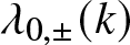 $\lambda_{0,\pm}(k)$ of its Fourier symbol
 \begin{align*} \widehat{\Lambda}_0(k) = \begin{pmatrix} -\frac{\alpha}{2} k^2 & 1+k^2 \\ \frac{\alpha^2}{4} \frac{k^4}{1+k^2} &- \frac{\alpha}{2} k^2\end{pmatrix},
\end{align*}
\begin{align*} \widehat{\Lambda}_0(k) = \begin{pmatrix} -\frac{\alpha}{2} k^2 & 1+k^2 \\ \frac{\alpha^2}{4} \frac{k^4}{1+k^2} &- \frac{\alpha}{2} k^2\end{pmatrix},
\end{align*}which are given by
 \begin{align*}
\lambda_{0,-}(k) = -\alpha k^2, \qquad \lambda_{0,+}(k) = 0.
\end{align*}
\begin{align*}
\lambda_{0,-}(k) = -\alpha k^2, \qquad \lambda_{0,+}(k) = 0.
\end{align*} In particular, for  $k \in \mathbb{R} \setminus \{0\}$, the matrix
  $\hat{\Lambda}_0(k)$ is diagonalizable. For later use, we note that the associated change of basis is represented by a matrix
  $S(k)$, whose columns are comprised of the eigenvectors of
  $\hat{\Lambda}_0(k)$, and its inverse, which are given by
 \begin{align*}
S(k) = \begin{pmatrix}
\frac{2 \left(k^2+1\right)}{\alpha k^2} & -\frac{2
\left(k^2+1\right)}{\alpha k^2} \\
1 & 1
\end{pmatrix}, \qquad S(k)^{-1} = \begin{pmatrix}
\frac{\alpha k^2}{4 k^2+4} & \frac{1}{2} \\
-\frac{\alpha k^2}{4 k^2+4} & \frac{1}{2}
\end{pmatrix},
\end{align*}
\begin{align*}
S(k) = \begin{pmatrix}
\frac{2 \left(k^2+1\right)}{\alpha k^2} & -\frac{2
\left(k^2+1\right)}{\alpha k^2} \\
1 & 1
\end{pmatrix}, \qquad S(k)^{-1} = \begin{pmatrix}
\frac{\alpha k^2}{4 k^2+4} & \frac{1}{2} \\
-\frac{\alpha k^2}{4 k^2+4} & \frac{1}{2}
\end{pmatrix},
\end{align*}for  $k \in \mathbb{R} \setminus \{0\}$. That is, we have
  $S(k)^{-1} \hat{\Lambda}_0(k) S(k) = \mathrm{diag}(0,-\alpha k^2)$ for
  $k \in \mathbb{R} \setminus \{0\}$. One readily observes that the coefficients of
  $S(\cdot)$ and
  $S(\cdot)^{-1}$ are bounded on
  $\mathbb{R} \setminus (-1,1)$.
Thus, we find 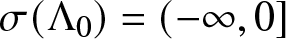 $\sigma(\Lambda_0) = (-\infty,0]$. So, the resolvent set
  $\rho(\Lambda_0)$ contains the sector
  $\Sigma_0 = \{\lambda \in \mathbb{C} : \lambda \neq 1, |\mathrm{arg}(\lambda - 1)| \leq \frac{3\pi}{4}\}$. The resolvent
  $(\Lambda_0 - \lambda)^{-1}$ possesses the Fourier symbol
 \begin{align*}
\frac{1}{\lambda}\begin{pmatrix}
-1 + \frac{\alpha k^2}{2(\alpha k^2 + \lambda)} & -\frac{1+k^2}{\alpha k^2 + \lambda} \\
-\frac{\alpha^2 k^4}{4\left(1+k^2\right)\left(\alpha k^2 + \lambda\right)} & -1 + \frac{\alpha k^2}{2(\alpha k^2 + \lambda)}
\end{pmatrix},
\end{align*}
\begin{align*}
\frac{1}{\lambda}\begin{pmatrix}
-1 + \frac{\alpha k^2}{2(\alpha k^2 + \lambda)} & -\frac{1+k^2}{\alpha k^2 + \lambda} \\
-\frac{\alpha^2 k^4}{4\left(1+k^2\right)\left(\alpha k^2 + \lambda\right)} & -1 + \frac{\alpha k^2}{2(\alpha k^2 + \lambda)}
\end{pmatrix},
\end{align*}for  $\lambda \in \Sigma_0$. For
  $\lambda \in \Sigma_0$ and
  $k \in \mathbb{R}$, we have the basic inequalities
 \begin{align*}
\left|1 + \frac{\lambda}{\alpha k^2}\right| \geq \frac{1}{\sqrt{2}}, \quad \ \ \left|\alpha k^2 + \lambda\right| \geq \frac{1}{\sqrt{2}}, \quad\ \ \frac{k^2}{1+k^2} \leq 1, \quad\ \ |\lambda - 1| \leq |\lambda| + 1 \leq |\lambda|(1+\sqrt{2}).
\end{align*}
\begin{align*}
\left|1 + \frac{\lambda}{\alpha k^2}\right| \geq \frac{1}{\sqrt{2}}, \quad \ \ \left|\alpha k^2 + \lambda\right| \geq \frac{1}{\sqrt{2}}, \quad\ \ \frac{k^2}{1+k^2} \leq 1, \quad\ \ |\lambda - 1| \leq |\lambda| + 1 \leq |\lambda|(1+\sqrt{2}).
\end{align*} Hence, there exists a constant  $M \gt 0$ such that
 \begin{align*} \left\|(\Lambda_0 - \lambda)^{-1}\right\|_{Y_0} \leq \frac{M}{|\lambda - 1|},
\end{align*}
\begin{align*} \left\|(\Lambda_0 - \lambda)^{-1}\right\|_{Y_0} \leq \frac{M}{|\lambda - 1|},
\end{align*}for all  $\lambda \in \Sigma_0$. We conclude that
  $\Lambda_0$ is a sectorial operator on
  $Z_0$. By standard perturbation theory of sectorial operators [Reference Lunardi31, Proposition 2.4.1], it follows that
  $\Lambda$ is a sectorial operator on
  $Z_0$, since
  $\Lambda$ is a bounded perturbation of
  $\Lambda_0$. In addition, since the domain
  $D(\Lambda) = \{U \in Z_0 : \Lambda U \in Z_0\}$ obviously contains the dense subspace
  $C_c^\infty(\mathbb{R}) \subset Z_0$ of all test functions,
  $\Lambda$ is densely defined.
Furthermore,  $\mathcal{N}$ is locally Lipschitz continuous on
  $Z_0$, because
  $N$ is smooth, the space
  $Z_1$ continuously embeds into
  $L^\infty(\mathbb{R})$ and
  $\smash{(1-\partial_x^2)^{-1}}$ is a bounded linear operator from
  $Z_0$ into
  $Z_2$. Combining the latter with the fact that
  $\Lambda$ is sectorial and densely defined on
  $Z_0$, it follows by standard local existence theory [Reference Lunardi31, Theorem 7.1.2 and Proposition 7.1.7] for semilinear parabolic equations that there exist
  $T_{\max} \in (0,\infty]$ and a unique, maximally defined, mild solution
  $U \in C\big([0,T_{\max}),Z_0\big)$ of (3.2) with initial condition
  $U(0) = U_0$. If
  $T_{\max} \lt \infty$, then we have (3.3). This establishes the result for the case
  $\mathcal{X} = Y_0$ or
  $\mathcal{X} = L^2(\mathbb{R})$.
Next, we consider the case  $\mathcal{X} = X_0$. We introduce the tailor made variable
  $V = x U$ and observe that
  $(U,V)$ satisfies the four-component system
 \begin{equation}
\begin{aligned}
U_t &= \Lambda U + \mathcal{N}(U),\\
V_t &= \Lambda V + \widetilde{\Lambda} U + \widetilde{\mathcal{N}}(U,V)
\end{aligned}
\end{equation}
\begin{equation}
\begin{aligned}
U_t &= \Lambda U + \mathcal{N}(U),\\
V_t &= \Lambda V + \widetilde{\Lambda} U + \widetilde{\mathcal{N}}(U,V)
\end{aligned}
\end{equation}where  $\widetilde{\Lambda}$ is the linear operator with Fourier symbol
 \begin{align*}
\mathrm{i} \hat{\Lambda}'(k) = \begin{pmatrix} -\alpha \mathrm{i} k & 2\mathrm{i} k \\ \frac{\alpha^2 k^3\left(2+k^2\right)}{2\left(1+k^2\right)^2} & -\alpha \mathrm{i} k
\end{pmatrix},
\end{align*}
\begin{align*}
\mathrm{i} \hat{\Lambda}'(k) = \begin{pmatrix} -\alpha \mathrm{i} k & 2\mathrm{i} k \\ \frac{\alpha^2 k^3\left(2+k^2\right)}{2\left(1+k^2\right)^2} & -\alpha \mathrm{i} k
\end{pmatrix},
\end{align*}and we denote
 \begin{align*}
\widetilde{\mathcal{N}}(U,V) = \left(1-\partial_x^2\right)^{-1}\left(V_1\frac{N(U_1)}{U_1} \mathbf{e}_2\right) - 2 \partial_x \left(1-\partial_x^2\right)^{-2}\left(N(U_1) \mathbf{e}_2\right).
\end{align*}
\begin{align*}
\widetilde{\mathcal{N}}(U,V) = \left(1-\partial_x^2\right)^{-1}\left(V_1\frac{N(U_1)}{U_1} \mathbf{e}_2\right) - 2 \partial_x \left(1-\partial_x^2\right)^{-2}\left(N(U_1) \mathbf{e}_2\right).
\end{align*} Since  $\Lambda$ is sectorial and densely defined on
  $Y_0$, the operator
  $\mathcal{L}$ on the product space
  $Y_0 \times Y_0$ given by
  $(U,V) \mapsto (\Lambda U, \Lambda V)$ is also sectorial and densely defined. Next, we show that, for any
  $\epsilon \gt 0$, the operator
  $(U,V) \mapsto (0,\widetilde{\Lambda}U)$ is relatively bounded with respect to
  $\mathcal{L}$ with
  $\mathcal{L}$-bound
  $\epsilon \gt 0$. Firstly, we compute
 \begin{align*}
S(k)^{-1} \hat{\Lambda}'(k) S(k) = \begin{pmatrix}
0 & -\frac{\alpha k}{k^2+1} \\
\frac{\alpha k}{k^2+1} & -2 \alpha k \\
\end{pmatrix},
\end{align*}
\begin{align*}
S(k)^{-1} \hat{\Lambda}'(k) S(k) = \begin{pmatrix}
0 & -\frac{\alpha k}{k^2+1} \\
\frac{\alpha k}{k^2+1} & -2 \alpha k \\
\end{pmatrix},
\end{align*}for  $k \in \mathbb{R} \setminus \{0\}$. Hence, abbreviating
  $S(k)^{-1} W = (w_1,w_2)$ and using that
  $S(\cdot)$,
  $S(\cdot)^{-1}$ and
  $k \mapsto k/(1+k^2)$ are bounded on
  $\mathbb{R} \setminus (-1,1)$, we establish
 \begin{align*}
\left|\hat{\Lambda}'(k) W\right| &\leq \left|S(k)\right| \left|S(k)^{-1} \hat{\Lambda}'(k) S(k) S(k)^{-1} W\right| \lesssim |k| \left|w_2\right| + \left|S(k)^{-1} W\right|\\
&\lesssim \left|S(k)^{-1} \hat{\Lambda}_0(k) S(k) S(k)^{-1} W\right|^{\frac12} \left|S(k)^{-1} W\right|^{\frac12} + \left|S(k)^{-1}\right| \left|W\right| \\
&\lesssim \left|S(k)^{-1}\right| \left|\hat{\Lambda}_0(k) W\right|^{\frac12} \left|W\right|^{\frac12} + \left|S(k)^{-1}\right| \left|W\right|\\
&\lesssim \left|\hat{\Lambda}_0(k) W\right|^{\frac12} \left|W\right|^{\frac12} + \left|W\right| \lesssim \left|\hat{\Lambda}(k) W\right|^{\frac12} \left|W\right|^{\frac12} + \left|W\right|,
\end{align*}
\begin{align*}
\left|\hat{\Lambda}'(k) W\right| &\leq \left|S(k)\right| \left|S(k)^{-1} \hat{\Lambda}'(k) S(k) S(k)^{-1} W\right| \lesssim |k| \left|w_2\right| + \left|S(k)^{-1} W\right|\\
&\lesssim \left|S(k)^{-1} \hat{\Lambda}_0(k) S(k) S(k)^{-1} W\right|^{\frac12} \left|S(k)^{-1} W\right|^{\frac12} + \left|S(k)^{-1}\right| \left|W\right| \\
&\lesssim \left|S(k)^{-1}\right| \left|\hat{\Lambda}_0(k) W\right|^{\frac12} \left|W\right|^{\frac12} + \left|S(k)^{-1}\right| \left|W\right|\\
&\lesssim \left|\hat{\Lambda}_0(k) W\right|^{\frac12} \left|W\right|^{\frac12} + \left|W\right| \lesssim \left|\hat{\Lambda}(k) W\right|^{\frac12} \left|W\right|^{\frac12} + \left|W\right|,
\end{align*}for  $W \in \mathbb{C}^2$ and
  $k \in \mathbb{R} \setminus (-1,1)$. Combining the latter with the fact that
  $\hat{\Lambda}'(\cdot)$ is bounded on
  $[-1,1]$, we obtain
 \begin{equation}
\begin{aligned}
\left|\hat{\Lambda}'(k) W\right|\lesssim \left|\hat{\Lambda}(k) W\right|^{\frac12} \left|W\right|^{\frac12} + \left|W\right|,
\end{aligned}
\end{equation}
\begin{equation}
\begin{aligned}
\left|\hat{\Lambda}'(k) W\right|\lesssim \left|\hat{\Lambda}(k) W\right|^{\frac12} \left|W\right|^{\frac12} + \left|W\right|,
\end{aligned}
\end{equation}for all  $W \in \mathbb{C}^2$ and
  $k \in \mathbb{R}$. Thus, by employing Young’s inequality we infer that, for any
  $\epsilon \gt 0$, the operator
  $\widetilde{\Lambda}$ is relatively bounded with respect to
  $\Lambda$ with
  $\Lambda$-bound
  $\epsilon$. Consequently, for any
  $\epsilon \gt 0$, the operator
  $(U,V) \mapsto (0,\widetilde{\Lambda}U)$ is relatively bounded with respect to
  $\mathcal{L}$ with
  $\mathcal{L}$-bound
  $\epsilon \gt 0$. So, it follows by [Reference Lunardi31, Proposition 2.4.2] that
 \begin{align*}
\begin{pmatrix}
U \\ V
\end{pmatrix} \mapsto \begin{pmatrix}
\Lambda U \\ \Lambda V + \widetilde{\Lambda} U
\end{pmatrix},
\end{align*}
\begin{align*}
\begin{pmatrix}
U \\ V
\end{pmatrix} \mapsto \begin{pmatrix}
\Lambda U \\ \Lambda V + \widetilde{\Lambda} U
\end{pmatrix},
\end{align*}is a sectorial and densely defined operator on  $Y_0 \times Y_0$ and, thus, generates an analytic semigroup on
  $Y_0 \times Y_0$.
Next, we note that  $\widetilde{\mathcal{N}} \colon Y_0 \times Y_0 \to Y_0$ is locally Lipschitz continuous, since the map
  $u \mapsto N(u)/u$ is smooth and because
  $\partial_x (1-\partial_x^2)^{-2}$ and
  $(1-\partial_x^2)^{-1}$ are bounded linear operators on
  $Y_0$. We conclude that
 \begin{align*}
\begin{pmatrix}
U \\ V
\end{pmatrix} \mapsto \begin{pmatrix}
\mathcal{N}(U) \\ \widetilde{\mathcal{N}}(U,V)
\end{pmatrix}
\end{align*}
\begin{align*}
\begin{pmatrix}
U \\ V
\end{pmatrix} \mapsto \begin{pmatrix}
\mathcal{N}(U) \\ \widetilde{\mathcal{N}}(U,V)
\end{pmatrix}
\end{align*}is locally Lipschitz continuous on  $Y_0 \times Y_0$. It follows again by [Reference Lunardi31, Theorem 7.1.2 and Proposition 7.1.7] that there exist
  $T_{\max} \in (0,\infty]$ and a unique, maximally defined, mild solution
 \begin{align*}
\begin{pmatrix}U \\ V \end{pmatrix} \in C\big([0,T_{\max}),Y_0 \times Y_0\big),
\end{align*}
\begin{align*}
\begin{pmatrix}U \\ V \end{pmatrix} \in C\big([0,T_{\max}),Y_0 \times Y_0\big),
\end{align*}of (3.4) with initial condition  $U(0) = (U_0,V_0)^\top$, where
  $V_0(x) = x U_0(x)$. If
  $T_{\max} \lt \infty$, then it holds
 \begin{align*}
\limsup_{t \uparrow T_{\max}} \|(U(t),V(t))\|_{Y_0 \times Y_0} = \infty.
\end{align*}
\begin{align*}
\limsup_{t \uparrow T_{\max}} \|(U(t),V(t))\|_{Y_0 \times Y_0} = \infty.
\end{align*} Upon recalling  $V(x,t) = x U(x,t)$, we conclude that
  $U \in C\big([0,T_{\max}),X_0\big)$ is a solution of (3.2) with initial condition
  $U(0) = U_0$. Moreover, if
  $T_{\max} \lt \infty$, then we have (3.3).
The next result relates the mild solution  $U(t)$ of (3.2), established in Proposition 3.2, to a classical solution of the viscoelastic Klein–Gordon equation (1.2) under the additional regularity assumption that
  $u_0 \in H^2(\mathbb{R})$.
Proposition 3.3. Let  $\mathcal{X}$ be one of the spaces
  $X_0,Y_0$ or
  $L^2(\mathbb{R})$. Take
  $u_0 \in \mathcal{X} \cap H^2(\mathbb{R})$ and
  $w_0 \in \mathcal{X}$. Set
  $v_0 = (1-\partial_x^2)^{-1} (w_0 - \frac{\alpha}{2} \partial_x^2 u_0) \in \mathcal{X}$. Let
  $u(t)$ be the first coordinate of the unique maximal mild solution
  $U \in C\big([0,T_{\max}),\mathcal{X}\big)$, established in Proposition 3.2, with initial condition
  $U(0) = (u_0,v_0)^\top \in \mathcal{X}$. If
  $u_0 \in H^2(\mathbb{R})$, then we have that
 \begin{align*}
u &\in C\big([0,T_{\max}),H^2(\mathbb{R})\big) \cap C^1\big([0,T_{\max}),L^2(\mathbb{R})\big) \cap C^1\big((0,T_{\max}),H^2(\mathbb{R})\big)\\
&\qquad \cap C^2\big((0,T_{\max}),L^2(\mathbb{R})\big)
\end{align*}
\begin{align*}
u &\in C\big([0,T_{\max}),H^2(\mathbb{R})\big) \cap C^1\big([0,T_{\max}),L^2(\mathbb{R})\big) \cap C^1\big((0,T_{\max}),H^2(\mathbb{R})\big)\\
&\qquad \cap C^2\big((0,T_{\max}),L^2(\mathbb{R})\big)
\end{align*}is a classical solution of the viscoelastic Klein–Gordon equation (1.2) with initial condition  $u(0) = u_0$ and
  $u_t(0) = w_0$.
Proof. Using again the variable  $Z = (u,u_t)^\top$ we write (1.2) as the system
 \begin{equation}
Z_t = \mathcal{A} Z + F(Z),
\end{equation}
\begin{equation}
Z_t = \mathcal{A} Z + F(Z),
\end{equation}where  $\mathcal{A}$ is the differential operator given by (1.18) defined on the space
  $H^2(\mathbb{R}) \times L^2(\mathbb{R})$ with dense domain
  $H^2(\mathbb{R}) \times H^2(\mathbb{R})$ and the nonlinear map
  $F \colon H^2(\mathbb{R}) \times L^2(\mathbb{R}) \to H^2(\mathbb{R}) \times L^2(\mathbb{R})$ is given by
 \begin{align*}
F(z_1,z_2) = \begin{pmatrix} 0 \\ N(z_1)\end{pmatrix}.
\end{align*}
\begin{align*}
F(z_1,z_2) = \begin{pmatrix} 0 \\ N(z_1)\end{pmatrix}.
\end{align*} Thanks to the smoothness of  $N$ and the fact that
  $H^1(\mathbb{R})$ continuously embeds into
  $L^\infty(\mathbb{R})$, we find that
  $F$ is well-defined and locally Lipschitz continuous. Moreover, since
  $\partial_x^2$ is a sectorial operator on
  $L^2(\mathbb{R})$ with dense domain
  $H^2(\mathbb{R})$, [Reference Webb39, Proposition 2.2] yields that
  $\mathcal{A}$ generates an analytic semigroup on
  $H^2(\mathbb{R}) \times L^2(\mathbb{R})$. Standard analytic semigroup theory [Reference Lunardi31, Proposition 7.1.8 and 7.1.10] now provides a time
  $\tau_{\max} \in (0,\infty]$ and a unique, maximally defined, classical solution
 \begin{equation}
\begin{aligned}
Z &\in C\big([0,\tau_{\max}),H^2(\mathbb{R}) \times L^2(\mathbb{R})\big) \cap C^1\big((0,\tau_{\max}),H^2(\mathbb{R}) \times L^2(\mathbb{R})\big)\\
&\qquad \cap C\big((0,\tau_{\max}),H^2(\mathbb{R}) \times H^2(\mathbb{R})\big),
\end{aligned}
\end{equation}
\begin{equation}
\begin{aligned}
Z &\in C\big([0,\tau_{\max}),H^2(\mathbb{R}) \times L^2(\mathbb{R})\big) \cap C^1\big((0,\tau_{\max}),H^2(\mathbb{R}) \times L^2(\mathbb{R})\big)\\
&\qquad \cap C\big((0,\tau_{\max}),H^2(\mathbb{R}) \times H^2(\mathbb{R})\big),
\end{aligned}
\end{equation}of (3.6) with initial condition  $Z(0) = (u_0,w_0) \in H^2(\mathbb{R}) \times L^2(\mathbb{R})$ such that, if
  $\tau_{\max} \lt \infty$, then it must hold
 \begin{equation}
\limsup_{t \uparrow \tau_{\max}} \|F(Z(t))\|_{H^2 \times L^2} = \infty.
\end{equation}
\begin{equation}
\limsup_{t \uparrow \tau_{\max}} \|F(Z(t))\|_{H^2 \times L^2} = \infty.
\end{equation} Writing  $Z(t) = (u(t),w(t))^\top$, one readily observes that
  $\partial_t u(t) = w(t)$ for all
  $t \gt 0$. Combining the latter with (3.7), we arrive at
 \begin{equation*}
\begin{aligned}
u &\in C\big([0,\tau_{\max}),H^2(\mathbb{R})\big) \cap C^1\big([0,\tau_{\max}),L^2(\mathbb{R})\big) \cap C^1\big((0,\tau_{\max}),H^2(\mathbb{R})\big)\\
&\qquad \cap C^2\big((0,\tau_{\max}),L^2(\mathbb{R})\big).
\end{aligned}
\end{equation*}
\begin{equation*}
\begin{aligned}
u &\in C\big([0,\tau_{\max}),H^2(\mathbb{R})\big) \cap C^1\big([0,\tau_{\max}),L^2(\mathbb{R})\big) \cap C^1\big((0,\tau_{\max}),H^2(\mathbb{R})\big)\\
&\qquad \cap C^2\big((0,\tau_{\max}),L^2(\mathbb{R})\big).
\end{aligned}
\end{equation*} Finally, due to the continuity of  $N$ and the fact that
  $\|F(z_1,z_2)\|_{H^2 \times L^2} = \|N(z_1)\|_{L^2}$ for
  $(z_1,z_2) \in H^2(\mathbb{R}) \times L^2(\mathbb{R})$, identity (3.8) implies
 \begin{equation}
\limsup_{t \uparrow \tau_{\max}} \|u(t)\|_{L^2} = \infty.
\end{equation}
\begin{equation}
\limsup_{t \uparrow \tau_{\max}} \|u(t)\|_{L^2} = \infty.
\end{equation} Define  $\check{U}(t) = (u(t),v(t))$ with
  $v(t) = (1-\partial_x^2)^{-1}(w(t) - \frac{\alpha}{2} \partial_x^2 u(t))$. Then, by construction
  $\check{U} \in C\big([0,\tau_{\max}), L^2(\mathbb{R})\big)$ is a mild solution of (3.2) with initial condition
  $\check{U}(0) = (u_0,v_0)^\top$. On the other hand,
  $U \in C\big([0,T_{\max}), L^2(\mathbb{R})\big)$, established in Proposition 3.2, is also a mild solution of (3.2) with
  $U(0) = (u_0,v_0)^\top$. Recalling from the proof of Proposition 3.2 that
  $\Lambda$ generates a
  $C_0$-semigroup on
  $L^2(\mathbb{R})$ and the nonlinearity
  $\mathcal{N}$ is locally Lipschitz continuous on
  $L^2(\mathbb{R})$, it follows by uniqueness of mild solutions, cf. [Reference Cazenave and Haraux7, Lemma 4.3.2], that
  $\check{U}(t) = U(t)$ for all
  $t \in [0,\min\{T_{\max},\tau_{\max}\})$. Since (3.9) implies (3.3), we must necessarily have
  $\tau_{\max} \geq T_{\max}$.
4. Linear estimates
In order to exploit the dispersive decay exhibited by the critical nonlinear terms in (1.2), we perform our nonlinear argument in Fourier space. In this section, we study the linear dynamics of (1.2) in Fourier space. That is, we study the Fourier symbol
 \begin{equation}
\widehat{\Lambda}(k) = \begin{pmatrix} -\frac{\alpha}{2} k^2 & 1+k^2 \\ -1 + \frac{\alpha^2}{4} \frac{k^4}{1+k^2} &- \frac{\alpha}{2} k^2\end{pmatrix},
\end{equation}
\begin{equation}
\widehat{\Lambda}(k) = \begin{pmatrix} -\frac{\alpha}{2} k^2 & 1+k^2 \\ -1 + \frac{\alpha^2}{4} \frac{k^4}{1+k^2} &- \frac{\alpha}{2} k^2\end{pmatrix},
\end{equation}of the linear operator  $\Lambda$ in (3.2) and obtain estimates on the matrix exponential
  $\mathrm{e}^{\widehat{\Lambda}(k) t}$, which represents the pointwise action of the semigroup generated by
  $\Lambda$ in Fourier space. The eigenvalues
  $\lambda_\pm(k)$ of
  $\widehat{\Lambda}(k)$ are given by (1.19) and obey the expansion
 \begin{equation}
\lambda_{\pm}(k) = \pm \mathrm{i} + \dfrac{1}{2}\left(- \alpha \pm \mathrm{i}\right) k^2 + \mathcal{O}\left(k^4\right).
\end{equation}
\begin{equation}
\lambda_{\pm}(k) = \pm \mathrm{i} + \dfrac{1}{2}\left(- \alpha \pm \mathrm{i}\right) k^2 + \mathcal{O}\left(k^4\right).
\end{equation} We note that the curves  $\lambda_\pm \colon \mathbb{R} \to \mathbb{C}$ are confined to the left-half plane and touch the imaginary axis only at the points
  $\pm \mathrm{i}$ for the same frequency
  $k = 0$. Since
  $\hat{\Lambda}(k)$ is real-valued for
  $k \in \mathbb{R}$, we find that for small values of
  $k$, the eigenvalues
  $\lambda_\pm(k)$ are complex conjugates lying in
  $\mathbb{C} \setminus \mathbb{R}$, and, thus, the Fourier symbol
  $\widehat{\Lambda}(k)$ is diagonizable. Hence, there exist
  $k_0 \gt 0$ and smooth maps
  $P_\pm \colon (-k_0,k_0) \to \mathbb{C}^{2 \times 2}$ such that
  $P_\pm(k)$ is the spectral projection of
  $\widehat{\Lambda}(k)$ onto the one-dimensional eigenspace corresponding to the eigenvalue
  $\lambda_\pm(k)$ for
  $k \in (-k_0,k_0)$. Moreover, it holds
 \begin{equation}
\overline{\lambda_\mp(k)} = \lambda_\pm(k) = \lambda_\pm(-k), \qquad \overline{P_\mp(k)} = P_\pm(k) = P_\pm(-k),
\end{equation}
\begin{equation}
\overline{\lambda_\mp(k)} = \lambda_\pm(k) = \lambda_\pm(-k), \qquad \overline{P_\mp(k)} = P_\pm(k) = P_\pm(-k),
\end{equation}for  $k \in (-k_0,k_0)$, because
  $\hat{\Lambda}(k)$ is real-valued and analytic in
  $k^2$. For later use, we explicitly compute the spectral projections at the critical frequency and obtain
 \begin{equation}
P_\pm(0) = \frac{1}{2} \begin{pmatrix} 1 & \mp \mathrm{i} \\ \pm \mathrm{i} & 1 \end{pmatrix}.
\end{equation}
\begin{equation}
P_\pm(0) = \frac{1}{2} \begin{pmatrix} 1 & \mp \mathrm{i} \\ \pm \mathrm{i} & 1 \end{pmatrix}.
\end{equation}For small Fourier frequencies, the linear dynamics is diffusive, which is represented by the estimate
 \begin{equation}
\operatorname{Re}(\lambda_\pm(k)) = -\frac{1}{2} \alpha k^2, \qquad k \in [-k_0,k_0].
\end{equation}
\begin{equation}
\operatorname{Re}(\lambda_\pm(k)) = -\frac{1}{2} \alpha k^2, \qquad k \in [-k_0,k_0].
\end{equation} On the other hand, for Fourier frequencies away from the critical frequency  $k = 0$, the linear dynamics is exponentially damped. More precisely, there exists
  $\theta_1 \gt 0$ such that
 \begin{equation}
\sup \operatorname{Re}(\sigma(\widehat{\Lambda}(k))) \lt -\theta_1, \qquad k \in \mathbb{R} \setminus \left(-\tfrac{k_0}2,\tfrac{k_0}2\right).
\end{equation}
\begin{equation}
\sup \operatorname{Re}(\sigma(\widehat{\Lambda}(k))) \lt -\theta_1, \qquad k \in \mathbb{R} \setminus \left(-\tfrac{k_0}2,\tfrac{k_0}2\right).
\end{equation} We employ (4.5) and (4.6) to bound the exponential  $\mathrm{e}^{\widehat{\Lambda}(k) t}$ for small and for noncritical frequencies, respectively.
Lemma 4.1. There exists  $\theta_0 \gt 0$ such that
 \begin{equation}
t^j \left|\partial_t^j \mathrm{e}^{\widehat{\Lambda}(k) t}\right| \lesssim \mathrm{e}^{-\theta_0 t}, \qquad \left|\partial_k \mathrm{e}^{\widehat{\Lambda}(k) t}\right| \lesssim \mathrm{e}^{-\theta_0 t},
\end{equation}
\begin{equation}
t^j \left|\partial_t^j \mathrm{e}^{\widehat{\Lambda}(k) t}\right| \lesssim \mathrm{e}^{-\theta_0 t}, \qquad \left|\partial_k \mathrm{e}^{\widehat{\Lambda}(k) t}\right| \lesssim \mathrm{e}^{-\theta_0 t},
\end{equation}for  $j = 0,1$,
  $t \geq 0$ and
  $k \in \mathbb{R} \setminus [-\frac{k_0}{2},\frac{k_0}{2}]$. Moreover, we have
 \begin{equation}
\left|\mathrm{e}^{\widehat{\Lambda}(k) t}\right| \lesssim \mathrm{e}^{-\frac12 \alpha k^2 t}, \qquad \left|\partial_k \mathrm{e}^{\widehat{\Lambda}(k) t}\right| \lesssim |k| t \mathrm{e}^{-\frac12 \alpha k^2 t},
\end{equation}
\begin{equation}
\left|\mathrm{e}^{\widehat{\Lambda}(k) t}\right| \lesssim \mathrm{e}^{-\frac12 \alpha k^2 t}, \qquad \left|\partial_k \mathrm{e}^{\widehat{\Lambda}(k) t}\right| \lesssim |k| t \mathrm{e}^{-\frac12 \alpha k^2 t},
\end{equation}for all  $t \geq 0$ and
  $k \in [-k_0,k_0]$.
Proof. Let
 \begin{equation*}k_1 = \sqrt{\frac{2 + 2\sqrt{1 + \alpha^2}}{\alpha^2}}.\end{equation*}
 The eigenvalues  $\lambda_+(k)$ and
  $\lambda_-(k)$ are distinct for
 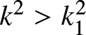 $k^2 \gt k_1^2$ and, thus,
  $\widehat{\Lambda}(k)$ can be diagonalized for such values. The associated change of basis is represented by a matrix
  $S(k)$, whose columns are comprised of eigenvectors of
  $\widehat{\Lambda}(k)$, and its inverse, which are given by
 \begin{align*} S(k) = \begin{pmatrix} \frac{1+k^2}{\mu(k)} & -\frac{1+k^2}{\mu(k)}\\ 1 & 1 \end{pmatrix}, \qquad S(k)^{-1} = \frac12\begin{pmatrix} \frac{\mu(k)}{4 k^2+4} & 1 \\
-\frac{\mu(k)}{4 k^2+4} & 1 \end{pmatrix}.
\end{align*}
\begin{align*} S(k) = \begin{pmatrix} \frac{1+k^2}{\mu(k)} & -\frac{1+k^2}{\mu(k)}\\ 1 & 1 \end{pmatrix}, \qquad S(k)^{-1} = \frac12\begin{pmatrix} \frac{\mu(k)}{4 k^2+4} & 1 \\
-\frac{\mu(k)}{4 k^2+4} & 1 \end{pmatrix}.
\end{align*} One readily observes that the coefficients of  $S(\cdot)$ and
  $S(\cdot)^{-1}$ are bounded on
 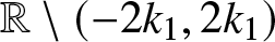 $\mathbb{R} \setminus (-2k_1,2k_1)$. Moreover, it holds
 \begin{align*}
\lambda_-(k) \leq -\dfrac{1}{2}\alpha k^2, \qquad \lambda_+(k) \leq -\dfrac{1}{\alpha}
\end{align*}
\begin{align*}
\lambda_-(k) \leq -\dfrac{1}{2}\alpha k^2, \qquad \lambda_+(k) \leq -\dfrac{1}{\alpha}
\end{align*}for 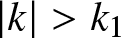 $|k| \gt k_1$. We conclude that there exists
  $\theta_2 \gt 0$ such that the matrix exponential and its temporal derivative
 \begin{align*}
\partial_t^j \mathrm{e}^{\widehat{\Lambda}(k) t} = S(k)^{-1} \mathrm{diag}\left(\lambda_+(k)^j \mathrm{e}^{\lambda_+(k) t}, \lambda_-(k)^j\mathrm{e}^{\lambda_-(k) t}\right) S(k),
\end{align*}
\begin{align*}
\partial_t^j \mathrm{e}^{\widehat{\Lambda}(k) t} = S(k)^{-1} \mathrm{diag}\left(\lambda_+(k)^j \mathrm{e}^{\lambda_+(k) t}, \lambda_-(k)^j\mathrm{e}^{\lambda_-(k) t}\right) S(k),
\end{align*}obey the estimate
 \begin{equation}
t^j \left|\partial_t^j \mathrm{e}^{\widehat{\Lambda}(k) t}\right| \lesssim \mathrm{e}^{-\theta_2 t},
\end{equation}
\begin{equation}
t^j \left|\partial_t^j \mathrm{e}^{\widehat{\Lambda}(k) t}\right| \lesssim \mathrm{e}^{-\theta_2 t},
\end{equation}for  $k \in \mathbb{R} \setminus (-2k_1,2k_1)$,
  $j = 0,1$ and
  $t \geq 0$. To bound the matrix exponential
  $\mathrm{e}^{\widehat{\Lambda}(k) t}$ and its temporal derivative on the compact set
  $\smash{J \overset{\scriptscriptstyle{\mathrm{def}}}{=} [-2k_1,-k_0/2] \cup [k_0/2,2k_1]}$, we collect some facts from [Reference Arendt, Grabosch, Greiner, Groh, Lotz, Moustakas, Nagel, Neubrander and Schlotterbeck1, Chapter A-III, §7]. Firstly, since
  $J$ is compact and
  $\widehat{\Lambda}$ is continuous on
  $J$, the multiplication operator
  $A \colon f \mapsto \widehat{\Lambda} f$ generates a strongly continuous semigroup
  $(T(t))_{t \geq 0}$ on
  $C(J,\mathbb{C}^2)$, which is given by
 \begin{equation*}(T(t)f)(k) = \mathrm{e}^{\widehat{\Lambda}(k) t} f(k), \qquad k \in J.\end{equation*}
 Secondly, the growth bound of the semigroup  $(T(t))_{t \geq 0}$ coincides with the spectral bound of
  $A$. Thirdly, the spectrum of
  $A$ is given by
 \begin{equation*}\sigma(A) = \bigcup_{k \in J} \sigma(\widehat{\Lambda}(k)).\end{equation*}
 Combining the latter three observations with (4.6) yields that the growth bound of the semigroup  $(T(t))_{t \geq 0}$ is smaller than
  $-\theta_1$, which implies
 \begin{align*}
\left|\mathrm{e}^{\widehat{\Lambda}(k) t}\right| \lesssim \mathrm{e}^{-\theta_1 t}, \qquad \left|\partial_t\mathrm{e}^{\widehat{\Lambda}(k) t}\right| = \left|\hat{\Lambda}(k) \mathrm{e}^{\widehat{\Lambda}(k) t}\right| \lesssim \mathrm{e}^{-\theta_1 t},
\end{align*}
\begin{align*}
\left|\mathrm{e}^{\widehat{\Lambda}(k) t}\right| \lesssim \mathrm{e}^{-\theta_1 t}, \qquad \left|\partial_t\mathrm{e}^{\widehat{\Lambda}(k) t}\right| = \left|\hat{\Lambda}(k) \mathrm{e}^{\widehat{\Lambda}(k) t}\right| \lesssim \mathrm{e}^{-\theta_1 t},
\end{align*}for all  $t \geq 0$ and
  $k \in J$. Combining the latter with (4.9) yields a constant
  $\theta_3 \gt 0$ such that
 \begin{equation}
t^j \left|\partial_t^j \mathrm{e}^{\widehat{\Lambda}(k) t}\right| \lesssim \mathrm{e}^{-\theta_3 t},
\end{equation}
\begin{equation}
t^j \left|\partial_t^j \mathrm{e}^{\widehat{\Lambda}(k) t}\right| \lesssim \mathrm{e}^{-\theta_3 t},
\end{equation}for  $j = 0,1$,
  $t \geq 0$ and
  $k \in \mathbb{R} \setminus [-\frac{k_0}{2},\frac{k_0}{2}]$, proving the first estimate in (4.7).
We proceed with the second estimate in (4.7). Firstly, we express the derivative as
 \begin{equation}
\partial_k \mathrm{e}^{\widehat{\Lambda}(k) t} = t\int_0^1 \mathrm{e}^{\widehat{\Lambda}(k) l t} \hat{\Lambda}'(k) \mathrm{e}^{\widehat{\Lambda}(k) (1-l) t} \mathrm{d} l.
\end{equation}
\begin{equation}
\partial_k \mathrm{e}^{\widehat{\Lambda}(k) t} = t\int_0^1 \mathrm{e}^{\widehat{\Lambda}(k) l t} \hat{\Lambda}'(k) \mathrm{e}^{\widehat{\Lambda}(k) (1-l) t} \mathrm{d} l.
\end{equation}Next, we apply the estimate (3.5) and obtain
 \begin{align*}
\left|\partial_k \mathrm{e}^{\widehat{\Lambda}(k) t} W\right| \leq t \int_0^1 \left|\mathrm{e}^{\widehat{\Lambda}(k) l t} \right| \left|\hat{\Lambda}(k) \mathrm{e}^{\widehat{\Lambda}(k) (1-l) t}W\right|^{\frac12} \left|\mathrm{e}^{\widehat{\Lambda}(k) (1-l) t}W\right|^{\frac12} \mathrm{d} l,
\end{align*}
\begin{align*}
\left|\partial_k \mathrm{e}^{\widehat{\Lambda}(k) t} W\right| \leq t \int_0^1 \left|\mathrm{e}^{\widehat{\Lambda}(k) l t} \right| \left|\hat{\Lambda}(k) \mathrm{e}^{\widehat{\Lambda}(k) (1-l) t}W\right|^{\frac12} \left|\mathrm{e}^{\widehat{\Lambda}(k) (1-l) t}W\right|^{\frac12} \mathrm{d} l,
\end{align*}for  $W \in \mathbb{C}^2$,
  $k \in \mathbb{R}$ and
  $t \geq 0$. So, using (4.10), we arrive at
 \begin{align*}
\left|\partial_k \mathrm{e}^{\widehat{\Lambda}(k) t} W\right| \lesssim t \mathrm{e}^{-\theta_0 t} \int_0^1 \frac{1}{\sqrt{(1-l)t}} \mathrm{d} l \left|W\right| \lesssim \sqrt{t}\, \mathrm{e}^{-\theta_3 t} \left|W\right| \lesssim \mathrm{e}^{-\frac{\theta_3}{2} t} \left|W\right|,
\end{align*}
\begin{align*}
\left|\partial_k \mathrm{e}^{\widehat{\Lambda}(k) t} W\right| \lesssim t \mathrm{e}^{-\theta_0 t} \int_0^1 \frac{1}{\sqrt{(1-l)t}} \mathrm{d} l \left|W\right| \lesssim \sqrt{t}\, \mathrm{e}^{-\theta_3 t} \left|W\right| \lesssim \mathrm{e}^{-\frac{\theta_3}{2} t} \left|W\right|,
\end{align*}for  $W \in \mathbb{C}^2$,
  $k \in \mathbb{R} \setminus [-\frac{k0}{2},\frac{k0}{2}]$ and
  $t \geq 0$, which proves the second estimate in (4.7).
Finally, we obtain bounds for  $k\in [-k_0, k_0]$. For such values, the matrix
  $\smash{\widehat{\Lambda}(k)}$ is diagonalizable and both
  $S(\cdot)$ and
  $S^{-1}(\cdot)$ are bounded on
  $[-k_0,k_0]$. Moreover, we have
  $|\hat{\Lambda}'(k)| \lesssim |k|$ for
  $k \in [-k_0,k_0]$. Combining the latter two observations with (4.5) and (4.11) readily yields the last estimate (4.8), which finishes the proof.
Remark 4.2. In addition to the viscous damping term  $-\alpha u_{txx}$, it is possible to include the first-order damping term
  $\gamma u_t$ with
  $\gamma \gt 0$ on the left-hand side of (1.2), cf. [Reference Aviles and Sandefur2, Reference Potier-Ferry34]. This dissipative term models internal resistance or frictional forces in the viscoelastic material. In contrast to the viscous damping term
  $-\alpha u_{txx}$, it dampens the amplitude of solutions without smoothing out oscillations. In the presence of the first-order damping term
  $\gamma u_t$, the spectrum of the linearization is given by
 \begin{equation}
\left\{-\dfrac{1}{2}\left(\gamma + \alpha k^2\right) \pm \sqrt{\dfrac{1}{4}\left(\gamma + \alpha k^2\right)^2 - 1 - k^2} : k \in \mathbb{R}\right\}\!,
\end{equation}
\begin{equation}
\left\{-\dfrac{1}{2}\left(\gamma + \alpha k^2\right) \pm \sqrt{\dfrac{1}{4}\left(\gamma + \alpha k^2\right)^2 - 1 - k^2} : k \in \mathbb{R}\right\}\!,
\end{equation}see Figure 3. In contrast to our situation, the spectrum is confined to the open left-half plane for  $\gamma \gt 0$ and it follows from standard arguments, cf. [Reference Cazenave and Haraux7, Section 10], that the equilibrium state
  $u(x,t) = 0$ in (1.2) is exponentially stable for
  $\gamma \gt 0$. That is, solutions with small initial data decay at an exponential rate.
5. Mode filters

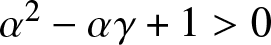
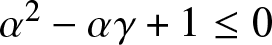

We are ready to start the reduction process that is necessary to close the nonlinear argument. Let  $\mathcal{X}$ denote the space
  $X_0$ or
  $Y_0$. Take
  $u_0,w_0 \in \mathcal{X}$ satisfying (1.8) (in case
  $\mathcal{X} = X_0$) or satisfying (1.17) (in case
  $\mathcal{X} = Y_0$). Clearly, there exists a constant
  $K \gt 0$, independent of
  $u_0$ and
  $w_0$, such that
 \begin{align*} U_0 \overset{\scriptscriptstyle{\mathrm{def}}}{=} \begin{pmatrix}u_0 \\ (1-\partial_x^2)^{-1}\left(w_0 - \frac{\alpha}{2} \partial_x^2 u_0\right)\end{pmatrix} \in \mathcal{X},\end{align*}
obeys
 \begin{equation}
\|U_0\|_{\mathcal{X}} \leq KE_0.
\end{equation}
\begin{equation}
\|U_0\|_{\mathcal{X}} \leq KE_0.
\end{equation} Moreover, Proposition 3.2 yields a time  $T_{\max} \in (0,\infty]$ and a unique, maximally defined, mild solution
 \begin{equation}
U \in C\big([0,T_{\max}),\mathcal{X}\big),
\end{equation}
\begin{equation}
U \in C\big([0,T_{\max}),\mathcal{X}\big),
\end{equation}of (3.2) with initial condition  $U(0) = U_0$ such that, if
  $T_{\max} \lt \infty$, then (3.3) holds.
In the Fourier space system (3.2) reads
 \begin{equation}
\partial_t \widehat{U} = \widehat{\Lambda} \widehat{U} + \mathcal{F} \mathcal{N}\big(\mathcal{F}^{-1} \widehat{U}\big),
\end{equation}
\begin{equation}
\partial_t \widehat{U} = \widehat{\Lambda} \widehat{U} + \mathcal{F} \mathcal{N}\big(\mathcal{F}^{-1} \widehat{U}\big),
\end{equation}where  $\widehat{\Lambda}$ is the Fourier symbol of
  $\Lambda$ defined in (4.1).
To separate diffusive low-frequency modes from exponentially damped high-frequency modes and diagonalize the system at criticality, we introduce mode filters. Thus, let  $k_0 \gt 0$ be as in §4 and let
  $\chi \colon \mathbb{R} \to [0,1]$ be a smooth even cut-off function, whose support is contained in
  $(-k_0,k_0)$, such that
  $\chi(k) = 1$ for
  $k \in [-k_0/2,k_0/2]$. We decompose the solution
 \begin{equation}
\widehat{U}(t) = \chi \widehat{U}(t) + (1-\chi)\widehat{U}(t) \overset{\scriptscriptstyle{\mathrm{def}}}{=} \widehat{U}_\mathrm{c}(t) + \widehat{U}_\mathrm{s}(t), \qquad t \in [0,T_{\max})
\end{equation}
\begin{equation}
\widehat{U}(t) = \chi \widehat{U}(t) + (1-\chi)\widehat{U}(t) \overset{\scriptscriptstyle{\mathrm{def}}}{=} \widehat{U}_\mathrm{c}(t) + \widehat{U}_\mathrm{s}(t), \qquad t \in [0,T_{\max})
\end{equation}of (3.2) into a low- and high-frequency part. We note that, since  $U(t)$ is real-valued and
  $\chi$ is even, it holds
 \begin{equation}
\smash{\overline{\widehat{U}_\mathrm{c}(k,t)}} = \widehat{U}_\mathrm{c}(-k,t)
\end{equation}
\begin{equation}
\smash{\overline{\widehat{U}_\mathrm{c}(k,t)}} = \widehat{U}_\mathrm{c}(-k,t)
\end{equation}for each  $k \in \mathbb{R}$ and
  $t \in [0,T_{\max})$. Moreover, by (5.2), the smoothness of
  $\chi$ and the fact that
  $\chi$ is compactly supported, we obtain
 \begin{equation}
\widehat{U}, \widehat{U}_\mathrm{c}, |\cdot| \widehat{U}_\mathrm{c}, \widehat{U}_\mathrm{s} \in C\big([0,T_{\max}),W^{1,1}(\mathbb{R}) \cap W^{1,\infty}(\mathbb{R})\big),
\end{equation}
\begin{equation}
\widehat{U}, \widehat{U}_\mathrm{c}, |\cdot| \widehat{U}_\mathrm{c}, \widehat{U}_\mathrm{s} \in C\big([0,T_{\max}),W^{1,1}(\mathbb{R}) \cap W^{1,\infty}(\mathbb{R})\big),
\end{equation}in case  $\mathcal{X} = X_0$, and
 \begin{equation}
\widehat{U}, \widehat{U}_\mathrm{c}, \widehat{U}_\mathrm{s} \in C\big([0,T_{\max}),L^1(\mathbb{R}) \cap L^\infty(\mathbb{R})\big),
\end{equation}
\begin{equation}
\widehat{U}, \widehat{U}_\mathrm{c}, \widehat{U}_\mathrm{s} \in C\big([0,T_{\max}),L^1(\mathbb{R}) \cap L^\infty(\mathbb{R})\big),
\end{equation}in case  $\mathcal{X} = Y_0$.
Multiplying (5.3) with  $\chi$ and
  $1-\chi$, we arrive at the system
 \begin{equation}
\partial_t \widehat{U}_\mathrm{c} = \widehat{\Lambda} \widehat{U}_\mathrm{c} + \chi \mathcal{F} \mathcal{N}\left(\mathcal{F}^{-1}\big(\widehat{U}_\mathrm{c} + \widehat{U}_\mathrm{s}\big)\right),
\end{equation}
\begin{equation}
\partial_t \widehat{U}_\mathrm{c} = \widehat{\Lambda} \widehat{U}_\mathrm{c} + \chi \mathcal{F} \mathcal{N}\left(\mathcal{F}^{-1}\big(\widehat{U}_\mathrm{c} + \widehat{U}_\mathrm{s}\big)\right),
\end{equation} \begin{equation}
\partial_t \widehat{U}_\mathrm{s} = \widehat{\Lambda} \widehat{U}_\mathrm{s} + (1-\chi) \mathcal{F} \mathcal{N}\left(\mathcal{F}^{-1}\big(\widehat{U}_\mathrm{c} + \widehat{U}_\mathrm{s}\big)\right),
\end{equation}
\begin{equation}
\partial_t \widehat{U}_\mathrm{s} = \widehat{\Lambda} \widehat{U}_\mathrm{s} + (1-\chi) \mathcal{F} \mathcal{N}\left(\mathcal{F}^{-1}\big(\widehat{U}_\mathrm{c} + \widehat{U}_\mathrm{s}\big)\right),
\end{equation} for the new variables  $\widehat{U}_\mathrm{c}$ and
  $\widehat{U}_\mathrm{s}$.
The Duhamel formulation associated with (5.8)–(5.9) reads
 \begin{equation}
\widehat{U}_\mathrm{c}(k,t) = \mathrm{e}^{\widehat{\Lambda}(k) t} \chi(k) \widehat{U}(k,0) + \int_0^t \mathrm{e}^{\widehat{\Lambda}(k)(t-s)} \chi(k) \mathcal{F} \mathcal{N}\left(\mathcal{F}^{-1}\big(\widehat{U}_\mathrm{c}(s) + \widehat{U}_\mathrm{s}(s)\big)\right)\!(k) \, \mathrm{d} s,
\end{equation}
\begin{equation}
\widehat{U}_\mathrm{c}(k,t) = \mathrm{e}^{\widehat{\Lambda}(k) t} \chi(k) \widehat{U}(k,0) + \int_0^t \mathrm{e}^{\widehat{\Lambda}(k)(t-s)} \chi(k) \mathcal{F} \mathcal{N}\left(\mathcal{F}^{-1}\big(\widehat{U}_\mathrm{c}(s) + \widehat{U}_\mathrm{s}(s)\big)\right)\!(k) \, \mathrm{d} s,
\end{equation} \begin{equation}
\begin{aligned}
\widehat{U}_\mathrm{s}(k,t) &= \mathrm{e}^{\widehat{\Lambda}(k) t} (1-\chi(k)) \widehat{U}(k,0)\\
& \qquad + \, \int_0^t \mathrm{e}^{\widehat{\Lambda}(k)(t-s)} (1-\chi(k)) \mathcal{F} \mathcal{N}\left(\mathcal{F}^{-1}\big(\widehat{U}_\mathrm{c}(s) + \widehat{U}_\mathrm{s}(s)\big)\right)\!(k) \, \mathrm{d} s,
\end{aligned}
\end{equation}
\begin{equation}
\begin{aligned}
\widehat{U}_\mathrm{s}(k,t) &= \mathrm{e}^{\widehat{\Lambda}(k) t} (1-\chi(k)) \widehat{U}(k,0)\\
& \qquad + \, \int_0^t \mathrm{e}^{\widehat{\Lambda}(k)(t-s)} (1-\chi(k)) \mathcal{F} \mathcal{N}\left(\mathcal{F}^{-1}\big(\widehat{U}_\mathrm{c}(s) + \widehat{U}_\mathrm{s}(s)\big)\right)\!(k) \, \mathrm{d} s,
\end{aligned}
\end{equation} with  $k \in \mathbb{R}$ and
  $t \in [0,T_{\max})$.
6. Separating relevant from irrelevant nonlinear terms
As outlined before, our goal is to close a nonlinear argument through iterative estimates on the Duhamel formulation (5.10)–(5.11). In this section, we isolate those nonlinear terms in (5.10)–(5.11), which cannot be controlled through standard iterative  $L^1$-
 $L^\infty$-estimates, and establish estimates on the irrelevant residual terms.
Lemma 4.1 implies that 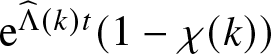 $\smash{\mathrm{e}^{\widehat{\Lambda}(k) t} (1-\chi(k))}$ is exponentially decaying over time, whereas
 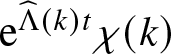 $\smash{\mathrm{e}^{\widehat{\Lambda}(k) t} \chi(k)}$ only decays diffusively. Therefore, one expects that the decay of
  $\widehat{U}_\mathrm{s}(t)$ is dictated by the slowest decaying nonlinear terms in
  $\widehat{U}_\mathrm{c}$, which are the quadratic terms. Hence,
  $\widehat{U}_\mathrm{s}(t)$ is expected to decay at a higher rate than
  $\widehat{U}_\mathrm{c}(t)$. Thanks to the higher decay rate of
  $\widehat{U}_\mathrm{s}(t)$ in combination with the fact that it vanishes at the critical frequency
  $k = 0$, any nonlinear term in (5.10) with a
  $\widehat{U}_\mathrm{s}$-contribution can be controlled, as can any quartic or higher-order nonlinear term in (5.10) as outlined in §1.2. All in all, the only nonlinear terms that cannot be controlled through standard iterative
  $L^1$-
 $L^\infty$-estimates are the quadratic and cubic terms in (5.10)–(5.11).
We split off these terms by expanding  $N \in C^4(\mathbb{R})$ as a Taylor series
 \begin{equation}
N(u) = 2\pi\kappa u^2 + 4\pi^2\beta u^3 + R(u)
\end{equation}
\begin{equation}
N(u) = 2\pi\kappa u^2 + 4\pi^2\beta u^3 + R(u)
\end{equation}with coefficients  $\beta,\kappa \in \mathbb{R}$, where there exists a constant
  $C \gt 0$ such that the quartic remainder
  $R\colon \mathbb{R} \to \mathbb{R}$ obeys the estimate
 \begin{align*}
|R(u)| \leq C|u|^4,
\end{align*}
\begin{align*}
|R(u)| \leq C|u|^4,
\end{align*}for  $u \in [-1,1]$. The critical quadratic term in (5.10) is then given by
 \begin{equation}
\int_0^t \chi(k) \mathrm{e}^{\widehat{\Lambda}(k) (t-s)} B_2\big(\widehat{U}_\mathrm{c}(s),\widehat{U}_\mathrm{c}(s)\big)(k) \mathrm{d} l \mathrm{d} s,
\end{equation}
\begin{equation}
\int_0^t \chi(k) \mathrm{e}^{\widehat{\Lambda}(k) (t-s)} B_2\big(\widehat{U}_\mathrm{c}(s),\widehat{U}_\mathrm{c}(s)\big)(k) \mathrm{d} l \mathrm{d} s,
\end{equation}where  $B_2$ is the symmetric bilinear form on
  $
\mathcal{X}$ given by
$
\mathcal{X}$ given by
 \begin{align*}
B_2({\widehat{V}}, \widehat{W})(k) = \int_\mathbb{R} N_2(k,l)\big({\widehat{V}},{\widehat{W}}) \mathrm{d} l, \qquad N_2(k,l)\big({\widehat{V}},{\widehat{W}}\big) \overset{\scriptscriptstyle{\mathrm{def}}}{=} \frac{\kappa}{1+k^2} {\widehat{V}}_1(k-l) \widehat{W}_1(l) \mathbf{e}_2,
\end{align*}
\begin{align*}
B_2({\widehat{V}}, \widehat{W})(k) = \int_\mathbb{R} N_2(k,l)\big({\widehat{V}},{\widehat{W}}) \mathrm{d} l, \qquad N_2(k,l)\big({\widehat{V}},{\widehat{W}}\big) \overset{\scriptscriptstyle{\mathrm{def}}}{=} \frac{\kappa}{1+k^2} {\widehat{V}}_1(k-l) \widehat{W}_1(l) \mathbf{e}_2,
\end{align*}Moreover, the critical cubic term in (5.10) reads
 \begin{equation}
\int_0^t \chi(k) \mathrm{e}^{\widehat{\Lambda}(k) (t-s)} B_3\big(\widehat{U}_\mathrm{c}(s),\widehat{U}_\mathrm{c}(s),\widehat{U}_\mathrm{c}(s)\big)(k) \mathrm{d} s,
\end{equation}
\begin{equation}
\int_0^t \chi(k) \mathrm{e}^{\widehat{\Lambda}(k) (t-s)} B_3\big(\widehat{U}_\mathrm{c}(s),\widehat{U}_\mathrm{c}(s),\widehat{U}_\mathrm{c}(s)\big)(k) \mathrm{d} s,
\end{equation}where  $B_3$ is the symmetric trilinear form on
  $\mathcal{X}$ given by
 \begin{align*}
B_3({\widehat{V}}, \widehat{W}, \widehat{Z})(k) &= \int_\mathbb{R} \int_\mathbb{R} N_3(k,l_1,l_2)\big({\widehat{V}},{\widehat{W}},\widehat{Z}\big) \mathrm{d} l_1 \mathrm{d} l_2, \\
N_3(k,l_1,l_2)\big({\widehat{V}},{\widehat{W}},\widehat{Z}\big) &\overset{\scriptscriptstyle{\mathrm{def}}}{=} \frac{\beta}{1+k^2} {\widehat{V}}_1(k-l_1) \widehat{W}_1(l_1-l_2) \widehat{Z}_1(l_2) \mathbf{e}_2.
\end{align*}
\begin{align*}
B_3({\widehat{V}}, \widehat{W}, \widehat{Z})(k) &= \int_\mathbb{R} \int_\mathbb{R} N_3(k,l_1,l_2)\big({\widehat{V}},{\widehat{W}},\widehat{Z}\big) \mathrm{d} l_1 \mathrm{d} l_2, \\
N_3(k,l_1,l_2)\big({\widehat{V}},{\widehat{W}},\widehat{Z}\big) &\overset{\scriptscriptstyle{\mathrm{def}}}{=} \frac{\beta}{1+k^2} {\widehat{V}}_1(k-l_1) \widehat{W}_1(l_1-l_2) \widehat{Z}_1(l_2) \mathbf{e}_2.
\end{align*}Finally, the nonlinear remainder in (5.10) is
 \begin{align*}
\int_0^t \mathrm{e}^{\widehat{\Lambda}(k)(t-s)} \chi(k) \mathcal{E}\big(\widehat{U}_\mathrm{c}(s),\widehat{U}_\mathrm{s}(s)\big)(k) \mathrm{d} s,
\end{align*}
\begin{align*}
\int_0^t \mathrm{e}^{\widehat{\Lambda}(k)(t-s)} \chi(k) \mathcal{E}\big(\widehat{U}_\mathrm{c}(s),\widehat{U}_\mathrm{s}(s)\big)(k) \mathrm{d} s,
\end{align*}where  $\mathcal{E} \colon \mathcal{X} \times \mathcal{X} \to \mathcal{X}$ is the nonlinear operator given by
 \begin{align*}
\mathcal{E}\big({\widehat{V}},{\widehat{W}}\big) &= \mathcal{F} \mathcal{R}\left(\mathcal{F}^{-1}\big({\widehat{V}} + {\widehat{W}}\big)\right) + 2B_2\big({\widehat{V}},{\widehat{W}}\big) + B_2\big({\widehat{W}},{\widehat{W}}\big)\\
&\qquad \, + 3B_3\big({\widehat{V}},{\widehat{V}},{\widehat{W}})\big) + 3B_3\big({\widehat{V}},{\widehat{W}},{\widehat{W}}\big) + B_3\big({\widehat{W}},{\widehat{W}},{\widehat{W}}\big),
\end{align*}
\begin{align*}
\mathcal{E}\big({\widehat{V}},{\widehat{W}}\big) &= \mathcal{F} \mathcal{R}\left(\mathcal{F}^{-1}\big({\widehat{V}} + {\widehat{W}}\big)\right) + 2B_2\big({\widehat{V}},{\widehat{W}}\big) + B_2\big({\widehat{W}},{\widehat{W}}\big)\\
&\qquad \, + 3B_3\big({\widehat{V}},{\widehat{V}},{\widehat{W}})\big) + 3B_3\big({\widehat{V}},{\widehat{W}},{\widehat{W}}\big) + B_3\big({\widehat{W}},{\widehat{W}},{\widehat{W}}\big),
\end{align*}with
 \begin{align*}
\mathcal{R}(V) = \left(1-\partial_x^2\right)^{-1} R(V_1) \mathbf{e}_2.
\end{align*}
\begin{align*}
\mathcal{R}(V) = \left(1-\partial_x^2\right)^{-1} R(V_1) \mathbf{e}_2.
\end{align*}The next result establishes estimates on the noncritical nonlinear terms in (5.10)–(5.11).
Lemma 6.1. We have
 \begin{align*}
\left\|\partial_k^j \mathcal{F} \mathcal{N}\left(\mathcal{F}^{-1}\big({\widehat{V}}\big)\right)\right\|_{L^p} &\lesssim \big\|{\widehat{V}}\big\|_{W^{j,1}} \big\|{\widehat{V}}\big\|_{L^p},
\end{align*}
\begin{align*}
\left\|\partial_k^j \mathcal{F} \mathcal{N}\left(\mathcal{F}^{-1}\big({\widehat{V}}\big)\right)\right\|_{L^p} &\lesssim \big\|{\widehat{V}}\big\|_{W^{j,1}} \big\|{\widehat{V}}\big\|_{L^p},
\end{align*}for  $j = 0,1$,
  $p = 1,\infty$ and
  ${\widehat{V}} \in L^\infty(\mathbb{R}) \cap W^{j,1}(\mathbb{R})$ satisfying
  $\|{\widehat{V}}\|_{L^1} \leq 1$. Moreover, it holds
 \begin{align*}
\left|\partial_k^j \mathcal{E}\big({\widehat{V}},(1-\chi){\widehat{W}}\big)(k)\right| &\lesssim \big\|{\widehat{V}}\big\|_{L^1}^2 \big\|{\widehat{V}}\big\|_{W^{j,1}} + \big\|(1-\chi){\widehat{W}}\big\|_{W^{j,1}}\big\|(1-\chi){\widehat{W}}\big\|_{L^\infty} \\
&\qquad + \, |k| \big\|(1-\chi){\widehat{W}}\big\|_{L^\infty} \big\|{\widehat{V}}\big\|_{W^{j,1}} + \big\|(1-\chi){\widehat{W}}\big\|_{L^\infty} \big\||\cdot|{\widehat{V}}\big\|_{W^{j,1}}\\
&\qquad + \, \big\|(1-\chi){\widehat{W}}\big\|_{L^1} \big\|{\widehat{V}}\big\|_{W^{j,1}},
\end{align*}
\begin{align*}
\left|\partial_k^j \mathcal{E}\big({\widehat{V}},(1-\chi){\widehat{W}}\big)(k)\right| &\lesssim \big\|{\widehat{V}}\big\|_{L^1}^2 \big\|{\widehat{V}}\big\|_{W^{j,1}} + \big\|(1-\chi){\widehat{W}}\big\|_{W^{j,1}}\big\|(1-\chi){\widehat{W}}\big\|_{L^\infty} \\
&\qquad + \, |k| \big\|(1-\chi){\widehat{W}}\big\|_{L^\infty} \big\|{\widehat{V}}\big\|_{W^{j,1}} + \big\|(1-\chi){\widehat{W}}\big\|_{L^\infty} \big\||\cdot|{\widehat{V}}\big\|_{W^{j,1}}\\
&\qquad + \, \big\|(1-\chi){\widehat{W}}\big\|_{L^1} \big\|{\widehat{V}}\big\|_{W^{j,1}},
\end{align*}for  $j = 0,1$,
  $k \in \mathbb{R}$ and
  ${\widehat{V}},{\widehat{W}} \in W^{j,1}(\mathbb{R}) \cap L^\infty(\mathbb{R})$ satisfying
  $\|{\widehat{V}}\|_{L^1 \cap L^\infty}, \|{\widehat{W}}\|_{L^1 \cap L^\infty} \leq 1$ and
  $\||\cdot| {\widehat{V}}\|_{W^{j,1}} \lt \infty$.
Proof. Recall that  $1-\chi$ vanishes on
  $[-k_0/2,k_0/2]$. So, letting
  $\upsilon \colon \mathbb{R} \to [0,1]$ be a smooth function supported on
  $[-k_0/2,k_0/2]$ with
  $\upsilon(0) = 1$, we obtain
 \begin{align*}
B_2\big({\widehat{V}},(1-\chi){\widehat{W}}\big)(k) = \int_\mathbb{R} \frac{1-\upsilon(l)}{l} (k + (l-k)) N_2(k,l)\big({\widehat{V}},(1-\chi){\widehat{W}}\big) \mathrm{d} l,
\end{align*}
\begin{align*}
B_2\big({\widehat{V}},(1-\chi){\widehat{W}}\big)(k) = \int_\mathbb{R} \frac{1-\upsilon(l)}{l} (k + (l-k)) N_2(k,l)\big({\widehat{V}},(1-\chi){\widehat{W}}\big) \mathrm{d} l,
\end{align*}for  $k \in \mathbb{R}$. Upon noticing that
  $l \mapsto \frac{1-\upsilon(l)}{l}$ is bounded on
  $\mathbb{R}$, we deduce
 \begin{equation}
\left|\partial_k^j B_2\big({\widehat{V}},(1-\chi){\widehat{W}}\big)(k)\right| \lesssim |k| \big\|{\widehat{V}}\big\|_{W^{j,1}} \big\|{\widehat{W}}\big\|_{L^\infty} + \big\||\cdot| {\widehat{V}}\big\|_{W^{j,1}} \big\|{\widehat{W}}\big\|_{L^\infty},
\end{equation}
\begin{equation}
\left|\partial_k^j B_2\big({\widehat{V}},(1-\chi){\widehat{W}}\big)(k)\right| \lesssim |k| \big\|{\widehat{V}}\big\|_{W^{j,1}} \big\|{\widehat{W}}\big\|_{L^\infty} + \big\||\cdot| {\widehat{V}}\big\|_{W^{j,1}} \big\|{\widehat{W}}\big\|_{L^\infty},
\end{equation}for  $j = 0,1$,
  $k \in \mathbb{R}$,
  ${\widehat{V}} \in W^{j,1}(\mathbb{R})$ and
  ${\widehat{W}} \in L^\infty(\mathbb{R})$ with
  $\||\cdot|{\widehat{V}}\|_{W^{j,1}} \lt \infty$. On the other hand, using Young’s convolution inequality, we infer
 \begin{equation}
\begin{aligned}
\left\|\partial_k^j B_2\big({\widehat{V}},{\widehat{W}}\big) \right\|_{L^\infty} &\lesssim \big\|{\widehat{V}}\big\|_{W^{j,1}} \big\|{\widehat{W}}\big\|_{L^\infty},\\
\left\|\partial_k^j B_2\big({\widehat{V}},\widehat{Z}\big) \right\|_{L^1} &\lesssim \big\|{\widehat{V}}\big\|_{W^{j,1}} \big\|\widehat{Z}\big\|_{L^1},\\
\left\|\partial_k^j B_3\big({\widehat{V}},{\widehat{W}},\widehat{Z}\big)\right\|_{L^\infty} &\lesssim \big\|{\widehat{V}}\big\|_{W^{j,1}} \big\|{\widehat{W}}\big\|_{L^\infty} \big\|\widehat{Z}\big\|_{L^1},
\end{aligned}
\end{equation}
\begin{equation}
\begin{aligned}
\left\|\partial_k^j B_2\big({\widehat{V}},{\widehat{W}}\big) \right\|_{L^\infty} &\lesssim \big\|{\widehat{V}}\big\|_{W^{j,1}} \big\|{\widehat{W}}\big\|_{L^\infty},\\
\left\|\partial_k^j B_2\big({\widehat{V}},\widehat{Z}\big) \right\|_{L^1} &\lesssim \big\|{\widehat{V}}\big\|_{W^{j,1}} \big\|\widehat{Z}\big\|_{L^1},\\
\left\|\partial_k^j B_3\big({\widehat{V}},{\widehat{W}},\widehat{Z}\big)\right\|_{L^\infty} &\lesssim \big\|{\widehat{V}}\big\|_{W^{j,1}} \big\|{\widehat{W}}\big\|_{L^\infty} \big\|\widehat{Z}\big\|_{L^1},
\end{aligned}
\end{equation}for  $j = 0,1$,
  ${\widehat{V}} \in W^{j,1}(\mathbb{R})$,
  ${\widehat{W}} \in L^\infty(\mathbb{R})$ and
  $\widehat{Z} \in L^1(\mathbb{R})$.
Next, we expand
 \begin{equation}
\mathcal{F} \mathcal{N}\big(\mathcal{F}^{-1}{\widehat{V}}\big)\big) = B_2\big({\widehat{V}},{\widehat{V}}\big) + \mathcal{F} \mathcal{R}_2\left(\mathcal{F}^{-1}\big({\widehat{V}}\big)\right),
\end{equation}
\begin{equation}
\mathcal{F} \mathcal{N}\big(\mathcal{F}^{-1}{\widehat{V}}\big)\big) = B_2\big({\widehat{V}},{\widehat{V}}\big) + \mathcal{F} \mathcal{R}_2\left(\mathcal{F}^{-1}\big({\widehat{V}}\big)\right),
\end{equation}with  $\mathcal{R}_2(V)$ defined by
 \begin{equation}
\mathcal{R}_2(V) = (1-\partial_x^2)^{-1} R_0(V_1)\mathbf{e}_2, \qquad R_0(z) \overset{\scriptscriptstyle{\mathrm{def}}}{=} N(z) - 2\pi \kappa z^2.
\end{equation}
\begin{equation}
\mathcal{R}_2(V) = (1-\partial_x^2)^{-1} R_0(V_1)\mathbf{e}_2, \qquad R_0(z) \overset{\scriptscriptstyle{\mathrm{def}}}{=} N(z) - 2\pi \kappa z^2.
\end{equation} The expansion (6.1) yields  $|R_0(z)| \lesssim |z|^3$ and
  $|R(z)| \lesssim |z|^4$ for
  $z \in [-1,1]$. So, using the facts that we have
  $\|V\|_{L^2}^2 \leq \|V\|_{L^1} \|V\|_{L^\infty}$ for
  $V \in L^1(\mathbb{R}) \cap L^\infty(\mathbb{R})$ and the Fourier transform is an isomorphism on
  $L^2(\mathbb{R})$ and it maps
  $L^1(\mathbb{R})$ continuously into
  $L^\infty(\mathbb{R})$, we establish
 \begin{equation}
\begin{aligned}
\left\|\partial_k^j \mathcal{F} \mathcal{R}_2\left(\mathcal{F}^{-1}\big({\widehat{V}}\big)\right)\right\|_{L^\infty} &\lesssim \left\|\frac{1}{1+|\cdot|^{2}}\right\|_{W^{j,\infty}} \left\|(1+|\cdot|^j) R_0\left(\mathcal{F}^{-1}\big({\widehat{V}}\big)_1\right)\right\|_{L^1}\\
&\lesssim \left\|\mathcal{F}^{-1}\big({\widehat{V}}\big)\right\|_{L^2}^2 \left\|(1+|\cdot|^j)\mathcal{F}^{-1}\big({\widehat{V}}\big)\right\|_{L^\infty}\\
&\lesssim \big\|{\widehat{V}}\big\|_{L^2}^2 \big\|{\widehat{V}}\big\|_{W^{j,1}} \lesssim \big\|{\widehat{V}}\big\|_{L^1} \big\|{\widehat{V}}\big\|_{W^{j,1}},\\
\left\|\partial_k^j \mathcal{F} \mathcal{R}_2\left(\mathcal{F}^{-1}\big({\widehat{V}}\big)\right)\right\|_{L^1} &\lesssim \left\|\frac{1}{1+|\cdot|^{2}}\right\|_{H^j} \left\| (1+|\cdot|^j) R_0\left(\mathcal{F}^{-1}\big({\widehat{V}}\big)_1\right)\right\|_{L^2}\\
&\lesssim \big\|\mathcal{F}^{-1}\big({\widehat{V}}\big)\big\|_{L^2} \big\|\mathcal{F}^{-1}\big({\widehat{V}}\big)\big\|_{L^\infty} \big\|(1+|\cdot|^j) \mathcal{F}^{-1}\big({\widehat{V}}\big)\big\|_{L^\infty}\\
&\lesssim \big\|{\widehat{V}}\big\|_{L^2} \big\|{\widehat{V}}\big\|_{L^1} \big\|{\widehat{V}}\big\|_{W^{j,1}}\lesssim \big\|{\widehat{V}}\big\|_{L^1} \big\|{\widehat{V}}\big\|_{W^{j,1}},
\end{aligned}
\end{equation}
\begin{equation}
\begin{aligned}
\left\|\partial_k^j \mathcal{F} \mathcal{R}_2\left(\mathcal{F}^{-1}\big({\widehat{V}}\big)\right)\right\|_{L^\infty} &\lesssim \left\|\frac{1}{1+|\cdot|^{2}}\right\|_{W^{j,\infty}} \left\|(1+|\cdot|^j) R_0\left(\mathcal{F}^{-1}\big({\widehat{V}}\big)_1\right)\right\|_{L^1}\\
&\lesssim \left\|\mathcal{F}^{-1}\big({\widehat{V}}\big)\right\|_{L^2}^2 \left\|(1+|\cdot|^j)\mathcal{F}^{-1}\big({\widehat{V}}\big)\right\|_{L^\infty}\\
&\lesssim \big\|{\widehat{V}}\big\|_{L^2}^2 \big\|{\widehat{V}}\big\|_{W^{j,1}} \lesssim \big\|{\widehat{V}}\big\|_{L^1} \big\|{\widehat{V}}\big\|_{W^{j,1}},\\
\left\|\partial_k^j \mathcal{F} \mathcal{R}_2\left(\mathcal{F}^{-1}\big({\widehat{V}}\big)\right)\right\|_{L^1} &\lesssim \left\|\frac{1}{1+|\cdot|^{2}}\right\|_{H^j} \left\| (1+|\cdot|^j) R_0\left(\mathcal{F}^{-1}\big({\widehat{V}}\big)_1\right)\right\|_{L^2}\\
&\lesssim \big\|\mathcal{F}^{-1}\big({\widehat{V}}\big)\big\|_{L^2} \big\|\mathcal{F}^{-1}\big({\widehat{V}}\big)\big\|_{L^\infty} \big\|(1+|\cdot|^j) \mathcal{F}^{-1}\big({\widehat{V}}\big)\big\|_{L^\infty}\\
&\lesssim \big\|{\widehat{V}}\big\|_{L^2} \big\|{\widehat{V}}\big\|_{L^1} \big\|{\widehat{V}}\big\|_{W^{j,1}}\lesssim \big\|{\widehat{V}}\big\|_{L^1} \big\|{\widehat{V}}\big\|_{W^{j,1}},
\end{aligned}
\end{equation}for  $j = 0,1$ and
  ${\widehat{V}} \in W^{j,1}(\mathbb{R}) \cap L^\infty(\mathbb{R})$ with
  $\|{\widehat{V}}\|_{L^1 \cap L^\infty} \leq 1$. Similarly, we obtain
 \begin{equation}
\begin{aligned}
\left\|\partial_k^j \mathcal{F} \mathcal{R}\left(\mathcal{F}^{-1}\big({\widehat{V}}\big)\right)\right\|_{L^\infty} &\lesssim \big\|{\widehat{V}}\big\|_{L^2}^2 \big\|{\widehat{V}}\big\|_{W^{j,1}} \big\|V\big\|_{L^1} \lesssim \big\|{\widehat{V}}\big\|_{L^1}^2 \big\|{\widehat{V}}\big\|_{W^{j,1}},
\end{aligned}
\end{equation}
\begin{equation}
\begin{aligned}
\left\|\partial_k^j \mathcal{F} \mathcal{R}\left(\mathcal{F}^{-1}\big({\widehat{V}}\big)\right)\right\|_{L^\infty} &\lesssim \big\|{\widehat{V}}\big\|_{L^2}^2 \big\|{\widehat{V}}\big\|_{W^{j,1}} \big\|V\big\|_{L^1} \lesssim \big\|{\widehat{V}}\big\|_{L^1}^2 \big\|{\widehat{V}}\big\|_{W^{j,1}},
\end{aligned}
\end{equation}for  $j = 0,1$ and
  ${\widehat{V}} \in W^{j,1}(\mathbb{R}) \cap L^\infty(\mathbb{R})$ with
  $\|{\widehat{V}}\|_{L^1 \cap L^\infty} \leq 1$. In summary, the desired bound on
  $\mathcal{F}\mathcal{N}(\mathcal{F}^{-1}({\widehat{V}}))$ follows by recalling (6.6) and combining the estimates (6.5) and (6.8), whereas the estimate on
  $\mathcal{E}({\widehat{V}},(1-\chi){\widehat{W}})$ follows by (6.4), (6.5) and (6.9).
7. Eliminating quadratic terms
The linear behaviour of (5.10) at the critical frequency  $k = 0$ is time-oscillatory. That is, the matrix
  $\smash{\mathrm{e}^{\widehat{\Lambda}(k)t}}$ has the eigenvalues
  $\mathrm{e}^{\pm \mathrm{i} t}$ at
  $k = 0$. We can leverage the oscillatory character of the integrals in (5.10) by integrating by parts with respect to time to eliminate potentially dangerous quadratic or cubic nonlinear terms, as long as the associated phase functions are nonzero, i.e., as long as we avoid time resonances. In this section, we show that quadratic terms are not time-resonant and can therefore be eliminated.
We will establish that the phase functions  $\phi_j^2 \colon \mathbb{R}^2 \to \mathbb{R}$ associated with the quadratic nonlinear term (6.2) in (5.10) are given by
 \begin{align*}
\phi^2_{j}(k,l) = \lambda_{j_0}(k) - \lambda_{j_1}(k - l) - \lambda_{j_2}(l),
\end{align*}
\begin{align*}
\phi^2_{j}(k,l) = \lambda_{j_0}(k) - \lambda_{j_1}(k - l) - \lambda_{j_2}(l),
\end{align*}with  $j = (j_0,j_1,j_2) \in \left\lbrace -1, 1 \right\rbrace^3$. Clearly, it holds
  $\phi^2_j(0,0) \in \{\pm \mathrm{i}\}$ for any
  $j \in \smash{\left\lbrace -1,1 \right\rbrace^3}$, implying that the phase functions do not vanish on the square
  $[-k_0,k_0]^2$, upon taking
  $k_0 \gt 0$ smaller if necessary. Thus, one finds that the quadratic term (6.2) is not time-resonant for frequencies close to the critical frequency
  $k = 0$, which allows for integration by parts with respect to time. All in all, we establish the following result.
Proposition 7.1. The critical quadratic term (6.2) in (5.10) can be expressed as
 \begin{equation}
\begin{aligned}
&\int_0^t \chi(k) \mathrm{e}^{\widehat{\Lambda}(k) (t-s)} B_2\big(\widehat{U}_\mathrm{c}(s),\widehat{U}_\mathrm{c}(s)\big)(k) \, \mathrm{d} s\\
&\quad \ = \int_0^t \chi(k) \mathrm{e}^{\hat{\Lambda}(k)(t-s)}\! \left(Q_3^1\big(\widehat{U}_\mathrm{c}(s), \widehat{U}_\mathrm{c}(s), \widehat{U}_\mathrm{c}(s)\big)(k) + Q_3^2\big(\widehat{U}_\mathrm{c}(s), \widehat{U}_\mathrm{c}(s), \widehat{U}_\mathrm{c}(s)\big)(k) \right)\!\mathrm{d} s \\
&\quad \ \qquad - \, \left[e^{\hat{\Lambda}(k)(t-s)} Q_2\big(\widehat{U}_\mathrm{c}(s), \widehat{U}_\mathrm{c}(s)\big)(k) \right]_0^t + \int_0^t \mathrm{e}^{\widehat{\Lambda}(k)(t-s)} \chi(k) \mathcal{E}_2(k,s) \mathrm{d} s,
\end{aligned}
\end{equation}
\begin{equation}
\begin{aligned}
&\int_0^t \chi(k) \mathrm{e}^{\widehat{\Lambda}(k) (t-s)} B_2\big(\widehat{U}_\mathrm{c}(s),\widehat{U}_\mathrm{c}(s)\big)(k) \, \mathrm{d} s\\
&\quad \ = \int_0^t \chi(k) \mathrm{e}^{\hat{\Lambda}(k)(t-s)}\! \left(Q_3^1\big(\widehat{U}_\mathrm{c}(s), \widehat{U}_\mathrm{c}(s), \widehat{U}_\mathrm{c}(s)\big)(k) + Q_3^2\big(\widehat{U}_\mathrm{c}(s), \widehat{U}_\mathrm{c}(s), \widehat{U}_\mathrm{c}(s)\big)(k) \right)\!\mathrm{d} s \\
&\quad \ \qquad - \, \left[e^{\hat{\Lambda}(k)(t-s)} Q_2\big(\widehat{U}_\mathrm{c}(s), \widehat{U}_\mathrm{c}(s)\big)(k) \right]_0^t + \int_0^t \mathrm{e}^{\widehat{\Lambda}(k)(t-s)} \chi(k) \mathcal{E}_2(k,s) \mathrm{d} s,
\end{aligned}
\end{equation}for  $k \in \mathbb{R}$ and
  $t \in [0,T_{\max})$, where
  $Q_2$ is the bilinear form on
  $C_c(-k_0,k_0) \cap \mathcal{X}$ given by
 \begin{align*}
Q_2\big(\widehat{V}, \widehat{W}\big)(k) = \sum_{j \in \left\lbrace -1,1 \right\rbrace^3} \int_\mathbb{R} \frac{\chi(k) P_{j_0}(k)}{\phi^2_j(k, l)} N_2(k,l)\big(P_{j_1} \widehat{V}, P_{j_2}\widehat{W}\big) \mathrm{d} l,
\end{align*}
\begin{align*}
Q_2\big(\widehat{V}, \widehat{W}\big)(k) = \sum_{j \in \left\lbrace -1,1 \right\rbrace^3} \int_\mathbb{R} \frac{\chi(k) P_{j_0}(k)}{\phi^2_j(k, l)} N_2(k,l)\big(P_{j_1} \widehat{V}, P_{j_2}\widehat{W}\big) \mathrm{d} l,
\end{align*}and obeying the bound
 \begin{equation}
\big\|\partial_k^j Q_2\big(\widehat{V}, \widehat{W}\big)\big\|_{L^p} \lesssim \big\|{\widehat{V}}\big\|_{W^{j,1}}\big\|{\widehat{W}}\big\|_{L^p},
\end{equation}
\begin{equation}
\big\|\partial_k^j Q_2\big(\widehat{V}, \widehat{W}\big)\big\|_{L^p} \lesssim \big\|{\widehat{V}}\big\|_{W^{j,1}}\big\|{\widehat{W}}\big\|_{L^p},
\end{equation}for  ${\widehat{V}},{\widehat{W}} \in C_c(-k_0,k_0) \cap \mathcal{X}$,
  $p = 1,\infty$ and
  $j = 0,1$ (with
  $j = 0$ in case
  $\mathcal{X} = Y_0$). Moreover,
 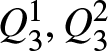 $Q_3^1, Q_3^2$ are the trilinear forms on
 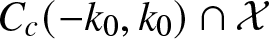 $C_c(-k_0,k_0) \cap \mathcal{X}$ defined by
 \begin{align*}
Q_3^1\big(\widehat{V}, \widehat{W},\widehat{Z}\big)(k) &= \sum_{j \in \left\lbrace -1,1 \right\rbrace^3} \int_\mathbb{R} \frac{P_{j_0}(k)}{\phi^2_{j}(k, l)} N_2(k, l)\big(P_{j_1} \chi B_2\big(\widehat{V}, \widehat{W}\big), P_{j_2}\widehat{Z}\big) \mathrm{d} l\\
Q_3^2\big(\widehat{V}, \widehat{W},\widehat{Z}\big)(k) &= \sum_{j \in \left\lbrace -1,1 \right\rbrace^3} \int_\mathbb{R} \frac{P_{j_0}(k)}{\phi^2_{j}(k, l)} N_2(k, l)\big(P_{j_1} \widehat{V}, P_{j_2} \chi B_2\big(\widehat{W}, \widehat{Z}\big)\big) \mathrm{d} l,
\end{align*}
\begin{align*}
Q_3^1\big(\widehat{V}, \widehat{W},\widehat{Z}\big)(k) &= \sum_{j \in \left\lbrace -1,1 \right\rbrace^3} \int_\mathbb{R} \frac{P_{j_0}(k)}{\phi^2_{j}(k, l)} N_2(k, l)\big(P_{j_1} \chi B_2\big(\widehat{V}, \widehat{W}\big), P_{j_2}\widehat{Z}\big) \mathrm{d} l\\
Q_3^2\big(\widehat{V}, \widehat{W},\widehat{Z}\big)(k) &= \sum_{j \in \left\lbrace -1,1 \right\rbrace^3} \int_\mathbb{R} \frac{P_{j_0}(k)}{\phi^2_{j}(k, l)} N_2(k, l)\big(P_{j_1} \widehat{V}, P_{j_2} \chi B_2\big(\widehat{W}, \widehat{Z}\big)\big) \mathrm{d} l,
\end{align*}and satisfying the estimate
 \begin{equation}
\big\|\partial_k^j Q_3^i\big(\widehat{V}, \widehat{W},\widehat{Z}\big)\big\|_{L^\infty} \lesssim \big\|{\widehat{V}}\big\|_{W^{j,1}}\big\|{\widehat{W}}\big\|_{L^\infty}\big\|\widehat{Z}\big\|_{L^1},
\end{equation}
\begin{equation}
\big\|\partial_k^j Q_3^i\big(\widehat{V}, \widehat{W},\widehat{Z}\big)\big\|_{L^\infty} \lesssim \big\|{\widehat{V}}\big\|_{W^{j,1}}\big\|{\widehat{W}}\big\|_{L^\infty}\big\|\widehat{Z}\big\|_{L^1},
\end{equation}for 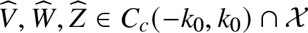 ${\widehat{V}},{\widehat{W}},\widehat{Z} \in C_c(-k_0,k_0) \cap \mathcal{X}$,
  $i = 1,2$ and
  $j = 0,1$ (with
  $j = 0$ in case
  $\mathcal{X} = Y_0$). In addition,
  $Q_2\big(\widehat{V},\widehat{V}\big)(0)$ is real for
  ${\widehat{V}} \in C_c(-k_0,k_0)$ satisfying
  $\smash{\overline{{\widehat{V}}(k)} = {\widehat{V}}(-k)}$ for
  $k \in (-k_0,k_0)$. Finally, there exists a
  $t$-independent constant
  $C \gt 0$ such that, if we have
  $t \in [0,T_{\max})$ with
  $\|\widehat{U}(t)\|_{L^1 \cap L^\infty} \leq 1$, then the remainder
  $\mathcal{E}_2(\cdot,t)$ can be bounded as
 \begin{align*}
\left\|\partial_k^j\left(\chi \mathcal{E}_2(\cdot,t)\right)\right\|_{L^\infty} &\leq C \big\|\widehat{U}(t)\big\|_{W^{j,1}} \big\|\widehat{U}(t)\big\|_{L^1} \left(\big\|\widehat{U}_\mathrm{s}(t)\big\|_{L^\infty} + \big\|\widehat{U}(t)\big\|_{L^1}\right),
\end{align*}
\begin{align*}
\left\|\partial_k^j\left(\chi \mathcal{E}_2(\cdot,t)\right)\right\|_{L^\infty} &\leq C \big\|\widehat{U}(t)\big\|_{W^{j,1}} \big\|\widehat{U}(t)\big\|_{L^1} \left(\big\|\widehat{U}_\mathrm{s}(t)\big\|_{L^\infty} + \big\|\widehat{U}(t)\big\|_{L^1}\right),
\end{align*}for  $j = 0,1$ (with
  $j = 0$ in case
  $\mathcal{X} = Y_0$).
Proof. We start by isolating the critical quadratic term in the nonlinearity in Equation (5.8) for  $\widehat{U}_\mathrm{c}$. Thus, suppressing the
  $t$-dependency of
  $\widehat{U}_\mathrm{s}$ and
  $\widehat{U}_\mathrm{c}$, we write
 \begin{equation}
\chi \mathcal{F} \mathcal{N}\big(\mathcal{F}^{-1}\big(\widehat{U}_\mathrm{c} + \widehat{U}_\mathrm{s}\big)\big) = \chi B_2\big(\widehat{U}_\mathrm{c},\widehat{U}_\mathrm{c}\big) + \chi R_2\big(\widehat{U}_\mathrm{c},\widehat{U}_\mathrm{s}\big),
\end{equation}
\begin{equation}
\chi \mathcal{F} \mathcal{N}\big(\mathcal{F}^{-1}\big(\widehat{U}_\mathrm{c} + \widehat{U}_\mathrm{s}\big)\big) = \chi B_2\big(\widehat{U}_\mathrm{c},\widehat{U}_\mathrm{c}\big) + \chi R_2\big(\widehat{U}_\mathrm{c},\widehat{U}_\mathrm{s}\big),
\end{equation}where we denote
 \begin{align*}
R_2\big(\widehat{U}_\mathrm{c},\widehat{U}_\mathrm{s}\big) &= 2B_2\big(\widehat{U}_\mathrm{c},\widehat{U}_\mathrm{s}\big) + B_2\big(\widehat{U}_\mathrm{s},\widehat{U}_\mathrm{s}\big) + \mathcal{F} \mathcal{R}_2\left(\mathcal{F}^{-1}\big(\widehat{U}_\mathrm{c} + \widehat{U}_\mathrm{s}\big)\right),
\end{align*}
\begin{align*}
R_2\big(\widehat{U}_\mathrm{c},\widehat{U}_\mathrm{s}\big) &= 2B_2\big(\widehat{U}_\mathrm{c},\widehat{U}_\mathrm{s}\big) + B_2\big(\widehat{U}_\mathrm{s},\widehat{U}_\mathrm{s}\big) + \mathcal{F} \mathcal{R}_2\left(\mathcal{F}^{-1}\big(\widehat{U}_\mathrm{c} + \widehat{U}_\mathrm{s}\big)\right),
\end{align*}with  $\mathcal{R}_2(V)$ defined by (6.7). Combining (6.5) and (6.8), yields a
  $t$-independent constant
  $C \gt 0$ such that, if we have
  $t \in [0,T_{\max})$ with
  $\|\widehat{U}(t)\|_{L^1 \cap L^\infty} \leq 1$, then it holds
 \begin{equation}
\begin{aligned}
\big\|\partial_k^j R_2\big(\widehat{U}_\mathrm{c}(t),\widehat{U}_\mathrm{s}(t)\big)\big\|_{L^\infty} &\leq C\big\|\widehat{U}(t)\big\|_{W^{j,1}}\left(\big\|\widehat{U}_\mathrm{s}(t)\big\|_{L^\infty} + \big\|\widehat{U}(t)\big\|_{L^1} \right),
\end{aligned}
\end{equation}
\begin{equation}
\begin{aligned}
\big\|\partial_k^j R_2\big(\widehat{U}_\mathrm{c}(t),\widehat{U}_\mathrm{s}(t)\big)\big\|_{L^\infty} &\leq C\big\|\widehat{U}(t)\big\|_{W^{j,1}}\left(\big\|\widehat{U}_\mathrm{s}(t)\big\|_{L^\infty} + \big\|\widehat{U}(t)\big\|_{L^1} \right),
\end{aligned}
\end{equation}for  $j = 0,1$.
Next, we rewrite the critical quadratic term (6.2) using integration by parts with respect to time. Firstly, we recall that the spectral projections  $P_\pm(k)$ of
  $\hat{\Lambda}(k)$ are well-defined on the interval
  $(-k_0,k_0)$ on which
  $\widehat{U}_\mathrm{c}(t)$ is supported. Thus, we can decompose (6.2) into
 \begin{equation}
\begin{aligned}
&\int_0^t \chi(k) \mathrm{e}^{\hat{\Lambda}(k) (t-s)} B_2\big(\widehat{U}_\mathrm{c}(s), \widehat{U}_\mathrm{c}(s)\big)(k) \, \mathrm{d} s \\
&\quad \ = \sum_{j \in \left\lbrace -1,1 \right\rbrace^3} \int_0^t \mathrm{e}^{\lambda_{j_0}(k)(t-s)} \chi(k) P_{j_0}(k) \int_\mathbb{R} N_2(k,l)\big(P_{j_1} \widehat{U}_\mathrm{c}(s), P_{j_2}\widehat{U}_\mathrm{c}(s)\big) \mathrm{d} l \mathrm{d} s,
\end{aligned}
\end{equation}
\begin{equation}
\begin{aligned}
&\int_0^t \chi(k) \mathrm{e}^{\hat{\Lambda}(k) (t-s)} B_2\big(\widehat{U}_\mathrm{c}(s), \widehat{U}_\mathrm{c}(s)\big)(k) \, \mathrm{d} s \\
&\quad \ = \sum_{j \in \left\lbrace -1,1 \right\rbrace^3} \int_0^t \mathrm{e}^{\lambda_{j_0}(k)(t-s)} \chi(k) P_{j_0}(k) \int_\mathbb{R} N_2(k,l)\big(P_{j_1} \widehat{U}_\mathrm{c}(s), P_{j_2}\widehat{U}_\mathrm{c}(s)\big) \mathrm{d} l \mathrm{d} s,
\end{aligned}
\end{equation}with  $k \in \mathbb{R}$ and
  $t \in [0,T_{\max})$. We will integrate by parts in each summand of (7.6) by integrating the exponential
  $\smash{\mathrm{e}^{\lambda_{j_0}(k)(t-s)}}$ and differentiating the quadratic contribution
 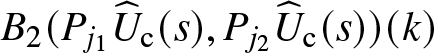 $B_2(P_{j_1} \widehat{U}_\mathrm{c}(s), P_{j_2}\widehat{U}_\mathrm{c}(s))(k)$ with respect to
  $s$. Thus, expressing the derivative
  $\partial_s \widehat{U}_\mathrm{c}(s)$ using Equation (5.8), recalling the expansion (7.4) and noting that
  $\hat{\Lambda}(k) P_{j_i}(k) = \lambda_{j_i}(k) P_{j_i}(k)$ for
  $i = 1,2$, we compute
 \begin{equation}
\begin{aligned}
&\partial_s N_2(k,l) \big(P_{j_1} \widehat{U}_\mathrm{c}, P_{j_2} \widehat{U}_\mathrm{c}\big)\\
&\quad\ = N_2(k,l) \big(P_{j_1} \partial_s \widehat{U}_\mathrm{c}, P_{j_2} \widehat{U}_\mathrm{c}\big) + N_2(k,l) \big(P_{j_1} \widehat{U}_\mathrm{c}, P_{j_2} \partial_s \widehat{U}_\mathrm{c}\big)\\
&\quad\ = \big(\lambda_{j_1}(k-l) + \lambda_{j_2}(l)\big) N_2(k,l)\big(P_{j_1}\widehat{U}_\mathrm{c}, P_{j_2}\widehat{U}_\mathrm{c}\big)\\
&\quad\ \qquad + \, N_2(k,l)\big(\chi P_{j_1} B_2\big(\widehat{U}_\mathrm{c}, \widehat{U}_\mathrm{c}\big), P_{j_2} \widehat{U}_\mathrm{c}\big) + N_2(k,l)\big(P_{j_1} \widehat{U}_\mathrm{c}, \chi P_{j_2} B_2\big(\widehat{U}_\mathrm{c}, \widehat{U}_\mathrm{c}\big)\big) \\
&\quad\ \qquad + \, N_2(k,l)\big(\chi P_{j_1} R_2\big(\widehat{U}_\mathrm{c}, \widehat{U}_\mathrm{s}\big), P_{j_2} \widehat{U}_\mathrm{c}\big) + N_2(k,l)\big(P_{j_1} \widehat{U}_\mathrm{c}, \chi P_{j_2} R_2\big(\widehat{U}_\mathrm{c},\widehat{U}_\mathrm{s}\big)\big),
\end{aligned}
\end{equation}
\begin{equation}
\begin{aligned}
&\partial_s N_2(k,l) \big(P_{j_1} \widehat{U}_\mathrm{c}, P_{j_2} \widehat{U}_\mathrm{c}\big)\\
&\quad\ = N_2(k,l) \big(P_{j_1} \partial_s \widehat{U}_\mathrm{c}, P_{j_2} \widehat{U}_\mathrm{c}\big) + N_2(k,l) \big(P_{j_1} \widehat{U}_\mathrm{c}, P_{j_2} \partial_s \widehat{U}_\mathrm{c}\big)\\
&\quad\ = \big(\lambda_{j_1}(k-l) + \lambda_{j_2}(l)\big) N_2(k,l)\big(P_{j_1}\widehat{U}_\mathrm{c}, P_{j_2}\widehat{U}_\mathrm{c}\big)\\
&\quad\ \qquad + \, N_2(k,l)\big(\chi P_{j_1} B_2\big(\widehat{U}_\mathrm{c}, \widehat{U}_\mathrm{c}\big), P_{j_2} \widehat{U}_\mathrm{c}\big) + N_2(k,l)\big(P_{j_1} \widehat{U}_\mathrm{c}, \chi P_{j_2} B_2\big(\widehat{U}_\mathrm{c}, \widehat{U}_\mathrm{c}\big)\big) \\
&\quad\ \qquad + \, N_2(k,l)\big(\chi P_{j_1} R_2\big(\widehat{U}_\mathrm{c}, \widehat{U}_\mathrm{s}\big), P_{j_2} \widehat{U}_\mathrm{c}\big) + N_2(k,l)\big(P_{j_1} \widehat{U}_\mathrm{c}, \chi P_{j_2} R_2\big(\widehat{U}_\mathrm{c},\widehat{U}_\mathrm{s}\big)\big),
\end{aligned}
\end{equation}for  $k, l \in \mathbb{R}$ and
  $j \in \left\lbrace -1,1 \right\rbrace^3$, where we have suppressed the
  $s$-dependency of
  $\widehat{U}_\mathrm{s}$ and
  $\widehat{U}_\mathrm{c}$. Since it holds
  $\phi_j^2(0,0) \in \{\pm \mathrm{i}\}$ for all
  $j\in \left\lbrace -1,1 \right\rbrace^3$, the phase function
  $\phi_j^2$ does not vanish on the square
  $[-k_0,k_0]^2$, upon taking
  $k_0 \gt 0$ smaller if necessary. Hence, using integration by parts, we obtain
 \begin{align*}
&\int_0^t \mathrm{e}^{\lambda_{j_0}(k)(t-s)} \int_\mathbb{R} \chi(k) P_{j_0}(k) N_2(k, l)\big(P_{j_1} \widehat{U}_\mathrm{c}(s), P_{j_2}\widehat{U}_\mathrm{c}(s)\big) \mathrm{d} l \mathrm{d} s\\
&\quad \ = \int_0^t \mathrm{e}^{\lambda_{j_0}(k)(t-s)} \int_\mathbb{R} \chi(k) \frac{\lambda_{j_0}(k)}{\phi_j^2(k,l)} P_{j_0}(k) N_2(k, l)\big(P_{j_1} \widehat{U}_\mathrm{c}(s), P_{j_2}\widehat{U}_\mathrm{c}(s)\big) \mathrm{d} l \mathrm{d} s\\
&\quad \ \qquad - \, \int_0^t \mathrm{e}^{\lambda_{j_0}(k)(t-s)} \int_\mathbb{R} \chi(k)\frac{\lambda_{j_1}(k-l) + \lambda_{j_2}(l)}{\phi_j^2(k,l)} P_{j_0}(k) N_2(k, l)\big(P_{j_1} \widehat{U}_\mathrm{c}(s), P_{j_2}\widehat{U}_\mathrm{c}(s)\big) \mathrm{d} l \mathrm{d} s \\
&\quad \ = -\left[\mathrm{e}^{\lambda_{j_0}(k)(t-s)} \int_\mathbb{R} \frac{\chi(k) }{\phi_j^2(k,l)} P_{j_0}(k) N_2(k, l)\big(P_{j_1} \widehat{U}_\mathrm{c}(s), P_{j_2}\widehat{U}_\mathrm{c}(s)\big) \mathrm{d} l \right]_{s = 0}^t\\
&\quad \ \qquad + \, \int_0^t \mathrm{e}^{\lambda_{j_0}(k)(t-s)} \int_\mathbb{R} \frac{\chi(k)}{\phi_j^2(k,l)} P_{j_0}(k) \partial_s N_2(k, l)\big(P_{j_1} \widehat{U}_\mathrm{c}(s), P_{j_2}\widehat{U}_\mathrm{c}(s)\big) \mathrm{d} l \mathrm{d} s\\
&\quad \ \qquad - \, \int_0^t \mathrm{e}^{\lambda_{j_0}(k)(t-s)} \int_\mathbb{R} \chi(k) P_{j_0}(k) \frac{\lambda_{j_1}(k-l) + \lambda_{j_2}(l)}{\phi_j^2(k,l)} N_2(k, l)\big(P_{j_1} \widehat{U}_\mathrm{c}(s), P_{j_2}\widehat{U}_\mathrm{c}(s)\big) \mathrm{d} l \mathrm{d} s
\end{align*}
\begin{align*}
&\int_0^t \mathrm{e}^{\lambda_{j_0}(k)(t-s)} \int_\mathbb{R} \chi(k) P_{j_0}(k) N_2(k, l)\big(P_{j_1} \widehat{U}_\mathrm{c}(s), P_{j_2}\widehat{U}_\mathrm{c}(s)\big) \mathrm{d} l \mathrm{d} s\\
&\quad \ = \int_0^t \mathrm{e}^{\lambda_{j_0}(k)(t-s)} \int_\mathbb{R} \chi(k) \frac{\lambda_{j_0}(k)}{\phi_j^2(k,l)} P_{j_0}(k) N_2(k, l)\big(P_{j_1} \widehat{U}_\mathrm{c}(s), P_{j_2}\widehat{U}_\mathrm{c}(s)\big) \mathrm{d} l \mathrm{d} s\\
&\quad \ \qquad - \, \int_0^t \mathrm{e}^{\lambda_{j_0}(k)(t-s)} \int_\mathbb{R} \chi(k)\frac{\lambda_{j_1}(k-l) + \lambda_{j_2}(l)}{\phi_j^2(k,l)} P_{j_0}(k) N_2(k, l)\big(P_{j_1} \widehat{U}_\mathrm{c}(s), P_{j_2}\widehat{U}_\mathrm{c}(s)\big) \mathrm{d} l \mathrm{d} s \\
&\quad \ = -\left[\mathrm{e}^{\lambda_{j_0}(k)(t-s)} \int_\mathbb{R} \frac{\chi(k) }{\phi_j^2(k,l)} P_{j_0}(k) N_2(k, l)\big(P_{j_1} \widehat{U}_\mathrm{c}(s), P_{j_2}\widehat{U}_\mathrm{c}(s)\big) \mathrm{d} l \right]_{s = 0}^t\\
&\quad \ \qquad + \, \int_0^t \mathrm{e}^{\lambda_{j_0}(k)(t-s)} \int_\mathbb{R} \frac{\chi(k)}{\phi_j^2(k,l)} P_{j_0}(k) \partial_s N_2(k, l)\big(P_{j_1} \widehat{U}_\mathrm{c}(s), P_{j_2}\widehat{U}_\mathrm{c}(s)\big) \mathrm{d} l \mathrm{d} s\\
&\quad \ \qquad - \, \int_0^t \mathrm{e}^{\lambda_{j_0}(k)(t-s)} \int_\mathbb{R} \chi(k) P_{j_0}(k) \frac{\lambda_{j_1}(k-l) + \lambda_{j_2}(l)}{\phi_j^2(k,l)} N_2(k, l)\big(P_{j_1} \widehat{U}_\mathrm{c}(s), P_{j_2}\widehat{U}_\mathrm{c}(s)\big) \mathrm{d} l \mathrm{d} s
\end{align*}for  $k \in \mathbb{R}$,
  $t \in [0,T_{\max})$ and
  $j\in \left\lbrace -1,1 \right\rbrace^3$. So, taking the sum of the latter over all
  $j \in \left\lbrace -1,1 \right\rbrace^3$, we obtain the desired identity (7.1) by (7.6) and (7.7) with error function
 \begin{align*}
\mathcal{E}_2(k,t) &= \sum_{j \in \left\lbrace -1,1 \right\rbrace^3} \int_\mathbb{R} \frac{1}{\phi_j^2(k,l)} P_{j_0}(k) \left(
N_2(k,l)\big(\chi P_{j_1} R_2\big(\widehat{U}_\mathrm{c}(t), \widehat{U}_\mathrm{s}(t)\big), P_{j_2} \widehat{U}_\mathrm{c}\big)\right. \\
&\qquad \left. +\, N_2(k,l)\big(P_{j_1} \widehat{U}_\mathrm{c}(t), \chi P_{j_2} R_2\big(\widehat{U}_\mathrm{c}(t),\widehat{U}_\mathrm{s}(t)\big)\big)\right) \mathrm{d} l,
\end{align*}
\begin{align*}
\mathcal{E}_2(k,t) &= \sum_{j \in \left\lbrace -1,1 \right\rbrace^3} \int_\mathbb{R} \frac{1}{\phi_j^2(k,l)} P_{j_0}(k) \left(
N_2(k,l)\big(\chi P_{j_1} R_2\big(\widehat{U}_\mathrm{c}(t), \widehat{U}_\mathrm{s}(t)\big), P_{j_2} \widehat{U}_\mathrm{c}\big)\right. \\
&\qquad \left. +\, N_2(k,l)\big(P_{j_1} \widehat{U}_\mathrm{c}(t), \chi P_{j_2} R_2\big(\widehat{U}_\mathrm{c}(t),\widehat{U}_\mathrm{s}(t)\big)\big)\right) \mathrm{d} l,
\end{align*}for  $t \in [0,T_{\max})$. Applying Young’s convolution inequality, while using estimate (7.5) and recalling that the phase function
  $\phi_j^2$ is bounded away from
  $0$ on the square
  $[-k_0,k_0]^2$ and the cut-off function
  $\chi$ is supported on
  $(-k_0,k_0)$, we obtain
  $t$-independent constants
  $C_{1,2} \gt 0$ such that, if we have
  $t \in [0,T_{\max})$ with
  $\smash{\|\widehat{U}(t)\|_{L^1 \cap L^\infty}} \leq 1$, then it holds
 \begin{align*}
&\left\|\partial_k^j\left(\chi \mathcal{E}_2(\cdot,t)\right)\right\|_{L^\infty} \\
&\quad \ \leq C_1 \left(\big\|\widehat{U}_\mathrm{c}(t)\big\|_{L^1} \big\|R_2(\widehat{U}_\mathrm{c}(t),\widehat{U}_\mathrm{s}(t)\big\|_{W^{j,\infty}} + \big\|\widehat{U}_\mathrm{c}(t)\big\|_{W^{j,1}} \big\|R_2(\widehat{U}_\mathrm{c}(t),\widehat{U}_\mathrm{s}(t)\big\|_{L^\infty}\right) \\
&\quad \ \leq C_2 \big\|\widehat{U}(t)\big\|_{W^{j,1}} \big\|\widehat{U}(t)\big\|_{L^1} \left(\big\|\widehat{U}_\mathrm{s}(t)\big\|_{L^\infty} + \big\|\widehat{U}(t)\big\|_{L^1}\right),
\end{align*}
\begin{align*}
&\left\|\partial_k^j\left(\chi \mathcal{E}_2(\cdot,t)\right)\right\|_{L^\infty} \\
&\quad \ \leq C_1 \left(\big\|\widehat{U}_\mathrm{c}(t)\big\|_{L^1} \big\|R_2(\widehat{U}_\mathrm{c}(t),\widehat{U}_\mathrm{s}(t)\big\|_{W^{j,\infty}} + \big\|\widehat{U}_\mathrm{c}(t)\big\|_{W^{j,1}} \big\|R_2(\widehat{U}_\mathrm{c}(t),\widehat{U}_\mathrm{s}(t)\big\|_{L^\infty}\right) \\
&\quad \ \leq C_2 \big\|\widehat{U}(t)\big\|_{W^{j,1}} \big\|\widehat{U}(t)\big\|_{L^1} \left(\big\|\widehat{U}_\mathrm{s}(t)\big\|_{L^\infty} + \big\|\widehat{U}(t)\big\|_{L^1}\right),
\end{align*}for  $j = 0,1$ (with
  $j = 0$ in case
  $\mathcal{X} = Y_0$). Similarly, we derive the bounds (7.2) and (7.3).
Next, let  ${\widehat{V}} \in C_c(-k_0,k_0)$ with
  $\overline{{\widehat{V}}(k)} = {\widehat{V}}(-k)$ for
  $k \in \mathbb{R}$. We prove
  $Q_2({\widehat{V}},{\widehat{V}})(0) \in \mathbb{R}$. Firstly, we note that the maps
  $\tau, \xi \colon \left\lbrace -1,1 \right\rbrace^3 \to \left\lbrace -1,1 \right\rbrace^3$ given by
  $\tau(j_0,j_1,j_2) = (j_0,j_2,j_1)$ and
  $\xi(j) = -j$ are bijections. We have
 \begin{align*}
\phi_j^2(k,l) = \phi_{\tau(j)}^2(k,k-l),
\end{align*}
\begin{align*}
\phi_j^2(k,l) = \phi_{\tau(j)}^2(k,k-l),
\end{align*}for  $k,l \in \mathbb{R}$ and
  $j \in \left\lbrace -1,1 \right\rbrace^3$. Hence, using (4.3), we obtain
 \begin{align*}
\overline{Q_2({\widehat{V}},{\widehat{V}})(0)} &= \sum_{j \in \left\lbrace -1,1 \right\rbrace^3} \int_\mathbb{R} \frac{P_{-j_0}(0)}{\phi_{-j}^2(0,l)} N_2(0,l)\left(P_{-j_1} \overline{{\widehat{V}}}, P_{-j_2} \overline{{\widehat{V}}}\right) \mathrm{d} l\\
&= \sum_{j \in \left\lbrace -1,1 \right\rbrace^3} \int_\mathbb{R} \frac{P_{j_0}(0)}{\phi_{j}^2(0,l)} N_2(0,l)\left(P_{j_2} {\widehat{V}}, P_{j_1} {\widehat{V}} \right) \mathrm{d} l\\
&= \sum_{j \in \left\lbrace -1,1 \right\rbrace^3} \int_\mathbb{R} \frac{P_{\tau(j)_0}(0)}{\phi_{\tau(j)}^2(0,l)} N_2(0,l)\left(P_{\tau(j)_1} {\widehat{V}}, P_{\tau(j)_2} {\widehat{V}} \right) \mathrm{d} l\\
&= Q_2({\widehat{V}},{\widehat{V}})(0),
\end{align*}
\begin{align*}
\overline{Q_2({\widehat{V}},{\widehat{V}})(0)} &= \sum_{j \in \left\lbrace -1,1 \right\rbrace^3} \int_\mathbb{R} \frac{P_{-j_0}(0)}{\phi_{-j}^2(0,l)} N_2(0,l)\left(P_{-j_1} \overline{{\widehat{V}}}, P_{-j_2} \overline{{\widehat{V}}}\right) \mathrm{d} l\\
&= \sum_{j \in \left\lbrace -1,1 \right\rbrace^3} \int_\mathbb{R} \frac{P_{j_0}(0)}{\phi_{j}^2(0,l)} N_2(0,l)\left(P_{j_2} {\widehat{V}}, P_{j_1} {\widehat{V}} \right) \mathrm{d} l\\
&= \sum_{j \in \left\lbrace -1,1 \right\rbrace^3} \int_\mathbb{R} \frac{P_{\tau(j)_0}(0)}{\phi_{\tau(j)}^2(0,l)} N_2(0,l)\left(P_{\tau(j)_1} {\widehat{V}}, P_{\tau(j)_2} {\widehat{V}} \right) \mathrm{d} l\\
&= Q_2({\widehat{V}},{\widehat{V}})(0),
\end{align*}which implies  $Q_2({\widehat{V}},{\widehat{V}})(0) \in \mathbb{R}$.
8. Eliminating nonresonant cubic terms
In Proposition 7.1, we have expressed the critical quadratic term (6.2) in the Duhamel formula (5.10) of  $\widehat{U}_\mathrm{c}$ through integration by parts in time as a cubic integral term
 \begin{equation}
\int_0^t \chi(k) \mathrm{e}^{\hat{\Lambda}(k)(t-s)} \left(Q_3^1\big(\widehat{U}_\mathrm{c}(s), \widehat{U}_\mathrm{c}(s), \widehat{U}_\mathrm{c}(s)\big)(k) + Q_3^1\big(\widehat{U}_\mathrm{c}(s), \widehat{U}_\mathrm{c}(s), \widehat{U}_\mathrm{c}(s)\big)(k)\right) \mathrm{d} s,
\end{equation}
\begin{equation}
\int_0^t \chi(k) \mathrm{e}^{\hat{\Lambda}(k)(t-s)} \left(Q_3^1\big(\widehat{U}_\mathrm{c}(s), \widehat{U}_\mathrm{c}(s), \widehat{U}_\mathrm{c}(s)\big)(k) + Q_3^1\big(\widehat{U}_\mathrm{c}(s), \widehat{U}_\mathrm{c}(s), \widehat{U}_\mathrm{c}(s)\big)(k)\right) \mathrm{d} s,
\end{equation}a quadratic boundary term
 \begin{equation}
\begin{aligned}
\left[e^{\hat{\Lambda}(k)(t-s)} Q_2\big(\widehat{U}_\mathrm{c}(s), \widehat{U}_\mathrm{c}(s)\big)(k) \right]_0^t &= Q_2\big(\widehat{U}_\mathrm{c}(t), \widehat{U}_\mathrm{c}(t)\big)(k)\\
&\qquad - \, \mathrm{e}^{\hat{\Lambda}(k)t} Q_2\big(\widehat{U}_\mathrm{c}(0), \widehat{U}_\mathrm{c}(0)\big)(k),
\end{aligned}
\end{equation}
\begin{equation}
\begin{aligned}
\left[e^{\hat{\Lambda}(k)(t-s)} Q_2\big(\widehat{U}_\mathrm{c}(s), \widehat{U}_\mathrm{c}(s)\big)(k) \right]_0^t &= Q_2\big(\widehat{U}_\mathrm{c}(t), \widehat{U}_\mathrm{c}(t)\big)(k)\\
&\qquad - \, \mathrm{e}^{\hat{\Lambda}(k)t} Q_2\big(\widehat{U}_\mathrm{c}(0), \widehat{U}_\mathrm{c}(0)\big)(k),
\end{aligned}
\end{equation}and a remainder integral term
 \begin{equation}
\int_0^t \mathrm{e}^{\widehat{\Lambda}(k)(t-s)} \chi(k) \mathcal{E}_2(k,s) \mathrm{d} s.
\end{equation}
\begin{equation}
\int_0^t \mathrm{e}^{\widehat{\Lambda}(k)(t-s)} \chi(k) \mathcal{E}_2(k,s) \mathrm{d} s.
\end{equation} The right-hand side of the bound on  $\mathcal{E}_2(k,s)$ in Proposition 7.1 consists of terms which have a
  $\widehat{U}_\mathrm{s}$-contribution, or terms which are quartic in
  $\widehat{U}_\mathrm{c}$. Therefore, as argued before, the remainder integral term (8.3) can be controlled through standard
  $L^1$-
 $L^\infty$-estimates. Moreover, since the boundary term (8.2) is quadratic in
  $\widehat{U}_\mathrm{c}$, it necessarily decays at a higher rate than
  $\widehat{U}_\mathrm{c}$ itself. So, this boundary term is irrelevant and, thus, does not obstruct the nonlinear argument.
Therefore, the only remaining critical nonlinear terms in the Duhamel formulas (5.10)–(5.11) after applying Proposition 7.1 are the cubic terms (6.3) and (8.1). As for the critical quadratic term (6.2), we can exploit the oscillatory character in time of the integrals arising in (6.3) and (8.1) as long as the associated phase function is nonzero. We will establish that the phase functions  $\phi_j^3 \colon \mathbb{R}^3 \to \mathbb{R}$ associated with the cubic terms are given by
 \begin{align*}
\phi^3_{j}(k,l_1,l_2) = \lambda_{j_0}(k) - \lambda_{j_1}(k - l_1) - \lambda_{j_2}(l_1-l_2) - \lambda_{j_3}(l_2),
\end{align*}
\begin{align*}
\phi^3_{j}(k,l_1,l_2) = \lambda_{j_0}(k) - \lambda_{j_1}(k - l_1) - \lambda_{j_2}(l_1-l_2) - \lambda_{j_3}(l_2),
\end{align*}for  $j = (j_0,j_1,j_2,j_3) \in \left\lbrace -1, 1 \right\rbrace^4$. We identify the set of time resonances
  $\mathcal{T} \subset \left\lbrace -1,1 \right\rbrace^4$ as
 \begin{align*}
\mathcal{T} = \left\{j \in \left\lbrace -1,1 \right\rbrace^4 : j_0-j_1-j_2-j_3 = 0\right\},
\end{align*}
\begin{align*}
\mathcal{T} = \left\{j \in \left\lbrace -1,1 \right\rbrace^4 : j_0-j_1-j_2-j_3 = 0\right\},
\end{align*}and denote its complement by  $\mathcal{T}^c = \left\lbrace -1,1 \right\rbrace^4 \setminus \mathcal{T}$. That is, for
  $j \in \left\lbrace -1,1 \right\rbrace^4$ it holds
  $\phi^3_j(0,0,0) = 0$ if and only if
  $j \in \mathcal{T}$. Moreover, it holds
  $\nabla \phi^3_j(0,0,0) = 0$ for all
  $j \in \{-1,1\}^4$, showing that the cubic terms are all space-resonant at the critical frequency
  $k = 0$, cf. [Reference Germain15]. Splitting into time-resonant and time-nonresonant terms, the sum of the critical cubic integral terms (6.3) and (8.1) decomposes as
 \begin{equation}
\begin{aligned}
&\int_0^t \chi(k) \mathrm{e}^{\widehat{\Lambda}(k) (t-s)} Z_3\big(\widehat{U}_\mathrm{c}(s),\widehat{U}_\mathrm{c}(s),\widehat{U}_\mathrm{c}(s)\big)(k) \, \mathrm{d} s\\
&\quad \ = \int_0^t \chi(k) \mathrm{e}^{\widehat{\Lambda}(k) (t-s)} Z_3^{\mathrm{res}}\big(\widehat{U}_\mathrm{c}(s),\widehat{U}_\mathrm{c}(s),\widehat{U}_\mathrm{c}(s)\big)(k) \, \mathrm{d} s\\
&\quad \ \qquad + \, \int_0^t \chi(k) \mathrm{e}^{\widehat{\Lambda}(k) (t-s)} Z_3^{\mathrm{c}}\big(\widehat{U}_\mathrm{c}(s),\widehat{U}_\mathrm{c}(s),\widehat{U}_\mathrm{c}(s)\big)(k) \, \mathrm{d} s,
\end{aligned}
\end{equation}
\begin{equation}
\begin{aligned}
&\int_0^t \chi(k) \mathrm{e}^{\widehat{\Lambda}(k) (t-s)} Z_3\big(\widehat{U}_\mathrm{c}(s),\widehat{U}_\mathrm{c}(s),\widehat{U}_\mathrm{c}(s)\big)(k) \, \mathrm{d} s\\
&\quad \ = \int_0^t \chi(k) \mathrm{e}^{\widehat{\Lambda}(k) (t-s)} Z_3^{\mathrm{res}}\big(\widehat{U}_\mathrm{c}(s),\widehat{U}_\mathrm{c}(s),\widehat{U}_\mathrm{c}(s)\big)(k) \, \mathrm{d} s\\
&\quad \ \qquad + \, \int_0^t \chi(k) \mathrm{e}^{\widehat{\Lambda}(k) (t-s)} Z_3^{\mathrm{c}}\big(\widehat{U}_\mathrm{c}(s),\widehat{U}_\mathrm{c}(s),\widehat{U}_\mathrm{c}(s)\big)(k) \, \mathrm{d} s,
\end{aligned}
\end{equation}where  $Z_3, Z_3^{\mathrm{res}}, Z_3^{\mathrm{c}}$ are the trilinear forms on
  $C_c(-k_0,k_0) \cap \mathcal{X}$ given by
 \begin{equation}
\begin{aligned}
Z_3\big({\widehat{V}},{\widehat{W}},\widehat{Z}\big)(k) &= B_3\big({\widehat{V}},{\widehat{W}},\widehat{Z}\big)(k) + Q_3^1\big({\widehat{V}},{\widehat{W}},\widehat{Z}\big)(k) + Q_3^2\big({\widehat{V}},{\widehat{W}},\widehat{Z}\big)(k)\\
&= \int_\mathbb{R} \int_\mathbb{R} \widetilde{N}_3(k,l_1,l_2)\big({\widehat{V}},{\widehat{W}},\widehat{Z}\big)\mathrm{d} l_1 \mathrm{d} l_2,
\end{aligned}
\end{equation}
\begin{equation}
\begin{aligned}
Z_3\big({\widehat{V}},{\widehat{W}},\widehat{Z}\big)(k) &= B_3\big({\widehat{V}},{\widehat{W}},\widehat{Z}\big)(k) + Q_3^1\big({\widehat{V}},{\widehat{W}},\widehat{Z}\big)(k) + Q_3^2\big({\widehat{V}},{\widehat{W}},\widehat{Z}\big)(k)\\
&= \int_\mathbb{R} \int_\mathbb{R} \widetilde{N}_3(k,l_1,l_2)\big({\widehat{V}},{\widehat{W}},\widehat{Z}\big)\mathrm{d} l_1 \mathrm{d} l_2,
\end{aligned}
\end{equation}and
 \begin{equation}
\begin{aligned}
Z_3^{\mathrm{res}}\big({\widehat{V}},{\widehat{W}},\widehat{Z}\big) &= \sum_{j \in \mathcal{T}} P_{j_0}(k) Z_3\big(P_{j_1} {\widehat{V}}, P_{j_2} {\widehat{W}}, P_{j_3} \widehat{Z}\big),\\
Z_3^{\mathrm{c}}\big({\widehat{V}},{\widehat{W}},\widehat{Z}\big) &= \sum_{j \in \mathcal{T}^c} P_{j_0}(k) Z_3\big(P_{j_1} {\widehat{V}}, P_{j_2} {\widehat{W}}, P_{j_3} \widehat{Z}\big),
\end{aligned}
\end{equation}
\begin{equation}
\begin{aligned}
Z_3^{\mathrm{res}}\big({\widehat{V}},{\widehat{W}},\widehat{Z}\big) &= \sum_{j \in \mathcal{T}} P_{j_0}(k) Z_3\big(P_{j_1} {\widehat{V}}, P_{j_2} {\widehat{W}}, P_{j_3} \widehat{Z}\big),\\
Z_3^{\mathrm{c}}\big({\widehat{V}},{\widehat{W}},\widehat{Z}\big) &= \sum_{j \in \mathcal{T}^c} P_{j_0}(k) Z_3\big(P_{j_1} {\widehat{V}}, P_{j_2} {\widehat{W}}, P_{j_3} \widehat{Z}\big),
\end{aligned}
\end{equation}with
 \begin{equation*}
\begin{aligned}
&\widetilde{N}_3(k,l_1,l_2)\big({\widehat{V}},{\widehat{W}},\widehat{Z}\big) \\
&\quad \ = N_3(k,l_1,l_2)\big({\widehat{V}},{\widehat{W}},\widehat{Z}\big) + \sum_{j \in \left\lbrace -1,1 \right\rbrace^3} \frac{P_{j_0}(k)}{\phi^2_{j}(k,l_2)} N_2(k,l_2)\big(\chi P_{j_1} N_2(\cdot,l_1-l_2) \big(\widehat{V}, \widehat{W}\big), P_{j_2}\widehat{Z}\big)\\
&\quad \ \qquad + \, \sum_{j \in \left\lbrace -1,1 \right\rbrace^3} \frac{P_{j_0}(k)}{\phi^2_{j}(k,l_1)} N_2(k,l_1)\big(P_{j_1} \widehat{V}, \chi P_{j_2} N_2(\cdot,l_2)\big(\widehat{W}, \widehat{Z}\big)\big).
\end{aligned}
\end{equation*}
\begin{equation*}
\begin{aligned}
&\widetilde{N}_3(k,l_1,l_2)\big({\widehat{V}},{\widehat{W}},\widehat{Z}\big) \\
&\quad \ = N_3(k,l_1,l_2)\big({\widehat{V}},{\widehat{W}},\widehat{Z}\big) + \sum_{j \in \left\lbrace -1,1 \right\rbrace^3} \frac{P_{j_0}(k)}{\phi^2_{j}(k,l_2)} N_2(k,l_2)\big(\chi P_{j_1} N_2(\cdot,l_1-l_2) \big(\widehat{V}, \widehat{W}\big), P_{j_2}\widehat{Z}\big)\\
&\quad \ \qquad + \, \sum_{j \in \left\lbrace -1,1 \right\rbrace^3} \frac{P_{j_0}(k)}{\phi^2_{j}(k,l_1)} N_2(k,l_1)\big(P_{j_1} \widehat{V}, \chi P_{j_2} N_2(\cdot,l_2)\big(\widehat{W}, \widehat{Z}\big)\big).
\end{aligned}
\end{equation*}Using the same strategy as in the proof of Proposition 7.1, we express the nonresonant part of the critical cubic term (8.4) as a cubic boundary term and a quartic remainder through integration by parts in time. We arrive at the following result.
Proposition 8.1. The nonresonant part of the critical cubic term (8.4) can be expressed as
 \begin{equation}
\begin{aligned}
&\int_0^t \chi(k) \mathrm{e}^{\widehat{\Lambda}(k) (t-s)} Z_3^{\mathrm{c}}\big(\widehat{U}_\mathrm{c}(s),\widehat{U}_\mathrm{c}(s),\widehat{U}_\mathrm{c}(s)\big)(k) \, \mathrm{d} s \\
&\quad \ = \int_0^t \mathrm{e}^{\widehat{\Lambda}(k)(t-s)} \chi(k) \mathcal{E}_3(k,s) \mathrm{d} s - \left[e^{\hat{\Lambda}(k)(t-s)} K_3\big(\widehat{U}_\mathrm{c}(s), \widehat{U}_\mathrm{c}(s),\widehat{U}_\mathrm{c}(s)\big)(k) \right]_0^t,
\end{aligned}
\end{equation}
\begin{equation}
\begin{aligned}
&\int_0^t \chi(k) \mathrm{e}^{\widehat{\Lambda}(k) (t-s)} Z_3^{\mathrm{c}}\big(\widehat{U}_\mathrm{c}(s),\widehat{U}_\mathrm{c}(s),\widehat{U}_\mathrm{c}(s)\big)(k) \, \mathrm{d} s \\
&\quad \ = \int_0^t \mathrm{e}^{\widehat{\Lambda}(k)(t-s)} \chi(k) \mathcal{E}_3(k,s) \mathrm{d} s - \left[e^{\hat{\Lambda}(k)(t-s)} K_3\big(\widehat{U}_\mathrm{c}(s), \widehat{U}_\mathrm{c}(s),\widehat{U}_\mathrm{c}(s)\big)(k) \right]_0^t,
\end{aligned}
\end{equation}for  $k \in \mathbb{R}$ and
  $t \in [0,T_{\max})$, where
  $K_3$ is the trilinear form on
  $C_c(-k_0,k_0) \cap \mathcal{X}$ defined by
 \begin{align*}
K_3\big(\widehat{V}, \widehat{W}, \widehat{Z}\big)(k) = \sum_{j \in \mathcal{T}^c} \int_\mathbb{R} \int_\mathbb{R} \frac{\chi(k) P_{j_0}(k)}{\phi^3_j(k, l_1,l_2)} \widetilde{N}_3(k,l_1,l_2)\big(P_{j_1} \widehat{V}, P_{j_2}\widehat{W}, P_{j_3} \widehat{Z}\big) \mathrm{d} l_1 \mathrm{d} l_2,
\end{align*}
\begin{align*}
K_3\big(\widehat{V}, \widehat{W}, \widehat{Z}\big)(k) = \sum_{j \in \mathcal{T}^c} \int_\mathbb{R} \int_\mathbb{R} \frac{\chi(k) P_{j_0}(k)}{\phi^3_j(k, l_1,l_2)} \widetilde{N}_3(k,l_1,l_2)\big(P_{j_1} \widehat{V}, P_{j_2}\widehat{W}, P_{j_3} \widehat{Z}\big) \mathrm{d} l_1 \mathrm{d} l_2,
\end{align*}and obeying the bound
 \begin{equation}
\big\|\partial_k^j K_3\big({\widehat{V}},{\widehat{W}},\widehat{Z}\big)\big\|_{L^p} \lesssim \big\|{\widehat{V}}\big\|_{W^{j,1}} \big\|{\widehat{W}}\big\|_{L^p} \big\|\widehat{Z}\big\|_{L^1},
\end{equation}
\begin{equation}
\big\|\partial_k^j K_3\big({\widehat{V}},{\widehat{W}},\widehat{Z}\big)\big\|_{L^p} \lesssim \big\|{\widehat{V}}\big\|_{W^{j,1}} \big\|{\widehat{W}}\big\|_{L^p} \big\|\widehat{Z}\big\|_{L^1},
\end{equation}for  ${\widehat{V}},{\widehat{W}},\widehat{Z} \in C_c(-k_0,k_0) \cap \mathcal{X}$,
  $p = 1,\infty$ and
  $j = 0,1$ (with
  $j = 0$ in case
  $\mathcal{X} = Y_0$). In addition,
  $K_3\big({\widehat{V}},{\widehat{V}},{\widehat{V}}\big)(0)$ is real for
  ${\widehat{V}} \in C_c(-k_0,k_0)$ satisfying
  $\smash{\overline{{\widehat{V}}(k)} = {\widehat{V}}(-k)}$ for
  $k \in \mathbb{R}$. Finally, there exists a
  $t$-independent constant
  $C \gt 0$ such that, if we have
  $t \in [0,T_{\max})$ with
  $\|\widehat{U}(t)\|_{L^1} \leq 1$, then the remainder
  $\mathcal{E}_3(\cdot,t)$ can be bounded as
 \begin{align*}
\left\|\partial_k^j\left(\chi \mathcal{E}_3(\cdot,t)\right)\right\|_{L^\infty} &\leq C \big\|\widehat{U}(t)\big\|_{L^1}^2 \big\|\widehat{U}(t)\big\|_{W^{j,1}} \big\|\widehat{U}(t)\big\|_{L^\infty},
\end{align*}
\begin{align*}
\left\|\partial_k^j\left(\chi \mathcal{E}_3(\cdot,t)\right)\right\|_{L^\infty} &\leq C \big\|\widehat{U}(t)\big\|_{L^1}^2 \big\|\widehat{U}(t)\big\|_{W^{j,1}} \big\|\widehat{U}(t)\big\|_{L^\infty},
\end{align*}for  $j = 0,1$ (with
  $j = 0$ in case
  $\mathcal{X} = Y_0$).
Proof. We integrate by parts in each summand of
 \begin{equation}
\begin{aligned}
&\int_0^t \chi(k) \mathrm{e}^{\widehat{\Lambda}(k) (t-s)} Z_3^{\mathrm{c}}\big(\widehat{U}_\mathrm{c}(s),\widehat{U}_\mathrm{c}(s),\widehat{U}_\mathrm{c}(s)\big)(k) \, \mathrm{d} s\\
&\quad \ =
\sum_{j \in \mathcal{T}^c} \int_0^t \chi(k) \mathrm{e}^{\lambda_0(k) (t-s)} P_{j_0}(k) Z_3\big(P_{j_1} \widehat{U}_\mathrm{c}(s), P_{j_2} \widehat{U}_\mathrm{c}(s), P_{j_3} \widehat{U}_\mathrm{c}(s)\big)(k) \, \mathrm{d} s\\
&\quad \ =
\sum_{j \in \mathcal{T}^c} \int_0^t \chi(k) \mathrm{e}^{\lambda_0(k) (t-s)}P_{j_0}(k) \int_\mathbb{R}\int_\mathbb{R} \widetilde{K}_j(k,l_1,l_2,s) \mathrm{d} l_1 \mathrm{d} l_2 \mathrm{d} s,
\end{aligned}
\end{equation}
\begin{equation}
\begin{aligned}
&\int_0^t \chi(k) \mathrm{e}^{\widehat{\Lambda}(k) (t-s)} Z_3^{\mathrm{c}}\big(\widehat{U}_\mathrm{c}(s),\widehat{U}_\mathrm{c}(s),\widehat{U}_\mathrm{c}(s)\big)(k) \, \mathrm{d} s\\
&\quad \ =
\sum_{j \in \mathcal{T}^c} \int_0^t \chi(k) \mathrm{e}^{\lambda_0(k) (t-s)} P_{j_0}(k) Z_3\big(P_{j_1} \widehat{U}_\mathrm{c}(s), P_{j_2} \widehat{U}_\mathrm{c}(s), P_{j_3} \widehat{U}_\mathrm{c}(s)\big)(k) \, \mathrm{d} s\\
&\quad \ =
\sum_{j \in \mathcal{T}^c} \int_0^t \chi(k) \mathrm{e}^{\lambda_0(k) (t-s)}P_{j_0}(k) \int_\mathbb{R}\int_\mathbb{R} \widetilde{K}_j(k,l_1,l_2,s) \mathrm{d} l_1 \mathrm{d} l_2 \mathrm{d} s,
\end{aligned}
\end{equation}where we abbreviate
 \begin{align*}
\widetilde{K}_j(k,l_1,l_2,s) &= \widetilde{N}_3(k,l_1,l_2)\big(P_{j_1} \widehat{U}_\mathrm{c}(s), P_{j_2}\widehat{U}_\mathrm{c}(s),P_{j_3}\widehat{U}_\mathrm{c}(s)\big).
\end{align*}
\begin{align*}
\widetilde{K}_j(k,l_1,l_2,s) &= \widetilde{N}_3(k,l_1,l_2)\big(P_{j_1} \widehat{U}_\mathrm{c}(s), P_{j_2}\widehat{U}_\mathrm{c}(s),P_{j_3}\widehat{U}_\mathrm{c}(s)\big).
\end{align*} We express the derivative  $\partial_s \widehat{U}_\mathrm{c}(s)$ through Equation (5.8) and note that
 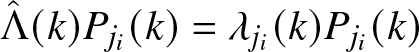 $\hat{\Lambda}(k) P_{j_i}(k) = \lambda_{j_i}(k) P_{j_i}(k)$ for
 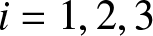 $i = 1,2,3$, which leads to
 \begin{equation}
\begin{aligned}
&\partial_s \widetilde{K}_j(k,l_1,l_2,s)\\
&\quad \ = \widetilde{N}_3(k,l_1,l_2) \big(P_{j_1} \partial_s \widehat{U}_\mathrm{c}, P_{j_2} \widehat{U}_\mathrm{c},P_{j_3} \widehat{U}_\mathrm{c}\big) + \widetilde{N}_3(k,l_1,l_2) \big(P_{j_1} \widehat{U}_\mathrm{c}, P_{j_2} \partial_s \widehat{U}_\mathrm{c},P_{j_3} \widehat{U}_\mathrm{c}\big)\\ &\quad \ \qquad + \, \widetilde{N}_3(k,l_1,l_2) \big(P_{j_1} \widehat{U}_\mathrm{c}, P_{j_2} \widehat{U}_\mathrm{c},P_{j_3} \partial_s \widehat{U}_\mathrm{c}\big) \\
&\quad \ = \big(\lambda_{j_1}(k-l_1) + \lambda_{j_2}(l_1-l_2) + \lambda_{j_3}(l_2)\big) \widetilde{K}_j(k,l_1,l_2,s) + \check{K}_j(k,l_1,l_2,s),
\end{aligned}
\end{equation}
\begin{equation}
\begin{aligned}
&\partial_s \widetilde{K}_j(k,l_1,l_2,s)\\
&\quad \ = \widetilde{N}_3(k,l_1,l_2) \big(P_{j_1} \partial_s \widehat{U}_\mathrm{c}, P_{j_2} \widehat{U}_\mathrm{c},P_{j_3} \widehat{U}_\mathrm{c}\big) + \widetilde{N}_3(k,l_1,l_2) \big(P_{j_1} \widehat{U}_\mathrm{c}, P_{j_2} \partial_s \widehat{U}_\mathrm{c},P_{j_3} \widehat{U}_\mathrm{c}\big)\\ &\quad \ \qquad + \, \widetilde{N}_3(k,l_1,l_2) \big(P_{j_1} \widehat{U}_\mathrm{c}, P_{j_2} \widehat{U}_\mathrm{c},P_{j_3} \partial_s \widehat{U}_\mathrm{c}\big) \\
&\quad \ = \big(\lambda_{j_1}(k-l_1) + \lambda_{j_2}(l_1-l_2) + \lambda_{j_3}(l_2)\big) \widetilde{K}_j(k,l_1,l_2,s) + \check{K}_j(k,l_1,l_2,s),
\end{aligned}
\end{equation}for 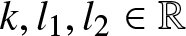 $k, l_1,l_2 \in \mathbb{R}$ and
 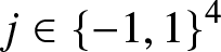 $j \in \left\lbrace -1,1 \right\rbrace^4$, where we have suppressed the
  $s$-dependency of
  $\widehat{U}_\mathrm{s}$ and
  $\widehat{U}_\mathrm{c}$ and we denote
 \begin{align*}
\check{K}_j(k,l_1,l_2,s) &=
\widetilde{N}_3(k,l_1,l_2)\big(\chi P_{j_1} \mathcal{F} \mathcal{N} \big(\mathcal{F}^{-1}\big(\widehat{U}_\mathrm{c}(s) + \widehat{U}_\mathrm{s}(s)\big)\big), P_{j_2} \widehat{U}_\mathrm{c}(s), P_{j_3} \widehat{U}_\mathrm{c}(s) \big)\\
&\qquad + \, \widetilde{N}_3(k,l_1,l_2)\big(P_{j_1} \widehat{U}_\mathrm{c}(s), \chi P_{j_2} \mathcal{F} \mathcal{N} \big(\mathcal{F}^{-1}\big( \widehat{U}_\mathrm{c}(s) + \widehat{U}_\mathrm{s}(s)\big)\big), P_{j_3} \widehat{U}_\mathrm{c}(s) \big) \\
&\qquad + \, \widetilde{N}_3(k,l_1,l_2)\big(P_{j_1} \widehat{U}_\mathrm{c}(s), P_{j_2} \widehat{U}_\mathrm{c}(s), \chi P_{j_3} \mathcal{F} \mathcal{N} \big(\mathcal{F}^{-1}\big( \widehat{U}_\mathrm{c}(s) + \widehat{U}_\mathrm{s}(s)\big)\big) \big).
\end{align*}
\begin{align*}
\check{K}_j(k,l_1,l_2,s) &=
\widetilde{N}_3(k,l_1,l_2)\big(\chi P_{j_1} \mathcal{F} \mathcal{N} \big(\mathcal{F}^{-1}\big(\widehat{U}_\mathrm{c}(s) + \widehat{U}_\mathrm{s}(s)\big)\big), P_{j_2} \widehat{U}_\mathrm{c}(s), P_{j_3} \widehat{U}_\mathrm{c}(s) \big)\\
&\qquad + \, \widetilde{N}_3(k,l_1,l_2)\big(P_{j_1} \widehat{U}_\mathrm{c}(s), \chi P_{j_2} \mathcal{F} \mathcal{N} \big(\mathcal{F}^{-1}\big( \widehat{U}_\mathrm{c}(s) + \widehat{U}_\mathrm{s}(s)\big)\big), P_{j_3} \widehat{U}_\mathrm{c}(s) \big) \\
&\qquad + \, \widetilde{N}_3(k,l_1,l_2)\big(P_{j_1} \widehat{U}_\mathrm{c}(s), P_{j_2} \widehat{U}_\mathrm{c}(s), \chi P_{j_3} \mathcal{F} \mathcal{N} \big(\mathcal{F}^{-1}\big( \widehat{U}_\mathrm{c}(s) + \widehat{U}_\mathrm{s}(s)\big)\big) \big).
\end{align*} Since we have  $\phi_j^3(0,0,0) \neq 0$ for all
  $j\in \mathcal{T}^c$, the phase function
  $\phi_j^3$ does not vanish on the cube
  $[-k_0,k_0]^3$, upon taking
  $k_0 \gt 0$ smaller if necessary. Hence, through integration by parts, we obtain
 \begin{align*}
&\int_0^t \mathrm{e}^{\lambda_{j_0}(k)(t-s)} \int_\mathbb{R} \int_\mathbb{R} \chi(k) P_{j_0}(k) \widetilde{K}_j(k,l_1,l_2,s) \mathrm{d} l_1 \mathrm{d} l_2 \mathrm{d} s\\
&\quad \ = \int_0^t \mathrm{e}^{\lambda_{j_0}(k)(t-s)} \int_\mathbb{R} \int_\mathbb{R} \chi(k) \frac{\lambda_{j_0}(k)}{\phi_j^3(k,l_1,l_2)} P_{j_0}(k) \widetilde{K}_j(k,l_1,l_2,s) \mathrm{d} l_1 \mathrm{d} l_2 \mathrm{d} s\\
&\quad \ \qquad + \, \int_0^t \mathrm{e}^{\lambda_{j_0}(k)(t-s)} \int_\mathbb{R} \int_\mathbb{R} \chi(k)\frac{\phi_j^3(k,l_1,l_2) - \lambda_{j_0}(k)}{\phi_j^3(k,l_1,l_2)} P_{j_0}(k) \widetilde{K}_j(k,l_1,l_2,s) \mathrm{d} l_1 \mathrm{d} l_2 \mathrm{d} s \\
&\quad \ = -\left[\mathrm{e}^{\lambda_{j_0}(k)(t-s)} \int_\mathbb{R} \int_\mathbb{R} \frac{\chi(k) }{\phi_j^3(k,l_1,l_2)} P_{j_0}(k) \widetilde{K}_j(k,l_1,l_2,s) \mathrm{d} l_1 \mathrm{d} l_2 \right]_{s = 0}^t\\
&\quad \ \qquad + \, \int_0^t \mathrm{e}^{\lambda_{j_0}(k)(t-s)} \int_\mathbb{R} \int_\mathbb{R} \frac{\chi(k)}{\phi_j^3(k,l_1,l_2)} P_{j_0}(k) \partial_s \widetilde{K}_j(k,l_1,l_2,s) \mathrm{d} l \mathrm{d} s\\
&\quad \qquad - \, \int_0^t \mathrm{e}^{\lambda_{j_0}(k)(t-s)} \int_\mathbb{R} \int_\mathbb{R} \chi(k) P_{j_0}(k) \frac{\lambda_{j_1}(k-l_1) + \lambda_{j_2}(l_1-l_2) + \lambda_{j_3}(l_2)}{\phi_j^3(k,l_1,l_2)}\\
&\quad \ \qquad \cdot \, \widetilde{K}_j(k,l_1,l_2,s) \mathrm{d} l_1 \mathrm{d} l_2 \mathrm{d} s
\end{align*}
\begin{align*}
&\int_0^t \mathrm{e}^{\lambda_{j_0}(k)(t-s)} \int_\mathbb{R} \int_\mathbb{R} \chi(k) P_{j_0}(k) \widetilde{K}_j(k,l_1,l_2,s) \mathrm{d} l_1 \mathrm{d} l_2 \mathrm{d} s\\
&\quad \ = \int_0^t \mathrm{e}^{\lambda_{j_0}(k)(t-s)} \int_\mathbb{R} \int_\mathbb{R} \chi(k) \frac{\lambda_{j_0}(k)}{\phi_j^3(k,l_1,l_2)} P_{j_0}(k) \widetilde{K}_j(k,l_1,l_2,s) \mathrm{d} l_1 \mathrm{d} l_2 \mathrm{d} s\\
&\quad \ \qquad + \, \int_0^t \mathrm{e}^{\lambda_{j_0}(k)(t-s)} \int_\mathbb{R} \int_\mathbb{R} \chi(k)\frac{\phi_j^3(k,l_1,l_2) - \lambda_{j_0}(k)}{\phi_j^3(k,l_1,l_2)} P_{j_0}(k) \widetilde{K}_j(k,l_1,l_2,s) \mathrm{d} l_1 \mathrm{d} l_2 \mathrm{d} s \\
&\quad \ = -\left[\mathrm{e}^{\lambda_{j_0}(k)(t-s)} \int_\mathbb{R} \int_\mathbb{R} \frac{\chi(k) }{\phi_j^3(k,l_1,l_2)} P_{j_0}(k) \widetilde{K}_j(k,l_1,l_2,s) \mathrm{d} l_1 \mathrm{d} l_2 \right]_{s = 0}^t\\
&\quad \ \qquad + \, \int_0^t \mathrm{e}^{\lambda_{j_0}(k)(t-s)} \int_\mathbb{R} \int_\mathbb{R} \frac{\chi(k)}{\phi_j^3(k,l_1,l_2)} P_{j_0}(k) \partial_s \widetilde{K}_j(k,l_1,l_2,s) \mathrm{d} l \mathrm{d} s\\
&\quad \qquad - \, \int_0^t \mathrm{e}^{\lambda_{j_0}(k)(t-s)} \int_\mathbb{R} \int_\mathbb{R} \chi(k) P_{j_0}(k) \frac{\lambda_{j_1}(k-l_1) + \lambda_{j_2}(l_1-l_2) + \lambda_{j_3}(l_2)}{\phi_j^3(k,l_1,l_2)}\\
&\quad \ \qquad \cdot \, \widetilde{K}_j(k,l_1,l_2,s) \mathrm{d} l_1 \mathrm{d} l_2 \mathrm{d} s
\end{align*}for  $k \in \mathbb{R}$,
  $t \in [0,T_{\max})$ and
  $j\in \mathcal{T}^c$. So, taking the sum of the latter over all
  $j \in \mathcal{T}^c$ while recalling (8.10), we arrive at (8.7) with error function
 \begin{align*}
\mathcal{E}_3(k,t) &= \sum_{j \in \mathcal{T}^c} \int_\mathbb{R} \int_\mathbb{R} \frac{1}{\phi_j^3(k,l_1,l_2)} P_{j_0}(k) \check{K}_j(k,l_1,l_2,s) \mathrm{d} l_1 \mathrm{d} l_2,
\end{align*}
\begin{align*}
\mathcal{E}_3(k,t) &= \sum_{j \in \mathcal{T}^c} \int_\mathbb{R} \int_\mathbb{R} \frac{1}{\phi_j^3(k,l_1,l_2)} P_{j_0}(k) \check{K}_j(k,l_1,l_2,s) \mathrm{d} l_1 \mathrm{d} l_2,
\end{align*}for  $t \in [0,T_{\max})$. By Young’s convolution inequality, Lemma 6.1 and the facts that the phase function
  $\phi_j^3$ is bounded away from
  $0$ on the cube
  $[-k_0,k_0]^3$ for
  $j \in \mathcal{T}^c$ and the cut-off function
  $\chi$ is supported on
  $(-k_0,k_0)$, we find
  $t$-independent constants
  $C_{1,2} \gt 0$ such that, if we take
  $t \in [0,T_{\max})$ with
  $\smash{\|\widehat{U}(t)\|_{L^1}} \leq 1$, then we have
 \begin{align*}
\left\|\partial_k^j\left(\chi \mathcal{E}_3(\cdot,t)\right)\right\|_{L^\infty} &\leq C_1 \big\|\widehat{U}_\mathrm{c}(t)\big\|_{L^1} \left(\big\|\mathcal{F} \mathcal{N}\big(\mathcal{F}^{-1} \big(\widehat{U}_\mathrm{c}(t) + \widehat{U}_\mathrm{s}(t)\big)\big)\big\|_{W^{j,\infty}} \big\|\widehat{U}_\mathrm{c}(t)\big\|_{L^1} \right.
\\
&\left.\qquad + \, \big\|\widehat{U}_\mathrm{c}(t)\big\|_{W^{j,1}} \big\|\mathcal{F} \mathcal{N}\big(\mathcal{F}^{-1} \big(\widehat{U}_\mathrm{c}(t) + \widehat{U}_\mathrm{s}(t)\big)\big)\big\|_{L^\infty}\right)\\
&\leq C_2 \big\|\widehat{U}(t)\big\|_{L^1}^2 \big\|\widehat{U}(t)\big\|_{W^{j,1}} \big\|\widehat{U}(t)\big\|_{L^\infty},
\end{align*}
\begin{align*}
\left\|\partial_k^j\left(\chi \mathcal{E}_3(\cdot,t)\right)\right\|_{L^\infty} &\leq C_1 \big\|\widehat{U}_\mathrm{c}(t)\big\|_{L^1} \left(\big\|\mathcal{F} \mathcal{N}\big(\mathcal{F}^{-1} \big(\widehat{U}_\mathrm{c}(t) + \widehat{U}_\mathrm{s}(t)\big)\big)\big\|_{W^{j,\infty}} \big\|\widehat{U}_\mathrm{c}(t)\big\|_{L^1} \right.
\\
&\left.\qquad + \, \big\|\widehat{U}_\mathrm{c}(t)\big\|_{W^{j,1}} \big\|\mathcal{F} \mathcal{N}\big(\mathcal{F}^{-1} \big(\widehat{U}_\mathrm{c}(t) + \widehat{U}_\mathrm{s}(t)\big)\big)\big\|_{L^\infty}\right)\\
&\leq C_2 \big\|\widehat{U}(t)\big\|_{L^1}^2 \big\|\widehat{U}(t)\big\|_{W^{j,1}} \big\|\widehat{U}(t)\big\|_{L^\infty},
\end{align*}for  $j = 0,1$ (with
  $j = 0$ in case
  $\mathcal{X} = Y_0$). Similar considerations afford the bound (8.8).
Finally, let  ${\widehat{V}}, \widehat{Y}_{1,2},{\widehat{W}}_{1,2},\widehat{Z}_{1,2} \in C_c(-k_0,k_0)$ satisfy
 \begin{align*}
\overline{{\widehat{V}}(k)} = {\widehat{V}}(-k), \qquad \overline{\widehat{Y}_1(k)} = \widehat{Y}_2(-k), \qquad \overline{{\widehat{W}}_1(k)} = {\widehat{W}}_2(-k), \qquad, \overline{\widehat{Z}_1(k)} = \widehat{Z}_2(-k),
\end{align*}
\begin{align*}
\overline{{\widehat{V}}(k)} = {\widehat{V}}(-k), \qquad \overline{\widehat{Y}_1(k)} = \widehat{Y}_2(-k), \qquad \overline{{\widehat{W}}_1(k)} = {\widehat{W}}_2(-k), \qquad, \overline{\widehat{Z}_1(k)} = \widehat{Z}_2(-k),
\end{align*}for  $k \in (-k_0,k_0)$. We prove
  $K_3({\widehat{V}},{\widehat{V}},{\widehat{V}})(0) \in \mathbb{R}$. Firstly, we note that
  $\xi \colon \{-1,1\}^3 \to \{-1,1\}^3$ and
  $\zeta \colon \mathcal{T}^c \to \mathcal{T}^c$ given by
  $\xi(j) = -j$ and
  $\zeta(j) = -j$ are bijections. So, using (4.3), we arrive at
 \begin{align*}
&\overline{\widetilde{N}_3(0,l_1,l_2)\big(\widehat{Y}_1,{\widehat{W}}_1,\widehat{Z}_1\big)}\\
&\quad \ = N_3(0,-l_1,-l_2)\big(\widehat{Y}_2,{\widehat{W}}_2,\widehat{Z}_2\big)\\
&\quad \ \qquad + \sum_{j \in \left\lbrace -1,1 \right\rbrace^3} \frac{P_{-j_0}(0)}{\phi^2_{-j}(0,-l_2)} N_2(0,-l_2)\big(\chi P_{-j_1} N_2(\cdot,-l_1+l_2) \big(\widehat{Y}_2, \widehat{W}_2\big), P_{-j_2}\widehat{Z}_2\big)\\
&\quad \ \qquad + \sum_{j \in \left\lbrace -1,1 \right\rbrace^3} \frac{P_{-j_0}(0)}{\phi^2_{-j}(0,-l_1)} N_2(0,-l_1)\big(P_{-j_1} \widehat{Y}_2, \chi P_{-j_2} N_2(\cdot,-l_2)\big(\widehat{W}_2, \widehat{Z}_2\big)\big)\\
&\quad \ = \widetilde{N}_3(0,-l_1,-l_2)\big(\widehat{Y}_2,{\widehat{W}}_2,\widehat{Z}_2\big)
\end{align*}
\begin{align*}
&\overline{\widetilde{N}_3(0,l_1,l_2)\big(\widehat{Y}_1,{\widehat{W}}_1,\widehat{Z}_1\big)}\\
&\quad \ = N_3(0,-l_1,-l_2)\big(\widehat{Y}_2,{\widehat{W}}_2,\widehat{Z}_2\big)\\
&\quad \ \qquad + \sum_{j \in \left\lbrace -1,1 \right\rbrace^3} \frac{P_{-j_0}(0)}{\phi^2_{-j}(0,-l_2)} N_2(0,-l_2)\big(\chi P_{-j_1} N_2(\cdot,-l_1+l_2) \big(\widehat{Y}_2, \widehat{W}_2\big), P_{-j_2}\widehat{Z}_2\big)\\
&\quad \ \qquad + \sum_{j \in \left\lbrace -1,1 \right\rbrace^3} \frac{P_{-j_0}(0)}{\phi^2_{-j}(0,-l_1)} N_2(0,-l_1)\big(P_{-j_1} \widehat{Y}_2, \chi P_{-j_2} N_2(\cdot,-l_2)\big(\widehat{W}_2, \widehat{Z}_2\big)\big)\\
&\quad \ = \widetilde{N}_3(0,-l_1,-l_2)\big(\widehat{Y}_2,{\widehat{W}}_2,\widehat{Z}_2\big)
\end{align*}for  $l_1,l_2 \in \mathbb{R}$. Therefore, using (4.3) again and applying the substitution rule, we infer
 \begin{align*}
\overline{K_3\big(\widehat{V}, \widehat{V}, \widehat{V}\big)(0)} &= \sum_{j \in \mathcal{T}^c} \int_\mathbb{R} \int_\mathbb{R} \frac{P_{-j_0}(0)}{\phi^3_{-j}(0,-l_1,-l_2)} \widetilde{N}_3(0,-l_1,-l_2)\big(P_{-j_1} \widehat{V}, P_{-j_2} \widehat{V}, P_{-j_3} \widehat{V}\big) \mathrm{d} l_1 \mathrm{d} l_2\\
&= \sum_{j \in \mathcal{T}^c} \int_\mathbb{R} \int_\mathbb{R} \frac{P_{-j_0}(0)}{\phi^3_{-j}(0,l_1,l_2)} \widetilde{N}_3(0,l_1,l_2)\big(P_{-j_1} \widehat{V}, P_{-j_2} \widehat{V}, P_{-j_3} \widehat{V}\big) \mathrm{d} l_1 \mathrm{d} l_2\\
&= K_3\big(\widehat{V}, \widehat{V}, \widehat{V}\big)(0)
\end{align*}
\begin{align*}
\overline{K_3\big(\widehat{V}, \widehat{V}, \widehat{V}\big)(0)} &= \sum_{j \in \mathcal{T}^c} \int_\mathbb{R} \int_\mathbb{R} \frac{P_{-j_0}(0)}{\phi^3_{-j}(0,-l_1,-l_2)} \widetilde{N}_3(0,-l_1,-l_2)\big(P_{-j_1} \widehat{V}, P_{-j_2} \widehat{V}, P_{-j_3} \widehat{V}\big) \mathrm{d} l_1 \mathrm{d} l_2\\
&= \sum_{j \in \mathcal{T}^c} \int_\mathbb{R} \int_\mathbb{R} \frac{P_{-j_0}(0)}{\phi^3_{-j}(0,l_1,l_2)} \widetilde{N}_3(0,l_1,l_2)\big(P_{-j_1} \widehat{V}, P_{-j_2} \widehat{V}, P_{-j_3} \widehat{V}\big) \mathrm{d} l_1 \mathrm{d} l_2\\
&= K_3\big(\widehat{V}, \widehat{V}, \widehat{V}\big)(0)
\end{align*}implying  $K_3\big(\widehat{V}, \widehat{V}, \widehat{V}\big)(0) \in \mathbb{R}$.
9. Resonant cubic terms
In the previous section, we first applied Proposition 7.1 to express the quadratic critical term (6.2) in the Duhamel formula (5.10) for  $\widehat{U}_\mathrm{c}$ as (7.1) and, subsequently, decomposed the remaining critical cubic terms (6.3) and (8.1) in (5.10) in a resonant and nonresonant part in (8.4). Then, we expressed in Proposition 8.1 the nonresonant critical cubic terms as (8.9). After these manipulations (5.10) reads
 \begin{equation}
\begin{aligned}
\widehat{Z}_{\mathrm{c}}(k,t) &= \mathrm{e}^{\hat{\Lambda}(k) t} \widehat{Z}_{\mathrm{c}}(k,0) + \int_0^t \mathrm{e}^{\hat{\Lambda}(k)(t-s)} \chi(k) Z_3^{\mathrm{res}}\big(\widehat{Z}_{\mathrm{c}}(s),\widehat{Z}_{\mathrm{c}}(s),\widehat{Z}_{\mathrm{c}}(s)\big)(k) \, \mathrm{d} s\\ &\qquad + \, \int_0^t \mathrm{e}^{\hat{\Lambda}(k)(t-s)} \chi(k) \mathcal{E}_4(k,s) \mathrm{d} s,
\end{aligned}
\end{equation}
\begin{equation}
\begin{aligned}
\widehat{Z}_{\mathrm{c}}(k,t) &= \mathrm{e}^{\hat{\Lambda}(k) t} \widehat{Z}_{\mathrm{c}}(k,0) + \int_0^t \mathrm{e}^{\hat{\Lambda}(k)(t-s)} \chi(k) Z_3^{\mathrm{res}}\big(\widehat{Z}_{\mathrm{c}}(s),\widehat{Z}_{\mathrm{c}}(s),\widehat{Z}_{\mathrm{c}}(s)\big)(k) \, \mathrm{d} s\\ &\qquad + \, \int_0^t \mathrm{e}^{\hat{\Lambda}(k)(t-s)} \chi(k) \mathcal{E}_4(k,s) \mathrm{d} s,
\end{aligned}
\end{equation}with  $k \in \mathbb{R}$ and
  $t \in [0,T_{\max})$, where we denote
 \begin{equation}
\widehat{Z}_{\mathrm{c}}(k,t) = \widehat{U}_\mathrm{c}(k,t) + Q_2\big(\widehat{U}_\mathrm{c}(t),\widehat{U}_\mathrm{c}(t)\big)(k) + K_3\big(\widehat{U}_\mathrm{c}(t),\widehat{U}_\mathrm{c}(t),\widehat{U}_\mathrm{c}(t)\big)(k),
\end{equation}
\begin{equation}
\widehat{Z}_{\mathrm{c}}(k,t) = \widehat{U}_\mathrm{c}(k,t) + Q_2\big(\widehat{U}_\mathrm{c}(t),\widehat{U}_\mathrm{c}(t)\big)(k) + K_3\big(\widehat{U}_\mathrm{c}(t),\widehat{U}_\mathrm{c}(t),\widehat{U}_\mathrm{c}(t)\big)(k),
\end{equation}and
 \begin{align*}
\mathcal{E}_4(k,s) &\overset{\scriptscriptstyle{\mathrm{def}}}{=} \mathcal{E}_2(k,s) + \mathcal{E}_3(k,s) + \mathcal{E}\big(\widehat{U}_\mathrm{c}(s),\widehat{U}_\mathrm{s}(s)\big)(k)\\
&\qquad + \, Z_3^{\mathrm{res}}\big(\widehat{U}_\mathrm{c}(s),\widehat{U}_\mathrm{c}(s),\widehat{U}_\mathrm{c}(s)\big)(k) - Z_3^{\mathrm{res}}\big(\widehat{Z}_{\mathrm{c}}(s),\widehat{Z}_{\mathrm{c}}(s),\widehat{Z}_{\mathrm{c}}(s)\big)(k).
\end{align*}
\begin{align*}
\mathcal{E}_4(k,s) &\overset{\scriptscriptstyle{\mathrm{def}}}{=} \mathcal{E}_2(k,s) + \mathcal{E}_3(k,s) + \mathcal{E}\big(\widehat{U}_\mathrm{c}(s),\widehat{U}_\mathrm{s}(s)\big)(k)\\
&\qquad + \, Z_3^{\mathrm{res}}\big(\widehat{U}_\mathrm{c}(s),\widehat{U}_\mathrm{c}(s),\widehat{U}_\mathrm{c}(s)\big)(k) - Z_3^{\mathrm{res}}\big(\widehat{Z}_{\mathrm{c}}(s),\widehat{Z}_{\mathrm{c}}(s),\widehat{Z}_{\mathrm{c}}(s)\big)(k).
\end{align*} The estimates (7.2) and (8.8) on the bi- and trilinear forms  $Q_2$ and
  $K_3$ in Propositions 7.1 and 8.1, respectively, in combination with (5.6) readily yield
 \begin{equation}
\widehat{Z}_{\mathrm{c}} \in C\big([0,T_{\max}),W^{1,1}(\mathbb{R}) \cap W^{1,\infty}(\mathbb{R})\big),
\end{equation}
\begin{equation}
\widehat{Z}_{\mathrm{c}} \in C\big([0,T_{\max}),W^{1,1}(\mathbb{R}) \cap W^{1,\infty}(\mathbb{R})\big),
\end{equation}in case  $\mathcal{X} = X_0$, and
 \begin{equation}
\widehat{Z}_{\mathrm{c}} \in C\big([0,T_{\max}),LW^1{1,1}(\mathbb{R}) \cap L^\infty W^{1,\infty}(\mathbb{R})\big),
\end{equation}
\begin{equation}
\widehat{Z}_{\mathrm{c}} \in C\big([0,T_{\max}),LW^1{1,1}(\mathbb{R}) \cap L^\infty W^{1,\infty}(\mathbb{R})\big),
\end{equation}in case  $\mathcal{X} = Y_0$. Moreover,
  $\widehat{Z}_{\mathrm{c}}(\cdot,t)$ is supported on
  $(-k_0,k_0)$ for each
  $t \in [0,T_{\max})$, since
  $\chi$ is. Furthermore, the estimates (7.2) and (8.8) indicate that the new variable
  $\widehat{Z}_{\mathrm{c}}$ exhibits the same decay rate as
  $\widehat{U}_\mathrm{c}$. In fact, the coordinate change (9.2) can be regarded as a normal form transform for Equation (5.8) of
  $\widehat{U}_\mathrm{c}$, which eliminates nonresonant critical nonlinearities. Applying the operator
 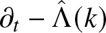 $\partial_t - \hat{\Lambda}(k)$ to (9.1), we arrive at the equation
 \begin{equation}
\partial_t \widehat{Z}_{\mathrm{c}} = \hat{\Lambda} \widehat{Z}_{\mathrm{c}} + \chi Z_3^{\mathrm{res}}\big(\widehat{Z}_{\mathrm{c}},\widehat{Z}_{\mathrm{c}},\widehat{Z}_{\mathrm{c}}\big) + \chi \mathcal{E}_4(\cdot,t).
\end{equation}
\begin{equation}
\partial_t \widehat{Z}_{\mathrm{c}} = \hat{\Lambda} \widehat{Z}_{\mathrm{c}} + \chi Z_3^{\mathrm{res}}\big(\widehat{Z}_{\mathrm{c}},\widehat{Z}_{\mathrm{c}},\widehat{Z}_{\mathrm{c}}\big) + \chi \mathcal{E}_4(\cdot,t).
\end{equation} We bound the critical cubic nonlinearity  $Z_3^{\mathrm{res}}$ in (9.5).
Lemma 9.1. We have
 \begin{equation}
\big\|\partial_k^j Z_3^{\mathrm{res}}\big({\widehat{V}},{\widehat{W}},\widehat{Z}\big)\big\|_{L^\infty} \lesssim \big\|{\widehat{V}}\big\|_{W^{j,1}}\big\|{\widehat{W}}\big\|_{L^\infty}\big\|\widehat{Z}\big\|_{L^1},
\end{equation}
\begin{equation}
\big\|\partial_k^j Z_3^{\mathrm{res}}\big({\widehat{V}},{\widehat{W}},\widehat{Z}\big)\big\|_{L^\infty} \lesssim \big\|{\widehat{V}}\big\|_{W^{j,1}}\big\|{\widehat{W}}\big\|_{L^\infty}\big\|\widehat{Z}\big\|_{L^1},
\end{equation}for  ${\widehat{V}},{\widehat{W}}, \widehat{Z} \in C_c(-k_0,k_0) \cap \mathcal{X}$ and
  $j = 0,1$ (with
  $j = 0$ in case
  $\mathcal{X} = Y_0$).
Proof. Young’s convolution inequality yields
 \begin{align*}
\big\|\partial_k^j B_3\big({\widehat{V}},{\widehat{W}},\widehat{Z}\big)\big\|_{L^\infty} \lesssim \big\|{\widehat{V}}\big\|_{W^{j,1}}\big\|{\widehat{W}}\big\|_{L^\infty}\big\|\widehat{Z}\big\|_{L^1},
\end{align*}
\begin{align*}
\big\|\partial_k^j B_3\big({\widehat{V}},{\widehat{W}},\widehat{Z}\big)\big\|_{L^\infty} \lesssim \big\|{\widehat{V}}\big\|_{W^{j,1}}\big\|{\widehat{W}}\big\|_{L^\infty}\big\|\widehat{Z}\big\|_{L^1},
\end{align*}for  $j = 0,1$ and
 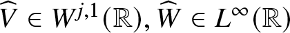 ${\widehat{V}} \in W^{j,1}(\mathbb{R}), {\widehat{W}} \in L^\infty(\mathbb{R})$ and
  $\widehat{Z} \in L^1(\mathbb{R})$. Combining the latter with the estimates on
  $Q_3^1$ and
  $Q_3^2$ established in Proposition 7.1 we infer (9.6).
Next, we obtain a bound on the residual nonlinearity  $\mathcal{E}_4(\cdot,t)$ in (9.5).
Lemma 9.2. There exists a  $t$- and
  $k$-independent constant
  $C \gt 0$ such that, if
  $k \in \mathbb{R}$ and
  $t \in [0,T_{\max})$ with
  $\|\widehat{U}(t)\|_{L^1 \cap L^\infty} \leq 1$, then we have the bound
 \begin{align*}
\left|\partial_k^j\left(\chi(k) \mathcal{E}_4(k,t)\right)\right| &\leq C\left(\big\|\widehat{U}(t)\big\|_{W^{j,1}} \big\|\widehat{U}(t)\big\|_{L^1} \left(\big\|\widehat{U}(t)\big\|_{L^1} + \big\|\widehat{U}_\mathrm{s}(t)\big\|_{L^\infty}\right) \right.\\
&\left.\qquad + \, \big\|\widehat{U}_\mathrm{s}(t)\big\|_{W^{j,1}}\big\|\widehat{U}_\mathrm{s}(t)\big\|_{L^\infty} + |\chi(k) k| \big\|\widehat{U}_\mathrm{s}(t)\big\|_{L^\infty} \big\|\widehat{U}(t)\big\|_{W^{j,1}} \right. \\
&\left.\qquad + \, \big\|\widehat{U}_\mathrm{s}(t)\big\|_{L^\infty} \big\||\cdot|\widehat{U}_\mathrm{c}(t)\big\|_{W^{j,1}} + \big\|\widehat{U}_\mathrm{s}(t)\big\|_{L^1} \big\|\widehat{U}(t)\big\|_{W^{j,1}}\right),
\end{align*}
\begin{align*}
\left|\partial_k^j\left(\chi(k) \mathcal{E}_4(k,t)\right)\right| &\leq C\left(\big\|\widehat{U}(t)\big\|_{W^{j,1}} \big\|\widehat{U}(t)\big\|_{L^1} \left(\big\|\widehat{U}(t)\big\|_{L^1} + \big\|\widehat{U}_\mathrm{s}(t)\big\|_{L^\infty}\right) \right.\\
&\left.\qquad + \, \big\|\widehat{U}_\mathrm{s}(t)\big\|_{W^{j,1}}\big\|\widehat{U}_\mathrm{s}(t)\big\|_{L^\infty} + |\chi(k) k| \big\|\widehat{U}_\mathrm{s}(t)\big\|_{L^\infty} \big\|\widehat{U}(t)\big\|_{W^{j,1}} \right. \\
&\left.\qquad + \, \big\|\widehat{U}_\mathrm{s}(t)\big\|_{L^\infty} \big\||\cdot|\widehat{U}_\mathrm{c}(t)\big\|_{W^{j,1}} + \big\|\widehat{U}_\mathrm{s}(t)\big\|_{L^1} \big\|\widehat{U}(t)\big\|_{W^{j,1}}\right),
\end{align*}for  $j = 0,1$ (with
  $j = 0$ in case
  $\mathcal{X} = Y_0$).
Proof. We recall that  $Z_3^{\mathrm{res}}$ is a trilinear form. So, the result follows by combining Lemma 9.1 with the estimates on
  $\mathcal{E}, Q_2, \mathcal{E}_2, K_3$ and
  $\mathcal{E}_3$ established in Lemma 6.1 and Propositions 7.1 and 8.1.
10. Reduced equations
In this section, we take  $\mathcal{X} = X_0$. Our aim is to capture the leading-order temporal dynamics of
  $\widehat{Z}_{\mathrm{c}}(k,t)$ by proceeding as in [Reference de Rijk and Schneider10, Theorem 1.5] and decomposing
  $\widehat{Z}_{\mathrm{c}}(k,t)$ into an explicit leading-order Gaussian part and a remainder vanishing at the critical frequency
  $k = 0$. In order to control the leading-order Gaussian part, we derive an ordinary differential equation for
  $A(t) \,\smash{\overset{\scriptscriptstyle{\mathrm{def}}}{=} \mathrm{e}^{-\hat{\Lambda}(0)(t+1)} \widehat{Z}_{\mathrm{c}}(0,t)}$. If the sign condition (1.7) is fulfilled, the cubic term in this ODE is of absorption type, which induces enhanced diffusive decay of the Gaussian part. Moreover, we derive an equation for the remainder and obtain estimates on the nonlinearities by exploiting that the remainder vanishes at frequency
  $k = 0$. These findings turn out to be sufficient to close a global nonlinear iteration argument in the next section, yielding the proof of Theorem 1.1.
Thus, we introduce the new variables
 \begin{equation}
A(t) \overset{\scriptscriptstyle{\mathrm{def}}}{=} \mathrm{e}^{-\hat{\Lambda}(0)(t+1)} \widehat{Z}_{\mathrm{c}}(0,t), \qquad \varsigma_{\mathrm{c}}(k,t) \overset{\scriptscriptstyle{\mathrm{def}}}{=} \mathrm{e}^{\hat{\Lambda}(k) (t+1)} \chi(k) A(t),
\end{equation}
\begin{equation}
A(t) \overset{\scriptscriptstyle{\mathrm{def}}}{=} \mathrm{e}^{-\hat{\Lambda}(0)(t+1)} \widehat{Z}_{\mathrm{c}}(0,t), \qquad \varsigma_{\mathrm{c}}(k,t) \overset{\scriptscriptstyle{\mathrm{def}}}{=} \mathrm{e}^{\hat{\Lambda}(k) (t+1)} \chi(k) A(t),
\end{equation}and decompose
 \begin{equation}
\widehat{Z}_{\mathrm{c}}(k,t) = \varsigma_{\mathrm{c}}(k,t) + \widehat{\rho}_{\mathrm{c}}(k,t),
\end{equation}
\begin{equation}
\widehat{Z}_{\mathrm{c}}(k,t) = \varsigma_{\mathrm{c}}(k,t) + \widehat{\rho}_{\mathrm{c}}(k,t),
\end{equation}where the residual
 \begin{align*}
\widehat{\rho}_{\mathrm{c}}(k,t) \overset{\scriptscriptstyle{\mathrm{def}}}{=} \mathrm{e}^{\hat{\Lambda}(k) (t+1)} \chi(k) A(t) - \widehat{Z}_{\mathrm{c}}(k,t),
\end{align*}
\begin{align*}
\widehat{\rho}_{\mathrm{c}}(k,t) \overset{\scriptscriptstyle{\mathrm{def}}}{=} \mathrm{e}^{\hat{\Lambda}(k) (t+1)} \chi(k) A(t) - \widehat{Z}_{\mathrm{c}}(k,t),
\end{align*}vanishes at  $k = 0$ for each
  $t \in [0,T_{\max})$. We note that
  $A(t)$ is real for each
  $t \in [0,T_{\max})$ by (5.5), (9.2) and the fact that
 \begin{equation}
\mathrm{e}^{-\hat{\Lambda}(0) (t+1)} = \begin{pmatrix} \cos(t+1) & -\sin(t+1)\\ \sin(t+1) & \cos(t+1)\end{pmatrix},
\end{equation}
\begin{equation}
\mathrm{e}^{-\hat{\Lambda}(0) (t+1)} = \begin{pmatrix} \cos(t+1) & -\sin(t+1)\\ \sin(t+1) & \cos(t+1)\end{pmatrix},
\end{equation}  $Q_2(\widehat{U}_\mathrm{c}(t),\widehat{U}_\mathrm{c}(t))(0)$ and
  $K_2(\widehat{U}_\mathrm{c}(t),\widehat{U}_\mathrm{c}(t),\widehat{U}_\mathrm{c}(t))(0)$ are real by Propositions 7.1 and 8.1. So, by (9.3), smoothness of
  $\hat{\Lambda}(\cdot)$ and
  $\chi$, and the fact that
  $\chi$ has compact support, we infer
 \begin{equation}
A \in C\big([0,T_{\max}),\mathbb{R}\big), \qquad \widehat{\rho}_{\mathrm{c}},\varsigma_{\mathrm{c}} \in C\big([0,T_{\max}),W^{1,1}(\mathbb{R})\cap W^{1,\infty}(\mathbb{R})\big).
\end{equation}
\begin{equation}
A \in C\big([0,T_{\max}),\mathbb{R}\big), \qquad \widehat{\rho}_{\mathrm{c}},\varsigma_{\mathrm{c}} \in C\big([0,T_{\max}),W^{1,1}(\mathbb{R})\cap W^{1,\infty}(\mathbb{R})\big).
\end{equation} Substituting  $\widehat{Z}_{\mathrm{c}}(k,t) = \mathrm{e}^{\hat{\Lambda}(k) (t+1)} \chi(k) A(t) + \widehat{\rho}_{\mathrm{c}}(k,t)$ into (9.5) we arrive at
 \begin{equation}
\begin{aligned}
\mathrm{e}^{\hat{\Lambda}(k) (t+1)} \chi(k) A'(t) + \partial_t \widehat{\rho}_{\mathrm{c}}(k,t) &= \hat{\Lambda}(k) \widehat{\rho}_{\mathrm{c}}(k,t) + \chi(k) Z_3^{\mathrm{res}}\big(\widehat{Z}_{\mathrm{c}}(t),\widehat{Z}_{\mathrm{c}}(t),\widehat{Z}_{\mathrm{c}}(t)\big)(k)\\ \qquad + \, \chi(k) \mathcal{E}_4(k,t),
\end{aligned}
\end{equation}
\begin{equation}
\begin{aligned}
\mathrm{e}^{\hat{\Lambda}(k) (t+1)} \chi(k) A'(t) + \partial_t \widehat{\rho}_{\mathrm{c}}(k,t) &= \hat{\Lambda}(k) \widehat{\rho}_{\mathrm{c}}(k,t) + \chi(k) Z_3^{\mathrm{res}}\big(\widehat{Z}_{\mathrm{c}}(t),\widehat{Z}_{\mathrm{c}}(t),\widehat{Z}_{\mathrm{c}}(t)\big)(k)\\ \qquad + \, \chi(k) \mathcal{E}_4(k,t),
\end{aligned}
\end{equation}for  $k \in \mathbb{R}$ and
  $t \in [0,T_{\max})$. Setting
  $k = 0$ in (10.5), we find
 \begin{equation}
\mathrm{e}^{\hat{\Lambda}(0) (t+1)} A'(t) = Z_3^{\mathrm{res}}\big(\widehat{Z}_{\mathrm{c}}(t),\widehat{Z}_{\mathrm{c}}(t),\widehat{Z}_{\mathrm{c}}(t)\big)(0) + \mathcal{E}_4(0,t),
\end{equation}
\begin{equation}
\mathrm{e}^{\hat{\Lambda}(0) (t+1)} A'(t) = Z_3^{\mathrm{res}}\big(\widehat{Z}_{\mathrm{c}}(t),\widehat{Z}_{\mathrm{c}}(t),\widehat{Z}_{\mathrm{c}}(t)\big)(0) + \mathcal{E}_4(0,t),
\end{equation}for  $t \in [0,T_{\max})$. Subsequently, inserting (10.6) into (10.5), we obtain
 \begin{equation}
\partial_t \widehat{\rho}_{\mathrm{c}}(k,t) = \hat{\Lambda}(k) \widehat{\rho}_{\mathrm{c}}(k,t) + \chi(k) \left(\mathcal{E}_4(k,t) - \mathrm{e}^{\hat{\Lambda}(k) (t+1)} \mathrm{e}^{-\hat{\Lambda}(0) (t+1)} \mathcal{E}_4(0,t) + \mathcal{E}_5(k,t)\right),
\end{equation}
\begin{equation}
\partial_t \widehat{\rho}_{\mathrm{c}}(k,t) = \hat{\Lambda}(k) \widehat{\rho}_{\mathrm{c}}(k,t) + \chi(k) \left(\mathcal{E}_4(k,t) - \mathrm{e}^{\hat{\Lambda}(k) (t+1)} \mathrm{e}^{-\hat{\Lambda}(0) (t+1)} \mathcal{E}_4(0,t) + \mathcal{E}_5(k,t)\right),
\end{equation}where we denote
 \begin{align*}
\mathcal{E}_5(k,t) &= Z_3^{\mathrm{res}}\big(\widehat{Z}_{\mathrm{c}}(t),\widehat{Z}_{\mathrm{c}}(t),\widehat{Z}_{\mathrm{c}}(t)\big)(k) - \mathrm{e}^{\hat{\Lambda}(k) (t+1)} \mathrm{e}^{-\hat{\Lambda}(0) (t+1)} Z_3^{\mathrm{res}}\big(\widehat{Z}_{\mathrm{c}}(t),\widehat{Z}_{\mathrm{c}}(t),\widehat{Z}_{\mathrm{c}}(t)\big)(0),
\end{align*}
\begin{align*}
\mathcal{E}_5(k,t) &= Z_3^{\mathrm{res}}\big(\widehat{Z}_{\mathrm{c}}(t),\widehat{Z}_{\mathrm{c}}(t),\widehat{Z}_{\mathrm{c}}(t)\big)(k) - \mathrm{e}^{\hat{\Lambda}(k) (t+1)} \mathrm{e}^{-\hat{\Lambda}(0) (t+1)} Z_3^{\mathrm{res}}\big(\widehat{Z}_{\mathrm{c}}(t),\widehat{Z}_{\mathrm{c}}(t),\widehat{Z}_{\mathrm{c}}(t)\big)(0),
\end{align*}for  $t \in [0,T_{\max})$ and
  $k \in \mathbb{R}$.
In our nonlinear argument, we control the dynamics of the residual  $\widehat{\rho}_{\mathrm{c}}(t)$ through iterative estimates on the Duhamel formulation associated with (10.7). The nonlinear term
  $\mathcal{E}_4(\cdot,t)$ in (10.7) can be bounded with the aid of Lemma 9.2. Moreover, the following result provides a bound on the term
  $\mathcal{E}_5(\cdot,t)$ in (10.7).
Lemma 10.1. There exists a  $t$-independent constant
  $C \gt 0$ such that
 \begin{align*}
\left\|\partial_k^j \mathcal{E}_5(\cdot,t)\right\|_{L^\infty} &\leq C \left(\frac{|A(t)|}{\sqrt{1+t}} + \big\|\widehat{\rho}_{\mathrm{c}}(t)\big\|_{L^1}\right) \left(|A(t)| + \big\|\widehat{\rho}_{\mathrm{c}}(t)\big\|_{L^\infty}\right)\\
&\qquad \cdot \left((1+t)^{-\frac12(1-j)} |A(t)| + \big\|\widehat{\rho}_{\mathrm{c}}(t)\big\|_{W^{j,1}} + (1+t)^{\frac{j}{2}} \big\|\widehat{\rho}_{\mathrm{c}}(t)\big\|_{L^1}\right),
\end{align*}
\begin{align*}
\left\|\partial_k^j \mathcal{E}_5(\cdot,t)\right\|_{L^\infty} &\leq C \left(\frac{|A(t)|}{\sqrt{1+t}} + \big\|\widehat{\rho}_{\mathrm{c}}(t)\big\|_{L^1}\right) \left(|A(t)| + \big\|\widehat{\rho}_{\mathrm{c}}(t)\big\|_{L^\infty}\right)\\
&\qquad \cdot \left((1+t)^{-\frac12(1-j)} |A(t)| + \big\|\widehat{\rho}_{\mathrm{c}}(t)\big\|_{W^{j,1}} + (1+t)^{\frac{j}{2}} \big\|\widehat{\rho}_{\mathrm{c}}(t)\big\|_{L^1}\right),
\end{align*}for  $j = 0,1$ and
  $t \in [0,T_{\max})$.
Proof. With the aid of Lemma 4.1, we infer
 \begin{equation}
\left\|\partial_k^j \left(\chi \mathrm{e}^{\hat{\Lambda}(\cdot) (t+1)}\right)\right\|_{L^p} \lesssim \left\|(1 + j|\cdot|(t+1) ) \mathrm{e}^{-\frac12 \alpha |\cdot|^2 (t+1)}\right\|_{L^p} \lesssim (1+t)^{-\frac{1}{2p} + \frac{j}{2}},
\end{equation}
\begin{equation}
\left\|\partial_k^j \left(\chi \mathrm{e}^{\hat{\Lambda}(\cdot) (t+1)}\right)\right\|_{L^p} \lesssim \left\|(1 + j|\cdot|(t+1) ) \mathrm{e}^{-\frac12 \alpha |\cdot|^2 (t+1)}\right\|_{L^p} \lesssim (1+t)^{-\frac{1}{2p} + \frac{j}{2}},
\end{equation}for  $t \geq 0$,
  $p = 1,\infty$ and
  $j = 0,1$. Therefore, we find a
  $t$-independent constant
  $C_1 \gt 0$ such that
 \begin{equation}
\big\|\partial_k^j \widehat{Z}_{\mathrm{c}}(t)\big\|_{L^p} \leq C_1 \left(\big\|\partial_k^j \widehat{\rho}_{\mathrm{c}}(t)\big\|_{L^p} + (1+t)^{-\frac{1}{2p} + \frac{j}{2}} |A(t)| \right),
\end{equation}
\begin{equation}
\big\|\partial_k^j \widehat{Z}_{\mathrm{c}}(t)\big\|_{L^p} \leq C_1 \left(\big\|\partial_k^j \widehat{\rho}_{\mathrm{c}}(t)\big\|_{L^p} + (1+t)^{-\frac{1}{2p} + \frac{j}{2}} |A(t)| \right),
\end{equation}for  $j = 0,1$,
  $p = 1,\infty$ and
  $t \in [0,T_{\max})$. On the other hand, combining (10.8) with identity (10.3) and Lemma 9.1, we obtain a
  $t$-independent constant
 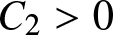 $C_2 \gt 0$ such that
 \begin{align*}
\left\|\partial_k^j \mathcal{E}_5(\cdot,t)\right\|_{L^\infty} &\leq C_2\big\|\widehat{Z}_{\mathrm{c}}(t)\big\|_{L^1} \big\|\widehat{Z}_{\mathrm{c}}(t)\big\|_{L^\infty} \left(\big\|\widehat{Z}_{\mathrm{c}}(t)\big\|_{W^{j,1}} + (1+t)^{\frac{j}2} \big\|\widehat{Z}_{\mathrm{c}}(t)\big\|_{L^1}\right),
\end{align*}
\begin{align*}
\left\|\partial_k^j \mathcal{E}_5(\cdot,t)\right\|_{L^\infty} &\leq C_2\big\|\widehat{Z}_{\mathrm{c}}(t)\big\|_{L^1} \big\|\widehat{Z}_{\mathrm{c}}(t)\big\|_{L^\infty} \left(\big\|\widehat{Z}_{\mathrm{c}}(t)\big\|_{W^{j,1}} + (1+t)^{\frac{j}2} \big\|\widehat{Z}_{\mathrm{c}}(t)\big\|_{L^1}\right),
\end{align*}for  $j = 0,1$ and
  $t \in [0,T_{\max})$, which proves the result by inserting (10.9) into the latter.
The fact that the residual  $\widehat{\rho}_{\mathrm{c}}(k,t)$ vanishes at the critical frequency
  $k = 0$ suggests that
  $\widehat{\rho}_{\mathrm{c}}(k,t)$ decays at a higher rate than
  $A(t)$. Indeed, neglecting the nonlinear terms in the equation (10.7) for
  $\smash{\widehat{\rho}_{\mathrm{c}}(k,t)}$, we find that
  $\smash{\widehat{\rho}_{\mathrm{c}}(k,t) = \mathrm{e}^{\hat{\Lambda}(k) t} \widehat{\rho}_{\mathrm{c}}(k,0) \approx k \mathrm{e}^{\hat{\Lambda}(k) t} \partial_k \widehat{\rho}_{\mathrm{c}}(0,0)}$ decays at rate
  $\smash{t^{-\frac12}}$ in
 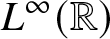 $L^\infty(\mathbb{R})$ and at rate
  $t^{-1}$ in
  $L^1(\mathbb{R})$ by Lemma 4.1. As argued in §9, the nonlinear terms with an
 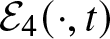 $\mathcal{E}_4(\cdot,t)$-contribution in (10.7) are controllable using standard
  $L^1$-
 $L^\infty$-estimates in combination with the bounds from Lemma 9.2.
Now, let’s look at the remaining nonlinear term
 \begin{equation}
\int_0^t \mathrm{e}^{\hat{\Lambda}(k)(t-s)} \chi(k) \mathcal{E}_5(k,s) \mathrm{d} s,
\end{equation}
\begin{equation}
\int_0^t \mathrm{e}^{\hat{\Lambda}(k)(t-s)} \chi(k) \mathcal{E}_5(k,s) \mathrm{d} s,
\end{equation}arising in the Duhamel formula of  $\widehat{\rho}_{\mathrm{c}}(k,t)$. Applying the mean value theorem and using
 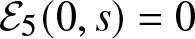 $\mathcal{E}_5(0,s) = 0$, we can bound
 \begin{equation}
\left|\mathcal{E}_5(k,s)\right| \leq |k| \left\|\partial_k \mathcal{E}_5(\cdot,s)\right\|_{L^\infty}.
\end{equation}
\begin{equation}
\left|\mathcal{E}_5(k,s)\right| \leq |k| \left\|\partial_k \mathcal{E}_5(\cdot,s)\right\|_{L^\infty}.
\end{equation} So, we have the choice to bound  $\mathcal{E}_5(k,s)$ in (10.10) using the estimate in Lemma 10.1 with
  $j = 0$ or using (10.11) and the estimate in Lemma 10.1 with
  $j = 1$. By the previous considerations, the terms occurring on the right-hand side of these bounds are all integrable, i.e. decaying at rate
  $(1+s)^{-a}$ with
  $a \gt 1$ and, thus, controllable with standard
  $L^1$-
 $L^\infty$-estimates, except for the marginal terms
 \begin{align*}
\frac{|A(s)|^3}{1+s}, \qquad \frac{|k| |A(s)|^3}{\sqrt{1+s}},
\end{align*}
\begin{align*}
\frac{|A(s)|^3}{1+s}, \qquad \frac{|k| |A(s)|^3}{\sqrt{1+s}},
\end{align*}arising on the right-hand side of the bounds on  $\|\mathcal{E}_5(\cdot,s)\|_{L^\infty}$ and
  $|k| \left\|\partial_k \mathcal{E}_5(\cdot,s)\right\|_{L^\infty}$, respectively, cf. Lemma 10.1. Since we have the freedom to choose between these bounds for each
  $s \in [0,t]$, we can, using Lemma 4.1, estimate the marginal terms in (10.10) in
  $L^1(\mathbb{R})$ as
 \begin{align*}
\int_0^{\frac{t}2} \frac{|A(s)|^3}{(t-s)\sqrt{1+s}} \mathrm{d} s + \int_{\frac{t}2}^t \frac{|A(s)|^3}{\sqrt{t-s}(1+s)} \mathrm{d} s,
\end{align*}
\begin{align*}
\int_0^{\frac{t}2} \frac{|A(s)|^3}{(t-s)\sqrt{1+s}} \mathrm{d} s + \int_{\frac{t}2}^t \frac{|A(s)|^3}{\sqrt{t-s}(1+s)} \mathrm{d} s,
\end{align*}and in  $L^\infty(\mathbb{R})$ as
 \begin{align*}
\int_0^t \frac{|A(s)|^3}{\sqrt{t-s}\sqrt{1+s}} \mathrm{d} s,
\end{align*}
\begin{align*}
\int_0^t \frac{|A(s)|^3}{\sqrt{t-s}\sqrt{1+s}} \mathrm{d} s,
\end{align*}which suffices to close the nonlinear argument, as we will see in the upcoming section.
Next, we shift focus to the ordinary differential equation (10.6) for  $A(t)$. Applying the projections
  $P_\pm(0)$ to (10.6), we arrive at
 \begin{equation}
\partial_t \left(P_\pm(0) A(t)\right) = \mathrm{e}^{\mp \mathrm{i} (t+1)} P_\pm(0) Z_3^{\mathrm{res}}\big(\widehat{Z}_{\mathrm{c}}(t),\widehat{Z}_{\mathrm{c}}(t),\widehat{Z}_{\mathrm{c}}(t)\big)(0) + \mathrm{e}^{\mp \mathrm{i} (t+1)} P_\pm(0) \mathcal{E}_4(0,t),
\end{equation}
\begin{equation}
\partial_t \left(P_\pm(0) A(t)\right) = \mathrm{e}^{\mp \mathrm{i} (t+1)} P_\pm(0) Z_3^{\mathrm{res}}\big(\widehat{Z}_{\mathrm{c}}(t),\widehat{Z}_{\mathrm{c}}(t),\widehat{Z}_{\mathrm{c}}(t)\big)(0) + \mathrm{e}^{\mp \mathrm{i} (t+1)} P_\pm(0) \mathcal{E}_4(0,t),
\end{equation}for  $t \in [0,T_{\max})$. As argued above, the nonlinear term
  $\mathrm{e}^{\mp \mathrm{i} (t+1)} P_\pm(0)\mathcal{E}_4(0,t)$ is irrelevant in the sense that it can be controlled with standard iterative
  $L^1$-
 $L^\infty$-estimates by invoking Lemma 9.2. The following result provides an approximation of the leading-order nonlinear term in (10.12), which follows by expanding
  $Z_3^{\mathrm{res}}(\widehat{Z}_{\mathrm{c}}(t),\widehat{Z}_{\mathrm{c}}(t),\widehat{Z}_{\mathrm{c}}(t))(0)$ using the decomposition (10.2).
Lemma 10.2. There exists a  $t$-independent constant
  $C \gt 0$ such that
 \begin{align*}
\mathcal{E}_6(t) = P_{\pm}(0) Z_3^{\mathrm{res}}\big(\widehat{Z}_{\mathrm{c}}(t),\widehat{Z}_{\mathrm{c}}(t),\widehat{Z}_{\mathrm{c}}(t)\big)(0) - \frac{\omega_\pm \mathrm{e}^{\pm \mathrm{i}(t+1)}}{1+t} \left|\left(P_\pm(0) A(t)\right)_1\right|^2 \left(P_\pm(0) A(t)\right)_1 \begin{pmatrix} 1 \\ \mathrm{i}\end{pmatrix},
\end{align*}
\begin{align*}
\mathcal{E}_6(t) = P_{\pm}(0) Z_3^{\mathrm{res}}\big(\widehat{Z}_{\mathrm{c}}(t),\widehat{Z}_{\mathrm{c}}(t),\widehat{Z}_{\mathrm{c}}(t)\big)(0) - \frac{\omega_\pm \mathrm{e}^{\pm \mathrm{i}(t+1)}}{1+t} \left|\left(P_\pm(0) A(t)\right)_1\right|^2 \left(P_\pm(0) A(t)\right)_1 \begin{pmatrix} 1 \\ \mathrm{i}\end{pmatrix},
\end{align*}can be bounded by
 \begin{align*}
\left|\mathcal{E}_6(t)\right| \leq C \left(\big\|\widehat{\rho}_{\mathrm{c}}(t)\big\|_{L^\infty}\left( \big\|\widehat{\rho}_{\mathrm{c}}(t)\big\|_{L^1} + \frac{|A(t)|}{\sqrt{1+t}} \right)^2 + \frac{|A(t)|^3}{(1+t)^{\frac32}} \right),
\end{align*}
\begin{align*}
\left|\mathcal{E}_6(t)\right| \leq C \left(\big\|\widehat{\rho}_{\mathrm{c}}(t)\big\|_{L^\infty}\left( \big\|\widehat{\rho}_{\mathrm{c}}(t)\big\|_{L^1} + \frac{|A(t)|}{\sqrt{1+t}} \right)^2 + \frac{|A(t)|^3}{(1+t)^{\frac32}} \right),
\end{align*}for  $t \in [0,T_{\max})$, where the coefficients
  $\omega_\pm \in \mathbb{C}$ are given by
 \begin{align*}
\omega_\pm = \frac{\mp \pi \mathrm{i} \left(9\beta + 10\kappa^2\right)}{3 \sqrt{3\alpha^2 + 1 \mp 2 \mathrm{i} \alpha}}.
\end{align*}
\begin{align*}
\omega_\pm = \frac{\mp \pi \mathrm{i} \left(9\beta + 10\kappa^2\right)}{3 \sqrt{3\alpha^2 + 1 \mp 2 \mathrm{i} \alpha}}.
\end{align*}Proof. Firstly, we note that by Lemma 4.1, there exists a  $t$-independent constant
  $C_1 \gt 0$ such that
 \begin{equation}
\|\varsigma_{\mathrm{c}}(t)\|_{L^1} \leq |A(t)| \left\|\mathrm{e}^{\hat{\Lambda}(\cdot) (t+1)}\right\|_{L^1} \leq C_1 \frac{|A(t)|}{\sqrt{1+t}},
\end{equation}
\begin{equation}
\|\varsigma_{\mathrm{c}}(t)\|_{L^1} \leq |A(t)| \left\|\mathrm{e}^{\hat{\Lambda}(\cdot) (t+1)}\right\|_{L^1} \leq C_1 \frac{|A(t)|}{\sqrt{1+t}},
\end{equation}for  $t \in [0,T_{\max})$. Next, we expand
 \begin{align*}
\chi(k) Z_3^{\mathrm{res}}(\widehat{Z}_{\mathrm{c}}(t),\widehat{Z}_{\mathrm{c}}(t),\widehat{Z}_{\mathrm{c}}(t))(k) &= \chi(k) Z_3^{\mathrm{res}}\big(\varsigma_{\mathrm{c}}(t),\varsigma_{\mathrm{c}}(t),\varsigma_{\mathrm{c}}(t)\big)(k) + E_1(k,t),
\end{align*}
\begin{align*}
\chi(k) Z_3^{\mathrm{res}}(\widehat{Z}_{\mathrm{c}}(t),\widehat{Z}_{\mathrm{c}}(t),\widehat{Z}_{\mathrm{c}}(t))(k) &= \chi(k) Z_3^{\mathrm{res}}\big(\varsigma_{\mathrm{c}}(t),\varsigma_{\mathrm{c}}(t),\varsigma_{\mathrm{c}}(t)\big)(k) + E_1(k,t),
\end{align*}with remainder
 \begin{align*}
E_1(k,t) = \chi(k) \left(Z_3^{\mathrm{res}}\big(\widehat{Z}_{\mathrm{c}}(t),\widehat{Z}_{\mathrm{c}}(t),\widehat{Z}_{\mathrm{c}}(t)\big)(k) - Z_3^{\mathrm{res}}\big(\varsigma_{\mathrm{c}}(t),\varsigma_{\mathrm{c}}(t),\varsigma_{\mathrm{c}}(t)\big)(k)\right),
\end{align*}
\begin{align*}
E_1(k,t) = \chi(k) \left(Z_3^{\mathrm{res}}\big(\widehat{Z}_{\mathrm{c}}(t),\widehat{Z}_{\mathrm{c}}(t),\widehat{Z}_{\mathrm{c}}(t)\big)(k) - Z_3^{\mathrm{res}}\big(\varsigma_{\mathrm{c}}(t),\varsigma_{\mathrm{c}}(t),\varsigma_{\mathrm{c}}(t)\big)(k)\right),
\end{align*}for  $k \in \mathbb{R}$ and
  $t \in [0,T_{\max})$. The fact that
  $Z^3_{\mathrm{res}}$ is trilinear in combination with Lemma 9.1, identity (10.2) and estimate (10.13) yield
  $t$-independent constants
 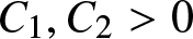 $C_1,C_2 \gt 0$ such that
 \begin{equation}
\begin{aligned}
\left\|E_1(\cdot,t)\right\|_{L^\infty} &\leq C_1\big\|\widehat{\rho}_{\mathrm{c}}(t)\big\|_{L^\infty}\left( \big\|\widehat{\rho}_{\mathrm{c}}(t)\big\|_{L^1} + \big\|\varsigma_{\mathrm{c}}(t)\big\|_{L^1} \right)^2\\
&\leq C_2 \big\|\widehat{\rho}_{\mathrm{c}}(t)\big\|_{L^\infty}\left( \big\|\widehat{\rho}_{\mathrm{c}}(t)\big\|_{L^1} + \frac{|A(t)|}{\sqrt{1+t}} \right)^2,
\end{aligned}
\end{equation}
\begin{equation}
\begin{aligned}
\left\|E_1(\cdot,t)\right\|_{L^\infty} &\leq C_1\big\|\widehat{\rho}_{\mathrm{c}}(t)\big\|_{L^\infty}\left( \big\|\widehat{\rho}_{\mathrm{c}}(t)\big\|_{L^1} + \big\|\varsigma_{\mathrm{c}}(t)\big\|_{L^1} \right)^2\\
&\leq C_2 \big\|\widehat{\rho}_{\mathrm{c}}(t)\big\|_{L^\infty}\left( \big\|\widehat{\rho}_{\mathrm{c}}(t)\big\|_{L^1} + \frac{|A(t)|}{\sqrt{1+t}} \right)^2,
\end{aligned}
\end{equation}for  $t \in [0,T_{\max})$.
The expansion (4.2) yields
 \begin{equation}
\left|\lambda_\pm(k) - \tilde{\lambda}_\pm(k)\right| \lesssim |k|^4,
\end{equation}
\begin{equation}
\left|\lambda_\pm(k) - \tilde{\lambda}_\pm(k)\right| \lesssim |k|^4,
\end{equation}for 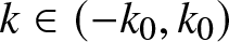 $k \in (-k_0,k_0)$, where
  $\tilde{\lambda}_\pm(k)$ are the quadratic approximants of the eigenvalues
  $\lambda_\pm(k)$, given by (1.21). Clearly, it holds
 \begin{equation}
\operatorname{Re}(\tilde{\lambda}_\pm(k)) \leq -\frac14\alpha\left(k_0^2 + k^2\right),
\end{equation}
\begin{equation}
\operatorname{Re}(\tilde{\lambda}_\pm(k)) \leq -\frac14\alpha\left(k_0^2 + k^2\right),
\end{equation}for  $k \in \mathbb{R} \setminus (-k_0,k_0)$. Moreover, the mean value theorem implies
 \begin{equation}
\left|\mathrm{e}^z - 1\right| \leq \mathrm{e}^{|z|} - 1 \leq |z| \mathrm{e}^{|z|},
\end{equation}
\begin{equation}
\left|\mathrm{e}^z - 1\right| \leq \mathrm{e}^{|z|} - 1 \leq |z| \mathrm{e}^{|z|},
\end{equation}for  $z \in \mathbb{C}$. Thus, combining estimates (10.15), (10.16), (10.17) and taking
  $k_0 \gt 0$ smaller if necessary, we find
  $t$- and
  $k$-independent constants
  $C_{1,2} \gt 0$ such that
 \begin{align*}
&\left|P_{\pm}(k) \varsigma_{\mathrm{c}}(k,t) - P_{\pm}(0) \mathrm{e}^{\tilde{\lambda}_\pm(k) (t+1)} A(t)\right|\\
&\quad \ \leq \left(\left|P_\pm(k)\chi(k)\right| \left|\mathrm{e}^{(\lambda_\pm(k) - \tilde{\lambda}_\pm(k))(t+1)} - 1 \right| + \left|P_\pm(k)\chi(k) - P_\pm(0)\right|\right) \mathrm{e}^{\operatorname{Re}(\tilde{\lambda}_\pm(k)) (t+1)} |A(t)| \\
&\quad \ \leq C_1\left(|k|^4 (t+1) + |k|\right) \mathrm{e}^{-\frac38 \alpha k^2 (t+1)} |A(t)| \leq C_2 |k| \mathrm{e}^{-\frac14 \alpha k^2 (t+1)} |A(t)|,
\end{align*}
\begin{align*}
&\left|P_{\pm}(k) \varsigma_{\mathrm{c}}(k,t) - P_{\pm}(0) \mathrm{e}^{\tilde{\lambda}_\pm(k) (t+1)} A(t)\right|\\
&\quad \ \leq \left(\left|P_\pm(k)\chi(k)\right| \left|\mathrm{e}^{(\lambda_\pm(k) - \tilde{\lambda}_\pm(k))(t+1)} - 1 \right| + \left|P_\pm(k)\chi(k) - P_\pm(0)\right|\right) \mathrm{e}^{\operatorname{Re}(\tilde{\lambda}_\pm(k)) (t+1)} |A(t)| \\
&\quad \ \leq C_1\left(|k|^4 (t+1) + |k|\right) \mathrm{e}^{-\frac38 \alpha k^2 (t+1)} |A(t)| \leq C_2 |k| \mathrm{e}^{-\frac14 \alpha k^2 (t+1)} |A(t)|,
\end{align*}for  $k \in (-k_0,k_0)$ and
  $t \in [0,T_{\max})$, and
 \begin{align*}
\left|P_{\pm}(k) \varsigma_{\mathrm{c}}(k,t) - P_{\pm}(0) \mathrm{e}^{\tilde{\lambda}_\pm(k) (t+1)} A(t)\right| &= \left|P_{\pm}(0) \mathrm{e}^{\tilde{\lambda}_\pm(k) (t+1)} A(t)\right|\\ &\leq C_1 \mathrm{e}^{-\frac14 \alpha k^2(t+1)} \mathrm{e}^{-\frac14 \alpha k_0^2(t+1)} |A(t)|,
\end{align*}
\begin{align*}
\left|P_{\pm}(k) \varsigma_{\mathrm{c}}(k,t) - P_{\pm}(0) \mathrm{e}^{\tilde{\lambda}_\pm(k) (t+1)} A(t)\right| &= \left|P_{\pm}(0) \mathrm{e}^{\tilde{\lambda}_\pm(k) (t+1)} A(t)\right|\\ &\leq C_1 \mathrm{e}^{-\frac14 \alpha k^2(t+1)} \mathrm{e}^{-\frac14 \alpha k_0^2(t+1)} |A(t)|,
\end{align*}for  $k \in \mathbb{R} \setminus (-k_0,k_0)$ and
  $t \in [0,T_{\max})$. Therefore, we obtain a
  $t$-independent constant
  $C \gt 0$ such that
 \begin{equation}
\begin{aligned}
\left\|P_{\pm} \varsigma_{\mathrm{c}}(t) - P_{\pm}(0) \mathrm{e}^{\tilde{\lambda}_\pm(\cdot) (t+1)} A(t)\right\|_{L^p} &\leq \frac{C}{(1+t)^{\frac{1}{2} + \frac{1}{2p}}} |A(t)|, \\
\left\|P_\pm(0) \mathrm{e}^{\tilde{\lambda}_\pm(\cdot) (t+1)} A(t)\right\|_{L^p} &\leq \frac{C}{(1+t)^{\frac{1}{2p}}} |A(t)|,
\end{aligned}
\end{equation}
\begin{equation}
\begin{aligned}
\left\|P_{\pm} \varsigma_{\mathrm{c}}(t) - P_{\pm}(0) \mathrm{e}^{\tilde{\lambda}_\pm(\cdot) (t+1)} A(t)\right\|_{L^p} &\leq \frac{C}{(1+t)^{\frac{1}{2} + \frac{1}{2p}}} |A(t)|, \\
\left\|P_\pm(0) \mathrm{e}^{\tilde{\lambda}_\pm(\cdot) (t+1)} A(t)\right\|_{L^p} &\leq \frac{C}{(1+t)^{\frac{1}{2p}}} |A(t)|,
\end{aligned}
\end{equation}for  $t \in [0,T_{\max})$ and
  $p = 1,\infty$.
Recalling (8.5) and (8.6), we further expand
 \begin{align*}
&Z_3^{\mathrm{res}}\big({\widehat{V}},{\widehat{W}},\widehat{Z}\big)(k)\\
&\quad \ = \sum_{j \in \mathcal{T}} P_{j_0}(k) Z_3\big(P_{j_1} {\widehat{V}}, P_{j_2} {\widehat{W}}, P_{j_3} \widehat{Z}\big)(k) \\
&\quad \ = \sum_{j \in \mathcal{T}} P_{j_0}(k) \int_\mathbb{R} \int_\mathbb{R} \widetilde{N}_3(k,l_1,l_2)\big(P_{j_1} {\widehat{V}}, P_{j_2} {\widehat{W}}, P_{j_3} \widehat{Z}\big) \mathrm{d} l_1 \mathrm{d} l_2\\
&\quad \ = \sum_{j \in \mathcal{T}} \int_\mathbb{R} \int_\mathbb{R} \left[P_{j_0}(k)N_3(k,l_1,l_2)\big(P_{j_1} {\widehat{V}}, P_{j_2} {\widehat{W}}, P_{j_3} \widehat{Z}\big) \phantom{\sum_{m \in \{\pm 1\}} \frac{P_{j_0}(k)}{\phi^2_{(j_0,m,j_3)}}} \right.\\
&\qquad \ \quad + \sum_{m \in \{\pm 1\}} \frac{P_{j_0}(k)}{\phi^2_{(j_0,m,j_3)}(k,l_2)} N_2(k,l_2)\big(\chi P_m N_2(\cdot,l_1-l_2) \big(P_{j_1} {\widehat{V}}, P_{j_2} {\widehat{W}} \big), P_{j_3} \widehat{Z} \big) \\
&\left. \quad \qquad\ + \sum_{m \in \{\pm 1\}} \frac{P_{j_0}(k)}{\phi^2_{(j_0,j_1,m)}(k,l_1)} N_2(k,l_1)\big(P_{j_1} {\widehat{V}} , \chi P_{m} N_2(\cdot,l_2)\big(P_{j_2} {\widehat{W}}, P_{j_3} \widehat{Z}\big)\big) \right] \mathrm{d} l_1 \mathrm{d} l_2,
\end{align*}
\begin{align*}
&Z_3^{\mathrm{res}}\big({\widehat{V}},{\widehat{W}},\widehat{Z}\big)(k)\\
&\quad \ = \sum_{j \in \mathcal{T}} P_{j_0}(k) Z_3\big(P_{j_1} {\widehat{V}}, P_{j_2} {\widehat{W}}, P_{j_3} \widehat{Z}\big)(k) \\
&\quad \ = \sum_{j \in \mathcal{T}} P_{j_0}(k) \int_\mathbb{R} \int_\mathbb{R} \widetilde{N}_3(k,l_1,l_2)\big(P_{j_1} {\widehat{V}}, P_{j_2} {\widehat{W}}, P_{j_3} \widehat{Z}\big) \mathrm{d} l_1 \mathrm{d} l_2\\
&\quad \ = \sum_{j \in \mathcal{T}} \int_\mathbb{R} \int_\mathbb{R} \left[P_{j_0}(k)N_3(k,l_1,l_2)\big(P_{j_1} {\widehat{V}}, P_{j_2} {\widehat{W}}, P_{j_3} \widehat{Z}\big) \phantom{\sum_{m \in \{\pm 1\}} \frac{P_{j_0}(k)}{\phi^2_{(j_0,m,j_3)}}} \right.\\
&\qquad \ \quad + \sum_{m \in \{\pm 1\}} \frac{P_{j_0}(k)}{\phi^2_{(j_0,m,j_3)}(k,l_2)} N_2(k,l_2)\big(\chi P_m N_2(\cdot,l_1-l_2) \big(P_{j_1} {\widehat{V}}, P_{j_2} {\widehat{W}} \big), P_{j_3} \widehat{Z} \big) \\
&\left. \quad \qquad\ + \sum_{m \in \{\pm 1\}} \frac{P_{j_0}(k)}{\phi^2_{(j_0,j_1,m)}(k,l_1)} N_2(k,l_1)\big(P_{j_1} {\widehat{V}} , \chi P_{m} N_2(\cdot,l_2)\big(P_{j_2} {\widehat{W}}, P_{j_3} \widehat{Z}\big)\big) \right] \mathrm{d} l_1 \mathrm{d} l_2,
\end{align*}for  ${\widehat{V}},{\widehat{W}},\widehat{Z} \in C_c(-k_0,k_0) \cap X_0$. So, we readily observe that there exist smooth functions
  $\mathcal{K}_j \colon (-k_0,k_0)^2 \to \mathbb{C}^2$ such that
 \begin{align*}
Z_3^{\mathrm{res}}\big({\widehat{V}},{\widehat{W}},\widehat{Z}\big)(0) &= \sum_{j \in \mathcal{T}} \int_\mathbb{R} \int_\mathbb{R} \mathcal{K}_j(l_1,l_2) \left(P_{j_1}(-l_1) {\widehat{V}}(-l_1)\right)_1 \left(P_{j_2}(l_1-l_2) {\widehat{W}}(l_1-l_2)\right)_1\\ &\qquad \cdot \left(P_{j_3}(l_2) \widehat{Z}(l_2)\right)_1 \mathrm{d} l_1 \mathrm{d} l_2,
\end{align*}
\begin{align*}
Z_3^{\mathrm{res}}\big({\widehat{V}},{\widehat{W}},\widehat{Z}\big)(0) &= \sum_{j \in \mathcal{T}} \int_\mathbb{R} \int_\mathbb{R} \mathcal{K}_j(l_1,l_2) \left(P_{j_1}(-l_1) {\widehat{V}}(-l_1)\right)_1 \left(P_{j_2}(l_1-l_2) {\widehat{W}}(l_1-l_2)\right)_1\\ &\qquad \cdot \left(P_{j_3}(l_2) \widehat{Z}(l_2)\right)_1 \mathrm{d} l_1 \mathrm{d} l_2,
\end{align*}for  ${\widehat{V}},{\widehat{W}},\widehat{Z} \in C_c(-k_0,k_0) \cap X_0$ and
  $j \in \mathcal{T}$. With the aid of (4.4) we compute
 \begin{align*}
\mathcal{K}_j(0,0) &= \left(\beta + \sum_{m \in \{\pm 1\}} \frac{\kappa^2 (P_m(0) \mathbf{e}_2)_1}{\phi^2_{j_0,m,j_3}(0,0)} +
\sum_{m \in \{\pm 1\}} \frac{\kappa^2 (P_m(0) \mathbf{e}_2)_1}{\phi^2_{j_0,j_1,m}(0,0)}\right)P_{j_0}(0)\mathbf{e}_2\\
&= \left(\beta + \sum_{m \in \{\pm 1\}} \frac{\kappa^2 m}{2\left(m + j_3 - j_0\right)} + \sum_{m \in \{\pm 1\}} \frac{\kappa^2 m}{2\left(m + j_1 - j_0\right)}\right)P_{j_0}(0)\mathbf{e}_2,
\end{align*}
\begin{align*}
\mathcal{K}_j(0,0) &= \left(\beta + \sum_{m \in \{\pm 1\}} \frac{\kappa^2 (P_m(0) \mathbf{e}_2)_1}{\phi^2_{j_0,m,j_3}(0,0)} +
\sum_{m \in \{\pm 1\}} \frac{\kappa^2 (P_m(0) \mathbf{e}_2)_1}{\phi^2_{j_0,j_1,m}(0,0)}\right)P_{j_0}(0)\mathbf{e}_2\\
&= \left(\beta + \sum_{m \in \{\pm 1\}} \frac{\kappa^2 m}{2\left(m + j_3 - j_0\right)} + \sum_{m \in \{\pm 1\}} \frac{\kappa^2 m}{2\left(m + j_1 - j_0\right)}\right)P_{j_0}(0)\mathbf{e}_2,
\end{align*}for  $j \in \mathcal{T}$, which implies
 \begin{equation}
P_\pm(0) \sum_{j \in \mathcal{T}} \mathcal{K}_j(0,0) = \left(3\beta + \frac{10}{3} \kappa^2\right) P_\pm(0) \mathbf{e}_2.
\end{equation}
\begin{equation}
P_\pm(0) \sum_{j \in \mathcal{T}} \mathcal{K}_j(0,0) = \left(3\beta + \frac{10}{3} \kappa^2\right) P_\pm(0) \mathbf{e}_2.
\end{equation} In addition, by the smoothness of  $\mathcal{K}_j$, we have
 \begin{align*}
\left|\mathcal{K}_j(l_1,l_2) - \mathcal{K}_j(0,0)\right| \lesssim |l_1| + |l_2|,
\end{align*}
\begin{align*}
\left|\mathcal{K}_j(l_1,l_2) - \mathcal{K}_j(0,0)\right| \lesssim |l_1| + |l_2|,
\end{align*}for  $l_1,l_2 \in (-k_0,k_0)$ and
  $j \in \mathcal{T}$. Thus, combining the latter with Lemma 4.1, (10.13) and (10.18) and setting
 \begin{align*}
\mathcal{Z}(t) &= \sum_{j \in \mathcal{T}} \int_\mathbb{R} \int_\mathbb{R} \mathcal{K}_j(0,0) \left(P_{j_1}(0) \mathrm{e}^{\tilde{\lambda}_{j_1}(l_1)(t+1)} A(t) \right)_1 \left(P_{j_2}(0) \mathrm{e}^{\tilde{\lambda}_{j_2}(l_1-l_2)(t+1)} A(t) \right)_1 \\ &\qquad \cdot \left(P_{j_3}(0) \mathrm{e}^{\tilde{\lambda}_{j_3}(l_2)(t+1)} A(t) \right)_1 \mathrm{d} l_1 \mathrm{d} l_2,
\end{align*}
\begin{align*}
\mathcal{Z}(t) &= \sum_{j \in \mathcal{T}} \int_\mathbb{R} \int_\mathbb{R} \mathcal{K}_j(0,0) \left(P_{j_1}(0) \mathrm{e}^{\tilde{\lambda}_{j_1}(l_1)(t+1)} A(t) \right)_1 \left(P_{j_2}(0) \mathrm{e}^{\tilde{\lambda}_{j_2}(l_1-l_2)(t+1)} A(t) \right)_1 \\ &\qquad \cdot \left(P_{j_3}(0) \mathrm{e}^{\tilde{\lambda}_{j_3}(l_2)(t+1)} A(t) \right)_1 \mathrm{d} l_1 \mathrm{d} l_2,
\end{align*}we obtain  $t$-independent constants
  $C_{1,2} \gt 0$ such that
 \begin{equation}
\begin{aligned}
&\left|Z_3^{\mathrm{res}}\big(\varsigma_{\mathrm{c}}(t),\varsigma_{\mathrm{c}}(t),\varsigma_{\mathrm{c}}(t)\big)(0) - \mathcal{Z}(t)\right|\\
&\quad \ \leq C_1 \left(\int_\mathbb{R} \int_\mathbb{R} \left(|l_1| + |l_2|\right) \left|\mathrm{e}^{\hat{\Lambda}(l_1)(t+1)}\right|\left|\mathrm{e}^{\hat{\Lambda}(l_1-l_2)(t+1)}\right|\left|\mathrm{e}^{\hat{\Lambda}(l_2)(t+1)}\right| |A(t)|^3 \mathrm{d} l_1 \mathrm{d} l_2\right.\\
&\quad \ \qquad \left.+ \, \frac{1}{(1+t)^{\frac32}} |A(t)|^3\right) \\
&\quad \ \leq \frac{C_2}{(1+t)^{\frac{3}{2}}} |A(t)|^3,
\end{aligned}
\end{equation}
\begin{equation}
\begin{aligned}
&\left|Z_3^{\mathrm{res}}\big(\varsigma_{\mathrm{c}}(t),\varsigma_{\mathrm{c}}(t),\varsigma_{\mathrm{c}}(t)\big)(0) - \mathcal{Z}(t)\right|\\
&\quad \ \leq C_1 \left(\int_\mathbb{R} \int_\mathbb{R} \left(|l_1| + |l_2|\right) \left|\mathrm{e}^{\hat{\Lambda}(l_1)(t+1)}\right|\left|\mathrm{e}^{\hat{\Lambda}(l_1-l_2)(t+1)}\right|\left|\mathrm{e}^{\hat{\Lambda}(l_2)(t+1)}\right| |A(t)|^3 \mathrm{d} l_1 \mathrm{d} l_2\right.\\
&\quad \ \qquad \left.+ \, \frac{1}{(1+t)^{\frac32}} |A(t)|^3\right) \\
&\quad \ \leq \frac{C_2}{(1+t)^{\frac{3}{2}}} |A(t)|^3,
\end{aligned}
\end{equation}for  $t \in [0,T_{\max})$. Using the standard integral
 \begin{equation}
\int_\mathbb{R} \mathrm{e}^{-a^2 z^2 + bz} \mathrm{d} z = \frac{\sqrt{\pi}}{a}\mathrm{e}^{\frac{b^2}{4a^2}},
\end{equation}
\begin{equation}
\int_\mathbb{R} \mathrm{e}^{-a^2 z^2 + bz} \mathrm{d} z = \frac{\sqrt{\pi}}{a}\mathrm{e}^{\frac{b^2}{4a^2}},
\end{equation}for  $a, b \in \mathbb{C}$ with
  $\operatorname{Re}(a^2) \gt 0$, cf. [Reference Gradshteyn and Ryzhik19, Integral 3.323.2], and recalling
  $j_0 - j_1 - j_2 - j_3 = 0$, we compute
 \begin{equation}
\begin{aligned}
&\int_\mathbb{R} \int_\mathbb{R} \mathrm{e}^{\left(\tilde{\lambda}_{j_1}(l_1) + \tilde{\lambda}_{j_2}(l_1-l_2) + \tilde{\lambda}_{j_3}(l_2)\right)(t+1)} \mathrm{d} l_1 \mathrm{d} l_2\\
&\quad \ = \frac{2 \pi \mathrm{e}^{(j_1+j_2+j_3) \mathrm{i} (t+1)}}{(t+1)\sqrt{3 \alpha^2 - j_1 j_2 - j_1 j_3 - j_2 j_3 - 2 \mathrm{i} \alpha \left(j_1 + j_2 + j_3\right) }}\\
&\quad \ = \frac{2\pi \mathrm{e}^{j_0 \mathrm{i} (t+1)}}{(t+1)\sqrt{3\alpha^2 + 1 - 2 \mathrm{i} \alpha j_0}},
\end{aligned}
\end{equation}
\begin{equation}
\begin{aligned}
&\int_\mathbb{R} \int_\mathbb{R} \mathrm{e}^{\left(\tilde{\lambda}_{j_1}(l_1) + \tilde{\lambda}_{j_2}(l_1-l_2) + \tilde{\lambda}_{j_3}(l_2)\right)(t+1)} \mathrm{d} l_1 \mathrm{d} l_2\\
&\quad \ = \frac{2 \pi \mathrm{e}^{(j_1+j_2+j_3) \mathrm{i} (t+1)}}{(t+1)\sqrt{3 \alpha^2 - j_1 j_2 - j_1 j_3 - j_2 j_3 - 2 \mathrm{i} \alpha \left(j_1 + j_2 + j_3\right) }}\\
&\quad \ = \frac{2\pi \mathrm{e}^{j_0 \mathrm{i} (t+1)}}{(t+1)\sqrt{3\alpha^2 + 1 - 2 \mathrm{i} \alpha j_0}},
\end{aligned}
\end{equation}for  $j \in \mathcal{T}$ and
  $t \geq 0$. Thus, invoking (4.3), (10.19) and (10.22), we calculate
 \begin{equation}
P_\pm(0) \mathcal{Z}(t) = \frac{2\pi\left(9\beta + 10 \kappa^2\right)\mathrm{e}^{\pm \mathrm{i}(t+1)}}{3(t+1) \sqrt{3\alpha^2 + 1 \mp 2 \mathrm{i} \alpha}} \left|\left(P_{\pm}(0) A(t)\right)_1\right|^2 \left(P_{\pm}(0) A(t)\right)_1 P_{\pm}(0) \mathbf{e}_2,
\end{equation}
\begin{equation}
P_\pm(0) \mathcal{Z}(t) = \frac{2\pi\left(9\beta + 10 \kappa^2\right)\mathrm{e}^{\pm \mathrm{i}(t+1)}}{3(t+1) \sqrt{3\alpha^2 + 1 \mp 2 \mathrm{i} \alpha}} \left|\left(P_{\pm}(0) A(t)\right)_1\right|^2 \left(P_{\pm}(0) A(t)\right)_1 P_{\pm}(0) \mathbf{e}_2,
\end{equation}for  $t \in [0,T_{\max})$. The desired estimate now follows from (4.4), (10.14), (10.20) and (10.23), which concludes the proof.
Since  $A(t)$ is real, we have
  $|(P_\pm(0)A(t))_1| = \frac12 |A(t)|$ by (4.4). Hence, to control the norm of
  $A(t)$, it suffices to control the norm of the first coordinate of
  $P_\pm(0)A(t)$. We express the first coordinate of
  $P_\pm(0)A(t)$ in polar coordinates by setting
 \begin{equation}
(P_\pm(0) A(t))_1 \overset{\scriptscriptstyle{\mathrm{def}}}{=} r_\pm(t) \mathrm{e}^{\mathrm{i} \psi_\pm(t)}.
\end{equation}
\begin{equation}
(P_\pm(0) A(t))_1 \overset{\scriptscriptstyle{\mathrm{def}}}{=} r_\pm(t) \mathrm{e}^{\mathrm{i} \psi_\pm(t)}.
\end{equation} Inserting this into the first component of (10.12), multiplying with  $\smash{\mathrm{e}^{-\mathrm{i}\psi_\pm(t)}}$ and taking real and imaginary parts, we arrive at the real system
 \begin{equation}
r_\pm'(t) = \frac{\operatorname{Re}(\omega_\pm)}{1+t} r_\pm(t)^3 + \operatorname{Re}\left(\mathrm{e}^{-\mathrm{i} \psi_\pm(t) \mp \mathrm{i} (t+1)}\left(P_\pm(0) \mathcal{E}_4(0,t) + \mathcal{E}_6(t)\right)_1\right),
\end{equation}
\begin{equation}
r_\pm'(t) = \frac{\operatorname{Re}(\omega_\pm)}{1+t} r_\pm(t)^3 + \operatorname{Re}\left(\mathrm{e}^{-\mathrm{i} \psi_\pm(t) \mp \mathrm{i} (t+1)}\left(P_\pm(0) \mathcal{E}_4(0,t) + \mathcal{E}_6(t)\right)_1\right),
\end{equation} \begin{equation}
r_\pm(t) \psi_\pm'(t) = \frac{\operatorname{Im}(\omega_\pm)}{1+t} r_\pm(t)^3 + \operatorname{Im}\left(\mathrm{e}^{-\mathrm{i} \psi_\pm(t) \mp \mathrm{i} (t+1)}\left(P_\pm(0) \mathcal{E}_4(0,t) + \mathcal{E}_6(t)\right)_1\right).
\end{equation}
\begin{equation}
r_\pm(t) \psi_\pm'(t) = \frac{\operatorname{Im}(\omega_\pm)}{1+t} r_\pm(t)^3 + \operatorname{Im}\left(\mathrm{e}^{-\mathrm{i} \psi_\pm(t) \mp \mathrm{i} (t+1)}\left(P_\pm(0) \mathcal{E}_4(0,t) + \mathcal{E}_6(t)\right)_1\right).
\end{equation} As mentioned before, we expect that  $\widehat{\rho}_{\mathrm{c}}(k,t)$ exhibits higher-order decay since it vanishes at the critical frequency
  $k = 0$. In fact, we find that the bound on
  $\mathcal{E}_6(t)$, established in Lemma 10.2, is integrable in
  $t$, which implies that, like
  $\mathcal{E}_4(t)$, the residual term
  $\mathcal{E}_6(t)$ can be controlled using standard
  $L^1$-
 $L^\infty$-estimates in our nonlinear argument.
Thus, the critical contributions in (10.25)–(10.26) are the cubic  $r_\pm(t)^3$-terms that cannot be controlled through standard
  $L^1$-
 $L^\infty$-estimates. Here, the sign of
  $\operatorname{Re}(\omega_\pm)$ turns out to be important, as we now see by solving the simpler leading-order system
 \begin{equation}
\begin{aligned}
r_\pm'(t) &= \frac{\operatorname{Re}(\omega_\pm)}{1+t} r_\pm(t)^3,\\
\psi_\pm'(t) &= \frac{\operatorname{Im}(\omega_\pm)}{1+t} r_\pm(t)^2,
\end{aligned}
\end{equation}
\begin{equation}
\begin{aligned}
r_\pm'(t) &= \frac{\operatorname{Re}(\omega_\pm)}{1+t} r_\pm(t)^3,\\
\psi_\pm'(t) &= \frac{\operatorname{Im}(\omega_\pm)}{1+t} r_\pm(t)^2,
\end{aligned}
\end{equation}which is the polar-coordinate representation of the complex ODE (1.6). By separation of variables, it possesses the solution
 \begin{equation}
\begin{aligned}
\tilde{r}_\pm(t) &= \frac{r_\pm(0)}{\sqrt{1-2\operatorname{Re}(\omega_\pm) r_\pm(0)^2 \log(1+t)}},\\
\tilde{\psi}_\pm(t) &= \psi_\pm(0) - \frac{\operatorname{Im}(\omega_\pm)\log(1-2 \operatorname{Re}(\omega_\pm) r_\pm(0)^2 \log (1+t))}{2 \operatorname{Re}(\omega_\pm)},
\end{aligned}
\end{equation}
\begin{equation}
\begin{aligned}
\tilde{r}_\pm(t) &= \frac{r_\pm(0)}{\sqrt{1-2\operatorname{Re}(\omega_\pm) r_\pm(0)^2 \log(1+t)}},\\
\tilde{\psi}_\pm(t) &= \psi_\pm(0) - \frac{\operatorname{Im}(\omega_\pm)\log(1-2 \operatorname{Re}(\omega_\pm) r_\pm(0)^2 \log (1+t))}{2 \operatorname{Re}(\omega_\pm)},
\end{aligned}
\end{equation}which exists globally in forward time if  $\operatorname{Re}(\omega_\pm) \lt 0$, and blows up in finite time if
  $\operatorname{Re}(\omega_\pm) \gt 0$ and
  $r_\pm(0) \neq 0$. In particular,
  $\tilde{r}_\pm(t)$ decays at rate
  $\smash{(\log(1+t))^{-\frac12}}$ if
  $\operatorname{Re}(\omega_\pm) \lt 0$. One readily observes that the sign of
  $\operatorname{Re}(\omega_\pm)$ is equal to that of
  $9\beta + 10\kappa^2 = \frac{1}{8\pi^2}( 3N'''(0) + 5N''(0)^2)$. That is,
  $\operatorname{Re}(\omega_\pm)$ is negative if and only if (1.7) is fulfilled.
In the upcoming nonlinear iteration, we proceed as in [Reference de Rijk and Schneider10, Theorem 5.1] and apply a nonstandard method to control the radii  $r_\pm(t)$ in case
  $\operatorname{Re}(\omega_\pm) \lt 0$. That is, we mimic the separation-of-variables procedure for (10.25) and obtain
 \begin{equation}
\frac12 \partial_t \left(\frac{1}{r_\pm(t)^2}\right) = -\frac{\operatorname{Re}(\omega_\pm)}{1+t} - \operatorname{Re}\left(\frac{\mathrm{e}^{-\mathrm{i} \psi_\pm(t) \mp \mathrm{i} (t+1)}}{r_\pm(t)^3} \left(P_\pm(0) \mathcal{E}_4(0,t) + \mathcal{E}_6(t)\right)_1\right).
\end{equation}
\begin{equation}
\frac12 \partial_t \left(\frac{1}{r_\pm(t)^2}\right) = -\frac{\operatorname{Re}(\omega_\pm)}{1+t} - \operatorname{Re}\left(\frac{\mathrm{e}^{-\mathrm{i} \psi_\pm(t) \mp \mathrm{i} (t+1)}}{r_\pm(t)^3} \left(P_\pm(0) \mathcal{E}_4(0,t) + \mathcal{E}_6(t)\right)_1\right).
\end{equation}Then, integrating (10.29) and using that the residual
 \begin{align*}
\frac{\mathrm{e}^{-\mathrm{i} \psi_\pm(t) \mp \mathrm{i} (t+1)}}{r_\pm(t)^3} \left( P_\pm(0) \mathcal{E}_4(0,t) + \mathcal{E}_6(t)\right)_1
\end{align*}
\begin{align*}
\frac{\mathrm{e}^{-\mathrm{i} \psi_\pm(t) \mp \mathrm{i} (t+1)}}{r_\pm(t)^3} \left( P_\pm(0) \mathcal{E}_4(0,t) + \mathcal{E}_6(t)\right)_1
\end{align*}exhibits growth at a rate strictly smaller than  $\log(1+t)$, one finds that the leading-order behaviour of
  $r_\pm(t)^{-2}$ is given by
  $r_\pm(0)^{-2} - 2 \operatorname{Re}(\omega_\pm) \log(1+t)$. That is,
  $r_\pm(t)$ is approximated by
  $\tilde{r}_\pm(t)$ and decays at rate
  $\smash{(\log(1+t))^{-\frac12}}$. Inserting this into (10.26), one subsequently infers that
  $\psi_\pm(t)$ is approximated by
  $\tilde{\psi}_\pm(t)$. In summary, we establish that the leading-order behaviour of
  $(P_\pm(0) A(t))_1 = r_\pm(t) \mathrm{e}^{\mathrm{i} \psi_\pm(t)}$ is governed by the reduced ODE (10.27).
11. Proof of main results
In this section, we prove our main results, Theorems 1.1, 1.2 and 1.3. The proof of Theorem 1.1 relies on a global nonlinear iteration argument in the variables  $\widehat{U}_\mathrm{c},\widehat{U}_\mathrm{s}$ and
  $\widehat{\rho}_{\mathrm{c}}$ using
  $L^1$-
 $L^\infty$-estimates. In this iteration argument, we obtain control on the amplitude
  $|A(t)|$ of the leading-order Gaussian term through the nonlinear ODE (10.25) by mimicking a separation-of-variable procedure, as outlined at the end of the previous section. This allows us to exploit the fact that the critical resonant nonlinear term is of absorption type.
Proof of Theorem 1.1
We close a nonlinear iteration argument, controlling the variables  $\widehat{U}_\mathrm{c}(k,t) = \chi(k) \widehat{U}(k,t)$,
  $\widehat{U}_\mathrm{s}(k,t) = (1-\chi(k))\widehat{U}(k,t)$,
  $\widehat{U}(k,t)$, and the remainder
 \begin{equation*}
\widehat{\rho}_{\mathrm{c}}(t) = \smash{\mathrm{e}^{\hat{\Lambda}(k)(t+1)} \mathrm{e}^{-\hat{\Lambda}(0)(t+1)}} \chi(k) \widehat{Z}_{\mathrm{c}}(0,t) - \widehat{Z}_{\mathrm{c}}(k,t),
\end{equation*}
\begin{equation*}
\widehat{\rho}_{\mathrm{c}}(t) = \smash{\mathrm{e}^{\hat{\Lambda}(k)(t+1)} \mathrm{e}^{-\hat{\Lambda}(0)(t+1)}} \chi(k) \widehat{Z}_{\mathrm{c}}(0,t) - \widehat{Z}_{\mathrm{c}}(k,t),
\end{equation*}where we recall that  $\widehat{Z}_{\mathrm{c}}(k,t)$ can be expressed in terms of
  $\widehat{U}_\mathrm{c}(k,t)$ through (9.2).
Template function. By (5.2), (5.6), (9.3) and (10.4), the template function  $\eta \colon [0,T_{\max}) \to \mathbb{R}$ given by
 \begin{align*}
\eta(t) &= \sup_{0 \leq s \leq t} \left[(\log(2+s))^{\frac23} \left(\big\|\widehat{\rho}_{\mathrm{c}}(s)\big\|_{L^\infty} + \big\|\partial_k \widehat{\rho}_{\mathrm{c}}(s)\big\|_{L^1} + \sqrt{1+s} \big\|\widehat{\rho}_{\mathrm{c}}(s)\big\|_{L^1} \right) +
\big\|\widehat{U}(s)\big\|_{L^\infty} \right. \\
&\left.\left.\phantom{\frac{\big\|\widehat{U}_\mathrm{c}\big\|_{L^\infty}}{(t)^{\frac13}}} + \big\|\partial_k \widehat{U}(s)\big\|_{L^1} + \sqrt{1+s} \left(\frac{\big\||\cdot|\widehat{U}_\mathrm{c}(s)\big\|_{L^\infty} + \big\||\cdot|\partial_k \widehat{U}_\mathrm{c}(s)\big\|_{L^1}}{(\log(2+s))^{\frac13}} + \big\|\widehat{U}(s)\big\|_{L^1}
\right. \right.\right. \\
&\left.\left.\phantom{\frac{\big\|\widehat{U}_\mathrm{c}\big\|_{L^\infty}}{(t)^{\frac13}}} + \big\|\widehat{U}_\mathrm{s}(s)\big\|_{L^\infty} + \big\|\partial_k \widehat{U}_\mathrm{s}(s)\big\|_{L^1} \right) + (1+s)\left(\big\|\widehat{U}_\mathrm{s}(s)\big\|_{L^1} + \frac{\big\||\cdot|\widehat{U}_\mathrm{c}(s)\big\|_{L^1}}{(\log(2+s))^{\frac13}}\right)\right],
\end{align*}
\begin{align*}
\eta(t) &= \sup_{0 \leq s \leq t} \left[(\log(2+s))^{\frac23} \left(\big\|\widehat{\rho}_{\mathrm{c}}(s)\big\|_{L^\infty} + \big\|\partial_k \widehat{\rho}_{\mathrm{c}}(s)\big\|_{L^1} + \sqrt{1+s} \big\|\widehat{\rho}_{\mathrm{c}}(s)\big\|_{L^1} \right) +
\big\|\widehat{U}(s)\big\|_{L^\infty} \right. \\
&\left.\left.\phantom{\frac{\big\|\widehat{U}_\mathrm{c}\big\|_{L^\infty}}{(t)^{\frac13}}} + \big\|\partial_k \widehat{U}(s)\big\|_{L^1} + \sqrt{1+s} \left(\frac{\big\||\cdot|\widehat{U}_\mathrm{c}(s)\big\|_{L^\infty} + \big\||\cdot|\partial_k \widehat{U}_\mathrm{c}(s)\big\|_{L^1}}{(\log(2+s))^{\frac13}} + \big\|\widehat{U}(s)\big\|_{L^1}
\right. \right.\right. \\
&\left.\left.\phantom{\frac{\big\|\widehat{U}_\mathrm{c}\big\|_{L^\infty}}{(t)^{\frac13}}} + \big\|\widehat{U}_\mathrm{s}(s)\big\|_{L^\infty} + \big\|\partial_k \widehat{U}_\mathrm{s}(s)\big\|_{L^1} \right) + (1+s)\left(\big\|\widehat{U}_\mathrm{s}(s)\big\|_{L^1} + \frac{\big\||\cdot|\widehat{U}_\mathrm{c}(s)\big\|_{L^1}}{(\log(2+s))^{\frac13}}\right)\right],
\end{align*}is well-defined, continuous, monotonically increasing and, if  $T_{\max} \lt \infty$, then it satisfies
 \begin{equation}
\lim_{t \uparrow T_{\max}} \eta(t) = \infty,
\end{equation}
\begin{equation}
\lim_{t \uparrow T_{\max}} \eta(t) = \infty,
\end{equation}by (3.3).
Clearly, (5.4) implies
 \begin{equation}
\big\|\partial_k^j |\cdot|^m \widehat{U}_\mathrm{c}(t)\big\|_{L^p} + \big\|\partial_k^j \widehat{U}_\mathrm{s}(t)\big\|_{L^p} \lesssim \big\|\widehat{U}(t)\big\|_{W^{j,p}},
\end{equation}
\begin{equation}
\big\|\partial_k^j |\cdot|^m \widehat{U}_\mathrm{c}(t)\big\|_{L^p} + \big\|\partial_k^j \widehat{U}_\mathrm{s}(t)\big\|_{L^p} \lesssim \big\|\widehat{U}(t)\big\|_{W^{j,p}},
\end{equation}for  $j = 0,1$,
  $m = 0,1$,
  $p = 1,\infty$ and
  $t \in [0,T_{\max})$, where we use that
  $\chi$ has compact support. Moreover, (9.2), (7.2) and (8.8) and the fact that
  $\chi$ has compact support, afford the estimate
 \begin{equation}
\big\||\cdot|^m \partial_k^j \big(\widehat{Z}_{\mathrm{c}}(t) - \widehat{U}_\mathrm{c}(t)\big)\big\|_{L^p} \lesssim \big\|\widehat{U}_\mathrm{c}(t)\big\|_{W^{j,1}} \big\|\widehat{U}_\mathrm{c}(t)\big\|_{L^p},
\end{equation}
\begin{equation}
\big\||\cdot|^m \partial_k^j \big(\widehat{Z}_{\mathrm{c}}(t) - \widehat{U}_\mathrm{c}(t)\big)\big\|_{L^p} \lesssim \big\|\widehat{U}_\mathrm{c}(t)\big\|_{W^{j,1}} \big\|\widehat{U}_\mathrm{c}(t)\big\|_{L^p},
\end{equation}implying
 \begin{equation}
\big\|\partial_k^j \widehat{Z}_{\mathrm{c}}(t) \big\|_{L^p} \lesssim \big\|\widehat{U}_\mathrm{c}(t)\big\|_{W^{j,p}} \lesssim \big\|\widehat{U}(t)\big\|_{W^{j,p}},
\end{equation}
\begin{equation}
\big\|\partial_k^j \widehat{Z}_{\mathrm{c}}(t) \big\|_{L^p} \lesssim \big\|\widehat{U}_\mathrm{c}(t)\big\|_{W^{j,p}} \lesssim \big\|\widehat{U}(t)\big\|_{W^{j,p}},
\end{equation}for  $m = 0,1$,
  $j = 0,1$,
  $p = 1,\infty$ and
  $t \in [0,T_{\max})$ with
  $\|\widehat{U}(t)\|_{W^{j,1} \cap L^\infty} \leq 1$. Furthermore, thanks to (4.4), (10.3) and (11.4) it holds
 \begin{equation}
r_\pm(t) = \frac12 |A(t)| = \frac12 \big|\widehat{Z}_{\mathrm{c}}(0,t)\big| \lesssim \big\|\widehat{U}(t)\big\|_{L^\infty},
\end{equation}
\begin{equation}
r_\pm(t) = \frac12 |A(t)| = \frac12 \big|\widehat{Z}_{\mathrm{c}}(0,t)\big| \lesssim \big\|\widehat{U}(t)\big\|_{L^\infty},
\end{equation}for all  $t \in [0,T_{\max})$ with
  $\|\widehat{U}(t)\|_{W^{j,1} \cap L^\infty} \leq 1$. Finally, from (10.8) we have
 \begin{equation}
\begin{aligned}
\big\|\partial_k^j \widehat{\rho}_{\mathrm{c}}(t)\big\|_{L^p} &\leq \big\|\partial_k^j \varsigma_{\mathrm{c}}(t)\big\|_{L^p} + \big\|\partial_k^j \widehat{Z}_{\mathrm{c}}(t)\big\|_{L^p} \lesssim (1+t)^{-\frac{1}{2p} + \frac{j}{2}} |A(t)| + \big\|\partial_k^j \widehat{Z}_{\mathrm{c}}(t)\big\|_{L^p}\\
&\lesssim (1+t)^{-\frac{1}{2p} + \frac{j}{2}} \big\|\widehat{U}(t)\big\|_{L^\infty} + \big\|\widehat{U}(t)\big\|_{W^{j,p}},
\end{aligned}
\end{equation}
\begin{equation}
\begin{aligned}
\big\|\partial_k^j \widehat{\rho}_{\mathrm{c}}(t)\big\|_{L^p} &\leq \big\|\partial_k^j \varsigma_{\mathrm{c}}(t)\big\|_{L^p} + \big\|\partial_k^j \widehat{Z}_{\mathrm{c}}(t)\big\|_{L^p} \lesssim (1+t)^{-\frac{1}{2p} + \frac{j}{2}} |A(t)| + \big\|\partial_k^j \widehat{Z}_{\mathrm{c}}(t)\big\|_{L^p}\\
&\lesssim (1+t)^{-\frac{1}{2p} + \frac{j}{2}} \big\|\widehat{U}(t)\big\|_{L^\infty} + \big\|\widehat{U}(t)\big\|_{W^{j,p}},
\end{aligned}
\end{equation}for  $j = 0,1$,
  $p = 1,\infty$ and
  $t \in [0,T_{\max})$ with
  $\|\widehat{U}(t)\|_{W^{j,1} \cap L^\infty} \leq 1$. Thus, using (5.1), (11.2) and (11.6), we conclude that there exists a constant
  $K_0 \geq 1$, independent of
  $E_0$, such that
 \begin{equation}
\eta(0) \leq K_0E_0.
\end{equation}
\begin{equation}
\eta(0) \leq K_0E_0.
\end{equation} Approach. Our goal is to prove that there exist constants  $C \geq K_0$ and
  $\eta_0 \in (0,1)$ such that for all
  $t \in [0,T_{\max})$ with
  $\eta(t) \leq \eta_0$ the key inequality
 \begin{equation}
\eta(t) \leq C\left(E_0 + \eta(t)^2\right),
\end{equation}
\begin{equation}
\eta(t) \leq C\left(E_0 + \eta(t)^2\right),
\end{equation}is fulfilled. Then, taking
 \begin{equation*}{\varepsilon} = \min\left\{\frac{1}{4C^2},\frac{\eta_0}{2C}\right\},\end{equation*}
it follows by the continuity of  $\eta$ that, provided
  $E_0 \in (0,{\varepsilon})$, we have
  $\eta(t) \leq 2CE_0 \leq \eta_0$ for all
  $t \in [0,T_{\max})$. Indeed, given
  $t \in [0,T_{\max})$ with
  $\eta(t) \gt 2CE_0$, there must, by continuity of
  $\eta$ and the fact that
  $\eta(0) \lt 2CE_0$ by (11.7), exist
  $s \in (0,t]$ with
  $\eta(s) = 2CE_0 \leq \eta_0$. Now (11.8) yields
 \begin{equation*}\eta(s) \leq C\left(E_0 + 4C^2E_0^2\right) \lt 2CE_0,\end{equation*}
contradicting  $\eta(s) = 2CE_0$. We conclude that, if the key inequality (11.8) holds, then we have
  $\eta(t) \leq 2CE_0$ for all
  $t \in [0,T_{\max})$. In this case, we must have
  $T_{\max} = \infty$ by (11.1). We then infer
  $\eta(t) \leq 2CE_0$ for all
  $t \geq 0$, which leads to the estimates (1.10) and (1.11). Hence, all that remains is to prove the key inequality (11.8) and derive the estimates (1.10) and (1.11).
Controlling  $r_\pm(t)$. First of all, by (11.5), there exists an
  $E_0$-independent constant
  $K_1 \gt 0$ such that
 \begin{equation}
r_\pm(0) \leq K_1 E_0.
\end{equation}
\begin{equation}
r_\pm(0) \leq K_1 E_0.
\end{equation}Define the set
 \begin{align*}
\mathcal{S} = \left\{t \in [0,T_{\max}) : r_\pm(t) \sqrt{\left(K_1E_0 + \eta(t)^{\frac32}\right)^{-2} - 2 \operatorname{Re}(\omega_\pm) \log(1+t)} \leq 2\right\}.
\end{align*}
\begin{align*}
\mathcal{S} = \left\{t \in [0,T_{\max}) : r_\pm(t) \sqrt{\left(K_1E_0 + \eta(t)^{\frac32}\right)^{-2} - 2 \operatorname{Re}(\omega_\pm) \log(1+t)} \leq 2\right\}.
\end{align*}By (11.9), it holds
 \begin{equation}
r_\pm(0) \sqrt{\left(K_1E_0 + \eta(0)^{\frac32}\right)^{-2}} \leq 1,
\end{equation}
\begin{equation}
r_\pm(0) \sqrt{\left(K_1E_0 + \eta(0)^{\frac32}\right)^{-2}} \leq 1,
\end{equation}implying  $0 \in \mathcal{S}$. Our aim is to show that, we have,
  $\mathcal{S} = \{t \in [0,T_{\max}) : \eta(t) \leq \eta_0\}$, provided
  $\eta_0 \gt 0$ is sufficiently small (but independent of
  $E_0$). We argue by contradiction and assume that there exists
  $t \in [0,T_{\max}) \setminus \mathcal{S}$ with
  $\eta(t) \leq \eta_0$. So, by identity (11.10) and continuity of
  $r_\pm$ and
  $\eta$, there must exist
  $t_1 \in (0,t)$ such that
 \begin{align*}
r_\pm(s)\sqrt{\left(K_1E_0 + \eta(s)^{\frac32}\right)^{-2} - 2 \operatorname{Re}(\omega_\pm) \log(1+s)} \geq 1,\\
r_\pm(t_1)\sqrt{\left(K_1E_0 + \eta(t_1)^{\frac32}\right)^{-2} - 2 \operatorname{Re}(\omega_\pm) \log(1+t_1)} = 1,
\end{align*}
\begin{align*}
r_\pm(s)\sqrt{\left(K_1E_0 + \eta(s)^{\frac32}\right)^{-2} - 2 \operatorname{Re}(\omega_\pm) \log(1+s)} \geq 1,\\
r_\pm(t_1)\sqrt{\left(K_1E_0 + \eta(t_1)^{\frac32}\right)^{-2} - 2 \operatorname{Re}(\omega_\pm) \log(1+t_1)} = 1,
\end{align*}for  $s \in [t_1,t]$, implying
 \begin{equation}
\begin{aligned}
r_\pm(s)^{-2} &\leq \left(K_1E_0 + \eta(s)^{\frac32}\right)^{-2} - 2 \operatorname{Re}(\omega_\pm) \log(1+s),\\
r_\pm(t_1)^{-2} &= \left(K_1E_0 + \eta(t_1)^{\frac32}\right)^{-2} - 2 \operatorname{Re}(\omega_\pm) \log(1+t_1),
\end{aligned}
\end{equation}
\begin{equation}
\begin{aligned}
r_\pm(s)^{-2} &\leq \left(K_1E_0 + \eta(s)^{\frac32}\right)^{-2} - 2 \operatorname{Re}(\omega_\pm) \log(1+s),\\
r_\pm(t_1)^{-2} &= \left(K_1E_0 + \eta(t_1)^{\frac32}\right)^{-2} - 2 \operatorname{Re}(\omega_\pm) \log(1+t_1),
\end{aligned}
\end{equation}for  $s \in [t_1,t]$. Integrating (10.29) from
  $t_1$ to
  $t$ and employing (11.11), we arrive at
 \begin{equation}
\begin{aligned}
r_\pm(t)^{-2} &= \left(K_1E_0 + \eta(t_1)^{\frac32}\right)^{-2} - 2\operatorname{Re}(\omega_\pm) \log(t+1)\\
&\qquad -\, 2\int_{t_1}^t \operatorname{Re}\left(\frac{\mathrm{e}^{-\mathrm{i} \psi_\pm(s)\mp \mathrm{i} (s+1)}}{r_\pm(s)^3} \left(P_\pm(0) \mathcal{E}_4(0,s) + \mathcal{E}_6(s)\right)_1\right) \mathrm{d} s.
\end{aligned}
\end{equation}
\begin{equation}
\begin{aligned}
r_\pm(t)^{-2} &= \left(K_1E_0 + \eta(t_1)^{\frac32}\right)^{-2} - 2\operatorname{Re}(\omega_\pm) \log(t+1)\\
&\qquad -\, 2\int_{t_1}^t \operatorname{Re}\left(\frac{\mathrm{e}^{-\mathrm{i} \psi_\pm(s)\mp \mathrm{i} (s+1)}}{r_\pm(s)^3} \left(P_\pm(0) \mathcal{E}_4(0,s) + \mathcal{E}_6(s)\right)_1\right) \mathrm{d} s.
\end{aligned}
\end{equation} The next steps are devoted to estimating the integral term in (11.12). Lemmas 9.2 and 10.2, Young’s inequality and estimate (11.5) yield a  $t$- and
  $E_0$-independent constant
  $C_1 \gt 0$ such that
 \begin{equation}
\begin{aligned}
|\mathcal{E}_4(0,s)| &\leq C_1\frac{\eta(s)^2 (\log(2+s))^{\frac13}}{(1+s)^{\frac32}},\\
|\mathcal{E}_6(s)| &\leq \frac{C_1}{1+s} \left(\frac{\eta(s)^3}{(\log(2+s))^{2}} + \frac{\eta(s) r_\pm(s)^2}{(\log(2+s))^{\frac23}}\right),
\end{aligned}
\end{equation}
\begin{equation}
\begin{aligned}
|\mathcal{E}_4(0,s)| &\leq C_1\frac{\eta(s)^2 (\log(2+s))^{\frac13}}{(1+s)^{\frac32}},\\
|\mathcal{E}_6(s)| &\leq \frac{C_1}{1+s} \left(\frac{\eta(s)^3}{(\log(2+s))^{2}} + \frac{\eta(s) r_\pm(s)^2}{(\log(2+s))^{\frac23}}\right),
\end{aligned}
\end{equation}for each  $s \in [t_1,t]$, where we use
  $\eta(t) \leq \eta_0 \leq 1$.
Thus, using  $\eta(t) \leq \eta_0 \leq 1$, (11.11) and (11.13), we obtain
  $t$- and
  $E_0$-independent constants
  $C_2,C_3,C_4 \gt 0$ such that
 \begin{equation}
\begin{aligned}
&\left|\int_{t_1}^t \operatorname{Re}\left(\frac{\mathrm{e}^{-\mathrm{i} \psi_\pm(s)\mp \mathrm{i} (s+1)}}{r_\pm(s)^3} P_\pm(0) \mathcal{E}_4(0,s)\right) \mathrm{d} s\right|\\
&\quad \ \leq C_2 \int_{t_1}^t \eta(s)^2 \frac{\left(\left(K_1E_0 + \eta(s)^{\frac32}\right)^{-2} + \log(1+s)\right)^{\frac32}(\log(2+s))^{\frac13}}{(1+s)^{\frac32}} \mathrm{d} s\\
&\quad \ \leq C_3 \sqrt{\eta(t)}\left(\left(K_1E_0 + \eta(t_1)^{\frac32}\right)^{-2} - 2 \operatorname{Re}(\omega_\pm)\log(1+t)\right)\\
&\quad \ \qquad \cdot \int_{t_1}^t \left(\frac{\eta(s)^{\frac32}(\log(2+s))^{\frac13}}{\left(K_1E_0 + \eta(s)^{\frac32}\right)(1+s)^{\frac32}} + \frac{(\log(2+s))^{\frac56}}{(1+s)^{\frac32}}\right) \mathrm{d} s \\
&\quad \ \leq C_4\sqrt{\eta_0}\left(\left(K_1 E_0 + \eta(t_1)^{\frac32}\right)^{-2} - 2 \operatorname{Re}(\omega_\pm)\log(1+t)\right).
\end{aligned}
\end{equation}
\begin{equation}
\begin{aligned}
&\left|\int_{t_1}^t \operatorname{Re}\left(\frac{\mathrm{e}^{-\mathrm{i} \psi_\pm(s)\mp \mathrm{i} (s+1)}}{r_\pm(s)^3} P_\pm(0) \mathcal{E}_4(0,s)\right) \mathrm{d} s\right|\\
&\quad \ \leq C_2 \int_{t_1}^t \eta(s)^2 \frac{\left(\left(K_1E_0 + \eta(s)^{\frac32}\right)^{-2} + \log(1+s)\right)^{\frac32}(\log(2+s))^{\frac13}}{(1+s)^{\frac32}} \mathrm{d} s\\
&\quad \ \leq C_3 \sqrt{\eta(t)}\left(\left(K_1E_0 + \eta(t_1)^{\frac32}\right)^{-2} - 2 \operatorname{Re}(\omega_\pm)\log(1+t)\right)\\
&\quad \ \qquad \cdot \int_{t_1}^t \left(\frac{\eta(s)^{\frac32}(\log(2+s))^{\frac13}}{\left(K_1E_0 + \eta(s)^{\frac32}\right)(1+s)^{\frac32}} + \frac{(\log(2+s))^{\frac56}}{(1+s)^{\frac32}}\right) \mathrm{d} s \\
&\quad \ \leq C_4\sqrt{\eta_0}\left(\left(K_1 E_0 + \eta(t_1)^{\frac32}\right)^{-2} - 2 \operatorname{Re}(\omega_\pm)\log(1+t)\right).
\end{aligned}
\end{equation} Next, we proceed with bounding the contribution from  $\mathcal{E}_6$ in (11.12). We split the estimate into two parts corresponding to the two terms on the right-hand side of the bound (11.13) on
  $|\mathcal{E}_6(s)|$. The estimate associated with the first term is similar to (11.14). That is, using
  $\eta(t) \leq \eta_0 \leq 1$ and (11.11), we obtain
  $t$- and
  $E_0$-independent constants
  $C_2,C_3,C_4 \gt 0$ such that
 \begin{equation}
\begin{aligned}
&\int_{t_1}^t \frac{\eta(s)^3}{r_\pm(s)^3(1+s)(\log(2+s))^2} \mathrm{d} s\\
&\quad \ \leq C_2 \int_{t_1}^t \eta(s)^3 \frac{\left(\left(K_1E_0 + \eta(s)^{\frac32}\right)^{-2} + \log(1+s)\right)^{\frac32}}{(1+s)(\log(2+s))^{2}} \mathrm{d} s\\
&\quad \ \leq C_3 \eta(t)\left(\left(K_1E_0 + \eta(t_1)^{\frac32}\right)^{-2} - 2 \operatorname{Re}(\omega_\pm)\log(1+t)\right)\\
&\qquad \quad \ \cdot \int_{t_1}^t \left(\frac{\eta(s)^{\frac32}}{\left(K_1E_0 + \eta(s)^{\frac32}\right)(1+s)(\log(2+s))^{2}} + \frac{1}{(1+s)(\log(2+s))^{\frac{3}{2}}}\right) \mathrm{d} s \\
&\quad \ \leq C_4\eta_0\left(\left(K_1E_0 + \eta(t_1)^{\frac32}\right)^{-2} - 2 \operatorname{Re}(\omega_\pm)\log(1+t)\right).
\end{aligned}
\end{equation}
\begin{equation}
\begin{aligned}
&\int_{t_1}^t \frac{\eta(s)^3}{r_\pm(s)^3(1+s)(\log(2+s))^2} \mathrm{d} s\\
&\quad \ \leq C_2 \int_{t_1}^t \eta(s)^3 \frac{\left(\left(K_1E_0 + \eta(s)^{\frac32}\right)^{-2} + \log(1+s)\right)^{\frac32}}{(1+s)(\log(2+s))^{2}} \mathrm{d} s\\
&\quad \ \leq C_3 \eta(t)\left(\left(K_1E_0 + \eta(t_1)^{\frac32}\right)^{-2} - 2 \operatorname{Re}(\omega_\pm)\log(1+t)\right)\\
&\qquad \quad \ \cdot \int_{t_1}^t \left(\frac{\eta(s)^{\frac32}}{\left(K_1E_0 + \eta(s)^{\frac32}\right)(1+s)(\log(2+s))^{2}} + \frac{1}{(1+s)(\log(2+s))^{\frac{3}{2}}}\right) \mathrm{d} s \\
&\quad \ \leq C_4\eta_0\left(\left(K_1E_0 + \eta(t_1)^{\frac32}\right)^{-2} - 2 \operatorname{Re}(\omega_\pm)\log(1+t)\right).
\end{aligned}
\end{equation} We proceed with the estimate associated with the second term. Here, we use  $\eta(t) \leq \eta_0$ and (11.11) to establish
  $t$- and
  $E_0$-independent constants
  $C_2,C_3 \gt 0$ such that
 \begin{equation}
\begin{aligned}
&\int_{t_1}^t \frac{\eta(s)}{r_\pm(s)(1+s)(\log(2+s))^{\frac{2}{3}}} \mathrm{d} s\\
&\quad \ \leq C_2 \eta(t) \int_{t_1}^t \frac{\sqrt{\log(1+s)}\sqrt{\left(K_1E_0 + \eta(s)^{\frac32}\right)^{-2} - 2 \operatorname{Re}(\omega_\pm)\log(1+s)}}{(1+s)(\log(2+s))^{\frac{2}{3}}\sqrt{\log(1+s)}} \mathrm{d} s \\
&\quad \ \leq C_2 \eta(t) \int_{t_1}^t \frac{\sqrt{\log(1+t)}\sqrt{\left(K_1E_0 + \eta(t_1)^{\frac32}\right)^{-2} - 2 \operatorname{Re}(\omega_\pm)\log(1+t)}}{(1+s)(\log(2+s))^{\frac{2}{3}}\sqrt{\log(1+s)}} \mathrm{d} s \\
&\quad \ \leq C_3\eta_0\left(\left(K_1E_0 + \eta(t_1)^{\frac32}\right)^{-2} - 2 \operatorname{Re}(\omega_\pm)\log(1+t)\right).
\end{aligned}
\end{equation}
\begin{equation}
\begin{aligned}
&\int_{t_1}^t \frac{\eta(s)}{r_\pm(s)(1+s)(\log(2+s))^{\frac{2}{3}}} \mathrm{d} s\\
&\quad \ \leq C_2 \eta(t) \int_{t_1}^t \frac{\sqrt{\log(1+s)}\sqrt{\left(K_1E_0 + \eta(s)^{\frac32}\right)^{-2} - 2 \operatorname{Re}(\omega_\pm)\log(1+s)}}{(1+s)(\log(2+s))^{\frac{2}{3}}\sqrt{\log(1+s)}} \mathrm{d} s \\
&\quad \ \leq C_2 \eta(t) \int_{t_1}^t \frac{\sqrt{\log(1+t)}\sqrt{\left(K_1E_0 + \eta(t_1)^{\frac32}\right)^{-2} - 2 \operatorname{Re}(\omega_\pm)\log(1+t)}}{(1+s)(\log(2+s))^{\frac{2}{3}}\sqrt{\log(1+s)}} \mathrm{d} s \\
&\quad \ \leq C_3\eta_0\left(\left(K_1E_0 + \eta(t_1)^{\frac32}\right)^{-2} - 2 \operatorname{Re}(\omega_\pm)\log(1+t)\right).
\end{aligned}
\end{equation} Thus, combining (11.13), (11.15) and (11.16) and recalling  $\eta_0 \leq 1$, we obtain a
  $t$- and
  $E_0$-independent constant
  $C_4 \gt 0$ such that
 \begin{equation}
\begin{aligned}
&\left|\int_{t_1}^t \operatorname{Re}\left(\frac{\mathrm{e}^{-\mathrm{i} \psi_\pm(s) \mp \mathrm{i} (s+1)}}{r_\pm(s)^3} \mathcal{E}_6(s)\right) \mathrm{d} s\right|\\
&\quad \ \leq C_4 \sqrt{\eta_0}\left(\left(K_1E_0 + \eta(t_1)^{\frac32}\right)^{-2} - 2 \operatorname{Re}(\omega_\pm)\log(1+t)\right).
\end{aligned}
\end{equation}
\begin{equation}
\begin{aligned}
&\left|\int_{t_1}^t \operatorname{Re}\left(\frac{\mathrm{e}^{-\mathrm{i} \psi_\pm(s) \mp \mathrm{i} (s+1)}}{r_\pm(s)^3} \mathcal{E}_6(s)\right) \mathrm{d} s\right|\\
&\quad \ \leq C_4 \sqrt{\eta_0}\left(\left(K_1E_0 + \eta(t_1)^{\frac32}\right)^{-2} - 2 \operatorname{Re}(\omega_\pm)\log(1+t)\right).
\end{aligned}
\end{equation} Finally, we apply (11.14) and (11.17) to estimate the integral in (11.12). So, provided  $\eta_0 \gt 0$ is smaller than
  $1/(8C_4)^2$, we arrive at the lower bound
 \begin{align*}
r_\pm(t)^{-2} &\geq \left(1-4C_4\sqrt{\eta_0}\right)\left(\left(K_1 E_0 + \eta(t_1)^{\frac32}\right)^{-2} - 2 \operatorname{Re}(\omega_\pm) \log(t+1)\right)\\
&\geq \frac{1}{2}\left(\left(K_1 E_0 + \eta(t)^{\frac32}\right)^{-2} - 2 \operatorname{Re}(\omega_\pm) \log(t+1)\right),
\end{align*}
\begin{align*}
r_\pm(t)^{-2} &\geq \left(1-4C_4\sqrt{\eta_0}\right)\left(\left(K_1 E_0 + \eta(t_1)^{\frac32}\right)^{-2} - 2 \operatorname{Re}(\omega_\pm) \log(t+1)\right)\\
&\geq \frac{1}{2}\left(\left(K_1 E_0 + \eta(t)^{\frac32}\right)^{-2} - 2 \operatorname{Re}(\omega_\pm) \log(t+1)\right),
\end{align*}implying
 \begin{align*}
r_\pm(t) \sqrt{\left(K_1 E_0 + \eta(t)^{\frac32}\right)^{-2} - 2 \operatorname{Re}(\omega_\pm) \log(t+1)} \leq \sqrt{2} \lt 2,
\end{align*}
\begin{align*}
r_\pm(t) \sqrt{\left(K_1 E_0 + \eta(t)^{\frac32}\right)^{-2} - 2 \operatorname{Re}(\omega_\pm) \log(t+1)} \leq \sqrt{2} \lt 2,
\end{align*}which contradicts  $t \notin \mathcal{S}$. We conclude that
 \begin{equation}
\begin{aligned}
r_\pm(t) &\leq \frac{2}{\sqrt{\left(K_1E_0 + \eta(t)^{\frac32}\right)^{-2} - 2 \operatorname{Re}(\omega_\pm) \log(1+t)}}\\
&\leq 2\min\left\{K_1E_0 + \eta(t)^{\frac32},\frac{1}{\sqrt{- 2 \operatorname{Re}(\omega_\pm) \log(1+t)}}\right\},
\end{aligned}
\end{equation}
\begin{equation}
\begin{aligned}
r_\pm(t) &\leq \frac{2}{\sqrt{\left(K_1E_0 + \eta(t)^{\frac32}\right)^{-2} - 2 \operatorname{Re}(\omega_\pm) \log(1+t)}}\\
&\leq 2\min\left\{K_1E_0 + \eta(t)^{\frac32},\frac{1}{\sqrt{- 2 \operatorname{Re}(\omega_\pm) \log(1+t)}}\right\},
\end{aligned}
\end{equation}holds for all  $t \in [0,T_{\max})$ with
  $\eta(t) \leq \eta_0$.
Bounds on  $\widehat{\rho}_{\mathrm{c}}(t)$. Let
  $t \in [0,T_{\max})$ with
  $\eta(t) \leq \eta_0 \leq 1$ and
  $E_0 \in (0,{\varepsilon})$. We bound the residual
  $\widehat{\rho}_{\mathrm{c}}(t)$ through its Duhamel formula
 \begin{equation}
\begin{aligned}
\widehat{\rho}_{\mathrm{c}}(k,t) &= \mathrm{e}^{\hat{\Lambda}(k)t} \widehat{\rho}_{\mathrm{c}}(k,0) + \int_0^t \mathrm{e}^{\hat{\Lambda}(k)(t-s)} \chi(k) \mathcal{E}_7(k,s) \mathrm{d} s,
\end{aligned}
\end{equation}
\begin{equation}
\begin{aligned}
\widehat{\rho}_{\mathrm{c}}(k,t) &= \mathrm{e}^{\hat{\Lambda}(k)t} \widehat{\rho}_{\mathrm{c}}(k,0) + \int_0^t \mathrm{e}^{\hat{\Lambda}(k)(t-s)} \chi(k) \mathcal{E}_7(k,s) \mathrm{d} s,
\end{aligned}
\end{equation}which arises by integrating (10.7), where we denote
 \begin{align*}
\mathcal{E}_7(k,s) = \mathcal{E}_4(k,s) - \mathrm{e}^{\hat{\Lambda}(k)(s+1)} \mathrm{e}^{-\hat{\Lambda}(0)(s+1)} \mathcal{E}_4(0,s) + \mathcal{E}_5(k,s) .
\end{align*}
\begin{align*}
\mathcal{E}_7(k,s) = \mathcal{E}_4(k,s) - \mathrm{e}^{\hat{\Lambda}(k)(s+1)} \mathrm{e}^{-\hat{\Lambda}(0)(s+1)} \mathcal{E}_4(0,s) + \mathcal{E}_5(k,s) .
\end{align*} We start by bounding the nonlinear term in (11.19). The fact that  $\mathcal{E}_5(0,t) = 0$, the mean value theorem, Lemma 10.1 and estimates (11.5) and (11.18) yield a
  $t$- and
  $E_0$-independent constant
  $C_1 \gt 0$ such that
 \begin{equation}
\begin{aligned}
|\mathcal{E}_5(k,s)| &\leq \|\mathcal{E}_5(\cdot,s)\|_{L^\infty} \leq C_1 \frac{E_0 + \eta(s)^2}{(1+s) (\log(2+s))^{\frac23}},\\
|\partial_k \mathcal{E}_5(k,s)| &\leq \|\partial_k \mathcal{E}_5(\cdot,s)\|_{L^\infty} \leq C_1 \frac{E_0 + \eta(s)^2}{\sqrt{1+s} (\log(2+s))^{\frac23}},\\
|\mathcal{E}_5(k,s)| &\leq |k| \|\partial_k \mathcal{E}_5(\cdot,s)\|_{L^\infty} \leq C_1 |k| \frac{E_0 + \eta(s)^2}{\sqrt{1+s} (\log(2+s))^{\frac23}},
\end{aligned}
\end{equation}
\begin{equation}
\begin{aligned}
|\mathcal{E}_5(k,s)| &\leq \|\mathcal{E}_5(\cdot,s)\|_{L^\infty} \leq C_1 \frac{E_0 + \eta(s)^2}{(1+s) (\log(2+s))^{\frac23}},\\
|\partial_k \mathcal{E}_5(k,s)| &\leq \|\partial_k \mathcal{E}_5(\cdot,s)\|_{L^\infty} \leq C_1 \frac{E_0 + \eta(s)^2}{\sqrt{1+s} (\log(2+s))^{\frac23}},\\
|\mathcal{E}_5(k,s)| &\leq |k| \|\partial_k \mathcal{E}_5(\cdot,s)\|_{L^\infty} \leq C_1 |k| \frac{E_0 + \eta(s)^2}{\sqrt{1+s} (\log(2+s))^{\frac23}},
\end{aligned}
\end{equation}hold for  $s \in [0,t]$ and
  $k \in \mathbb{R}$, where we use
  $\eta(t) \leq \eta_0 \leq 1$ and
  $E_0 \in (0,{\varepsilon})$. Similarly, we employ the mean value theorem, identity (10.3), and Lemmas 4.1 and 9.2 to establish a
  $t$- and
  $E_0$-independent constant
  $C_1 \gt 0$ such that
 \begin{align*}
\mathcal{E}_8(k,s) \overset{\scriptscriptstyle{\mathrm{def}}}{=} \mathcal{E}_4(k,s) - \mathrm{e}^{\hat{\Lambda}(k)(s+1)} \mathrm{e}^{-\hat{\Lambda}(0)(s+1)} \mathcal{E}_4(0,s)
\end{align*}
\begin{align*}
\mathcal{E}_8(k,s) \overset{\scriptscriptstyle{\mathrm{def}}}{=} \mathcal{E}_4(k,s) - \mathrm{e}^{\hat{\Lambda}(k)(s+1)} \mathrm{e}^{-\hat{\Lambda}(0)(s+1)} \mathcal{E}_4(0,s)
\end{align*}can be bounded as
 \begin{equation}
\begin{aligned}
\left|\chi(k) \mathcal{E}_8(k,s)\right| &\leq \|\mathcal{E}_4(\cdot,s)\|_{L^\infty} \leq C_1 \frac{\eta(s)^2 (\log(2+s))^{\frac13}}{(1+s)^{\frac32}},\\
\left|\partial_k \left(\chi(k)\mathcal{E}_8(k,s)\right)\right| &\leq \|\chi \mathcal{E}_4(\cdot,s)\|_{W^{1,\infty}} + \left\|\partial_k \mathrm{e}^{\hat{\Lambda}(\cdot)(s+1)}\right\|_{L^\infty} \|\chi \mathcal{E}_4(\cdot,s)\|_{L^\infty}\\
&\leq C_1 \frac{\eta(s)^2 (\log(2+s))^{\frac13}}{1+s}, \\
\left|\chi(k) \mathcal{E}_8(k,s)\right| &\leq |k| \left\|\partial_k \left(\chi \mathcal{E}_8(\cdot,s)\right)\right\|_{L^\infty} \leq C_1 |k| \frac{\eta(s)^2 (\log(2+s))^{\frac13}}{1+s},
\end{aligned}
\end{equation}
\begin{equation}
\begin{aligned}
\left|\chi(k) \mathcal{E}_8(k,s)\right| &\leq \|\mathcal{E}_4(\cdot,s)\|_{L^\infty} \leq C_1 \frac{\eta(s)^2 (\log(2+s))^{\frac13}}{(1+s)^{\frac32}},\\
\left|\partial_k \left(\chi(k)\mathcal{E}_8(k,s)\right)\right| &\leq \|\chi \mathcal{E}_4(\cdot,s)\|_{W^{1,\infty}} + \left\|\partial_k \mathrm{e}^{\hat{\Lambda}(\cdot)(s+1)}\right\|_{L^\infty} \|\chi \mathcal{E}_4(\cdot,s)\|_{L^\infty}\\
&\leq C_1 \frac{\eta(s)^2 (\log(2+s))^{\frac13}}{1+s}, \\
\left|\chi(k) \mathcal{E}_8(k,s)\right| &\leq |k| \left\|\partial_k \left(\chi \mathcal{E}_8(\cdot,s)\right)\right\|_{L^\infty} \leq C_1 |k| \frac{\eta(s)^2 (\log(2+s))^{\frac13}}{1+s},
\end{aligned}
\end{equation}for  $s \in [0,t]$ and
  $k \in \mathbb{R}$, where we use
  $\eta(t) \leq \eta_0 \leq 1$ and
 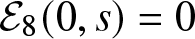 $\mathcal{E}_8(0,s) = 0$.
In case  $t \geq 1$, we apply Lemma 4.1, employ the estimates (11.20) and (11.21), and use that
  $\chi$ is supported on
  $(-k_0,k_0)$ to arrive at
 \begin{equation}
\begin{aligned}
&\left\|\int_0^t |\cdot|^j \mathrm{e}^{\hat{\Lambda}(\cdot)(t-s)} \chi \mathcal{E}_7(\cdot,s)\mathrm{d} s \right\|_{L^1}\\
&\quad \ \leq C_2\left(\int_0^{\frac{t}{2}} \int_{-k_0}^{k_0} \frac{E_0 + \eta(s)^2}{\sqrt{1+s} (\log(2+s))^{\frac23}} |k|^{1+j} \mathrm{e}^{-\frac12 \alpha k^2 (t-s)} \mathrm{d} k \mathrm{d} s\right.\\
&\quad \ \qquad \left. + \, \int_{\frac{t}{2}}^t \int_{-k_0}^{k_0} \frac{E_0 + \eta(s)^2}{(1+s) (\log(2+s))^{\frac23}} |k|^j \mathrm{e}^{-\frac12 \alpha k^2 (t-s)} \mathrm{d} k \mathrm{d} s\right)\\
&\quad \ \leq C_3\left(\int_0^{\frac{t}{2}} \frac{E_0+\eta(s)^2}{\sqrt{t-s}(1+t-s)^{\frac{1+j}{2}}\sqrt{1+s} (\log(2+s))^{\frac23}} \mathrm{d} s\right. \\
&\quad \ \qquad \left. + \, \int_{\frac{t}{2}}^t \frac{E_0 + \eta(s)^2}{\sqrt{t-s}(1+t-s)^{\frac{j}{2}}(1+s) (\log(2+s))^{\frac23}} \mathrm{d} s\right)\\
&\quad \ \leq C_4\frac{E_0 + \eta(t)^2}{(1+t)^{\frac{1+j}{2}} (\log(2+t))^{\frac23- j}},
\end{aligned}
\end{equation}
\begin{equation}
\begin{aligned}
&\left\|\int_0^t |\cdot|^j \mathrm{e}^{\hat{\Lambda}(\cdot)(t-s)} \chi \mathcal{E}_7(\cdot,s)\mathrm{d} s \right\|_{L^1}\\
&\quad \ \leq C_2\left(\int_0^{\frac{t}{2}} \int_{-k_0}^{k_0} \frac{E_0 + \eta(s)^2}{\sqrt{1+s} (\log(2+s))^{\frac23}} |k|^{1+j} \mathrm{e}^{-\frac12 \alpha k^2 (t-s)} \mathrm{d} k \mathrm{d} s\right.\\
&\quad \ \qquad \left. + \, \int_{\frac{t}{2}}^t \int_{-k_0}^{k_0} \frac{E_0 + \eta(s)^2}{(1+s) (\log(2+s))^{\frac23}} |k|^j \mathrm{e}^{-\frac12 \alpha k^2 (t-s)} \mathrm{d} k \mathrm{d} s\right)\\
&\quad \ \leq C_3\left(\int_0^{\frac{t}{2}} \frac{E_0+\eta(s)^2}{\sqrt{t-s}(1+t-s)^{\frac{1+j}{2}}\sqrt{1+s} (\log(2+s))^{\frac23}} \mathrm{d} s\right. \\
&\quad \ \qquad \left. + \, \int_{\frac{t}{2}}^t \frac{E_0 + \eta(s)^2}{\sqrt{t-s}(1+t-s)^{\frac{j}{2}}(1+s) (\log(2+s))^{\frac23}} \mathrm{d} s\right)\\
&\quad \ \leq C_4\frac{E_0 + \eta(t)^2}{(1+t)^{\frac{1+j}{2}} (\log(2+t))^{\frac23- j}},
\end{aligned}
\end{equation}for  $j = 0,1$ and some
  $t$- and
  $E_0$-independent constants
  $C_2,C_3, C_4 \gt 0$. In case
  $t \leq 1$, we use Lemma 4.1, the fact that
  $\chi$ has compact support and estimates (11.20) and (11.21), to establish the short-time bound
 \begin{equation}
\begin{aligned}
\left\||\cdot|^j \int_0^t \mathrm{e}^{\hat{\Lambda}(\cdot)(t-s)} \chi \mathcal{E}_7(\cdot,s)\mathrm{d} s \right\|_{L^1}
&\leq C_2\int_0^t \int_\mathbb{R} \frac{E_0 + \eta(s)^2}{(1+s) (\log(2+s))^{\frac23}} \mathrm{e}^{-\frac12 \alpha k^2 (t-s)} \mathrm{d} k \mathrm{d} s\\
&\leq C_3\int_0^t \frac{E_0 + \eta(s)^2}{\sqrt{t-s}} \mathrm{d} s\\ &\leq C_4\frac{E_0 + \eta(t)^2}{(1+t)^{\frac{1+j}{2}} (\log(2+t))^{\frac23- j}},
\end{aligned}
\end{equation}
\begin{equation}
\begin{aligned}
\left\||\cdot|^j \int_0^t \mathrm{e}^{\hat{\Lambda}(\cdot)(t-s)} \chi \mathcal{E}_7(\cdot,s)\mathrm{d} s \right\|_{L^1}
&\leq C_2\int_0^t \int_\mathbb{R} \frac{E_0 + \eta(s)^2}{(1+s) (\log(2+s))^{\frac23}} \mathrm{e}^{-\frac12 \alpha k^2 (t-s)} \mathrm{d} k \mathrm{d} s\\
&\leq C_3\int_0^t \frac{E_0 + \eta(s)^2}{\sqrt{t-s}} \mathrm{d} s\\ &\leq C_4\frac{E_0 + \eta(t)^2}{(1+t)^{\frac{1+j}{2}} (\log(2+t))^{\frac23- j}},
\end{aligned}
\end{equation}for  $j = 0,1$ and some
  $t$- and
  $E_0$-independent constants
  $C_2,C_3, C_4 \gt 0$. Furthermore, Lemma 4.1, the fact that
  $\chi$ is supported on
  $(-k_0,k_0)$ and estimates (11.20) and (11.21) yield
 \begin{equation}
\begin{aligned}
&\left\||\cdot|^j \partial_k \int_0^t \mathrm{e}^{\hat{\Lambda}(\cdot)(t-s)} \chi \mathcal{E}_7(\cdot,s)\mathrm{d} s \right\|_{L^1}\\
&\quad \ \leq C_2 \int_0^t \int_{-k_0}^{k_0} \frac{\left(E_0 + \eta(t)^2\right)\left(1 + |k|^2 (t-s)\right)}{\sqrt{1+s} (\log(2+s))^{\frac23}} |k|^j\mathrm{e}^{-\frac12 \alpha k^2 (t-s)} \mathrm{d} k \mathrm{d} s\\
&\quad \ \leq C_3\int_0^t \frac{E_0+\eta(s)^2}{\sqrt{t-s} (1+t-s)^{\frac{j}{2}} \sqrt{1+s} (\log(2+s))^{\frac23}} \mathrm{d} s\\
&\quad \ \leq C_4\frac{E_0 + \eta(t)^2}{(1+t)^{\frac{j}{2}}(\log(2+t))^{\frac23-j}},
\end{aligned}
\end{equation}
\begin{equation}
\begin{aligned}
&\left\||\cdot|^j \partial_k \int_0^t \mathrm{e}^{\hat{\Lambda}(\cdot)(t-s)} \chi \mathcal{E}_7(\cdot,s)\mathrm{d} s \right\|_{L^1}\\
&\quad \ \leq C_2 \int_0^t \int_{-k_0}^{k_0} \frac{\left(E_0 + \eta(t)^2\right)\left(1 + |k|^2 (t-s)\right)}{\sqrt{1+s} (\log(2+s))^{\frac23}} |k|^j\mathrm{e}^{-\frac12 \alpha k^2 (t-s)} \mathrm{d} k \mathrm{d} s\\
&\quad \ \leq C_3\int_0^t \frac{E_0+\eta(s)^2}{\sqrt{t-s} (1+t-s)^{\frac{j}{2}} \sqrt{1+s} (\log(2+s))^{\frac23}} \mathrm{d} s\\
&\quad \ \leq C_4\frac{E_0 + \eta(t)^2}{(1+t)^{\frac{j}{2}}(\log(2+t))^{\frac23-j}},
\end{aligned}
\end{equation}for  $j = 0,1$ and some
  $t$- and
  $E_0$-independent constants
  $C_2,C_3, C_4 \gt 0$. Similarly, the
  $L^\infty$-estimate
 \begin{align*}
\left\|\int_0^t |\cdot|^j \mathrm{e}^{\hat{\Lambda}(\cdot)(t-s)} \chi \mathcal{E}_7(\cdot,s)\mathrm{d} s \right\|_{L^\infty}
&\leq C_2\int_0^t \frac{E_0+\eta(s)^2}{\sqrt{t-s} (1+t-s)^{\frac{j}{2}}\sqrt{1+s} (\log(2+s))^{\frac23}} \mathrm{d} s\\ &\leq C_3\frac{E_0 + \eta(t)^2}{(1+t)^{\frac{j}{2}}(\log(2+t))^{\frac23-j}},
\end{align*}
\begin{align*}
\left\|\int_0^t |\cdot|^j \mathrm{e}^{\hat{\Lambda}(\cdot)(t-s)} \chi \mathcal{E}_7(\cdot,s)\mathrm{d} s \right\|_{L^\infty}
&\leq C_2\int_0^t \frac{E_0+\eta(s)^2}{\sqrt{t-s} (1+t-s)^{\frac{j}{2}}\sqrt{1+s} (\log(2+s))^{\frac23}} \mathrm{d} s\\ &\leq C_3\frac{E_0 + \eta(t)^2}{(1+t)^{\frac{j}{2}}(\log(2+t))^{\frac23-j}},
\end{align*}follows for some  $t$- and
  $E_0$-independent constants
  $C_2,C_3 \gt 0$.
We proceed with bounding the linear term in (11.19). By Lemma 4.1, estimate (11.6) the mean value theorem and the facts that 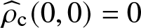 $\widehat{\rho}_{\mathrm{c}}(0,0) = 0$ and that
  $\widehat{\rho}_{\mathrm{c}}(\cdot,0)$ is supported on
  $(-k_0,k_0)$, there exist
  $t$- and
  $E_0$-independent constants
  $C_2,C_3 \gt 0$ such that for
  $p = 1,\infty$ and
  $j = 0,1$, we have
 \begin{equation}
\begin{aligned}
\left\||\cdot|^j \mathrm{e}^{\hat{\Lambda}(\cdot)t} \widehat{\rho}_{\mathrm{c}}(0)\right\|_{L^p} &\leq C_2\left\|\widehat{\rho}_{\mathrm{c}}(0)\right\|_{L^p} \leq C_3 E_0,\\
\left\||\cdot|^j \partial_k \mathrm{e}^{\hat{\Lambda}(\cdot)t} \widehat{\rho}_{\mathrm{c}}(0)\right\|_{L^1} &\leq C_2 \left\|\widehat{\rho}_{\mathrm{c}}(0)\right\|_{W^{1,1}} \leq C_3 E_0,
\end{aligned}
\end{equation}
\begin{equation}
\begin{aligned}
\left\||\cdot|^j \mathrm{e}^{\hat{\Lambda}(\cdot)t} \widehat{\rho}_{\mathrm{c}}(0)\right\|_{L^p} &\leq C_2\left\|\widehat{\rho}_{\mathrm{c}}(0)\right\|_{L^p} \leq C_3 E_0,\\
\left\||\cdot|^j \partial_k \mathrm{e}^{\hat{\Lambda}(\cdot)t} \widehat{\rho}_{\mathrm{c}}(0)\right\|_{L^1} &\leq C_2 \left\|\widehat{\rho}_{\mathrm{c}}(0)\right\|_{W^{1,1}} \leq C_3 E_0,
\end{aligned}
\end{equation}for  $t\leq 1$, and
 \begin{equation}
\begin{aligned}
\left\||\cdot|^j \mathrm{e}^{\hat{\Lambda}(\cdot)t} \widehat{\rho}_{\mathrm{c}}(0)\right\|_{L^1} &\leq C_2 \int_\mathbb{R} |k|^{1+j} \mathrm{e}^{-\frac12 \alpha k^2 t} \left\|\partial_k \widehat{\rho}_{\mathrm{c}}(0)\right\|_{L^\infty} \mathrm{d} k \leq C_3 \frac{E_0}{t^{1+\frac{j}{2}}},\\
\left\||\cdot|^j \mathrm{e}^{\hat{\Lambda}(\cdot)t} \widehat{\rho}_{\mathrm{c}}(0)\right\|_{L^\infty} &\leq C_2 \sup_{k \in \mathbb{R}} |k|^{1+j} \mathrm{e}^{-\frac12 \alpha k^2 t} \left\|\partial_k \widehat{\rho}_{\mathrm{c}}(0)\right\|_{L^\infty} \leq C_3 \frac{E_0}{t^{\frac{1+j}{2}}},\\
\left\||\cdot|^j \partial_k \mathrm{e}^{\hat{\Lambda}(\cdot)t} \widehat{\rho}_{\mathrm{c}}(0)\right\|_{L^1} &\leq C_2\Big(
t \left\||\cdot|^{1+j} \mathrm{e}^{-\frac12 \alpha |\cdot|^2 t} \widehat{\rho}_{\mathrm{c}}(0)\right\|_{L^1}\\
&\qquad \, + \left\| |\cdot|^j \mathrm{e}^{-\frac12 \alpha |\cdot|^2 t} \partial_k \widehat{\rho}_{\mathrm{c}}(0)\right\|_{L^1}\Big) \leq C_3 \frac{E_0}{t^{\frac{1+j}{2}}},
\end{aligned}
\end{equation}
\begin{equation}
\begin{aligned}
\left\||\cdot|^j \mathrm{e}^{\hat{\Lambda}(\cdot)t} \widehat{\rho}_{\mathrm{c}}(0)\right\|_{L^1} &\leq C_2 \int_\mathbb{R} |k|^{1+j} \mathrm{e}^{-\frac12 \alpha k^2 t} \left\|\partial_k \widehat{\rho}_{\mathrm{c}}(0)\right\|_{L^\infty} \mathrm{d} k \leq C_3 \frac{E_0}{t^{1+\frac{j}{2}}},\\
\left\||\cdot|^j \mathrm{e}^{\hat{\Lambda}(\cdot)t} \widehat{\rho}_{\mathrm{c}}(0)\right\|_{L^\infty} &\leq C_2 \sup_{k \in \mathbb{R}} |k|^{1+j} \mathrm{e}^{-\frac12 \alpha k^2 t} \left\|\partial_k \widehat{\rho}_{\mathrm{c}}(0)\right\|_{L^\infty} \leq C_3 \frac{E_0}{t^{\frac{1+j}{2}}},\\
\left\||\cdot|^j \partial_k \mathrm{e}^{\hat{\Lambda}(\cdot)t} \widehat{\rho}_{\mathrm{c}}(0)\right\|_{L^1} &\leq C_2\Big(
t \left\||\cdot|^{1+j} \mathrm{e}^{-\frac12 \alpha |\cdot|^2 t} \widehat{\rho}_{\mathrm{c}}(0)\right\|_{L^1}\\
&\qquad \, + \left\| |\cdot|^j \mathrm{e}^{-\frac12 \alpha |\cdot|^2 t} \partial_k \widehat{\rho}_{\mathrm{c}}(0)\right\|_{L^1}\Big) \leq C_3 \frac{E_0}{t^{\frac{1+j}{2}}},
\end{aligned}
\end{equation}for  $t\geq 1$.
All in all, applying (11.22), (11.23), (11.24) and (11.25)-(11.26) to bound the right-hand side of (11.19) yields a  $t$- and
  $E_0$-independent constant
  $C_* \gt 0$ such that
 \begin{equation}
\big\|\widehat{\rho}_{\mathrm{c}}(t)\big\|_{L^1} \leq \frac{C_*\left(E_0 + \eta(t)^2\right)}{\sqrt{1+t} (\log(2+t))^{\frac23}}, \qquad \big\|\widehat{\rho}_{\mathrm{c}}(t)\big\|_{L^\infty}, \big\|\partial_k \widehat{\rho}_{\mathrm{c}}(t)\big\|_{L^1} \leq\frac{C_*\left(E_0 + \eta(t)^2\right)}{(\log(2+t))^{\frac23}},
\end{equation}
\begin{equation}
\big\|\widehat{\rho}_{\mathrm{c}}(t)\big\|_{L^1} \leq \frac{C_*\left(E_0 + \eta(t)^2\right)}{\sqrt{1+t} (\log(2+t))^{\frac23}}, \qquad \big\|\widehat{\rho}_{\mathrm{c}}(t)\big\|_{L^\infty}, \big\|\partial_k \widehat{\rho}_{\mathrm{c}}(t)\big\|_{L^1} \leq\frac{C_*\left(E_0 + \eta(t)^2\right)}{(\log(2+t))^{\frac23}},
\end{equation}and
 \begin{equation}
\begin{aligned}
\big\||\cdot| \partial_k^j \widehat{\rho}_{\mathrm{c}}(t)\big\|_{L^1} \leq\frac{C_*\left(E_0 + \eta(t)^2\right)(\log(2+t))^{\frac13}}{(1+t)^{1-\frac{j}{2}}},\\
\big\||\cdot| \widehat{\rho}_{\mathrm{c}}(t)\big\|_{L^\infty} \leq\frac{C_*\left(E_0 + \eta(t)^2\right)(\log(2+t))^{\frac13}}{(1+t)^{\frac{1}{2}}},
\end{aligned}
\end{equation}
\begin{equation}
\begin{aligned}
\big\||\cdot| \partial_k^j \widehat{\rho}_{\mathrm{c}}(t)\big\|_{L^1} \leq\frac{C_*\left(E_0 + \eta(t)^2\right)(\log(2+t))^{\frac13}}{(1+t)^{1-\frac{j}{2}}},\\
\big\||\cdot| \widehat{\rho}_{\mathrm{c}}(t)\big\|_{L^\infty} \leq\frac{C_*\left(E_0 + \eta(t)^2\right)(\log(2+t))^{\frac13}}{(1+t)^{\frac{1}{2}}},
\end{aligned}
\end{equation}for  $j = 0,1$.
Bounds on  $\widehat{U}_\mathrm{s}(t)$. Let
  $t \in [0,T_{\max})$ with
  $\eta(t) \leq \eta_0 \leq 1$ and
  $E_0 \in (0,{\varepsilon})$. We derive estimates on
  $\widehat{U}_\mathrm{s}(t)$ by bounding the right-hand side of its Duhamel formula (5.11). Firstly, we apply Lemma 6.1 and obtain a
  $t$- and
  $E_0$-independent constant
  $C_1 \gt 0$ such that
 \begin{equation}
\left\|\partial_k^j \mathcal{F} \mathcal{N}\left(\mathcal{F}^{-1} \widehat{U}(s)\right)\right\|_{L^p} \leq \frac{C_1 \eta(s)^2}{(1+s)^{\frac{1}{2p} + \frac12 (1-j)}},
\end{equation}
\begin{equation}
\left\|\partial_k^j \mathcal{F} \mathcal{N}\left(\mathcal{F}^{-1} \widehat{U}(s)\right)\right\|_{L^p} \leq \frac{C_1 \eta(s)^2}{(1+s)^{\frac{1}{2p} + \frac12 (1-j)}},
\end{equation}for  $j = 0,1$,
  $p = 1, \infty$ and
  $s \in [0,t]$, where we use
  $\eta(t) \leq 1$. Next, we evoke Lemma 4.1 and estimate (11.29) to arrive at
 \begin{equation}
\begin{aligned}
&\left\|\partial_k^j \int_0^t \mathrm{e}^{\hat{\Lambda}(\cdot)(t-s)} (1-\chi) \mathcal{F} \mathcal{N}\left(\mathcal{F}^{-1} \widehat{U}(s)\right) \mathrm{d} s \right\|_{L^p}\\
&\quad \ \leq C_2 \int_0^t \mathrm{e}^{-\theta(t-s)} \left\|\mathcal{F} \mathcal{N}\left(\mathcal{F}^{-1} \widehat{U}(s)\right)\right\|_{W^{j,p}} \mathrm{d} s \\
&\quad \ \leq C_3 \int_0^t \frac{\mathrm{e}^{-\theta(t-s)} \eta(s)^2}{(1+s)^{\frac{1}{2p} + \frac12 (1-j)}} \mathrm{d} s \leq C_4 \frac{\eta(t)^2}{(1+t)^{\frac{1}{2p} + \frac12 (1-j)}},
\end{aligned}
\end{equation}
\begin{equation}
\begin{aligned}
&\left\|\partial_k^j \int_0^t \mathrm{e}^{\hat{\Lambda}(\cdot)(t-s)} (1-\chi) \mathcal{F} \mathcal{N}\left(\mathcal{F}^{-1} \widehat{U}(s)\right) \mathrm{d} s \right\|_{L^p}\\
&\quad \ \leq C_2 \int_0^t \mathrm{e}^{-\theta(t-s)} \left\|\mathcal{F} \mathcal{N}\left(\mathcal{F}^{-1} \widehat{U}(s)\right)\right\|_{W^{j,p}} \mathrm{d} s \\
&\quad \ \leq C_3 \int_0^t \frac{\mathrm{e}^{-\theta(t-s)} \eta(s)^2}{(1+s)^{\frac{1}{2p} + \frac12 (1-j)}} \mathrm{d} s \leq C_4 \frac{\eta(t)^2}{(1+t)^{\frac{1}{2p} + \frac12 (1-j)}},
\end{aligned}
\end{equation}for some  $t$- and
  $E_0$-independent constants
  $C_2,C_3, C_4 \gt 0$. On the other hand, Lemma 4.1 readily yields the linear estimate
 \begin{equation}
\begin{aligned}
\left\|\partial_k^j \mathrm{e}^{\hat{\Lambda}(\cdot)t} (1-\chi)\widehat{U}(0)\right\|_{L^p} \leq C_2 \mathrm{e}^{-\theta t} \|\widehat{U}(0)\|_{W^{j,p}} \leq C_2 \mathrm{e}^{-\theta t} E_0,
\end{aligned}
\end{equation}
\begin{equation}
\begin{aligned}
\left\|\partial_k^j \mathrm{e}^{\hat{\Lambda}(\cdot)t} (1-\chi)\widehat{U}(0)\right\|_{L^p} \leq C_2 \mathrm{e}^{-\theta t} \|\widehat{U}(0)\|_{W^{j,p}} \leq C_2 \mathrm{e}^{-\theta t} E_0,
\end{aligned}
\end{equation}for some  $t$- and
  $E_0$-independent constant
  $C_2 \gt 0$. Thus, applying (11.30) and (11.31) to the right-hand side of (5.11) we obtain a
  $t$- and
  $E_0$-independent constant
  $C_* \gt 0$ such that
 \begin{equation}
\big\|\widehat{U}_\mathrm{s}(t)\big\|_{L^1} \leq C_*\frac{E_0 + \eta(t)^2}{1+t}, \qquad \big\|\widehat{U}_\mathrm{s}(t)\big\|_{L^\infty}, \big\|\partial_k \widehat{U}_\mathrm{s}(t)\big\|_{L^1} \leq C_*\frac{E_0 + \eta(t)^2}{\sqrt{1+t}}.
\end{equation}
\begin{equation}
\big\|\widehat{U}_\mathrm{s}(t)\big\|_{L^1} \leq C_*\frac{E_0 + \eta(t)^2}{1+t}, \qquad \big\|\widehat{U}_\mathrm{s}(t)\big\|_{L^\infty}, \big\|\partial_k \widehat{U}_\mathrm{s}(t)\big\|_{L^1} \leq C_*\frac{E_0 + \eta(t)^2}{\sqrt{1+t}}.
\end{equation} Bounds on  $\widehat{U}_\mathrm{c}(t)$ and
  $\widehat{U}(t)$. Let
  $t \in [0,T_{\max})$ with
  $\eta(t) \leq \eta_0 \leq 1$ and
  $E_0 \in (0,{\varepsilon})$. Applying Lemma 4.1 and using that
  $\chi$ is supported on
  $(-k_0,k_0)$, we deduce
 \begin{align*}
\left\||\cdot|^m \partial_k^j \left(\chi \mathrm{e}^{\hat{\Lambda}(\cdot)(s+1)}\right)\right\|_{L^1} &\lesssim \int_{-k_0}^{k_0} |k|^m (1 + j |k| (s+1)) \mathrm{e}^{-\frac{1}{2} \alpha k^2 (s+1)} \mathrm{d} k \lesssim \frac{1}{(1+s)^{\frac{1}{2} + \frac{m-j}{2}}},\\
\left\||\cdot|^m \left(\chi \mathrm{e}^{\hat{\Lambda}(\cdot)(s+1)}\right)\right\|_{L^\infty} &\lesssim \sup_{k \in (-k_0,k_0)} |k|^m \mathrm{e}^{-\frac{1}{2} \alpha k^2(s+1)} \lesssim \frac{1}{(1+s)^{\frac{m}{2}}}
\end{align*}
\begin{align*}
\left\||\cdot|^m \partial_k^j \left(\chi \mathrm{e}^{\hat{\Lambda}(\cdot)(s+1)}\right)\right\|_{L^1} &\lesssim \int_{-k_0}^{k_0} |k|^m (1 + j |k| (s+1)) \mathrm{e}^{-\frac{1}{2} \alpha k^2 (s+1)} \mathrm{d} k \lesssim \frac{1}{(1+s)^{\frac{1}{2} + \frac{m-j}{2}}},\\
\left\||\cdot|^m \left(\chi \mathrm{e}^{\hat{\Lambda}(\cdot)(s+1)}\right)\right\|_{L^\infty} &\lesssim \sup_{k \in (-k_0,k_0)} |k|^m \mathrm{e}^{-\frac{1}{2} \alpha k^2(s+1)} \lesssim \frac{1}{(1+s)^{\frac{m}{2}}}
\end{align*}for  $s \geq 0$,
  $p = 1,\infty$,
  $j = 0,1$ and
  $m = 0,1$. So, recalling (10.1), (10.2) and (11.5) and employing the estimates (11.18), (11.27) and (11.28), we obtain a
  $t$- and
  $E_0$-independent constant
  $C_1 \gt 0$ such that
 \begin{align*}
\big\||\cdot|^m \widehat{Z}_{\mathrm{c}}(t)\big\|_{L^p} &\leq \big\||\cdot|^m\varsigma_{\mathrm{c}}(t)\big\|_{L^p} + \big\||\cdot|^m \widehat{\rho}_{\mathrm{c}}(t)\big\|_{L^p}\\
&\leq |A(t)| \left\||\cdot|^m \left(\chi \mathrm{e}^{\hat{\Lambda}(\cdot)(t+1)}\right)\right\|_{L^p} + \big\||\cdot|^m \widehat{\rho}_{\mathrm{c}}(t)\big\|_{L^p} \\
&\leq C_1 \frac{\left(E_0 + \eta(t)^{\frac32}\right) (\log(2+t))^{\frac{m}{3}}}{(1+t)^{\frac{1}{2p} + \frac{m}{2}}},
\end{align*}
\begin{align*}
\big\||\cdot|^m \widehat{Z}_{\mathrm{c}}(t)\big\|_{L^p} &\leq \big\||\cdot|^m\varsigma_{\mathrm{c}}(t)\big\|_{L^p} + \big\||\cdot|^m \widehat{\rho}_{\mathrm{c}}(t)\big\|_{L^p}\\
&\leq |A(t)| \left\||\cdot|^m \left(\chi \mathrm{e}^{\hat{\Lambda}(\cdot)(t+1)}\right)\right\|_{L^p} + \big\||\cdot|^m \widehat{\rho}_{\mathrm{c}}(t)\big\|_{L^p} \\
&\leq C_1 \frac{\left(E_0 + \eta(t)^{\frac32}\right) (\log(2+t))^{\frac{m}{3}}}{(1+t)^{\frac{1}{2p} + \frac{m}{2}}},
\end{align*}and
 \begin{align*}
\big\||\cdot|^m \partial_k \widehat{Z}_{\mathrm{c}}(t)\big\|_{L^1} &\leq \big\||\cdot|^m\partial_k \varsigma_{\mathrm{c}}(t)\big\|_{L^1} + \big\||\cdot|^m\partial_k \widehat{\rho}_{\mathrm{c}}(t)\big\|_{L^1}\\
&\leq |A(t)| \left\||\cdot|^m \partial_k \left(\chi \mathrm{e}^{\hat{\Lambda}(\cdot)(t+1)}\right)\right\|_{L^1} + \big\||\cdot|^m \partial_k \widehat{\rho}_{\mathrm{c}}(t)\big\|_{L^1} \\
&\leq C_1 \frac{\left(E_0 + \eta(t)^{\frac32}\right) (\log(2+t))^{\frac{m}{3}}}{(1+t)^{\frac{m}{2}}},
\end{align*}
\begin{align*}
\big\||\cdot|^m \partial_k \widehat{Z}_{\mathrm{c}}(t)\big\|_{L^1} &\leq \big\||\cdot|^m\partial_k \varsigma_{\mathrm{c}}(t)\big\|_{L^1} + \big\||\cdot|^m\partial_k \widehat{\rho}_{\mathrm{c}}(t)\big\|_{L^1}\\
&\leq |A(t)| \left\||\cdot|^m \partial_k \left(\chi \mathrm{e}^{\hat{\Lambda}(\cdot)(t+1)}\right)\right\|_{L^1} + \big\||\cdot|^m \partial_k \widehat{\rho}_{\mathrm{c}}(t)\big\|_{L^1} \\
&\leq C_1 \frac{\left(E_0 + \eta(t)^{\frac32}\right) (\log(2+t))^{\frac{m}{3}}}{(1+t)^{\frac{m}{2}}},
\end{align*}for  $p = 1,\infty$ and
  $m = 0,1$, where we use
  $\eta(t) \leq \eta_0 \leq 1$. Combining the latter with (11.3) we find
  $t$- and
  $E_0$-independent constants
  $C_2,C_3,C_4 \gt 0$ such that
 \begin{equation}
\begin{aligned}
\big\||\cdot|^m \widehat{U}_\mathrm{c}(t)\big\|_{L^p} &\leq C_2\left(\big\||\cdot|^m \widehat{Z}_{\mathrm{c}}(t)\big\|_{L^p} + \big\|\widehat{U}(t)\big\|_{L^1} \big\|\widehat{U}(t)\big\|_{L^p}\right) \\
&\leq C_3 \left(\frac{\left(E_0 + \eta(t)^{\frac32}\right) (\log(2+t))^{\frac{m}{3}}}{(1+t)^{\frac{1}{2p} + \frac{m}{2}}} + \frac{\eta(t)^2}{(1+t)^{\frac12 + \frac1{2p}}}\right)\\
&\leq C_4 \frac{\left(E_0 + \eta(t)^{\frac32}\right) (\log(2+t))^{\frac{m}{3}}}{(1+t)^{\frac{1}{2p} + \frac{m}{2}}},
\end{aligned}
\end{equation}
\begin{equation}
\begin{aligned}
\big\||\cdot|^m \widehat{U}_\mathrm{c}(t)\big\|_{L^p} &\leq C_2\left(\big\||\cdot|^m \widehat{Z}_{\mathrm{c}}(t)\big\|_{L^p} + \big\|\widehat{U}(t)\big\|_{L^1} \big\|\widehat{U}(t)\big\|_{L^p}\right) \\
&\leq C_3 \left(\frac{\left(E_0 + \eta(t)^{\frac32}\right) (\log(2+t))^{\frac{m}{3}}}{(1+t)^{\frac{1}{2p} + \frac{m}{2}}} + \frac{\eta(t)^2}{(1+t)^{\frac12 + \frac1{2p}}}\right)\\
&\leq C_4 \frac{\left(E_0 + \eta(t)^{\frac32}\right) (\log(2+t))^{\frac{m}{3}}}{(1+t)^{\frac{1}{2p} + \frac{m}{2}}},
\end{aligned}
\end{equation}and
 \begin{equation}
\begin{aligned}
\big\||\cdot|^m \partial_k \widehat{U}_\mathrm{c}(t)\big\|_{L^1} &\leq C_2\left(\big\||\cdot|^m \partial_k \widehat{Z}_{\mathrm{c}}(t)\big\|_{L^1} + \big\|\widehat{U}(t)\big\|_{W^{1,1}} \big\|\widehat{U}(t)\big\|_{L^1}\right) \\
&\leq C_3 \left(\frac{\left(E_0 + \eta(t)^{\frac32}\right) (\log(2+t))^{\frac{m}{3}}}{(1+t)^{\frac{m}{2}}} + \frac{\eta(t)^2}{\sqrt{1+t}}\right)\\
&\leq C_4 \frac{\left(E_0 + \eta(t)^{\frac32}\right) (\log(2+t))^{\frac{m}{3}}}{(1+t)^{\frac{m}{2}}},
\end{aligned}
\end{equation}
\begin{equation}
\begin{aligned}
\big\||\cdot|^m \partial_k \widehat{U}_\mathrm{c}(t)\big\|_{L^1} &\leq C_2\left(\big\||\cdot|^m \partial_k \widehat{Z}_{\mathrm{c}}(t)\big\|_{L^1} + \big\|\widehat{U}(t)\big\|_{W^{1,1}} \big\|\widehat{U}(t)\big\|_{L^1}\right) \\
&\leq C_3 \left(\frac{\left(E_0 + \eta(t)^{\frac32}\right) (\log(2+t))^{\frac{m}{3}}}{(1+t)^{\frac{m}{2}}} + \frac{\eta(t)^2}{\sqrt{1+t}}\right)\\
&\leq C_4 \frac{\left(E_0 + \eta(t)^{\frac32}\right) (\log(2+t))^{\frac{m}{3}}}{(1+t)^{\frac{m}{2}}},
\end{aligned}
\end{equation}for  $p = 1,\infty$ and
  $m = 0,1$, where we use
  $\eta(t) \leq \eta_0 \leq 1$. Finally, identity (5.4) and estimates (11.32), (11.33) and (11.34) yield
 \begin{equation}
\big\|\widehat{U}(t)\big\|_{L^1} \leq \frac{C_*\left(E_0 + \eta(t)^{\frac32}\right)}{\sqrt{1+t}}, \qquad \big\|\widehat{U}(t)\big\|_{L^\infty}, \big\|\partial_k \widehat{U}(t)\big\|_{L^1} \leq C_*\left(E_0 + \eta(t)^{\frac32}\right),
\end{equation}
\begin{equation}
\big\|\widehat{U}(t)\big\|_{L^1} \leq \frac{C_*\left(E_0 + \eta(t)^{\frac32}\right)}{\sqrt{1+t}}, \qquad \big\|\widehat{U}(t)\big\|_{L^\infty}, \big\|\partial_k \widehat{U}(t)\big\|_{L^1} \leq C_*\left(E_0 + \eta(t)^{\frac32}\right),
\end{equation}for some  $t$- and
  $E_0$-independent constant
  $C_* \gt 0$.
Proof of key inequality. By the estimates (11.27), (11.32), (11.33), (11.34) and (11.35) there exist  $t$- and
  $E_0$-independent constants
  $C_0,C \gt 0$ such that
 \begin{align*}
\eta(t) \leq C_0\left(E_0 + \eta(t)^{\frac32}\right) \leq C_0\left(E_0 + C_0^{\frac32}\left(E_0 + \eta(t)^{\frac32}\right)^{\frac32}\right) \leq C\left(E_0 + \eta(t)^2\right)
\end{align*}
\begin{align*}
\eta(t) \leq C_0\left(E_0 + \eta(t)^{\frac32}\right) \leq C_0\left(E_0 + C_0^{\frac32}\left(E_0 + \eta(t)^{\frac32}\right)^{\frac32}\right) \leq C\left(E_0 + \eta(t)^2\right)
\end{align*}for  $t \in [0,T_{\max})$ with
  $\eta(t) \leq \eta_0 \leq 1$ and
  $E_0 \in (0,{\varepsilon})$. Therefore, we have established the key inequality (11.8), which, as argued before, implies
  $T_{\max} = \infty$ and
 \begin{equation}
\eta(t) \leq 2CE_0
\end{equation}
\begin{equation}
\eta(t) \leq 2CE_0
\end{equation}for all  $t \geq 0$.
Proof of the estimates (1.10) and (1.11). The estimate (1.10) immediately follows from (11.36) upon taking  $M_0 \geq 2C$. So, all that remains is to establish the pointwise bound (1.11). Recalling (5.4), (9.2) and (10.2), while using Propositions 7.1 and 8.1, we obtain a
  $t$- and
  $E_0$-independent constant
  $C_1 \gt 0$ such that
 \begin{align*}
\left\|\widehat{U}(t) - \varsigma_{\mathrm{c}}(t)\right\|_{L^1} \leq \frac{C_1 E_0}{\sqrt{1+t} (\log(2+t))^{\frac23}}
\end{align*}
\begin{align*}
\left\|\widehat{U}(t) - \varsigma_{\mathrm{c}}(t)\right\|_{L^1} \leq \frac{C_1 E_0}{\sqrt{1+t} (\log(2+t))^{\frac23}}
\end{align*}for  $t \geq 0$. On the other hand, (10.18), (11.5) and (11.18) yield a
  $t$- and
  $E_0$-independent constant
  $C_2 \gt 0$ such that
 \begin{align*}
\left\|P_\pm(0) \varsigma_{\mathrm{c}}(t) - P_\pm(0) \mathrm{e}^{\tilde{\lambda}_\pm(\cdot) (1+t)} A(t)\right\|_{L^1} \leq \frac{C_2}{(1+t)\sqrt{\log(2+t)}}
\end{align*}
\begin{align*}
\left\|P_\pm(0) \varsigma_{\mathrm{c}}(t) - P_\pm(0) \mathrm{e}^{\tilde{\lambda}_\pm(\cdot) (1+t)} A(t)\right\|_{L^1} \leq \frac{C_2}{(1+t)\sqrt{\log(2+t)}}
\end{align*}for  $t \geq 0$, where
  $\tilde{\lambda}_\pm$ is given by (1.21). Using the latter two estimates, we find a
  $t$- and
  $E_0$-independent constant
  $C_3 \gt 0$ such that
 \begin{equation}
\begin{aligned}
&\left|P_\pm(0) U(x,t) - P_\pm(0) \mathcal{F}^{-1}\left(\mathrm{e}^{\tilde{\lambda}_\pm(\cdot) (1+t)}\right)(x) A(t)\right|\\
&\quad \ \leq \left\|P_\pm(0) \widehat{U}(t) - P_\pm(0)\varsigma_{\mathrm{c}}(t)\right\|_{L^1} + \left\|P_\pm(0) \varsigma_{\mathrm{c}}(t) - P_\pm(0) \mathrm{e}^{\tilde{\lambda}_+(\cdot) (1+t)} A(t)\right\|_{L^1}\\
&\quad \ \leq \frac{C_3}{\sqrt{1+t} (\log(2+t))^{\frac23}}
\end{aligned}
\end{equation}
\begin{equation}
\begin{aligned}
&\left|P_\pm(0) U(x,t) - P_\pm(0) \mathcal{F}^{-1}\left(\mathrm{e}^{\tilde{\lambda}_\pm(\cdot) (1+t)}\right)(x) A(t)\right|\\
&\quad \ \leq \left\|P_\pm(0) \widehat{U}(t) - P_\pm(0)\varsigma_{\mathrm{c}}(t)\right\|_{L^1} + \left\|P_\pm(0) \varsigma_{\mathrm{c}}(t) - P_\pm(0) \mathrm{e}^{\tilde{\lambda}_+(\cdot) (1+t)} A(t)\right\|_{L^1}\\
&\quad \ \leq \frac{C_3}{\sqrt{1+t} (\log(2+t))^{\frac23}}
\end{aligned}
\end{equation}for  $x \in \mathbb{R}$ and
  $t \geq 0$. Finally, using the standard integral (10.21), we compute
 \begin{equation}
\mathcal{F}^{-1}\left(\mathrm{e}^{\tilde{\lambda}_\pm(\cdot) (1 + t)}\right)(x) = \frac{1}{2\pi} \int_\mathbb{R} \mathrm{e}^{\tilde{\lambda}_\pm(k) (1+t) + \mathrm{i} k x} \mathrm{d} k = \frac{\mathrm{e}^{\pm \mathrm{i} (1+t) - \frac{x^2}{2(\alpha \mp \mathrm{i}) (1+t)}}}{\sqrt{2\pi(\alpha \mp \mathrm{i})(1+t)}}
\end{equation}
\begin{equation}
\mathcal{F}^{-1}\left(\mathrm{e}^{\tilde{\lambda}_\pm(\cdot) (1 + t)}\right)(x) = \frac{1}{2\pi} \int_\mathbb{R} \mathrm{e}^{\tilde{\lambda}_\pm(k) (1+t) + \mathrm{i} k x} \mathrm{d} k = \frac{\mathrm{e}^{\pm \mathrm{i} (1+t) - \frac{x^2}{2(\alpha \mp \mathrm{i}) (1+t)}}}{\sqrt{2\pi(\alpha \mp \mathrm{i})(1+t)}}
\end{equation}for  $x \in \mathbb{R}$ and
  $t \geq 0$. Combining the latter with (11.5), (11.18) and (11.37), we arrive at the pointwise bound (1.11), which finishes the proof.
Thanks to the pointwise estimate (11.37), established in the proof of Theorem 1.1, it suffices to obtain a leading-order expression for  $(P_\pm(0) A(t))_1 = r_\pm(t) \mathrm{e}^{\mathrm{i} \psi_\pm t}$ in order to prove Theorem 1.2. To this end, we approximate
  $(r_\pm(t),\psi_\pm(t))$ by the solution
  $(\tilde{r}_\pm(t),\tilde{\psi}_\pm(t))$ to the reduced ODE (10.27) with initial condition
  $(\tilde{r}_\pm(0),\tilde{\psi}_\pm(0)) = (r_\pm(0),\psi_\pm(0))$, which is explicitly given by (10.28). The approximation of
  $r_\pm(t)$ is obtained by applying a nonlinear iteration argument to (10.25), after first separating variables and integrating the equation. On the other hand, the approximation of
  $\psi_\pm(t)$ follows from integrating (10.26) and directly estimating the difference
  $\psi_\pm(t) - \tilde{\psi}_\pm(t)$.
Proof of Theorem 1.2
Let  ${\varepsilon} \gt 0$ be as in Theorem 1.1. Take
  $\delta \gt 0$ such that
 \begin{equation}
E_0 \overset{\scriptscriptstyle{\mathrm{def}}}{=} \delta \big(\|\hat{u}_*\|_{W^{1,1} \cap W^{1,\infty}} + \|\hat{w}_*\|_{W^{1,1} \cap W^{1,\infty}}\big) \lt {\varepsilon},
\end{equation}
\begin{equation}
E_0 \overset{\scriptscriptstyle{\mathrm{def}}}{=} \delta \big(\|\hat{u}_*\|_{W^{1,1} \cap W^{1,\infty}} + \|\hat{w}_*\|_{W^{1,1} \cap W^{1,\infty}}\big) \lt {\varepsilon},
\end{equation}so that the identities in the proof of Theorem 1.1 hold true. By (4.4), (5.1), (5.4), (10.1), (10.24), (11.3) and (11.39), there exists a  $\delta$-independent constant
  $C_1 \gt 0$ such that
 \begin{align*}
\big|P_+(0)\widehat{Z}_{\mathrm{c}}(0,0) - \delta U_*\big|, \big|P_-(0)\widehat{Z}_{\mathrm{c}}(0,0) - \delta \overline{U_*}\big| \leq C_1 \delta^2,
\end{align*}
\begin{align*}
\big|P_+(0)\widehat{Z}_{\mathrm{c}}(0,0) - \delta U_*\big|, \big|P_-(0)\widehat{Z}_{\mathrm{c}}(0,0) - \delta \overline{U_*}\big| \leq C_1 \delta^2,
\end{align*}and
 \begin{equation}
\big|r_\pm(0) - \delta |U_*|\big| \leq C_1 \delta^2, \qquad \big|\psi_\pm(0) \mp 1 \mp \arg(U_*)\big| \leq C_1 \delta.
\end{equation}
\begin{equation}
\big|r_\pm(0) - \delta |U_*|\big| \leq C_1 \delta^2, \qquad \big|\psi_\pm(0) \mp 1 \mp \arg(U_*)\big| \leq C_1 \delta.
\end{equation} Since  $U_* \neq 0$, we conclude, by taking
  $\delta \gt 0$ smaller if necessary, that
  $r_\pm(0) \gt 0$.
The solution  $(\tilde{r}_\pm(t),\tilde{\psi}_\pm(t))$ to the reduced ODE (10.27) with initial condition
  $\tilde{r}_\pm(0) = r_\pm(0)$ and
  $\tilde{\psi}_\pm(0) = \psi_\pm(0)$ is globally defined and explicitly given by (10.28). Moreover, since
  $r_\pm(0) \gt 0$, we have that
  $\tilde{r}_\pm(t)$ is positive for each
  $t \geq 0$ and strictly decreasing. In the following, we approximate
  $(r_\pm(t),\psi_\pm(t))$ by the solution
  $(\tilde{r}_\pm(t),\tilde{\psi}_\pm(t))$.
Approximation of  $r_\pm(t)$. In order to approximate
  $r_\pm(t)$ by
  $\tilde{r}_\pm(t)$, we use the template function
  $\tilde\eta \colon [0,\widetilde{T}_{\max}) \to \mathbb{R}$ given by
 \begin{align*}
\tilde\eta(t) = \sup_{0 \leq s \leq t} \tilde{r}_\pm(s)^2 \big|r_\pm(s)^{-2} - \tilde{r}_\pm(s)^{-2}\big|
\end{align*}
\begin{align*}
\tilde\eta(t) = \sup_{0 \leq s \leq t} \tilde{r}_\pm(s)^2 \big|r_\pm(s)^{-2} - \tilde{r}_\pm(s)^{-2}\big|
\end{align*}where we denote
 \begin{align*} \widetilde{T}_{\max} = \sup\big\{t \in [0,\infty) : r_\pm(s) \gt 0 \text{for } s \in [0,t]\big\} \in (0,\infty].\end{align*}
 Clearly,  $\eta$ is well-defined, continuous and monotonically increasing with
  $\tilde\eta(0) = 0$. Furthermore, if
  $\widetilde{T}_{\max} \lt \infty$, it holds
 \begin{equation}
\lim_{t \uparrow \widetilde{T}_{\max}} \tilde\eta(t) = \infty.
\end{equation}
\begin{equation}
\lim_{t \uparrow \widetilde{T}_{\max}} \tilde\eta(t) = \infty.
\end{equation} Take  $t \in [0,\widetilde{T}_{\max})$ with
  $\tilde\eta(t) \leq 1$. Integrating (10.29) from
  $0$ to
  $t$ and using
 \begin{equation}
\tilde{r}_\pm(s)^{-2} = r_\pm(0)^{-2} - 2\operatorname{Re}(\omega_\pm) \log(s+1)
\end{equation}
\begin{equation}
\tilde{r}_\pm(s)^{-2} = r_\pm(0)^{-2} - 2\operatorname{Re}(\omega_\pm) \log(s+1)
\end{equation}for  $s \geq 0$, we arrive at
 \begin{equation}
r_\pm(t)^{-2} - \tilde{r}_\pm(t)^{-2} = -2\int_0^t \operatorname{Re}\left(\frac{\mathrm{e}^{-\mathrm{i} \psi_\pm(s) \mp \mathrm{i} (s+1)}}{r_\pm(s)^3} \left(P_\pm(0) \mathcal{E}_4(0,s) + \mathcal{E}_6(s)\right)_1\right) \mathrm{d} s.
\end{equation}
\begin{equation}
r_\pm(t)^{-2} - \tilde{r}_\pm(t)^{-2} = -2\int_0^t \operatorname{Re}\left(\frac{\mathrm{e}^{-\mathrm{i} \psi_\pm(s) \mp \mathrm{i} (s+1)}}{r_\pm(s)^3} \left(P_\pm(0) \mathcal{E}_4(0,s) + \mathcal{E}_6(s)\right)_1\right) \mathrm{d} s.
\end{equation} Firstly, we employ (11.40) to bound the right-hand side of (11.42) and obtain a  $\delta$-independent constant
  $C_2 \gt 0$ such that
 \begin{equation}
\tilde{r}_\pm(s)^{-1} \leq C_2 \left(\delta^{-1} + (\log(1+s))^{\frac12}\right)
\end{equation}
\begin{equation}
\tilde{r}_\pm(s)^{-1} \leq C_2 \left(\delta^{-1} + (\log(1+s))^{\frac12}\right)
\end{equation}for  $s \geq 0$. Next, applying (11.13), (11.18), (11.36), (11.39) and (11.44), recalling
  $\tilde{\eta}(t) \leq 1$ and noting that
  $\tilde{r}_\pm(s)^{-2}$ is strictly increasing, we bound the right-hand side of (11.43) as
 \begin{align*}
&\left|\int_0^t \operatorname{Re}\left(\frac{\mathrm{e}^{-\mathrm{i} \psi_\pm(s) \mp \mathrm{i} (s+1)}}{r_\pm(s)^3} \left(P_\pm(0) \mathcal{E}_4(0,s) + \mathcal{E}_6(s)\right)_1\right) \mathrm{d} s\right|\\
&\quad \ \leq C_3 \tilde{r}_\pm(t)^{-2} \left(\int_0^t \frac{\delta^2 \left(\delta^{-1} + \log(1+s)^{\frac12}\right) }{(1+s) (\log(2+s))^2} \mathrm{d} s + \int_0^t \frac{\delta }{(1+s) (\log(2+s))^{\frac23}(\log(1+s))^{\frac12}} \mathrm{d} s\right)\\
&\quad \ \leq C_4 \delta \tilde{r}_\pm(t)^{-2}
\end{align*}
\begin{align*}
&\left|\int_0^t \operatorname{Re}\left(\frac{\mathrm{e}^{-\mathrm{i} \psi_\pm(s) \mp \mathrm{i} (s+1)}}{r_\pm(s)^3} \left(P_\pm(0) \mathcal{E}_4(0,s) + \mathcal{E}_6(s)\right)_1\right) \mathrm{d} s\right|\\
&\quad \ \leq C_3 \tilde{r}_\pm(t)^{-2} \left(\int_0^t \frac{\delta^2 \left(\delta^{-1} + \log(1+s)^{\frac12}\right) }{(1+s) (\log(2+s))^2} \mathrm{d} s + \int_0^t \frac{\delta }{(1+s) (\log(2+s))^{\frac23}(\log(1+s))^{\frac12}} \mathrm{d} s\right)\\
&\quad \ \leq C_4 \delta \tilde{r}_\pm(t)^{-2}
\end{align*}for some  $t$- and
  $\delta$-independent constants
  $C_{3,4} \gt 0$. Hence, multiplying (11.43) with
  $\tilde{r}_\pm(t)^2$, taking suprema and using the previous bound, we establish
 \begin{equation}
\tilde\eta(t) \leq C_4 \delta
\end{equation}
\begin{equation}
\tilde\eta(t) \leq C_4 \delta
\end{equation}for  $t \in [0,\widetilde{T}_{\max})$ with
  $\tilde\eta(t) \leq 1$. By continuity of
  $\tilde\eta$ and the fact that
  $\tilde\eta(0) = 0$, it follows, provided
  $\delta \gt 0$ is sufficiently small, that (11.45) holds for all
  $t \in [0,\smash{\widetilde{T}_{\max}})$. Since this contradicts (11.41), we must have
  $\smash{\widetilde{T}}_{\max} = \infty$. The bound (11.45) yields a
  $\delta$-independent constant
 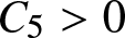 $C_5 \gt 0$ such that
 \begin{equation}
\left|r_\pm(t) - \tilde{r}_\pm(t)\right| \leq C_5 \delta \tilde{r}_\pm(t), \qquad \left|r_\pm(t)^2 - \tilde{r}_\pm(t)^2\right| \leq C_5 \delta \tilde{r}_\pm(t)^2
\end{equation}
\begin{equation}
\left|r_\pm(t) - \tilde{r}_\pm(t)\right| \leq C_5 \delta \tilde{r}_\pm(t), \qquad \left|r_\pm(t)^2 - \tilde{r}_\pm(t)^2\right| \leq C_5 \delta \tilde{r}_\pm(t)^2
\end{equation}for all  $t \geq 0$.
Approximation of  $\psi_\pm(t)$. Since
  $\widetilde{T}_{\max} = \infty$, we have
 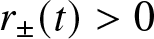 $r_\pm(t) \gt 0$ for all
  $t \geq 0$. Thus, dividing (10.26) by
  $r_\pm(t)$ are integrating from
  $0$ to
  $t$, we infer
 \begin{equation}
\psi_\pm(t) - \tilde{\psi}_\pm(t) = \int_0^t \operatorname{Im}\left(\frac{\omega_\pm}{1+s} \left(r_\pm(s)^2 - \tilde{r}_\pm(s)^2\right) + \frac{\left(P_\pm(0) \mathcal{E}_4(0,s) + \mathcal{E}_6(s)\right)_1}{\mathrm{e}^{\mathrm{i} \psi_\pm(s) \pm \mathrm{i} (s+1)} \, r_\pm(s)} \right) \mathrm{d} s
\end{equation}
\begin{equation}
\psi_\pm(t) - \tilde{\psi}_\pm(t) = \int_0^t \operatorname{Im}\left(\frac{\omega_\pm}{1+s} \left(r_\pm(s)^2 - \tilde{r}_\pm(s)^2\right) + \frac{\left(P_\pm(0) \mathcal{E}_4(0,s) + \mathcal{E}_6(s)\right)_1}{\mathrm{e}^{\mathrm{i} \psi_\pm(s) \pm \mathrm{i} (s+1)} \, r_\pm(s)} \right) \mathrm{d} s
\end{equation}for  $t \geq 0$. Using (11.13), (11.18), (11.36), (11.39), (11.40), (11.44) and (11.46), we bound the right-hand side of (11.47) as
 \begin{equation}
\begin{aligned}
&\left|\int_0^t \operatorname{Im}\left(\frac{\omega_\pm}{1+s} \left(r_\pm(s)^2 - \tilde{r}_\pm(s)^2\right) + \mathrm{e}^{-\mathrm{i} \psi_\pm(s) \mp \mathrm{i} (s+1)}\left(P_\pm(0) \mathcal{E}_4(0,s) + \mathcal{E}_6(s)\right)_1 \right) \mathrm{d} s\right|\\
&\quad \ \leq C_6 \int_0^t \left(\frac{\delta \tilde{r}_\pm(s)^2}{1+s} + \frac{\delta^2 \left(\delta^{-1} + \log(1+s)^{\frac12}\right) }{(1+s) (\log(2+s))^2} + \frac{\delta }{(1+s) (\log(2+s))^{\frac23}(\log(1+s))^{\frac12}} \right) \mathrm{d} s\\
&\quad \ \leq C_7 \delta \left(1 + \log\left(1-2 \operatorname{Re}(\omega_\pm) r_\pm(0)^2 \log (t+1)\right)\right),
\end{aligned}
\end{equation}
\begin{equation}
\begin{aligned}
&\left|\int_0^t \operatorname{Im}\left(\frac{\omega_\pm}{1+s} \left(r_\pm(s)^2 - \tilde{r}_\pm(s)^2\right) + \mathrm{e}^{-\mathrm{i} \psi_\pm(s) \mp \mathrm{i} (s+1)}\left(P_\pm(0) \mathcal{E}_4(0,s) + \mathcal{E}_6(s)\right)_1 \right) \mathrm{d} s\right|\\
&\quad \ \leq C_6 \int_0^t \left(\frac{\delta \tilde{r}_\pm(s)^2}{1+s} + \frac{\delta^2 \left(\delta^{-1} + \log(1+s)^{\frac12}\right) }{(1+s) (\log(2+s))^2} + \frac{\delta }{(1+s) (\log(2+s))^{\frac23}(\log(1+s))^{\frac12}} \right) \mathrm{d} s\\
&\quad \ \leq C_7 \delta \left(1 + \log\left(1-2 \operatorname{Re}(\omega_\pm) r_\pm(0)^2 \log (t+1)\right)\right),
\end{aligned}
\end{equation}yielding
 \begin{equation}
\big|\psi_\pm(t) - \tilde{\psi}_\pm(t)\big| \leq C_8 \delta \left(1 + |\tilde{\psi}_\pm(t) - 1|\right)
\end{equation}
\begin{equation}
\big|\psi_\pm(t) - \tilde{\psi}_\pm(t)\big| \leq C_8 \delta \left(1 + |\tilde{\psi}_\pm(t) - 1|\right)
\end{equation}for  $t \geq 0$, where
  $C_6,C_7,C_8 \gt 0$ are
  $\delta$- and
  $t$-independent constants.
Conclusion. Finally, setting  $r(t) = r_+(t)$,
  $\tilde{r}(t) = \tilde{r}_+(t)$,
  $\psi(t)= \psi_+(t) - 1$ and
  $\tilde{\psi}(t) = \tilde{\psi}_+(t) - 1$, the bounds (11.40), (11.46) and (11.49) yield (1.15). On the other hand, the approximation (1.14) follows by combining (4.4), (10.24), (11.37) and (11.38).
Finally, we state the proof of Theorem 1.3, which relies on an iteration argument in the variables  $\widehat{U}$,
  $\widehat{U}_\mathrm{s}$ and
  $\widehat{Z}_{\mathrm{c}}$ using
  $L^1$-
 $L^\infty$-estimates.
Proof of Theorem 1.3
We close a nonlinear argument controlling the variables  $\widehat{U}(k,t)$,
  $\widehat{Z}_{\mathrm{c}}(k,t)$ and
  $\widehat{U}_\mathrm{s}(k,t) = (1-\chi(k))\widehat{U}(k,t)$.
Template function. Using (3.3), (5.2), (5.7) and (9.4), we observe that the template function  $\eta \colon [0,T_{\max}) \to \mathbb{R}$ given by
 \begin{align*}
\eta(t) &= \sup_{0 \leq s \leq t} \left[\big\|\widehat{U}(s)\big\|_{L^\infty} + \big\|\widehat{Z}_{\mathrm{c}}(s)\big\|_{L^\infty} + \sqrt{1+s}\left(\big\|\widehat{U}(s)\big\|_{L^1} + \big\|\widehat{Z}_{\mathrm{c}}(s)\big\|_{L^1} + \big\|\widehat{U}_\mathrm{s}(s)\big\|_{L^\infty}\right)\right. \\
&\qquad \left. + \, (1+s)\big\|\widehat{U}_\mathrm{s}(s)\big\|_{L^1}\right],
\end{align*}
\begin{align*}
\eta(t) &= \sup_{0 \leq s \leq t} \left[\big\|\widehat{U}(s)\big\|_{L^\infty} + \big\|\widehat{Z}_{\mathrm{c}}(s)\big\|_{L^\infty} + \sqrt{1+s}\left(\big\|\widehat{U}(s)\big\|_{L^1} + \big\|\widehat{Z}_{\mathrm{c}}(s)\big\|_{L^1} + \big\|\widehat{U}_\mathrm{s}(s)\big\|_{L^\infty}\right)\right. \\
&\qquad \left. + \, (1+s)\big\|\widehat{U}_\mathrm{s}(s)\big\|_{L^1}\right],
\end{align*}is well-defined, continuous, monotonically increasing and, if  $T_{\max} \lt \infty$, then we have
 \begin{equation}
\lim_{t \uparrow T_{\max}} \eta(t) = \infty.
\end{equation}
\begin{equation}
\lim_{t \uparrow T_{\max}} \eta(t) = \infty.
\end{equation} Analogous to the proof of Theorem 1.1, we establish the estimates (11.2), (11.3) and (11.4) for  $j,m = 0$. Combining these with (5.1), we find an
  $E_0$-independent constant
  $K_0 \geq 1$ such that
 \begin{equation}
\eta(0) \leq K_0 E_0.
\end{equation}
\begin{equation}
\eta(0) \leq K_0 E_0.
\end{equation} Key inequality. Our aim is to establish a constant  $C \geq K_0$ such that for each
  $t \in [0,T_{\max}) \cap [0,T_{\varepsilon}]$ with
  $\eta(t) \leq 1$ the key inequality
 \begin{equation}
\eta(t) \leq C\left(E_0 + \eta(t)^2 \log(2+t)\right),
\end{equation}
\begin{equation}
\eta(t) \leq C\left(E_0 + \eta(t)^2 \log(2+t)\right),
\end{equation}is satisfied. Then, taking
 \begin{equation*}{\varepsilon} \lt \frac{1}{4C^2}, \qquad M_0 = 2C,\end{equation*}
it follows, by the continuity of  $\eta$, that, provided
  $E_0 \in (0,{\varepsilon})$, it holds
  $\eta(t) \leq M_0E_0 = 2CE_0 \leq 1$ for all
  $t \in [0,T_{\max}) \cap \big[0,T_\varepsilon\big]$. Indeed, given
  $t \in [0,T_{\max}) \cap \big[0,T_\varepsilon\big]$ with
  $\eta(t) \gt 2CE_0$, there must, by continuity of
  $\eta$ and the fact that
  $\eta(0) \lt 2CE_0$ by (11.51), exist
  $s \in (0,t]$ with
  $\eta(s) = 2CE_0 \leq 1$. We arrive at the contradiction
 \begin{equation*}\eta(s) \leq C\left(E_0 + 4C^2E_0^2\log(2+s)\right) \lt 2CE_0,\end{equation*}
by applying estimate (11.52) and the fact that we have  $4C^2 E_0\log(2+s) \lt 1$ for
  $s \leq T_{\varepsilon} = \mathrm{e}^{{\varepsilon}/E_0} - 2$. We conclude that, if (11.52) holds, then
  $\eta(t) \leq 2CE_0$, for all
  $t \in [0,T_{\max}) \cap \big[0,T_\varepsilon\big]$, which implies by (11.50) that
  $T_{\max} \gt T_\varepsilon$. Consequently, we have
  $\eta(t) \leq M_0E_0$ for all
  $t \in \big[0,T_\varepsilon\big]$, which readily yields the desired estimates. So, all that remains is to establish the key inequality (11.52).
Bounds on  $\widehat{Z}_{\mathrm{c}}(t)$. Let
  $t \in [0,T_{\max})$ with
  $\eta(t) \leq 1$ and
  $E_0 \in (0,{\varepsilon})$. We establish estimates on
  $\widehat{Z}_{\mathrm{c}}(t)$ by estimating the terms on the right-hand side of its Duhamel formulation (9.1). Firstly, Lemmas 9.1 and 9.2 and the estimate (11.2) with
  $j,m=0$ yield a
  $t$- and
  $E_0$-independent constant
  $C_1 \gt 0$ such that
 \begin{equation}
\begin{aligned}
\left\|\mathcal{E}_4(\cdot,s)\right\|_{L^\infty}, \left\|Z_3^{\mathrm{res}}(\widehat{Z}_{\mathrm{c}}(s),\widehat{Z}_{\mathrm{c}}(s),\widehat{Z}_{\mathrm{c}}(s))\right\|_{L^\infty} &\leq C_1\frac{\eta(s)^2}{1+s},
\end{aligned}
\end{equation}
\begin{equation}
\begin{aligned}
\left\|\mathcal{E}_4(\cdot,s)\right\|_{L^\infty}, \left\|Z_3^{\mathrm{res}}(\widehat{Z}_{\mathrm{c}}(s),\widehat{Z}_{\mathrm{c}}(s),\widehat{Z}_{\mathrm{c}}(s))\right\|_{L^\infty} &\leq C_1\frac{\eta(s)^2}{1+s},
\end{aligned}
\end{equation}for  $s \in [0,t]$, where we use
  $\eta(t) \leq 1$. On the one hand, Lemma 4.1 and estimate (11.53) yield
 \begin{equation}
\begin{aligned}
&\left\|\int_0^t \mathrm{e}^{\hat{\Lambda}(\cdot)(t-s)} \chi \left(Z_3^{\mathrm{res}}(\widehat{Z}_{\mathrm{c}}(s),\widehat{Z}_{\mathrm{c}}(s),\widehat{Z}_{\mathrm{c}}(s)) + \mathcal{E}_4(\cdot,s)\right) \mathrm{d} s \right\|_{L^1}\\
&\quad \ \leq C_2 \int_0^t \frac{\eta(s)^2}{1+s} \int_\mathbb{R} \mathrm{e}^{-\frac12 \alpha k^2 (t-s)} \mathrm{d} k \mathrm{d} s \\
&\quad \ \leq C_3 \int_0^t \frac{\eta(s)^2}{\sqrt{t-s} (1+s)} \mathrm{d} s \leq C_4 \frac{\eta(t)^2\log(2+t)}{\sqrt{1+t}},
\end{aligned}
\end{equation}
\begin{equation}
\begin{aligned}
&\left\|\int_0^t \mathrm{e}^{\hat{\Lambda}(\cdot)(t-s)} \chi \left(Z_3^{\mathrm{res}}(\widehat{Z}_{\mathrm{c}}(s),\widehat{Z}_{\mathrm{c}}(s),\widehat{Z}_{\mathrm{c}}(s)) + \mathcal{E}_4(\cdot,s)\right) \mathrm{d} s \right\|_{L^1}\\
&\quad \ \leq C_2 \int_0^t \frac{\eta(s)^2}{1+s} \int_\mathbb{R} \mathrm{e}^{-\frac12 \alpha k^2 (t-s)} \mathrm{d} k \mathrm{d} s \\
&\quad \ \leq C_3 \int_0^t \frac{\eta(s)^2}{\sqrt{t-s} (1+s)} \mathrm{d} s \leq C_4 \frac{\eta(t)^2\log(2+t)}{\sqrt{1+t}},
\end{aligned}
\end{equation}and
 \begin{equation}
\begin{aligned}
&\left\|\int_0^t \mathrm{e}^{\hat{\Lambda}(\cdot)(t-s)} \chi \left(Z_3^{\mathrm{res}}(\widehat{Z}_{\mathrm{c}}(s),\widehat{Z}_{\mathrm{c}}(s),\widehat{Z}_{\mathrm{c}}(s)) + \mathcal{E}_4(\cdot,s)\right) \mathrm{d} s \right\|_{L^\infty}\\
&\quad \ \leq C_2 \int_0^t \frac{\eta(s)^2}{1+s} \mathrm{d} s \leq C_3 \eta(t)^2\log(2+t)
\end{aligned}
\end{equation}
\begin{equation}
\begin{aligned}
&\left\|\int_0^t \mathrm{e}^{\hat{\Lambda}(\cdot)(t-s)} \chi \left(Z_3^{\mathrm{res}}(\widehat{Z}_{\mathrm{c}}(s),\widehat{Z}_{\mathrm{c}}(s),\widehat{Z}_{\mathrm{c}}(s)) + \mathcal{E}_4(\cdot,s)\right) \mathrm{d} s \right\|_{L^\infty}\\
&\quad \ \leq C_2 \int_0^t \frac{\eta(s)^2}{1+s} \mathrm{d} s \leq C_3 \eta(t)^2\log(2+t)
\end{aligned}
\end{equation}for some  $t$- and
  $E_0$-independent constants
  $C_2,C_3, C_4 \gt 0$. On the other hand, Lemma 4.1, estimate (11.4) with
  $j = 0$ and the fact that
  $\widehat{Z}_{\mathrm{c}}(\cdot,0)$ is supported on
  $(-k_0,k_0)$, affords the linear estimates
 \begin{equation}
\begin{aligned}
\left\|\mathrm{e}^{\hat{\Lambda}(\cdot)t} \widehat{Z}_{\mathrm{c}}(0)\right\|_{L^1} &\leq C_2 \int_\mathbb{R} \mathrm{e}^{-\frac12 \alpha k^2 t} \mathrm{d} k \big\|\widehat{U}(0)\big\|_{L^\infty} \leq C_3 \frac{E_0}{\sqrt{t}},\\
\left\|\mathrm{e}^{\hat{\Lambda}(\cdot)t} \widehat{Z}_{\mathrm{c}}(0)\right\|_{L^p} &\leq C_2 \big\|\widehat{U}(0)\big\|_{L^p} \leq C_3 E_0,
\end{aligned}
\end{equation}
\begin{equation}
\begin{aligned}
\left\|\mathrm{e}^{\hat{\Lambda}(\cdot)t} \widehat{Z}_{\mathrm{c}}(0)\right\|_{L^1} &\leq C_2 \int_\mathbb{R} \mathrm{e}^{-\frac12 \alpha k^2 t} \mathrm{d} k \big\|\widehat{U}(0)\big\|_{L^\infty} \leq C_3 \frac{E_0}{\sqrt{t}},\\
\left\|\mathrm{e}^{\hat{\Lambda}(\cdot)t} \widehat{Z}_{\mathrm{c}}(0)\right\|_{L^p} &\leq C_2 \big\|\widehat{U}(0)\big\|_{L^p} \leq C_3 E_0,
\end{aligned}
\end{equation}for  $p = 1,\infty$ and some
  $t$- and
  $E_0$-independent constants
  $C_2,C_3 \gt 0$. Thus, applying (11.54), (11.55) and (11.56) to the right-hand side of (9.1), we obtain a
  $t$- and
  $E_0$-independent constant
  $C_* \gt 0$ such that
 \begin{equation}
\big\|\widehat{Z}_{\mathrm{c}}(t)\big\|_{L^1} \leq C_*\frac{\eta(t)^2\log(2+t)}{\sqrt{1+t}}, \qquad \big\|\widehat{Z}_{\mathrm{c}}(t)\big\|_{L^\infty} \leq C_*\eta(t)^2\log(2+t).
\end{equation}
\begin{equation}
\big\|\widehat{Z}_{\mathrm{c}}(t)\big\|_{L^1} \leq C_*\frac{\eta(t)^2\log(2+t)}{\sqrt{1+t}}, \qquad \big\|\widehat{Z}_{\mathrm{c}}(t)\big\|_{L^\infty} \leq C_*\eta(t)^2\log(2+t).
\end{equation} Bounds on  $\widehat{U}_\mathrm{s}(t)$. Let
  $t \in [0,T_{\max})$ with
  $\eta(t) \leq 1$ and
  $E_0 \in (0,{\varepsilon})$. We obtain bounds on
  $\widehat{U}_\mathrm{s}(t)$, which satisfy the Duhamel formula (5.11). Firstly, Lemma 6.1 provides a
  $t$- and
  $E_0$-independent constant
  $C_1 \gt 0$ such that
 \begin{equation}
\left\|\mathcal{F} \mathcal{N}\left(\mathcal{F}^{-1} \widehat{U}(s)\right)\right\|_{L^p} \leq \frac{C_1 \eta(s)^2}{(1+s)^{\frac12 + \frac{1}{2p}}},
\end{equation}
\begin{equation}
\left\|\mathcal{F} \mathcal{N}\left(\mathcal{F}^{-1} \widehat{U}(s)\right)\right\|_{L^p} \leq \frac{C_1 \eta(s)^2}{(1+s)^{\frac12 + \frac{1}{2p}}},
\end{equation}for  $p = 1, \infty$ and
  $s \in [0,t]$, where we use
  $\eta(t) \leq 1$. Analogous to the proof of Theorem 1.1, we derive the estimates (11.30) and (11.31) for
  $j = 0$ and
  $p = 1,\infty$ using Lemma 4.1 and estimate (11.58). Thus, applying (11.30) and (11.31) to the right-hand side of (5.11), we arrive at
 \begin{equation}
\big\|\widehat{U}_\mathrm{s}(t)\big\|_{L^1} \leq C_*\frac{E_0 + \eta(t)^2}{1+t}, \qquad \big\|\widehat{U}_\mathrm{s}(t)\big\|_{L^\infty} \leq C_*\frac{E_0 + \eta(t)^2}{\sqrt{1+t}},
\end{equation}
\begin{equation}
\big\|\widehat{U}_\mathrm{s}(t)\big\|_{L^1} \leq C_*\frac{E_0 + \eta(t)^2}{1+t}, \qquad \big\|\widehat{U}_\mathrm{s}(t)\big\|_{L^\infty} \leq C_*\frac{E_0 + \eta(t)^2}{\sqrt{1+t}},
\end{equation}for some  $t$- and
  $E_0$-independent constant
  $C_* \gt 0$.
Bounds on  $\widehat{U}(t)$. Let
  $t \in [0,T_{\max})$ with
  $\eta(t) \leq 1$ and
  $E_0 \in (0,{\varepsilon})$. We apply estimate (11.3) with
  $j = 0$ and the bound (11.57) to find
  $t$- and
  $E_0$-independent constants
  $C_2,C_3,C_4 \gt 0$ such that
 \begin{equation}
\begin{aligned}
\big\|\widehat{U}_\mathrm{c}(t)\big\|_{L^p} &\leq C_2\left(\big\|\widehat{Z}_{\mathrm{c}}(t)\big\|_{L^p} + \big\|\widehat{U}(t)\big\|_{L^1} \big\|\widehat{U}(t)\big\|_{L^p}\right) \\
&\leq C_3 \left(\frac{\left(E_0 + \eta(t)^2\right) \log(2+t)}{(1+t)^{\frac{1}{2p}}} + \frac{\eta(t)^2}{(1+t)^{\frac12 + \frac1{2p}}}\right)\\
&\leq C_4 \frac{\left(E_0 + \eta(t)^2\right) \log(2+t)}{(1+t)^{\frac{1}{2p}}},
\end{aligned}
\end{equation}
\begin{equation}
\begin{aligned}
\big\|\widehat{U}_\mathrm{c}(t)\big\|_{L^p} &\leq C_2\left(\big\|\widehat{Z}_{\mathrm{c}}(t)\big\|_{L^p} + \big\|\widehat{U}(t)\big\|_{L^1} \big\|\widehat{U}(t)\big\|_{L^p}\right) \\
&\leq C_3 \left(\frac{\left(E_0 + \eta(t)^2\right) \log(2+t)}{(1+t)^{\frac{1}{2p}}} + \frac{\eta(t)^2}{(1+t)^{\frac12 + \frac1{2p}}}\right)\\
&\leq C_4 \frac{\left(E_0 + \eta(t)^2\right) \log(2+t)}{(1+t)^{\frac{1}{2p}}},
\end{aligned}
\end{equation}for  $p = 1,\infty$ where we use
  $\eta(t) \leq 1$. Finally, estimates (11.59) and (11.60) imply
 \begin{equation}
\big\|\widehat{U}(t)\big\|_{L^1} \leq C_* \frac{\left(E_0 + \eta(t)^2\right) \log(2+t)}{\sqrt{1+t}}, \quad \ \big\|\widehat{U}(t)\big\|_{L^\infty} \leq C_*\left(E_0 + \eta(t)^2\right)\log(2+t),
\end{equation}
\begin{equation}
\big\|\widehat{U}(t)\big\|_{L^1} \leq C_* \frac{\left(E_0 + \eta(t)^2\right) \log(2+t)}{\sqrt{1+t}}, \quad \ \big\|\widehat{U}(t)\big\|_{L^\infty} \leq C_*\left(E_0 + \eta(t)^2\right)\log(2+t),
\end{equation}for some  $t$- and
  $E_0$-independent constant
  $C_* \gt 0$.
Proof of key inequality. The key inequality (11.52) follows readily by combining the estimates (11.57), (11.59) and (11.61), which concludes the proof.
12. Conclusion
We studied the asymptotic behaviour of solutions with small initial data in the viscoelastic Klein–Gordon equation (1.2). Our results apply to general smooth nonlinearities and identify two regimes. Those nonlinearities that satisfy (1.7) lead to global existence and decay of solutions, see Theorem 1.1. Moreover, we can characterize the leading-order asymptotics of the solution, which is given by a spatiotemporally oscillating Gaussian profile that decays at the enhanced diffusive rate  $\smash{(t \log(t))^{\frac12}}$, see Theorem 1.2. For all other nonlinearities, we established existence and diffusive decay on a time interval that is exponentially long with respect to the size of the initial data, see Theorem 1.3.
Our approach relies on a reduction of the main dynamics to a simpler equation that captures all asymptotically critical terms. This reduction process involves several steps: a frequency decomposition, a normal form reduction and a decomposition of the solution into a leading-order Gaussian profile and a zero-mean remainder, ultimately leading to the reduced ODE (1.6).
Author contributions
Author contributions statement using the CRediT taxonomy roles as a guide https://groups.niso.org/higherlogic/ws/public/download/31067/CRediT_Taxonomy_Terms_and_Definitions_list. Conceptualization: L.G.; B.dR. Formal analysis: L.G.; B.dR. Funding acquisition: L.G.; B.dR. Project administration: L.G.; B.dR. Supervision: B.dR. Visualization: L.G; B.dR. Writing – original draft: L.G.; B.dR. Writing – review & editing: L.G.; B.dR.
Funding statement
Funded by the Deutsche Forschungsgemeinschaft (DFG, German Research Foundation) – Project-ID 258734477 – SFB 1173.
Competing interests
The authors have no competing interests.
Ethical standards
The research meets all ethical guidelines, including adherence to the legal requirements of the study country.


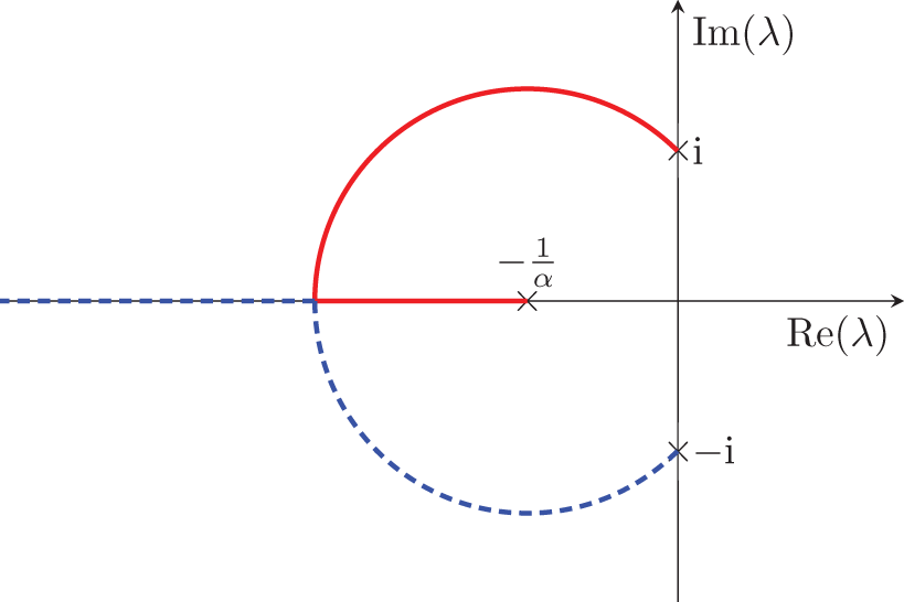


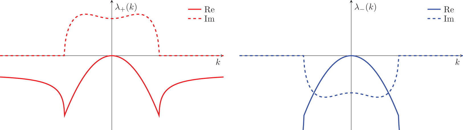


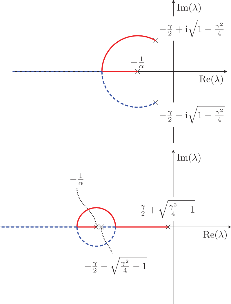


 Open access