


1. Introduction
Due to their importance in numerous engineering and natural systems, the scaling of turbulent wall-bounded flows has been a subject of great interest (e.g. Coles Reference Coles1956; Smits et al. Reference Smits, Monty, Hultmark, Bailey, Hutchins and Marusic2011; Marusic et al. Reference Marusic, Monty, Hultmark and Smits2013). Close to the wall, the mean flow follows inner scaling, with a characteristic velocity scale called the friction velocity,  $u_\tau =(\tau _w/\rho )^{-1/2}$, and a characteristic length scale called the viscous length scale, $\nu /u_\tau$, where $\tau _w$ is the wall shear stress, and $\rho$ and $\nu$ are the density and kinematic viscosity of the fluid, respectively. In the outer part of the flow, the statistics follow outer scaling, with the same velocity scale $u_\tau$ but a different length scale corresponding to the layer thickness $\delta$. At high Reynolds numbers, an overlap region develops where both scalings are valid. These observations hold for pipe, channel and boundary layer flows, but the external boundary conditions produce some differences in the functional relationships among these flows in the outer region (that is, in the wake region).
The turbulent stresses generally follow this scaling behaviour, except that the large-scale motions in the outer and overlap regions interact with the small-scale motions in the inner region through time-dependent superimposition and amplitude modulation, so the amplitudes of the inner layer stresses display a Reynolds number dependence (e.g. Mathis, Hutchins & Marusic Reference Mathis, Hutchins and Marusic2009; Marusic, Mathis & Hutchins Reference Marusic, Mathis and Hutchins2010; Smits Reference Smits2020; Smits et al. Reference Smits, Hultmark, Lee, Pirozzoli and Wu2021). Nevertheless, the stresses all display a wide range of wavenumbers, and Kolmogorov (Reference Kolmogorov1941) proposed that at sufficiently large Reynolds number, the small scales of turbulence (the high wavenumber parts of the spectrum) are homogeneous and isotropic, and independent of boundary conditions, thereby having universal characteristics dictated only by the mean dissipation rate  $\langle \varepsilon \rangle$ of turbulent kinetic energy, and $\nu$. We use $\langle \cdot \rangle$ to indicate a mean quantity assessed over a statistically homogeneous ensemble. For the stationary and ergodic flows considered here, we determine $\langle \cdot \rangle$ using a time average that is thus dependent on spatial position. There is an intermediate range of wavenumbers, called the inertial subrange, where the power spectral density is independent of the viscosity and follows the famous $-5/3$ law. At the highest wavenumbers, in the dissipative range where viscosity is dominant, dimensional analysis of $\langle \varepsilon \rangle$ and $\nu$ yields the Kolmogorov length scale $\langle \eta _K \rangle =(\nu ^3/\langle \varepsilon \rangle )^{1/4}$ and velocity scale $u_\eta =(\langle \varepsilon \rangle \nu )^{1/4}$. Kolmogorov scaling has been tested extensively in wall-bounded flows (e.g. Saddoughi & Veeravalli Reference Saddoughi and Veeravalli1994) and found to successfully scale the dissipative motions, for example through the collapse of the high-wavenumber end of energy spectra scaled by $\langle \varepsilon \rangle$, $\nu$ and $\langle \eta _K \rangle$ (e.g. Grant, Stewart & Moilliet Reference Grant, Stewart and Moilliet1962; Rosenberg et al. Reference Rosenberg, Hultmark, Vallikivi, Bailey and Smits2013).
What has received less attention in wall-bounded flow is the wavenumber relationship between inner/outer scales,  $\delta$ and $\nu /u_\tau$, and their commensurate scales $\mathcal {L}$ and $\langle \eta _K \rangle$, where $\mathcal {L}$ is a characteristic measure of the low-wavenumber end of the spectrum (e.g. Kolmogorov Reference Kolmogorov1941; Pope Reference Pope2000). Of interest here is the universality of this coupling among internal (pipe and channel) and external (turbulent boundary layer) flows. One of the challenges associated with our investigation is that the Reynolds number needs to be large enough to achieve sufficient separation of scales, so that $\delta \gg u_\tau /\nu$ and $\mathcal {L} \gg \langle \eta _K \rangle$.
Complicating any comparison between internal and external flows is the presence of intermittency in external flows, where laminar freestream fluid is entrained into the boundary layer along a time-dependent turbulent/non-turbulent interface (Kovasznay, Kibens & Blackwelder Reference Kovasznay, Kibens and Blackwelder1970). This interaction between turbulent and non-turbulent fluid, which is absent in fully-developed channel and pipe flows, occurs on two separate scales: one that is correlated with the size of the large-scale motions in the outer layer ( $\sim 2\delta$– $3\delta$), and one that is a diffusive, viscous scale at the interface itself (Kovasznay Reference Kovasznay1967). The first is called the entrainment scale, and the second is referred to as nibbling at the interface (Mathew & Basu Reference Mathew and Basu2002; Westerweel et al. Reference Westerweel, Fukushima, Pedersen and Hunt2005; Holzner et al. Reference Holzner, Liberzon, Nikitin, Kinzelbach and Tsinober2007). The level of intermittency varies strongly with the distance from the wall; near the wall, the flow is fully turbulent, while it is laminar in the freestream. Hence it can be expected that the presence of intermittency provides a strong influence on any locally averaged statistics calculated in the outer layer of external flows.
Here, we combine previously unpublished highly resolved experimental data from a high-Reynolds-number turbulent boundary layer with previously published well-resolved high-Reynolds-number pipe and boundary layer measurement data to examine the relationship between different length scales of turbulence, with particular focus on the influence of external intermittency on the comparison between internal to external flows. The high Reynolds numbers of these data allows the conditions required for the formation of an inertial subrange, i.e.  $\mathcal {L} \gg \langle \eta _K \rangle$, to be met. With these data, we show that properly selected small-scale turbulence descriptors follow inner scaling throughout the wall-bounded flow, including in regions expected to be described by outer scaling, and that properly selected descriptors of large-scale turbulence follow outer scaling throughout the wall-bounded flow. Similar behaviour was observed for both internal and external boundary layer flows, once rectification had been applied for the effects of external intermittency, and we show that these scales can be related to features in the longitudinal energy spectrum.
2. Experiments description
2.1. Facilities and flow conditions
The high-Reynolds-number wall-bounded flow data were acquired using thermal anemometry in three different facilities. Two data sets come from compressed-air facilities: the High Reynolds Number Test Facility (HRTF) at the Princeton University Gas Dynamics Lab, in which a zero-pressure-gradient turbulent boundary layer was developed along a smooth flat plate in a compressed-air wind tunnel (with the measurements described in Vallikivi, Hultmark & Smits Reference Vallikivi, Hultmark and Smits2015b); and the canonical pipe flow produced by the Superpipe facility at the Princeton University Gas Dynamics Lab (with the measurements described in Hultmark et al. Reference Hultmark, Vallikivi, Bailey and Smits2012, Reference Hultmark, Vallikivi, Bailey and Smits2013). These data are complemented by additional, previously unpublished measurements taken in the High Reynolds Number Boundary Layer Wind Tunnel (HRNBLWT) at the University of Melbourne, Australia, in which the turbulent boundary layer develops along the wind tunnel floor. The HRNBLWT facility is described in Nickels et al. (Reference Nickels, Marusic, Hafez, Hutchins and Chong2007).
Experimental conditions are summarized in tables 1–3 for the HRNBLWT, HRTF and Superpipe, respectively. In this study,  $\delta$ represents the radius and 99 % boundary layer thickness for the pipe and turbulent boundary layer cases, respectively. Note that for the HRNBLWT turbulent boundary layer data, the friction velocity was estimated using the Clauser approach using von Kármán constant 0.39, whereas for the HRTF data, multiple techniques were used to estimate $u_\tau$ (see Vallikivi et al. Reference Vallikivi, Hultmark and Smits2015b). For the Superpipe measurements, the friction velocity was determined from the pressure loss measured along a length of the pipe (Hultmark et al. Reference Hultmark, Vallikivi, Bailey and Smits2013). It should be noted that some differences have been observed between the mean velocity profiles of the corrected Pitot data and those produced by the Hultmark et al. (Reference Hultmark, Vallikivi, Bailey and Smits2013) data, which may be due to uncertainty in the determined friction velocity (e.g. Bailey et al. Reference Bailey, Vallikivi, Hultmark and Smits2014). The data set encompasses an order of magnitude of Reynolds number range $2000\lesssim Re_\tau \lesssim 38\,000$ in pipe flow, and $2500\lesssim Re_\tau \lesssim 17\,000$ for the turbulent boundary layer. The HRNBLWT measurements, having higher resolution than the HRTF measurements, also provide confidence that observations made are agnostic to both facility and sensor resolution.
Table of experimental conditions, HRNBLWT.

Table of experimental conditions, HRTF.

Table of experimental conditions, Superpipe.

2.2. Instrumentation
To achieve the spatial and temporal resolutions required to resolve near-Kolmogorov scales at these Reynolds numbers, a nanoscale thermal anemometry probe (NSTAP) was used for all cases (as described in Bailey et al. Reference Bailey, Kunkel, Hultmark, Vallikivi, Hill, Meyer, Tsay, Arnold and Smits2010; Vallikivi et al. Reference Vallikivi, Hultmark, Bailey and Smits2011; Hultmark et al. Reference Hultmark, Vallikivi, Bailey and Smits2012, Reference Hultmark, Vallikivi, Bailey and Smits2013; Vallikivi & Smits Reference Vallikivi and Smits2014; Bailey & Witte Reference Bailey and Witte2016). These probes measured the streamwise,  $U_1$, component of velocity. Here, we will use subscripts $1,2,3$ to indicate streamwise, wall-normal and transverse directions, respectively.
The probe used in these experiments had a sensing element measuring  $\ell =60\ \mathrm {\mu }$m long by 2 $\mathrm {\mu }$m wide by 100 nm thick. The resulting $\ell ^+$ values are provided in tables 1–3 for each case. Noting that the minimum $\langle \eta _K \rangle ^+$ is 2–3, these $\ell ^+$ values indicate that the probes were smaller than the Kolmogorov scale for all HRNBLWT cases, and for $Re_\tau <5000$ for the Superpipe cases. At the highest $Re_\tau$ measured, the probe was only at the same order of magnitude of $\langle \eta _K \rangle$ within the outer layer. In addition, Monkewitz (Reference Monkewitz2022) noted that sensor blockage could influence statistics measured by the NSTAP when the probe was less than 300 $\mathrm {\mu }$m from the wall. However, comparison of HRNBLWT and HRTF cases at matched $Re_\tau$ suggests that the reduced spatial resolution and increased potential for probe blockage within the compressed-air facilities does not appear to have a significant impact on the statistics considered here.
In all cases, the NSTAP probes were operated using a Dantec Streamline anemometer with resistance overheat ratio 1.2. However, digitization frequencies ranged from 250 kHz for the HRNBLWT cases to 300 kHz for the HRTF and Superpipe cases, with corresponding analogue anti-aliasing low-pass filter frequencies 100 kHz. Calibration of the probes took place in situ, directly prior to, and following, each measurement run using a Pitot-static tube located outside the boundary layer or at the centreline of the pipe. For all cases, measurements were conducted at more than 40 positions in the wall-normal  $y=x_2$ direction.
Due to the feedback circuit employed in constant-temperature anemometry, and sample rates exceeding the energy content of the turbulence, there was  $f^2$ noise (Saddoughi & Veeravalli Reference Saddoughi and Veeravalli1996) present in the data at high frequencies. Therefore, when post-processing the data, we assumed that the frequency at which the local gradient of spectra transitions from negative to positive indicates the point where instrumentation noise is of the same order as turbulent signal (Bailey et al. Reference Bailey, Hultmark, Schumacher, Yakhot and Smits2009). We eliminate frequency content above this point using an eighth-order low-pass digital Butterworth filter with cutoff frequency $f_{cut}$. The actual value of $f_{cut}$ was a function of the signal-to-noise ratio and varied with measurement position, Reynolds number and facility. In all cases, it was determined to be higher than the frequency corresponding to the Kolmogorov time scale.
In addition, Taylor's frozen flow hypothesis was employed to translate temporal statistics into spatial statistics, after ensuring that ratio  $|u_1|/\langle U_1 \rangle$ was sufficiently small (Taylor Reference Taylor1938; Meneveau & Sreenivasan Reference Meneveau and Sreenivasan1991), where $u_1$ arises from Reynolds decomposition following $U_1=\langle U_1\rangle + u_1$. It was thus assumed that local mean velocity is the advective velocity of all turbulent length scales, giving an approximation of spatial separation ${\rm \Delta} x_1 \approx \langle U_1 \rangle \,{\rm \Delta} t$, where ${\rm \Delta} t$ is a time displacement. Generally, Taylor's frozen flow hypothesis provides a reasonable approximation for small scales of turbulence; however, it is understood that it introduces error in translating large scales (Zaman & Hussain Reference Zaman and Hussain1981; del Álamo & Jiménez Reference del Álamo and Jiménez2009).
2.3. External intermittency detection
Appearance of intermittent laminar regions interspersed with regions of turbulent flow is known to bias the probability density functions (PDFs) of local dissipative length scale  $\eta$ towards larger scales within the outer layer (Alhamdi & Bailey Reference Alhamdi and Bailey2018), and a similar influence can be expected on other statistical quantities. Hence an external intermittency detection approach was used to distinguish instances when the probe was within turbulent flow from when it was in laminar flow. In previous work, identification of the turbulent–laminar interface within velocity time series was conducted using detection functions based on time derivatives of velocity components, instantaneous shear stress, velocity magnitude and local kinetic energy (Hedleyt & Keffer Reference Hedleyt and Keffer1974; Tsuji et al. Reference Tsuji, Honda, Nakamura and Sato1991; Chauhan et al. Reference Chauhan, Philip, De Silva, Hutchins and Marusic2014). Here, the kinetic energy criterion was used to identify turbulent regions following the procedure developed by Chauhan et al. (Reference Chauhan, Philip, De Silva, Hutchins and Marusic2014). This approach assumes that within the outer region of a turbulent boundary layer, non-turbulent regions have an advective velocity close to the external flow velocity $U_{ex}$, while turbulent regions originating from the wall will have mean velocity that is lower than $U_{ex}$ (Corrsin & Kistler Reference Corrsin and Kistler1955; Fiedler & Head Reference Fiedler and Head1966; Kovasznay et al. Reference Kovasznay, Kibens and Blackwelder1970; Jiménez et al. Reference Jiménez, Hoyas, Simens and Mizuno2010; Chauhan et al. Reference Chauhan, Philip, De Silva, Hutchins and Marusic2014). This allows the formation of the detection function
 \begin{equation} \gamma(t)=100\left(1-\frac{U_1(t)}{U_{ex}}\right)^2,\end{equation}
such that, when combined with a threshold value, the region is assumed to be non-turbulent when  $\gamma (t)$ is less than the threshold. Previous experimental work showed that in case of the external boundary layer, the freestream turbulence intensity is not exactly zero, in contrast to jet flows, thus selecting correct threshold value can be challenging (Chauhan et al. Reference Chauhan, Philip, De Silva, Hutchins and Marusic2014). Here, the threshold value $\gamma _t=0.05$ was used, which corresponds to $|u_1|\approx 0.02U_{ex}$ at the edge of the boundary layer.
Using this indicator, statistics could be extracted from only the turbulent regions detected within the time series. Note that external intermittency was most evident for  $y/\delta \gtrsim 0.5$, increasing in frequency with $y$, and reaching a maximum frequency at $y\approx 0.7\delta$. For $y>0.8\delta$, external laminar flow was predominant, which meant that the average length of laminar regions became larger than the average length of turbulent regions. Hence as $y$ approached $\delta$, some individual turbulent regions were found to become too short to achieve converged statistics. To address this issue, the minimum size of turbulent regions considered was set at half the boundary layer thickness. This value ( $\gtrsim 0.5\delta$) was selected for two reasons: (1) it was found to be the minimum value that allowed calculation of acceptable energy spectra; and (2) it ensured that the lengths of the shortest turbulent regions were of the order of the wall-normal distance and/or the boundary layer thickness. For the purpose of the current paper, small-scale nibbling motions around the interface were assumed to be a part of the turbulent structure, therefore only larger-scale motions ( $\approx {O}(\delta )$, as suggested by Chauhan et al. Reference Chauhan, Philip, De Silva, Hutchins and Marusic2014) were considered in separating turbulent/non-turbulent flows. However, it was found that effects of including short regions in deriving the statistics were insignificant for the range $0.5\delta \lesssim y \lesssim \delta$.
Finally, when calculating point statistics requiring an advective velocity, the advective velocity used was the global mean value of all the turbulent regions. This was done to account for contributions to the local fluctuations from the different advective velocities of each turbulent region. Conversely, to avoid biases by the interfaces when calculating time-dependent statistics, these were calculated using the advective velocity for the individual turbulent regions and then ensemble averaged. For example, to evaluate the energy spectrum at a wall-normal distance within the region influenced by external intermittency, the spectrum was calculated for each portion of the time series identified as turbulent, and then interpolated to a common wavenumber vector prior to averaging.
3. Results
3.1. Large scales
We begin by examining the scaling of parameters used to characterize large and most energetic scales of turbulence,  $\mathcal {L}$. In practice, the integral length scale ${ILS}$ is often used as a measure of $\mathcal {L}$, to represent the low wavenumber end of the inertial subrange (or the beginning of the $-5/3$ region). To calculate ${ILS}$, we used Taylor's hypothesis and integrated the autocorrelation following
 \begin{equation} {ILS}=\frac{\langle U_1 \rangle}{\langle u_1^2 \rangle}\int_0^{\tau_c}\langle u_1(t+\tau)u_1(t)\rangle \, {\rm d} \tau, \end{equation}
where  $\tau _c$ is the value of $\tau$ where the autocorrelation first reaches value 0.
Wall-bounded turbulent flow has large-scale anisotropic structures that will influence  ${ILS}$, which here is calculated using the longitudinal velocity component only. These structures include sublayer streaks (Kline et al. Reference Kline, Reynolds, Schraub and Runstadler1967), hairpin vortices near the wall (Head & Bandyopadhyay Reference Head and Bandyopadhyay1981), large-scale motions corresponding to bulges of turbulence at the edge of the wall layer (Kim & Adrian Reference Kim and Adrian1999; Guala, Hommema & Adrian Reference Guala, Hommema and Adrian2006; Balakumar & Adrian Reference Balakumar and Adrian2007), and superstructures of very large scale within the overlap region and, in the case of pipe and channel flows, within the wake region as well (Kim & Adrian Reference Kim and Adrian1999; Hutchins, Hambleton & Marusic Reference Hutchins, Hambleton and Marusic2005; Monty Reference Monty2005; Tomkins & Adrian Reference Tomkins and Adrian2005; Guala et al. Reference Guala, Hommema and Adrian2006; Balakumar & Adrian Reference Balakumar and Adrian2007; Monty et al. Reference Monty, Hutchins, Ng, Marusic and Chong2009). Large-scale motions also modulate the near-wall flow and influence the flow structure near the wall (Mathis et al. Reference Mathis, Hutchins and Marusic2009). Considering the various length scales of these energy-containing motions, the ${ILS}$ value can be expected to represent a superposition of a range of anisotropic contributions, and therefore may not be an appropriate metric to exemplify the idealized isotropic eddies below the low-wavenumber end of the inertial subrange. Within wall bounded flows, it has also been suggested that the energy-containing range of the spectrum depends on $\delta$, with an overlap inertial layer scaling with $y$ (Perry, Henbest & Chong Reference Perry, Henbest and Chong1986; Morrison et al. Reference Morrison, McKeon, Jiang and Smits2004; Vallikivi, Ganapathisubramani & Smits Reference Vallikivi, Ganapathisubramani and Smits2015a).
An alternative approach to describe  $\mathcal {L}$, which can be used when there is no clear geometric large scale, can be found from scaling arguments based on the energy cascade, specifically
 \begin{equation} \mathcal{L} = \frac{{TKE}^{3/2}}{\langle \varepsilon \rangle},\end{equation}
where  ${TKE}$ is the turbulent kinetic energy.
However, (3.2) requires estimation of both mean dissipation rate  $\langle \varepsilon \rangle$ and turbulent kinetic energy ${TKE}$. As the NSTAP was unable to resolve more than one component of velocity, we instead use the approximation
 \begin{equation} L\approx\frac{ \left(\frac{3}{2}\langle u_1^2 \rangle \right)^{3/2}}{\langle \varepsilon \rangle}. \end{equation}
Note that due to the anisotropy of wall-bounded turbulence,  $\frac 32 \langle u_1^2 \rangle$ should not be considered to be an accurate estimate of $TKE$. Furthermore, $\langle u_1^2 \rangle$ is itself subject to contributions from longitudinal energetic structures, hence their contribution cannot be neglected, and $L$ should be considered as an estimate of the longitudinal scale of the large eddies. When examining the scaling of dissipative motions at low $Re_\tau$ (Alhamdi & Bailey Reference Alhamdi and Bailey2017, Reference Alhamdi and Bailey2018), this measure of the longitudinal length scale provided reasonable scaling of fine turbulent structure within the boundary layer for the entire range of $y$, once external intermittency was accounted for.
The mean dissipation rate  $\langle \varepsilon \rangle$ was found assuming local isotropy and integrating the one-dimensional dissipation spectrum $D(k_1)$ (Townsend Reference Townsend1976). This, in turn, was approximated by the one-dimensional longitudinal energy spectrum $E_{11}(k_1)$ such that
 \begin{equation} \langle \varepsilon \rangle \approx \int_0^{k_c} D(k_1) \, {\rm d} k_1 \approx 15\nu \int_0^{k_c} k_1^2\, E_{11}(k_1) \, {\rm d} k_1, \end{equation}
where the streamwise wavenumber was found from frequency  $f$ according to $k_1\approx 2{\rm \pi} f/\langle U_1\rangle$. Note that $k_c$ is the wavenumber representation of the filter frequency $f_{cut}$. For $y^+>50$, comparison of $\langle \varepsilon \rangle$ calculated using this approach by Bailey & Witte (Reference Bailey and Witte2016) in channel flow was found to compare favourably to the $\langle \varepsilon \rangle$ values calculated from the direct numerical simulation data of Lee & Moser (Reference Lee and Moser2015) at similar Reynolds numbers. The reduced agreement for $y^+<50$ can be attributed to the reduced scale separation and increased anisotropy of the small scales near the wall. Similar behaviour can be expected in the current data set.
It was found that the HRTF data had under-resolved high-frequency content due to low signal-to-noise ratio at the high frequency. Therefore, to obtain estimates of  $\langle \varepsilon \rangle$ for these cases, the longitudinal energy spectrum scaling was assumed, allowing a fit to the inertial subrange such that
 \begin{equation} \langle \varepsilon \rangle\approx\left(\frac{1}{C_1}\,k_1^{5/3}\, E_{11}(k_1)\right)^{3/2}, \end{equation}
using  $C_1=0.53$ as suggested by Sreenivasan (Reference Sreenivasan1995).
Although both  ${ILS}$ and $L$ have been identified as potential characteristic longitudinal length scales of the energy containing eddies, which are expected to scale with $\delta$, comparison of the outer-scaled behaviour between the two, as done in figure 1, shows significant differences in their scaling behaviours. Figure 1(a) reveals that despite there being collapse of ${ILS}/\delta$ for $y/\delta <0.05$, for $y/\delta >0.05$ there is both Reynolds-number-dependent and geometry-dependent variability observed. Although ${ILS}\approx \delta$ for $y/\delta >0.1$, the profiles of $L/\delta$ shown in figure 1(b) show larger values with $L\approx 1.5\delta$–2.5 $\delta$. Hence, with increasing $y$, the values of $L$ are larger than ${ILS}$ for $y/\delta >0.5$, although neither appears to capture the scale of large-scale (2 $\delta$–3 $\delta$) or very-large-scale (10 $\delta$–20 $\delta$) motions.
Outer-scaled (a)  ${ILS}$ and (b) $L$, including laminar portions of the time series in the ${ILS}$ and $L$ calculation. Corresponding outer-scaled profiles using only turbulent portions of the time series in the calculation are shown in (c) ${ILS}$ and (d) $L$. All cases are shown with symbols as provided in tables 1–3.

For both  ${ILS}/\delta$ and $L/\delta$, the boundary layer cases show higher Reynolds number dependence than the pipe flow cases for all $y<\delta$. Notably, this behaviour changes significantly when only the turbulent regions of the outer layer are considered when calculating these scales, as shown in figures 1(c) and 1(d) for ${ILS}/\delta$ and $L/\delta$, respectively. From figure 1(c), it is evident that the Reynolds number dependence of ${ILS}/\delta$ for the boundary layer is reduced significantly, and two clear trends appear, differentiating the pipe and boundary layer flow behaviours. The decrease in ${ILS}/\delta$ evident with increasing $y/\delta$ is consistent with the wall-normal structure of the uniform momentum zones observed in turbulent boundary layers (de Silva, Hutchins & Marusic Reference de Silva, Hutchins and Marusic2016).
Interestingly, as shown in figure 1(d), there is an increased agreement between pipe and boundary layer cases in the wall-normal dependence of  $L/\delta$ (in the range $0.05< y\leq \delta$) once the boundary layer cases have been corrected for external intermittency. Note that variability in the $L/\delta$ scaling for $y/\delta <0.05$ could be attributed to the approximations used to estimate $\langle \varepsilon \rangle$. The improvement in agreement further from the wall suggests that much of the differences between the two geometries in the outer layer can be attributed to external intermittency. One possible explanation for this reduced geometry dependence is that $L$, being composed of $\langle u_1^2 \rangle$ and $\langle \varepsilon \rangle$, will be modulated by the isotropy of $\langle \varepsilon \rangle$, and much more tightly bounded by $y$ than ${ILS}$ which, as discussed previously, can include increased contributions from anisotropic large scales.
This last observation is further highlighted by comparing the  ${ILS}/\langle \eta _K \rangle$ and $L/\langle \eta _K \rangle$ Reynolds number dependence which, following classical scaling arguments, is expected to follow $Re_{{ILS}}^{3/4}$ or $Re_L^{3/4}$ behaviour, respectively. Here, $Re_{{ILS}}=\langle | \varDelta _{{ILS}}| \rangle \,{ILS}/\nu$ and $Re_{L}=\langle | \varDelta _{L}| \rangle \,L/\nu$, where
 \begin{equation} \varDelta_\tau =u_1(t+\tau)-u_1(t),\end{equation}
is the longitudinal velocity increment, and  $|\tau |$ is equal to ${ILS}/\langle U_1 \rangle$ and $L/\langle U_1 \rangle$ for $\varDelta _{{ILS}}$ and $\varDelta _L$, respectively.
In figures 2(a,b), we compare the scaling of  ${ILS}/\langle \eta _K \rangle$ as a function of $Re_{{ILS}}$ to the scaling of $L/\langle \eta _K \rangle$ as a function of $Re_L$. Although both descriptions of the large scales produce trends close to the expected ${3/4}$ exponent, the ${ILS}/\langle \eta _K \rangle$ scaling shows more variability about the slope. Although it is not strictly clear in figure 2(a), at high $Re_{{ILS}}$ a single profile can produce multiple values of ${ILS}/\langle \eta _K \rangle$ for the same value of $Re_{{ILS}}$. This is best illustrated in figure 2(c), which isolates the single case of pipe flow at $Re_\tau =10\,500$.
Scale separation represented by (a)  ${ILS}/\langle \eta _K \rangle$ and (b) $L/\langle \eta _K \rangle$ as functions of $Re_{{ILS}}$ and $Re_L$, respectively. The same results isolated for a single case of pipe flow at $Re_\tau =10\,500$ are shown in (c) and (d), respectively. Symbols as provided in tables 1–3, with a red line indicating $Re_{{ILS}}^{3/4}$ in (a), and $Re_{L}^{3/4}$ in (b). External intermittency effects are accounted for in both (a) and (b).

Conversely,  $L/\langle \eta _K \rangle$ (see figure 2b) has much more consistent agreement with the theoretical $3/4$ slope, and little evidence of non-uniqueness in the $Re_L$ dependence. Figure 2(d) shows this behaviour for the isolated pipe flow case at $Re_\tau =10\,500$. However, for $Re_L>10^3$, the local slope of $L/\langle \eta _K \rangle$ deviates from $Re_L^{3/4}$ and becomes closer to $Re_L^{0.76}$. Note that the agreement of the $L/\langle \eta _K \rangle$ scaling is not unexpected as $\langle \eta _K \rangle \sim L\,Re_L^{-3/4}$ can be recovered exactly by replacing $\varDelta _L$ with $\langle u_1^2 \rangle ^{1/2}$ as the velocity scale in $Re_L$. Therefore, the deviation from $3/4$ slope in figure 2(b) reflects the difference between $\langle u_1^2 \rangle ^{1/2}$ and $\varDelta _L$ as representative velocity scales associated with $L$. However, since $\langle u_1^2 \rangle ^{1/2}$ is an integrated quantity over all scales, it is less descriptive of the largest scales, therefore it makes heuristic sense to use $\varDelta _L$ as a description of the large-scale turbulence as it is linked directly to the energy at spatial scale $L$. There is also deviation of $L/\langle \eta _K \rangle$ from $3/4$ slope at $Re_L<200$, which can be attributed to insufficient scale separation.
To summarize, the comparison of  ${ILS}$ to $L$ as a characteristic measure of the longitudinal large length scale of wall-bounded turbulent flow demonstrates that $L$ exhibits significantly less dependence on $Re_\tau$ and geometry. There are two potential reasons for this result. First, in fixed-point measurements, calculation of ${ILS}$ requires assuming that Taylor's frozen flow hypothesis is valid at large scales. It has long been acknowledged that Taylor's hypothesis can bias large-scale statistics (e.g. del Álamo & Jiménez Reference del Álamo and Jiménez2009). Conversely, the calculation of $L$ requires the Taylor's hypothesis to be valid only at small scales, which is a more reasonable assumption, at least farther from the wall ( $y^+>50$). Second, since ${ILS}$ is a superposition of a wide range of large length scales, it is influenced by external intermittency. Even when a correction is imposed (e.g. (2.1)), the correction effectively high-pass filters integral statistics by segmenting the turbulent regions into smaller ensembles, which reduces the measured longitudinal scale. In contrast, $L$, being a point statistic (which can also be calculated in the statistically homogeneous spanwise and azimuthal directions), displays greatly reduced $Re_\tau$ and geometry dependence once external intermittency corrections have been applied.
3.2. Small scales
We now examine the effect of external intermittency on the scaling of the smallest, dissipative motions of turbulence. To do so, we examine not just the scaling of the Kolmogorov scale  $\langle \eta _K \rangle$, but also an alternative descriptor $\eta _0$, introduced to account for internal intermittency (Yakhot Reference Yakhot2006; Hamlington et al. Reference Hamlington, Krasnov, Boeck and Schumacher2012a; Schumacher et al. Reference Schumacher, Scheel, Krasnov, Donzis, Yakhot and Sreenivasan2014). This length scale, defined as $\eta _0\sim L\, Re_L^{-0.73}$, can be considered as analogous to $\langle \eta _K \rangle$, but intrinsically enforces the scaling presented in figure 2. We first examine the inner-scaled behaviour of these parameters using figure 3, which shows $\langle \eta _K\rangle ^+ =\langle \eta _K \rangle u_\tau /\nu$ and $\eta _0^+=\eta _0 u_\tau /\nu$ as functions of inner-scaled wall-normal distance $y^+=y u_\tau /\nu$.
Inner-scaled (a)  $\langle \eta _K \rangle$ and (b) $\eta _0$, including laminar portions of the time series in the $\langle \eta _K \rangle$ and $\eta _0$ calculations. Corresponding inner-scaled profiles using only turbulent portions of the time series in the calculation are shown in (c) $\langle \eta _K \rangle$ and (d) $\eta _0$. All cases are shown with symbols as provided in tables 1–3. Blue lines indicate (3.7), and red lines indicate (3.8).

The quantities  $\langle \eta _K \rangle$ and $\eta _0$ represent two approaches to quantify the dissipative scales, and as shown in figures 3(a,b), both of these metrics for the small scales exhibit inner scaling in the near-wall region for both geometries over a wide range of Reynolds numbers, with $\langle \eta _K \rangle ^+$ exhibiting better agreement than $\eta _0^+$. Notably, the pipe flow results exhibit collapse over the entire range of $y^+$ values, whereas the turbulent boundary layer results exhibit $Re_\tau$ dependence in the outer layer. This last observation is shown to be a consequence of external intermittency as demonstrated by figures 3(c,d), which reveals that once external intermittency was accounted for, both parameters scale well using inner scaling over the entire depth of the wall-bounded flow over a large Reynolds number range and independent of boundary conditions. That said, figure 3(c) does show some residual outer-layer dependence, with deviations from the general trend less than 20 %. Similar outer-layer dependence was noted in the lower-Reynolds-number channel flow measurements of Bailey & Witte (Reference Bailey and Witte2016).
Note that  $\langle \eta _K \rangle ^+$ and $\eta _0^+$ are of the same order, and both show dependence on $y^+$, which can be expected given the change in local turbulence Reynolds number and corresponding wall-distance-dependent scale separation within the turbulence. However, a slightly different relationship with $y^+$ can be observed between the two, as could be expected from the different $Re_L$ behaviours for these two parameters.
For  $y^+\geq 10$, the wall-normal dependencies of both $\langle \eta _K \rangle ^+$ and $\eta _0^+$ were well represented by empirical power-law approximations
 \begin{equation} \langle \eta_K \rangle ^+\approx 0.85 (y^+)^{0.25} \coth{\left(\frac{y^+}{50}\right)}^{0.3}\end{equation}
and
 \begin{equation} \eta_0^+\approx 1.45 (y^+)^{0.23} \coth{\left(\frac{y^+}{20}\right)}^{0.25},\end{equation}
where the hyperbolic cotangent is introduced as a damping function to represent the increased influence of viscosity near the wall (see figure 3).
Both dissipation rate and scales have also been understood to have spatially intermittent behaviour, where regions of intensive dissipation are separated by regions of lower turbulent dissipation rate (Batchelor & Townsend Reference Batchelor and Townsend1949). This internal intermittency suggests that the mean dissipation rate, and by extension  $\langle \eta _K \rangle$, may be a poor representation of the highly skewed dissipation field (Schumacher et al. Reference Schumacher, Scheel, Krasnov, Donzis, Yakhot and Sreenivasan2014). Instead, it has been proposed that treating dissipation as a random fluctuating field introduces the potential for improved scaling of small-scale statistics at higher-order moments (Yakhot Reference Yakhot2006; Yakhot, Bailey & Smits Reference Yakhot, Bailey and Smits2010).
By treating the dissipation scale as a fluctuating field of local dissipation scales, it is then characterized using a distribution of dissipative scales. This distribution can be obtained for the Kolmogorov scales by utilizing the intermittent distribution of dissipation rate. Time series of instantaneous dissipation rate can be approximated using
 \begin{equation} \varepsilon(t)\approx\frac{15\nu}{\langle U_1 \rangle^{2}}\left(\frac{{\rm d} u_1}{{\rm d} t}\right)^2.\end{equation}
In turn, the time dependence of the local Kolmogorov scale can be formed from
 \begin{equation} \eta_K(t)\approx\left(\frac{\nu^3}{\varepsilon(t)}\right)^{1/4},\end{equation}
allowing a probability density function (PDF) of  $\eta _K(t)$ to be calculated from each measured time series.
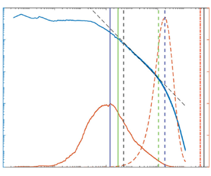
The resulting PDFs  $Q(\eta _K/\langle \eta _K \rangle )$ are presented in figure 4(a) for all data sets considered here, including all $Re_\tau$ and wall-normal distances, totaling 552 time series.
PDFs of (a)  $\eta _K$ and (b) $\eta$ shown normalized, including laminar portions of the time series. Corresponding PDFs considering only turbulent portions of the time series are shown for (c) $\eta _K$ and (d) $\eta$. All measurement locations for all cases measured are shown. The solid blue line is a log-normal distribution with mean $0.28\langle \eta _K \rangle$ and standard deviation $0.45\langle \eta _K \rangle$. The solid red line shows the empirical fit given by (3.12).

The PDFs shown in figure 4(a) are analogous to the moments of the dissipation rate  $\varepsilon ^n/\langle \varepsilon \rangle ^n$ presented in Hamlington et al. (Reference Hamlington, Krasnov, Boeck and Schumacher2012a,Reference Hamlington, Krasnov, Boeck and Schumacherb) and Schumacher et al. (Reference Schumacher, Scheel, Krasnov, Donzis, Yakhot and Sreenivasan2014), who observed universality in the $Re$ dependence of these moments for homogeneous isotropic turbulence, the centreline of turbulent channel flow and the centre of Rayleigh–Bénard convection cells – locations where mean shear is minimal. However, they also observed that mean shear affects the PDF of local dissipation scales at low $Re$. Figure 4(a) shows that although the same general distribution is observed for the different $Re_\tau$ and wall-normal positions (i.e. mean shear) considered here, there is significant variability in the distributions.
Alternative approaches to describing the dissipative scales have also been proposed (Paladin & Vulpiani Reference Paladin and Vulpiani1987). For example, one possibility is to define a local dissipation scale  $\eta$ using the velocity increment (3.6) such that $\varDelta _\tau$ is found with $|\tau |=\eta /\langle U_1 \rangle$ (Yakhot Reference Yakhot2006; Schumacher, Sreenivasan & Yakhot Reference Schumacher, Sreenivasan and Yakhot2007). The definition of a dissipation scale is therefore an event where
 \begin{equation} \eta\,|\varDelta_\eta|\approx\nu.\end{equation}
This is equivalent to identifying instances where the local Reynolds number is of order unity, i.e.  $Re_\eta =\eta \varDelta _\eta /\nu ={O}$(1). When normalized by the scaling parameter $\eta _0$, the PDFs obtained from high-resolution direct numerical simulations data of homogeneous and isotropic turbulence as well as turbulent channel flows (Bailey et al. Reference Bailey, Hultmark, Schumacher, Yakhot and Smits2009; Hamlington et al. Reference Hamlington, Krasnov, Boeck and Schumacher2012a; Bailey & Witte Reference Bailey and Witte2016) were found to be in good agreement. The equivalent PDFs $Q(\eta /\eta _0)$ for the experiments considered here were found following the procedure described in Bailey & Witte (Reference Bailey and Witte2016). Specifically, for each time series, for all $t$,
$t$,  $\varDelta _\tau$ was calculated where the time step $\tau$ was calculated using Taylor's hypothesis as $\tau =\eta /\langle U_1 \rangle$. Then instances where $0.5\leq Re_\eta \leq 2$ were identified and counted to obtain a numerical distribution $P(\eta )$ over the range $0<\eta <4L$. The PDFs were then found from $P(\eta )$ by normalization, such that $Q(\eta )=\int _0^{4L}P( \eta )\, {\rm d}\eta =1$.
The resulting PDFs are shown in figure 4(b) and take the form of a highly skewed distribution, with a peak at  $\eta \approx 2\eta _0$, indicating that dissipation can occur at scales much larger than $\eta _0$, including at energy-producing scales. Notably, there is much less scatter in the distributions, although some variability can be observed and attributed to the outer-layer regions of the boundary layer cases. This variability was attributed previously to the presence of external intermittency by Alhamdi & Bailey (Reference Alhamdi and Bailey2018), and when external intermittency is accounted for, as shown in figure 4(d), there is significantly better agreement between all $Re_\tau$, wall-distance and geometries considered here.
Furthermore, when the PDFs  $Q(\eta _K/\langle \eta _K \rangle )$ are also calculated accounting for the presence of external intermittency, the variability in the resulting distributions is also significantly reduced, although there is still some higher-order variability evident. This is illustrated by the distributions in figure 4(c) being well approximated for $\eta _K\approx \langle \eta _K \rangle$ by a log-normal distribution with mean $0.28\langle \eta _K \rangle$ and standard deviation $0.45\langle \eta _K \rangle$. Note that at the tails of $Q(\eta _K/\langle \eta _K \rangle )$, additional noise was evident due to limited instrumental sensitivity for these small velocity differences (i.e. for large values of $\eta _K$, the local dissipation rate $\varepsilon$, and thus velocity difference, must be small).
Clear differences in the distribution of dissipation scales appear between the approaches used in figures 4(c) and figure 4(d). The  $Q(\eta _K/\langle \eta _K \rangle )$ distributions are noticeably less skewed, with much more concentration at smaller scales than the corresponding $Q(\eta /\eta _0)$ distributions. Both approaches demonstrated good collapse of PDFs, with peaks at $\langle \eta _K \rangle$ and $2\eta _0$, respectively, representing a factor of 3 difference in the most probable length scale (as indicated by figure 3).
Furthermore, as noted previously,  $Q(\eta /\eta _0)$ shows good collapse over the entire range of $\eta /\eta _0$, while $Q(\eta _K/\langle \eta _K \rangle )$ has better agreement for the peak of the PDF. Similar observations of universality of these distributions have been made previously, although previous measurements of $Q(\eta /\eta _0)$ were limited to relatively low Reynolds numbers (Bailey et al. Reference Bailey, Hultmark, Schumacher, Yakhot and Smits2009; Zhou & Xia Reference Zhou and Xia2010; Hamlington et al. Reference Hamlington, Krasnov, Boeck and Schumacher2012a; Morshed, Venayagamoorthy & Dasi Reference Morshed, Venayagamoorthy and Dasi2013; Alhamdi & Bailey Reference Alhamdi and Bailey2017).
Finally, it was also found that the structure of  $Q(\eta /\eta _0)$ over the range $1/4\leq \eta /\eta _0\leq 10^4$ could be well approximated by the empirical function
 \begin{equation} Q({\eta}/{\eta_0})\approx\frac{12^{(\eta/\eta_0)^{0.13}} \tanh{(1.3 \eta/\eta_0)}^{15}}{16(\eta/\eta_0)^2},\end{equation}
as shown in figure 4(d). Hence (3.8) and (3.12) can be combined to yield the distribution of dissipative scales over a very large Reynolds number range and over all distances from the wall.
3.3. Additional length scales
The length scales  $\langle \eta _K \rangle$ and $\eta _0$ describe the smallest dynamically important scales of turbulence. However, the majority of turbulent kinetic energy dissipation occurs at scales significantly larger than $\langle \eta _K \rangle$ and $\eta _0$ (as illustrated in figure 4, for example).
In many cases, Taylor's microscale  $\lambda _f$ is often used as a proxy to describe the largest length scale at which viscous forces are relevant. In other words, it is used to describe the high-wavenumber end of the inertial subrange, at which dissipation starts becoming significant. This is consistent with Taylor's microscale being an intermediate length scale ( $\mathcal {L}>\lambda _f>\langle \eta _K \rangle$). Following the comparison of the large- and small-scale descriptors between the external and internal flows, we can also examine the scaling of $\lambda _f$. Here, the longitudinal Taylor's microscale was calculated using the isotropic assumptions required for the current data sets such that
 \begin{equation} \lambda_f\approx\left(\frac{30\nu\langle u_1^2\rangle}{\langle \varepsilon \rangle}\right)^{1/2}. \end{equation}
Due to anisotropy in the Reynolds stresses, this approximation will likely result in an overestimation of the Taylor microscale.
As can be seen in figures 5(a,b),  $\lambda _f$ does not follow either inner or outer scaling, deviating from inner scaling for $y^+>100$, and showing no sign of collapse of the data in outer scaling. This can be attributed to the mixed-scale nature of $\lambda _f$, formed from $\langle u_1^2\rangle$, which broadly follows outer scaling for $y/\delta >0.02$ (Hultmark et al. Reference Hultmark, Vallikivi, Bailey and Smits2013), and $\langle \varepsilon \rangle$, which, as demonstrated by figure 3(c), can be expected to follow inner scaling for most of the range $y<\delta$. Note that following the discussion in the previous subsection, the calculation has already accounted for the effects of external intermittency.


As an alternative to  $\lambda _f$ for describing the length scales at which the majority of turbulent kinetic energy dissipation is occurring, we can instead introduce a length scale $L_\varepsilon$ corresponding to the wavenumber at which the peak of the premultiplied dissipation spectrum occurs, i.e. the wavenumber at which $15 \nu k_1^3 E_{11}(k_1)$ is a maximum. This peak is then $2{\rm \pi} /L_\varepsilon$, and represents the scales with the largest contribution to turbulent dissipation, following (3.4).
As shown in figure 6(a), this scale closely follows inner scaling for a wide range of  $Re_{\tau }$ for all three data sets, and is consistent with the scaling of $\langle \eta _K \rangle ^+$ shown in figure 3(c). For $y^+>50$, where small-scale homogeneous and isotropic assumptions are expected to be valid, $L_\varepsilon$ can be approximated by $L_\varepsilon \approx 31\langle \eta _K \rangle$.


Comparing figures 5(a) and 6(a),  $\lambda _f$ and $L_\varepsilon$ are of the same order of magnitude and almost identical at $y^+\approx 50$. However, as the Reynolds number increases with wall-normal distance, the agreement between the two scales disappears, and $\lambda _f^+$ becomes $Re_\tau$- and $y$-dependent.
To assess the relative importance of viscous forces at  $L_\varepsilon$, it is possible to define a local Reynolds number $Re_{L_\varepsilon }=\varDelta _{L_\varepsilon } {L_\varepsilon }/\nu$, where $\varDelta _{L_\varepsilon }$ is the velocity increment from (3.6) with $|\tau |=L_\varepsilon /\langle U_1 \rangle$. This Reynolds number therefore describes the ratio of inertial forces to viscous forces at scales corresponding to $L_\varepsilon$. Figure 6(b) shows $Re_{L_\varepsilon }$ as a function of $y^+$. Interestingly, $Re_{L_\varepsilon }$ is constant near a value of 100 for both Superpipe and HRNBLWT flows for $y^+>50$ for all $Re_\tau$, with the exception of the two highest Reynolds number HRTF cases, in which the calculation of the dissipation spectrum was found to be more challenging due to the presence of high-frequency noise.
Noting that  $L_\varepsilon$ is the scale where turbulence undergoes the highest rate of dissipation, this suggests that dissipation occurs when viscous effects are 1 % of inertial effects. For $y^+<50$, both pipe and boundary layer profiles follow the same trend, forming a peak for $Re_{L_\varepsilon }\approx 250$ at $y^+\approx 10$. This is believed to be due to the fact that despite the peak production occurring in this $y^+$ range, the local $Re_L$ value is relatively small, and there is insufficient separation of scales, resulting in increased inertial eddies occurring at the dissipation scales.
As the scaling of the large-scale turbulence in the boundary layer was found to be impacted significantly by the presence of external intermittency, it therefore becomes of interest to also examine the wavelength of the external intermittency and evaluate how this wavelength might be related to the underlying large-scale motions.
The intermittency detection approach described in § 2.3 provides a consistent way of detecting turbulent regions and the corresponding interface wavelength ( ${IWL}$), which here is quantified by the average time between leading edges of two near turbulent regions at a fixed $y$ location. This time displacement is then transformed to a spatial wavelength through Taylor's hypothesis. Since the frequency of external intermittency was $y$-dependent, the $y$ location selected for defining ${IWL}$ was the location with the most probable interface location, i.e. the location with the highest frequency of intermittent occurrences. From the current data, this location was identified to be at $y\approx 0.7\delta$, which is close to the most probable interface location suggested by Chauhan et al. (Reference Chauhan, Philip, De Silva, Hutchins and Marusic2014). We thus define ${IWL}$ as the average distance between leading edges of two near turbulent regions at $y\approx 0.7\delta$. Note that since the turbulent detection function (2.1) was low-pass filtered, ${IWL}$ is constrained to $\gtrsim 0.5\delta$, resulting in small-scale nibbling motions being neglected.
It was found that  ${IWL}$ is nearly constant, with values between $2.38\delta$ and $2.49\delta$ detected for all $Re_\tau$ cases of the HRNBLWT and HRTF data sets. This is consistent with the $2\delta$– $3\delta$ scales attributed to outer layer bulges, and these motions being coupled with the boundary layer thickness.
4. Connection between scales and features of the wavenumber spectrum
In the previous section, we examined the wall-normal scaling of several characteristic length scales: outer-scaled parameters  ${ILS}$, $L$ and $IWL$, which depend on $\delta$, describing large-scale flow features; inner-scaled parameters $L_\varepsilon$, $\eta _0$ and $\langle \eta _K \rangle$, which describe the dissipative motions; and intermediate length scale $\lambda _f$. In this section, we examine these scales in the wavenumber domain, and examine their relationship to commonly observed spectral features – specifically, the most energetic motions and the inertial subrange boundaries.
Figure 7 presents three different wavenumber spectrum representations: one-dimensional longitudinal energy spectrum  $E_{11}(k_1\langle \eta _K \rangle )$, premultiplied longitudinal energy spectrum $k_1 E_{11}(k_1\langle \eta _K \rangle )$, and the premultiplied dissipation spectrum approximation of $15 \nu k_1^3 E_{11} (k_1\langle \eta _K \rangle )$. These spectra are examined for four wall-normal distances (i.e. different $Re_L$) from the $Re_\tau =9500$ measurements taken in the HRNBLWT turbulent boundary layer. Note that the other cases showed similar results.
Example longitudinal one-dimensional energy spectra ( $E_{11}$), premultiplied longitudinal one-dimensional energy spectra ( $k_1 E_{11}$), and estimated premultiplied dissipation spectra ( $15 \nu k_1^3 E_{11}$). Results are shown for HRNBLWT data taken at $Re_\tau =9500$ for four different wall-normal locations: (a) $y^+=4580$, $y/\delta \approx 0.46$; (b) $y^+=1006$, $y/\delta \approx 0.1$; (c) $y^+=95$, $y/\delta \approx 0.01$; and (d) $y^+=10$, $y/\delta \approx 0.001$. Vertical lines indicate wavenumbers corresponding to scales indicated in the legend.

Interestingly, in the region where external intermittency is prominent (figure 7a), the average spectrum calculated from individual spectra measured in discrete turbulent regions displays a clearly identifiable, well-developed inertial subrange  $E_{11}\propto k_1^{-5/3}$. This is consistent with the scale separation ( $L \gg \langle \eta _K \rangle$ is approximately 3–4 orders of magnitude). The inertial subrange is bounded by $L\approx {IWL}$ at its low-wavenumber end, and by $\lambda _f$ at its high-wavenumber end. In contrast to $L$ and ${IWL}$, ${ILS}$ lies in the inertial subrange and does not correspond to any clearly identifiable spectral feature. As expected, $L_\varepsilon$ is smaller than $\lambda _f$, with the latter being a good representation of the upper bound of the inertial subrange. Hence despite being an average formed from intermittent turbulent regions, this longitudinal energy spectrum exhibits classical high-Reynolds-number energy spectrum characteristics. The exception is at the low-wavenumber end of the spectrum, which is under-resolved due to the variable lengths of the turbulent regions acting as a high-pass filter during the averaging process. Thus the shorter lengths of the turbulent regions do not contain any low-wavenumber information, consistent with its dependence on ${IWL}$.
At measurement locations closer to the wall, where external intermittency is not present, the energy-containing range is extended due to the ability to resolve much longer wavelengths (see figures 7b–d). However, the peak in the energy-containing range still corresponds closely to the scales associated with  ${IWL}$.
Additionally, it was found that  ${IWL}$ is a good approximation of the wavelength associated with the peak of the premultiplied energy spectrum $E_{11}k_1$ for $y^+>200$, as can be seen in figures 7(a,b). Closer to wall, the effect of the turbulent/non-turbulent interface disappears due to the increased importance of viscous forces.
At  $y^+\approx 1000$, $y/\delta \approx 0.1$ (figure 7b), the high-Reynolds-number characteristics remain similar to those of figure 7(a), with $IWL$ representing the energy-containing eddies, $L$ representing the low-wavenumber boundary of the inertial subrange, $\lambda _f$ representing the high-wavenumber boundary, and the peak dissipation occurring at scales smaller than $\lambda _f$.
As shown in figures 7(b–d), as the wall is approached,  $L$ continues to closely approximate the low-wavenumber end of the inertial subrange, decreasing faster than $\langle \eta _K \rangle$ (e.g. as shown by comparison of figures 1d and 3c), and the local separation of scales reduces. Hence the wavenumber range of the inertial subrange decreases, and the local slope of energy spectra between the wavenumbers corresponding to $L$ and $\lambda _f$ deviates significantly from $0.53\langle \varepsilon \rangle ^{2/3} k_1^{-5/3}$, producing energy content above this inertial subrange description.
Once an inertial subrange is no longer evident, as in figure 7(c), the premultiplied spectrum exhibits the multiple modes corresponding to large-scale and very-large-scale motions. Interestingly, this also corresponds to the decrease in  $L$, and corresponding separation of ${IWL}$ and $L$, such that ${IWL}$ corresponds to the low-wavenumber peak in the premultiplied spectrum, and $L$ corresponds to the high-wavenumber peak. At the high-wavenumber end of the spectrum, $\lambda _f$ becomes closer to $L_\varepsilon$, and no longer appears to correspond to the $E_{11}$ roll-off associated with the low-wavenumber boundary of the dissipation range.
Very near the wall, as shown in figure 7(d), the shift in  $\lambda _f$ with respect to $L_\varepsilon$ continues, and $\lambda _f$ becomes smaller than $L_\varepsilon$, i.e. it describes scales smaller than those at which peak dissipation occurs. The variability of $\lambda _f$ within the dissipation range highlights the care that should be taken when interpreting $\lambda _f$ as a physical turbulence scale (Tennekes & Lumley Reference Tennekes and Lumley1972), at least when $Re_L$ is not large enough to produce an inertial subrange. Furthermore, $L$ and ${IWL}$ no longer correspond to peaks in the premultiplied spectrum, as there is significant energy at scales smaller than $L$.
$L$.
Noting that  $L$ corresponds closely to the low-wavenumber limit of the inertial subrange, ${IWL}$ corresponds to the scales of the most energetic eddies, and $L_{\varepsilon }$ corresponds to the scales at which the highest rate of dissipation occurs, we now examine scaling the relationship of the scale separation described by $L/\langle \eta _K \rangle$, ${IWL}/L_\varepsilon$, and that described by $Re_\tau$. The ratios of these different quantities are presented as functions of wall-normal distance in figure 8.
Profiles of  $(L/\langle \eta _K \rangle )/Re_{\tau }^{3/4}$ as functions of (a) $y^+$ and (b) $y/\delta$, along with corresponding profiles of $({IWL}/L_\varepsilon )/Re_{\tau }^{3/4}$ as functions of (c) $y^+$ and (d) $y/\delta$. Results are for all turbulent boundary layer cases, with symbols as provided in tables 1–3.

Figures 8(a) and 8(b) show the ratio  $(L/\langle \eta _K \rangle ) / Re_\tau ^{3/4}$ as functions of $y^+$ and $y/\delta$, respectively. Although there does not appear to be any consistency in $y^+$, the $y/\delta$ dependence is consistent throughout all cases. Figure 8(b) also suggests that the largest inertial subrange can be expected at $y/\delta \approx 0.3$.
Although  $L/\langle \eta _K \rangle$ appears to scale only with $y/\delta$, $(L_\varepsilon /IWL)/Re_{\tau }^{3/4}$ showed both $y^+$ and $y/\delta$ dependence (figures 8(c) and 8(d), respectively). These results indicate that the scale separation between peaks of premultiplied energy and dissipation spectra is a unique function of $Re_\tau$ and $y$. It should be noted, however, that since ${IWL}$ and $Re_\tau$ are constant for a given profile, the wall-normal dependence shown in figures 8(c) and 8(d) is ultimately the wall-normal dependence of $L_\varepsilon$ and a restructuring of the wall-distance dependence shown in figure 6(a). Interestingly, though, figure 8(d) suggests that through measurement of a longitudinal spectrum at a known $y$ and $\delta$, it is possible to recover $u_\tau$. This is because the spectral measurement allows determination of $L_\varepsilon$, and given that $IWL\approx 2.45\delta$, $Re_\tau$ (and hence $u_\tau$) can be determined from the curve shown in figure 8(d).
5. Conclusion
The Reynolds number and wall-normal dependencies of different turbulence length scales in pipe flow and zero-pressure-gradient boundary layer flow were investigated over a Reynolds number range spanning an order of magnitude. We examined: outer-scaled parameters  $L$,
$L$,  ${ILS}$ and $IWL$, which depend on $\delta$, and describe large-scale flow features; inner-scaled parameters $\eta _0$, $\langle \eta _K \rangle$ and $L_\varepsilon$, which describe the dissipative motions; and the intermediate length scale $\lambda _f$.
The results show that, following a correction for external intermittency, the large-scale length scale  $L$ that is characteristic of the low-wavenumber end of the inertial subrange (the start of the universal part of the spectrum) was independent of boundary conditions and depends only on the outer-scaled distance from the wall. Conversely, the integral length scale $ILS$, often conflated with the length scale of most energetic eddies, did not follow either inner or outer scaling for either pipe or boundary layer flows.
Clearly, there is a fundamental difference between these two scales, in that  $L$ assumes universal equilibrium range behaviour within its definition, whereas $ILS$ covers a wide range of anisotropic, non-universal wavenumbers. The length scale $IWL$, representing the wavelength of the external intermittency, was found to correspond closely to the low-wavenumber peak in premultiplied longitudinal energy spectra for $y^+>200$.
Following a similar examination, the dissipative motions were found to obey inner scaling, with the same  $y^+$ dependence regardless of boundary conditions or Reynolds number. This was the case for the classical Kolmogorov length scale $\langle \eta _K \rangle$, the dissipation length scale that accounts for internal intermittency $\eta _0$, and their respective probability density functions. The length scale $L_\varepsilon$, representing the scale at which the maximum rate of dissipation occurs, also obeyed inner scaling for all $y<\delta$. When coupled with $\langle \eta _K^+ \rangle$, $L_\varepsilon ^+$ provides a robust description of the wall-normal dependence of the high-wavenumber dissipation range in the longitudinal spectrum.
Finally, the scale separation between the energy-containing eddies described by  $L$ and the dissipative scales described by $\langle \eta _K \rangle$ was found to be independent of boundary conditions, and a unique function of $Re_\tau$ and $y/\delta$. Conversely, for the turbulent boundary layer cases, the scale separation described by ${IWL}$ and $L_\varepsilon$ was found to be described uniquely by $Re_\tau$ and $y^+$ for $y^+<0.5 Re_\tau$, or $y/\delta$ for $y/\delta >0.001$.
These results suggest that suitable selection of scaling arguments can be used to describe different features of the one-dimensional turbulence spectrum regardless of boundary conditions. Descriptions of the large- and small-scale wall-dependence can be leveraged potentially to improve the application of large-eddy simulation, for example by providing guidance on required mesh resolution near the wall for wall-resolved methods, or providing guidance when selecting filter cutoff values by providing scales that can guide longitudinal spectrum models, or provide estimates of where scale separation is sufficient to assume an inertial subrange. Alternatively, information about dissipation scale distributions can be used to develop small-scale forcing models used for implicit large-eddy simulations.
Acknowledgements
The authors would also like to thank I. Marusic, N. Hutchins and J. Monty for providing access and support for the use of the HRNBLWT facility.
Funding
Financial support for this work was provided by NASA EPSCoR through award no. 80NSSC19M0144. A.J.S. was supported by ONR through grant N00014-17-1-2309.
Declaration of interests
The authors report no conflict of interest.


 Open access