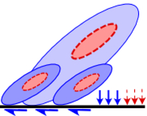
1. Introduction and motivation

Wall-bounded flows are ubiquitous in various applications, such as over aircraft wings and around submarines, where they affect vessel performance through the imposition of wall-shear-stress (${\tau }_{w}$) and wall-pressure ($\,p_{w}$) fluctuations on the bounding surface. The former, ${\tau }_w$, are associated with the skin-friction drag which limits vehicle speed, while the latter, $p_w$, are responsible for flow-induced vibrations that affect structural stability and generate noise. Nevertheless, accurately modelling the fluctuations in ${\tau }_w$ and $p_w$ remains a challenge due to the limited understanding of the dependence of their generation mechanisms on the Reynolds number.

Figure 1 shows a compilation of premultiplied frequency spectra of ${\tau }_{w}$ and $p_{w}$ for a wide range of Reynolds numbers. Here, the viscous-scaled time is defined as $T^+ = {{{U}^2_{\tau }}}/(\,{f}{\nu })$, where $f$ is the frequency of turbulence scales, $\nu$ is the kinematic viscosity and ${U}_{\tau }$ is the mean friction velocity, with superscript ‘+’ indicating viscous scaling. All these spectra have been computed from previously published high-fidelity simulations ($500 \lesssim Re_{\tau } \lesssim 2000$) and experimental data sets ($ {O}(10^4) \lesssim Re_{\tau } \lesssim {O}(10^6)$) of a turbulent boundary layer (TBL), where $Re_{\tau } = {U}_{\tau }{\delta }/{\nu }$ is the friction Reynolds number and $\delta$ is the TBL thickness. Although the experimental spectra have certain limitations at $T^+ \lesssim 100$ owing to spatial and temporal resolution, they will not influence this discussion (see § 3).

Figure 1.

Premultiplied energy spectra of (a) ${\tau }_w$, (b) $p_w$ and (c) premultiplied spectrogram of the bulk turbulence production ($\,f{z^+}{P^+}$) as a function of $T^+ (= 1/{f^+})$. Data for $500 \lesssim Re_{\tau } \lesssim 2000$ are from Eitel-Amor, Örlü & Schlatter (Reference Eitel-Amor, Örlü and Schlatter2014), for $Re_{\tau } \sim {O}(10^4)$ are from Marusic et al. (Reference Marusic, Chandran, Rouhi, Fu, Wine, Holloway, Chung and Smits2021) and for $Re_{\tau } \sim {O}(10^6)$ are from the Surface Layer Turbulence and Environmental Science Test (SLTEST) facility data sets acquired by (a) Marusic & Heuer (Reference Marusic and Heuer2007) and (b) Klewicki, Priyadarshana & Metzger (Reference Klewicki, Priyadarshana and Metzger2008). Grey and yellow coloured backgrounds in (a–c) indicate the nominal intermediate ($ {O}(10^2) \lesssim T^+ \lesssim {O}(10^3)$) and large-scale ranges ($T^+ \gtrsim {O}(10^3)$), respectively.

A noteworthy observation from figure 1(a,b) is the increasing energy contribution to the ${\tau }_w- (T^+ \gtrsim {O}(10^3))$ and $p_w$-spectra ($T^+ > {O}(10^2)$) with increasing $Re_{\tau }$, which has been noted previously in all canonical wall flows (Tsuji et al. Reference Tsuji, Fransson, Alfredsson and Johansson2007; Örlü & Schlatter Reference Örlü and Schlatter2011; Mathis et al. Reference Mathis, Marusic, Chernyshenko and Hutchins2013; Panton, Lee & Moser Reference Panton, Lee and Moser2017; Yu, Ceci & Pirozzoli Reference Yu, Ceci and Pirozzoli2022; Baars, Dacome & Lee Reference Baars, Dacome and Lee2024). While these viscous-scaled spectra exhibit $Re_{\tau }$-invariance in the small-scale range ($T^+ \lesssim 100$), they exhibit distinct $Re_{\tau }$-variations in the intermediate ($O(10^2) \lesssim T^+ \lesssim O(10^3)$) and large-scale ranges ($T^+ \gtrsim O(10^3)$), with these nominal bounds considered based on the largest possible $Re_{\tau }$-range (figure 1a,b). Although past studies have broadly linked these $Re_{\tau }$ trends to the energization of large inertial motions, the present study addresses two fundamental questions that have remained unanswered: (i) Which motions are responsible for transporting the large-scale energy (i.e. energy of large-scale motions), residing in the outer region, towards the wall to influence the wall-shear stress (Lee & Moser Reference Lee and Moser2019; Lee & Hwang Reference Lee and Hwang2024)? (ii) Which motions contribute to the rapid $Re_{\tau }$-growth of $p_w$ in the intermediate scales ($O(10^2) \lesssim T^+ \lesssim O(10^3)$), and why is this growth relatively weaker in the case of ${\tau }_w$?

The origin of the large-scale inertia-dominated energy in the outer region has now been well established in the literature (Lee & Moser Reference Lee and Moser2019), based on the turbulent kinetic energy (TKE) production term, $P^+ = -2{{\overline {uw}}^+}({{\partial }{{{U}}^+}}/{{\partial }{z^+}})$. Here, $u$, $v$ and $w$ represent instantaneous velocity fluctuations along the streamwise ($x$), spanwise ($\kern0.06em y$) and wall-normal ($z$) directions, respectively, while capital letters and overbar indicate time averaging. Figure 1(c) shows the premultiplied spectra of the bulk turbulence production ($\,f{z^+}{P^+}(z^+; T^+)$) from the same simulation data sets as in figure 1(a,b). Note here that the premultiplication with $z^+$ artificially amplifies the spectral content in the outer region compared with the inner region, but the majority of the energy production essentially occurs near the wall when $Re_{\tau } \lesssim {O}(10^3)$. Figure 1(c) confirms the weak energy production in the near-wall large scales ($T^+ > 1000$) compared with the small scales, thereby suggesting association of the large-scale ${\tau _w}-$signatures with wall-ward energy transport from the outer region (Lee & Hwang Reference Lee and Hwang2024). While several past studies have quantified and predicted the superposition of large-scale signatures on ${\tau }_w$ (Metzger & Klewicki Reference Metzger and Klewicki2001; Örlü & Schlatter Reference Örlü and Schlatter2011; Mathis et al. Reference Mathis, Marusic, Chernyshenko and Hutchins2013), fundamental understanding of their energy-transfer mechanisms is still lacking, starting from the motions governing the transport of large-scale energy from outer region towards the wall.

With regards to the differences between ${\tau }_w$ and $p_w$ over $ {O}(10^2) \lesssim T^+ \lesssim {O}(10^3)$, although considerable TKE is produced in this scale range in the inner region, the contour levels of the TKE production spectra in figure 1(c) exhibit a convincing collapse/invariance across different $Re_{\tau }$. This suggests a negligible $Re_{\tau }$-increment in the near-wall TKE production in the intermediate-scale range ($ {O}(10^2) \lesssim T^+ \lesssim {O}(10^3)$), consistent with results presented by Lee & Moser (Reference Lee and Moser2019). It means that the $Re_{\tau }$ increase of $f{{\phi }^{+}_{{{p}_w}{{p}_w}}}$ in the intermediate-scale range is also associated with the energization of turbulence motions farther away from the wall, which, however, seem to influence $f{{\phi }^{+}_{{{\tau }_w}{{\tau }_w}}}$ relatively weakly. The present study attempts to advance our fundamental understanding of the turbulence motions governing these trends, and their roles in the underlying energy-transfer mechanisms. This information would be valuable for designing high$-Re_{\tau }$ drag and noise reduction strategies in the future.

2. Active and inactive components and their roles in the energy-transfer mechanisms

This study explores the ability of the attached-eddy (i.e. wall-scaled eddy; Townsend Reference Townsend1976) framework to provide a phenomenological explanation for the questions raised above. This is motivated by the fact that the same framework has been previously successful in predicting the ${\tau }_w$- and $p_w$-spectra, associated with the inertial scales, across a broad $Re_{\tau }$-range (Ahn, Graham & Rizzi Reference Ahn, Graham and Rizzi2010; Marusic et al. Reference Marusic, Chandran, Rouhi, Fu, Wine, Holloway, Chung and Smits2021). Per Townsend's hypothesis, the outer region ($z \gtrsim z_{min}$) of a high$-Re_{\tau }$ wall-bounded flow can be statistically represented by a hierarchy ($ {O}(z_{min}) \lesssim \mathcal {H} \lesssim {O}(\delta )$) of geometrically self-similar, inviscid, wall-scaled eddies dominated by inertia (figure 2), where $\mathcal {H}$ is the eddy height and $z_{min}$ is the nominal lower bound of the log region. These wall-scaled eddies have been classically referred to as attached eddies in the literature, in reference to their scaling with $z$ and ${U}_{\tau }$, and not necessarily implying their physical extension to the wall. Townsend (Reference Townsend1976) proposed that these eddies have a population density varying inversely to their height $\mathcal {H}$, leading their cumulative velocity contributions at $z \gtrsim z_{min}$ to follow (at asymptotically high $Re_\tau$)

(2.1)\begin{equation} \left. \begin{aligned} {{\overline{u^2}}^+} & = {B_1} - {A_1} \ln({z}/{\delta}), \\ {{\overline{v^2}}^+} & = {B_2} - {A_2} \ln({z}/{\delta}), \\ {{\overline{w^2}}^+} & = {B_3}\quad \text{and} \\ {{\overline{uw}}^+} & = {B_4}, \end{aligned} \right\} \end{equation}

where $B_{1-4}$ and $A_{1-2}$ are constants. The increased availability of high-$Re_{\tau }$ data over the past two decades has provided considerable empirical support to these expressions (Jimenez & Hoyas Reference Jimenez and Hoyas2008; Hultmark et al. Reference Hultmark, Vallikivi, Bailey and Smits2012; Lee & Moser Reference Lee and Moser2015; Orlandi, Bernardini & Pirozzoli Reference Orlandi, Bernardini and Pirozzoli2015) in the nominal log region of the TBL (the exact definition of which may vary in the literature). The disagreement beyond the log region is owing to the statistical significance of the non-wall-scaled eddy-type motions coexisting in boundary layers, particularly in the boundary layer wake region (Marusic & Perry Reference Marusic and Perry1995).

Figure 2.

Conceptual sketches of wall-scaled eddies in a TBL at relatively (a) low ($Re_{{\tau }_1}$) and (b) high ($Re_{{\tau }_2}$) Reynolds numbers. (c–e) Depict the roles of the active and inactive parts of wall-scaled eddies in the energy-transfer mechanisms per the hypotheses of Bradshaw (Reference Bradshaw1967) and de Giovanetti, Hwang & Choi (Reference de Giovanetti, Hwang and Choi2016). Blue and red sections, respectively, correspond to the inactive and active portions of the wall-scaled eddies (grey scaled), which are defined based on the point of observation, $z$: (c) $z_1$ or (d,e) $z_2$. In (d,e), white eddies with dashed contours are centred lower than $z$, and hence are not involved in either local TKE production at $z$ (red region), or non-local energy transport from $z$ to the wall (cyan arrows). Greater thickness of the arrows in (e) indicates larger transport magnitude at higher $Re_{\tau }$. Panels show (a) $Re_{{\tau }_1}$; (b) $Re_{{\tau }_2}>Re_{{\tau }_1}$; (c) $Re_{{\tau }_1}$, point of observation: $z_1$; (d) $Re_{{\tau }_1}$, point of observation: $z_2$; (e) $Re_{{\tau }_2}$, point of observation: $z_2$.

While the expressions for ${\overline {u^2}}^+$ and ${\overline {v^2}}^+$ in (2.1) suggest their dependence on $Re_{\tau }$, ${\overline {w^2}}^+$ and ${\overline {uw}}^+$ are postulated to be $Re_{\tau }$-independent in the large $Re_{\tau }$ limit. Townsend (Reference Townsend1976) explained this contradiction by proposing that the flow at any point of observation ($z \gtrsim z_{min}$) comprises two components of wall-scaled eddies (figure 2) – an ‘active’ component of the wall-scaled eddy that is responsible for local turbulent transfer and accounts for the instantaneous Reynolds shear stresses ($uw$) at $z$, and an ‘inactive’ component that does not contribute to $uw$ at $z$. Here, the inactive component predominantly comes from wall-scaled eddies much taller than $z$, which contribute to $uw$ (i.e. behave as active motions) at wall-normal locations larger than $z$. Hence, while the active component is solely responsible for the local TKE production, Townsend (Reference Townsend1976) described inactive motions as non-local ‘swirling motions’ whose ‘effect on that part of the layer between the point of observation and the wall is one of slow random variation of ‘mean velocity’ which cause corresponding variation of wall stress’. These statements were supported by Bradshaw (Reference Bradshaw1967) and de Giovanetti et al. (Reference de Giovanetti, Hwang and Choi2016), who hypothesized that the inactive parts of the wall-scaled eddies are responsible for transporting large-scale energy produced in the outer layer (by active parts), to the wall. As per Bradshaw (Reference Bradshaw1967), this process is necessary to maintain the near-wall energy balance and is sketched in figure 2(c–e).

Although the non-local wall-normal transport of large-scale energy has been previously observed through correlation/spectral analysis of the TKE budget equations (Cho, Hwang & Choi Reference Cho, Hwang and Choi2018; Lee & Moser Reference Lee and Moser2019; Yin, Hwang & Vassilicos Reference Yin, Hwang and Vassilicos2024), its connection with the inactive part of the wall-scaled eddies has never been definitively established, primarily due to the lack of a reliable flow-decomposition methodology. Along the same lines, while the association of $p_w$-signatures with intense $uw$ events is well known (Gibeau & Ghaemi Reference Gibeau and Ghaemi2021; Baars et al. Reference Baars, Dacome and Lee2024), their distinct correlations with $uw$-contributing (active) and non-contributing (inactive) components has never been explicitly established. Recently, Deshpande, Monty & Marusic (Reference Deshpande, Monty and Marusic2021) proposed a spectral linear stochastic estimation (SLSE)-based methodology that enables data-driven decomposition of the log-region flow into its corresponding active and inactive components. This provides an opportunity to establish the association of active/inactive components with ${\tau }_w$ and $p_w$, and thereby explain their $Re_{\tau }$-variation based on the $Re_{\tau }$ growth of the wall-scaled eddy hierarchy (figure 2).

2.1. Revisiting the concept of active and inactive motions

Before proceeding with the new analysis, we briefly review the concept of active and inactive motions by means of a simplified mathematical description, which is inspired by Townsend's original ideas and adapted from our previous work (Deshpande, Monty & Marusic Reference Deshpande, Monty and Marusic2020; Deshpande et al. Reference Deshpande, Monty and Marusic2021). We consider the simplest model of a wall-bounded flow comprising wall-scaled eddies as the only eddying motions, which are represented by hairpin-type vortical structures. It is important to note here, however, that the concept of active and inactive motions does not depend on the shape of the vortical structures, but is rather associated with the spatial distribution of velocity signatures generated by these vortical structures, as depicted in figure 3(a) (estimated by simple Biot–Savart calculations). The inviscid nature of the wall-scaled eddy model permits slip at the wall (i.e. finite $u$ and $v$), while $w = 0$ is enforced at $z = 0$ to remain consistent with wall impermeability. These differences in the boundary conditions result in spatially localized $w$-signatures (and consequently $uw$-signatures) at $z$ from any wall-scaled eddy of $\mathcal {H} \sim {O}(z)$, while the $u$- and $v$-signatures extend across 0 $\lesssim z < \mathcal {H}$ (i.e. non-local; refer to figure 3a). It is these characteristics that distinguish the active and inactive contributions in the velocity flow field, despite both of them originating from the same wall-scaled vortical structures.

Figure 3.

(a) Spatial signatures of the three velocity components ($u,v,w$) from a hairpin-type vortex structure of height $\mathcal {H}$, representative of a wall-scaled eddy (Marusic & Perry Reference Marusic and Perry1995). Regions in magenta and indigo, respectively, denote high- and low-momentum regions for the corresponding velocity fluctuations. (b) Eddy-intensity functions ($I_{ij}$) for wall-scaled eddies of three different heights ${\mathcal {H}}_i$, with ${\mathcal {H}}_1 < {\mathcal {H}}_2 < {\mathcal {H}}_3$. Here, $u_i,v_i,w_i$ respectively denote velocity signatures generated from these wall-scaled eddies that are sensed by a probe, depending on their $z$-location. Red and blue background shadings of $u_i,v_i,w_i$, respectively, indicate active and inactive contributions at that location. The figure has been adapted from Deshpande et al. (Reference Deshpande, Monty and Marusic2020).

Differences in the active/inactive contributions to the Reynolds stresses can be understood by invoking Townsend's (Reference Townsend1976) eddy-intensity function $I_{ij}$ (where $i,j = u$, $v$ or $w$), depicted schematically in figure 3(b) for the four non-zero combinations of $i,j$ (refer to (2.1)). Here, $I_{ij}$ is representative of the contribution from each eddy to the normal and Reynolds shear stresses as a function of $z$, and this is sketched for wall-scaled eddies of three different heights ($\mathcal {H}_{1}$–$\mathcal {H}_{3}$) in figure 3(b), as an example. Effects of increasing $Re_{\tau }$ can be accounted for by including taller eddies of height ${\mathcal {H}}_4 > {\mathcal {H}}_3$ and so on. The wall-normal distributions of $I_{ij}$ are inspired by the individual velocity distributions in figure 3(a), and they are used to explain the cumulative contributions to the Reynolds stresses (from the three eddies) at three different probe locations in figure 3(b). For instance, when the probe is positioned at $z \sim \mathcal {H}_{1}$, all three eddies will contribute to $\overline {u^2}(z)$ and $\overline {v^2}(z)$, while the contribution to $\overline {w^2}(z)$ and $\overline {uw}(z)$ would come solely from the eddy of height $\mathcal {H}_{1}$. However, upon increasing the probe location to $z \sim \mathcal {H}_{2}$, contributions to the wall-parallel stresses are only made by the tallest two eddies, while those to $\overline {w^2}(z)$ and $\overline {uw}(z)$ only come from the eddy of height $\mathcal {H}_{2}$, and so on. Connecting these observations with Townsend's definitions in § 2, the active contributions at any $z$ can be solely associated with eddies of height, $\mathcal {H} \sim {O}(z)$, which will contribute to $u$, $v$, $w$ and hence $uw$, at $z$ (indicated by red background shading in figure 3b). On the other hand, the inactive contributions are associated with relatively tall wall-scaled eddies: $ {O}(z) \ll \mathcal {H} \lesssim {O}(\delta )$. These contribute to $u(z)$ and $v(z)$, but not $w(z)$ and $uw(z)$ (indicated by blue background shading).

Considering that increasing $Re_{\tau }$ introduces new eddies that are much taller than $z$, only the inactive contributions to $u(z)$ and $v(z)$ will increase for all $z \ll \mathcal {H}$, while the active contributions will exhibit $Re_{\tau }$-invariance when scaled in wall units (i.e. $z$ and $U_{\tau }$). This explains the contrasting trends exhibited by the Reynolds stresses in (2.1), where ${\overline {u^2}}^+(z)$ and ${\overline {v^2}}^+(z)$ are $Re_{\tau }$-dependent while ${\overline {w^2}}^+(z)$ and ${\overline {uw}}^+(z)$ exhibit $Re_{\tau }$-invariance in the log region. In summary, both active and inactive motions contribute to the wall-parallel velocity fluctuations, but only the former contribute to the Reynolds shear stresses and $w$-fluctuations. This is expressed mathematically by the following (Panton Reference Panton2007; Deshpande & Marusic Reference Deshpande and Marusic2021):

(2.2)\begin{equation} \left. \begin{aligned} {u}(z) & = {u_{a}}(z) + {u_{ia}}(z),\\ {v}(z) & = {v_{a}}(z) + {v_{ia}}(z)\quad \text{and} \\ {w}(z) & = {w_{a}}(z), \end{aligned} \right\} \end{equation}

where subscripts ‘${a}$’ and ‘${ia}$’, respectively, denote active and inactive components. The variances can be decomposed according to the following (Panton Reference Panton2007; Deshpande & Marusic Reference Deshpande and Marusic2021):

(2.3)\begin{equation} \left. \begin{aligned} {{\overline{u^2}}^+} & = {{\overline{u^2_{ia}}}^+} + {{\overline{u^2_{a}}}^+} + 2\overline{{u_{ia}}{u_{a}}},\\ {{\overline{v^2}}^+} & = {{\overline{v^2_{ia}}}^+} + {{\overline{v^2_{a}}}^+} + 2\overline{{v_{ia}}{v_{a}}},\\ {{\overline{w^2}}^+} & = {{\overline{w^2_{a}}}^+} \quad \text{and} \\ {{\overline{uw}}^+} & = {{\overline{{u_{a}}{w}}}^+} + {{\overline{{u_{ia}}{w}}}^+}. \end{aligned} \right\} \end{equation}

While $\overline {{u_{ia}}{u_{a}}}$, $\overline {{v_{ia}}{v_{a}}}$ and $\overline {{u_{ia}}{w}} = 0$ for a traditionally conceptualized wall-scaled eddy field (i.e. considering only linear superposition of velocity fluctuations originating from various hierarchies of wall-scaled eddies), that is not true for an actual/real wall-bounded flow (Deshpande et al. Reference Deshpande, Monty and Marusic2021; Deshpande & Marusic Reference Deshpande and Marusic2021). A real TBL also comprises very-large-scale inertial motions/superstructures that are inherently inactive per the definition of Townsend (Deshpande et al. Reference Deshpande, Monty and Marusic2021) and interact nonlinearly with/modulate the eddies local to $z$ (Metzger & Klewicki Reference Metzger and Klewicki2001; Mathis et al. Reference Mathis, Marusic, Chernyshenko and Hutchins2013; Baars, Hutchins & Marusic Reference Baars, Hutchins and Marusic2016). The causality between superstructures and nonlinear interactions, however, is a topic of ongoing debate (Andreolli et al. Reference Andreolli, Gatti, Vinuesa, Örlü and Schlatter2023). This, combined with the fact that these nonlinear interactions are smaller in magnitude than individual $\overline {u^2_{ia}}$ and $\overline {u^2_{a}}$ components (Deshpande & Marusic Reference Deshpande and Marusic2021), makes the investigation of nonlinear interactions beyond the scope of this study. The present study aims to deploy the decomposition methodology facilitating (2.2) on instantaneous flow fields of published data sets, to analyse for the first time the active and inactive contributions to ${\tau }_w$ and $p_w$. This work builds on the past successes of the decomposition methodology (Deshpande et al. Reference Deshpande, Monty and Marusic2021) that has yielded empirical support for the scaling characteristics of the active and inactive components, hypothesized by Townsend (Reference Townsend1976). This includes the $z$-scaling behaviour of ${{\overline {u^2_{a}}}^+}$, and the inverse-logarithmic variation of ${{\overline {u^2_{ia}}}^+}$ associated with the $k^{-1}$-scaling (where k represents the streamwise/spanwise wavenumber), to list a few.

3. Data sets and methodology

The present study considers two previously published multi-point data sets across a large $Re_{\tau }$ range: $ {O}(10^3) \lesssim Re_{\tau } \lesssim {O}(10^6)$, for the SLSE analysis. The low$-Re_{\tau }$ data set is from the high-resolution large-eddy simulation (LES) of a zero-pressure-gradient TBL by Eitel-Amor et al. (Reference Eitel-Amor, Örlü and Schlatter2014), which was computed over a numerical domain large enough for the TBL to evolve up to $Re_{\tau } \approx 2000$. In comparison with a fully resolved direct numerical simulation (DNS), the resolution employed in the LES data is just a factor of 2 coarser in the wall-parallel directions, and approximately 1.5 times coarser along the wall-normal one. Hence, instead of using a conventional subgrid-scale model in the simulation, a small forcing was implemented on the very small scales, essentially to add some extra dissipation. As a consequence, only two minor statistical differences emerge compared with a fully resolved DNS: a slight attenuation of the near-wall peak of ${\overline {u^2}}^+$, and a resolved TKE dissipation 87.2 % of that in a conventional DNS. However, adding the dissipation associated with the forcing recovers 99.8 % of the TKE dissipation. Since the present study predominantly focuses on the correlation between synchronously sampled time series of the desired wall properties (${\tau }^+_w$, ${p}^+_w$) and the overlying flow field ($u^+$, $w^+$), the use of a high-resolution LES instead of DNS does not influence the present conclusions. These correlations are investigated at designated streamwise locations of the numerical domain, corresponding to $Re_{\tau } \approx 500, 1000, 1500$ and 2000. For this, the time series of the LES were sampled across the entire domain cross-section ($\kern0.06em y-z$), with a resolution of ${\Delta }t^+ \lesssim 0.5$ and for a total eddy-turnover time (${t_{samp}}{U_{\infty }}/{\delta }) \approx 243$, where $U_\infty$ is the free-stream speed. Combined with the option to ensemble average across the span, these time series are long enough to obtain a sufficiently converged frequency spectrum for capturing the inertial phenomena (demonstrated in Eitel-Amor et al. Reference Eitel-Amor, Örlü and Schlatter2014).

The high-$Re_{\tau } (\sim {O}(10^6))$ data set is from the neutrally buoyant surface layer at the SLTEST facility in Utah (Marusic & Heuer Reference Marusic and Heuer2007). The data comprise synchronously acquired time series of ($u^+$, $w^+$) from five sonic anemometers positioned on a vertical tower, within the log region ($0.0025 < z/{\delta } < 0.0293$), and wall-shear-stress signals (${\tau }^+_w$) measured using a custom-designed sensor placed vertically below the sonics. These data were acquired at a time resolution of ${\Delta }t^+ \lesssim 78.4$ and for a total of 175 eddy-turnover times, across a viscous-scaled measuring volume of 1400 (of sonics).

While the sampling intervals for both LES and SLTEST data sets are not sufficient for fully converging/resolving the very-large-scale phenomena (quantitatively), they have been analysed previously by Deshpande, Vinuesa & Marusic (Reference Deshpande, Vinuesa and Marusic2024) and found to be sufficient to attain an accurate qualitative understanding. This was demonstrated by repeating the same statistical analysis (as presented ahead in § 3.1) on the simultaneous $u^+,w^+$ and ${\tau }^+_w$ measurements conducted in the large Melbourne wind tunnel (Deshpande & Marusic Reference Deshpande and Marusic2021), time series for which were sampled for a much longer time interval and at greater frequency. The results and trends derived from the wind-tunnel data were qualitatively consistent with those obtained from the LES and SLTEST data sets, which will serve as the basis for the present study. Both these data sets provide rare access to velocity-fluctuation time series across the log region synchronously with ${\tau }_w$, for TBLs spanning a broad $Re_{\tau }$ range ($10^3$–$10^6$). This offers a unique opportunity to directly test the hypotheses of Bradshaw (Reference Bradshaw1967) and de Giovanetti et al. (Reference de Giovanetti, Hwang and Choi2016), regarding TKE production and transport mechanisms from the log region to the wall, and to understand how they affect ${\tau }_w$ and $p_w$. Our present conclusions will only depend on the qualitative energy variation across $z$, and not focus on its quantification/scaling (requiring convergence). We note that, although the SLTEST flows are transitionally rough TBLs, the roughness effects are insignificant beyond the roughness sublayer (Klewicki et al. Reference Klewicki, Priyadarshana and Metzger2008; Marusic & Heuer Reference Marusic and Heuer2007). Hence, the roughness will not influence the inertial eddies, which are our primary focus.

3.1. Data-driven flow-decomposition methodology

The multi-point nature of both the LES and SLTEST data sets permits theoretical estimation of $u_{a}$ and $u_{ia}$ by following the SLSE-based methodology proposed previously in Deshpande et al. (Reference Deshpande, Monty and Marusic2021) and Deshpande & Marusic (Reference Deshpande and Marusic2021). Throughout this paper, we limit our SLSE analysis to the log region where the concept of active and inactive motions, as well as expressions in (2.1), have received considerable empirical support (Deshpande et al. Reference Deshpande, Monty and Marusic2021). Per the SLSE methodology (Baars et al. Reference Baars, Hutchins and Marusic2016), the instantaneous component $u_{ia}(z)$ in the log region can be obtained by

(3.1)\begin{equation} {\widetilde{u_{ia}}}(z^{+};{T^{+}}) = {{H_{L}}(z^{+};{T^{+}})}{\widetilde{u_{\tau}}}({T^{+}}). \end{equation}

Here, ${\widetilde {u_{\tau }}}(T^+) = \sqrt {{\widetilde {{\tau }_{w}}}/{\rho }} = \mathcal {F}(u_{\tau }(t^+))$ is essentially the Fourier transform of the friction velocity fluctuations, $u_{\tau }(t^+)$, in time $t$, where $\rho$ is density. The parameter ${\widetilde {u_{\tau }}}$ acts as the scale-specific unconditional input required to obtain the scale-specific conditional output, ${\widetilde {u_{ia}}}(z^{+};{T^{+}})$. The linear relationship between $\widetilde {u_{ia}}$ and $\widetilde {u_{\tau }}$ is inspired by the original definitions of active and inactive motions derived from the wall-scaled eddy model (refer § 2), which assumes a linear superposition of the velocity signatures generated by individual eddies. Further, $H_{L}$ is the complex-valued linear transfer kernel reconstructed by cross-correlating the synchronously acquired $\tilde {u}(z^+)$ and $\widetilde {u_{\tau }}$ according to the following:

(3.2)\begin{equation} {H_{L}}(z^{+};{T^{+}}) = \frac{ \{ \tilde{u}(z^{+};{T^{+}}){{\widetilde{u_{\tau}}}^{{\ast}}}({T^{+}}) \} }{ \{ {{\widetilde{u_{\tau}}}({T^{+}})}{{\widetilde{u_{\tau}}}^{{\ast}}}({T^{+}}) \} }, \end{equation}

where the curly brackets ($\{{\cdot } \}$) and asterisk ($\ast$) denote ensemble averaging and complex conjugate, respectively. Here, the definition of $H_{L}$ is underpinned by the discussion presented in § 2 and figure 3 that the inactive components coexisting at $z^+$ extend down to the wall (i.e. influence $u_{\tau }$), while the active components are localized to $z$. Hence, (3.1) and (3.2) essentially classify $\widetilde {u_{ia}}$ as a subset of the total momentum $\tilde {u}$ that is coherent with $\widetilde {u_{\tau }}$. Figure 4(a,b) depicts $|H_{L}|({z^+}, T^+)$ computed from the LES and SLTEST data sets at $z^+$ within the log region, alongside the premultiplied spectra of $u_{\tau }$ ($\,{f}{{\phi }^+_{{u_{\tau }}{u_{\tau }}}}$), where $|{{\cdot }}|$ represents the modulus. Before plotting, $|H_{L}|$ has been smoothed based on a 25 % bandwidth moving filter (Baars et al. Reference Baars, Hutchins and Marusic2016). This is done to remove the noise emerging from the mathematical operations in (3.2), which are conducted on a per-scale basis. It is evident that $|H_L|$ is non-zero across a broadband range of $T^+$ when $z$ is close to the lower bound of the log region. However, $|H_L|$ gets restricted to relatively large scales with an increase in $z^+$, essentially acting as a $z$-dependent low-pass filter conforming to larger scales with increasing $z$, in a manner consistent with Townsend's wall-scaled eddy hypothesis (refer § 2). These trends also align with the $|H_L|$ computed previously using long time-series signals from the Melbourne wind-tunnel data (Deshpande & Marusic Reference Deshpande and Marusic2021; Deshpande et al. Reference Deshpande, Vinuesa and Marusic2024), confirming they are physical and not artefacts of insufficient convergence.

Figure 4.

Absolute values of the linear transfer kernel ($|H_L|(z^+;T^+$); (3.2)) computed for the (a) LES and (b) SLTEST data with grey shading representing changing $z^+$. Here, $|H_L|$ is plotted for $z^+$ limited to the log region and its ordinate is considered on the primary vertical axis (left; in black) while the solid golden line represents the premultiplied spectra of the friction velocity ($\,f{{\phi }^+_{{u_{\tau }}{u_{\tau }}}}$) and its ordinate is considered on the secondary vertical axis (right; in golden yellow). (c,d) Premultiplied spectra of the active ($u_{a}$) and inactive $u$-components ($u_{ia}$) estimated for various $z$-locations in the log region for both the LES and SLTEST data. Note that the horizontal axis is chosen to test for $z$-scaling of the spectra by invoking Taylor's hypothesis. Panels show data for (a) $Re_{\tau } \approx 2000$, (b) $Re_{\tau } \approx {O}(10^6)$, (c,d) both $Re_{\tau}\approx 2000$ and $Re_{\tau}\approx O(10^6)$.

Significantly, for both the LES and SLTEST data, $|H_{L}|$ extends to sufficiently large $T^+$ values where the corresponding $f{{\phi }^+_{{u_{\tau }}{u_{\tau }}}}$ is negligible beyond the considered range. This ensures proper estimation of the very-large-scale ${\widetilde {u_{ia}}}$ signal. Similarly, the time resolution and frequency response of the wall-shear-stress sensor at high $Re_{\tau }$, despite limiting the measurement of the wall-shear-stress spectrum to $T^+ \gtrsim$ 1000 (figures 1a and 4b), is sufficient to resolve ${\widetilde {u_{ia}}}$ considering $|H_{L}| \sim 0$ at $T^+ \lesssim 1000$. The efficacy of extracting the inactive contributions is demonstrated by examining the scaling characteristics of the premultiplied $u_{ia}$-spectra ($\,f{{\phi }^+_{{u_{ia}}{u_{ia}}}}$; also see Deshpande et al. Reference Deshpande, Monty and Marusic2021). Figure 4(d) depicts $f{{\phi }^+_{{u_{ia}}{u_{ia}}}}$ estimated for various $z/{\delta }$ in the log region for the two data sets, and it is plotted against $z$-scaled streamwise wavelengths (${T^+}{U^+}(z^+)/z^+$) computed based on Taylor's hypothesis (well accepted for inertial scales below 6$\delta$; Dennis & Nickels Reference Dennis and Nickels2008). Considering that inactive contributions at any $z$ are associated with wall-scaled eddies across $ {O}(z) \lesssim \mathcal {H} \lesssim {O}(\delta )$, $f{{\phi }^+_{{u_{ia}}{u_{ia}}}}$ is expected to exhibit $z$-scaling only in the relatively small-scale range, consistent with the trends in figure 4(d). Further, it is evident that the relatively large-scale contributions to $f{{\phi }^+_{{u_{ia}}{u_{ia}}}}$ decrease with $z/{\delta }$ across both data sets, which is also consistent with the inverse-logarithmic variation of $\overline {u^2_{ia}}$ expected based on the wall-scaled eddy hypothesis (refer to § 2 and Deshpande et al. Reference Deshpande, Monty and Marusic2021).

Once ${\widetilde {u_{ia}}}$ is obtained via (3.1), its time-domain equivalent can be calculated simply by taking the inverse Fourier transform (Deshpande & Marusic Reference Deshpande and Marusic2021) ${{{u}_{ia}}(z^{+}; {t^{+}})} = {\mathcal {F}^{-1}}({{\widetilde {{u}_{ia}}}(z^{+};{T^{+}})})$. Considering the discussion on the past hypotheses in § 2, the novel analysis here is not to establish the correlation of $u_{ia}$ with ${\tau }_w$ (which is imposed by definition in (3.1)), but to investigate the variation of simultaneously acquired $u_{ia}$-signals across various $z$-locations in the log region (see § 4.1). Estimation of $u_{ia}$ also permits calculation of the $u_{a}$-time series by simple subtraction, ${{{u}_{a}}(z^{+};{t^{+}})} = {{{u}}(z^{+};{t^{+}})}$ – ${{{u}_{ia}}(z^{+};{t^{+}})}$, thereby associating $u_{a}$ with the $u$-subset that is incoherent with the wall (i.e. $u_{\tau }$). Similar to the investigation of $f{{\phi }^+_{{u_{ia}}{u_{ia}}}}$, we can examine the premultiplied $u_{a}$-spectrum ($\,f{{\phi }^+_{{u_{a}}{u_{a}}}}$) for its expected scaling arguments. Per Townsend's (Reference Townsend1976) hypothesis, active contributions at $z$ are solely associated with wall-scaled eddies of $\mathcal {H} \sim {O}(z)$, suggesting $f{{\phi }^+_{{u_{a}}{u_{a}}}}$ should exhibit $z$-scaling irrespective of the flow $Re_{\tau }$. Figure 4(c) depicts reasonably good $z$-scaling of the premultiplied $u_{a}$-spectra across $ {O}(10^3) \lesssim Re_{\tau } \lesssim {O}(10^6)$, consistent with the previous findings in Deshpande et al. (Reference Deshpande, Monty and Marusic2021). This ability to estimate $u_{a}$ enables computation of the Reynolds shear stresses associated exclusively with the active motions (${u_{a}}w(z^+; t^+)$), which should correspond closely with the net Reynolds shear stresses ($uw(z^+; t^+)$) per Townsend's (Reference Townsend1961) hypothesis. These hypotheses are tested in this study using simultaneously acquired time-series signals, across the log region, for the first time (see § 4.1).

5. Concluding remarks

This study clarifies the $Re_{\tau }$-dependent, intermediate- and large-scale contributions to the ${\tau }_w$- and $p_w$-spectra by invoking the attached (wall-scaled) eddy framework (Townsend Reference Townsend1976), based on active and inactive motions. Unique multi-point data sets are analysed using an energy-decomposition methodology to reveal the contributions from TKE-producing (active) and non-producing (inactive) components, at any wall-normal position in the log region, to the ${\tau }_w$- and $p_w$-spectra. Inactive components of wall-scaled eddies are found to be responsible for the non-local wall-normal transport of the large-scale inertia-dominated energy, from its origin in the log region (i.e. produced by active components) to the wall. On the other hand, the majority of the TKE-producing (i.e. active) motions in the log region are localized and physically detached from the wall, not influencing ${\tau }_w$. These results provide strong empirical evidence for the hypotheses proposed by Bradshaw (Reference Bradshaw1967) and de Giovanetti et al. (Reference de Giovanetti, Hwang and Choi2016). They also explain the appearance and $Re_{\tau }$-growth of the large-scale signatures in the ${\tau }_w$-spectra, despite the insignificant large-scale TKE production occurring in the near-wall region. In terms of their contribution to wall pressure, the active and inactive components are respectively correlated with the intermediate- and large-scale portions of the $p_w$-spectrum. Both components exhibit growth with increasing $Re_{\tau }$, which is attributed to the broadening of the wall-scaled eddy hierarchy. This is plausibly responsible for the rapid $Re_{\tau }$-growth of the $p_w$-spectra relative to ${\tau }_w$ (figure 1a,b). These phenomenological explanations carry potential to influence future real-time control strategies, aimed at achieving energy-efficient drag and flow-noise reduction.

While this study demonstrates the new found capability to extract the instantaneous active and inactive components, also shedding light on their role in the large-scale energy-transfer mechanisms, it does not delve into the nonlinear/inter-scale interactions between these motions. These interactions, which have been previously discussed in the literature to a certain extent (Cho et al. Reference Cho, Hwang and Choi2018; Lee & Moser Reference Lee and Moser2019), can likely explain the transfer of TKE produced by active components to the inactive component of the wall-scaled eddies, before being transported downward to the wall (figure 2). At this stage, these interactions are not accounted for within Townsend's wall-scaled eddy framework, which is inherently limited to the linear superposition of velocity signatures induced by the eddy structures. It does, however, highlight the opportunity for future upgrades/modifications to the model by incorporating the inter-scale interactions between the wall-scaled eddy hierarchy.