

INTRODUCTION
Sea-ice algae are important contributors to primary production in the polar oceans (McMinn and others, Reference McMinn2012; Arrigo and others, Reference Arrigo, Brown and Mills2014; Kohlbach and others, Reference Kohlbach2016) and play an active role in large-scale biogeochemical cycles determining rates of carbon export (Boetius and others, Reference Boetius2013) and ocean/atmosphere exchange (Vancoppenolle and others, Reference Vancoppenolle2013). During winter and spring, sea-ice algae are vital for polar marine ecosystems as they provide an essential food source for pelagic herbivores (Flores and others, Reference Flores2012; Arrigo and others, Reference Arrigo, Brown and Mills2014). During the melt season, ice algae can seed the spring phytoplankton bloom following ice ablation (Brugel and others, Reference Brugel2009; Søreide and others, Reference Søreide, Leu, Berge, Graeve and Falk-Petersen2010; Mundy and others, Reference Mundy2014).
Chlorophyll a (chl-a) concentrations in sea ice are considered a useful proxy for algal biomass abundance (Gradinger, Reference Gradinger2009; Meiners and others, Reference Meiners2012). The highest algal standing stocks are usually found at the bottom of the ice cover near the ice/water interface (Arrigo and others, Reference Arrigo, Mock, Lizotte, Thomas and Dieckmann2010). Using chl-a as proxy, several studies have reported high spatial variability in ice-algal biomass, for example changes across multiple orders of magnitude on spatial scales ranging from millimetres (Hawes and others, Reference Hawes2012) to the mesoscale (metres to kilometres) (Steffens and others, Reference Steffens2006; Gradinger, Reference Gradinger2009).
Unlike phytoplankton and ocean colour, chl-a concentrations in sea ice cannot be monitored with aerial or satellite remote-sensing techniques. Current sea-ice chl-a sampling methods include ice core sampling (Miller and others, Reference Miller2015), diver operated fluorometers (Rysgaard and others, Reference Rysgaard, Kühl, Glud and Hansen2001) or simple imagery data (such as video or still photographs) (Gutt, Reference Gutt1995; Katlein and others, Reference Katlein, Fernández-Méndez, Wenzhöfer and Nicolaus2015). These established methodologies are labour intensive, invasive or have a coarse resolution and are not appropriate for capturing the high spatial and temporal variability of ice-algae biomass. This has consequences for our understanding of ice-algal dynamics, with associated implications for estimating their overall contribution to marine production and how they respond to environmental changes (Meiners and others, Reference Meiners2012). Due to the high logistical costs involved in monitoring in the harsh polar environments, there is a need to develop new and efficient methodologies that can efficiently track ice-algal biomass across multiple spatial scales.
Recent studies have explored methods for quantifying chl-a (as proxy for biomass) within sea ice by measuring the spectral composition of downward transmitted visible light that is measured beneath the ice/water interface (Mundy and others, Reference Mundy, Ehn, Barber and Michel2007; Campbell and others, Reference Campbell, Mundy, Barber and Gosselin2014; Melbourne-Thomas and others, Reference Melbourne-Thomas2015). Transmitted light measurements at the ice bottom can provide information on algal biomass due to the light absorption by algal pigments such as chl-a (Maykut and Grenfell, Reference Maykut and Grenfell1975; Perovich, Reference Perovich1996). Quantitative methods are usually performed by deploying upward looking spectral irradiance sensors below the ice (at 15–50 cm distance) using an L-arm. The measured spectrum of transmitted irradiance can then be statistically correlated to the amount of measured chl-a (determined from ice core samples) using empirical correlations methods and univariate models such as Normalized Difference Indices (NDI) or Empirical Orthogonal Functions (EOFs) (Mundy and others, Reference Mundy, Ehn, Barber and Michel2007; Melbourne-Thomas and others, Reference Melbourne-Thomas2015; Lange and others, Reference Lange, Katlein, Nicolaus, Peeken and Flores2016). These novel methods are providing new opportunities for monitoring ice-algal biomass at an increased sampling rate in a non-invasive manner. For example, irradiance sensors can be mounted on Remotely Operated Vehicles (ROVs) for further enhancing the spatial extent of these surveys (Lange and others, Reference Lange, Katlein, Nicolaus, Peeken and Flores2016). The use of transmitted irradiance spectra, however, only determines the integrated (over the entire ice thickness) ice-algal biomass.
We are taking advantage of such considerations and for the first time we experimentally assess the possibility of employing hyperspectral imaging (HI) cameras in transmission mode (measuring transmitted instead of reflected light) to map sea-ice algae biomass distribution at the ice/water interface. In contrast to the wide and disconnected footprint of radiance and irradiance sensors, HI cameras are able to map spectral signatures across a target area at high spatial resolutions (Johnsen and others, Reference Johnsen2013; Amigo and others, Reference Amigo, Babamoradi and Elcoroaristizabal2015). HI is usually employed in reflectance mode and these systems are gaining considerable momentum in the natural sciences and close-range remote-sensing domain as the technology becomes more accessible and portable (e.g. Lucieer and others, Reference Lucieer, Malenovský, Veness and Wallace2014; Malenovský and others, Reference Malenovský, Turnbull, Lucieer and Robinson2015; Holzinger and others, Reference Holzinger, Allen and Deheyn2016). Recent applications in related disciplines include mapping of benthic algae distributions and biomass (Chennu and others, Reference Chennu2013), coral physiology (Perkins and others, Reference Perkins2016) and algae pigment composition (Nogami and others, Reference Nogami, Ohnuki and Ohya2014). Sea ice is an optically complex medium and there are many challenges in measuring transmitted radiance through the ice that need to be overcome through gradual testing and evaluation both in laboratory and in-situ studies. Aside from understanding the target spectral signature, we also need to understand the complexity associated with both under-ice HI deployment and data processing.
In the present study, a HI camera was used to image an inverted sea-ice simulation tank specifically designed for growing and monitoring sea-ice microbial consortia at the ice/water interface. The tank is termed ‘inverted’ due to its ‘upside down’ representation of the sea-ice environment, i.e. the light source is beneath the ice and a water layer is above it (Fig. 1). This configuration provides an ideal environment for testing different hyperspectral imaging scenarios in a controlled environment.
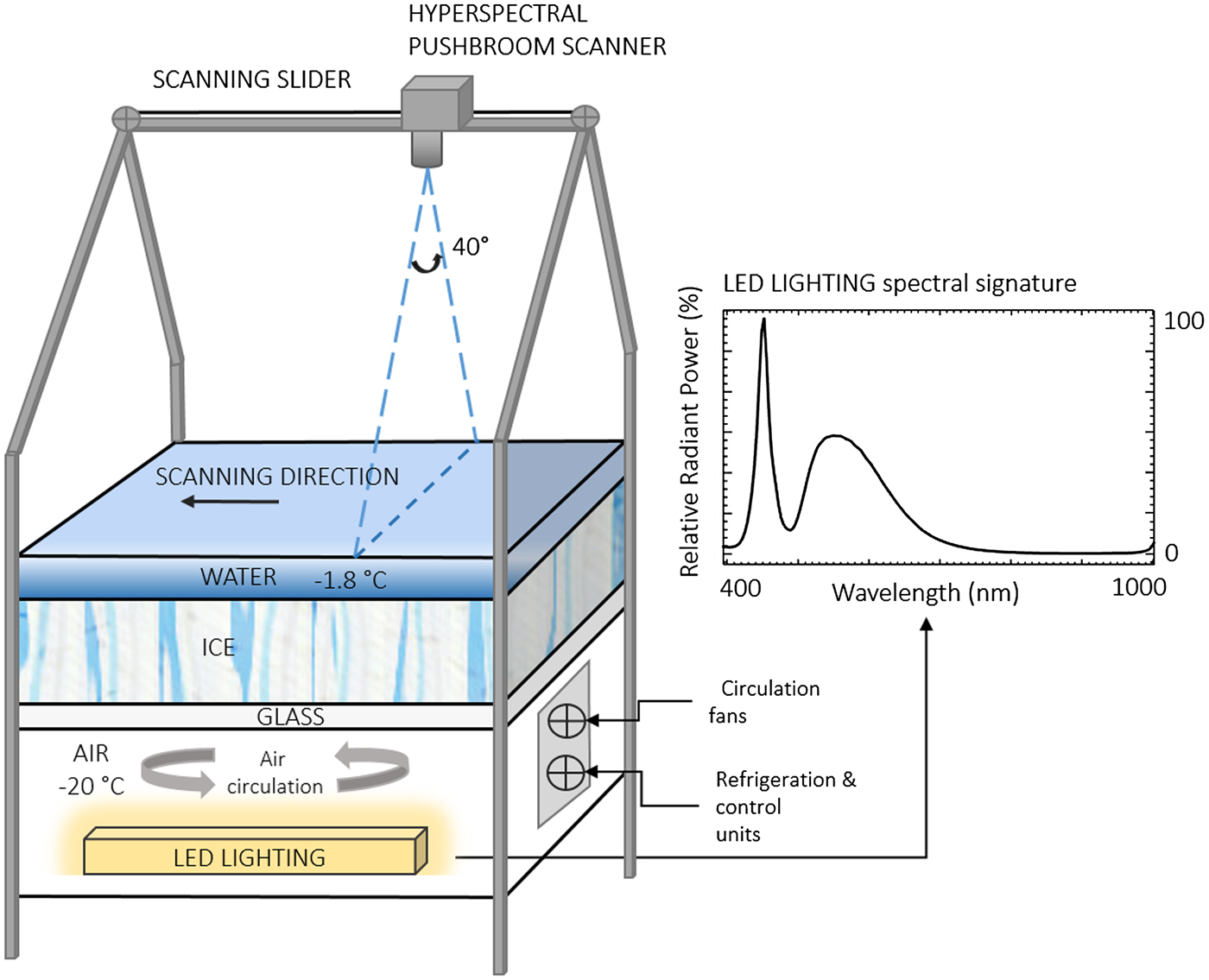
Illustration of the inverted sea-ice simulation tank and spectral signature of the LED artificial light source. The hyperspectral pushbroom scanner was mounted onto a motorized sliding rail at 1.2 m distance above the ice/water interface. The layered surfaces (glass, ice, water) cover an area of 0.85 m × 0.85 m. The distance from the camera fore-optics to the ice layer is 1 m. The illustration is not to scale.
This first test is a proof of concept, aimed to developing a near remote-sensing method that can identify ice-algae patchiness at multiple spatial scales in a non-invasive manner. For this purpose, we inoculated the tank with ice-algal communities to establish six spatially variable algal patches at the tank's ice/water interface. This study starts by outlining our novel experimental set-up and the data acquisition methodologies. We then employ exploratory image analysis to assess the feasibility of HI to resolve ice-algal spatial variability. The study concludes by comparing our sea-ice tank to an in-situ scenario and discussing future possibilities and limitations of the method.
DATA AND METHODOLOGY
All experiments were conducted at the Algal Laboratories of the Institute of Marine and Antarctic Studies in Hobart, at the University of Tasmania, Australia. The experiment was divided into five sequential phases; (1) ice-tank preparation, (2) algae culturing, (3) hyperspectral imaging, (4) chl-a sampling and (5) data processing.
Inverted ice-tank design and preparation
The inverted ice tank was built as an ‘upside down’ representation of the sea-ice environment comprising, from the bottom to the top, a light source, air, glass, ice and water interfaces (Fig. 1).
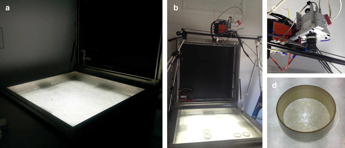
The tank's area of frozen ice is 0.85 m × 0.85 m and ice growth is initiated using 30 litres of filtered deionized water frozen overnight (at −20 °C) followed by the addition of 70 litres of pre-chilled (−1.7 °C) 0.2 µm filtered seawater. The initial addition of fresh water is necessary to ensure that the freezing seawater adhered to the base of the tank and did not float to the surface by expulsion of the hypersaline brine. The filtered seawater layer (36 ppt) was left to freeze for 2 days followed by the removal of excess hypersaline brine resulting in an ice thickness of ~70 mm. Additional pre-chilled seawater (−1.7 °C, 36 ppt) was then added to achieve a 20–30 mm water layer above the ice, which remained unfrozen at a temperature of ~−1.8°C. Images of the ice surface before algae inoculation are shown in Figures 2a, b.
(a) Image of the inverted sea-ice simulation tank in the dark room setting with all external light sources off. (b) Image of the inverted ice tank together with the motorized slider and the cylinder's set-up. (c) The SPECIM AISA Kestrel 10 hyperspectral imager. (d) High (H) algae abundance cylinder after two days of algae inoculation.
The upward directed light source is a Cree Xlamp XP-E High-Efficiency white LED and has a typical double bell spectral curve characteristic of white LED light sources (Fig. 1). It covers the Photosynthetically Active Radiation (PAR) (from 400 to 700 nm) range and provides moderate intensities in the regions of interest where ice algae show their main absorption peaks (e.g. Fritsen and others, Reference Fritsen, Wirthlin, Momberg, Lewis and Ackley2011). The lighting system was deliberately installed to be consistent with measured under-ice PAR irradiance intensities. For example, using a Li-COR PAR sensor to measure light flux at the ice/water interface of the inverted ice tank, we measured light levels ranging from 31.4 to 58.6 µmol photon m−2 s−1 from the dark areas to bright areas. This is comparable with in-situ measurements beneath Arctic (e.g. Lund-Hansen and others, Reference Lund-Hansen, Hawes, Sorrell and Nielsen2014) or Antarctic sea ice (e.g. SooHoo and others, Reference SooHoo1987). The glass sheet between the light source, the ice and water layers is optically clear allowing transmission of >90% of light and having minimal influence on the optical properties of the transmitted light.
Ice algae culturing and inoculation
Algal cultures consisting of Fragilariopsis cylindrus, Nitzschia stellata and Navicula glaciei were extracted from Antarctic sea ice in 2015, and maintained semi-continuously in L 10 media (Guillard and Ryther, Reference Guillard and Ryther1962) under cool white fluorescent light (60 µmol photon m−2 s−1, 12:12 light/dark cycle) at 2 ± 1°C. Each algal species was grown separately in a continuous batch system, bubbled with 0.2 um filtered air and amended with L 1 nutrients (Guillard and Ryther, Reference Guillard and Ryther1962). Before inoculation, cells were acclimated to −1°C over a 12-h period to limit any cold induced shock from the ice-tank environment. Once ready for inoculation, varying volumes were extracted from the parent cultures and added to a set of eight cylinders to spatially distribute algal biomass at increasing concentrations. This provided an increasing scale of biomass abundance intensities among the eight cylinders.
The cylinders were 80 mm in diameter and 50–60 mm high and were placed 20–30 mm deep in the ice layer and left emerging above the water surface layer (Fig. 2d). Two types of material were chosen for the cylinders; opaque PVC tubes and optically clear acrylic tubes. Based on the expected concentrations, the biomass abundance intensities inoculated in the eight cylinders were denominated as follows: two empty controls (C1 and C2) in PVC and acrylic, respectively; a Very Low (VL) in PVC; a Low (L) in acrylic; a Medium (M) in acrylic; a Medium High (MH) in PVC; a High (H) in acrylic; and a Very High (VH) in PVC. Figure 2d shows the VH PVC cylinder after inoculation.
Hyperspectral imaging
A pushbroom SPECIM AISA KESTREL 10 (AK10) hyperspectral line scanner was employed for imaging the algal distributions at the ice/water interface (Figs 2b, c). Imaging with the pushbroom sensor required a scan to be conducted in a forward motion across the target of interest in order to create the image (Fig. 1). Thus, the AK10 was integrated into a motorized slider with precise adjustable speeds for this purpose (Fig. 2b). The AK10 has a 40° Field of View (FOV) and comprises a total of 2048 pixels that can be binned into 1020 to improve the Signal to Noise Ratio (SNR) per pixel. The sensor's spectral range goes from 400 to 1000 nm and allows for customized spectral resolution and integration times (frequency) to be set according to the survey scenario. The motorized slider was placed 1.2 m above the ice/water interface (1 m considering the camera fore-optics) allowing the camera to achieve a spatial across-track resolution of 0.9 mm, which covered a scan line width of 728 mm. The imaging frequency was set to 5 Hz and the sliding rail speed ~8–10 mm s−1 providing along-track resolution of 0.8–0.9 mm (thus 0.9 mm square pixels in the composed image). Hereafter, a spatial resolution of 0.9 mm will refer to the 0.9 mm × 0.9 mm squared nature of the image pixel size. We selected the slider speed and frequency to maximize the intensity of the acquired signal, or SNR. For this experiment, we repeated the scanning process at three different spectral resolutions of 1.7, 3.4 and 6.8 nm in order to assess the effect of spectral resolution. All three frames were binned to 1020 pixels. The hyperspectral imaging was performed in the dark with no influence from any other external light source except the tank's LED light source (Fig. 2a). HI on the tank was performed 3 days after inoculation of algae.
Chl-a sampling
In order to provide a semi-quantitative validation of the six cylinders' chl-a concentrations, the cylinders were sampled using a 10 mL lab-pipette by scratching the ice while simultaneously sucking up any content at the ice/water interface in five different 1 cm2 random spots within each cylinder. 1 cm2 sample sub-areas were roughly measured with a mm-scale ruler resting above the cylinders while operating the pipette. The 50 mL samples for each cylinder were immediately filtered onto Whatman GF/F filters, extracted for 24 h in ethanol and analyzed for chl-a content according to Holm-Hansen and Riemann (Reference Holm-Hansen and Riemann1978) using a Turner 10 AU fluorometer.
Data processing
The images were composed from the acquired line-scans using SPECIM Lumo Recorder software. All hyperspectral images were converted to radiance values (W m−2 sr−1 nm−1) per pixel from the raw digital numbers (DN) using ENVI software and the provided calibration files. The images are then pre-processed using MATLAB. Pre-processing involved selecting a region of interest (ROI) and spectral filtering. Selecting an ROI was done manually and this process discarded the extra imaged areas that are not the ice/water interface such as the steel borders of the ice tank (Fig. 2b). Even though the images resulted in high SNR by measuring just below the saturation level, we performed a Savitzy-Golay filter with a third polynomial order and a filter width of five (Tsai and Philpot, Reference Tsai and Philpot1998; Vidal and Amigo, Reference Vidal and Amigo2012). The filter aimed to smooth out the high-frequency noise while preserving the relevant spectral features at low intensity wavelengths. In order to capture the differences between different algae abundances from light transmitted through the artificial sea ice, Principal Component Analysis (PCA) was performed on the three images taken at the three different spectral resolutions. The hyperspectral images consist of a three-dimensional (x, y, λ) data cubes where x and y represent the spatial dimension and λ the spectral dimension. PCA exploration method was applied in this case to track the most variable features across the spectral dimension of the hyperspectral images and to outline relevant spectral bands carrying the relevant information on ice-algal biomass (Rodarmel and Shan, Reference Rodarmel and Shan2002; Amigo and others, Reference Amigo, Babamoradi and Elcoroaristizabal2015).
Transmitted radiance measured with the AK10 was compared with publically available data from a series of Remotely Operated Vehicle (ROV) transects performed in the Arctic by Nicolaus and Katlein (Reference Nicolaus and Katlein2013) to provide a comparison with spectral data collected under in-situ conditions. Radiance along these transects, was measured using an ROV instrumented with a TRiOS RAMSES radiance sensor (of 3 nm spectral resolution). Operating depths ranged from 1 to 8 m, for different sea-ice types, which varied from snow-free to variable snow cover (from 2 to 10 cm thickness), from First Year Ice (FYI) to Multi Year Ice (MYI) (from 0.3 to 3.8 m thickness). Detailed information about each transect can be found in Nicolaus and Katlein (Reference Nicolaus and Katlein2013). The ROV dataset is available online under doi:10.1594/PANGAEA.78671.
RESULTS
The arrangement of the algal cylinders in the ice tank is shown in Figure 3a as an RGB composite image. The figure also displays the ice-algal biomass range from VL to VH as inoculated across the cylinders. The results of the PCA for the HI frame taken at 1.7 nm are shown in Figures 3b–d.
Results of PCA applied to the 1.7 nm spectral resolution frame of the ice surface. (a) RGB composite of the hyperspectral image after algae inoculation displaying the performed biomass redistribution among cylinders. The RGB composite image is similar to what is observable by the human eye or normal imagery. (b) First principal component (PC1) representing light intensity variability within the image. (c) PCA loadings for each of the principal components. Algae absorption bands are clearly visible in PC2 at ~450 and 680 nm. (d) Second principal component (PC2) representing algae biomass abundance variability. The colour bar is unit-less as representing PC intensities.
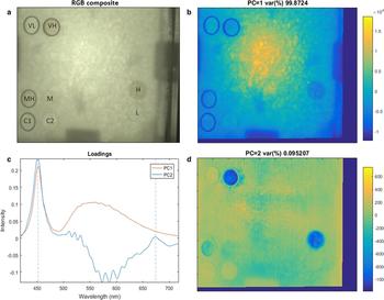
The first principal component (PC1) accounts for 99.8 % of the spectral variability (Fig. 3b) and represents variations in light intensity across the ice tank. This is confirmed by the loadings of PC1 that clearly match the spectral intensity of the LED light source (Figs 1, 3c). The light intensity is higher at the centre and decreases towards the edges of the ice tank. This difference in light intensity across the tank is mostly attributed to the non-diffuse (directional) light field emitted by the light source and the shadow structures in the image caused by the circulation fans and the presence of their sustaining structure between the light source and the ice. Another factor influencing light intensity variability was the different ice thickness observed from 7–9 cm at the centre to 5 cm at the edges (due to physical complications of achieving freezing conditions in those locations). PC1 does not contain any information regarding biomass variability but indicatively maps the light intensity distribution over the ice surface.
The second principal component (PC2) accounts for 0.09 % of the spectral variation in the hyperspectral image but displays a coherent relationship to the algal cylinder densities. High and low PC2 intensity areas match with low and high biomass values, respectively. Control cylinders (C1 and C2) stand out as high intensity areas opposing to H and VH cylinders (Fig. 3d). Results from the chl-a sampling are in agreement with the visual observations for VL (0.036 mg m−2), L (0.164 mg m−2), M (0.366 mg m−2), MH (0.636 mg m−2). Chl a sampling in cylinders H (2.712 mg m−2) and VH (1.804 mg m−2) did not match with the increasing inoculation scale with H cylinder having a higher chl-a concentration than VH. Loadings of PC2 in Figure 3c indicate that low PC2 intensity in Figure 3d is associated with increasing loading values at the peaks at ~450 and 680 nm (Fig. 3c). These peaks closely match with ice-algae absorption bands (Legendre and Gosselin, Reference Legendre and Gosselin1991; Fritsen and others, Reference Fritsen, Wirthlin, Momberg, Lewis and Ackley2011) suggesting a strong association between PC2 and ice-algal biomass. Within cylinder patchiness is also observed as darker spots of low PC2 intensity, particularly for cylinders MH, H and VH (Fig. 3d).
Loadings of PC2 are not purely representative of ice algae. Figure 3c shows that PC2 is also influenced by another element of variability affecting the spectral range between 500 and 650 nm. Opposite to ice algae, loadings on this component are low while algae related loading peaks (450 and 680 nm) are high. This high contrast can be observed at the edges of the PVC cylinders in Figure 3d thus suggesting that PC2 is influenced by variation caused by such cylinders and therefore slightly influencing the rest of the PC2 intensities across the image. This enhances PC2 intensity image features such as the shading of the circulation fans and the PVC cylinders themselves (Fig. 3d). Variability on the third principal component was also explored but did not show any relevant information.
The large disagreement between chl-a sampling in cylinder H and VH is attributed to leakage of algal-cells from cylinder VH to the surroundings as can be observed in Figure 3d at the top left. This leakage might have occurred during the hyperspectral image acquisition or later during chl-a sampling due to ice melting. Another cause might be the relatively poor efficacy of the chl-a sampling method compared with the within-cylinder variability for H and VH observed as dark spots spread across the 80 cm2 cylinder area (Fig. 2c).
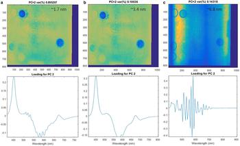
The analysis performed for the three different spectral resolutions (1.7, 3.4, 6.8 nm, respectively) demonstrates that while a spectral resolution of 3.4 nm is capable of performing the same differentiation as 1.7 nm, resolutions of >6 nm are not able to capture fine scale variability of biomass according to this first method exploration (Fig. 4). This is most likely related to the fine range of ice-algal spectral absorption features.
Principal component 2 (PC2) representing algae biomass variability for different spectral resolutions 1.7 nm (a), 3.4 nm (b), 6.8 nm (c), respectively. The difference in biomass PC2 loadings between 1.7 and 3.4 nm is minimal. The figure outlines the working spectral resolution range for hyperspectral imaging aimed to capture algae biomass abundance. The test suggests that sensors with spectral resolution above 6.8 nm cannot be used for the purpose and for example discards the use of snapshot hyperspectral sensors compared to pushbroom scanners. The colour bar is omitted.
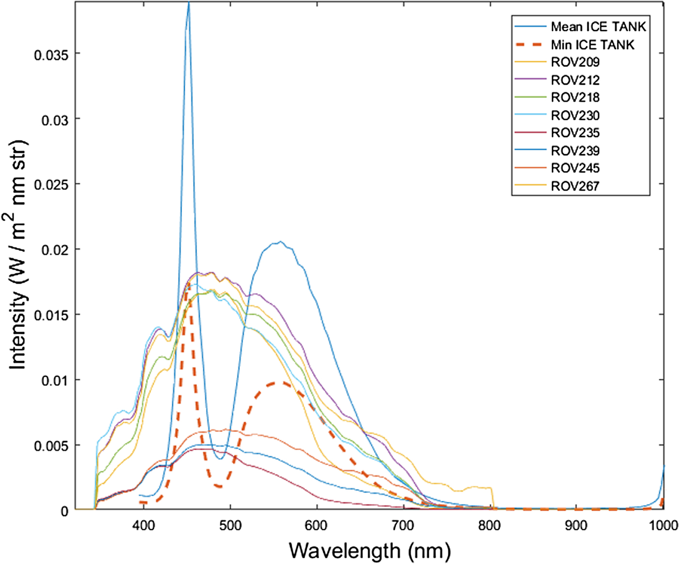
The AK10 measured radiance per pixel across the tank. It is observed that radiance intensities measured in the tank are in the same spectral radiance range compared with the measurements by Nicolaus and Katlein (Reference Nicolaus and Katlein2013) across different types of sea-ice conditions and ROV depths (Fig. 5). The ROV transects numbers are chosen as indexed in the original dataset (Nicolaus and Katlein, Reference Nicolaus and Katlein2013).
Comparison of radiance levels measured in the inverted ice tank with a series of Arctic under-ice radiance transects measured in-situ with a Remotely Operated Vehicle (ROV) for different sea-ice conditions. The ice tank radiance is obtained from the hyperspectral frames. Mean ICE TANK is the mean between all pixels in the frame whereas Min ICE TANK is the pixel with minimum intensity (taken in a non-shadowed area). ROV transects data are publicly available from the study performed by Nicolaus and Katlein (Reference Nicolaus and Katlein2013) in Arctic sea ice. Sea-ice conditions varied from snow to no snow cover (from 2 to 10 cm thickness), from First Year Ice (FYI) to Multi Year Ice (MYI) (from 0.3 to 3.8 m thickness) and ROV water depth varied from 1 to 8 m.
DISCUSSION
In this study, we present the first results of a laboratory experiment employing an HI camera for differentiating ice-algae biomass distribution at the ice/water interface. Employing a sliding pushbroom hyperspectral sensor over an inverted sea-ice tank allows to test the ability of hyperspectral imaging for capturing the detailed spatial distribution of sea-ice algae and test a range of hyperspectral sensor configurations, such as spectral resolution and integration time.
Sea ice is a three phase medium (principally consisting of ice, brine and air bubbles) with high scattering properties and contains optically active substances in the PAR range such as Colored Dissolved Organic Matter (CDOM) but in particular microalgae (Perovich, Reference Perovich1996; Grenfell and others, Reference Grenfell, Light and Perovich2006; Xie and others, Reference Xie, Aubry, Zhang and Song2014). Light reaching the ice sub-surface can be reduced to <1% of the incoming solar radiation depending on surface and ice properties (e.g. due to snow, presence of melt-ponds, ice thickness, ice structure, etc.) resulting in very low under-ice light levels (Petrich and others, Reference Petrich, Nicolaus and Gradinger2012). Sea ice also affects the geometric properties of the light field exiting the medium due to its lamellar structure funnelling light in a downward direction and generating a forward peaked light field (Katlein and others, Reference Katlein, Nicolaus and Petrich2014).
We have presented a proof of concept study conducted under controlled laboratory conditions to test HI technology as a new remote-sensing technique to map ice algal distribution at the bottom of the sea ice. The hyperspectral frames acquired with a 0.9 mm square pixel spatial resolution and spectral resolutions of 1.7 and 3.4 nm were able to provide spectral differentiation between different algal concentrations at the ice/water interface in our experimental set-up. The results were validated by the pre-determined cylinder inoculation scale and chl-a sampling within the cylinders. It is noted that our chl-a measurements do not provide an exact determination of chl-a within the cylinders but serve as a semi-quantitative measure of the algal biomass to allow for between cylinder comparison.
Spectral resolutions >6 nm were not able to provide such discrimination due to the finer spectral scale of algae absorption features compared with the coarser transmitted light curve measured. This result has further importance in selecting appropriate sensors for this detection of ice algae. For example, snapshot hyperspectral sensors are easier to use (more portable and not constantly requiring six orientation parameters) than pushbroom sensors, which require constant and accurate forward motion and are sensitive to drift. However, to attain adequate SNR and due to the finite number of pixels on a focal plane array, snapshot HI sensors necessarily make a trade-off in the resolution of the various dimensions of data of the hypercube sacrificing either spatial or spectral resolution. Considering the low-light of the under-ice environment, the high micro-scale spatial variability of ice algae and its fine-scale spectral features, snapshot HI would be very limited in this type of application.
Comparison of the experimental set-up with an in-situ scenario
It might be argued that light intensity measured in the ice tank is different from the typically low intensity transmitted solar radiation found under sea ice. Thus, the capability of a HI sensor to perform in low light conditions in a dynamic setting would be put into question. The effect of increasing distances from the sensor to the sea-ice bottom (water-column thickness) would further accentuate this issue. Our study compared measured radiance intensity levels with the AK10 to multiple in-situ situations showing consistent light levels even for the worst case scenarios around algae absorption bands (690 nm) (Fig. 5). Additionally, the measurements maximized the SNR by reaching near saturation light levels. We expect that with the same settings, lower light levels would affect SNR but would still yield accurate information on algae spatial distribution.
The different spectral signature of the LED light source compared with sunlight radiation is not expected to influence PCA results in an in-situ scenario. The spectral bands representing algae variability are quite narrow (as seen in PC2 loadings in Fig. 3c), and PCA was capable of decomposing between the spectral composition of the light source (with variability due to changes in overall intensity, as PC1) and algae related absorption bands (as PC2). Lange and others (Reference Lange, Katlein, Nicolaus, Peeken and Flores2016) observed a similar behaviour in-situ when employing Empirical Orthogonal Functions (EOFs) (analogous to PCA) outlining how secondary modes (or PCs) are free of the dominant signal spectral variability and better represent chl-a absorption.
A similar ice structure to that found in the field, with lamellar ice crystals, brine and air pockets, was also observed within the ice tank (using macro photography). This caused the light to be in a diffuse and scattered form similar to in-situ observations (Petrich and others, Reference Petrich, Nicolaus and Gradinger2012). The spatial variability of light intensity caused by the lamp and variations in the ice thickness is not considered disadvantageous. Snow is the most common and greatest attenuator of light in the snow – sea-ice layered matrix and produces a similar effect creating high variability in light intensities within very short distances (e.g. Nicolaus and others, Reference Nicolaus, Petrich, Hudson and Granskog2013). Indeed, our experimental results suggest the method's indifference to light intensity variability (e.g. induced by spatially variable snow and ice thickness). This observation would need to be further investigated for a real sea-ice sampling scenario that comprises additional optically active elements. However, our results outline the potential of the technique to focus only on relevant spectral features associated with sea-ice algae presence and biomass variability. From an optical HI perspective, the experimental set-up therefore properly represented the four components of the layered structure of real sea ice (air, ice, water, algae). Whether it will be possible to control and mimic natural ice features including the skeletal layer and quantify columnar ice growth, are considerations for future experiments.
Ice algae were inoculated 3 days prior to the imaging in the ice tank and resided at the ice/water interface only (~5 mm deep in the ice structure). While measured chl-a concentrations are proportional to in-situ observations both in the Arctic (Arrigo and others, Reference Arrigo, Mock, Lizotte, Thomas and Dieckmann2010) and the Antarctic (Meiners and others, Reference Meiners2012), depending on the region, in-situ ice-algae concentrations might be vertically variable (Meiners and others, Reference Meiners2012; Arrigo, Reference Arrigo2014). Notwithstanding, higher concentrations of sea-ice algae are most frequently found in the bottom <10 cm of the ice, and can also be found exclusively attached at the ice/water interface (Arrigo, Reference Arrigo2014; Lund-Hansen and others, Reference Lund-Hansen, Hawes, Nielsen and Sorrell2016). Another consideration in interpreting the spectral data is the physiological status of the algal cultures. All three cultures were in an exponential growth phase prior to inoculation and acclimated to 60 µmol photon m−2 s−1, which was a comparable irradiance with that provided by the ice tank. In natural conditions, sea-ice algae can be exposed to different levels of irradiance and can respond physiologically to these changes. For example, shade-adaptation requires that intracellular chlorophyll a is upregulated to maximize the capacity for growth and different compounds of accessory pigments can be produced under different irradiance conditions (SooHoo and others, Reference SooHoo1987; Fritsen and others, Reference Fritsen, Wirthlin, Momberg, Lewis and Ackley2011). In an in-situ scenario, this and other biological components of the within-ice community (dead algae cells and detritus) are likely to influence the spectral signatures observed with HI sensors by slightly shifting the spectral bands better representing algae variability in PCA analysis.
A new type of vision under the ice: possibilities, limitations and future work
The main advantage of the proposed application of HI is the ability to capture light at high spectral and spatial resolutions (in this case mm scales) in a non-invasive manner with great potential for studies aimed at investigating ice-algal spatial distribution, variability and environmental controls (Campbell and others, Reference Campbell, Mundy, Barber and Gosselin2015; Lange and others, Reference Lange, Katlein, Nicolaus, Peeken and Flores2016; Lund-Hansen and others, Reference Lund-Hansen, Hawes, Nielsen and Sorrell2016). Studies employing hyperspectral imaging for different types of underwater biomes have been performed on mycrophytobenthos (Chennu and others, Reference Chennu2013) and coral reef biota (Caras and Karnieli, Reference Caras and Karnieli2015).
By establishing local in-situ correlations between chl-a and spectral indices such as NDIs (Melbourne-Thomas and others, Reference Melbourne-Thomas2015) or EOFs (Lange and others, Reference Lange, Katlein, Nicolaus, Peeken and Flores2016) the hyperspectral image processing workflow can then be theoretically extended to regression analysis and quantification of chl-a per pixel unit. Planned future work will investigate the possibility of applying different statistical approaches to the acquired imagery.
In the present tests, HI frames captured radiance at mm resolution but biomass differences were only validated among the cylinders. Variability in PC2 intensity was observed across the rest of the entire ice tank (outside of the cylinders) probably due to the random inoculation. Nevertheless, we cannot prove that these fine-scale intensity variations are associated with fine-scale (sub-millimetre) patterns in algal spatial distribution. Even though we visually observed a leakage pattern in PC2 at sub-millimetre resolution from a cylinder (Fig. 3d), at this stage we are not able to quantitatively validate this due to the difficulty of sampling chl-a at such small scales.
Different scanning distances from the ice surface can yield different HI spatial resolutions ranging from sub-millimetre to the meter scale. Employing the sensor at increased distances from the ice sub-surface would allow to scan and map higher spatial extents at the cost of spatial resolution. However, influences caused by the anisotropic properties of the under-ice light field need to be carefully taken into consideration when measuring radiance from multiple angular directions such as the ones obtained from a large FOV HI sensor (Katlein and others, Reference Katlein, Perovich and Nicolaus2016, Reference Katlein, Nicolaus and Petrich2014). Water column correction would also need to be considered and corrected for, if greater surveying depths are to be considered (Johnsen and others, Reference Johnsen2013).
The use of close-range hyperspectral imaging is an emerging area of study with technical challenges to overcome for marine applications. In the marine environment, technical challenges are often accentuated for spectral analysis and sensor deployment. In the under-ice environment we are faced with further limitations such as selecting an appropriate material for the camera housing that maintains its optical integrity and can operate under very low temperatures. To the authors knowledge, only a few published studies are currently available on deploying hyperspectral imaging cameras under water, but the technology certainly presents great potential from a marine remote-sensing perspective (Chennu and others, Reference Chennu2013; Johnsen and others, Reference Johnsen2013).
HI systems could theoretically be deployed on Autonomous Underwater Vehicles or ROVs (Johnsen and others, Reference Johnsen2013). In the present test, we employed a stable and relatively accurate motorized slider moving at slow speeds (8–10 mm s−1) and relatively low frequency (5 Hz). Much more investigation is required for assessing HI systems performance on an underwater vehicle of any kind.
CONCLUSION
Current biomass sampling methodologies are not capable of capturing the abundance and distribution of sea-ice algae. Therefore, little is known of how changes in their environment will affect their existence with concomitant impacts on the whole marine polar food web and high latitude carbon cycles.
Through an experimental set-up consisting of an ‘inverted’ sea-ice simulation tank we were able to map transmitted light through an algal-colonized sea-ice layer at unprecedented spectral (1.7, 3.4 and 6.8 nm) and spatial resolutions (0.9 mm square pixel size). Decomposition of the hyperspectral data through PCA outlined two main components of variability in the images; the first (PC1) representing light intensity and the second (PC2) representing algae biomass across the tank. Light intensity variability is typically found in the field and is mostly attributed to variations in snow thickness. Biomass abundance in-situ is mostly concentrated at the bottom of the ice at the ice/water interface with algae presenting multiple degrees of ‘patchiness’. Overall, the inverted sea-ice simulation tank presented an adequate optical set-up for investigating the application of hyperspectral imaging (HI) cameras for ice-algal studies.
In this preliminary experiment, HI was able to differentiate between low and high biomass abundances and was validated over a discrete scale of six cylinder units with increasing concentrations. Further observations, such as within-cylinder patchiness and algae leakage from a cylinder observed in the PCA analysis plots, suggested the ability to discriminate algae variability at cm to mm scale. Our assessment of three different spectral resolutions indicated that while bandwidths of 1.7 and 3.6 nm successfully captured algae biomass spatial variability, bandwidths over 6 nm were not provide such differentiation. This suggests that a sensible sensor configuration is required for ice-algal habitat mapping.
Planned future work will investigate several aspects aimed to move towards the deployment of the technology in-situ by assessing varying spatial resolutions, varying light intensity levels, varying camera settings (such as movement speed and imaging frequency) and applying regression models to correlate hyperspectral imagery data to sampled chl-a values among others. Further investigation in HI technology is also required for assessing the range of spatial resolutions achievable for capturing the multiple spatial scales of variability of ice-associated algae, and for the potential of characterizing under-ice light field properties, as seen in the PC1 light intensity distribution mapping (Katlein and others, Reference Katlein, Perovich and Nicolaus2016, Reference Katlein, Nicolaus and Petrich2014). The methodology proposed in this study is still in its infancy with several important caveats that need to be addressed. Nevertheless, this study demonstrates the potential of hyperspectral imaging as an improved and valid methodology capable of providing unprecedented datasets for estimating sea-ice algal biomass at the ice/water interface.
ACKNOWLEDGEMENTS
This research was supported under Australian Research Council's Special Research Initiative for Antarctic Gateway Partnership (Project ID SR140300001). We acknowledge the University of Tasmania Terraluma's group and Terraluma engineer Richard Ballard for advice and technical support. We gratefully acknowledge the collaboration with Petri Nygrén from SPECIM (Spectral Imaging Ltd) and Marc Fimeri (Adept Turnkey Pty Ltd) for assisting with the collection of the hyperspectral imagery and laboratory testing with the AISA KESTREL 10. Emiliano Cimoli is supported by the Antarctic Gateway Partnership and the University of Tasmania's PhD program.


 Open access