







Impact Statement
This paper applies machine learning and explainable AI to identify how environmental drivers shape net ecosystem exchange (NEE) in boreal and hemiboreal forests. By pairing predictive models with transparent explanations, we target the variables and interactions that matter most for carbon uptake and release. Particular attention is paid to diffuse radiation, which can enhance photosynthesis via the diffuse fertilization effect, yet the impact of diffuse radiation is difficult to separate from the impact of other variables. Here we offer a new ML-based insight into this challenge, which is based on SHapley Additive exPlnations (SHAP). The additivity of SHAP contributions allows for quantifying how much different variables contribute to NEE at a given time. In doing so, we contribute methodologically by demonstrating SHAP as a tool for ecosystem process analysis and ecologically by providing cross-site quantification of how diffuse radiation and its interactions relate to NEE.
1. Introduction
Forests play a crucial role in the global carbon cycle by removing atmospheric carbon dioxide through photosynthesis and storing it in wood biomass and forest soils. Recent studies indicate that while carbon uptake has declined in tropical forests over the past few decades, it has increased significantly in boreal forests, which are now recognized as the largest terrestrial carbon sink globally (Tagesson et al., Reference Tagesson, Schurgers, Horion, Ciais, Tian, Brandt, Ahlström, Wigneron, Ardö, Olin, Fan, Wu and Fensholt2020). Although the basic mechanisms of forest carbon cycling and their climatic drivers are broadly understood, disentangling how different factors contribute to net ecosystem exchange (NEE) is critical given their strong co-variation, nonlinear responses, and interactions.
Central to forest climate impacts is gross primary productivity (GPP), which represents carbon uptake via photosynthesis, and ecosystem respiration, which represents carbon release. These two fluxes combined give NEE. The eddy-covariance technique is commonly used to measure NEE, from which GPP can then be estimated indirectly by subtracting respiration from the observed NEE. Measurements of NEE are essential, as variations in net carbon exchange directly influence regional and global carbon budgets. They are used to study interactions between terrestrial ecosystems and climate, aiding vegetation and climate model validation and regional carbon budgeting (Zhou et al., Reference Zhou, Yue, Lei, Tian, Ma and Cao2021a). Eddy-covariance measurements are subject to known uncertainties, such as systematic biases, sensor limitations, and footprint-related scaling issues, which often necessitate gap filling to obtain continuous turbulent-flux records (Richardson et al., Reference Richardson, Hollinger, Burba, Davis, Flanagan, Katul, Munger, Ricciuto, Stoy, Suyker, Verma and Wofsy2006; Khan et al., Reference Khan, Liaqat, Baik and Choi2018).
Solar radiation significantly influences ecosystem photosynthesis, thereby affecting NEE directly (Zhou et al. Reference Zhou, Yue, Lei, Zhang, Tian, Ma and Cao2021b). Radiation includes direct and diffuse components, with diffuse radiation, enhanced by clouds and aerosols, being particularly important due to its ability to penetrate deeper and more evenly into forest canopies (Ezhova et al., Reference Ezhova, Ylivinkka, Kuusk, Komsaare, Vana, Krasnova, Noe, Arshinov, Belan, Park, Lavric, Heimann, Petäjä, Vesala, Mammarella, Kolari, Bäck, Rannik, Kerminen and Kulmala2018). Observations have confirmed the substantial influence of diffuse radiation on NEE, GPP, and ecosystem light-use efficiency (LUE) under varying atmospheric conditions (Mercado et al., Reference Mercado, Bellouin, Sitch, Boucher, Huntingford, Wild and Cox2009; Ezhova et al., Reference Ezhova, Ylivinkka, Kuusk, Komsaare, Vana, Krasnova, Noe, Arshinov, Belan, Park, Lavric, Heimann, Petäjä, Vesala, Mammarella, Kolari, Bäck, Rannik, Kerminen and Kulmala2018; Neimane-Šroma et al., Reference Neimane-Šroma, Durand, Lintunen, Aalto and Robson2024). Accordingly, failing to model diffuse radiation properly can cause modeling efforts to fail at predicting carbon uptake at sites. For example, Yuan et al. (Reference Yuan, Cai, Xia, Chen, Liu, Dong, Merbold, Law, Arain, Beringer, Bernhofer, Black, Blanken, Cescatti, Chen, Francois, Gianelle, Janssens, Jung, Kato, Kiely, Liu, Marcolla, Montagnani, Raschi, Roupsard, Varlagin and Wohlfahrt2014) used seven LUE-based GPP models and found that six of them severely underestimated the observed GPP under overcast skies due to neglecting diffuse radiation. Another study found that in northern China’s croplands and forests, failing to include changing diffuse radiation led LUE-model estimates to understate the observed trend in GPP, as the aerosol pollution in that region increased diffuse light and boosted plant productivity (Liu et al., Reference Liu, Tong, Zhang, Meng, Li, Zhang and Zhou2022). These cases emphasize the fact that diffuse radiation is critical for accurately modeling carbon uptake, especially in boreal forests, where the GPP seems to increase more in response to diffuse radiation than in other ecosystems (Zhou et al. Reference Zhou, Yue, Lei, Zhang, Tian, Ma and Cao2021b).
To further enhance the understanding and prediction of ecosystem carbon fluxes and their responses to solar radiation conditions, machine learning (ML) techniques have increasingly complemented traditional process-based modeling approaches (Launiainen et al., Reference Launiainen, Katul, Leppä, Kolari, Aslan, Grönholm, Korhonen, Mammarella and Vesala2022; Junttila et al., Reference Junttila, Minunno, Peltoniemi, Forsius, Akujärvi, Ojanen and Mäkelä2023). ML models provide flexible, empirical alternatives to traditional hypothesis-driven (deductive) models by directly relating input variables to carbon flux outcomes, including NEE. Such ML models have demonstrated strong predictive performance in estimating carbon cycle variables from data-driven perspectives, broadening the analytical toolkit available to researchers (Cai et al., Reference Cai, Xu, Zhu, Hu and Li2020; Zeng et al., Reference Zeng, Matsunaga, Tan, Saigusa, Shirai, Tang, Peng and Fukuda2020; Zhu et al., Reference Zhu, Yu, Chen, Zhang, Han, Wang, Chen, Liu, Wang, Yan, Tan, Zhang, Zhao, Li, Zhang, Shi, Zhu, Wu, Zhao, Hao, Sha, Zhang, Jiang, Gu, Wu, Zhang, Zhou, Tang, Jia, Li, Song, Dong, Gao, Jiang, Sun, Wang, He, Li, Wang, Wei, Deng, Hao, Li, Liu, Zhang and Zhu2023).
Nevertheless, modern ML models often behave as black boxes, making it difficult to see how input data influence predictions. Results should, therefore, be interpreted with care, and evaluation should go beyond a single metric, as aggregate scores can hide failure modes, biases across subgroups (e.g., sites, seasons), and misleading correlations. Explainable AI (XAI) methods address this gap by attributing predictions to input variables and summarizing effects across the dataset, improving transparency and model critique. Integrating XAI with ML clarifies when and why models succeed or fail, reveals potential biases, and improves communication, yielding deeper insight (Dwivedi et al., Reference Dwivedi, Dave, Naik, Singhal, Omer, Patel, Qian, Wen, Shah and Morgan2023).
In this study, we model NEE at sub-hourly resolution in boreal and hemiboreal forests, using input datasets from three research stations located at different latitudes: Värriö (67°46’ N), Hyytiälä (61°51’ N), and Järvselja (58°16’ N). This multi-site approach captures latitudinal variation in carbon dynamics. Our central focus is the role of diffuse radiation in shaping NEE, while accounting for other environmental drivers. We assess how model complexity influences predictive performance and variable relationships by comparing two input variable configurations: a reduced setup utilizing only four critical variables and a full configuration using 10 variables. These analyses are carried out with three different ML models, enabling us to compare not only variable sets but also how different modeling approaches capture the drivers of NEE.
To improve interpretability and reveal underlying ecological processes, we apply the XAI method SHAP (SHapley Additive exPlanations). SHAP provides model-agnostic, per-instance attributions (positive/negative relative to a baseline) and scalable global summaries, and its dependence plots expose context-dependent interactions among predictors. We compute SHAP values for each sub-hourly data point to quantify variable contributions to NEE at the time-step level, rather than relying solely on global effects as in our previous work (Ezhova et al. Reference Ezhova, Laanti, Lintunen, Kolari, Nieminen, Mammarella, Heljanko and Kulmala2025a). Using these tools, we highlight the role of diffuse radiation across seasons and model configurations.
Our goals are to:
-
1. Identify the environmental drivers that best explain full-season, hourly NEE dynamics across boreal and hemiboreal forests spanning 58–67°N.
-
2. Quantify how these drivers affect NEE as inferred by three machine-learning models and SHAP, and assess the consistency of attributions across models.
-
3. Evaluate how diffuse radiation affects NEE by comparing conventional threshold-based grouping with SHAP-based stratification (DiffPAR SHAP grouping).
Through this approach, we aim to deepen understanding of diffuse radiation’s role in boreal carbon fluxes while demonstrating how explainable ML can be used not only for attribution but also for process-relevant stratification of ecosystem states.
2. Materials and methods
2.1. Data
We used atmospheric observations from three distinct measuring stations: SMEAR I Station in Värriö, Finland (Hari et al., Reference Hari, Kulmala, Pohja, Lahti, Siivola, Palva, Aalto, Hämeri, Vesala, Luoma and Pulliainen1994), SMEAR II in Hyytiälä, Finland (Hari and Kulmala, Reference Hari and Kulmala2005), and SMEAR Estonia in Järvselja, Estonia (Noe et al., Reference Noe, Niinemets, Krasnova, Krasnov, Motallebi, Kängsepp, Jõgiste, Hõrrak, Komsaare and Mirme2015). SMEAR stands for Station for Measuring Ecosystem-Atmosphere Relations, and the focus of SMEAR stations is comprehensive long-term measurements of the ecosystem–atmosphere interactions. Each site measures carbon fluxes and various meteorological variables as well as radiation. All the sites operate with similar instrumentation, and the observation sites are briefly described below.
The SMEAR I station is located in Värriö in a boreal forest that grows on mineral soil in Northern Finland (67°46’N, 29°36’E, 180 m a.s.l.), with a mean annual air temperature of −0.5°C and a mean annual precipitation of 601 mm. Värriö forest is dominated by 70-year-old Scots pines ( Pinus sylvestris L.) that have an average tree height of 10 m, measured in 2023, with an open forest canopy. For more details on the SMEAR I station, please refer to (Hari et al., Reference Hari, Kulmala, Pohja, Lahti, Siivola, Palva, Aalto, Hämeri, Vesala, Luoma and Pulliainen1994; Duplissy et al., Reference Duplissy, Väänänen, Kerminen, Virkkula, Petäjä, Asmi, Dal Maso, Nieminen, Juhola, Shcherbinin, Riipinen, Lehtipalo, Keronen, Aalto, Hari and Kulmala2014; Vana et al., Reference Vana, Komsaare, Hõrrak, Mirme, Nieminen, Kontkanen, Manninen, Petäjä, Noe and Kulmala2016).
The SMEAR II station is located in Hyytiälä in a boreal forest on mineral soil in central Finland (61°51’N, 24°17’E, 80 m a.s.l.) with a mean annual air temperature of 3.5°C and a mean annual precipitation of 710 mm. Hyytiälä forest stands are dominated by 63-year-old Scots pines (P. sylvestris L.) that have an average tree height of ca. 19.9 m, as measured in 2023. The forest canopy was closed until the thinning of the forest in 2020. A detailed overview of the site and the measurements can be found in (Hari et al., Reference Hari, Nikinmaa, Pohja, Siivola, Bäck, Vesala, Kulmala, Hari, Heliövaara and Kulmala2013).
Järvselja station is located in the southern transition zone of the boreal biome, the hemiboreal forest (58.2714 N, 27.2703 E, 36 m a.s.l.), with a mean annual temperature of 4–6°C and a mean annual precipitation of 500–750 mm. The forest is dominated by birch species (Betula pendula Roth, B. pubescens Ehrh.) or co-dominated with Scots pine (P. sylvestris L.) and Norway spruce ( Picea abies (L.) Karst.) that have an average tree height of 25 m. The forest canopy is closed. A detailed overview of the site and measurements can be found in (Noe et al., Reference Noe, Niinemets, Krasnova, Krasnov, Motallebi, Kängsepp, Jõgiste, Hõrrak, Komsaare and Mirme2015).
All three sites are part of the Integrated Carbon Observation System (ICOS) as well as the Aerosol, Clouds and Trace Gases Research Infrastructure (ACTRIS), while Värriö and Hyytiälä sites are also part of the Integrated European Long-Term Ecosystem, Critical Zone, and Socio-Ecological Research (eLTER) networks. For SMEAR I and SMEAR II, the data are publicly available from the SmartSMEAR Database (https://smear.avaa.csc.fi/), accessed in September 2022; the latest updated data sets can be found at https://etsin.fairdata.fi/data%20sets/SmartSMEAR.
The data used in this study were collected at a 30-minute measurement interval. The high frequency allows the study of the daily cycle of NEE, as well as the impact of variables affecting the ecosystem on a short time scale. The target variable, NEE, is formed by data on CO
$ {}_2 $
 fluxes with the eddy covariance technique (Aubinet et al., Reference Aubinet, Vesala and Papale2012) and then processed into NEE using the EddyUH software (Mammarella et al., Reference Mammarella, Peltola, Nordbo, Järvi and Rannik2016). Negative NEE corresponds to the ecosystem acting as a net carbon sink, while positive NEE corresponds to the ecosystem acting as a net carbon source.
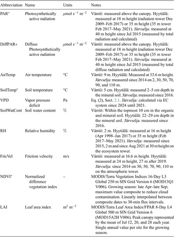
We modeled NEE using meteorological variables, with the full list provided in Table 1, and their distributions shown as boxplots in Supplementary Figure A1. The data used were non-gap-filled to avoid the influence of models used in gap-filling. For some of the input variables, there existed minor differences in how the data were measured at the three different stations; for example, soil moisture was measured from different depths. At Hyytiälä, PAR was not measured before 2009, and we used global radiation multiplied by the PAR quantum efficiency of 2
$ \mu $
 mol s
$ {}^{-1} $
mol s
$ {}^{-1} $
 W
$ {}^{-1} $
W
$ {}^{-1} $
 (Ross and Sulev, Reference Ross and Sulev2000; Ezhova et al., Reference Ezhova, Ylivinkka, Kuusk, Komsaare, Vana, Krasnova, Noe, Arshinov, Belan, Park, Lavric, Heimann, Petäjä, Vesala, Mammarella, Kolari, Bäck, Rannik, Kerminen and Kulmala2018) to calculate missing values of PAR. The amount of points used is listed in Table 2. Regarding satellite data, we used MODIS-derived vegetation indices covering the period 2000–2022, specifically the MODIS/Terra Vegetation Indices 16-Day L3 Global 250 m SIN Grid Version 6 (MOD13Q1 V006) for NDVI and the MODIS/Terra Leaf Area Index/FPAR 8-Day L4 Global 500 m SIN Grid Version 6 (MOD15A2H V006) for LAI. NDVI was extracted at 250 m spatial resolution for the growing season, defined as the period from the end of April to the end of September, using the 16-day clear-sky composite product. To reduce cloud contamination, we applied a maximum value composite (MVC) approach. For LAI, we used 500 m resolution data and calculated the average of three MODIS acquisition dates—July 12, 20, and 28—to represent peak canopy development during the growing season. These dates were selected to capture the period of maximum leaf area and productivity, consistent with common practices in seasonal vegetation monitoring.
List of input variables used for model training
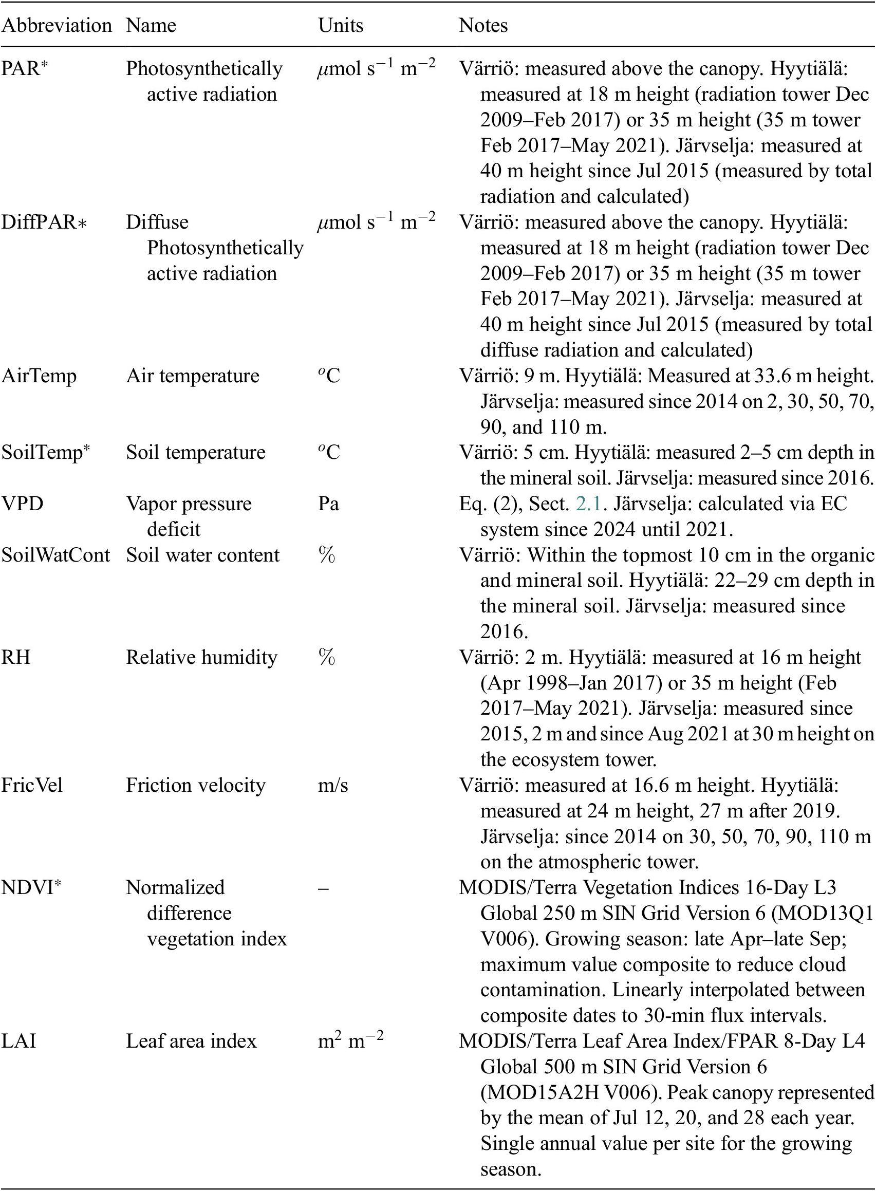
Table 1. Long description
The table contains four columns: Abbreviation, Name, Units, and Notes.
* P A R asterisk: Photosynthetically active radiation. Units: micromoles per second per square meter. Notes: Measured above canopy at Värriö, 18 to 35 m at Hyytiälä, and 40 m at Järvselja.
* Diff P A R: Diffuse P A R asterisk. Units: micromoles per second per square meter. Notes: Similar measurement heights to P A R.
* AirTemp: Air temperature. Units: degrees Celsius. Notes: Measured at 9 m at Värriö, 33.6 m at Hyytiälä, and multiple heights up to 110 m at Järvselja.
* SoilTemp asterisk: Soil temperature. Units: degrees Celsius. Notes: Measured at 5 cm depth at Värriö and 2 to 5 cm at Hyytiälä.
* V P D: Vapor pressure deficit. Units: Pa. Notes: Calculated via E C system.
* SoilWatCont: Soil water content. Units: percent. Notes: Measured in topmost 10 cm at Värriö and 22 to 29 cm at Hyytiälä.
* R H: Relative humidity. Units: percent. Notes: Measured at 2 m at Värriö, 16 to 35 m at Hyytiälä, and 2 to 30 m at Järvselja.
* FricVel: Friction velocity. Units: meters per second. Notes: Measured at 16.6 m at Värriö, 24 to 27 m at Hyytiälä, and up to 110 m at Järvselja.
* N D V I asterisk: Normalized difference vegetation index. Units: none. Notes: Derived from M O D I S slash Terra satellite data at 250 m resolution.
* L A I: Leaf area index. Units: meter squared per meter squared. Notes: Derived from M O D I S slash Terra satellite data at 500 m resolution.
Note: Variables marked with an asterisk are used when training models with only four variables.
Note. Input variables marked with an asterisk * are the variables used when training the models with only four variables.
Note. This table provides a list of input variables used for model training.
Summary of data sets: time periods and number of observations

Table 2. Long description
The table consists of three columns titled Site and case, Dates, and N obs.
Row 1: Hyytiälä, 07 forward slash 2008 to 09 forward slash 2018, 50,786 observations.
Row 2: Värriö, 05 forward slash 2013 to 10 forward slash 2019, 26,142 observations.
Row 3: Järvselja, 04 forward slash 2016 to 12 forward slash 2018, 7,882 observations.
Note. This table summarizes the time periods and number of observations for different data sets.
The data were pre-processed. Time points that contained missing values for any studied input variable were discarded, with some exceptions. To temporally align the NDVI time series with the 30-minute flux data, we performed gap-filling using simple linear interpolation between the 16-day composite values. All rows where PAR was less than 10
$ \mu $
 mol s
$ {}^{-1} $
mol s
$ {}^{-1} $
 m
$ {}^{-2} $
m
$ {}^{-2} $
 were filtered out, as the focus was solely on modeling daytime NEE.
Vapor pressure deficit (VPD) was calculated from air temperature (
$ {T}_{air} $
 ) and relative humidity (RH) as follows:
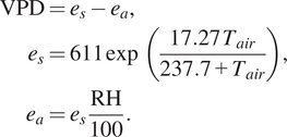
Here,
$ {T}_{air} $
 is the air temperature [°C], RH is the relative humidity [%],
$ {e}_s $
is the air temperature [°C], RH is the relative humidity [%],
$ {e}_s $
 is the saturation vapor pressure [Pa], and
$ {e}_a $
is the saturation vapor pressure [Pa], and
$ {e}_a $
 is the actual vapor pressure [Pa].
2.2. Machine Learning models
Following data preprocessing, we trained ML models to predict NEE based on meteorological, radiation, and vegetation-related variables. To capture both the non-linear interactions and potential regional variability in NEE drivers, we selected three widely used and high-performing algorithms for tabular data: XGBoost (Chen and Guestrin, Reference Chen and Guestrin2016), Light Gradient Boosting Machine (LightGBM) (Ke et al., Reference Ke, Meng, Finley, Wang, Chen, Ma, Ye and Liu2017), and Random Forest (Breiman, Reference Breiman2001).
This ensemble of models allowed us to assess not only predictive performance but also the consistency of variable importance across different modeling approaches. By comparing the explainability results of these models, we assessed whether the SHAP-based explanations (discussed in the following section) remained consistent across the different ML model architectures. If key variables consistently emerged as influential across the different ML models, we could be more confident that these patterns reflected underlying ecological processes rather than artifacts of a specific algorithm.
All models were implemented in R (v. 4.4.0: https://www.r-project.org/, last access: November 2024) using the tidymodels framework (v. 1.2.0: https://github.com/tidymodels/tidymodels, last access: November 2024).
2.2.1. Experimental setup
To train and evaluate the models, we split each site’s data into 75% training and 25% test sets using stratified sampling to preserve the full range of extremes. Although sample sizes differed by site, constructing a balanced dataset did not improve predictive performance overall or per site (Ezhova et al., Reference Ezhova, Laanti, Lintunen, Kolari, Nieminen, Mammarella, Heljanko and Kulmala2025a). We also trained models without explicit site labels, confirming that patterns were consistent across datasets while retaining a wider spectrum of environmental variability. Pooling the data from all sites increased sample size and diversity, which improved generalization and reduced overfitting to site-specific differences. This also strengthened the reliability of the resulting feature attributions.
In addition, we developed two sets of models to assess the consistency of the relationships between the input variables and NEE. One model configuration was trained using only the four input variables marked in Table 1, referred to as the reduced input set. We defined the reduced input set as the four top-ranked variables by mean absolute SHAP value from a model trained on the full input set, which contains all the variables (Section 3.2). This dual-model strategy enabled us to verify whether the observed associations remained robust when additional predictors were included or omitted.
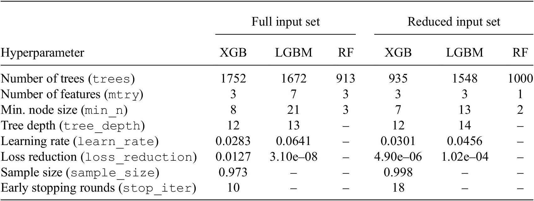
During model training, we employed repeated K-fold cross-validation combined with Bayesian optimization for hyperparameter tuning. K-fold cross-validation is a resampling method known to yield less biased performance estimates (Jung, Reference Jung2018); the dataset is randomly shuffled and split into K folds, with each fold serving once as the holdout while the model is trained on the remaining folds. Repeating this process R times further ensures robust estimates and helps prevent overfitting (Berrar, Reference Berrar2019). In our study, each model was trained using five folds repeated three times. For hyperparameter tuning, we utilized Bayesian optimization, which builds a probabilistic model of the objective function to iteratively select promising hyperparameter configurations, based on which hyperparameter settings are likely to reduce the loss according to patterns learned during the search, thereby efficiently exploring the hyperparameter space (Snoek et al., Reference Snoek, Larochelle and Adams2012). The final set of optimized hyperparameters is detailed in Table 3.
Final hyperparameter choices for models trained with full input set versus reduced input set
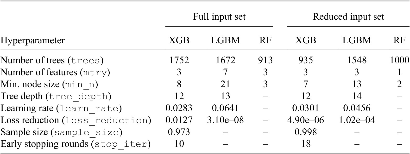
Table 3. Long description
The table is organized with hyperparameters in the first column, followed by two main categories: Full input set and Reduced input set. Each category contains columns for X G B, L G B M, and R F models.
* Number of trees (trees): Full set (X G B: 1752, L G B M: 1672, R F: 913); Reduced set (X G B: 935, L G B M: 1548, R F: 1000).
* Number of features (mtry): Full set (X G B: 3, L G B M: 7, R F: 3); Reduced set (X G B: 3, L G B M: 3, R F: 1).
* Min. node size (min sub n): Full set (X G B: 8, L G B M: 21, R F: 3); Reduced set (X G B: 7, L G B M: 13, R F: 2).
* Tree depth (tree underscore depth): Full set (X G B: 12, L G B M: 13, R F: not applicable); Reduced set (X G B: 12, L G B M: 14, R F: not applicable).
* Learning rate (learn underscore rate): Full set (X G B: 0.0283, L G B M: 0.0641, R F: not applicable); Reduced set (X G B: 0.0301, L G B M: 0.0456, R F: not applicable).
* Loss reduction (loss underscore reduction): Full set (X G B: 0.0127, L G B M: 3.10e-08, R F: not applicable); Reduced set (X G B: 4.90e-06, L G B M: 1.02e-04, R F: not applicable).
* Sample size (sample underscore size): Full set (X G B: 0.973, L G B M: not applicable, R F: not applicable); Reduced set (X G B: 0.998, L G B M: not applicable, R F: not applicable).
* Early stopping rounds (stop underscore iter): Full set (X G B: 10, L G B M: not applicable, R F: not applicable); Reduced set (X G B: 18, L G B M: not applicable, R F: not applicable).
Note. Hyperparameters were optimized using Bayesian optimization and cross-validation. Missing values indicate parameters that do not apply to those models.
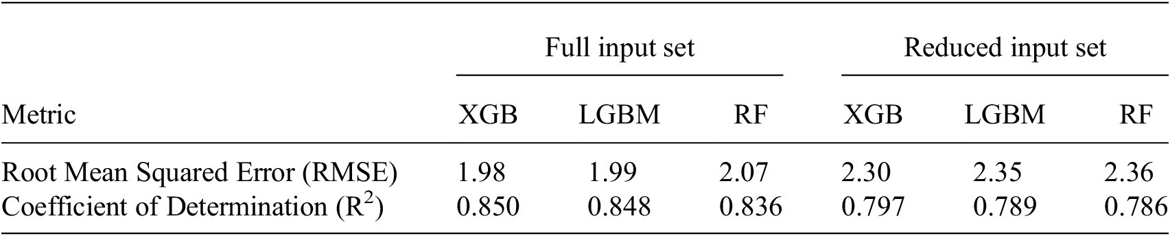
In evaluating our ML models, we relied on the coefficient of determination (
$ {R}^2 $
 ) and the root mean squared error (RMSE). RMSE quantifies the average magnitude of the errors between the predicted and actual values, meaning that a lower RMSE reflects a closer fit to the data. Conversely,
$ {R}^2 $
) and the root mean squared error (RMSE). RMSE quantifies the average magnitude of the errors between the predicted and actual values, meaning that a lower RMSE reflects a closer fit to the data. Conversely,
$ {R}^2 $
 indicates the proportion of variance in the target variable that the model can explain, with values near 1 denoting strong predictive power. The hyperparameters of our models were tuned with a focus on minimizing RMSE. The resulting metrics are presented in Table 4.
Model performance metrics for full input set versus reduced input set
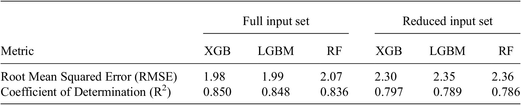
Table 4. Long description
The table is organized into seven columns. The first column lists the metrics, while the remaining six columns are grouped under two main headers: Full input set and Reduced input set. Each group contains three sub-columns for the models: X G B, L G B M, and R F.
Row 1: Root Mean Squared Error R M S E.
- Full input set: X G B is 1.98, L G B M is 1.99, R F is 2.07.
- Reduced input set: X G B is 2.30, L G B M is 2.35, R F is 2.36.
Row 2: Coefficient of Determination R super 2.
- Full input set: X G B is 0.850, L G B M is 0.848, R F is 0.836.
- Reduced input set: X G B is 0.797, L G B M is 0.789, R F is 0.786.
The data shows that the Full input set consistently yields lower R M S E and higher R super 2 values across all three models compared to the Reduced input set.
Note. Performance was evaluated using root mean squared error (RMSE) and the coefficient of determination (R2) on the test set. The comparison highlights the effect of using full input set versus reduced input set.
2.2.2. XGBoost model
XGBoost (eXtreme Gradient Boosting) builds a model using boosting, which adds many small decision trees one after another, where each new tree focuses on the errors the current model is still making, with the final prediction being the sum of all these trees (Chen and Guestrin, Reference Chen and Guestrin2016). XGBoost uses a small learning rate so each tree makes only a modest correction, limits tree depth to reduce overfitting, and adds penalties that discourage overly complex models. It also handles missing values automatically and trains quickly on large tabular datasets. These features make it a strong choice when relationships are non-linear and variables interact. In this study, we used the open-source xgboost library (v2.1.3; https://github.com/dmlc/xgboost, last access: November 2024).
2.2.3. LGBM model
Light Gradient Boosting Machine (LightGBM) is a method that combines many small decision trees to make predictions (Ke et al., Reference Ke, Meng, Finley, Wang, Chen, Ma, Ye and Liu2017). It is designed to work efficiently with large datasets and many predictor variables. To speed up training without losing accuracy, LightGBM gives more attention to the difficult cases that the model has trouble predicting and less to the easy ones. It also reduces the number of input columns by combining features that do not overlap in use. Together, these techniques allow the model to learn quickly while using less memory. These properties make LightGBM a good fit for data with interacting predictors and large sample sizes. In this study, we trained models with the LightGBM library (v4.5.0; https://github.com/Microsoft/LightGBM, last access: November 2024).
2.2.4. Random forest model
Random Forest (RF) builds many decision trees on different bootstrap samples of the training data and then averages their predictions (Breiman, Reference Breiman2001). At each split, a tree considers only a random subset of predictors, which makes the trees less similar to one another and helps prevent overfitting. Averaging many diverse trees reduces variance and usually gives strong, stable predictions across large tabular datasets (Fernández-Delgado et al., Reference Fernández-Delgado, Sirsat, Cernadas, Alawadi, Barro and Febrero-Bande2019; Cai et al., Reference Cai, Xu, Zhu, Hu and Li2020; Liu et al., Reference Liu, Zuo, Wang, Yuan, Zhu, Zhang, Zhang, Sun, Guo, Guo, Song, Song and Xu2021; Abbasian et al., Reference Abbasian, Solgi, Hosseini and Kia2022). Unlike boosting methods (e.g., XGBoost/LightGBM), RF grows trees independently and combines them at the end. In this study, we used the ranger library for RF regression (v0.13.1; https://github.com/imbs-hl/ranger, last access: November 2024).
2.3. Explanatory methods
To understand when and why our models change their NEE predictions, we use SHAP (SHapley Additive exPlanations) (Lundberg and Lee, Reference Lundberg and Lee2017; Molnar et al., Reference Molnar, Casalicchio and Bischl2018), a model-agnostic approach that decomposes each prediction into additive feature contributions for a given sample. For instance
$ x $
 , SHAP expresses the model output as
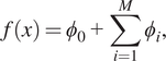
where
$ {\phi}_0=\unicode{x1D53C}\left[f(X)\right] $
 is the model’s baseline (average) prediction,
$ M $
is the model’s baseline (average) prediction,
$ M $
 is the number of features, and
$ {\phi}_i $
is the number of features, and
$ {\phi}_i $
 is the contribution of the feature
$ i $
is the contribution of the feature
$ i $
 for that sample. A positive
$ {\phi}_i $
for that sample. A positive
$ {\phi}_i $
 pushes the prediction up relative to the baseline; a negative
$ {\phi}_i $
pushes the prediction up relative to the baseline; a negative
$ {\phi}_i $
 pushes it down;
$ \mid {\phi}_i\mid $
pushes it down;
$ \mid {\phi}_i\mid $
 reflects the strength of influence in the same units as the model output, in our case, NEE
$ \mu $
reflects the strength of influence in the same units as the model output, in our case, NEE
$ \mu $
 mol s
$ {}^{-1} $
mol s
$ {}^{-1} $
 m
$ {}^{-2} $
m
$ {}^{-2} $
 .
.
SHAP satisfies useful properties for interpretation: local accuracy (additivity matches the model’s output for the sample), missingness (absent features have zero contribution), and consistency (if the model relies more on a feature, its attribution does not decrease) (Lundberg and Lee, Reference Lundberg and Lee2017). In practice, SHAP explanations help identify which predictors drive individual estimates and provide a global ranking aligned with model behavior. We note that SHAP explains the model’s reasoning rather than causality; correlated predictors can share credit, so related variables are interpreted together (Molnar et al., Reference Molnar, Casalicchio and Bischl2018).
We computed per-instance attributions with the TreeSHAP algorithm, which provides fast (polynomial-time) SHAP values for tree ensembles (Lundberg et al., Reference Lundberg, Erion, Chen, DeGrave, Prutkin, Nair, Katz, Himmelfarb, Bansal and Lee2019). We used the open-source treeshap package (v0.3.1; https://github.com/ModelOriented/treeshap, last access: November 2024). We applied SHAP only to held-out test observations to avoid bias from explaining training points and to reflect out-of-sample behavior. To summarize importance across the dataset, we report mean absolute SHAP per feature; where informative, we include SHAP dependence plots (feature value vs. SHAP contribution) to show directionality and reveal interactions.
3. Results and discussion
In this section, we discuss the results obtained with different models as well as different input variable configurations shown in Table 4. Unless otherwise stated, NEE denotes the eddy-covariance–measured flux; machine-learning–predicted NEE is not analyzed. First, in Section 3.1 we assess the models’ performance with accuracy metrics
$ {R}^2 $
 and RMSE, then visualize and analyze the SHAP values with a focus on the visualization and analysis of the SHAP values of DiffPAR.
In Section 3.2 we analyze the overall trends of the SHAP values across different input sets and ML models. In Sections 3.3 and 3.4, we present an in-depth SHAP analysis using the XGBoost model trained on a reduced input set (four variables), as well as discuss similar studies. Due to the high dimensionality of SHAP values, this simplified model was chosen to enhance interpretability while retaining strong predictive performance and ensuring the reliability of the insights.
3.1. Assessing model performance using accuracy metrics
Table 4 shows the root mean squared errors and coefficients of determination for all three different ML models and the two different input variable configurations. In general, the models performed better when trained on the full input set, as seen from the higher
$ {R}^2 $
 and lower RMSE. However, the
$ {R}^2 $
and lower RMSE. However, the
$ {R}^2 $
 is high, at almost 0.8, for reduced input set models as well. The difference between
$ {R}^2 $
is high, at almost 0.8, for reduced input set models as well. The difference between
$ {R}^2 $
 and RMSE for the different input set configurations is around
$ \simeq $
and RMSE for the different input set configurations is around
$ \simeq $
 0.05–0.06 and
$ \simeq $
0.05–0.06 and
$ \simeq $
 0.30–0.32, respectively. This difference is small enough to consider even the reduced input set models to model NEE well, but also high enough to indicate that the additional variables do contain information about NEE for slightly more accurate predictions.
For the reduced input set, all three models perform well, including RF, which is only slightly worse than the more advanced models XGBoost and LGBM. As RF is a slightly less complex model compared to XGBoost and LGBM, containing less tunable hyperparameters, this result is to be expected. For the full input set, RF is again the worst model, which is to be expected due to the previously stated reason; however, here the difference is noticeably larger, highlighting how the more complex models find more information from the full input set. Overall, it can be deduced that all models capture the relationship between NEE and the input variables well, and that these data are well suited for modeling NEE efficiently, even when using the reduced input set containing only four variables.
In a similar study, Abbasian et al. (Reference Abbasian, Solgi, Hosseini and Kia2022) used ML on flux-tower data to predict daily NEE in various European ecosystems. For evergreen needle-leaf forests, their models achieved
$ {R}^2 $
 values between 0.80 and 0.88. Our scores fall into the same range; however, we used slightly different input variables and instead modeled 30-min fluxes compared to daily fluxes. Another study by Liu et al. (Reference Liu, Zuo, Wang, Yuan, Zhu, Zhang, Zhang, Sun, Guo, Guo, Song, Song and Xu2021) showed similar ranges of
$ {R}^2 $
values between 0.80 and 0.88. Our scores fall into the same range; however, we used slightly different input variables and instead modeled 30-min fluxes compared to daily fluxes. Another study by Liu et al. (Reference Liu, Zuo, Wang, Yuan, Zhu, Zhang, Zhang, Sun, Guo, Guo, Song, Song and Xu2021) showed similar ranges of
$ {R}^2 $
 of 0.89–0.90 for modeling NEE using ML in evergreen needle-leaf forests for daily fluxes. An important notion is that the dataset in the present study is dominated by Hyytiälä data, as seen from Table 2, and according to our previous study (Ezhova et al. Reference Ezhova, Laanti, Lintunen, Kolari, Nieminen, Mammarella, Heljanko and Kulmala2025a), Hyytiälä was modeled better than Värriö. This suggests that Värriö and Järvselja may be more challenging for the ML models, possibly due to factors such as limited data or higher variability, which might explain the reduced overall performance.
3.2. SHAP summary: visualization of feature effects
We now consider SHAP values, allowing us to analyze how models see the relationship between input variables and the target variable, NEE. With baseline
$ {\phi}_0=-3.269194\mu \mathrm{mol}\hskip0.1em {\mathrm{m}}^{-2}\hskip0.1em {\mathrm{s}}^{-1} $
 , SHAP values measure how each feature shifts the prediction from this mean: negative values indicate stronger uptake (more negative NEE), while positive values indicate stronger respiration (more positive NEE).
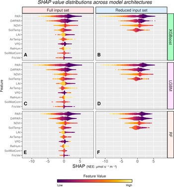
Here, we consider the SHAP values, using the beeswarm summary plot seen in Figure 1. This summary plot presents a compressed overview of how the input variables impact the model’s output. In order to make the plot easier to understand, all ordering is based on the results of the XGBoost model, the best-performing model.
Beeswarm summary plots of SHAP values showing the influence of input variables on NEE predictions across models and input configurations. PAR, DiffPAR, NDVI, and soil temperature consistently show the strongest effects. Despite variations in model type and input set, overall SHAP patterns remain similar, indicating robust relationships between input variables and NEE.
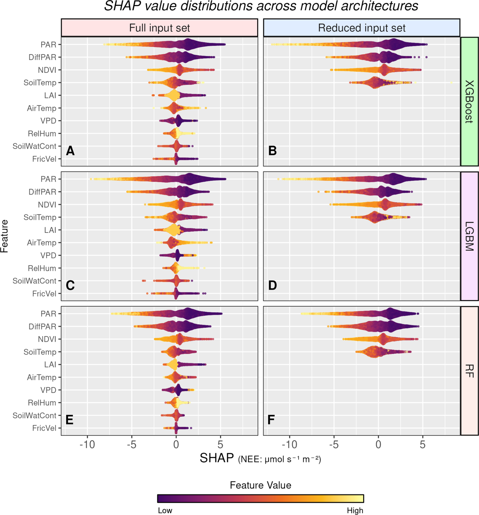
Figure 1. Long description
A grid of six beeswarm plots organized into three rows and two columns.
Axes and Legend:
* The vertical y-axis lists features: P A R, Diff P A R, N D V I, Soil Temp, L A I, Air Temp, V P D, Rel Hum, Soil Wat Cont, and Fric Vel.
* The horizontal x-axis represents the S H A P value for N E E in micromoles per second per square meter, ranging from negative 10 to positive 5.
* A color scale at the bottom indicates Feature Value, ranging from dark purple for Low to bright yellow for High.
Grid Layout:
* Left Column (Panels A, C, E): Full input set containing all ten features.
* Right Column (Panels B, D, F): Reduced input set containing only the top four features: P A R, Diff P A R, N D V I, and Soil Temp.
* Top Row (Panels A and B): X G Boost model.
* Middle Row (Panels C and D): L G B M model.
* Bottom Row (Panels E and F): R F model.
Data Trends:
* Across all panels, P A R and Diff P A R show the widest horizontal spread, indicating the strongest influence on N E E. High feature values (yellow) for these variables generally correlate with negative S H A P values.
* N D V I and Soil Temp show moderate spread, with high values typically associated with positive S H A P values.
* The distribution patterns for the top four features remain highly consistent regardless of whether the model uses the full or reduced input set or which of the three model architectures is employed.
For the full input set (Figures 1a, 1c, 1e), all ML models agree that the four variables that have the largest scale of effect on NEE are PAR, DiffPAR, NDVI, and soil temperature as indicated by the highest mean absolute SHAP values (global importance). These variables can be considered to be the ones with the most explanatory power, with PAR being the clear first in each case. This ranking is expected: these variables control light quantity and quality for photosynthesis, temperature-driven respiration, and canopy greenness. Because the study sites are temperature-limited and relatively humid, VPD and water availability contribute less at the annual scale (Ezhova et al., Reference Ezhova, Aarne, Arola, Lipponen, Lintunen, Kokkola, Ylivinkka, Yli-Juuti, Petäjä, Kerminen, Virtanen and Kulmala2025b).
PAR is theoretically the most important variable to explain photosynthesis, especially during the peak growing season (Palmroth and Hari, Reference Palmroth and Hari2001; Moffat et al., Reference Moffat, Beckstein, Churkina, Mund and Heimann2010). These results are consistent with previous results (Ezhova et al., Reference Ezhova, Laanti, Lintunen, Kolari, Nieminen, Mammarella, Heljanko and Kulmala2025a) from the same forest sites, where PAR, DiffPAR, and SoilTemp were the main drivers. The effect of DiffPAR on photosynthesis is also well known (Gu et al., Reference Gu, Baldocchi, Verma, Black, Vesala, Falge and Dowty2002), with canopies with higher LAI benefiting more from diffuse radiation (Durand et al., Reference Durand, Murchie, Lindfors, Urban, Aphalo and Robson2021).
While the light-related variables are considered to be the most important to explain NEE, the third variable in importance is NDVI, most likely important due to it being a good proxy for the fraction of absorbed PAR (Balzarolo et al., Reference Balzarolo, Vicca, Nguy-Robertson, Bonal, Elbers, Fu, Grünwald, Horemans, Papale, Peñuelas, Suyker and Veroustraete2016), and reflecting seasonality and the average age of the leaves. NDVI is also distinct enough in the different sites to act as a possible site-identifier proxy. Soil temperature, on the other hand, can model respiration, as respiration is highly sensitive to temperature, while also capturing seasonality. While the model clearly uses air temperature to some degree as well, it has been noted in some previous studies that soil temperature may be a better parameter than air temperature for modeling ecosystem respiration (Kolari et al., Reference Kolari, Kulmala, Pumpanen, Launiainen, Ilvesniemi, Hari and Nikinmaa2009; Lasslop et al., Reference Lasslop, Migliavacca, Bohrer, Reichstein, Bahn, Ibrom, Jacobs, Kolari, Papale, Vesala, Wohlfahrt and Cescatti2012). Several of the remaining input variables are highly correlated with the four most important ones—for example, soil temperature is closely related to air temperature—which may cause the model to either prioritize one or split the explanatory power between them (Moffat et al., Reference Moffat, Beckstein, Churkina, Mund and Heimann2010). However, they still contribute to the model, and since SHAP can split contributions among correlated inputs (Molnar, Reference Molnar2025), the importance of these variables may be divided.
When considering the contributions of the individual feature values, the SHAP values demonstrate that they capture these contributions consistently, regardless of the model or input configuration used. The plots show that higher radiation drives more negative NEE (higher carbon uptake), while lower radiation produces higher NEE. This pattern aligns with both diurnal and seasonal cycles, so that the highest-radiation points (midday in peak growing season) contribute most strongly to NEE. NDVI behaves differently from radiation variables because it does not change over the course of a single day but instead reflects seasonality. Instead, NDVI’s influence is subtler: data points associated with more negative NEE (greater uptake) tend to have slightly higher NDVI than those linked to positive NEE, even though NDVI remains essentially constant between morning, midday, and evening. The fourth parameter is soil temperature, for which SHAP clearly shows that the dependence is nonlinear, as we see points with high soil temperature on both sides of the SHAP values. Leaf area index (LAI) is the variable that differs most across the sites, where low LAI values correspond exclusively to Värriö, which also has the lowest overall NEE from the studied sites due to it being in a much northern region, making it most likely the variable the models use to identify the site, similarly to NDVI. VPD, relative air humidity, soil water content, and friction velocity all contribute to the predictions on a small scale, and as previously mentioned, they are highly dependent on other variables, leading to them having a smaller scale of impact.
All three different ML models exhibit similar overall patterns in SHAP values, but LGBM shows more distinctive behavior, while XGBoost and random forest are more alike. The shapes and the colors of the distributions of the SHAP values are similar; however, the scales vary. PAR has a larger scale in LGBM (Figure 1c), providing SHAP values up to −9, while random forest and XGBoost have only values up to around −7.5 (Figure 1a, e). Reducing the input variables makes the scales of the four variable larger, as is expected due to the need to compensate for the effect of the removed variables, making the PAR SHAP values as high as −12 in LGBM and XGBoost (Figure 1b, d). It would seem that when using the reduced variable set, the positive effects of any features omitted from that set are absorbed by PAR and NDVI, while the negative effects are captured by soil temperature (Figure 1b, d, f). However, the distributions remain similar in shape and color, suggesting that they are still modeled largely in the same way, whether additional variables are included, suggesting a robust relationship between the main input variables and NEE. Due to the large dimensionality of the SHAP values, only general trends can be observed from Figure 1, highlighting the need for a different kind of visualization to observe more detailed relationships, provided in the next section.
3.3. Dependence of NEE on different variables visualized with SHAP values
In this section, we consider SHAP values based on individual features and plot them using scatter plots and box plots to analyze the interactions between different variables. While previous studies exist that use SHAP values to analyze ML models of NEE (Gao et al., Reference Gao, Yao, Gao, Yuan, He, Wang, Li, Ma, Russell, Pressley and Zou2024; Chen et al., Reference Chen, Wu, Chen and Wan2025), they mostly focus on an overview of the variable effects using plots similar to those seen in Figure 1. While this type of figure effectively captures the general relationship between input variables and the target variable through SHAP values, it does not reveal how features interact with one another or the underlying nature of these dependencies.
We can analyze the impact of variables of interest on NEE in more detail. All SHAP values in this and the following section come from the XGBoost model trained on the reduced input variable set (PAR, DiffPAR, NDVI, and Soil Temperature). To reveal how variables interact, the scatter plots are colored according to another selected variable. This approach highlights how the SHAP values of one predictor change in relation to variations in another, making the dependencies between drivers more visible.
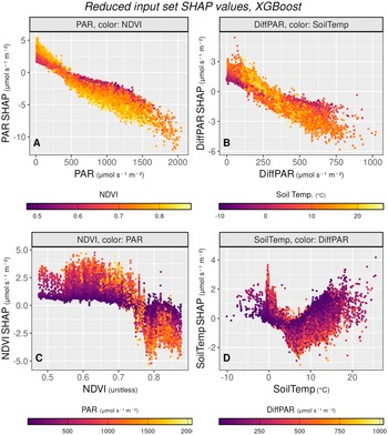
Figure 2 shows the PAR, DiffPAR, NDVI, and SoilTemp on the X axis with the corresponding SHAP values on the Y axis. The coloring of the plots was chosen based on which variable interactions we wanted to observe in more detail. Figure 2a, featuring PAR and PAR SHAP, shows the slightly nonlinear interaction between PAR and NEE. As PAR increases, so does its contribution toward more negative NEE. This is consistent with increasing radiation contributing toward more photosynthesis (and thus reduced NEE) as mentioned in the previous subsection. NDVI was chosen as the coloring to demonstrate how seasonality interacts with PAR. A low NDVI, corresponding to points in winter, early spring, or late autumn, restricts the effect of PAR, as lower leaf biomass means less absorption of radiation and less photosynthesis, but also less respiration. Conversely, high NDVI values correspond to the highest range of SHAP change across PAR levels, meaning that the highest increase in carbon uptake due to PAR is reached when the NDVI is high, but also the highest emissions of carbon under low PAR occur when the NDVI is high. The PAR SHAP values have the highest absolute effect range on NEE, reflecting the perceived importance of the variable.
Figure 2b visualizes DiffPAR and DiffPAR SHAP. It demonstrates that as DiffPAR increases, so does the carbon sink. Here we can also see how soil temperature interacts with the effect of DiffPAR on NEE: lower soil temperature is linked to more negative NEE when DiffPAR is low, around <200
$ \mu \mathrm{mol}\;{\mathrm{m}}^{-2}\;{\mathrm{s}}^{-1} $
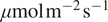 , while higher soil temperature is linked to more negative NEE when DiffPAR is high, around >300
$ \mu \mathrm{mol}\;{\mathrm{m}}^{-2}\;{\mathrm{s}}^{-1} $
, while higher soil temperature is linked to more negative NEE when DiffPAR is high, around >300
$ \mu \mathrm{mol}\;{\mathrm{m}}^{-2}\;{\mathrm{s}}^{-1} $
 . This interaction reflects seasonal patterns, where DiffPAR has little effect on NEE under cold soil conditions, likely due to limited photosynthetic activity (Lintunen et al., Reference Lintunen, Paljakka, Salmon, Dewar, Riikonen and Hölttä2020). The strongest contribution of DiffPAR to carbon uptake appears under moderate soil temperatures, typically in late spring or early summer, while its effect diminishes again at the highest temperatures.
SHAP dependence plots for the reduced input XGBoost model, showing how PAR, DiffPAR, NDVI, and soil temperature influence NEE predictions. Each subfigure plots a variable against its SHAP value, with color indicating a second interacting variable. The plots reveal seasonal and interaction effects, such as stronger PAR and DiffPAR contributions to carbon uptake under high NDVI or moderate soil temperatures, and that soil temperature acts more as a modulating factor than a primary driver.
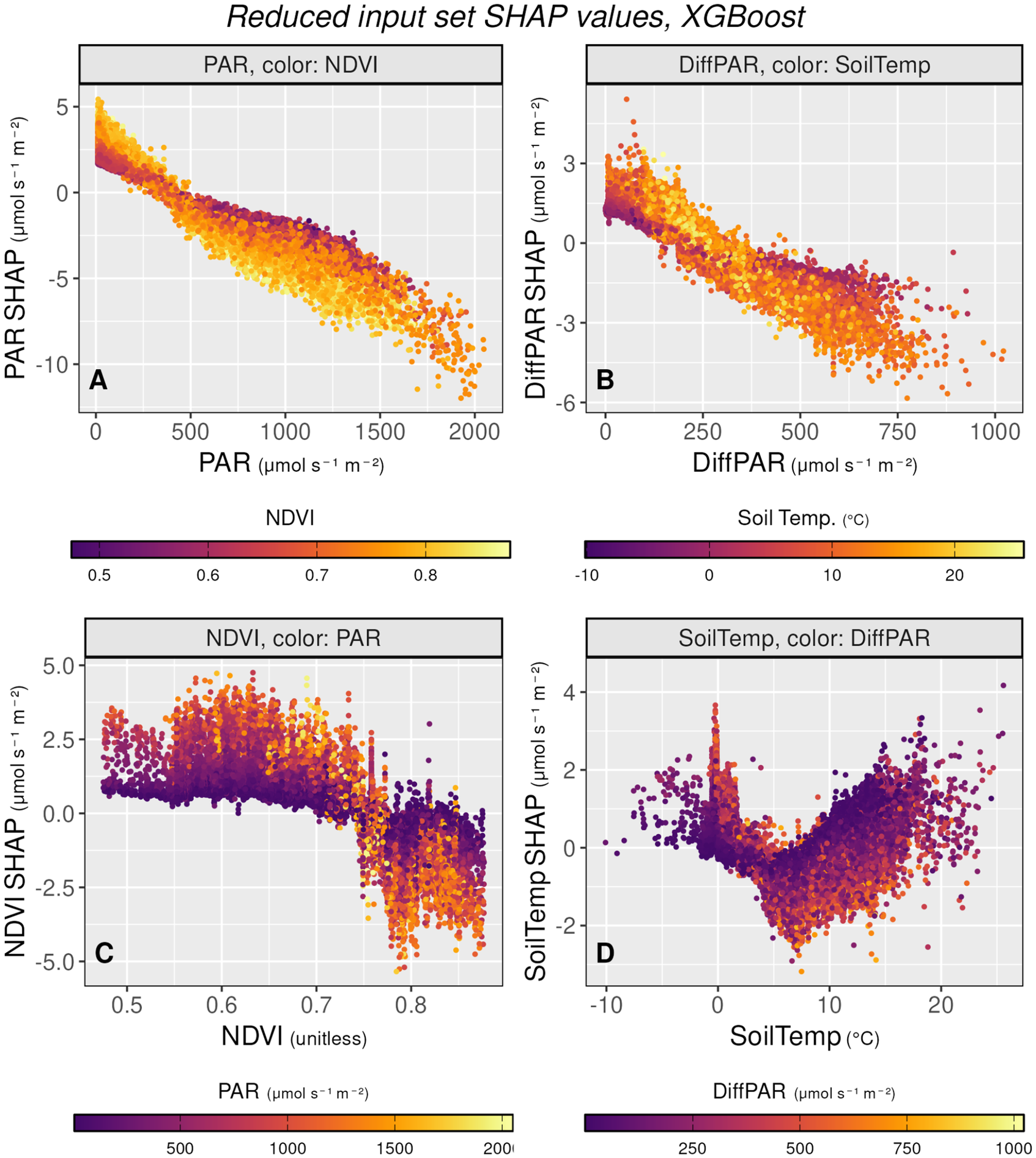
Figure 2. Long description
Four scatter plots arranged in a two-by-two grid. All y-axes represent S H A P values in micromoles per second per meter squared.
Panel A, top-left. X-axis is P A R from 0 to 2000 micromoles per second per square meter. The data shows a strong negative linear trend where S H A P values decrease from positive 5 to negative 10 micromoles per second per meter squared as P A R increases. Points are color-coded by N D V I from 0.5 purple to 0.8 yellow, showing higher N D V I values correlate with more negative S H A P values at high P A R.
Panel B, top-right. X-axis is Diff P A R from 0 to 1000 micromoles per second per square meter. A negative trend is visible, with S H A P values dropping from 3 to negative 6 micromoles per second per square meter. Points are color-coded by Soil Temp from negative 10 degrees Celsius purple to 20 degrees Celsius yellow.
Panel C, bottom-left. X-axis is N D V I unitless from 0.5 to 0.8. The data remains relatively flat near a S H A P value of 2 micromoles per second per square meter until N D V I reaches 0.75, where it drops sharply toward negative 5 micromoles per second per square meter. Points are color-coded by P A R from 500 purple to 2000 yellow, in units of micromoles per second per square meter.
Panel D, bottom-right. X-axis is Soil Temp from negative 10 to 20 degrees Celsius. The data forms a V-shape with a trough near 8 degrees Celsius where S H A P values reach negative 2, then rise back toward positive 4 micromoles per second per square meter at higher temperatures. Points are color-coded by Diff P A R from 250 purple to 1000 yellow, in units of micromoles per second per square meter.
In Figure 2c NDVI’s SHAP is shown against NDVI with PAR coloring. This plot integrates the effect of station and seasonality on NEE. The high NDVI region corresponds to the peak growing season at the southern stations, when high radiation greatly increases photosynthesis, whereas during autumn/spring, high PAR corresponds to high carbon emissions. As high NDVI corresponds to plants being able to absorb radiation (Balzarolo et al., Reference Balzarolo, Vicca, Nguy-Robertson, Bonal, Elbers, Fu, Grünwald, Horemans, Papale, Peñuelas, Suyker and Veroustraete2016), this is also a logical conclusion from the models. Lower NDVI values are also more common in Värriö, which has systematically more positive NEE, which might also help to explain why lower NDVI values have higher SHAP values.
Finally, Figure 2d shows soil temperature and its SHAP values. Among the four input variables in the reduced input set, soil temperature has the lowest impact, suggesting that the ML models treat it more as a supporting factor rather than a direct driver of NEE. The seasonal pattern is visible here: as soil temperature rises to around 7°C, the carbon sink increases. However, at higher temperatures, the effect reverses, and further increases in soil temperature lead to positive SHAP contributions for NEE, likely due to stronger temperature-dependent respiration that pushes NEE toward higher values. The color shading represents diffuse PAR levels, showing that diffuse PAR has a positive effect on the carbon sink at higher soil temperatures, but a negative effect when the soil is cold.
While these plots are insightful and help validate that the models behave intuitively and reproduce the expected ecology, they do not contain much new information. To gain more insight from SHAP values, we next employ plots with a different approach.
3.4. DiffPAR SHAP values
Diffuse radiation was chosen as an input variable of interest for more detailed analysis due to open questions about the effects of diffuse radiation on forest carbon sinks, such as whether it is more mediated through clouds or aerosol (van Diepen et al., Reference van Diepen, Kaiser, Hartogensis, Graf, de Arellano and Moene2025).
SHAP values can reveal context-dependent interactions between diffuse radiation, NEE, and other variables. This motivates moving from SHAP as a model validation step to using SHAP to stratify the data. Here we use DiffPAR SHAP values to form groups and compare them with simple DiffPAR thresholding; the results suggest a clearer diffuse-light (cloud-related) enhancement of carbon uptake, motivating our climate-relevant discussion of how cloudiness and aerosol-driven scattering may influence NEE.
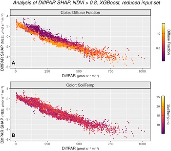
Figures 3 and 4 summarize how the model attributes diffuse radiation effects and how this relates to observed NEE. Figure 3 plots DiffPAR against its SHAP values with points colored by co-variates, using only observations with NDVI >0.8 to reduce the influence of seasonal variation. In Figure 3a (colored by diffuse fraction, a variable not included in the model), within intermediate DiffPAR (approximately 100–500
$ \mu \mathrm{mol},{\mathrm{m}}^{-2},{\mathrm{s}}^{-1} $
 ), SHAP contributions become increasingly negative as diffuse fraction increases, consistent with a stronger carbon sink under high diffuse fraction indicating overcast skies. This can be due to differences in the spectral distribution of diffuse radiation between rather clear and overcast skies, that is, the distribution of incoming radiation across wavelengths can differ between these two cases. Moreover, Figure 3a shows a distinct pattern around DiffPAR SHAP
$ \approx -2 $
), SHAP contributions become increasingly negative as diffuse fraction increases, consistent with a stronger carbon sink under high diffuse fraction indicating overcast skies. This can be due to differences in the spectral distribution of diffuse radiation between rather clear and overcast skies, that is, the distribution of incoming radiation across wavelengths can differ between these two cases. Moreover, Figure 3a shows a distinct pattern around DiffPAR SHAP
$ \approx -2 $
 : when DiffPAR SHAP values are
$ \ge -2 $
: when DiffPAR SHAP values are
$ \ge -2 $
 , the separation between overcast and clear-sky cases becomes especially clear, whereas values
$ <-2 $
, the separation between overcast and clear-sky cases becomes especially clear, whereas values
$ <-2 $
 are associated with patchy cloud conditions. Diffuse radiation is particularly enhanced under patchy clouds, which are known to exert the strongest positive effect on photosynthesis. For this reason, we selected
$ -2 $
are associated with patchy cloud conditions. Diffuse radiation is particularly enhanced under patchy clouds, which are known to exert the strongest positive effect on photosynthesis. For this reason, we selected
$ -2 $
 as the threshold in Figure 4, where we contrast high- and low-diffuse-radiation cases.
Alternative view of the DiffPAR–SHAP relationship (as in subfigure 2b), restricted to observations with NDVI
$ >0.8 $
 to reduce the influence of seasonal variation, and colored by diffuse fraction (3a) and soil temperature (3b). Subfigure 3a confirms that points with high DiffPAR and low PAR correspond to overcast conditions (high diffuse fraction). Subfigure 3b shows no clear pattern with soil temperature, indicating that the observed diffuse radiation effect on NEE is not driven by temperature.
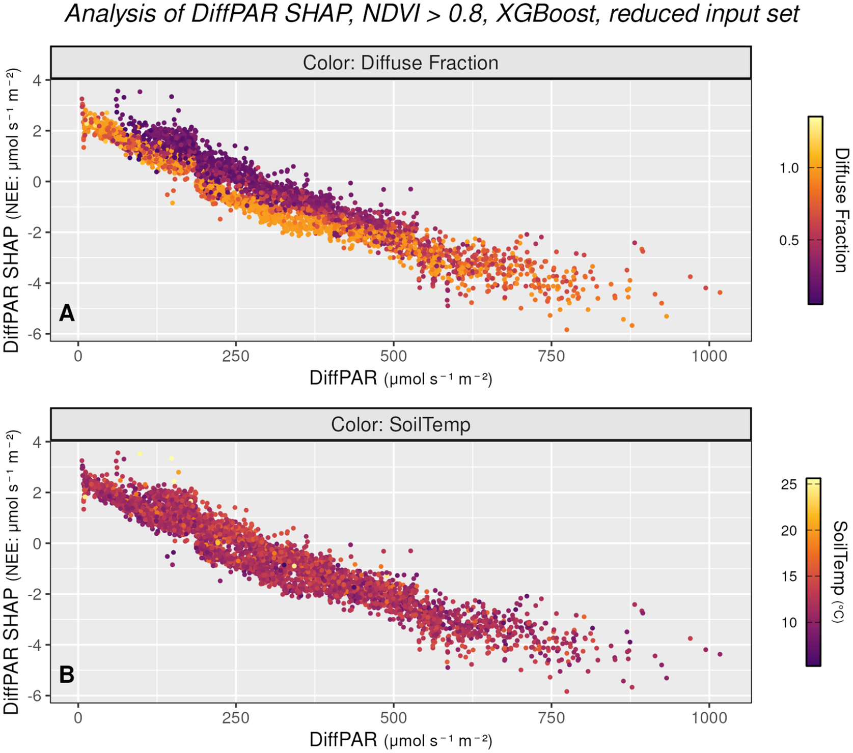
Figure 3. Long description
The figure consists of two vertically stacked scatter plots, labeled A and B, both sharing the same axes. The x-axis represents Diff P A R in micromoles per second per square meter, ranging from 0 to 1000. The y-axis represents Diff P A R S H A P for N E E in micromoles per second per square meter, ranging from negative 6 to 4 micromoles per second per square meter. Both plots show a strong negative linear correlation where S H A P values decrease as Diff P A R increases.
* Panel A is titled Color Diffuse Fraction. The data points are colored based on a gradient from dark purple (0.0) to bright yellow (1.0). Points with low Diff P A R (0 to 250 micromoles per second per square meter) and high S H A P values (0 to 4 micromoles per second per square meter) are predominantly yellow, indicating a high diffuse fraction. As Diff P A R increases, the points transition to orange and then purple.
* Panel B is titled Color Soil Temp. The data points are colored based on a gradient from dark purple (10 degrees Celsius) to bright yellow (25 degrees Celsius). Unlike panel A, the colors in panel B are mixed throughout the data cloud, showing no distinct spatial pattern or correlation between soil temperature and the Diff P A R S H A P relationship.
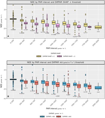
Comparison of reduced input XGBoost interpretation (4a) versus traditional data grouping (4b) for assessing the effect of DiffPAR. In 4a, data points with DiffPAR SHAP below −2 show lower NEE, supporting the model’s attribution of enhanced carbon uptake to diffuse radiation. In contrast, 4b shows a weaker relationship when NEE is grouped solely by raw DiffPAR thresholds, highlighting how SHAP reveals interaction-driven effects not apparent in direct data plots.
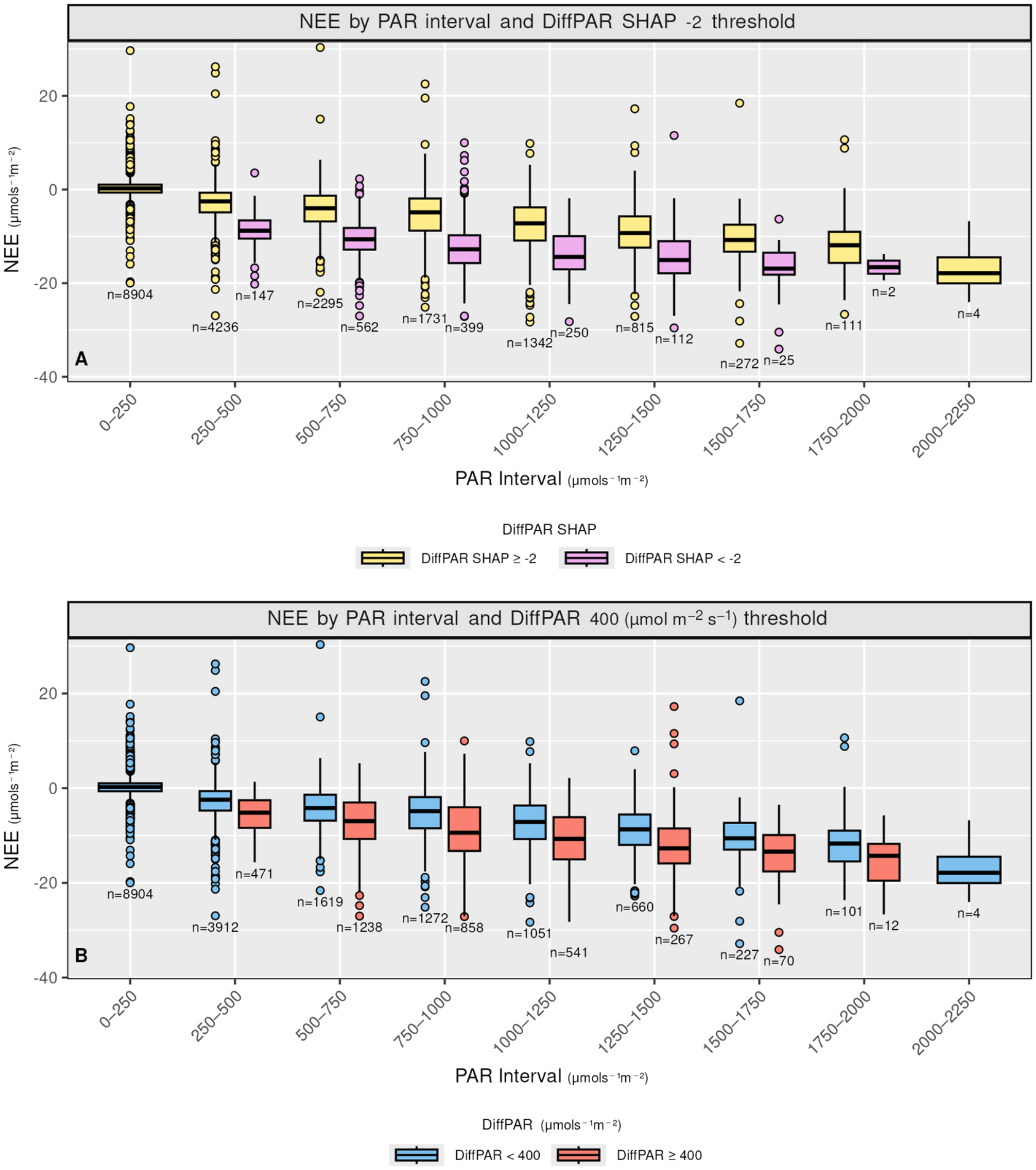
Figure 4. Long description
Two vertically stacked boxplot graphs labeled A and B. Both share a Y-axis of N E E in micromoles per second per square meter, ranging from negative 40 to 20, and an X-axis of P A R Interval in micromoles per second per square meter, divided into nine bins from 0 to 2250.
Panel A is titled N E E by P A R interval and Diff P A R S H A P negative 2 micromoles per second per square meter threshold. It compares two groups: Diff P A R S H A P greater than or equal to negative 2 micromoles per second per square meter in yellow and Diff P A R S H A P less than negative 2 micromoles per second per square meter in purple. As P A R increases, the purple boxes consistently show lower median N E E values compared to the yellow boxes, particularly in the 500 to 1500 micromoles per second per square meter range. Sample sizes n are noted below each box.
Panel B is titled N E E by P A R interval and Diff P A R 400 micromoles per second per square meter threshold. It compares Diff P A R less than 400 micromoles per second per square meter in blue and Diff P A R greater than or equal to 400 micromoles per second per square meter in red. The separation between the blue and red boxes is less pronounced than the separation in Panel A, with significant overlap in the interquartile ranges across most P A R intervals.
Both panels show a general trend of decreasing N E E as P A R increases, with outliers represented by individual circles above and below the whiskers.
In Figure 3b (colored by soil temperature), no comparable gradient is evident, indicating that the diffuse-radiation signal is not a proxy for thermal conditions and is unlikely to be explained by collinearity with temperature. These patterns pool observations across all sites, reinforcing the spatial robustness of the effect.
Figure 4 contrasts the DiffPAR SHAP grouping of
$ -2 $
 with raw DiffPAR grouping of 400
$ \mu \mathrm{mol},{\mathrm{m}}^{-2},{\mathrm{s}}^{-1} $
with raw DiffPAR grouping of 400
$ \mu \mathrm{mol},{\mathrm{m}}^{-2},{\mathrm{s}}^{-1} $
 , clarifying how diffuse radiation influences NEE through interactions rather than as a simple monotonic response. Importantly, both the SHAP-based and raw DiffPAR-based groupings contain a similar number of observations (i.e., roughly balanced
$ n $
, clarifying how diffuse radiation influences NEE through interactions rather than as a simple monotonic response. Importantly, both the SHAP-based and raw DiffPAR-based groupings contain a similar number of observations (i.e., roughly balanced
$ n $
 ), so the sharper separation in 4A, is not an artifact of uneven sample sizes. When defining the raw DiffPAR grouping, we selected a threshold of 400
$ \mu \mathrm{mol},{\mathrm{m}}^{-2},{\mathrm{s}}^{-1} $
), so the sharper separation in 4A, is not an artifact of uneven sample sizes. When defining the raw DiffPAR grouping, we selected a threshold of 400
$ \mu \mathrm{mol},{\mathrm{m}}^{-2},{\mathrm{s}}^{-1} $
 . This choice was motivated by Supplementary Figure A4C, where DiffPAR values separated by the
$ \mathrm{DiffPAR}\ \mathrm{SHAP}<-2 $
. This choice was motivated by Supplementary Figure A4C, where DiffPAR values separated by the
$ \mathrm{DiffPAR}\ \mathrm{SHAP}<-2 $
 threshold show division where, in the
$ \mathrm{DiffPAR}\ \mathrm{SHAP}<-2 $
threshold show division where, in the
$ \mathrm{DiffPAR}\ \mathrm{SHAP}<-2 $
 group, 400 lies below the lower quartile, while in the
$ \mathrm{DiffPAR}\ \mathrm{SHAP}\ge -2 $
group, 400 lies below the lower quartile, while in the
$ \mathrm{DiffPAR}\ \mathrm{SHAP}\ge -2 $
 group it lies above the upper quartile. This makes it a fitting boundary between conditions dominated by strong diffuse-radiation effects and those without. Moreover, a comparable threshold of approximately 200 W, m
$ {}^{-2} $
group it lies above the upper quartile. This makes it a fitting boundary between conditions dominated by strong diffuse-radiation effects and those without. Moreover, a comparable threshold of approximately 200 W, m
$ {}^{-2} $
 of diffuse radiation (equivalent to roughly 400
$ \mu \mathrm{mol},{\mathrm{m}}^{-2},{\mathrm{s}}^{-1} $
of diffuse radiation (equivalent to roughly 400
$ \mu \mathrm{mol},{\mathrm{m}}^{-2},{\mathrm{s}}^{-1} $
 PAR) was identified in our recent related work (Ezhova et al., Reference Ezhova, Aarne, Arola, Lipponen, Lintunen, Kokkola, Ylivinkka, Yli-Juuti, Petäjä, Kerminen, Virtanen and Kulmala2025b) as the point where diffuse radiation begins to have a beneficial effect on photosynthesis.
In Figure 4a, observations with
$ \mathrm{DiffPAR}\ \mathrm{SHAP}<-2 $
 , that is, cases where the model attributes a strong diffuse-radiation contribution, exhibit markedly lower (more negative) NEE on average; these points also have high DiffPAR (mean
$ =571.75\mu \mathrm{mol},{\mathrm{m}}^{-2},{\mathrm{s}}^{-1} $
, that is, cases where the model attributes a strong diffuse-radiation contribution, exhibit markedly lower (more negative) NEE on average; these points also have high DiffPAR (mean
$ =571.75\mu \mathrm{mol},{\mathrm{m}}^{-2},{\mathrm{s}}^{-1} $
 ), consistent with an enhanced carbon sink under diffuse-light conditions. By comparison, Figure 4b groups observations by raw DiffPAR thresholds alone and shows a much weaker separation in NEE, indicating that total DiffPAR without context is insufficient to isolate the effect. The stronger contrast in 4A implies that the model is able to disentangle the diffuse radiation effect from other variables; therefore, the model suggests that the diffuse radiation effect is larger compared to standard threshold-based analysis.
Overall, after excluding the lowest and highest PAR bins (0–250 and 2000–2250), the SHAP-stratified subset (
$ \mathrm{DiffPAR}\ \mathrm{SHAP}<-2 $
 ) has a median NEE that is
$ 1.545\mu \mathrm{mol},{\mathrm{m}}^{-2},{\mathrm{s}}^{-1} $
) has a median NEE that is
$ 1.545\mu \mathrm{mol},{\mathrm{m}}^{-2},{\mathrm{s}}^{-1} $
 more negative than the subset defined by raw
$ \mathrm{DiffPAR}\ge 400 $
more negative than the subset defined by raw
$ \mathrm{DiffPAR}\ge 400 $
 , indicating that the model-attributed signal isolates a stronger diffuse-light enhancement than raw DiffPAR alone.
Neimane-Šroma et al. (Reference Neimane-Šroma, Durand, Lintunen, Aalto and Robson2024) recently studied the diffuse radiation fertilization effect in a boreal Scots pine forest (SMEAR II forest) at ecosystem, branch, and ground vegetation scales, demonstrating that at equivalent total PAR, diffuse radiation conditions yield higher ecosystem productivity by enhancing photosynthesis across scales more than direct radiation conditions. Our SHAP-based analysis is novel in independently identifying this diffuse radiation fertilization as a distinct pattern in the model’s predictions, pointing to a previously unreported phenomenon from a modeling perspective. This explainable ML approach, therefore, complements and extends the physiological insights of Neimane-Šroma et al. (Reference Neimane-Šroma, Durand, Lintunen, Aalto and Robson2024), bridging their multi-scale gas-exchange findings with ecosystem-scale model behavior.
A plausible explanation is that under overcast (highly diffuse) skies, light penetrates deeper into the canopy and alleviates direct-radiation stress on sun-exposed foliage, giving the forest a net photosynthetic boost not offset by lower total PAR.
Since SHAP reveals the model’s internal logic rather than proving causality, targeted branch- and forest floor-level gas-exchange measurements during high-diffuse, low-PAR periods (as in Neimane-Šroma et al., Reference Neimane-Šroma, Durand, Lintunen, Aalto and Robson2024) are needed to verify the mechanism. If confirmed, this result implies that projected increases in cloudiness or aerosol-driven light scattering could make boreal forests stronger short-term CO2 sinks than current models assume, challenging the classical assumption that reduced PAR necessarily limits carbon uptake.
4. Conclusions
We used ML to model NEE at three different sites: one boreal forest site in southern Finland and one in the Finnish subarctic, as well as one hemiboreal forest site in Estonia. We focused on analyzing the ML models and confirming the conclusions of the models by comparing the results across two different sets of input variables and different types of ML models. NEE for multiple sites can be modeled reasonably well with only four variables reaching
$ {R}^2 $
 of
$ \approx 0.79 $
of
$ \approx 0.79 $
 and RMSE of
$ \approx 2.30 $
and RMSE of
$ \approx 2.30 $
 , while using more variables does make the models slightly more accurate, reaching
$ {R}^2\approx 0.85 $
, while using more variables does make the models slightly more accurate, reaching
$ {R}^2\approx 0.85 $
 and RMSE of
$ \approx 1.99 $
and RMSE of
$ \approx 1.99 $
 . However, four-variable models are much easier for analyzing the relationships between the input variables and NEE. The best-performing model was XGBoost, slightly outperforming LGBM and RF, with RF being slightly worse than XGBoost and LGBM.
The best variables to predict NEE are radiative variables PAR and DiffPAR across all models and input variable sets, followed by NDVI and soil temperature. Input variables air temperature, LAI, VPD, RH, soil water content, and friction velocity are all used by the models to make more accurate predictions, but improve the model accuracy only slightly, around
$ \approx $
 0.05 in R
$ {}^2 $
0.05 in R
$ {}^2 $
 score.
We also used SHAP values to analyze the relationships between the input variables and NEE. While previous studies have applied SHAP to NEE prediction (Gao et al., Reference Gao, Yao, Gao, Yuan, He, Wang, Li, Ma, Russell, Pressley and Zou2024; Chen et al., Reference Chen, Wu, Chen and Wan2025), they have typically done so in a limited or superficial way. Our SHAP results suggest that the models capture the relationships between input variables and NEE in line with current scientific understanding, meaning they reproduce expected dependencies under different environmental conditions. The overall variance in SHAP values was consistent across models with different input variable sets. As expected, SHAP contributions were more spread out when all input variables were included and more concentrated when using the reduced set of four variables. However, the overall patterns and shapes of the variable interactions remained largely unchanged regardless of the number of input variables used.
The SHAP results also revealed an interesting interaction between NEE and DiffPAR that the models picked up, where high PAR and low diffuse fraction correspond to clear sky conditions, and low PAR and high diffuse fraction to overcast skies. We found that overcast sky conditions have more negative DiffPAR SHAP than clear sky conditions, enhancing the carbon sink. This SHAP analysis suggests that the DiffPAR-induced decrease in NEE compensates for the increase in NEE due to low total radiation under an overcast sky. This effect is robust and consistent, as further SHAP analysis suggests that this effect is not due to the temperature but cloud-related phenomena. We also observe that high DiffPAR levels, which lead to low (i.e., strongly negative) DiffPAR SHAP values, are associated with low NEE values, indicating increased carbon uptake.
Importantly, SHAP values explain how the trained models use the available predictors to make predictions, rather than proving a causal mechanism. Because diffuse radiation co-varies with cloudiness and other meteorological factors, and because some relevant variables may be unobserved, we interpret the diffuse-radiation signal identified here as hypothesis-generating and as guidance for where targeted measurements and process-based analyses should focus. In this sense, the analysis does not directly explain causal effects, but instead provides one way to quantify the relative role of individual variables in a system shaped by many interacting drivers. The resulting interpretation should, therefore, not be seen as ground truth, but rather as a hypothesis based on what the model has learned from the data.
To summarize, ML models combined with XAI methods such as SHAP values can uncover previously unseen scientifically meaningful interactions between the studied variables. Yet SHAP values are inherently high-dimensional: every feature has its own SHAP value for every data point, and making sense of them requires strong domain knowledge. In practice, XAI methods are most powerful when paired with expert-guided visual exploration that is verified across multiple different variations of the data and also across different models. Otherwise, the high dimensionality of SHAP value risks making them becoming a relatively shallow look at the data, but with expert knowledge, they are a flexible way of analyzing and validating data.
Overall, this work contributes by demonstrating a robust explainable-ML workflow for ecosystem process analysis and by suggesting, across sites, that diffuse-radiation–related NEE responses emerge most clearly under interaction-defined regimes identified by the model.
Open peer review
To view the open peer review materials for this article, please visit http://doi.org/10.1017/eds.2026.10040.
Supplementary material
The supplementary material for this article can be found at http://doi.org/10.1017/eds.2026.10040.
Data availability statement
Replication data and code can be found in the Zenodo repository: https://doi.org/10.5281/zenodo.17396659.
Acknowledgments
The authors wish to acknowledge CSC – IT Center for Science, Finland, for computational resources. During the writing of the manuscript, the authors used ChatGPT by OpenAI (primarily GPT-4o, accessed between November 2024 and May 2025, chatgpt.com) to assist with grammar, wording, and clarity of the manuscript, as well as with drafting code used for training the models. The AI tool was not used to interpret the results, formulate the scientific arguments, generate new scientific content, create figures, or identify or generate references. The authors take full responsibility for the accuracy, integrity, and final content of the manuscript.
Author contribution
Conceptualization: T.L., E.E., K.H., and A.L.; Data curation: V.M., D.K., and S.M.N.; Formal analysis: T.L., E.E., K.H., and A.L.; Funding acquisition: M.K., A.L., and K.H.; Investigation: T.L. and A.A.; Methodology: T.L., E.E., K.H., and A.L.; Visualization: T.L.; Writing – original draft: T.L.; Writing – review and editing: T.L., A.A., A.L., M.D., K.H., S.M.N., V.M., D.K., M.K., and E.E. All authors approved the final submitted draft.
Ethics statement
The research meets all ethical guidelines, including adherence to the legal requirements of the study country.
Funding statement
This research was supported by the Academy of Finland (ACCC Flagship, grant 337,549; projects 347,780 and 347,782 “ForClimate”; Academy Research Fellow project 355,142; ACCC continuation 359,340), the Research Council of Norway (grants 322,317 and 351,754), and the Estonian Research Council (grant PRG1674). We also acknowledge support from the CarbonSink+ of Forests project (Ministry-funded).
Competing interests
None.




 Open access


Comments
Dear Editor,
Please find attached the manuscript entitled «Explainable Machine Learning Highlights the Role of Diffuse Radiation in Ecosystem Carbon Uptake of Boreal Forest» by Laanti et al., which we would like to submit for publication in «Environmental Data Science» as an application article.
Boreal forests are among the largest terrestrial carbon sinks globally. While the basic mechanisms of forest carbon cycling and their climatic drivers are well understood, it is not well known how different variables affect net ecosystem exchange (NEE), due to their strong covariations, nonlinear responses, and interactions. Solar radiation, which includes both direct and diffuse components, is the major limiting factor for NEE but still there is limited understanding on how, for example, the effect of diffuse radiation can be distinguished from the effects of other variables.
Machine learning (ML) methods are widely used to model carbon dioxide fluxes using climatic and biological variables as input parameters. However, these models often operate as black boxes, making it difficult to measure how different variables contribute to the predictions. Here we elucidate how the models handle the variables by applying SHAP (SHapley Additive exPlanations), a model-agnostic method that decomposes each prediction made by an ML model into additive feature contributions for a given sample.
By using SHAP values to analyze three different ML models trained to model NEE using data from three boreal forest sites (two research stations in Finland and one in Estonia) we explore how the different variables interact with NEE as well as with each other. We found that higher contribution of diffuse radiation as seen by the model is associated with more negative NEE (a stronger carbon sink) than suggested by simple analyses of diffuse radiation alone.
ML models and SHAP values continue to gain popularity and have been extensively applied to modeling the carbon cycle. However, our study highlights how SHAP can be used for a more detailed analysis, which has not been demonstrated by other studies employing SHAP. Therefore, we believe our study will be of interest to the readers.
This manuscript has neither been published previously nor is under consideration by another journal. Please do not hesitate to contact us with any questions or comments.
Best regards,
Topi Laanti