


1. Background
Flight control within the atmosphere is an important requirement for the present generation of hypersonic vehicles. Undoubtedly, this will involve swept-fin control surfaces. Hypersonic flows over swept-fin geometries involve several flow phenomena, including shock–shock and shock–boundary-layer interactions, coherent streamwise vortices, and mean cross-flow. Shock–boundary-layer interactions often lead to flow separation. This, along with streamwise vortices that form in the fin–body junction, can lead to excessive surface heating. A mean velocity cross-flow can result in a cross-flow instability. At lower free-stream disturbance levels, the extreme receptivity of stationary cross-flow modes to surface roughness makes this the dominant mechanism for turbulent transition. However, recent experiments (Corke et al. Reference Corke, Arndt, Matlis and Semper2018; Arndt et al. Reference Arndt, Corke, Matlis and Semper2020) indicate that a nonlinear interaction between stationary and the more amplified travelling cross-flow modes can occur, that can accelerate cross-flow transition in moderate or high free-stream disturbance conditions.
Although there has been significant research on boundary layer instabilities in hypersonic flows over canonical geometries such as flat plates and cones, this is not the case for more complex geometries such as a fin–body configuration. Within this small set, Hiers & Loubsky (Reference Hiers and Loubsky1967) investigated the effect of shock impingement on heat transfer on the cylindrical leading edge of a fin mounted on a flat plate at Mach 14. Aso, Kuranaga & Nakao (Reference Aso, Kuranaga and Nakao1990) tested sweepback of as much as  $45^{\circ }$ at Mach 3.8. Bushnell (Reference Bushnell1965) tested cylinders swept by as much as $60^{\circ }$ that interacted with a wedge shock at Mach 8.
In a simplified representation of a fin–body junction, Tutty, Roberts & Schuricht (Reference Tutty, Roberts and Schuricht2013) investigated experimentally flow over a flat plate with an unswept fin at Mach 6.7. A temperature-sensitive coating was used to infer surface heat transfer. Temperature concentrations were associated with a separation bubble located just upstream of the fin leading edge, and in a horseshoe vortex that wrapped around the fin. Gerhold & Krogmann (Reference Gerhold and Krogmann1993) investigated experimentally a blunt fin–wedge combination at Mach 5 that revealed flow structures similar to those in Tutty et al. (Reference Tutty, Roberts and Schuricht2013).
Most relevant to the present work are experiments on a  $7^{\circ }$ half-angle right-circular cone mounted with swept fins that were conducted in the Mach 6 quiet tunnel at Purdue University. The results of those experiments are compiled by Turbeville (Reference Turbeville2018) and Turbeville & Schneider (Reference Turbeville and Schneider2018). Temperature-sensitive paint, infrared thermography and surface-mounted pressure transducers were used to measure heat transfer to the model and boundary layer pressure fluctuations. The effects of tunnel noise, free-stream Reynolds number, and fin sweep angle and bluntness on the fin–cone boundary layer were also documented.
In the experiments, two fins with sweep angles  $70^{\circ }$ and $75^{\circ }$ were used. These had leading edge radii 1.58 mm ( $1/16$ in), 2.38 mm ( $3/32$ in) and 3.18 mm ( $1/8$ in). In addition, the cone frustum had two interchangeable nose tips, one being ‘sharp’ and the other with nose radius 1 mm. The length of the cone was $L=0.40$ m (16.06 in). The axial length of the fin was $0.75L$ (0.3048 m, 12.05 in), and its leading edge was then located at $0.25L$ from the cone tip. The schematic drawings of the fins showed them to maintain their sweep angle to the aft end of the cone. However, an image of the test article in the wind tunnel shows that the height of the aft portion of the fin was truncated at 5.08 cm (2 in) from the cone surface.
The fin and cone frustum were coated with a temperature-sensitive paint that was used to make global heat transfer measurements. In the experiments, the free-stream Mach number was 6.002, and the unit Reynolds number ranged from  $6.02 \times 10^{6}$ to $8.12 \times 10^{6}$ m $^{-1}$. The model surface was assumed to be isothermal with temperature 300 K (80.33 $^\circ$F). The experiment focused primarily on the cone frustum and fin junction regions. Patterns of stationary cross-flow on the fin were not evident in the surface temperature-sensitive paint images.
Companion numerical simulations to the Turbeville & Schneider (Reference Turbeville and Schneider2018) experiments were performed by Mullen et al. (Reference Mullen, Moyes, Kocian and Reed2018, Reference Mullen, Turbeville, Reed and Schneider2019), Peck, Groot & Reed (Reference Peck, Groot and Reed2022a) and Peck et al. (Reference Peck, Mullen, Reed, Turbeville and Schneider2022b). As with the experiment, these also primarily focused on the flow over the cone frustum and junction with the fin.
Knutson, Sidharth & Candler (Reference Knutson, Sidharth and Candler2018) performed a direct numerical simulation for the conditions of the Purdue experiments. The simulations highlighted specifically a significant mean cross-flow component on the fin. To emphasize its significance, the cross-flow velocity on the fin normalized by the boundary layer edge velocity,  $u_{cf}/U_e$, was as large as 33 %, compared to 8 % on a 38 %-scale HIFiRE-5 forebody, or 12 % on a $7^{\circ }$ half-angle cone at a $6^{\circ }$ angle of attack like that of Corke et al. (Reference Corke, Arndt, Matlis and Semper2018) and Arndt et al. (Reference Arndt, Corke, Matlis and Semper2020). Based on this, the primary mechanism of turbulent transition on the fin was expected to be due to a cross-flow instability. As a result, transition control using properly designed discrete roughness that has been shown to be effective in other cross-flow dominated flows (Schuele, Corke & Matlis Reference Schuele, Corke and Matlis2013; Corke et al. Reference Corke, Arndt, Matlis and Semper2018; Arndt et al. Reference Arndt, Corke, Matlis and Semper2020) was thought to likely work in controlling turbulence transition and subsequently the surface heat flux on the fin.
The approach to control cross-flow transition stems from the extreme receptivity of the stationary modes to surface roughness. This feature was exploited by Corke & Knasiak (Reference Corke and Knasiak1998) and Corke, Matlis & Othman (Reference Corke, Matlis and Othman2007) to excite selected wavenumbers of cross-flow modes in the boundary layer over a rotating disk, which is a canonical three-dimensional flow that exemplifies the cross-flow instability. Saric, Ruben & Reibert (Reference Saric, Ruben and Reibert1998b) and Radeztsky, Reibert & Saric (Reference Radeztsky, Reibert and Saric1999) exploited this property in their swept-wing experiments to excite fixed spanwise wavenumber stationary cross-flow modes using arrays of micron-sized circular distributed roughness elements. They demonstrated that stationary cross-flow modes at the forced spanwise wavenumber appeared exclusively in the boundary layer.
The ability to excite specific wavenumbers of stationary cross-flow modes led to the concept for cross-flow transition control, where roughness is used to excite less-amplified stationary modes (Saric et al. Reference Saric, Ruben and Reibert1998b). The intent is to bias the natural selection mechanism by raising the initial amplitude of a less-amplified stationary cross-flow mode so that it initially dominates and inhibits the growth of the more-amplified stationary mode. Defining the most amplified wavenumber of the stationary cross-flow mode as the ‘critical’ wavenumber, Radeztsky et al. (Reference Radeztsky, Reibert and Saric1999) investigated discrete roughness for transition control with a 1.5 times larger wavenumber, which they termed ‘subcritical’ roughness. The approach was shown to increase substantially the transition Reynolds number on a swept-wing model in subsonic wind tunnel experiments (Saric et al. Reference Saric, Ruben and Reibert1998b; Saric & Reed Reference Saric and Reed2002). Finally, for discrete roughness control, Radeztsky et al. (Reference Radeztsky, Reibert and Saric1999) investigated the effect of the ratio of the roughness diameter to the centreline spacing that defined the wavelength, namely  $d/\lambda$. Their results indicated that to be effective, $d/\lambda \geq 0.5$.
Schuele et al. (Reference Schuele, Corke and Matlis2013) investigated discrete roughness for cross-flow transition control on a sharp-tipped right-circular cone at an angle of attack in a supersonic flow. The experiments were performed in the Mach 3.5 Supersonic Low Disturbance Tunnel (SLDT) at NASA Langley Research Center that is specially designed to minimize acoustic disturbances. They documented a 40 % increase in the transition Reynolds number with ‘subcritical’ wavenumber roughness compared to that with ‘critical’ wavenumber roughness.
More recently, Corke et al. (Reference Corke, Arndt, Matlis and Semper2018) and Arndt et al. (Reference Arndt, Corke, Matlis and Semper2020) utilized the Schuele et al. (Reference Schuele, Corke and Matlis2013) cone model in a Mach 6.0 flow. The cone was placed at a  $6^{\circ }$ angle of attack (compared to $4.2^{\circ }$) so that the most amplified (‘critical’) wavenumber of the stationary cross-flow mode, and Branch I location, were the same as at the lower Mach number. This allowed the same discrete roughness cone tips to be used. In those experiments, the ‘subcritical’ roughness was found to increase the transition Reynolds number by approximately 25 % compared to the ‘critical’ wavenumber roughness. Coupled with these results was evidence of a quadratic interaction between the stationary and travelling cross-flow modes. This was confirmed using the cross-bicoherence statistic that documented triple wavenumber phase locking between these modes. This was verified further in the experiments of Arndt et al. (Reference Arndt, Corke, Matlis and Semper2020) in which controlled disturbances designed to excite travelling cross-flow modes were introduced.
The object of the present experiments was to document the mechanism of transition on the swept fin, which, based on the previous simulations (Knutson et al. Reference Knutson, Sidharth and Candler2018), was expected to be dominated by a cross-flow instability. The test article would consist of a  $70^{\circ }$ swept fin mounted on a $7^{\circ }$ half-angle right-circular cone like that examined experimentally by Turbeville & Schneider (Reference Turbeville and Schneider2018). However, to ensure turbulence transition, the scale of the test article would be 40 % larger and be operated at a twice higher unit Reynolds numbers than the previous experiment. As with the Turbeville & Schneider (Reference Turbeville and Schneider2018) experiment, the cone would have interchangeable nose tips with different nose radii. In our case, the largest nose radius was expected to result in neutral growth of the second mode at the highest unit Reynolds number. A particular objective was control of the cross-flow instability in a manner that would reduce the surface heat flux. A secondary objective was to obtain any evidence of nonlinear phase locking between travelling and stationary cross-flow modes, and subsequently any influence it might have on turbulence transition and transition control of the boundary layer over the fin.
In contrast to Turbeville & Schneider (Reference Turbeville and Schneider2018), the experiments would be conducted in a ‘conventional’ Mach 6 wind tunnel. This might raise the question of the effect of the free-stream disturbance environment. There have been numerous experimental studies investigating the role of external influences and initial conditions on the stability of three-dimensional boundary layers. Deyhle & Bippes (Reference Deyhle and Bippes1996) considered the receptivity of such boundary layers to different surface roughness geometries and environmental conditions. They found that neither the disturbance growth nor the transition front location was affected by increased sound levels, concluding that three-dimensional boundary layers are only very weakly receptive to sound. Radeztsky et al. (Reference Radeztsky, Reibert and Saric1999) similarly found that transition behaviour on a swept wing was insensitive to sound, even at amplitudes greater than 100 dB. In follow-on experiments, Bippes & Lerche (Reference Bippes and Lerche1997) reported that while the initial amplitude of the stationary cross-flow modes was set by surface roughness, the initial amplitude of the travelling disturbances was set by the free-stream turbulence levels. White & Saric (Reference White and Saric2005) confirmed further that for turbulence levels ( $u'/U_{\infty }$) equal to 0.04 %, the transition was dominated by the stationary modes, but when the turbulence level was raised to 0.25 %, travelling modes were responsible for the transition to turbulence. In experiments with discrete roughness (White & Saric Reference White and Saric2005), they observed no discernible effect of acoustic excitation. With turbulence levels up to 0.29 %, the travelling modes were enhanced, but in no case did the transition location change, and no changes in the behaviour of the secondary instability were observed. Thus the experimental evidence indicates that stationary cross-flow modes are primarily receptive to surface roughness, and generally insensitive to acoustic disturbances, including in the presence of discrete roughness. Under low free-stream disturbance conditions, transition is expected to be dominated by the stationary modes. Only at elevated free-stream disturbance conditions are travelling modes a dominant factor to cross-flow transition. These observations suggest that low turbulence level conventional tunnels are suitable for cross-flow transition experiments, especially where discrete roughness enhances the role of stationary cross-flow modes.
2. Experimental set-up
The experiments were conducted in the US Air Force Academy Mach 6.0 Ludwieg Tube Facility. The facility is based on the design used in the Technical University at Braunschweig, Germany (Estorf, Wolf & Radespiel Reference Estorf, Wolf and Radespiel2004). A schematic of the facility is shown in figure 1. It consists of a 27 m long charge tube that is heated and insulated. The pressurized tube discharges through a converging–diverging nozzle from which a nominally Mach 6.0 flow exits into an open-jet test section. A fast-acting plunger valve is located just upstream of the nozzle throat. When the valve opens, an unsteady expansion wave travels upstream in the charge tube. The upstream moving expansion wave reflects at the end of the charge tube and then travels downstream until it reaches the nozzle. The time for this sets the duration of quasi-steady flow conditions in the nozzle and the hypersonic test section. At the conditions of the experiment needed to produce the range of unit Reynolds number  $11\times 10^6$ to $22\times 10^6$ m $^{-1}$, the run time was approximately 80 ms. Further details of the facility are given by Cummings & McLaughlin (Reference Cummings and McLaughlin2012) and Abate, Semper & Cummings (Reference Abate, Semper and Cummings2016).
Schematic of the US Air Force Academy Mach 6.0 Ludwieg Tube where the experiments were performed. From Cummings & McLaughlin (Reference Cummings and McLaughlin2012).

The experimental conditions of the experiments are listed in table 1. This includes a measure of the flow quality that lists the spatial uniformity of the Mach number and levels of total pressure fluctuations,  $P'_t/\overline {P_t}$, in the test section based on Pitot probe measurements by Abate et al. (Reference Abate, Semper and Cummings2016). The free-stream fluctuations were measured over a frequency band 10–80 kHz (Abate et al. Reference Abate, Semper and Cummings2016). The trend of decreasing free-stream pressure fluctuations agrees with that in other conventional hypersonic facilities (Hildebrand, Choudhari & Duan Reference Hildebrand, Choudhari and Duan2022).
Wind tunnel conditions.

The inside diameter of the test section is 0.5 m, and its length is 0.98 m. For optical access, it has three 0.26 m flanged windows, two on opposite sides, and one on top. The window used for infrared (IR) imaging was Sapphire and therefore suitable for midwave IR (MWIR) transmission. Measurements in the test section of the sister facility (Estorf et al. Reference Estorf, Wolf and Radespiel2004) confirmed a non-uniformity of the Pitot pressure in the core flow of approximately  $\pm$1.2 %, corresponding to Mach number variations of $\pm$0.6 %. This non-uniformity results from the narrow wake of the upstream fast-acting valve. To avoid this, the cone model was offset from the centreline of the test section.
Following the past work of Knutson et al. (Reference Knutson, Sidharth and Candler2018) and Turbeville & Schneider (Reference Turbeville and Schneider2018), the base model consisted of a  $7^{\circ }$ half-angle right-circular cone. The cone is approximately 40 % longer than in the previous studies, with length $L=50.8$ cm (20 in). The cone also has interchangeable nose tips with varying degrees of nose radii. A schematic drawing of the cone model with fin and an optional traversing mechanism is shown in figure 2. In the present experiment, the traversing mechanism was removed.
Schematic drawing of the  $7^{\circ }$ half-angle cone with a $70^{\circ }$ swept fin mounted on the support sting with optional traversing mechanism (not used), and shown with 0.15 mm radius (sharp) nose tip. Dimensions are in inches.

The first 3.81 cm of the cone is removable to accept different nose tips. The experiment investigated the effect of three nose tips with nose radii 0.15, 3.0 and 5.3 mm. The nose tip at the largest radius was expected to result in neutral growth of the second mode on the cone frustum at the highest unit Reynolds number (22 M m $^{-1}$) of the experiment (Paredes et al. Reference Paredes, Choudhari, Li, Jewell, Kimmel, Marineau and Grossir2018; Batista & Kuehl Reference Batista and Kuehl2019).
The cone was designed to accept swept fins of different shapes and sizes, although the swept fin that was examined was identical to that in previous studies (Knutson et al. Reference Knutson, Sidharth and Candler2018; Turbeville & Schneider Reference Turbeville and Schneider2018), having a  $70^{\circ }$ sweep angle, axial length $0.75L$, and leading edge starting at $0.25L$ from the cone tip. The axial length of the fin was 38.1 cm (15 in). It was constructed of stainless steel. As shown in figure 2, the fin is truncated at the axial location where it reaches a vertical distance that is 6.35 cm (2.5 in) above the cone surface. At that point to the trailing edge, the angle of the fin leading edge then matches the $7^{\circ }$ angle of the cone surface.
The full extent of the fin leading edge is circular with radius 3.175 mm (0.125 in). The thickness of the fin varies in the axial direction. The leading section has uniform thickness 6.35 mm (0.25 in). Following this section, the thickness at the base of the fin increases linearly, where it reaches a maximum thickness 9.525 mm (0.375 in) at the base. The transition from the thin portion to the thick portion occurs along a  $5^{\circ }$ angle. This transition line is denoted by the pair of lines in the lower portion of the fin shown in figure 2. The purpose of the thickened region was to add structural stability to the fin. The fin is designed to be inserted through a slot in the aft skirt of the cone and to attach directly to the model support sting via a clamping collar. The model is designed to withstand worst-state tunnel start conditions with a safety factor four times the cone material ultimate strength.
The documentation of the flow field over the model involved IR thermography that was used to quantify surface heat flux and subsequently the turbulence transition front. The IR thermography also revealed stationary features that could be associated with stationary cross-flow modes. For these measurements, the cone frustum and swept fin were covered by a 112  $\mathrm {\mu }$m thick, matte black 3M 1080 and 2080 series film. The film has low thermal conductivity, that was measured to be 0.23 W mK $^{-1}$, and high emissivity of approximately 0.9, where 1 is an idealized black body. Utilizing a laser confocal microscope, the film root mean square roughness was determined to be
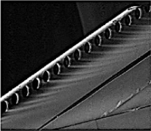
  $2.7\,\mathrm {\mu }$m. A Mitutoyo surface micrometer was used to verify the film thickness. A photograph of the cone model with the 3M film applied is shown in figure 3. The image also shows an example of the circular cut-outs in the black film near the fin leading edge that served as discrete roughness elements (DREs) used in transition control.
Photograph of the  $7^{\circ }$ half-angle cone with a $70^{\circ }$ swept fin when covered by matte black 3M film used for IR imaging. The image shows an example of the circular cut-outs in the black film near the fin leading edge that served as DREs.

An InfraTec ImageIR 8300 hp MWIR camera and a forward-looking IR (FLIR) SC8000 MWIR camera were used in imaging. The InfraTec camera was operated at  $640 \times 512$ pixel resolution at 355 frames per second (fps). The FLIR camera was operated at $1344 \times 784$ pixel resolution at 128 fps. Comparing thermal data from the two cameras revealed that the FLIR camera consistently recorded slightly higher temperatures than the InfraTec camera, by about 1 K. Given its higher resolution, all quantitative heating measurements were performed with the FLIR camera.
The thermal images from the FLIR camera were calibrated spatially and processed into heat flux data. Two-dimensional, cross-correlation-based image registration was used to account for model motion between thermograph frames. All frames from a run were aligned with a reference frame, which improved the accuracy and consistency of the heat flux calculations.
The conversion of the thermal images into heat flux was done using a modified version of the heat flux solver QCALC (Juliano et al. Reference Juliano, Poggie, Porter, Kimmel, Jewell and Adamczak2018). The solver uses finite-thickness, one-dimensional finite-difference approximations of the temporal and spatial derivatives in the one-dimensional heat equation (Boyd & Howell Reference Boyd and Howell1994). A first order Euler-explicit method is used to approximate the temporal derivative. A second-order Euler-explicit difference method was used to approximate the spatial derivative
 \begin{equation} \frac{\partial T}{\partial t} = \alpha\,\frac{\partial ^2 T}{\partial x^2} \end{equation}
into a discrete format
 \begin{equation} \frac{T_j^{i+1} - T_j^i}{{\rm \Delta} t} = \alpha\,\frac{T_{j+1}^i - 2T_j^i + T_{j-1}^i}{({\rm \Delta} x)^2}, \end{equation}
where  $\alpha$ is the thermal diffusivity of the material, $i$ is the temporal position, and $j$ is the spatial node in the image. An initial uniform temperature distribution throughout the surface was assumed. Based on the short (80 ms) run time, the thermal images set the film exposed-face boundary condition, while an isothermal film wall-contact face was assumed.
Two considerations went into the spatial discretization. The first was that at least three spatial nodes are required for the finite-difference approximation, so that  $3\,{\rm \Delta} x$ could not exceed the thickness of the matte black film. The second constraint is the stability criterion, ${\rm \Delta} x \geq \sqrt {2 \alpha \,{\rm \Delta} t}$. Here, ${\rm \Delta} t$ is set by the frame rate of the camera, and $\alpha$ is assumed constant. This put a lower bound on the node spacing. With the error in the second-order finite-difference approximation being proportional to $({\rm \Delta} x)^2$, the object was to minimize ${\rm \Delta} x$ without violating the stability criterion.
To account for wall temperature variations between experimental runs, the Stanton number was computed, where
 \begin{equation} St=\frac{Q_w}{\rho_{\infty}U_{\infty} c_p(T_0-T_w)}, \end{equation}
in which  $Q_w$ is the surface heat flux, $\rho _{\infty }$ is the free-stream air density, $U_{\infty }$ is the free-stream velocity, $T_w$ is the wall temperature, and $T_0$ is the stagnation temperature.
There are several sources of error in the IR-based heat flux imaging. The FLIR camera manufacturer states that the camera margin of error for a properly calibrated system is  ${\pm }1\,^{\circ }$C or 1 % of readings. In addition, there is the issue of the image transmission to the camera. The heat flux data were computed from images where the camera was placed at angles $5\unicode{x2013}10^{\circ }$ with respect to the fin-normal direction. Running et al. (Reference Running, Rataczak, Zaccara, Cardone and Juliano2022) found that the emissivity of the 3M film had a value near 0.95 within this viewing angle range, with value 1 indicating an idealized black body source. Finally, the FLIR camera lists its spectral band to be $1.5\unicode{x2013}5\,\mathrm {\mu }$m. The imaging window for these experiments was sapphire, which has an optical transmission value near 90 % in the $1\unicode{x2013}4\,\mathrm {\mu }$m range, but begins to drop sharply for wavelengths above $5\,\mathrm {\mu }$m.
The film density, thermal conductivity and specific heat from Running et al. (Reference Running, Rataczak, Zaccara, Cardone and Juliano2022) are listed in table 2. The air density and free-stream velocity were computed based on the isentropic flow relation with the stagnation temperature and pressure given in table 1. Based on these listed values, the estimated uncertainty in the absolute Stanton number is  ${\pm }8\,\%$.
3M film properties (Running et al. Reference Running, Rataczak, Zaccara, Cardone and Juliano2022).

In addition to the heat flux measurements, the fin was instrumented with four Kulite XCS-062 5 absolute pressure sensors. The arrangement of the pressure transducers on the fin is shown in figure 4. The four transducers were arranged in a square array spaced 2.54 mm on centres apart. The location of each pair of transducers is measured from the line where the fin round leading edge is tangent to the flat fin surface. This then corresponds to 3.175 mm from the fin leading edge. The pressure sensor locations generally bracketed where turbulence onset occurred on the fin surface.
Schematic drawing showing the locations array of four Kulite XCS-062 5 pressure sensors that were flush mounted in the swept fin. Dimensions are in mm.

The Kulite sensors were calibrated in situ using a reference static pressure sensor located in the tunnel vacuum tank. Pressure measurements were acquired as the test section was pumped down in pressure. A linear curve fit was then performed on the voltage–pressure data pairs. The analogue output from the sensors was analogue frequency compensated to extend the nominally 30 kHz frequency response (flat to  ${\pm }3$ dB) to encompass the expected frequency range of the travelling cross-flow modes. A test of the sensor response with the compensation circuit in a shock tube verified the frequency response to be up to 150 kHz. An analogue fourth-order low-pass filter with cut-off frequency 150 kHz was used as an anti-alias filter to the pressure time series that was acquired at 300 kHz. Details of the circuit design and experimental frequency response are available from Middlebrooks (Reference Middlebrooks2023b).
The experiment was performed at three unit Reynolds numbers for three nose radii. The conditions for the experiment are listed in table 3. The lowest unit Reynolds number, 11 M m $^{-1}$ (3.34 M ft $^{-1}$), matched the conditions of Turbeville & Schneider (Reference Turbeville and Schneider2018) and Knutson et al. (Reference Knutson, Sidharth and Candler2018). The highest unit Reynolds number with the largest nose radius was expected to result in neutral growth of the second mode (Paredes et al. Reference Paredes, Choudhari, Li, Jewell, Kimmel, Marineau and Grossir2018; Batista & Kuehl Reference Batista and Kuehl2019) on the cone frustum.
Experimental conditions.
 $^{1}$Matches conditions of Knutson et al. (Reference Knutson, Sidharth and Candler2018) and Turbeville & Schneider (Reference Turbeville and Schneider2018). $^{2}$Expected (Paredes et al. Reference Paredes, Choudhari, Li, Jewell, Kimmel, Marineau and Grossir2018; Batista & Kuehl Reference Batista and Kuehl2019) to produce neutral second mode growth on cone frustum.
3. Results
The initial experiments used a smooth fin, free of roughness elements, allowing for natural transition to occur. These cases provided the baseline heating distributions for the discrete roughness experiments. Figure 5(a) shows an example of an IR image taken during one of the tunnel runs at  $Re_{unit}=22$ M m $^{-1}$ and the largest nose radius, $r_n=5.33$ mm. Figure 5(b) corresponds to the computed surface heat flux based on the IR image in figure 5(a). Both the surface temperature and heat flux images of the cone fin reveal clearly hot and cold streaks that are indicative of stationary cross-flow modes.
(a) Sample IR surface temperature image and (b) computed surface heat flux of the fin portion of the model taken during a tunnel run at  $Re_{unit}=22$ M m $^{-1}$ with $r_n=5.33$ mm cone tip.

The stationary pattern believed to be the result of stationary cross-flow vortices was most apparent in the IR images of the higher unit Reynolds number cases, although detailed analysis of the spatial IR intensity values would reveal their presence even at the lowest unit Reynolds number, 11 M m $^{-1}$. A review of the thermal images from Turbeville & Schneider (Reference Turbeville and Schneider2018, Reference Turbeville and Schneider2019) does not reveal evidence of cross-flow vortices on the fin. There are a number of possible reasons. One is that their temperature-sensitive paint was not as sensitive as the present IR images. Another is that their experiments were conducted in a ‘quiet’ tunnel with lower disturbance levels. However, as discussed in § 1, stationary cross-flow modes are highly insensitive to free-stream disturbance levels. Therefore, the most likely difference is in the Reynolds numbers. A majority of the Turbeville & Schneider (Reference Turbeville and Schneider2018, Reference Turbeville and Schneider2019) experiments were conducted at $Re_{unit} \leq 8.12$ M m $^{-1}$. That, compounded by them having a 40 % shorter model, lowered the streamwise Reynolds number. Based on the present observations, this is likely the central difference that made it possible to visualize the stationary cross-flow vortices under baseline conditions.
In order to perform quantitative analysis, the surface heat flux values were sampled from the respective images. Figure 6(a) shows a colour rendering of the heat flux that was reconstructed from the heat flux image shown in figure 5(b). The mean heat flux has been subtracted from the individual values in order to highlight the stationary heat flux features. These data again correspond to the baseline (smooth) fin with the  $r_n=5.3$ mm cone tip at $Re_{unit}=22$ M m $^{-1}$.
(a) Example of reconstructed heat flux obtained from sampling digital heat flux image, showing coordinate system, and (b)  $St\,Re^{1/2}$ profiles measured in lines perpendicular to the fin leading edge and averaged over the area parallel to the leading edge. Conditions are baseline (smooth) fin with the $r_n=5.3$ mm cone tip at $Re_{unit}=22$ M m $^{-1}$.

Figure 6(a) includes the coordinate system used in figure 6(b) and in subsequent figures. The coordinate  $x_{\perp }$ is drawn perpendicular to the fin leading edge, with $x_{\perp }=0$ at the leading edge. The coordinate $x_{\parallel }$ is drawn to be parallel to the fin leading edge. Its origin is arbitrary.
Reconstructed heat flux images like the one shown in figure 6(a) were then used to quantify the development of the boundary layer over the fin. This involved measuring profiles along lines perpendicular to the leading edge of the fin surface heat flux that were averaged over an area parallel to the leading edge. The result for the baseline (smooth) fin with the  $r_n=5.3$ mm cone tip at $Re_{unit}=22$ M m $^{-1}$ is shown in figure 6(b). For this, the heat flux is represented by the commonly used product of the Stanton number and the unit Reynolds number, namely $St\,Re^{1/2}$. The Stanton number accounts for differences in the initial surface temperature, which can vary with each wind tunnel run. The scaling by $Re^{1/2}$ has been shown to collapse laminar boundary layer heating values.
The profiles of  $St\,Re^{1/2}$ shown in figure 6(b) correspond to three different wind tunnel runs spaced over multiple days. The average of these three runs is shown by the dashed profile. The vertical bar represents the ${\pm }8\,\%$ uncertainty in the absolute Stanton number calculation described in § 2. This average profile will be used for comparison to other cases having discrete roughness. Of particular interest to these profiles is the boundary layer transition location, and location of turbulence onset. These are indicated in the plot as $x_{tr}$ and $x_T$, respectively. The transition location $x_{tr}$ is defined as the location where the heat flux begins to rise from the lower laminar values. The turbulence onset location $x_T$ is defined as the location where the heat flux peaks. For the baseline (smooth) fin, these two locations are at $x_{\perp }=8.5$ and 20 mm, respectively.
Figure 7 shows  $St\,Re^{1/2}$ profiles for the baseline (smooth) fin with the most sharp ( $r_n=0.15$ mm) and most blunt ( $r_n=5.3$ mm) cone nose tips at the lowest ( $Re_{unit}=11$ M m $^{-1}$) and highest ( $Re_{unit}=22$ M m $^{-1}$) unit Reynolds numbers used in the experiment. The profile corresponding to ‘blunt 22 M m $^{-1}$’ is the average profile from figure 6. The profiles for the other cases are similarly averages over multiple runs.
Normalized heat flux profiles for the baseline (smooth) fin measured in lines perpendicular to the fin leading edge and averaged over the area parallel to the leading edge for  $r_n=0.15$ mm (sharp) and $r_n=5.3$ mm (blunt) cone nose tips at $Re_{unit}=11$ and 22 M m $^{-1}$.

At either fixed Reynolds number, the effect of cone nose bluntness was small, with a slight increase in  $x_{tr}$ and $x_T$ with the blunt cone tip compared to the sharp tip. The major effect on $x_{tr}$ and $x_T$ was with Reynolds number, where both locations moved closer to the fin leading edge with increasing Reynolds number, and subsequently resulted in an overall increase in the surface heat flux.
As it has the largest spatial change in surface heat flux of the four cases, the remainder of the paper focuses on the case with the largest cone nose bluntness,  $r_n=5.3$ mm, and the highest unit Reynolds number, $Re=22$ M m $^{-1}$. Analysis of the other cases is available from Middlebrooks (Reference Middlebrooks2023a).
The design of the discrete roughness for cross-flow transition control requires knowing the predominant wavelengths of stationary cross-flow modes. Wavelet analysis was therefore performed on the reconstructed surface heat flux data for the baseline case with  $r_n=5.3$ mm at $Re=22$ M m $^{-1}$ that was shown in figure 6 in order to determine the predominant wavelengths of stationary features that are presumed to correspond to stationary cross-flow modes. The results are shown in figure 8. These correspond to three locations relative to the fin leading edge: one close to the fin leading edge at $x_{\perp }=3$ mm, one further from the leading edge at $x_{\perp }=8$ mm, which is approximately $x_{tr}$, and one still further from the leading edge at $x_{\perp }=16$ mm, which is slightly upstream of $x_T$.
Sample wavelet results for extracted heat flux data lines in the  $x$-direction parallel to the leading edge at three distances from the fin leading edge $y_{LE}$ for a cone nose with $r_n=5.3$ mm at $Re_{unit}=22$ M m $^{-1}$.

Close to the fin leading edge at  $x_{\perp }=3$ mm, the wavelet analysis indicates energy that is predominantly in smaller wavelengths, with the shortest wavelength being approximately 2 mm. Wavelengths 2–3 mm were predicted to be the most amplified close to the fin leading edge based on linear stability analysis of Peck et al. (Reference Peck, Mullen, Reed, Turbeville and Schneider2022b). However, as the boundary layer develops from the fin leading edge, the wavelet analysis indicates that the predominant wavelength shifts towards larger values. At $x_{\perp }=8$ mm, which is close to $x_{tr}$, the predominant wavelength is approximately 10–12 mm. Further from the fin leading edge at $x_{\perp }=16$ mm, which is slightly upstream of $x_T$, the predominant wavelengths are 12–15 mm.
Two-dimensional ( $x_{\perp }$ by $x_{\parallel }$) spectral analysis of the spatial heat flux pattern was also used to quantify the wavelengths of stationary features (Middlebrooks Reference Middlebrooks2023a). These were then used to document the $x_{\perp }$ development of these features based on their contribution to the surface heat flux. An example for the baseline (smooth) fin for a cone nose with $r_n=5.3$ mm and $Re_{unit}=22$ M m $^{-1}$ is shown in figure 9. In this, the development of stationary features at five discrete wavelengths ranging from 6 to 16 mm is presented. For reference, the locations of $x_{tr}$ and $x_T$ for this case, taken from figure 6, are noted on the figure.
Development of different wavelengths of heat flux pattern over the baseline (smooth) fin surface for a cone nose with  $r_n=5.3$ mm at $Re_{unit}=22$ M m $^{-1}$.

Figure 9 shows that the significant growth of larger wavelengths of stationary features in the heat flux on the fin occurs close to  $x_{tr}$. The largest growth occurs with wavelengths 8–12 mm.
The information gained from the wavelet analysis and wavelength development were used to design a DRE for cross-flow transition control. The method of cross-flow transition control involves raising the initial amplitude of less-amplified cross-flow modes so that initially they dominate instability growth. The growth of the forced modes is intended to inhibit the growth of the more amplified (‘critical’ wavelength; Saric et al. Reference Saric, Ruben and Reibert1998b) stationary modes by modifying the basic state. Ultimately, the forced modes will result in turbulence onset. However, in experiments at Mach 3.5 (Schuele et al. Reference Schuele, Corke and Matlis2013) and at Mach 6 (Corke et al. Reference Corke, Arndt, Matlis and Semper2018; Arndt et al. Reference Arndt, Corke, Matlis and Semper2020), the approach has been successful in delaying turbulence onset by as much as 40 %. In the present experiments, the delay in turbulence onset is motivated by the objective to reduce surface heat flux. This remains as a metric of success.
Following our previous approach to cross-flow transition control (Schuele et al. Reference Schuele, Corke and Matlis2013; Corke et al. Reference Corke, Arndt, Matlis and Semper2018; Arndt et al. Reference Arndt, Corke, Matlis and Semper2020), surface recesses (‘dimples’) were used as the DREs. These have the advantage of uniformity in size and depth. The criterion (Saric, Carrillo & Reibert Reference Saric, Carrillo and Reibert1998a; Radeztsky et al. Reference Radeztsky, Reibert and Saric1999) for the design of discrete roughness is that their wavelength be approximately 67 % smaller or larger than the critical wavelength. Another requirement borne out by our previous work is that the ratio of the roughness diameter  $d$ to roughness centre-to-centre spacing, $\lambda$, be $d/\lambda \geq 0.5$ (Radeztsky et al. Reference Radeztsky, Reibert and Saric1999). As has been typical on our previous experiments (Schuele et al. Reference Schuele, Corke and Matlis2013; Corke et al. Reference Corke, Arndt, Matlis and Semper2018; Arndt et al. Reference Arndt, Corke, Matlis and Semper2020) $d/\lambda \sim 0.5$.
Based on the wavelength distributions in figure 8, we focused on two ‘critical’ wavelengths, one in the range 2–3 mm close to the fin leading edge, and the other in the range 8–12 mm that appeared to be dominant further from the leading edge near  $x_{tr}$. Given these wavelengths, in the first set of experiments, the diameter of the roughness was chosen to satisfy the $d/\lambda \geq 0.5$ criteria. The effect of $d/\lambda$ follows. The parameters of the discrete roughness are given in table 4. In all cases, the depth of the roughness cut-outs was fixed at 112.3 $\mathrm {\mu }$m. Although it is not presented here, Middlebrooks (Reference Middlebrooks2023a) also examined the effect of the depth of the roughness recesses.
Discrete roughness properties.

The roughness recesses were generated by laser-cutting circular holes in the 3M film that was placed over the fin for the IR measurements. The film is glue-backed and attached initially to a backing sheet. When the backing sheet was removed, the laser-cut holes remained on the backing sheet to leave openings in the film corresponding to the hole locations. An example of the circular cut-outs in the black film near the fin leading edge was shown in the cone image in figure 3. The holes reveal the metal surface of the swept fin. In these cases, the depth of the discrete roughness holes is the thickness of the film, 112.3  $\mathrm {\mu }$m.
The first set of results correspond to the initially smaller wavelengths that were observed to occur close to the leading edge and were predicted from linear theory. For this, the ‘critical’ wavelength was considered to be 2 mm. Following the DRE design approach (Saric et al. Reference Saric, Carrillo and Reibert1998a; Radeztsky et al. Reference Radeztsky, Reibert and Saric1999), discrete roughnesses were chosen with subcritical wavelength  $\lambda =1.7$ mm and supercritical wavelength $\lambda =2.6$ mm. Figure 10 shows an image of the fin surface heat flux, the corresponding wavelet analysis at $x_{\perp }=5$ mm (middle) and the development of different wavelengths in the stationary heat flux pattern with discrete roughness having $\lambda =1.7$ mm. These can respectively be compared to the values for the baseline (smooth) fin that were shown in figures 5, 8 and 9.
(a) Heat flux image, (b) corresponding wavelet analysis at  $x_{\perp }=5$ mm, and (c) development of different wavelengths in the stationary heat flux pattern over the fin surface with discrete roughness with $\lambda =1.7$ mm and $d/\lambda =0.5$ for a cone nose with $r_n=5.3$ mm at $Re_{unit}=22$ M m $^{-1}$.

Comparing the surface heat flux image to that for the smooth fin shows a more regular pattern of the hot and cold streaks that result from the discrete roughness. The corresponding wavelet analysis measured at  $x_{\perp }=5$ mm from the leading edge does not show significant magnitude at the 1.7 mm wavelength. Finally, the development of different wavelengths in the stationary heat flux pattern is remarkably similar to that of the smooth fin. Collectively, it would appear that the $\lambda =1.77$ mm wavelength DRE did not have a significant effect on the stationary cross-flow mode development.
For comparison to the  $\lambda =1.7$ mm wavelength case, figure 11 shows an image of the fin surface heat flux image, the corresponding wavelet analysis at $x_{\perp }=5$ mm (middle) and the development of different wavelengths in the stationary heat flux pattern with discrete roughness having $\lambda =2.6$ mm. The surface heat flux image shows a more clear pattern of hot and cold streaks. The wavelet analysis measured at $x_{\perp }=5$ mm from the fin leading edge reveals a 2 mm wavelength band with a magnitude that is well above the background. The most notable difference from the $\lambda =1.7$ mm wavelength case comes in comparing the development of different wavelengths in the stationary heat flux pattern, which is dramatically different to that of the smooth fin case. In particular, the peak amplitudes have moved closer to the fin leading edge, with the largest wavelength being $\lambda =18$ mm, which dominates the wavelengths.
(a) Heat flux image, (b) corresponding wavelet analysis at  $x_{\perp }=5$ mm, and (c) development of different wavelengths in the stationary heat flux pattern over the fin surface with discrete roughness with $\lambda =2.6$ mm and $d/\lambda =0.5$ for a cone nose with $r_n=5.3$ mm at $Re_{unit}=22$ M m $^{-1}$.

Figure 12 provides a global picture of the effect of the discrete roughness at the two wavelengths. This shows the normalized heat flux profiles taken in the direction perpendicular to the fin leading edge and averaged in the direction parallel to the leading edge. Again, for reference, the profile for the baseline (smooth) fin is shown. We consider two effects of the discrete roughness. One is to delay either  $x_{tr}$ and/or $x_T$. The other is more specific to the practical motivation, which is to lower the surface heat flux on the fin. With regard to the first effect, neither of the two discrete roughness wavelengths had a significant effect on $x_{tr}$. In contrast, both reduced $x_T$ compared to the baseline. With regard to the second effect, both of the discrete roughness wavelengths reduced the surface heat flux, with the largest reduction occurring with $\lambda =2.6$ mm. However, lacking the delay in $x_{tr}$, the mechanism for the heat flux reduction does not follow the linear stability norms on which the DRE approach is based.
Normalized heat flux profiles measured in lines perpendicular to the fin leading edge and averaged over the area parallel to the leading edge for a fin with discrete roughness having  $\lambda =1.7$ and 2.6 mm with $d/\lambda =0.5$ for a cone nose with $r_n=5.3$ mm at $Re_{unit}=22$ M m $^{-1}$.

As noted in the wavelet analysis that was shown in figure 8 for the baseline (smooth) fin, the predominant wavelengths of stationary heat flux patterns shifted to longer wavelengths near the location of  $x_{tr}$. The development of different wavelengths in the stationary heat flux pattern indicated that the dominant wavelengths were in the range 8–12 mm. Given this range, the middle 10 mm was designated to be the ‘critical’ wavelength. Then following the DRE design approach (Saric et al. Reference Saric, Carrillo and Reibert1998a; Radeztsky et al. Reference Radeztsky, Reibert and Saric1999), the subcritical wavelength was $\lambda =6.7$ mm, and the supercritical wavelength was $\lambda =13.3$ mm.
The results for the  $\lambda =6.7$ mm wavelength discrete roughness are shown in figure 13. The image of the surface heat flux shows an extremely clear pattern of hot and cold streaks that line up perfectly with the roughness elements. This is further supported by the wavelet analysis that shows the 6.7 mm wavelength to be dominant. This is further reenforced in the development of the different wavelengths of stationary features in the heat flux where the largest amplitude is at 6 mm (nominally the discrete roughness wavelength). The 6 mm wavelength remains the largest to $x_{\perp } =20$ mm, which is an important observation in evaluating the effectiveness of the different roughness wavelengths.
(a) Heat flux image, (b) corresponding wavelet analysis at  $x_{\perp }=5$ mm, and (c) development of different wavelengths of in the stationary heat flux pattern over the fin surface with discrete roughness with $\lambda =6.7$ mm and $d/\lambda =0.5$ for a cone nose with $r_n=5.3$ mm at $Re_{unit}=22$ M m $^{-1}$.

In contrast to the results with the  $\lambda =6.7$ mm wavelength discrete roughness, figure 14 shows results with the $\lambda =10$ mm roughness. Starting with the image of the surface heat flux, the pattern is not as regular as with the $\lambda =6.7$ mm case. In particular, there appears to be a longer-wavelength $x_{\parallel }$ variation that was not apparent in the previous case. Similarly in contrast to the $\lambda =6.7$ mm case, the 10 mm roughness wavelength is not apparent in the wavelet analysis. Instead there is recognition of a 5 mm wavelength that might be a subharmonic of the discrete roughness wavelength. Most notable is evidence of long wavelengths ranging from 11–16 mm that were prominent in the baseline (smooth) fin case. Finally, in contrast to the previous $\lambda =6.7$ mm case, the development of the different wavelengths of stationary features in the heat flux shows no dominant wavelength.
Heat flux image (a), corresponding wavelet analysis at  $x_{\perp }=5$ mm (b) and development of different wavelengths of in the stationary heat flux pattern over fin surface (c) with discrete roughness with $\lambda =10$ mm and $d/\lambda =0.5$ for a cone nose with $r_n=5.3$ mm, and at $Re_{unit}=22$ M m $^{-1}$.

The last case in this group corresponds to discrete roughness wavelength  $\lambda =13.3$ mm. This is shown in figure 15. The image of the surface heat flux shows a regular pattern similar to that of the $\lambda =6.7$ mm case. The wavelet analysis indicates that the 13.3 mm wavelength is dominant. A subharmonic wavelength is also appearing. The most telling result is in the development of the different wavelengths of stationary features in the heat flux. There, the 13 mm wavelength is not only dominant, but it remains dominant throughout the measured $x_{\perp }$ range. This is the desired effect and the basis of the discrete roughness transition control approach. We also note that the maximum amplitude of $St/St_{min}$ with the $\lambda =13.3$ mm roughness is notably less than that in the other two cases, and comparable to that in the baseline (smooth) case that was shown in figure 9. This is also a key point to the discrete roughness design.
(a) Heat flux image, (b) corresponding wavelet analysis at  $x_{\perp }=5$ mm, and (c) development of different wavelengths of in the stationary heat flux pattern over the fin surface with discrete roughness with $\lambda =13.3$ mm and $d/\lambda =0.5$ for a cone nose with $r_n=5.3$ mm at $Re_{unit}=22$ M m $^{-1}$.

The final judgement on the effect of the three wavelength cases of the discrete roughness comes from the overall effect on the normalized heat flux profiles taken in the direction perpendicular to the fin leading edge and averaged in the direction parallel to the leading edge. This is shown in figure 16. Here again, the important metrics are delaying either  $x_{tr}$ and/or $x_T$, and a lowering of the surface heat flux on the fin. Again for reference, the profile for the baseline (smooth) fin is included in the plot.
Normalized heat flux profiles measured in lines perpendicular to the fin leading edge and averaged over the area parallel to the leading edge for a fin with discrete roughness having  $\lambda =6.7$, 10 and 13.3 mm for a cone nose with $r_n=5.3$ mm at $Re_{unit}= 22$ M m $^{-1}$.

Of the three discrete roughness cases, only the supercritical  $\lambda =13.3$ mm wavelength case met both metrics by both delaying transition, and significantly reducing the overall surface heat flux. The other two roughness wavelengths actually reduced $x_{tr}$, compared to the baseline, and as a result increased the overall surface heat flux on the fin.
All of the previous cases used discrete roughness in which  $d/\lambda =0.5$. Therefore, an investigation of the effect of $d/\lambda$ was performed. For this, the most effective discrete roughness $\lambda = 13.3$ mm was kept fixed, and the diameter $d$ was varied. Two cases were examined, corresponding to $d/\lambda =0.25$ and 0.75. The results in terms of the overall effect on the normalized heat flux profiles taken in the direction perpendicular to the fin leading edge and averaged on the direction parallel to the leading edge are shown in figure 17. For reference, the profile from the previous $d/\lambda =0.5$ is shown in the plot for comparison.
Normalized heat flux profiles measured in lines perpendicular to the fin leading edge and averaged over the area parallel to the leading edge for a fin with discrete roughness having  $d/\lambda =0.25$, 0.5 and 0.75 for a cone nose with $r_n=5.3$ mm at $Re_{unit}=22$ M m $^{-1}$.

Comparing the three cases having a  $\lambda =13.3$ mm wavelength, there is a decided effect of the discrete roughness $d/\lambda$. The cases with $d/\lambda =0.25$ and 0.75 both delayed $x_{tr}$ by an amount that was comparable to the previous $d/\lambda =0.5$. The $d/\lambda =0.25$ case resulted in a minimum reduction in the overall surface heat flux. This occurred just following $x_{tr}$. In contrast, the $d/\lambda =0.75$ case showed a significant reduction in the overall surface heat flux. In this case, as indicated in table 4, the diameter of the discrete roughness was 50 % larger than when $d/\lambda =0.5$. This might have produced a ‘shielding effect’, widening the lower heat flux regions, and narrowing the higher heat flux regions between the discrete roughnesses. Evidence of this effect appears in the surface heat flux images, particularly for the larger wavelength roughness in figures 13 and 15.
3.1. Large wavelength stationary mode development
The results indicated that although shorter wavelengths of stationary patterns in the surface heat flux were evident near the fin leading edge, the dominant wavelengths of stationary patterns further from the fin leading edge, and prior to turbulence onset, were significantly larger. It is presumed that the stationary patterns in the surface heat flux are evidence of stationary cross-flow modes. As pointed out, in linear stability analysis for our experimental conditions (Peck et al. Reference Peck, Mullen, Reed, Turbeville and Schneider2022b), the most amplified wavelengths of stationary cross-flow modes near the fin leading edge were in the observed range 2–3 mm. Therefore, what is the source for the development of the longer wavelengths prior to turbulence onset?
In experiments of cross-flow instability on a rotating disk, Corke & Knasiak (Reference Corke and Knasiak1998) had documented a triad resonance between stationary and travelling cross-flow modes. This was found (Matlis Reference Matlis1997; Corke et al. Reference Corke, Matlis and Othman2007) to lead to the growth of low azimuthal stationary cross-flow modes prior to turbulence onset. Similar observations of an interaction between travelling and stationary cross-flow modes were found on right-circular cones at angles of attack at Mach 3.5 (Schuele et al. Reference Schuele, Corke and Matlis2013) and at Mach 6 (Corke et al. Reference Corke, Arndt, Matlis and Semper2018; Arndt et al. Reference Arndt, Corke, Matlis and Semper2020). All of these led to interactions that resulted in low wavenumber (large wavelength) stationary cross-flow modes.
As a first step in determining if the large-wavelength stationary features in the surface heat flux were the result of an interaction between stationary and travelling cross-flow modes, it was necessary to detect travelling disturbances in the boundary layer on the fin. This was the purpose of the square array of pressure sensors located on the swept fin.
An example of the simultaneously sampled mean-removed pressure time series from sensors 3 and 1 for the sharp tip cone ( $r_n=0.15$ mm) at $Re_{unit}=11$ M m $^{-1}$ is shown in figures 18(a,b). The amplitude scales of the two plots are the same to illustrate the substantial increase in the amplitude of the pressure fluctuations between sensor positions 3 and 1, which, as shown in figure 6(b), span the region of the steepest increase in the surface heat flux. Figure 18(c) is the linear coherence between the two time series from the two sensors. A high linear coherence signifies linear phase locking, which is a necessary requirement to validate the phase angle between the two time series at a particular frequency. The peak in the coherence at 60 kHz was verified to be noise, as it appeared even without flow. The source was unknown. The other peaks can be traceable to the flow field.
(a,b) An example of the mean-removed pressure time series from sensors 3 and 1, respectively. (c) Linear coherence for the sharp tip cone with  $r_n=0.15$ mm at $Re_{unit}=11$ M m $^{-1}$. (d) The geometry used in determining cross-flow mode wavelength, phase speed and wave angles.

Only three simultaneously sampled sensor time series are needed to determine the wavelength, wave angle and phase speed of travelling cross-flow modes. Having four offers a level of redundancy to determine the uncertainty in the values. A schematic of the geometry used in analysing the phase differences between pressure sensors in the array is shown in figure 18(d).
Cross-spectral analysis was performed to determine the phase difference between frequencies in the time series at the different spatial locations (3, 2 and 1) in which the linear coherence, signifying linear phase locking, was significant. In the analysis of the phase information, two right triangles were defined as shown in figure 18(d). The sides of the two triangles,  $\lambda _{23}$ and $\lambda _{21}$, are perpendicular to each other. The pair of parallel vertical lines represents an arbitrary travelling wave direction.
The interior angles of the two triangles are defined as  $\psi _{21}$ and $\psi _{23}$. From geometry,
 \begin{equation} \psi_{23}=\cos^{{-}1}\frac{\lambda_{23}}{s} \quad \mbox{and}\quad \psi_{21}=\cos^{{-}1}\frac{\lambda_{21}}{s}, \end{equation}
where, as drawn,
 \begin{equation} \psi_{23} = \psi_{21}. \end{equation}
Now the lengths  $\lambda$ are
 \begin{equation} \lambda_{23} = c_r\,\tau_{23}(f) = \frac{c_r\,\phi_{23}(f)}{360^{{\circ}}\,f} \quad \mbox{and}\quad \lambda_{21} = c_r\,\tau_{21}(f) = \frac{c_r\,\phi_{21}(f)}{360^{{\circ}}\,f}, \end{equation}
where  $c_r$ is the unknown phase speed of a travelling wave, and $\phi (f)$ is the phase difference (in degrees) at frequency $f$ measured by the two sensors. Substituting these into the expressions for $\psi$ gives the condition to determine the phase speed $c_r$, namely
 \begin{equation} \cos^{{-}1}\frac{c_r \phi_{23}}{360^{{\circ}}\,f s}=\cos^{{-}1}\frac{c_r \phi_{21}}{360^{{\circ}}\,f s}. \end{equation}
The phase speed  $c_r$ is that which satisfies the equality. Knowing the phase speed, the wavelength is $\lambda (f)=c_r/f$
There were a number of frequencies in the pressure time series that proved to be phase locked (high linear coherence) across the three sensors. These were verified to be in the flow field and not due to electronic noise or other facility-related disturbances. The frequencies that were linearly phase locked across the pressure sensors were generally either less than 5 kHz or greater than 90 kHz. Table 5 provides an example of both for the baseline (smooth) fin with the sharp ( $r_n=0.15$ mm) cone nose tip.
Sample of travelling disturbance characteristics determined from the pressure sensor array.

The sample low frequency was found to have a plausible phase speed ratio  $c_r/U_e=0.27$. Here, $U_e=792$ m s $^{-1}$ is the boundary layer edge velocity that was estimated using the Taylor–Maccoll solution for the post-cone shock conditions, and an oblique shock for the post-fin shock conditions. When converted to a wavelength, however, the value for the lower-frequency travelling disturbance was an implausibly large $\lambda =66.2$ mm. For reference, this is close to the maximum height of the fin. In contrast, the sample high-frequency travelling disturbance at $f=117.9$ kHz was determined to have a reasonable wavelength 6.9 mm, which is in the range of the stationary cross-flow modes. Its normalized phase speed was $c_r/U_e = 0.52$, and its wave angle was $\phi =14.4^{\circ }$.
It is possible that the lower-frequency travelling disturbances are due to the complex flow field that forms around the fin–cone junction. This is known to form a horseshoe vortex that could produce strong unsteadiness in the boundary layer on the fin (Tutty et al. Reference Tutty, Roberts and Schuricht2013). The lower frequency also appeared to be related to an amplitude modulation in the pressure time series at the furthest sensor locations that were close to the location of turbulence onset,  $x_T$.
3.1.1. Cross-bicoherence analysis
As discussed previously, close to the baseline (smooth) fin leading edge, the wavelet analysis indicated that the predominant wavelengths in the stationary heat flux pattern were of the order of 2–3 mm. It was pointed out that this agreed with predictions of the most amplified stationary cross-flow modes based on linear stability analysis (Peck et al. Reference Peck, Mullen, Reed, Turbeville and Schneider2022b). However, as the boundary layer developed from the leading edge, the wavelet analysis indicated that the predominant wavelength shifted towards larger values. For example, at  $x_{\perp }=8$ mm, which for the baseline fin is close to $x_{tr}$, the predominant wavelength was approximately 10–12 mm. Still further from the fin leading edge at $x_{\perp }=16$ mm, which is slightly upstream of $x_T$, the predominant wavelengths were 12–15 mm. In addition, DREs that were designed based on the larger wavelength performed the best in delaying transition and reducing the surface heat flux.
What is the mechanism that leads to the development of the larger wavelengths? Presuming that they are stationary cross-flow modes, their development is not predicted from linear stability analysis. Previous experiments on cones at an angle of attack at Mach 6 (Corke et al. Reference Corke, Arndt, Matlis and Semper2018; Arndt et al. Reference Arndt, Corke, Matlis and Semper2020) documented evidence of a quadratic interaction between the stationary and travelling cross-flow modes. This followed from previous experiments that documented a quadratic interaction between cross-flow modes in the boundary layer over a rotating disk (Matlis Reference Matlis1997; Corke & Knasiak Reference Corke and Knasiak1998; Corke et al. Reference Corke, Matlis and Othman2007). The quadratic interaction was determined to lead to low-wavenumber (large-wavelength) stationary cross-flow modes that emerged prior to turbulence onset.
In these previous experiments (Corke et al. Reference Corke, Arndt, Matlis and Semper2018; Arndt et al. Reference Arndt, Corke, Matlis and Semper2020), a quadratic interaction between modes was documented through the cross-bicoherence (CBC) statistic. The CBC is a measure of the phase locking between two frequencies in two time series, with a third frequency in one of the two time series. It is defined as
 \begin{equation} \beta_{ijk}(f_1,f_2) = \frac{|\tilde{R}_{ijk}(f_1,f_2) |^2}{\langle |\tilde{s}_i(f_1)|^2 |\tilde{s}_j(f_2)|^2\rangle \langle| \tilde{s}_k(f_3) |^2\rangle}, \end{equation}
where
 \begin{equation} \tilde{R}_{ijk}(f_1,f_2) = \langle\tilde{s}_i(f_1)\,\tilde{s}_j(f_2)\,\tilde{s}^*_k(f_3)\rangle \end{equation}
is the cross-bispectrum, with  $i$,
$i$,  $j$ and $k$ equal to either $i$ or $j$ that refer to one of the two mean-removed data (space or time) series $s$, with frequencies $f_1$, $f_2$ and $f_3$, respectively. The notation $|\cdot |$ is the modulus of the component, a tilde denotes the Fourier transformed function in the frequency domain, and $\langle \cdot \rangle$ represents the ensemble average. These frequencies are related to each other such that $f_1 + f_2 + f_3 =0$.
The value of the CBC varies between 0 and 1. High values of the CBC indicate a high degree of triple phase locking
 \begin{equation} \phi_i(f_1) + \phi_j(f_2) = \phi_k(f_3) \end{equation}
from realization to realization. Here,  $\phi _i(f_1)$ is the instantaneous circular phase angle of $\tilde {s}_i(f_1)$.
The region of validity of the CBC is set by the Nyquist criterion, where the sum of any two frequencies cannot exceed half the sampling rate. This region then takes the form of two isosceles triangles, one each for sum and difference interactions.
The CBC analysis was performed for the baseline swept fin cone with the sharp ( $r_n=0.15$ mm) tip at $Re_{unit}=11$ M m $^{-1}$. One of the data series is the reconstructed heat flux obtained by sampling the digital heat flux image. This is representative of the stationary features in the surface heat flux that are presumed to be tied to stationary cross-flow modes. This covers a region over the fin $6 \leq x_{\perp } \leq 32$ mm and $4 \leq x_{\parallel } \leq 90$ mm. These data are shown in figure 19. The second data series used in the CBC corresponds to the mean-removed pressure time series from pressure sensor 3 or 1. Examples of these were shown in figure 18.
Reconstructed mean-removed heat flux of swept fin on the cone with  $r_n=0.15$ mm at $Re_{unit}=11$ M m $^{-1}$ that was used in the CBC analysis.

In the CBC calculation, it is necessary that the two transformed data series have the same independent variable units. For the surface heat flux, the independent variable is wavelength  $\lambda$. With the pressure time series, the independent variable is frequency $f$. Therefore, in the case of the latter, we chose to convert frequency to wavelength. To do this, we used the phase speed $c_r=413.69$ m s $^{-1}$ that was found from the previously described linear phase analysis of the pressure sensor array time series.
Another important step in computing the CBC was that the sampling rates need to be the same for the two data series. For the data series representing the stationary cross-flow modes (surface heat flux), the sampling rate was 3.2 pixel-samples mm $^{-1}$. For the pressure time series, after conversion to wavelength, the sampling rate was 0.725 samples mm $^{-1}$. Therefore, in order to match the two data sampling rates, the surface heat flux data series was decimated by 4 to provide a closely matched sampling rate 0.80 pixel-samples mm $^{-1}$. The reconstructed heat flux image in figure 19 is the final, decimated surface heat flux used in the CBC analysis.
The decision about which of the two data series (1 or 2) corresponds to the  $i$,
$i$,  $j$ and $k$ series in the calculation of $\beta _{ijk}(f_1,f_2)$ in (3.5) is important. Here, we are seeking an explanation for the development of the larger wavelengths of the stationary patterns in the surface heat flux that are presumed to be evidence of stationary cross-flow modes. Based on the previous data, the transition to the larger wavelengths occurs in the distance from the fin leading edge $x_{\perp }$ that is between the locations of pressure sensors 3 and 1. It was also noted in figure 18 that the amplitude of the pressure fluctuations increased significantly between these two spatial locations.
With the objective of seeking a source for the development of the longer-wavelength stationary heat flux patterns at transition, the CBC shown in figure 20 has used a data series order that is designed to show quadratic phase locking of wavelengths in the stationary heat flux pattern (data series 1) with wavelengths in the travelling pressure disturbances at sensor 3 (data series 2), that through sum (upper triangle) and difference (lower triangle) interactions are phase locked to wavelengths in the travelling pressure disturbances at sensor 3 (data series 3). Thus we are seeking a mechanism where the stationary cross-flow modes could interact with the travelling cross-flow modes to produce other travelling cross-flow modes at different wavelengths. For reference, the corresponding auto-spectra of each data series are shown next to their respective axes. Note that the ‘frequency’ axes have units mm $^{-1}$ so that longer wavelengths are at the axes origin. The CBC levels are mapped to constant-level colour contours. Our focus is on the highest CBC levels, ${\geq }0.5$.
Cross-bicoherence showing quadratic phase locking at wavelengths between stationary features and travelling pressure disturbances at sensor 3 to wavelengths in the travelling pressure disturbances at sensor 3. The corresponding auto-spectra of each data series are shown next to their respective axes.

In figure 20, two different difference interactions and a summing interaction are highlighted. The method for reading the CBC is outlined by the arrows. Numbers have been added to the various interacting wavelengths to orient the reader. The interaction 1-2-3 is a difference interaction between a stationary feature [1], with an inverse wavelength 0.328 mm $^{-1}$, and a travelling disturbance [2], with an inverse wavelength 0.300 mm $^{-1}$ that is phase locked, with a travelling disturbance [3] having an inverse wavelength $0.328-0.300=0.028$ mm $^{-1}$, or wavelength $\lambda =35.7$ mm. The same wavelength stationary feature [1] is involved in a difference interaction with a travelling disturbance [7] with an inverse wavelength 0.035 mm $^{-1}$ that is phased locked with a travelling disturbance [8] having an inverse wavelength $0.328-0.035=0.293$ mm $^{-1}$, or wavelength $\lambda =3.4$ mm. An example of a summing interaction is 4-5-6, which involves a stationary feature [4], with an inverse wavelength 0.024 mm $^{-1}$, and a travelling disturbance [5], with an inverse wavelength 0.015 mm $^{-1}$ that is phase locked with a travelling disturbance [6] having an inverse wavelength $0.024+0.015=0.039$ mm $^{-1}$, or wavelength $\lambda =25.6$ mm. The question is if these could be a catalyst for the generation of the longer wavelength stationary modes that appear near turbulence onset. To presume to answer that, the CBC based on the pressure disturbances further from the fin leading edge, that were measured by sensor 1, is presented in figure 21.
Cross-bicoherence showing quadratic phase locking at wavelengths between travelling disturbances at sensor 1 and itself to wavelengths in the stationary features in the surface heat flux. The corresponding auto-spectra of each data series are shown next to their respective axes.

In simply comparing the CBC in figure 21 with the previous CBC in figure 20, the increase in the number of additional significant quadratic interactions is striking. The CBC shown in figure 21 has used a data series order that is designed to show quadratic phase locking of wavelengths in the travelling pressure disturbances (data series 1) with itself (data series 2) that through sum (upper triangle) and difference (lower triangle) interactions are phase locked to wavelengths in the stationary features in the surface heat flux (data series 3) that are presumed to be the result of stationary cross-flow modes. Thus here we are seeking a mechanism where the travelling cross-flow modes would interact with other travelling cross-flow modes to produce stationary cross-flow modes, particularly at longer wavelengths. Again for reference, the corresponding auto-spectra of each data series are shown next to their respective axes, and it is again noted that the ‘frequency’ axes have units mm $^{-1}$ so that longer wavelengths are at the axes origin. As before, the CBC levels are mapped to constant-level colour contours, and our focus is on the highest CBC levels, ${\geq }0.5$.
From figure 21, it is evident that as the boundary layer developed towards turbulence onset, the number of quadratic interactions among the travelling and stationary features increased. A number of these interactions are highlighted, with wavelengths denoted in the spectrum of the stationary heat flux features shown on the upper axis of the CBC. One in particular that is highlighted is labelled 1-2-3, which involves a summing interaction between a travelling disturbance [1] with an inverse wavelength 0.024 mm $^{-1}$ and a travelling disturbance [2] with an inverse wavelength $0.015$ m $^{-1}$ that is phase locked with a stationary feature [3] with an inverse wavelength $0.024+0.015=0.039$ mm $^{-1}$, or wavelength $\lambda =25.6$ mm, which is the wavelength of a travelling disturbance produced by the summing interaction 4-5-6 highlighted in the CBC in figure 20. The result of the CBC analysis suggests strongly that the longer-wavelength stationary wavelength patterns associated with stationary cross-flow modes that develop in the approach to turbulence onset are due to an interaction with travelling disturbances (cross-flow modes) in a manner similar to that observed previously in other cross-flow-dominated boundary layer flows (Matlis Reference Matlis1997; Corke & Knasiak Reference Corke and Knasiak1998; Corke et al. Reference Corke, Matlis and Othman2007, Reference Corke, Arndt, Matlis and Semper2018; Arndt et al. Reference Arndt, Corke, Matlis and Semper2020).
4. Conclusions
Experiments were performed to document the complex flow field around and over a  $70^{\circ }$ swept fin mounted on a $7^{\circ }$ half-angle right-circular cone in a Mach 6 free-stream. Of particular interest was the turbulent transition of the boundary layer over the swept fin, which was expected to be dominated by a cross-flow instability. Experiments were performed over a range of unit Reynolds numbers from 11 to 22 M m $^{-1}$. In addition, different cone frustum tips with nose radii ranging from $r_n=0.15$ to 5.33 mm, with the smaller radius at the lower Reynolds number, matched those in a previous experiment (Turbeville & Schneider Reference Turbeville and Schneider2018) and simulation (Knutson et al. Reference Knutson, Sidharth and Candler2018), with the larger nose radius expected (Paredes et al. Reference Paredes, Choudhari, Li, Jewell, Kimmel, Marineau and Grossir2018; Batista & Kuehl Reference Batista and Kuehl2019) to produce neutral second mode growth at the highest unit Reynolds number. The cone model was a 40 % larger version of the model used in those previous investigations (Knutson et al. Reference Knutson, Sidharth and Candler2018; Turbeville & Schneider Reference Turbeville and Schneider2018).
Stationary features consistent with stationary cross-flow modes were observed in infrared thermal images of the fin surface. These were processed further to determine average spatial Stanton number distributions over the fin. The  $St\,Re^{1/2}$ distributions revealed clearly locations of boundary layer transition $x_{tr}$ and turbulence onset $x_T$. At either fixed Reynolds number, the effect of cone frustum nose bluntness was small, with a slight increase in $x_{tr}$ and $x_T$ with the blunt cone tip compared to the sharp tip. The major effect on $x_{tr}$ and $x_T$ was with Reynolds number, where both locations moved closer to the fin leading edge with increasing Reynolds number, and subsequently resulted in an overall increased in the surface heat flux.
Wavelet analysis of the Stanton number distributions revealed stationary patterns with wavelengths near the fin leading edge that were consistent with linear theory predictions of stationary cross-flow modes. Further from the leading edge, the wavelength of the stationary patterns was observed to increase prior to turbulence onset. Achieving a possible explanation for the increase in the wavelength of the stationary patterns was one of the objectives.
Based on these observations, specially designed arrays of discrete roughness elements (DREs) were investigated as a means of delaying turbulence transition with the objective of reducing surface heat flux on the swept fin. The DRE designs followed our previous approach used for cross-flow transition control (Corke et al. Reference Corke, Arndt, Matlis and Semper2018; Arndt et al. Reference Arndt, Corke, Matlis and Semper2020). These focused on either the shorter wavelengths observed near the leading edge, or the longer wavelengths that developed near turbulence onset. In all cases, the DREs were always placed as close as possible to the fin leading edge.
The DREs that focused on the larger wavelengths of stationary modes were most effective at delaying transition and reducing the surface heat flux. Of these, the ratio of the diameter to centre-to-centre spacing that worked best was  $d/\lambda \geq 0.50$, which is consistent with DRE design norms of Saric et al. (Reference Saric, Carrillo and Reibert1998a) and Radeztsky et al. (Reference Radeztsky, Reibert and Saric1999).
A pressure sensor array located on the swept fin, flush with the fin surface, was used to document travelling disturbances that could include those associated with travelling cross-flow modes. Phase analysis of the pressure fluctuation time series was used to determine the wavelength, wave angle and phase speed that were consistent with the travelling cross-flow modes. The phase speed was used to convert the pressure time series to a wavelength data series that was used in the cross-bicoherence (CBC) analysis to determine quadratic interactions between the travelling disturbances and the stationary features in the surface heat flux that were presumed to be associated with stationary cross-flow modes.
The CBC analysis between the stationary and travelling disturbances indicated a nonlinear (quadratic) phase locking between the travelling disturbances and the stationary features in the surface heat flux. Of particular interest was whether this could explain the development of the larger wavelengths in the stationary features prior to turbulence onset. At a location on the fin close to  $x_{tr}$, the CBC indicated an interaction between short wavelengths of the stationary heat flux features associated with the linearly most amplified stationary cross-flow modes near the fin leading edge, and travelling disturbances with wavelengths close to those of the stationary features, that were quadratically phase locked to low-frequency, long-wavelength travelling disturbances.
Further from the fin leading edge, just upstream of  $x_T$, the long-wavelength travelling disturbances were subsequently found to be nonlinearly phase locked with a broad range of wavelengths of stationary features in the surface heat flux. These interactions are the suggested source of the development of the larger wavelengths of the stationary features in the surface heat flux during transition, consistent with previous observations of cross-flow transition (Matlis Reference Matlis1997; Corke & Knasiak Reference Corke and Knasiak1998; Corke et al. Reference Corke, Matlis and Othman2007, Reference Corke, Arndt, Matlis and Semper2018; Arndt et al. Reference Arndt, Corke, Matlis and Semper2020).
Of note is that one of the interactions involved a stationary wavelength 15 mm that was nominally close to the 13.33 mm wavelength of the discrete roughness that was most effective in delaying transition and lowering the heat flux on the swept cone. Since this longer stationary wavelength was involved in an interaction with travelling disturbances, it suggests a sensitivity to the wind tunnel disturbance levels that otherwise is not believed to be significant with stationary cross-flow modes. As a result, the degree to which cross-flow boundary layer transition and turbulence onset can be delayed using DREs may depend on the background disturbance levels.
Acknowledgements
We are grateful for the help provided by E. Farnan on the laser cutting of the black IR emission film that included the roughness element cut-outs.
Funding
The work was supported by the US Office of Scientific Research under grant N00014-19-1-2230, which was monitored by Dr E. Marineau. J.B.M. was supported in part through a Navy SMART Scholarship.
Declaration of interests
The authors report no conflict of interest.


 Open access