


1. Introduction
Tight control of minute microscopic scales, even close to the molecular scale, can be considered the key to many of today’s dominant technologies, ranging from pharmaceuticals, biochemistry or analytical chemistry to microelectronics. The fundamental step in realising such control always involves the ability to focus a stream of matter, be it a liquid, a gas or a photon beam, into a tightly controlled jet on a minute scale. When dealing with a liquid, focusing a differentiated stream of matter into a jet can be accomplished by several procedures involving a diversity of driving forces (Eggers & Villermaux Reference Eggers and Villermaux2008; Montanero & Gañán-Calvo Reference Montanero and Gañán-Calvo2020), which in almost all cases act against the surface tension of the liquid.
The action of focusing is ultimately associated with a conical geometry, where mass flow or energy reach a singularity at its apex. In exceptional occasions, a purely conical self-similar solution of the balance equations is discovered. Indeed, Buckmaster (Reference Buckmaster1972) criticised the much earlier proposal by Taylor (Reference Taylor1934), where the latter suggested that pointed-apex bubbles in a straining flow could develop a conical tip if the phenomenon is observed with sufficient resolution. That possibility was experimentally entertained by Rumscheidt & Mason (Reference Rumscheidt and Mason1961). However, Buckmaster showed a fact already noted by Taylor (Reference Taylor1966): that a conical flow around a capillary hollow cone is not possible fundamentally because the mechanical balance of surface stresses (normal and tangential stresses should vanish on the bubble surface) is impossible for a perfect conical shape. Eggers (Reference Eggers2021) obtained the complete non-conical solution to the problem of the strained bubble tip shape with finite curvature apex in the absence of emission, and showed it could be matched to Taylor’s theory as an outer solution.
A perfect balance of normal surface stresses in self-similar conical flows is only possible when every contributing normal stress scales identically with distance to the apex – so that surface tension is counteracted by an opposing stress of the same radial scaling. Exploiting this principle, conical Stokes-flow solutions driven by electrohydrodynamic forces have been developed (Ramos & Castellanos Reference Ramos and Castellanos1994; Gañán-Calvo & Montanero Reference Gañán-Calvo and Montanero2021), the canonical example being the electrostatic Taylor cone (Taylor Reference Taylor1964), where the liquid velocity is strictly zero. These solutions, however, possess an apex singularity: while the normal stresses can be exactly balanced at every radius, the local magnitudes diverge as the tip is approached. This divergence undermines strict self-similarity in real fluids, because the system resolves the singularity by emitting material from the apex. For Taylor’s solution the ensuing mass loss is the electrospray, whose ultimate scales depend on fluid properties. The enduring appeal of such conical states is precisely that they embed a geometric backbone mechanism for ‘focusing’, providing a natural pathway for concentrating stresses toward ever smaller scales.
Inspired by electrospray and using purely mechanical stresses, Gañán-Calvo (Reference Gañán-Calvo1998) demonstrated that a liquid stream can be focused into a tiny capillary jet by a converging gas flow. This method, known as flow focusing (FF), was later generalised to achieve the same focusing effect on a gas stream through a converging liquid flow (Gañán-Calvo & Gordillo Reference Gañán-Calvo and Gordillo2001). The most widely adopted FF configuration was introduced by Anna, Bontoux & Stone (Reference Anna, Bontoux and Stone2003), establishing a fundamental and enduring paradigm in microfluidics. More broadly, FF belongs to a classic class of fluid dynamics problems in which a given liquid volume undergoes stretching under a generalised extensional or focusing flow (Stone Reference Stone1994; Zhang Reference Zhang2004; Courrech du Pont & Eggers Reference Courrech du Pont and Eggers2006; Suryo & Basaran Reference Suryo and Basaran2006; Gañán-Calvo et al. Reference Gañán-Calvo, González-Prieto, Riesco-Chueca, Herrada and Flores-Mosquera2007; Eggers & Courrech du Pont Reference Eggers and Courrech du Pont2009; Eggers Reference Eggers2021). However, while an electrostatic field readily generates a conical potential that matches a surface-tension-held meniscus, so the system adopts the cone naturally without any imposed geometric constraint, the natural mechanical production of conical stresses has not yet been demonstrated unambiguously, even though substantial experimental and numerical indications point in that direction (Zhang Reference Zhang2004; Suryo & Basaran Reference Suryo and Basaran2006; Gañán-Calvo et al. Reference Gañán-Calvo, González-Prieto, Riesco-Chueca, Herrada and Flores-Mosquera2007; Dong et al. Reference Dong, Meissner, Faers, Eggers, Seddon and Royall2018; Courrech du Pont & Eggers Reference Courrech du Pont and Eggers2020; Rubio et al. Reference Rubio, Montanero, Eggers and Herrada2024). Establishing such a state would resolve a long-standing question: Can purely mechanical forcing sustain a local conical solution? In practical terms, it would imply the ability to control flow scales approaching those at which molecular interactions at free surfaces (e.g. disjoining pressure) are felt. At these near-molecular limits, FF enables extreme mixing and the emergence of macroscopic properties such as those found in ultra-fine emulsions (e.g. mayonnaise), despite the finite surface tension between the two phases.
1.1. Motivation and methodological approaches
We address a fundamental question in fluid physics arising from hydrodynamic focusing in the limit of a vanishing emitted flow rate: the existence of a local, self-similar conical flow structure that bridges two inherently distinct scales – a macroscopic domain influenced by non-conical boundary conditions, such as externally imposed extensional viscous flows, and a significantly smaller scale near the apex of the tapering meniscus. To address this problem, we develop two complementary approximations. The first employs general solutions of the Stokes equations in spherical coordinates, supplemented by numerical analysis to accurately capture the non-conical region that connects the self-similar cone to the emerging jet. In contrast, the second approach utilises slender-body lubrication theory, analytically capturing the complete cone-jet structure autonomously, provided the cone angle is sufficiently small. Remarkably, the lubrication theory yields a universal self-similar flow structure governed by a single dimensionless parameter directly linked to the extensional strength of the outer focusing fluid. Both solutions exhibit the same scaling dependency of the cone angle on the square root of the viscosity ratio between the inner and outer fluids. Ultimately, these two methods yield results in nearly perfect mutual agreement, with their correspondence becoming exact as the cone angle approaches zero. The predictions of these two approaches are systematically compared, where possible, with fully resolved numerical simulations available in the literature, in particular those reported in Rubio et al. (Reference Rubio, Montanero, Eggers and Herrada2024).
By analytically and numerically resolving this long-standing problem, we establish the feasibility of a locally conical, infinitely thinning flow geometry with virtually negligible emission, serving as an ideal intermediate asymptotic structure for forming perfectly cylindrical jets at extremely small scales. While our analysis is confined to scales above the onset of interfacial van der Waals effects (we do not include disjoining-pressure forces), understanding this limit is the necessary prerequisite for any future work that bridges the gap to true molecular-level phenomena. Our findings pave the way for technologies that require the precise manipulation of fluid flows at nearly molecular dimensions.
The first approach is structured in three steps.
-
(i) We first introduce an analytical conical flow solution of the Stokes equations as a local solution of FF or tip streaming in the limit of a zero emitted flow. This solution (see figure 1) is a modification of Buckmaster’s solution (Buckmaster Reference Buckmaster1972) to include the internal recirculating flow of the liquid inside the cone, which allows an exact balance of viscous stresses with surface tension at the cone surface with semi-angle $\alpha$
. Interestingly, this solution yields a constant velocity (independent of the spherical radial coordinate) at the cone surface. However, it requires the axis to be avoided in the external region due to the logarithmic singularity appearing there. Physically, the local flow around the axis emanating from the cone is akin to an infinitely thin ‘drawing line’ in the external flow moving the liquid from the tip of the cone to keep the flow running in the axial direction. Mathematically, the appearance of the logarithmic singularity at the axis in the flow outside the cone shows that a line of stokeslets at the axis must exist to keep the outer flow going in the form of an infinite conical configuration with a constant surface speed. Despite its obvious inconsistencies, this solution establishes the basis for a subsequent valid approximation: it is the extra degree of freedom at the axis that actually allows the existence of a conical solution, as illustrated next.
$\alpha$
. Interestingly, this solution yields a constant velocity (independent of the spherical radial coordinate) at the cone surface. However, it requires the axis to be avoided in the external region due to the logarithmic singularity appearing there. Physically, the local flow around the axis emanating from the cone is akin to an infinitely thin ‘drawing line’ in the external flow moving the liquid from the tip of the cone to keep the flow running in the axial direction. Mathematically, the appearance of the logarithmic singularity at the axis in the flow outside the cone shows that a line of stokeslets at the axis must exist to keep the outer flow going in the form of an infinite conical configuration with a constant surface speed. Despite its obvious inconsistencies, this solution establishes the basis for a subsequent valid approximation: it is the extra degree of freedom at the axis that actually allows the existence of a conical solution, as illustrated next. -
(ii) The above conical solution is supplemented with another inner solution that represents the jet and has constant flux to account for the emitted flow rate. This inner solution is approximately matched, at large distances from the cone-jet transition, with a solution considering an asymptotically cylindrical infinite jet with a diameter proportional to the local cone-jet transition scale.
-
(iii) The complete solution at the tip of the cone naturally entails the breakdown of the conical self-similar solution at the local scale of the cone-jet transition, which is the diameter of the emitted jet. At this scale, the conical shape tapers into a universal funnel shape that eventually turns into a perfectly cylindrical jet. This transition flow region is finally solved numerically for a given viscosity ratio and cone angle by Herrada’s method (Herrada & Montanero Reference Herrada and Montanero2016) using the proposed analytical flow solution as the asymptotic boundary condition.

Modified Buckmaster’s solution with inner flow field. The local spherical coordinates $R$
and
$R$
and $\theta$
are indicated, as well as domains 0 (inner) and 1 (outer stream). Here,
$\theta$
are indicated, as well as domains 0 (inner) and 1 (outer stream). Here, $\alpha$
is the cone semiangle and
$\alpha$
is the cone semiangle and $\mu _0$
and
$\mu _0$
and $\mu _1$
are the viscosities of the inner and outer incompressible fluids, respectively.
$\mu _1$
are the viscosities of the inner and outer incompressible fluids, respectively.

The second analytical method expands about the local flow strength at the axis of an arbitrary external axisymmetric flow governed by the Stokes equations. Using the slender-body approximation (see figure 2), a general formulation based on lubrication theory is developed, which is reduced to a similarity solution describing the cone-jet structure. This similarity solution is characterised by a single dimensionless parameter that represents the scaled external flow velocity at the point on the axis where the conical region transitions into a cylindrical thread. This governing parameter, defined as proportional to the square root of the viscosity ratio between the inner and outer fluids, exhibits a threshold below which stable conical solutions exist. This result is consistent with the predictions from the first approach: the threshold corresponds to the cone angle that maximises the interface velocity for the analytically exact solution, in the limit of vanishing viscosity ratio. Beyond this threshold, the solutions become non-conical (cusp-like).
The global FF geometry and the intermediate scale $l$
(
$l$
( $l_0 \ll l \ll l_\mu$
) where a conical geometry emerges. The cylindrical coordinates
$l_0 \ll l \ll l_\mu$
) where a conical geometry emerges. The cylindrical coordinates $\{r,z\}$
and the meniscus profile radius
$\{r,z\}$
and the meniscus profile radius $h(z)$
used in the slender-body theory are indicated. Here,
$h(z)$
used in the slender-body theory are indicated. Here, $\mu _0$
and
$\mu _0$
and $\mu _1$
are the viscosities of the inner and outer incompressible fluids, respectively. The macroscopic scale
$\mu _1$
are the viscosities of the inner and outer incompressible fluids, respectively. The macroscopic scale $R_0$
is imposed by any external boundary condition (here, a feeding tube), while the intermediate scale
$R_0$
is imposed by any external boundary condition (here, a feeding tube), while the intermediate scale $l$
denotes any length scale below
$l$
denotes any length scale below $R_0$
around the tip where a local conical meniscus can be observed. Also,
$R_0$
around the tip where a local conical meniscus can be observed. Also, $Q$
is the ejected flow rate of the inner fluid and
$Q$
is the ejected flow rate of the inner fluid and $R_J$
is the jet radius once the quasi-cylindrical geometry is developed.
$R_J$
is the jet radius once the quasi-cylindrical geometry is developed.

Because the problem addressed involves a singular multiscale flow structure, the paper is organised as a sequence of the complementary steps described above. Section 3 establishes the existence of an exact local conical Stokes solution in the limit of vanishing emission. Sections 3.2– 3.3 show how this solution can be extended to finite emission and regularised near the axis, and how it provides the asymptotic boundary condition for the numerical resolution of the full cone-jet transition. Section 4 then presents an independent slender-body formulation valid in the small-angle limit. Section 5 compares all approaches and demonstrates their consistency. Finally, § 6 provides a quantitative comparison between theoretical predictions by the slender-body description and published experimental results. Technical details are deferred to the appendices.
2. Problem formulation
The problem we address assumes the presence of a stretching or converging flow in an incompressible and viscous fluid. This flow can be produced by any procedure or geometry of the contours, for example, a liquid stream forced through an orifice such as the FF configuration (Gañán-Calvo Reference Gañán-Calvo1998; Gañán-Calvo & Gordillo Reference Gañán-Calvo and Gordillo2001; Anna et al. Reference Anna, Bontoux and Stone2003), or an extensional axisymmetric flow, see figure 2 (Suryo & Basaran Reference Suryo and Basaran2006; Castro-Hernández et al. Reference Castro-Hernández, Campo-Cortés and Gordillo2012; Rubio et al. Reference Rubio, Montanero, Eggers and Herrada2024). Within this flow pattern, another fluid immiscible with the first and forming a capillary meniscus (for example, a droplet (Stone & Leal Reference Stone and Leal1989)) is subjected to stretching by the viscous action of the first fluid to the point where, at the apex of the stretched meniscus, a capillary jet of radius much smaller than any other scale existing in the system is emitted.
In this study, we will address the physical question of whether a self-similar flow pattern and a conical meniscus shape are possible as the intermediate geometry of the tip of the meniscus in question. If such a flow solution exists, it is the perfect candidate to serve as the source of a perfectly cylindrical jet with a diameter that can be as small as the scale of the continuum hypothesis (Gañán-Calvo et al. Reference Gañán-Calvo, González-Prieto, Riesco-Chueca, Herrada and Flores-Mosquera2007).
2.1. Physical scales and intermediate range
We seek the existence of an intermediate-scale range in which a solution dominated by viscosity (see figure 2) can realistically be represented by a stable conical flow. That geometry would exist between the large global macroscopic scale and the very small scale in the region that smoothly links the conical shape with the formally infinitesimal emitted capillary jet. In that intermediate-scale range, if the solution sought existed, the flow would be self-similar. Globally stable solutions would be supported in the parametric region where this flow would be locally stable.
2.1.1. Is there a conical intermediate region? Local, intermediate and viscous scales
The existence of a conical local and universal solution can be demonstrated if we use a numerical solution with realistic boundary conditions at the macroscopic scale and find such an intermediate region of invariance. In the recent work of Rubio et al. (Reference Rubio, Montanero, Eggers and Herrada2024), the authors use a configuration with an external extensional flow that does not support asymptotic conical solutions for large scales. Despite this, an intermediate but very large scale compared with the size of the cone-jet region can always be found when the issued flow rate vanishes.
Thus, we seek the conical flow solution of an incompressible viscous fluid stream with viscosity $\mu _0$
focused by a second immiscible and axially symmetric viscous co-flow with viscosity
$\mu _0$
focused by a second immiscible and axially symmetric viscous co-flow with viscosity $\mu _1$
, in the limit of a vanishing ejected flow rate
$\mu _1$
, in the limit of a vanishing ejected flow rate $Q$
in units of a macroscopic length scale (see figure 2). In this limit, we hypothesise the existence of an intermediate conical shape of characteristic size
$Q$
in units of a macroscopic length scale (see figure 2). In this limit, we hypothesise the existence of an intermediate conical shape of characteristic size $l$
near the tip of the focused meniscus, from which a steady ejection takes place as a very thin capillary jet.
$l$
near the tip of the focused meniscus, from which a steady ejection takes place as a very thin capillary jet.
If the driving outer flow is locally inertia-less in the vicinity of the cone-jet transition, the local scale of the issued stream (capillary jet) can be described by a characteristic length $l_0$
, exclusively determined by the three local dominant parameters, namely the viscosity of the outer driving fluid
$l_0$
, exclusively determined by the three local dominant parameters, namely the viscosity of the outer driving fluid $\mu _1$
, the ejected volume flow rate
$\mu _1$
, the ejected volume flow rate $Q$
and the surface tension
$Q$
and the surface tension $\gamma$
between the outer and inner fluids, as
$\gamma$
between the outer and inner fluids, as $l_0= ( {\mu _1 Q}/{\gamma } )^{1/2}$
. Thus, at this scale the problem will be written in units of length, mass and time as
$l_0= ( {\mu _1 Q}/{\gamma } )^{1/2}$
. Thus, at this scale the problem will be written in units of length, mass and time as $l_0$
,
$l_0$
, $m_0= {\mu _1^3 Q}/{\gamma ^2}$
and
$m_0= {\mu _1^3 Q}/{\gamma ^2}$
and $t_0= ( {\mu _1^3 Q}/{\gamma ^3} )^{1/2}$
, respectively. These length, mass and time scales would vanish when the flow rate vanishes as measured with units of the conical intermediate scale
$t_0= ( {\mu _1^3 Q}/{\gamma ^3} )^{1/2}$
, respectively. These length, mass and time scales would vanish when the flow rate vanishes as measured with units of the conical intermediate scale $l \gg l_0$
. In contrast, the scales of pressure
$l \gg l_0$
. In contrast, the scales of pressure $p_0 = ( {\gamma ^3}/{\mu _1 Q} )^{1/2}$
and density
$p_0 = ( {\gamma ^3}/{\mu _1 Q} )^{1/2}$
and density $\rho _0= ( {\mu _1^3}/{\gamma Q} )^{1/2}$
diverge as
$\rho _0= ( {\mu _1^3}/{\gamma Q} )^{1/2}$
diverge as $Q^{-1/2}$
, since the pressure should balance the surface tension, i.e.
$Q^{-1/2}$
, since the pressure should balance the surface tension, i.e. $ (\gamma /l_0 )p_0^{-1}=1$
, and the density ratio
$ (\gamma /l_0 )p_0^{-1}=1$
, and the density ratio $\rho /\rho _0 \ll 1$
indicates an inertia-less flow. In contrast, in units of
$\rho /\rho _0 \ll 1$
indicates an inertia-less flow. In contrast, in units of $l_0$
,
$l_0$
, $m_0$
and
$m_0$
and $t_0$
, the values of the surface tension and flow rate are
$t_0$
, the values of the surface tension and flow rate are $\gamma = 1$
and
$\gamma = 1$
and $Q=1$
, respectively, and the values of the inner and outer viscosities are
$Q=1$
, respectively, and the values of the inner and outer viscosities are $\lambda =\mu _0/\mu _1$
and
$\lambda =\mu _0/\mu _1$
and $\lambda _1=1$
.
$\lambda _1=1$
.
To ensure that viscous focusing forces dominate over surface tension, the characteristic length scale $l_0$
must satisfy
$l_0$
must satisfy $l_0 \ll l_\mu = {\mu _1^2}/{\rho _1 \gamma }$
, where
$l_0 \ll l_\mu = {\mu _1^2}/{\rho _1 \gamma }$
, where $\rho _1$
is the density of the outer focusing fluid. Introducing the characteristic flow rate
$\rho _1$
is the density of the outer focusing fluid. Introducing the characteristic flow rate $Q_\mu = {\mu _1^3}/{\rho _1^2 \gamma }$
, this condition implies that the non-dimensional flow rate must satisfy
$Q_\mu = {\mu _1^3}/{\rho _1^2 \gamma }$
, this condition implies that the non-dimensional flow rate must satisfy $Q/Q_\mu \equiv {\rho _1^2 Q \gamma }/{\mu _1^3} \ll 1$
. Additionally, for a viscous-dominated conical flow pattern to emerge, one must consider an intermediate length scale
$Q/Q_\mu \equiv {\rho _1^2 Q \gamma }/{\mu _1^3} \ll 1$
. Additionally, for a viscous-dominated conical flow pattern to emerge, one must consider an intermediate length scale $l$
, loosely defined as any scale fulfilling
$l$
, loosely defined as any scale fulfilling $l_0 \ll l \ll l_\mu$
. Therefore, using the intermediate scale
$l_0 \ll l \ll l_\mu$
. Therefore, using the intermediate scale $l$
and the units of
$l$
and the units of $\mu$
and
$\mu$
and $\gamma$
, introducing the reference flow rate
$\gamma$
, introducing the reference flow rate $Q_l=\gamma l^2/\mu _1$
one should also have
$Q_l=\gamma l^2/\mu _1$
one should also have $Q \ll Q_l \ll Q_\mu$
, consistently with
$Q \ll Q_l \ll Q_\mu$
, consistently with $l_0 \ll l \ll l_\mu$
.
$l_0 \ll l \ll l_\mu$
.
From a problem-solving point of view, the practical use of these length scales and their corresponding units can be reduced to considering the value of the flow rate as follows.
-
(i) At the intermediate scale
$l$
and time
$t_l=\mu l/\gamma$
units, the flow rate can be given by the value
$q\equiv Q/Q_l$
. From this scale, in the limit
$q \rightarrow 0$
there would be no visible jet and the outer domain flow (see figures 1 and 2) must comply with regularity conditions at the axis, which will be subsequently given in detail. -
(ii) At the local scale, using
$l_0= (\mu _1 Q/\gamma )^{1/2}$
(see figure 2) and
$t_0$
as the unit length and time, respectively, one necessarily has
$Q=1$
.


In summary, as long as one had $l\gg l_0$
, one would have
$l\gg l_0$
, one would have $q\ll 1$
, but if
$q\ll 1$
, but if $l$
approaches
$l$
approaches $l_0$
, in the limit
$l_0$
, in the limit $l=l_0$
one has
$l=l_0$
one has $Q=q=1$
(again, in units of
$Q=q=1$
(again, in units of $l_0$
and
$l_0$
and $t_0$
).
$t_0$
).
Next, we discuss the equations and boundary conditions of the problem in spherical polar coordinates.
2.2. Conical Stokes flow and boundary conditions
In the inertia-less limit, we use the streamfunction $\varPsi _j(R,\theta )$
(see figure 1) for the Stokes flow inside the cone (
$\varPsi _j(R,\theta )$
(see figure 1) for the Stokes flow inside the cone ( $j=0$
) and outside (
$j=0$
) and outside ( $j=1$
) domains (these initial domains can be extended subsequently) (Happel & Brenner Reference Happel and Brenner1973; Liu & Joseph Reference Liu and Joseph1978). Then, the Stokes equation can be brought into the form
$j=1$
) domains (these initial domains can be extended subsequently) (Happel & Brenner Reference Happel and Brenner1973; Liu & Joseph Reference Liu and Joseph1978). Then, the Stokes equation can be brought into the form
 \begin{equation} E^2(E^2 \varPsi _j)=0, \end{equation}
where in spherical coordinates $\{R,\theta \}$
, the operator
$\{R,\theta \}$
, the operator $E^2$
obeys the expression
$E^2$
obeys the expression
 \begin{equation} E^2\equiv \frac {\partial ^2}{\partial R^2}+\frac {\sin \theta }{R^2}\frac {\partial }{\partial \theta }\left (\frac {1}{\sin \theta }\frac {\partial }{\partial \theta }\right ). \end{equation}
Equation (2.1) is solved assuming:
-
(i) the velocity field
(2.3)the components of the stress tensor
\begin{equation} \boldsymbol{u}^{(j)}=\left \{ u_R,u_\theta \right \}^{(j)}=\left \{\frac {1}{R^2\sin \theta }\frac {\partial \varPsi _j}{\partial \theta } ,-\frac {1}{R\sin \theta }\frac {\partial \varPsi _j}{\partial R}\right \}, \end{equation}
$\boldsymbol{\tau }^{(j)}$
,(2.4)and the pressure
\begin{equation} \boldsymbol{\tau }^{(j)}=\{\tau _{R,R},\tau _{R,\theta },\tau _{\theta ,\theta }\}^{(j)}=\lambda _j\left \{2\frac {\partial u_R}{\partial R}, R \frac {\partial (u_\theta /R)}{\partial R} + \frac {1}{R} \frac {\partial u_R}{\partial \theta },2 \left ( \frac {\partial u_\theta }{\partial \theta } +u_R\right )R^{-1}\right \}^{(j)} \end{equation}
$p_j$
at each domain
$j$
satisfy the Stokes equation
$\boldsymbol{\nabla }p_j= \boldsymbol{\nabla }\boldsymbol{\cdot }\boldsymbol{\tau }^{(j)}$
;
-
(ii) the axis
$\theta = 0$
and
$\theta = \pi /2$
is a streamline explicitly implying(2.5)
\begin{equation} u_{\theta }^{(0)}(R,\theta =0)=0,\, \frac {\partial u_{R}^{(0)}}{\partial \theta }(R,\theta =0)=0, \, u_{\theta }^{(1)}(R,\theta =\pi )=0,\, \frac {\partial u_{R}^{(1)}}{\partial \theta }(R,\theta =\pi )=0; \end{equation}
-
(iii) at the surface
$\theta =\theta _s(R)$
, where the normal and tangential unit vectors are expressed as
$\boldsymbol{n}=\{-R \theta '_s(R),1\} (1+R^2\theta '_s(R)^2 )^{-1/2}$
and
$\boldsymbol{t}=\{1,R \theta '_s(R)\} (1+R^2\theta '_s(R)^2 )^{-1/2}$
, respectively – the primes indicate derivatives with respect to the variable indicated (
$R$
in this case) – the normal and tangential stress balances read(2.6)and
\begin{equation} p^{(1)}-p^{(0)}+\boldsymbol{n}\boldsymbol{\cdot }\big(\big(\boldsymbol{\tau }^{(0)}-\boldsymbol{\tau }^{(1)}\big)\boldsymbol{\cdot }\boldsymbol{n}\big) + \kappa (R)=0, \end{equation}
(2.7)where the curvature
\begin{equation} \boldsymbol{t}\boldsymbol{\cdot }\big(\big(\boldsymbol{\tau }^{(0)}-\boldsymbol{\tau }^{(1)}\big)\boldsymbol{\cdot }\boldsymbol{n}\big)=0 ,\end{equation}
$\kappa (R)$
in spherical coordinates is given in general by(2.8)which is reduced to
\begin{equation} \kappa (R)= \frac {\cot (\theta _s (R))-R\!\left(r \theta ^{\prime\prime}_s(R)+\theta ^{\prime}_s(R) \left (R \theta ^{\prime}_s(R) \left (2 R \theta ^{\prime}_s(R)-\cot (\theta _s (R))\right )+3\right )\right )}{R\!\left(R^2 \theta ^{\prime}_s(R)^2+1\right )^{3/2}}, \end{equation}
$\kappa ={\cot (\theta _s (R))}/{R}$
for a conical shape;
-
(iv) the continuity of tangential velocities requires
(2.9)
\begin{equation} \big(\boldsymbol{u}^{(1)}-\boldsymbol{u}^{(0)}\big) \boldsymbol{\cdot }\boldsymbol{t}=0; \end{equation}
-
(v) for a steady interface
$F(R,\theta )\equiv \theta _s(R)-\theta =0$
, the general requirement
${\partial F}/{\partial t} + \boldsymbol{u}\boldsymbol{\cdot }\boldsymbol{\nabla }F=0$
demands(2.10)
\begin{equation} \boldsymbol{u}^{(0)}\boldsymbol{\cdot }\boldsymbol{n} = \boldsymbol{u}^{(1)}\boldsymbol{\cdot }\boldsymbol{n}=0; \end{equation}
-
(vi) recalling that we are using a generic length scale
$l$
, and
$\mu _1$
and
$\gamma$
as the units of viscosity and surface tension, for any value of
$R$
, the net flow rate is given by(2.11)Alternatively, as anticipated, using the local scale
\begin{equation} q=\int _0^{\theta _s(R)} 2 \pi\kern-1pt R^2 u_R^{(0)} \sin (\theta ) \, {\rm d}\theta .\end{equation}
$l_0= (\mu _1 Q/\gamma )^{1/2}$
, the flow rate can be set to
$q=-1$
.


3. Proposed solutions
3.1. A first analytical conical exact self-similar solution with
$q=0$

Analytical solutions of (2.1) in separable variables were known long ago. The solution part depending on the angular coordinate $\theta$
can be expressed as combinations of four independent solutions to the fourth-order differential equation derived from (2.1), which for our conical geometry we express in terms of the conical Legendre functions (Buckmaster Reference Buckmaster1972; Happel & Brenner Reference Happel and Brenner1973; Liu & Joseph Reference Liu and Joseph1978; Gañán-Calvo & Montanero Reference Gañán-Calvo and Montanero2021). The assumed existence of the intermediate region does not automatically suggest that we can set a perfectly conical flow at infinity, except in the case of the limit
$\theta$
can be expressed as combinations of four independent solutions to the fourth-order differential equation derived from (2.1), which for our conical geometry we express in terms of the conical Legendre functions (Buckmaster Reference Buckmaster1972; Happel & Brenner Reference Happel and Brenner1973; Liu & Joseph Reference Liu and Joseph1978; Gañán-Calvo & Montanero Reference Gañán-Calvo and Montanero2021). The assumed existence of the intermediate region does not automatically suggest that we can set a perfectly conical flow at infinity, except in the case of the limit $q\rightarrow 0$
. In this case, there are two independent parameters of the problem: the viscosity ratio
$q\rightarrow 0$
. In this case, there are two independent parameters of the problem: the viscosity ratio $\lambda$
and the cone angle
$\lambda$
and the cone angle $\alpha$
. Thus, reducing the problem to a perfectly conical self-similar flow with a meniscus of semi-angle
$\alpha$
. Thus, reducing the problem to a perfectly conical self-similar flow with a meniscus of semi-angle $\theta _s(R)=\alpha$
, a solution to (2.1)–(2.11) can be written as (Buckmaster Reference Buckmaster1972; Happel & Brenner Reference Happel and Brenner1973)
$\theta _s(R)=\alpha$
, a solution to (2.1)–(2.11) can be written as (Buckmaster Reference Buckmaster1972; Happel & Brenner Reference Happel and Brenner1973)
 \begin{eqnarray} \varPsi _j = R^2 \big(G_{j,1}+G_{j,2} \cos (\theta ) + G_{j,3}\cos ^2(\theta ) + G_{j,4}\sin ^2(\theta ) \tanh ^{-1}(\cos (\theta ))\big)\!.\end{eqnarray}
The power $R^2$
ensures that stresses scale like
$R^2$
ensures that stresses scale like $R^{-1}$
, as required by (2.6) to balance with surface tension. In this first solution, the first index of each set labels regions 0 and 1, and the second affects the amplitude of the linearly independent solutions
$R^{-1}$
, as required by (2.6) to balance with surface tension. In this first solution, the first index of each set labels regions 0 and 1, and the second affects the amplitude of the linearly independent solutions $G_{j,i}$
. The boundary conditions lead to
$G_{j,i}$
. The boundary conditions lead to
 \begin{eqnarray} G_{0,1} & = & -\frac {\cos ^2(\alpha ) \cot \left (\dfrac {\alpha }{2}\right )}{4 \left (\left (\lambda -1\right ) \cos (\alpha )+\lambda +1\right )}, \nonumber \\ G_{0,2} & = & \frac {\sin (\alpha ) \cot ^2\left (\dfrac {\alpha }{2}\right )}{4 \left (\left (\lambda +1\right ) \sec (\alpha )+\lambda -1\right )}, \nonumber \\ G_{0,3} & = & -\left ({\kern-1pt}G_{0,1}+G_{0,2}\right ),\,\, G_{0,4} = 0,\nonumber \\ G_{1,1} & = & -\frac {\lambda A -B}{8 \left (\left (\lambda -1\right ) \cos (\alpha )+\lambda +1\right )}, \nonumber \\ G_{1,2} & = & -\frac {\sin ^2\left (\dfrac {\alpha }{2}\right ) \cos (\alpha ) \tan \left (\dfrac {\alpha }{2}\right ) \left (\left (\lambda -1\right ) \cos (\alpha )+\lambda \right )}{2 \left (\left (\lambda -1\right ) \cos (\alpha )+\lambda +1\right )}, \nonumber \\ G_{1,4} & = & \frac {1}{8} \sin \left (2 \alpha \right ), \,\, G_{1,3} = -\left ({\kern-1pt}G_{1,1}-G_{1,2}\right ), \end{eqnarray}
with
 \begin{eqnarray} A & = & \sin \left (2 \alpha \right ) \left (\cos (\alpha )+\left (\cos (\alpha )+1\right ) \log \left (\tan \left (\dfrac {\alpha }{2}\right )\right )\right ), \nonumber \\ B & = & \left (\sin (\alpha )-\tan \left (\dfrac {\alpha }{2}\right )\right ) \left (\cos \left (2 \alpha \right )-2 \sin ^2(\alpha ) \log \left (\tan \left (\dfrac {\alpha }{2}\right )\right )+1\right ). \end{eqnarray}
An illustration of both $u_R$
and
$u_R$
and $u_{\theta }$
as functions of
$u_{\theta }$
as functions of $\theta$
is given in figure 3. Interestingly, the modulus of the outer velocity is nearly constant everywhere in the outer domain, except at the axis.
$\theta$
is given in figure 3. Interestingly, the modulus of the outer velocity is nearly constant everywhere in the outer domain, except at the axis.
(a) The fluid velocities $u_R^{(j)}(\theta )$
(black curves) and
$u_R^{(j)}(\theta )$
(black curves) and $u_\theta ^{(j)}(\theta )$
(blue curves) of the exact analytical solution (3.1), plotted as functions of
$u_\theta ^{(j)}(\theta )$
(blue curves) of the exact analytical solution (3.1), plotted as functions of $\theta$
. Note the singular behaviour as
$\theta$
. Note the singular behaviour as $\theta \rightarrow \pi$
(the region that would be occupied by the jet). (b) The pressure distributions
$\theta \rightarrow \pi$
(the region that would be occupied by the jet). (b) The pressure distributions $P^{(0)}(R)$
(black) and
$P^{(0)}(R)$
(black) and $P^{(1)}(R)$
(blue). Here,
$P^{(1)}(R)$
(blue). Here, $\alpha =0.15$
,
$\alpha =0.15$
, $\lambda =0.01$
and
$\lambda =0.01$
and $q=0$
.
$q=0$
.

This velocity field is independent of $R$
and raises the inner liquid pressure towards the apex: when the inner-to-outer viscosity ratio is small, the momentum diffusion from the outer converging flow is so strong that it compresses the inner flow at the tip. In effect, the corresponding expressions for the pressure in both domains are given by
$R$
and raises the inner liquid pressure towards the apex: when the inner-to-outer viscosity ratio is small, the momentum diffusion from the outer converging flow is so strong that it compresses the inner flow at the tip. In effect, the corresponding expressions for the pressure in both domains are given by
 \begin{eqnarray} p_j & = & \lambda _j \frac {2 \left (G_{j,2}-G_{j,4}\right )}{R}. \end{eqnarray}
This expression is positive for $j=0$
and negative for
$j=0$
and negative for $j=1$
, and becomes unbounded for
$j=1$
, and becomes unbounded for $R\rightarrow 0$
. Note that, in contrast with the fluid velocities, the pressure is independent of
$R\rightarrow 0$
. Note that, in contrast with the fluid velocities, the pressure is independent of $\theta$
. Figure 3(b) illustrates the pressure distributions in both domains, which are inversely proportional to
$\theta$
. Figure 3(b) illustrates the pressure distributions in both domains, which are inversely proportional to $R$
to balance the surface tension term.
$R$
to balance the surface tension term.
For a given small viscosity ratio $\lambda$
used in figure 3, the pressure distribution is due to the intense diffusion of momentum into the inner flow from the outer domain, so that while the outer flow loses pressure only modestly, the inner flow gains it substantially. Their difference is balanced by the increase in surface tension and normal viscous forces as
$\lambda$
used in figure 3, the pressure distribution is due to the intense diffusion of momentum into the inner flow from the outer domain, so that while the outer flow loses pressure only modestly, the inner flow gains it substantially. Their difference is balanced by the increase in surface tension and normal viscous forces as $R$
decreases. The increasing overpressure towards the apex in the inner domain projects the on-axis stream in the opposite direction to that of the interface towards the apex.
$R$
decreases. The increasing overpressure towards the apex in the inner domain projects the on-axis stream in the opposite direction to that of the interface towards the apex.
3.1.1. The interfacial velocity
From the solution (3.1)–(3.2) (i.e. with $q=0$
), the velocity of the interface reads
$q=0$
), the velocity of the interface reads
 \begin{equation} u_R(\alpha )=-\frac {\sin \left (2 \alpha \right )}{8 \left (\left (\lambda -1\right ) \cos (\alpha )+\lambda +1\right )} .\end{equation}
This velocity can be represented as a function of the cone angle $\alpha$
and the viscosity ratio
$\alpha$
and the viscosity ratio $\lambda$
, as shown in figure 4.
$\lambda$
, as shown in figure 4.
The velocity of the interface (in the direction of the apex) according to (3.5), as a function of $\alpha$
and
$\alpha$
and $\lambda$
. Iso-contours represent constant velocity values. The blue dashed line is the value of
$\lambda$
. Iso-contours represent constant velocity values. The blue dashed line is the value of $\alpha$
that maximises the absolute value of the interfacial velocity for a given viscosity ratio
$\alpha$
that maximises the absolute value of the interfacial velocity for a given viscosity ratio $\lambda$
. Above this maximum absolute velocity for a given
$\lambda$
. Above this maximum absolute velocity for a given $\lambda$
there is no solution, while below it, each velocity gives two possible solutions and cone angles. In § 4 we show that the solutions to the right of the blue curve should not be considered.
$\lambda$
there is no solution, while below it, each velocity gives two possible solutions and cone angles. In § 4 we show that the solutions to the right of the blue curve should not be considered.

For a given driving velocity (that can be assimilated into the interface velocity (3.5) in the self-similar problem), and a given viscosity ratio $\lambda$
, figure 4 shows that the cone angle may have two possible values, or no solution. There is one value of
$\lambda$
, figure 4 shows that the cone angle may have two possible values, or no solution. There is one value of $\alpha$
that maximises the absolute value of the surface velocity for a given
$\alpha$
that maximises the absolute value of the surface velocity for a given $\lambda$
, represented as a blue dashed line: it is the cone angle for which the transfer of momentum to the inner fluid is maximised. This maximising
$\lambda$
, represented as a blue dashed line: it is the cone angle for which the transfer of momentum to the inner fluid is maximised. This maximising $\alpha _m$
value is given by the expression
$\alpha _m$
value is given by the expression
 \begin{equation} \lambda =\frac {2 \tan ^2\left (\dfrac {\alpha _m}{2}\right ) \left (\sin ^2\left (\alpha _m\right )+\cos \left (\alpha _m\right )\right )}{2 \cos \left (\alpha _m\right )+\cos \left (2 \alpha _m\right )-1}. \end{equation}
Remarkably, for $\lambda \ll 1$
, one has that (3.6) can be approximated as
$\lambda \ll 1$
, one has that (3.6) can be approximated as
 \begin{equation} \lambda = \frac {\alpha _m^2}{4}\left (1+\frac {13}{6}\alpha _m^2\right )+O\big(\lambda ^6\big) \Longrightarrow \alpha _m= 2 \lambda ^{1/2}+O\big(\lambda ^{3/2}\big). \end{equation}
This is exactly the same relationship $\alpha _m = 2\lambda ^{1/2}$
for the critical solution (maximum strength of the external flow) found in § 4 using slender-body theory, i.e. with
$\alpha _m = 2\lambda ^{1/2}$
for the critical solution (maximum strength of the external flow) found in § 4 using slender-body theory, i.e. with $\alpha _m \ll 1$
. This helps to understand why (3.5) is the first-order value of the external driving velocity, with errors
$\alpha _m \ll 1$
. This helps to understand why (3.5) is the first-order value of the external driving velocity, with errors $\sim \mathcal (\lambda )$
.
$\sim \mathcal (\lambda )$
.
However, given the logarithmic singularity of the axial velocity on the outer axis ( $\theta = \pi$
), the analytic solution presented in this section (see figure 3) does not completely solve our problem. Nevertheless, the existence of this solution suggests that such a conical flow configuration would be a good candidate as a first approach, modified as necessary to satisfy the presence of an inertialess thin jet in the vicinity of
$\theta = \pi$
), the analytic solution presented in this section (see figure 3) does not completely solve our problem. Nevertheless, the existence of this solution suggests that such a conical flow configuration would be a good candidate as a first approach, modified as necessary to satisfy the presence of an inertialess thin jet in the vicinity of $\theta = \pi$
for small
$\theta = \pi$
for small $\lambda$
values.
$\lambda$
values.
3.2. Modification of the analytic solution for
$q \neq 0$

The modification can be accomplished in two steps.
-
(i) When
$q\neq 0$
(finite constant flux), the solution (3.1)–(3.2) should be augmented as
$\psi _j + \psi _{j,A}$
, where(3.8)Now, the scaling with
\begin{equation} \psi _{j,A}=A_{j,2}\cos ^3(\theta )+ A_{j,1}\cos (\theta )+ A_{j,3} \cos (\theta ) \left (\cos (\theta )-\!\sin ^2(\theta ) \log \left (\tan \left (\frac {\theta }{2}\right )\right )\right ). \end{equation}
$R^0$
ensures that the flux becomes independent of
$R$
. The coefficients
$A_{j,i}$
satisfying (2.5)–(2.11) with
$q=-1$
are(3.9)for
\begin{equation} A_{j,1 } = -\frac {3 \lambda _j \cos ^2(\alpha ) \csc ^4\left (\dfrac {\alpha }{2}\right )}{16 \pi \cos (\alpha )+8 \pi }q, \quad A_{j,2} = \frac {\lambda _j \csc ^4\left (\dfrac {\alpha }{2}\right )}{16 \pi \cos (\alpha )+8 \pi }q,\quad A_{j,3} = 0, \end{equation}
$j=0,1$
(
$\lambda _0=1$
,
$\lambda _1\equiv \lambda$
). The coefficient
$A_{j,3}$
is zero since the solution of the form(3.10)which gives a strong singularity on the axis, should be excluded in both domains. On the other hand, when
\begin{equation} A_{j,3} \cos (\theta ) \left (\cos (\theta )-\!\sin ^2(\theta ) \log \left (\tan \left (\frac {\theta }{2}\right )\right )\right ), \end{equation}
$R \gg 1$
, both
$u_R$
and
$u_{\theta }$
are independent of
$R$
, as required, but they exhibit a logarithmic singularity as
$\theta \rightarrow \pi$
. However, the axis belong to the region occupied by the jet and the singularity is avoided for a finite jet radius
$R_j$
.
-
(ii) By forcing a regularisation around the jet of the exact solution (3.1)–(3.2) presented. This is developed next.


It is important to emphasise here that this modification not valid for $R\to 0$
.
$R\to 0$
.
3.2.1. Cone-jet solution: an optimal approximate analytical solution with a jet domain, excluding
$R \to 0$

A possible way to tackle regularisation is to divide the space into four domains (see figure 5), where $R_J$
is the jet radius as follows:
$R_J$
is the jet radius as follows:
-
(i) the inner cone (domain 0);
-
(ii) the outer flow to the cone (domain 1, now limited between the angles
$\alpha$
and
$\chi$
); -
(iii) the outer jet domain (2) (or the outer flow in the jet region, between the angles
$\chi$
and
$\pi -R_J/R$
, for
$R_J \ll R$
); and -
(iv) the inner jet domain (3).


The four regions considered: 0 (inner cone), 1 (outer cone), 2 (outer jet region) and 3 (inner jet). The angle $\chi$
separating regions 1 and 2 is where the solutions should match. According to the procedure described, this angle is a free parameter that determines the values of the cone angle
$\chi$
separating regions 1 and 2 is where the solutions should match. According to the procedure described, this angle is a free parameter that determines the values of the cone angle $\alpha$
and the jet radius
$\alpha$
and the jet radius $R_J$
for a given viscosity ratio
$R_J$
for a given viscosity ratio $\lambda$
. It is related to the free parameter
$\lambda$
. It is related to the free parameter $\overline {{\textit{Ca}}}$
of the second solution procedure described in § 4. (a) General schematics for an arbitrary intermediate scale
$\overline {{\textit{Ca}}}$
of the second solution procedure described in § 4. (a) General schematics for an arbitrary intermediate scale $l$
. The lengths
$l$
. The lengths $L$
and
$L$
and $R_{{out}}$
denote the half-length and radius of the computational box used in § 3.3. (b) The analytical solution at the local scale
$R_{{out}}$
denote the half-length and radius of the computational box used in § 3.3. (b) The analytical solution at the local scale $l_0$
(blue lines). The excluded cone-jet transition
$l_0$
(blue lines). The excluded cone-jet transition $R\to 0$
joining cone and jet is numerically resolved (dashed line).
$R\to 0$
joining cone and jet is numerically resolved (dashed line).

In this section, the presence of a jet causes the problem to lose its self-similarity in favour of a local solution to the cone-jet flow geometry, with a finite jet radius scale. By choosing $q=-1$
in the cone domain, where the apex is a sink, we implicitly use
$q=-1$
in the cone domain, where the apex is a sink, we implicitly use $l_0$
as the unit of length.
$l_0$
as the unit of length.
The analytical approach to solving domains 0 and 1 at the cone, which leads to solutions (3.1) and (3.9), is followed for domains 2 and 3, which correspond to the jet problem, by setting the boundary conditions at the cone surface. Once the cone and jet problems have been solved independently, the remaining unknowns required to solve the global problem can be determined by matching domains 1 and 2.
Focusing now on the jet surface, given by $\theta _s(R)=\pi - R_J/R$
in the limit of small
$\theta _s(R)=\pi - R_J/R$
in the limit of small $R_J$
, and similarly to the cone domain, we seek solutions of the form
$R_J$
, and similarly to the cone domain, we seek solutions of the form
 \begin{equation} \psi _j=\underbrace {\cos ^3(\theta ) A_{j,2}+\cos (\theta ) A_{j,1}}_{\text{constant flux}}+\underbrace {R^2 \big(\cos ^2(\theta ) G_{j,3}+\cos (\theta ) G_{j,2}+G_{j,1}\big)}_{\text{surface stress-balance}}, \end{equation}
with $j=2,3$
, which complies with regularity at the axis. The singular part of the solution is dropped, i.e.
$j=2,3$
, which complies with regularity at the axis. The singular part of the solution is dropped, i.e. $G_{j,4}\big|_{j=2,3}=0$
. The conditions on the jet surface are identical to (2.6)–(2.10), except for the value of
$G_{j,4}\big|_{j=2,3}=0$
. The conditions on the jet surface are identical to (2.6)–(2.10), except for the value of $\theta _s(R)=\pi - R_J/R$
.
$\theta _s(R)=\pi - R_J/R$
.
To match the flow from the cone side, i.e. condition (2.11), the flow rate condition in the jet domain for any radial position $R$
is now
$R$
is now
 \begin{equation} q=\int _{\pi -R_J/R}^{\pi }2 \pi R\, \sin (\theta ) \,u_R^{(3)}\, R\,{\rm d}\theta = 1 ,\end{equation}
since the flow is now positive in the $R$
direction (i.e. the region
$R$
direction (i.e. the region $R\to 0$
is a source), where according to the values (3.9), one has for
$R\to 0$
is a source), where according to the values (3.9), one has for $R_J \ll R$
 \begin{equation} u_R^{(3)}= \frac {q}{\pi\!R_{J}^{2}}\left (1-\frac {3 R_J^2\lambda \cot ^2\left (\frac {\alpha _0}{2}\right )}{2 (2 \lambda -1) R^{2}\! \left (2 \cos \left (\alpha _0\right )+1\right )} \right )+ \mathcal{O}(R_J/R)^2. \end{equation}
As stated previously, the values of $A_{2,1}$
and
$A_{2,1}$
and $A_{2,2}$
can be identical to those obtained in the outside region of the cone,
$A_{2,2}$
can be identical to those obtained in the outside region of the cone, $A_{1,1}$
and
$A_{1,1}$
and $A_{1,2}$
. This also guarantees that the stress component
$A_{1,2}$
. This also guarantees that the stress component $\tau _{\textit{RR}}$
, given by
$\tau _{\textit{RR}}$
, given by
 \begin{equation} \tau _{\textit{RR}}=\frac {4 \left (\cos (\theta ) \left (3 A_{1,2} \cos (\theta )-R^2 G_{1,4}\right )+A_{1,1}\right )}{R^3}, \end{equation}
is identical at both the cone and the jet regions, since no terms depending on $G_{j,i}$
appear in this expression. Moreover, to avoid tangential stresses
$G_{j,i}$
appear in this expression. Moreover, to avoid tangential stresses $\tau _{R\theta }$
on the jet surface as
$\tau _{R\theta }$
on the jet surface as $R \rightarrow \infty$
(i.e. the jet velocity profile should be flat), one should have
$R \rightarrow \infty$
(i.e. the jet velocity profile should be flat), one should have $G_{j,4}= 0$
in the jet region. In contrast,
$G_{j,4}= 0$
in the jet region. In contrast, $G_{j,4}\neq 0$
in cone region 1 (see expressions (3.2)), which implies a logarithmic singularity when
$G_{j,4}\neq 0$
in cone region 1 (see expressions (3.2)), which implies a logarithmic singularity when $\theta \rightarrow \pi$
or
$\theta \rightarrow \pi$
or $R\rightarrow \infty$
, since the jet surface is
$R\rightarrow \infty$
, since the jet surface is $\theta _s(R)=\pi -R_j/R$
, with
$\theta _s(R)=\pi -R_j/R$
, with $R_J = const.$
. Therefore,
$R_J = const.$
. Therefore, $G_{2,i}|_{i=1,2,3}$
cannot be identical to
$G_{2,i}|_{i=1,2,3}$
cannot be identical to $G_{1,i}|_{i=1,2,3}$
, and a perfect match is impossible. However, the singularity on the axis diminishes with the cone angle since
$G_{1,i}|_{i=1,2,3}$
, and a perfect match is impossible. However, the singularity on the axis diminishes with the cone angle since $G_{1,4}$
vanishes as
$G_{1,4}$
vanishes as $\alpha \rightarrow 0$
, while the other coefficients remain of order unity or even larger. This harbours the possibility of a sufficiently accurate solution for
$\alpha \rightarrow 0$
, while the other coefficients remain of order unity or even larger. This harbours the possibility of a sufficiently accurate solution for $\alpha \ll 1$
.
$\alpha \ll 1$
.
In the following, a way to obtain a global solution by an optimal approximate analytical match between the two solutions of (2.1) at the intermediate angle $\chi$
together with the solution on the inner side of the jet is presented in § 3.2.2.
$\chi$
together with the solution on the inner side of the jet is presented in § 3.2.2.
Given a viscosity ratio $\lambda$
, a set of 11 unknowns to solve the problem is given by the following:
$\lambda$
, a set of 11 unknowns to solve the problem is given by the following:
-
(i) eight coefficients, namely
$G_{j,i}|_{j=2,3; i=1,2,3}$
and
$A_{3,i}|_{i=1,2}$
; -
(ii) the jet diameter
$R_J$
; -
(iii) the cone angle
$\alpha$
; and -
(iv) the angle
$\chi$
where the errors between the solutions at domains 1 and 2 are minimal (approximate matching), or zero. How to resolve the 11 described unknowns is detailed in Appendix A.


3.2.2. Approximate matching
So far, we have already obtained the best possible solutions to the surface problems of the cone (exact) and of the jet (see Appendix A). The next step is to finally solve the matching problem of solutions in regions 1 and 2 at an intermediate angle $\chi$
(see figure 5).
$\chi$
(see figure 5).
Recall that the outer streamfunctions $\psi _1^{(1)}$
and
$\psi _1^{(1)}$
and $\psi _1^{(2)}$
share the same part
$\psi _1^{(2)}$
share the same part $A_{j,2}\cos ^3(\theta )+ A_{j,1}\cos (\theta )$
(
$A_{j,2}\cos ^3(\theta )+ A_{j,1}\cos (\theta )$
( $j=1,2$
). However, the part multiplied by
$j=1,2$
). However, the part multiplied by $R^2$
, namely
$R^2$
, namely
 \begin{equation} \phi ^{(j)}=G_{j,1}+G_{j,2} \cos (\theta ) + G_{j,3}\cos ^2(\theta ) + G_{j,4}\sin ^2(\theta ) \tanh ^{-1}(\cos (\theta )), \end{equation}
is different at outside regions 1 and 2 due to the logarithmic part of the solution at region 1, which should be zero at region 2 to satisfy regularity at the axis when $R\rightarrow \infty$
. A perfect match between both solutions is impossible for simple uniqueness reasons, but one can hypothesise the existence of a certain intermediate angle
$R\rightarrow \infty$
. A perfect match between both solutions is impossible for simple uniqueness reasons, but one can hypothesise the existence of a certain intermediate angle $\chi$
where the velocities and stresses can be matched. This would happen if the values of
$\chi$
where the velocities and stresses can be matched. This would happen if the values of $\phi ^{(j)}(\theta )\big |_{j=1,2}$
and its first and second derivatives match at
$\phi ^{(j)}(\theta )\big |_{j=1,2}$
and its first and second derivatives match at $\theta =\chi$
.
$\theta =\chi$
.
Thus, the approximate matching involves only the coefficients $G_{i,j}$
, given by (A1)–(A6) since the constant flux solution (coefficients
$G_{i,j}$
, given by (A1)–(A6) since the constant flux solution (coefficients $A_{i,j}$
) is the same in domains 1 and 2. This means that the quantity
$A_{i,j}$
) is the same in domains 1 and 2. This means that the quantity $U_J=q/(\pi\!R_{J}^{2})$
, that is, the average velocity of the jet, is the only relevant variable in the match, independently of the length scale or flow rate used. Without loss of generality, we set
$U_J=q/(\pi\!R_{J}^{2})$
, that is, the average velocity of the jet, is the only relevant variable in the match, independently of the length scale or flow rate used. Without loss of generality, we set $q=1$
at the jet. Solving the matching problem entails to find an angle
$q=1$
at the jet. Solving the matching problem entails to find an angle $\theta =\chi$
mediating domains 1 and 2 where, defining
$\theta =\chi$
mediating domains 1 and 2 where, defining
 \begin{equation} \phi ^{(1)}-\phi ^{(2)}=\epsilon _0,\quad \partial _{\theta } \phi ^{(1)}-\partial _{\theta } \phi ^{(2)}=\epsilon _1,\quad \partial _{\theta }^2 \phi ^{(1)}-\partial _{\theta }^2 \phi ^{(2)}=\epsilon _2, \end{equation}
the solution to $\epsilon _i=0$
for
$\epsilon _i=0$
for $i=0,1,2$
would yield the exact matching of velocities and stresses at the intermediate angle
$i=0,1,2$
would yield the exact matching of velocities and stresses at the intermediate angle $\chi$
. Theoretically, once all coefficients of
$\chi$
. Theoretically, once all coefficients of $\phi ^{(j)}$
have been solved, this matching (three equations) would solve the three unknowns
$\phi ^{(j)}$
have been solved, this matching (three equations) would solve the three unknowns $R_J$
(which is the value of
$R_J$
(which is the value of $R_J$
in units of the local scale
$R_J$
in units of the local scale $l_0$
), the intermediate angle
$l_0$
), the intermediate angle $\chi$
and the cone angle
$\chi$
and the cone angle $\alpha$
for a given value of
$\alpha$
for a given value of $\mu$
. However, this theoretical exact solution does not exist because the three sheets defined by the (3.16) in the space
$\mu$
. However, this theoretical exact solution does not exist because the three sheets defined by the (3.16) in the space $ \{\alpha ,\chi ,R_J\}$
with
$ \{\alpha ,\chi ,R_J\}$
with $\epsilon _i=0$
do not meet at any non-trivial point (except at the trivial cylindrical solution
$\epsilon _i=0$
do not meet at any non-trivial point (except at the trivial cylindrical solution $\alpha =0$
,
$\alpha =0$
, $\chi =\pi$
for any arbitrary large value of
$\chi =\pi$
for any arbitrary large value of $R_J$
). This is due to the failure of the system (3.16), defined by successive derivatives of the first equation, to satisfy the transversality conditions of the Morse–Sard theorem (Morse Reference Morse1939; Sard Reference Sard1942) for
$R_J$
). This is due to the failure of the system (3.16), defined by successive derivatives of the first equation, to satisfy the transversality conditions of the Morse–Sard theorem (Morse Reference Morse1939; Sard Reference Sard1942) for $\epsilon _i=0$
(i.e strict independency, or topological absence of parallelism or tangency of the manifolds defined by the equations): in fact, derivation defines a linear relationship between (3.16) that violates those independency conditions.
$\epsilon _i=0$
(i.e strict independency, or topological absence of parallelism or tangency of the manifolds defined by the equations): in fact, derivation defines a linear relationship between (3.16) that violates those independency conditions.
Nevertheless, the particular nature of system (3.16), which is linear in $R_J$
and quadratic in
$R_J$
and quadratic in $\lambda$
, allows one to obtain an optimal approximate solution of the matching problem. This optimal solution yields a relationship for the matching angle of the form
$\lambda$
, allows one to obtain an optimal approximate solution of the matching problem. This optimal solution yields a relationship for the matching angle of the form $\chi =\chi (\alpha ;\lambda )$
, given in Appendix B, such that the matching errors
$\chi =\chi (\alpha ;\lambda )$
, given in Appendix B, such that the matching errors $\epsilon _i$
are strictly set to zero: although this yields non-unique
$\epsilon _i$
are strictly set to zero: although this yields non-unique $R_{J}$
values (by the failure to satisfy the conditions of the Morse–Sard theorem), one can find a relationship
$R_{J}$
values (by the failure to satisfy the conditions of the Morse–Sard theorem), one can find a relationship $\chi =\chi (\alpha ;\lambda )$
that makes their differences strictly minimal. In fact, defining an error norm for their differences, the location
$\chi =\chi (\alpha ;\lambda )$
that makes their differences strictly minimal. In fact, defining an error norm for their differences, the location $\xi =\chi (\alpha ;\lambda )$
is graphically visualised as a narrow ‘creek’ of that error (see Appendix B).
$\xi =\chi (\alpha ;\lambda )$
is graphically visualised as a narrow ‘creek’ of that error (see Appendix B).
Under the assumption of a conical flow at infinity, $\alpha$
is a free parameter with
$\alpha$
is a free parameter with $\chi$
a function of
$\chi$
a function of $\alpha$
such that
$\alpha$
such that $\chi _{\textit{min}} \lesssim \chi \lt \pi$
, with
$\chi _{\textit{min}} \lesssim \chi \lt \pi$
, with $\chi _{\textit{min}}\lesssim 1.22$
as shown in Appendix B. However, the slender-body theory in § 4 based on
$\chi _{\textit{min}}\lesssim 1.22$
as shown in Appendix B. However, the slender-body theory in § 4 based on $\alpha \ll 1$
, which admits other possibilities at infinity, shows that instead of
$\alpha \ll 1$
, which admits other possibilities at infinity, shows that instead of $\alpha$
as a free parameter, a local physical capillary number related to the strength of the external flow (not necessarily a conical flow) fixes
$\alpha$
as a free parameter, a local physical capillary number related to the strength of the external flow (not necessarily a conical flow) fixes $\alpha$
.
$\alpha$
.
In what follows, we refer to our proposed local analytic cone-jet solution approximation as the regularised cone solution. It is completed by the numerical solution at the cone-jet transition region $R\to 0$
, which is tackled next.
$R\to 0$
, which is tackled next.
3.3. The cone-jet intermediate region: numerical implementation
For a given set of $\lambda$
and
$\lambda$
and $\alpha$
values, the intermediate region between the cone, a perfectly conical recirculating flow with a non-zero net flow rate (i.e.
$\alpha$
values, the intermediate region between the cone, a perfectly conical recirculating flow with a non-zero net flow rate (i.e. $q=1$
), and an asymptotically cylindrical jet with a radius at infinity proportional to the local scale will be solved numerically using a local cylindrical coordinate system (
$q=1$
), and an asymptotically cylindrical jet with a radius at infinity proportional to the local scale will be solved numerically using a local cylindrical coordinate system ( $z$
,
$z$
, $r$
), with
$r$
), with $z=R \cos \theta$
and
$z=R \cos \theta$
and $r=R \sin \theta$
, in a rectangular domain
$r=R \sin \theta$
, in a rectangular domain $[-L,L]\times [0,R_{out}]$
, where
$[-L,L]\times [0,R_{out}]$
, where $L$
is any valid value such that
$L$
is any valid value such that $L \gg l_0$
(see figures 1, 2 and 5).
$L \gg l_0$
(see figures 1, 2 and 5).
The numerical code solves the conservation of mass and a balance of linear momentum in the outer ( $j=1$
) and inner (
$j=1$
) and inner ( $j=0$
) subdomains, given by
$j=0$
) subdomains, given by
 \begin{align} {\boldsymbol {\nabla }}\boldsymbol{\cdot }{\boldsymbol{v}}_j &= 0, & &(j=0,1), \end{align}
 \begin{align} {\boldsymbol {\nabla }} p_{j}&=\lambda _{j}{{\nabla} }^2 \boldsymbol {v}, & &(j=0,1), \end{align}
where $\boldsymbol {v}_j=w_j \boldsymbol{e}_z+ u_j\boldsymbol{e}_r$
is the velocity field,
$\boldsymbol {v}_j=w_j \boldsymbol{e}_z+ u_j\boldsymbol{e}_r$
is the velocity field, $p_j$
is the pressure and
$p_j$
is the pressure and $\lambda _1=1$
as previously stated. We use the analytical solution as the far-field boundary conditions at the computational box boundaries.
$\lambda _1=1$
as previously stated. We use the analytical solution as the far-field boundary conditions at the computational box boundaries.
-
(i) At right boundary,
$z= L$
, (see figure 5
a) we assume that the numerical solution matches the analytical solution for the cone(3.19)and
\begin{equation} w_j=\frac {1}{r}\frac {\partial \psi _i^{\textit{cone}}}{\partial r} \quad u_{j}=-\frac {1}{r}\frac {\partial \psi _j^{\textit{cone}}}{\partial r}, \quad (i=0,1), \end{equation}
$F=L_{box}\tan (\alpha )$
, where
$r=F(z,t)$
is the parametric representation of the interface in terms of
$z$
(see magenta line in figure 5
a).
-
(ii) At the left boundary,
$z=-L$
, we impose the following Neumann condition for the outer flow:(3.20)where
\begin{equation} \frac {\partial w_1}{\partial z}=\frac {\partial w_1^{\kern1pt\textit{jet}}}{\partial z},\quad \frac {\partial u_1}{\partial z}=\frac {\partial u_1^{\kern1pt\textit{jet}}}{\partial z}, \end{equation}
$w_1^{\kern1pt\textit{jet}}$
and
$u_1^{\kern1pt\textit{jet}}$
are the velocities obtained with the analytical streamfunction of the jet solution (
$\psi _1^{\kern1pt\textit{jet}}$
). On the other hand, for inner flow, outflow conditions are considered(3.21)
\begin{equation} \frac {\partial w_0}{\partial z}=0,\quad u_0=0, \quad \frac {\partial F}{\partial z}=0. \end{equation}
-
(iii) At the top boundary,
$r=R_{out}$
, The velocity varies continuously from the analytical solution associated with the cone to the solution associated with the jet(3.22)
\begin{equation} z\lt -\!\sin (\chi ):\quad w_1=w_1^{\kern1pt\textit{jet}} , \quad z\gt =-\!\sin (\chi ): w_1=w_1^{\textit{cone}}\quad u_1=u_1^{\textit{cone}}. \end{equation}


Across the interface, we use the same conditions (2.6)–(2.10) already expressed for the analytical solution.
The governing equations are integrated with a variant of the numerical method proposed by Herrada & Montanero (Reference Herrada and Montanero2016), Herrada (Reference Herrada2025). The inner (0) and outer (1) domains are mapped onto rectangular domains by means of the analytical mappings
 \begin{equation} r=F(\xi ,t)\zeta _0,\quad z=\xi ,\quad [0\leqslant \zeta _0\leqslant 1]\times [-L\leqslant \xi \leqslant L], \end{equation}
for the inner domain, and
 \begin{equation} r=F(\xi ,t)+\zeta _1[R_{out}-F(\xi ,t)],\quad z=\xi ,\quad [0\leqslant \zeta _0\leqslant 1]\times [-L\leqslant \xi \leqslant L], \end{equation}
for the outer domain. These mappings are applied to the governing equations, and the resulting equations are discretised in the $\zeta$
-direction with
$\zeta$
-direction with $n_{\zeta _0}$
and
$n_{\zeta _0}$
and $n_{\zeta _1}$
Chebyshev spectral collocation points in the inner and outer domains, respectively. Conversely, in the
$n_{\zeta _1}$
Chebyshev spectral collocation points in the inner and outer domains, respectively. Conversely, in the $\xi$
-direction we use second-order finite differences with
$\xi$
-direction we use second-order finite differences with $n_{\xi }$
points.
$n_{\xi }$
points.
Steady-state solutions of the nonlinear discretised equations with all variables independent of time are obtained by solving all equations simultaneously (a so-called monolithic scheme) using a Newton–Raphson procedure.
The combined analytical–numerical cone-jet solution completed so far will be simply called the ‘cone-jet solution’. To summarise the physical framework of this solution, we have the following.
-
(i) It implies a self-similar conical flow at infinity.
-
(ii) The intermediate cone-jet solution is resolved assuming
$q=1$
This means that, for numerical simplicity purposes, the intermediate scale
$l$
is assumed as
$l=l_0$
. -
(iii) Therefore, from the previous points, the intermediate length
$l$
should be very small compared with any other macroscopic length, including that for which a nearly conical flow is observed. -
(iv) Thus, using
$l_0$
,
$m_0$
and
$t_0$
as the units of length, mass and time, we also have the dimensional value of the flow rate
$Q=1$
(i.e.
$Q$
is the flow rate unit; or equivalently,
$q=1$
in the jet domain). -
(v) This solution has two independent variables: the viscosity ratio
$\lambda$
and the cone angle
$\alpha$
. The latter is not restricted except that there is a maximum velocity that the cone surface can attain, and this is obtained for a specific value of the angle given by (3.7).


An alternative solution to the problem is developed in the next section by providing a complete description of the cone-jet structure under the assumption $\alpha \ll 1$
(the slender-body approximation). Once both the cone-jet solution and the slender-body solution introduced below are obtained, their comparison will help clarify the long-standing and non-trivial issues they address. In particular, it will explain the occurrence of nearly conical tips with imperceptible ejections observed in early experiments by Taylor (Reference Taylor1934) and Rumscheidt & Mason (Reference Rumscheidt and Mason1961), as well as in more recent experimental studies (Gañán-Calvo et al. Reference Gañán-Calvo, González-Prieto, Riesco-Chueca, Herrada and Flores-Mosquera2007) and numerical investigations (Rubio et al. Reference Rubio, Montanero, Eggers and Herrada2024), among others. Nevertheless, as will be shown, a theoretical determination of the free parameter
$\alpha \ll 1$
(the slender-body approximation). Once both the cone-jet solution and the slender-body solution introduced below are obtained, their comparison will help clarify the long-standing and non-trivial issues they address. In particular, it will explain the occurrence of nearly conical tips with imperceptible ejections observed in early experiments by Taylor (Reference Taylor1934) and Rumscheidt & Mason (Reference Rumscheidt and Mason1961), as well as in more recent experimental studies (Gañán-Calvo et al. Reference Gañán-Calvo, González-Prieto, Riesco-Chueca, Herrada and Flores-Mosquera2007) and numerical investigations (Rubio et al. Reference Rubio, Montanero, Eggers and Herrada2024), among others. Nevertheless, as will be shown, a theoretical determination of the free parameter $\alpha$
remains an open problem. A possible resolution is proposed based on results that are consistent across all approaches.
$\alpha$
remains an open problem. A possible resolution is proposed based on results that are consistent across all approaches.
4. Slender-body description of the transition region
The scaling (3.7) of the cone solution (3.1) suggests that, in the limit of small $\lambda$
, slopes are small, and an approximation based on the slenderness of the jet should be applicable (Taylor Reference Taylor1966; Buckmaster Reference Buckmaster1972; Zhang Reference Zhang2004; Castro-Hernández et al. Reference Castro-Hernández, Campo-Cortés and Gordillo2012). We follow Zhang (Reference Zhang2004) in applying Taylor’s slender-body theory, developed originally to study drops and bubbles of small or vanishing viscosity in an extensional flow, to jetting solutions. While slender-body theory is known to fail near conical drop tips (Taylor Reference Taylor1966; Buckmaster Reference Buckmaster1972; Eggers Reference Eggers2021), our comparison of figure 6 indicates that this does not apply in the jetting case, even as the jet diameter goes to zero. In fact, the comparison between the local profiles of non-emitting conical drop tips and jetting conical tips (figure 6
b, inset) reveals the totally different nature of both solutions.
$\lambda$
, slopes are small, and an approximation based on the slenderness of the jet should be applicable (Taylor Reference Taylor1966; Buckmaster Reference Buckmaster1972; Zhang Reference Zhang2004; Castro-Hernández et al. Reference Castro-Hernández, Campo-Cortés and Gordillo2012). We follow Zhang (Reference Zhang2004) in applying Taylor’s slender-body theory, developed originally to study drops and bubbles of small or vanishing viscosity in an extensional flow, to jetting solutions. While slender-body theory is known to fail near conical drop tips (Taylor Reference Taylor1966; Buckmaster Reference Buckmaster1972; Eggers Reference Eggers2021), our comparison of figure 6 indicates that this does not apply in the jetting case, even as the jet diameter goes to zero. In fact, the comparison between the local profiles of non-emitting conical drop tips and jetting conical tips (figure 6
b, inset) reveals the totally different nature of both solutions.
(a) Slopes $s$
of strained menisci by an extensional outer flow. ‘Drop’: non-emitting tip-rounded meniscus, Eggers (Reference Eggers2021); ‘jet’: meniscus with emission, with
$s$
of strained menisci by an extensional outer flow. ‘Drop’: non-emitting tip-rounded meniscus, Eggers (Reference Eggers2021); ‘jet’: meniscus with emission, with $Q \rightarrow 0$
. The black and red lines have been obtained numerically, while the blue line is the theory of Eggers (Reference Eggers2021). The parameter
$Q \rightarrow 0$
. The black and red lines have been obtained numerically, while the blue line is the theory of Eggers (Reference Eggers2021). The parameter $Ca_{tip}$
is the capillary number defined with the scaling of the maximum curvature
$Ca_{tip}$
is the capillary number defined with the scaling of the maximum curvature $\kappa _{m}$
. (b) Scaled profiles
$\kappa _{m}$
. (b) Scaled profiles $H(\zeta )$
of the ‘drop’ (round-apex cone) and ‘jet’ (cone-jet) menisci obtained numerically. Here,
$H(\zeta )$
of the ‘drop’ (round-apex cone) and ‘jet’ (cone-jet) menisci obtained numerically. Here, $\zeta$
is either the axial coordinate
$\zeta$
is either the axial coordinate $z$
scaled with
$z$
scaled with $\kappa _m$
(‘drop’) or with the outer scale, in this case the tube radius
$\kappa _m$
(‘drop’) or with the outer scale, in this case the tube radius $R_0$
of figure 2 (‘jet’).
$R_0$
of figure 2 (‘jet’).

4.1. Slender-body theory
We now show that Taylor’s theory, developed for driving by an extensional flow, can be applied to an arbitrary external flow $\boldsymbol {u}^{(\textit{ext})}(z,r),p^{(\textit{ext})}(z,r)$
, which we assume satisfies the Stokes equation in cylindrical coordinates. In the slender limit, the jet is expected to make a small correction, so we write the flow in the outer phase as
$\boldsymbol {u}^{(\textit{ext})}(z,r),p^{(\textit{ext})}(z,r)$
, which we assume satisfies the Stokes equation in cylindrical coordinates. In the slender limit, the jet is expected to make a small correction, so we write the flow in the outer phase as
 \begin{equation} \boldsymbol {u}^{(\textit{out})} = \boldsymbol {u}^{(\textit{ext})} + \boldsymbol {u}', \end{equation}
where $\boldsymbol {u}'$
is a distribution of two-dimensional point sources along the axis, with strength
$\boldsymbol {u}'$
is a distribution of two-dimensional point sources along the axis, with strength $A(z)$
:
$A(z)$
: $\boldsymbol {u}' = (0,A(z)/r)$
. This approximation can be verified by a systematic calculation based on an expansion in the slenderness (Buckmaster Reference Buckmaster1972), but physically it means that the jet’s only effect on the outer flow is to occupy extra volume. Now
$\boldsymbol {u}' = (0,A(z)/r)$
. This approximation can be verified by a systematic calculation based on an expansion in the slenderness (Buckmaster Reference Buckmaster1972), but physically it means that the jet’s only effect on the outer flow is to occupy extra volume. Now $A(z)$
follows from the kinematic boundary condition
$A(z)$
follows from the kinematic boundary condition $\boldsymbol {u}\boldsymbol{\cdot }\boldsymbol {n} = 0$
 \begin{equation} A(z) = h\big[u_z^{(\textit{ext})}(z,h)h' - u_r^{(\textit{ext})}(z,h)\big]. \end{equation}
In the interior, using slenderness, we can assume a parabolic lubrication-type flow, while in the limit of small $\lambda$
the external flow is unchanged; hence we obtain
$\lambda$
the external flow is unchanged; hence we obtain
 \begin{equation} u^{(\textit{in})}_z = -\frac {1}{4\lambda \mu _0}\frac {{\rm d}p}{{\rm d}z}(h^2-r^2) + u_z^{(\textit{ext})}(z,h), \end{equation}
using continuity of the velocity. The shear balance does not need to be taken into account to leading order (Buckmaster Reference Buckmaster1972), and the normal force balance reads for a slender thread
 \begin{equation} \sigma _{\textit{rr}}^{(\textit{out})} + p^{(\textit{in})} = \frac {\gamma }{h}, \end{equation}
using the leading-order expression for the mean curvature. Calculating the stress, we obtain
 \begin{align} \sigma _{\textit{rr}}^{(\textit{out})} &= -p^{(\textit{ext})} + 2\mu _0\frac {\partial u_r^{(\textit{ext})}}{\partial r} - \frac {2\mu _0 A(z)}{h^2} \nonumber \\ &=-p^{(\textit{ext})} + 2\mu _0\frac {\partial u_r^{(\textit{ext})}}{\partial r} - \frac {2\mu _0}{h}\big[u_z^{(\textit{ext})}(z,h)h' - u_r^{(\textit{ext})}(z,h)\big]. \end{align}
Expanding in the slenderness, we have $u_z^{(\textit{ext})}(z,h) = u_0(z) + O(h^2)$
and
$u_z^{(\textit{ext})}(z,h) = u_0(z) + O(h^2)$
and $u_r^{(\textit{ext})}(z,h) = -u_0^{\prime}(z)h/2 + O(h^3)$
, using incompressibility. Thus to leading order we finally obtain for the inner pressure
$u_r^{(\textit{ext})}(z,h) = -u_0^{\prime}(z)h/2 + O(h^3)$
, using incompressibility. Thus to leading order we finally obtain for the inner pressure $p^{(\textit{in})}\equiv p$
 \begin{equation} p = \gamma \kappa + p_0(z) + \frac {2\mu _0}{h}(h(z)u_0(z))', \end{equation}
where $u_0(z)$
and
$u_0(z)$
and $p_0(z)$
are the values of
$p_0(z)$
are the values of $u_z^{(\textit{ext})}$
and
$u_z^{(\textit{ext})}$
and $p^{(\textit{ext})}$
on the axis, respectively. In the interior, in a steady state, the flux is constant
$p^{(\textit{ext})}$
on the axis, respectively. In the interior, in a steady state, the flux is constant
 \begin{equation} \frac {Q}{\pi } = -\frac {h^4}{8\lambda \mu _0}\frac {{\rm d}p}{{\rm d}z} + h^2 u_0(z). \end{equation}
Thus (4.6) and (4.7) are a closed set of equations for $h(z)$
, provided that
$h(z)$
, provided that $u_0(z),p_0(z)$
, which characterise the outer flow, are provided.
$u_0(z),p_0(z)$
, which characterise the outer flow, are provided.
4.2. Similarity solutions of the transition region
We are interested in a local description of the entry into a thread, taken to be at $z_0$
, which is unknown, and around which we expand. As in § 2.1.1,
$z_0$
, which is unknown, and around which we expand. As in § 2.1.1, $\sqrt {\mu _0 Q/\gamma }$
is a length scale. This suggests the similarity solution
$\sqrt {\mu _0 Q/\gamma }$
is a length scale. This suggests the similarity solution
 \begin{equation} h = \sqrt {\frac {Q\mu _0}{\pi \gamma }} \lambda ^{1/4}H(\xi ), \quad \xi = \sqrt {\frac {\pi \gamma }{Q\mu _0}}\lambda ^{1/4} (z-z_0), \quad \overline {{\textit{Ca}}} = \frac {u_0(z_0)\mu _0\lambda ^{1/2}}{\gamma }, \end{equation}
where $\overline {{\textit{Ca}}}$
is a local capillary number scaled as suggested by (3.5), (3.7). Since the local length scale vanishes in the limit of
$\overline {{\textit{Ca}}}$
is a local capillary number scaled as suggested by (3.5), (3.7). Since the local length scale vanishes in the limit of $Q\rightarrow 0$
,
$Q\rightarrow 0$
, $u_0(z)$
and
$u_0(z)$
and $p_0(z)$
can be expanded about
$p_0(z)$
can be expanded about $z_0$
, and only
$z_0$
, and only $u_0(z_0)$
matters at leading order. Moreover, for small
$u_0(z_0)$
matters at leading order. Moreover, for small $\lambda$
, the slope scales like
$\lambda$
, the slope scales like $-h' =\alpha \propto \lambda ^{1/2} \ll 1$
, so the profile is flat in this limit, and the slender jet approximation can be applied.
$-h' =\alpha \propto \lambda ^{1/2} \ll 1$
, so the profile is flat in this limit, and the slender jet approximation can be applied.
Inserting (4.8) into (4.6) and (4.7), and retaining only the leading terms of order $Q$
, in the limit of small
$Q$
, in the limit of small $\lambda$
one finds
$\lambda$
one finds
 \begin{equation} 1 = \overline {{\textit{Ca}}} H^2 + \frac {H^2H'}{8} + \frac {\overline {{\textit{Ca}}}}{4}\left (H^2H'^2-H^3H''\right ), \end{equation}
which is the similarity description valid for $\lambda \ll 1$
. For
$\lambda \ll 1$
. For $\xi \rightarrow \infty$
(the thread), (4.9) has a constant solution of the form
$\xi \rightarrow \infty$
(the thread), (4.9) has a constant solution of the form
 \begin{equation} H = \frac {1}{\sqrt {\overline {{\textit{Ca}}}}}, \quad \xi \rightarrow \infty . \end{equation}
On the other hand for $\xi \rightarrow -\infty$
, (4.9) allows for two linear solutions of the form
$\xi \rightarrow -\infty$
, (4.9) allows for two linear solutions of the form $H = -s\xi$
, where
$H = -s\xi$
, where
 \begin{equation} s_{\pm } = \frac {1}{4\overline {{\textit{Ca}}}} \left (1\pm \sqrt {1-(8 \overline {{\textit{Ca}}})^2}\right ), \end{equation}
as long as $\overline { {\textit{Ca}}}\leqslant 1/8$
. Taking
$\overline { {\textit{Ca}}}\leqslant 1/8$
. Taking $\overline {{\textit{Ca}}}$
as given, there is no free parameter; thus we aim to solve (4.9), with
$\overline {{\textit{Ca}}}$
as given, there is no free parameter; thus we aim to solve (4.9), with $\overline {{\textit{Ca}}}$
as a parameter. This situation is shown on figure 8(a), for which a slope of
$\overline {{\textit{Ca}}}$
as a parameter. This situation is shown on figure 8(a), for which a slope of $s_- = 1$
is approached. To do this, we reduce the order by putting
$s_- = 1$
is approached. To do this, we reduce the order by putting $f(H) = H'$
, giving
$f(H) = H'$
, giving
 \begin{equation} f' = \frac {1}{\textit{fH}}\left (\frac {f}{2\overline {{\textit{Ca}}}}+4+f^2\right ) - \frac {4}{\overline {{\textit{Ca}}}f{\kern-1.5pt}H^{3}} = \frac {1}{\textit{fH}}\left (f+s_-\right )\left (f+s_+\right ) - \frac {4}{\overline {{\textit{Ca}}}f{\kern-1.5pt}H^{3}}. \end{equation}
To find the profile $H(\xi )$
, we solve simultaneously
$H(\xi )$
, we solve simultaneously $\xi '(H) = 1/f$
; the constant of integration is an arbitrary shift of the origin, which we chose as the point of maximum curvature. We solve (4.12) starting from the neighbourhood of
$\xi '(H) = 1/f$
; the constant of integration is an arbitrary shift of the origin, which we chose as the point of maximum curvature. We solve (4.12) starting from the neighbourhood of $H = H_m = 1/\sqrt {\overline {{\textit{Ca}}}}$
 \begin{equation} H = H_m + \delta , \quad f = -\frac {-\sqrt {\overline {{\textit{Ca}}}} + \sqrt {128 \overline {{\textit{Ca}}}^3} + \overline {{\textit{Ca}}}}{4\overline {{\textit{Ca}}}}\delta ,\end{equation}
for small $\delta$
. As a result, the solution is determined uniquely.
$\delta$
. As a result, the solution is determined uniquely.
In figure 7 we illustrate how only the smaller root $s_-\lt s_+$
is selected, it being approached by
$s_-\lt s_+$
is selected, it being approached by $-{{\kern-1pt}f}$
from below. Namely, the second contribution on the right of (4.12) is always positive, while the first vanishes as
$-{{\kern-1pt}f}$
from below. Namely, the second contribution on the right of (4.12) is always positive, while the first vanishes as $s_-$
is crossed. Thus
$s_-$
is crossed. Thus $f'$
is positive, so
$f'$
is positive, so $-{{\kern-1pt}f}$
can only decrease, making it impossible to cross. On the other hand, for
$-{{\kern-1pt}f}$
can only decrease, making it impossible to cross. On the other hand, for $\overline {{\textit{Ca}}} \gt 1/8$
there is no more linear solution. Instead, the leading balance in (4.12) is now
$\overline {{\textit{Ca}}} \gt 1/8$
there is no more linear solution. Instead, the leading balance in (4.12) is now $f' \approx f/H$
, because the term
$f' \approx f/H$
, because the term $f^2$
in brackets on the left dominates. Thus
$f^2$
in brackets on the left dominates. Thus $f = f_0 H$
, and integrating we have
$f = f_0 H$
, and integrating we have $H = H_0 e^{f_0\xi }$
, the profile is increasing exponentially (see figure 7). Consequently, despite the fact that the approach to this behaviour is extremely slow, so that it looks like a linear profile with a slowly varying slope, the profile would never reach the
$H = H_0 e^{f_0\xi }$
, the profile is increasing exponentially (see figure 7). Consequently, despite the fact that the approach to this behaviour is extremely slow, so that it looks like a linear profile with a slowly varying slope, the profile would never reach the $Q\rightarrow 0$
limit with arbitrary but finite boundary conditions, a limit that is conceptually achievable by the conical profile.
$Q\rightarrow 0$
limit with arbitrary but finite boundary conditions, a limit that is conceptually achievable by the conical profile.
Non-dimensional scaled slope $-f$
of the cone-jet profile, for different
$-f$
of the cone-jet profile, for different $\overline {{\textit{Ca}}}$
values and
$\overline {{\textit{Ca}}}$
values and $s_-$
. The black dashed line underlines the
$s_-$
. The black dashed line underlines the $\overline {{\textit{Ca}}}=1/8$
case.
$\overline {{\textit{Ca}}}=1/8$
case.

So far, $\overline {{\textit{Ca}}}$
is a parameter which can take any value, depending on the position of
$\overline {{\textit{Ca}}}$
is a parameter which can take any value, depending on the position of $z_0$
. Indeed, since
$z_0$
. Indeed, since $u(z)$
is expected to vary along the axis,
$u(z)$
is expected to vary along the axis, $\overline {{\textit{Ca}}}$
can in principle take any value. It must adjust itself as part of matching of the local profile to the global solution. One possibility is that the solution adjusts itself such that
$\overline {{\textit{Ca}}}$
can in principle take any value. It must adjust itself as part of matching of the local profile to the global solution. One possibility is that the solution adjusts itself such that $\overline {{\textit{Ca}}} \approx 1/8$
. Intuitively, in a regime where the flow strength is increasing with
$\overline {{\textit{Ca}}} \approx 1/8$
. Intuitively, in a regime where the flow strength is increasing with $z$
, this might be understood by the following argument: if
$z$
, this might be understood by the following argument: if $z_0$
moves forward,
$z_0$
moves forward, $\overline {{\textit{Ca}}}$
increases, pushing
$\overline {{\textit{Ca}}}$
increases, pushing $z_0$
further forward. This will continue up to reaching a point where the similarity (conical) solution can no longer be matched, which is only possible as long as the profile is linear. This suggests that the similarity solution is tuned to its critical value. This suggests that
$z_0$
further forward. This will continue up to reaching a point where the similarity (conical) solution can no longer be matched, which is only possible as long as the profile is linear. This suggests that the similarity solution is tuned to its critical value. This suggests that $z_0$
is selected such that
$z_0$
is selected such that
 \begin{equation} \frac {u_0(z_0)}{v_c} \approx \frac {1}{8\sqrt {\lambda }}, \end{equation}
in the limit of small $Q$
, which implies that the local capillary number
$Q$
, which implies that the local capillary number $\overline {\textit{Ca}}$
is maximised for small
$\overline {\textit{Ca}}$
is maximised for small $\lambda$
, and in turn the local slope of the conical region is
$\lambda$
, and in turn the local slope of the conical region is $h' =-2\sqrt {\lambda }$
, in coincidence with (3.7): it is equal to the cone angle
$h' =-2\sqrt {\lambda }$
, in coincidence with (3.7): it is equal to the cone angle $\alpha _m$
that maximises the local speed on the cone surface for the initial exact analytical solution (3.1)–(3.9). Since this slope is small in the limit
$\alpha _m$
that maximises the local speed on the cone surface for the initial exact analytical solution (3.1)–(3.9). Since this slope is small in the limit $\lambda \rightarrow 0$
, this means that the slender-body approximation is justified in this limit.
$\lambda \rightarrow 0$
, this means that the slender-body approximation is justified in this limit.
In summary, compared with the cone-jet solution, the physical framework of this slender-body solution implies the following.
-
(i) This solution has two independent variables: the viscosity ratio
$\lambda$
and the local capillary number defined in (4.8), where
$u_0(z_0)$
is the velocity of the external flow on the axis at the location
$z=z_0$
, in the absence of a jet as a first approximation: it measures the strength of the external flow. -
(ii) The cone angle
$\alpha$
of the cone-jet solution is related to
$\overline {\textit{Ca}}$
of the slender-body solution by the expression(4.15)
\begin{equation} \alpha =\frac {1-\sqrt {1-(8\overline {\textit{Ca}})^2}}{4\overline {\textit{Ca}}}\lambda ^{1/2}. \end{equation}
-
(iii) The latter is not restricted except for that there is a maximum value
$\overline {\textit{Ca}}_{cr}=1/8$
to have a conical flow at infinity. This
$\overline {\textit{Ca}}_{cr}$
leads to a slope that coincides with the angle of the cone-jet solution for which the velocity on the cone surface is maximised:
$\alpha _m = 2 \lambda ^{1/2}$
. -
(iv) It resolves the complete cone-jet intermediate region. It also provides a universal solution in terms of rescaled variables that involve the properties of the liquid, the liquid flow rate and the local strength of the external flow. Naturally, this strength can be related to the surface velocity in the cone through a universal constant of the order unity that depends on the external velocity field used.
-
(v) The flow rate
$Q$
can be obtained in terms of the value of
$\overline {\textit{Ca}}$
, the liquid properties and the velocity of the external flow. Like in the cone-jet solution, if one uses
$l_0=\sqrt {\mu _0 Q/\gamma }$
as the length scale,
$Q=1$
.


5. Theoretical results
In this section we prove the consistency of the cone-jet and the slender-body solutions. First, we compare both solutions at the local scale $l_0$
. Afterwards, for consistency, we give examples of the comparison of the slender-body solution with complete simulations with near-real boundary conditions, which underscore critical aspects revealed by the slender-body solution.
$l_0$
. Afterwards, for consistency, we give examples of the comparison of the slender-body solution with complete simulations with near-real boundary conditions, which underscore critical aspects revealed by the slender-body solution.
5.1. A local comparison of cone-jet and slender-body solutions
First, to illustrate how the cone-jet solution comes from a regularisation of the solution (3.1)–(3.2), figure 8 shows both the regularised and the exact analytical solution with a singularity at the axis $\theta =\pi$
, using
$\theta =\pi$
, using $\lambda =0.01$
and
$\lambda =0.01$
and $R=2000$
. Figure 8(a) shows the radial (black line) and angular (red line) velocities
$R=2000$
. Figure 8(a) shows the radial (black line) and angular (red line) velocities $u_R$
and
$u_R$
and $u_\theta$
for
$u_\theta$
for $R \gg 1$
, for
$R \gg 1$
, for $\chi = 2.5$
and
$\chi = 2.5$
and $\alpha = 0.0632$
. In figure 8(b), the asymptotic behaviour of
$\alpha = 0.0632$
. In figure 8(b), the asymptotic behaviour of $u_R$
is represented for
$u_R$
is represented for $\theta$
ø
$\theta$
ø $\pi$
; here,
$\pi$
; here, $\chi = \pi /2$
and
$\chi = \pi /2$
and $\alpha = 0.1481$
. To obtain these solutions, we have used the value of the cone angle
$\alpha = 0.1481$
. To obtain these solutions, we have used the value of the cone angle $\alpha$
that minimises the differences between the values of
$\alpha$
that minimises the differences between the values of $R_J$
obtained when the matching errors for
$R_J$
obtained when the matching errors for $u_R$
and
$u_R$
and $u_\theta$
are set to zero at the matching angle
$u_\theta$
are set to zero at the matching angle $\theta =\chi$
(see Appendix B).
$\theta =\chi$
(see Appendix B).
(a) Radial and angular velocities $u_R$
and
$u_R$
and $u_\theta$
for the analytical solution. The main plot show the solution regularised at the axis, while the inset shows the ‘exact’ solution (3.1)–(3.2) with a noticeable singularity at the axis (
$u_\theta$
for the analytical solution. The main plot show the solution regularised at the axis, while the inset shows the ‘exact’ solution (3.1)–(3.2) with a noticeable singularity at the axis ( $\theta =\pi$
).
$\theta =\pi$
). $\chi = 2.5$
,
$\chi = 2.5$
, $\alpha = 0.0632$
(b) Asymptotic behaviour of the radial velocity as
$\alpha = 0.0632$
(b) Asymptotic behaviour of the radial velocity as $\theta \to \pi$
, for
$\theta \to \pi$
, for $\chi = \pi /2$
,
$\chi = \pi /2$
, $\alpha = 0.1481$
, showing the initial solution (3.1)–(3.2) with a singularity at
$\alpha = 0.1481$
, showing the initial solution (3.1)–(3.2) with a singularity at $\theta =\pi$
(dashed line: observe the non-zero slope) and the regularised solution (3.11) (continuous line). Here,
$\theta =\pi$
(dashed line: observe the non-zero slope) and the regularised solution (3.11) (continuous line). Here, $R=2000,\, \lambda =0.01$
in both (a) and (b). Here, the matching errors of
$R=2000,\, \lambda =0.01$
in both (a) and (b). Here, the matching errors of $u_R$
(
$u_R$
( $\epsilon _2=0$
, see Appendix B) and
$\epsilon _2=0$
, see Appendix B) and $u_\theta$
(
$u_\theta$
( $\epsilon _1=0$
) at
$\epsilon _1=0$
) at $\theta =\chi$
are zero using expression (B1) for
$\theta =\chi$
are zero using expression (B1) for $R_{J,2}$
and
$R_{J,2}$
and $R_{J,1}$
respectively.
$R_{J,1}$
respectively.

Secondly, in figure 9 we compare the numerically resolved cone-jet (where all $R$
values are allowed) and the slender-body solutions for
$R$
values are allowed) and the slender-body solutions for $\overline {\textit{Ca}}\lt 1/8$
, which corresponds to
$\overline {\textit{Ca}}\lt 1/8$
, which corresponds to $\alpha \lt \alpha _m$
. The relationship between
$\alpha \lt \alpha _m$
. The relationship between $\overline {\textit{Ca}}$
and
$\overline {\textit{Ca}}$
and $\alpha$
is given by (4.15). After rescaling, the cone-jet solution according to the definitions (4.8), the agreement is nearly perfect, as expected since
$\alpha$
is given by (4.15). After rescaling, the cone-jet solution according to the definitions (4.8), the agreement is nearly perfect, as expected since $\lambda \ll 1$
.
$\lambda \ll 1$
.
Comparison of the numerical cone-jet (dashed lines) and the slender-body (continuous lines) solutions of (4.9) for two $\overline {\textit{Ca}} \lt 1/8$
values (corresponding to
$\overline {\textit{Ca}} \lt 1/8$
values (corresponding to $\alpha \lt \alpha _m$
);
$\alpha \lt \alpha _m$
); $\alpha$
and
$\alpha$
and $\overline {\textit{Ca}}$
are related by (4.15). Here,
$\overline {\textit{Ca}}$
are related by (4.15). Here, $\lambda =0.0025$
. (a) Plot of the cone-jet profiles of the solutions. (b) The cone-jet slopes of the profiles.
$\lambda =0.0025$
. (a) Plot of the cone-jet profiles of the solutions. (b) The cone-jet slopes of the profiles.

In general, while the slender-body theory assumes that a consistent error of the order of $O(\alpha ^n)$
with
$O(\alpha ^n)$
with $\alpha \ll 1$
and
$\alpha \ll 1$
and $ n \gt 1$
occurs and affects all variables everywhere, the cone-jet solution assumes that the errors are restricted to the region where two solutions of the external flow are matched, imposing exact conditions at the cone and the jet. In contrast, the slender-body theory uses a physically meaningful parameter
$ n \gt 1$
occurs and affects all variables everywhere, the cone-jet solution assumes that the errors are restricted to the region where two solutions of the external flow are matched, imposing exact conditions at the cone and the jet. In contrast, the slender-body theory uses a physically meaningful parameter $\overline {\textit{Ca}}$
, resolves the cone-jet region, reduces the problem to a universal scaling structure of the cone-jet geometry and indicates the maximum value of the local flow strength for which the flow can be conical for a given viscosity ratio
$\overline {\textit{Ca}}$
, resolves the cone-jet region, reduces the problem to a universal scaling structure of the cone-jet geometry and indicates the maximum value of the local flow strength for which the flow can be conical for a given viscosity ratio $\lambda$
.
$\lambda$
.
5.2. Comparison of the slender-body solution with a complete numerical solution
In this section, we provide evidence for the existence of a critical $\overline {\textit{Ca}}_{cr}$
, as proposed at end of § 4.2. We propose that, for increasing strengths of the external flow over a certain value which depends on the nature of that flow, the local flow is tuned to its critical value. To this end, we use the extensional flow solution used in Rubio et al. (Reference Rubio, Montanero, Eggers and Herrada2024); see figure 10 for details of the definitions used to perform the comparison. To provide the most consistent comparison, we define a local capillary
$\overline {\textit{Ca}}_{cr}$
, as proposed at end of § 4.2. We propose that, for increasing strengths of the external flow over a certain value which depends on the nature of that flow, the local flow is tuned to its critical value. To this end, we use the extensional flow solution used in Rubio et al. (Reference Rubio, Montanero, Eggers and Herrada2024); see figure 10 for details of the definitions used to perform the comparison. To provide the most consistent comparison, we define a local capillary
 \begin{equation} \overline {\textit{Ca}}_2=\frac {\mu _0 \lambda ^{1/2} u(z_0)}{\gamma }, \end{equation}
calculated with the velocity of the flow $u(z_0)$
at the interface of the numerical cone-jet solution, under the same extensional flow and at the same axial location
$u(z_0)$
at the interface of the numerical cone-jet solution, under the same extensional flow and at the same axial location $z=z_0$
(i.e. the location of the stagnation point of the inner flow) as the definition of
$z=z_0$
(i.e. the location of the stagnation point of the inner flow) as the definition of $\overline {\textit{Ca}}$
of the slender-body solution, (4.8).
$\overline {\textit{Ca}}$
of the slender-body solution, (4.8).
Shape and streamlines of a cone-jet meniscus subject to a purely extensional flow (Rubio et al. Reference Rubio, Montanero, Eggers and Herrada2024). The definition of the local capillary number $\overline {\textit{Ca}}_2$
is indicated, where instead of the velocity of the external flow at the stagnation point
$\overline {\textit{Ca}}_2$
is indicated, where instead of the velocity of the external flow at the stagnation point $z_0$
on the axis,
$z_0$
on the axis, $u_0(z_0)$
, we use the velocity of the interface of the cone jet at the same
$u_0(z_0)$
, we use the velocity of the interface of the cone jet at the same $z_0$
, i.e.
$z_0$
, i.e. $u(z_0)$
. The magenta arrow indicates the value of the velocity of the external flow at the axial location of the stagnation point of the inner flow, in the absence of the latter, necessary to calculate
$u(z_0)$
. The magenta arrow indicates the value of the velocity of the external flow at the axial location of the stagnation point of the inner flow, in the absence of the latter, necessary to calculate $\overline {\textit{Ca}}$
as defined, while the yellow arrow indicates the value of the velocity on the interface at the axial location
$\overline {\textit{Ca}}$
as defined, while the yellow arrow indicates the value of the velocity on the interface at the axial location $z=z_0$
to calculate
$z=z_0$
to calculate $\overline {\textit{Ca}}_2$
.
$\overline {\textit{Ca}}_2$
.

To perform the comparison, we have used three values of the macroscopic capillary number $C=U \mu _0/\gamma$
of the extensional flow (where
$C=U \mu _0/\gamma$
of the extensional flow (where $U$
is the external characteristic velocity, see Rubio et al. (Reference Rubio, Montanero, Eggers and Herrada2024)), namely
$U$
is the external characteristic velocity, see Rubio et al. (Reference Rubio, Montanero, Eggers and Herrada2024)), namely $C=0.09$
,
$C=0.09$
, $0.11$
and
$0.11$
and $0.3$
. To find the values of
$0.3$
. To find the values of $\overline {\textit{Ca}}$
used in the slender-body description, we extrapolate
$\overline {\textit{Ca}}$
used in the slender-body description, we extrapolate $\overline {\textit{Ca}}_2$
as found from full numerical solutions for successively smaller
$\overline {\textit{Ca}}_2$
as found from full numerical solutions for successively smaller $Q$
and compute the difference
$Q$
and compute the difference $\overline {\textit{Ca}}_2-\overline {CA}$
, as shown in figure 11. In each case,
$\overline {\textit{Ca}}_2-\overline {CA}$
, as shown in figure 11. In each case, $\overline {\textit{Ca}}_2$
converges like a power law toward a limiting value. According to the convergence observed, that value is precisely
$\overline {\textit{Ca}}_2$
converges like a power law toward a limiting value. According to the convergence observed, that value is precisely $\overline {\textit{Ca}}$
. However, the power-law exponent of that convergence decreases with increasing
$\overline {\textit{Ca}}$
. However, the power-law exponent of that convergence decreases with increasing $C$
, indicating a progressively slower convergence. Given the
$C$
, indicating a progressively slower convergence. Given the $\overline {\textit{Ca}}$
-value thus found, the convergence of the numerical solutions to the slender-body theory for
$\overline {\textit{Ca}}$
-value thus found, the convergence of the numerical solutions to the slender-body theory for $Q\rightarrow 0$
improves as the
$Q\rightarrow 0$
improves as the $C$
value decreases.
$C$
value decreases.
Convergence of the ‘external’ local capillary number $\overline {\textit{Ca}}_2$
of the numerical solution to the slender-body capillary number
$\overline {\textit{Ca}}_2$
of the numerical solution to the slender-body capillary number $\overline {\textit{Ca}}$
as
$\overline {\textit{Ca}}$
as $Q\rightarrow 0$
, for the three cases,
$Q\rightarrow 0$
, for the three cases, $C=0.09$
, 0.11 and 0.3, analysed.
$C=0.09$
, 0.11 and 0.3, analysed.

Figure 11 illustrates the convergence of the local cone-jet transition from a complete numerical solution of the flow conditions of figure 10 to the solution provided by the slender-body theory. The value of $\overline {\textit{Ca}}$
is obtained by matching the value of the rescaled profiles and their first and second derivatives at
$\overline {\textit{Ca}}$
is obtained by matching the value of the rescaled profiles and their first and second derivatives at $z=z_0$
, with the numerical solution in the case of the lowest possible flow rate value
$z=z_0$
, with the numerical solution in the case of the lowest possible flow rate value $Q$
achievable by our numerical method. Intriguingly, the local solution around
$Q$
achievable by our numerical method. Intriguingly, the local solution around $z=z_0$
appears to be below
$z=z_0$
appears to be below $\overline {\textit{Ca}}_{cr}$
for the three values of
$\overline {\textit{Ca}}_{cr}$
for the three values of $C$
used in this study, although the convergence is slower as
$C$
used in this study, although the convergence is slower as $C$
increases, as shown in figure 12.
$C$
increases, as shown in figure 12.
Normalised cone-jet shapes $H(\xi )$
and their slopes
$H(\xi )$
and their slopes $H'(\xi )$
for
$H'(\xi )$
for $\lambda = 0.025$
and three different
$\lambda = 0.025$
and three different $C$
values: (a)
$C$
values: (a) $0.09$
, (b)
$0.09$
, (b) $0.11$
and (c)
$0.11$
and (c) $0.3$
. Black lines correspond to the slender-body theory, while coloured lines correspond to the numerical case with actual boundary conditions and different flow rates (Rubio et al. Reference Rubio, Montanero, Eggers and Herrada2024).
$0.3$
. Black lines correspond to the slender-body theory, while coloured lines correspond to the numerical case with actual boundary conditions and different flow rates (Rubio et al. Reference Rubio, Montanero, Eggers and Herrada2024).

Our results suggest that when the external capillary number is small, the rescaled macroscopic solution converges relatively rapidly to the slender-body solution at large scales as $Q$
decreases. However, as the external flow strength increases, the local flow appears to approach
$Q$
decreases. However, as the external flow strength increases, the local flow appears to approach $\overline {\textit{Ca}}_{cr}=1/8$
from below, and the corresponding local angle
$\overline {\textit{Ca}}_{cr}=1/8$
from below, and the corresponding local angle $\alpha$
of the cone tends to
$\alpha$
of the cone tends to $\alpha _m=2\lambda ^{1/2}$
, but the approach of the numerical solution to the macroscopic cone angle
$\alpha _m=2\lambda ^{1/2}$
, but the approach of the numerical solution to the macroscopic cone angle $\alpha$
eventually seems to demand extremely small values of
$\alpha$
eventually seems to demand extremely small values of $Q$
.
$Q$
.
6. Comparison with existing experimental results
Although the primary aim of the present work is theoretical, it is instructive to assess whether the local cone-jet structures predicted by the slender-body formulation are compatible with experimental observations. Direct experimental visualisation of the slender cone jet at extremely small scales is notoriously difficult, and such measurements were not originally targeted in the experiments reported by Gañán-Calvo et al. (Reference Gañán-Calvo, González-Prieto, Riesco-Chueca, Herrada and Flores-Mosquera2007). Nevertheless, a posteriori analysis of selected images from that work reveals a remarkably good quantitative agreement with the present theory, as shown in figure 13.
Comparison of air–silicone oil (inset, left image) and mercury–silicone oil (inset, right image) cusp-jet menisci with the predicted shapes from the slender-body theory developed in § 4 (cf. (4.9)), with the same capillary number $\overline {{\textit{Ca}}}=0.15 \gt 1/8$
(cusp-like shapes) induced by the same geometrical configuration of the external flow (a strongly convergent flow-focused external silicone oil (S.O.) flow). Fluid properties and flow rates can be obtained from table 1 and figures 2(c) and 2(e) in Gañán-Calvo et al. (Reference Gañán-Calvo, González-Prieto, Riesco-Chueca, Herrada and Flores-Mosquera2007). The span of the error bars indicate 6 microns for the air spout and 3 microns for the mercury spout. The black bars of the inset images have 200 microns width.
$\overline {{\textit{Ca}}}=0.15 \gt 1/8$
(cusp-like shapes) induced by the same geometrical configuration of the external flow (a strongly convergent flow-focused external silicone oil (S.O.) flow). Fluid properties and flow rates can be obtained from table 1 and figures 2(c) and 2(e) in Gañán-Calvo et al. (Reference Gañán-Calvo, González-Prieto, Riesco-Chueca, Herrada and Flores-Mosquera2007). The span of the error bars indicate 6 microns for the air spout and 3 microns for the mercury spout. The black bars of the inset images have 200 microns width.

We revisit the experimental configurations shown in figures 2(c) and 2(e) of Gañán-Calvo et al. (Reference Gañán-Calvo, González-Prieto, Riesco-Chueca, Herrada and Flores-Mosquera2007) (left and right images of the inset in figure 13), corresponding to inner spouts of air and mercury in silicone oil, respectively. In both cases, the experiments were performed in a regime of strong viscous focusing and very small inner flow rates, conditions under which the theory developed here predicts the emergence of extremely slender and thin menisci. Using the reported inner flow rates ( $Q = 30\,\mu \text{l}\,\text{h}^{-1}$
for air and
$Q = 30\,\mu \text{l}\,\text{h}^{-1}$
for air and $Q = 10\,\mu \text{l}\,\text{h}^{-1}$
for mercury), together with the fluid properties and interfacial tensions listed in table 1 of that work, we evaluate the local scaling parameters entering the slender-body similarity solution.
$Q = 10\,\mu \text{l}\,\text{h}^{-1}$
for mercury), together with the fluid properties and interfacial tensions listed in table 1 of that work, we evaluate the local scaling parameters entering the slender-body similarity solution.
The experimental meniscus profiles were digitised directly from the published images and rescaled according to the similarity variables defined in (4.8). No adjustable parameters were introduced with the exception of the origin of axial coordinates and the use of a capillary $\overline {{\textit{Ca}}} =0.150 \pm 0.005$
. A relatively small sensitivity is experienced with this parameter: once the external flow configuration is fixed (
$\overline {{\textit{Ca}}} =0.150 \pm 0.005$
. A relatively small sensitivity is experienced with this parameter: once the external flow configuration is fixed ( $\overline {{\textit{Ca}}}$
is fixed, see figure 7), the theoretical profiles depend solely on the measured flow rates, viscosities and surface tensions. The resulting comparison is shown in figure 13, where the experimentally extracted profiles collapse onto the predicted similarity solution over more than two decades in the axial coordinate.
$\overline {{\textit{Ca}}}$
is fixed, see figure 7), the theoretical profiles depend solely on the measured flow rates, viscosities and surface tensions. The resulting comparison is shown in figure 13, where the experimentally extracted profiles collapse onto the predicted similarity solution over more than two decades in the axial coordinate.
The agreement is particularly striking given the extreme disparity between the two systems: the air–oil case involves viscosity ratios of order $10^{4}$
, while the mercury–oil case combines a very low-viscosity, high-density liquid metal with a viscous outer phase. Despite these differences, both experimental profiles follow the same universal curve predicted by the slender-body theory, confirming that the slender-body geometry is nicely captured by the theory, and is largely insensitive to microscopic details.
$10^{4}$
, while the mercury–oil case combines a very low-viscosity, high-density liquid metal with a viscous outer phase. Despite these differences, both experimental profiles follow the same universal curve predicted by the slender-body theory, confirming that the slender-body geometry is nicely captured by the theory, and is largely insensitive to microscopic details.
This comparison provides strong experimental support for the interpretation advanced in this work, namely that the slender structure described constitutes a robust intermediate local asymptotic in strongly focused viscous flows. Even though the original experiments were not designed to probe the slender transition quantitatively, their consistency with the present theory strongly suggests that such self-similar structures are realised in practice whenever sufficiently strong viscous straining is achieved. This experimental comparison demonstrates that, for strongly convergent external flows, the capillary number $\overline {{\textit{Ca}}}$
is uniquely set by the geometrical configuration of the external straining flow and that, once this configuration is fixed, the spout formed by the co-flow of any fluid satisfying
$\overline {{\textit{Ca}}}$
is uniquely set by the geometrical configuration of the external straining flow and that, once this configuration is fixed, the spout formed by the co-flow of any fluid satisfying $\lambda \ll 1$
adopts a universal self-similar shape. This provides the missing link to the unconditional jetting concept derived in Gañán-Calvo (Reference Gañán-Calvo2008).
$\lambda \ll 1$
adopts a universal self-similar shape. This provides the missing link to the unconditional jetting concept derived in Gañán-Calvo (Reference Gañán-Calvo2008).
7. Discussion and conclusions
The present work demonstrates that purely viscous, inertia-less mechanical forcing can sustain an asymptotically exact conical singularity, providing a universal intermediate flow structure that focuses stresses and velocities toward arbitrarily small scales. In microfluidic contexts, this implies that extreme FF and steady jet formation can, in principle, be achieved without electric fields, inertia or geometric confinement, and that the resulting small-scale structure is governed solely by local flow strength and viscosity ratio. This universality is particularly relevant for FF and tip-streaming microfluidic platforms, where it provides predictive scaling laws for cone angles, jet formation and the onset of cylindrical micro- or nanothreads, independently of the global device geometry. More broadly, the existence of such a viscous conical intermediate asymptotic offers a controlled hydrodynamic route to access length scales approaching the limits of continuum mechanics, which is of direct interest for applications involving nanoemulsification, extreme mixing and interfacial transport.
The two approaches presented in this work (analytical, slender-body theory and numerical) show excellent agreement when the local flow admits a strictly conical solution, which, according to slender-body theory, occurs for local capillary numbers $\overline {\textit{Ca}} \lt 1/8$
. This condition imposes a strict upper limit on the axial velocity of the external flow at the location where the cone tip would form. When this limit is exceeded, the local flow geometry can no longer remain conical and instead develops a cusp-like structure.
$\overline {\textit{Ca}} \lt 1/8$
. This condition imposes a strict upper limit on the axial velocity of the external flow at the location where the cone tip would form. When this limit is exceeded, the local flow geometry can no longer remain conical and instead develops a cusp-like structure.
The limit set by the local capillary number $\overline {\textit{Ca}}=1/8$
, which corresponds to the value of the cone angle
$\overline {\textit{Ca}}=1/8$
, which corresponds to the value of the cone angle $\alpha _m$
for which the analytical solution has a maximum velocity at the interface, represents a strong conceptual separation. The conical geometry (
$\alpha _m$
for which the analytical solution has a maximum velocity at the interface, represents a strong conceptual separation. The conical geometry ( $\overline {\textit{Ca}}\lt 1/8$
) allows a quick approach of the flow rate
$\overline {\textit{Ca}}\lt 1/8$
) allows a quick approach of the flow rate $Q$
to zero from any arbitrary macroscopic flow scale, as long as the strength of the macroscopic flow is weak (i.e. small macroscopic capillary values
$Q$
to zero from any arbitrary macroscopic flow scale, as long as the strength of the macroscopic flow is weak (i.e. small macroscopic capillary values $C$
). This is due to the self-similar conical geometry of the flow at any vanishing intermediate scale. However, any value
$C$
). This is due to the self-similar conical geometry of the flow at any vanishing intermediate scale. However, any value $\overline {\textit{Ca}}$
above
$\overline {\textit{Ca}}$
above $1/8$
, corresponding to a cusp geometry, while apparently allowing a local vanishing flow rate, cannot be assimilated to an arbitrary intermediate scale of vanishing size compared with the macroscopic scales, and therefore the flow rate cannot be made arbitrarily small. In fact, the numerical solution suggests that, for strong enough macroscopic flows, the local flow will eventually converge to the local conical solution with
$1/8$
, corresponding to a cusp geometry, while apparently allowing a local vanishing flow rate, cannot be assimilated to an arbitrary intermediate scale of vanishing size compared with the macroscopic scales, and therefore the flow rate cannot be made arbitrarily small. In fact, the numerical solution suggests that, for strong enough macroscopic flows, the local flow will eventually converge to the local conical solution with $\overline {\textit{Ca}}=1/8$
, being it the only one possible local solution for arbitrarily strong macroscopic flow conditions. More detailed analysis is required to determine this.
$\overline {\textit{Ca}}=1/8$
, being it the only one possible local solution for arbitrarily strong macroscopic flow conditions. More detailed analysis is required to determine this.
In addition, we used an external extensional flow as the macroscopic flow configuration in this work as a bench test. Because the acceleration at the axis of this flow is very weak for axial coordinates beyond unity, the numerical solution shows very elongated menisci. Other configurations that create stronger local flow convergence (like FF or selective withdrawal) will allow shorter menisci. Selective withdrawal may result in a unique solution for a given $\lambda$
ratio of viscosities, producing a conical tip with a specific value of the macroscopic
$\lambda$
ratio of viscosities, producing a conical tip with a specific value of the macroscopic $C$
matching the extreme local conical solution
$C$
matching the extreme local conical solution $\overline {\textit{Ca}} = 1/8$
. This will be a topic of future analyses.
$\overline {\textit{Ca}} = 1/8$
. This will be a topic of future analyses.
Remarkably, an a posteriori analysis of earlier FF experiments (Gañán-Calvo et al. Reference Gañán-Calvo, González-Prieto, Riesco-Chueca, Herrada and Flores-Mosquera2007) shows that experimentally observed cusp-like menisci, across widely disparate fluid systems, follow the universal slender-body similarity solution predicted here, reinforcing the validity of our development as a robust intermediate asymptotic, local analysis for arbitrary external viscous straining-flow geometries.
A final remark concerns the stability of the steady conical solutions described here. While a detailed linear or nonlinear stability analysis is beyond the scope of the present work, it is important to note that the conical flow identified here should be interpreted as an intermediate asymptotic rather than a globally attracting steady state. Its existence at a critical value of the local flow strength places it naturally at the boundary between different dynamical regimes, where sensitivity to perturbations and transient growth are expected. Such behaviour has been documented in several tip-streaming configurations (Montanero Reference Montanero2024), including extensional flows, and does not preclude the experimental observation of long-lived, quasi-steady conical states. Rather, the present solution provides the natural steady base flow upon which a transient and weakly unsteady dynamics may develop.
Funding
This work was financially supported by the Spanish Ministry of Science, Innovation and Universities (grant no. PID2022-140951OB/AEI/10.13039/501100011033/FEDER, UE).
Declaration of interests
The authors report no conflicts of interest.
Appendix A. Detailed procedure to calculate the remaining coefficients
$\boldsymbol{G}_{\!\boldsymbol{j,i}}$
and
$\boldsymbol{A}_{\boldsymbol{3,i}}$


Recalling that in units of $l_0$
the variable
$l_0$
the variable $R$
is
$R$
is $R\gg 1$
in the intermediate conical region (with characteristic length
$R\gg 1$
in the intermediate conical region (with characteristic length $l \gg l_0$
), the 11 equations necessary to resolve the 11 described unknowns are obtained considering the first-order dependence on
$l \gg l_0$
), the 11 equations necessary to resolve the 11 described unknowns are obtained considering the first-order dependence on $R$
of the corresponding variable (either velocity or stresses), and neglecting orders
$R$
of the corresponding variable (either velocity or stresses), and neglecting orders $\mathcal{O}(R^{n-4})$
as follows, where
$\mathcal{O}(R^{n-4})$
as follows, where $n=0$
for velocities and
$n=0$
for velocities and $n=1$
for stresses:
$n=1$
for stresses:
-
(i) after applying the boundary conditions on the jet axis (2.5) and neglecting the resulting terms smaller than
$R^{-3}$
(that is, neglecting
$R^{-4}$
and beyond), the condition of zero normal velocities at the jet surface (2 conditions) give 4 equations for terms of the order
$R$
and
$R^{-1}$
; -
(ii) moreover, the continuity of tangential velocities (1 condition) give 2 equations for terms as
$R^0$
and
$R^{-2}$
; -
(iii) finally, the normal and tangential stresses at the jet surface (2 conditions) give 3 equations for the normal balance (involving
$R^{1,0,-1}$
terms), and 2 equations for the tangential balance (involving
$R^{0,-1}$
terms).


These 11 resulting equations together with the condition (3.12) provide a global system of 12 equations. However, only 8 of them are independent compatible algebraic equations, sufficient to solve the 8 unknown coefficients $G_{j,i}^{\kern1pt\textit{jet}}\Big |_{j=2,3, i=1,2,3}$
and
$G_{j,i}^{\kern1pt\textit{jet}}\Big |_{j=2,3, i=1,2,3}$
and $A_{3,i}^{\kern1pt\textit{jet}}\Big |_{i=1,2}$
. However, the choice of the 8 equations has to be made carefully among all possible 8-element subsets of 12 elements. To do this, we follow this procedure:
$A_{3,i}^{\kern1pt\textit{jet}}\Big |_{i=1,2}$
. However, the choice of the 8 equations has to be made carefully among all possible 8-element subsets of 12 elements. To do this, we follow this procedure:
-
(i) first, solve the coefficients
$\{G_{2,2},G_{2,3},G_{3,1},G_{3,2},G_{3,3}\}$
as functions of the remaining variables and unknowns by setting to zero on the jet surface the orders
$R^1$
and
$R^0$
of the normal velocity, the difference between the tangential velocities and the normal and tangential stresses. This yields just four independent homogeneous algebraic equations. The inhomogeneous equation remaining to complete the linear algebraic system of five equations is given by the order
$R^0$
of the flow rate (3.12); -
(ii) setting
$A_{2,1}=A_{1,1}$
and
$A_{2,2}=A_{1,2}$
, solve
$G_{2,1}$
by setting the order
$R^{-1}$
of the tangential velocities on the jet surface to zero.


The orders of $R$
higher than
$R$
higher than $R^{-2}$
are null at this level after solving steps 1 and 2. Finally, three more equations come from setting the left order
$R^{-2}$
are null at this level after solving steps 1 and 2. Finally, three more equations come from setting the left order $R^{-3}$
of the tangential stress on the jet surface to zero. However, two of them are incompatible. Thus, leaving aside
$R^{-3}$
of the tangential stress on the jet surface to zero. However, two of them are incompatible. Thus, leaving aside $R_J$
, we solve the three possible compatible combinations of two equations among the three equations for the two unknowns
$R_J$
, we solve the three possible compatible combinations of two equations among the three equations for the two unknowns $\{A_{3,1},A_{3,2}\}$
. One of the choices minimises the inhomogeneous part of the excluded incompatible equation. Using Mathematica
$\{A_{3,1},A_{3,2}\}$
. One of the choices minimises the inhomogeneous part of the excluded incompatible equation. Using Mathematica $\circledR$
, the procedure described finally produces the following solution:
$\circledR$
, the procedure described finally produces the following solution:
 \begin{align} G_{3,1} & = -\frac {q}{\pi\!R_{J}^{2}} \left (\frac {3 \lambda \csc ^2\left (\dfrac {\alpha }{2}\right )}{\left (2 \lambda -1\right ) \left (2 \cos (\alpha )+1\right )}+\frac {1}{2}\right )\! , \end{align}
 \begin{align} G_{3,2} & = -\frac {q}{\pi\!R_{J}^{2}} \frac {6 \lambda \cot ^2\left (\dfrac {\alpha }{2}\right )}{\left (2 \lambda -1\right ) \left (2 \cos (\alpha )+1\right )} , \end{align}
 \begin{align} G_{3,3} & = \frac {q}{\pi\!R_{J}^{2}} \left (\frac {1}{2}-\frac {3 \lambda \cot ^2\left (\dfrac {\alpha }{2}\right )}{\left (2 \lambda -1\right ) \left (2 \cos (\alpha )+1\right )}\right )\! , \end{align}
 \begin{align} G_{2,1} & = -\frac {q}{\pi\!R_{J}^{2}} \left (\frac {3 \lambda ^2 \cot ^2\left (\dfrac {\alpha }{2}\right )}{\left (2 \lambda -1\right ) \left (2 \cos (\alpha )+1\right )}+\frac {1}{2}\right )\! , \end{align}
 \begin{align} G_{2,2} & = -\frac {q}{\pi\!R_{J}^{2}} \frac {6 \lambda ^2 \cot ^2\left (\dfrac {\alpha }{2}\right )}{\left (2 \lambda -1\right ) \left (2 \cos (\alpha )+1\right )}\! ,\end{align}
 \begin{align} G_{2,3} & = \frac {q}{\pi\!R_{J}^{2}} \left (\frac {1}{2}-\frac {3 \lambda ^2 \cot ^2\left (\dfrac {\alpha }{2}\right )}{\left (2 \lambda -1\right ) \left (2 \cos (\alpha )+1\right )}\right )\! , \end{align}
 \begin{align} A_{3,1} & = q \frac {3 \csc ^4\left (\dfrac {\alpha }{2}\right ) \left (\left (3-5 \lambda \right ) \cos \left (2 \alpha \right )-3 \lambda +1\right )}{32 \pi \left (2 \lambda -1\right ) \left (2 \cos (\alpha )+1\right )}\! , \end{align}
 \begin{align} A_{3,2} & = q \frac {\csc ^4\left (\dfrac {\alpha }{2}\right ) \left (3 \left (\lambda -1\right ) \cos \left (2 \alpha \right )+5 \lambda -1\right )}{32 \pi \left (2 \lambda -1\right ) \left (2 \cos (\alpha )+1\right )}\!, \end{align}
where, again, if $q=1$
, the local jet scale is
$q=1$
, the local jet scale is $l_0$
(or, alternatively, if
$l_0$
(or, alternatively, if $q=0$
, the local jet scale is 0).
$q=0$
, the local jet scale is 0).
Appendix B. Approximate analytical solution
In principle, the three (3.16) define a system of three equations with three unknowns $\{R_J,\alpha _o,\chi \}$
. Unfortunately, these equations do not satisfy the necessary transversality conditions to yield fixed points or solutions, since the second two are obtained by derivation of the first (Morse Reference Morse1939; Sard Reference Sard1942). However, (3.16) are linear with respect to
$\{R_J,\alpha _o,\chi \}$
. Unfortunately, these equations do not satisfy the necessary transversality conditions to yield fixed points or solutions, since the second two are obtained by derivation of the first (Morse Reference Morse1939; Sard Reference Sard1942). However, (3.16) are linear with respect to $R_J$
, and the three values of
$R_J$
, and the three values of $R_J$
can be solved as functions of the respective value of the error
$R_J$
can be solved as functions of the respective value of the error $\epsilon _i$
for each of the equations
$\epsilon _i$
for each of the equations
 \begin{equation} R_{J,i}=\left (\frac {N_i}{E_i \epsilon _i+D_i}\right )^{1/2}, \quad i=1,2,3, \end{equation}
where
 \begin{equation} D_i=A_i(B_i+C_i {\mathcal L}), \, i=1,2,3;\quad {\mathcal L}=\log \left (\frac {\tan \left (\frac {\chi }{2}\right )}{\tan \left (\dfrac {\alpha }{2}\right )}\right ), \end{equation}
and
 \begin{align} N_0 &= -4 M(\cos (\chi )+1) \left (4 \lambda \left (3 \lambda \cot ^2\left (\dfrac {\alpha }{2}\right ) \cos ^2\left (\frac {\chi }{2}\right )\right .\right . \nonumber \\&\quad +\!\left .\left .\left (2 \cos (\alpha ) + 1\right ) \sin ^2\left (\frac {\chi }{2}\right )\right )+\left (2 \cos (\alpha )+1\right ) (\cos (\chi )-1)\right )\!; \nonumber \\ N_1 &= \left (16 M \csc \left (\dfrac {\alpha }{2}\right ) \sin (\chi ) \left (4 \lambda \left (3 \lambda \left (\cos (\alpha )+1\right ) (\cos (\chi )+1)\right .\right .\right . \nonumber \\&\quad +\!\!\left .\left .\left . \left (\cos \left (2 \alpha \right )-\cos (\alpha )\right ) \cos (\chi )\right )+2 \left (\cos (\alpha )-\cos \left (2 \alpha \right )\right ) \cos (\chi )\right )\right )\!/\!\left (2 \cos (\alpha )+1\right )\!;\nonumber \\ N_2 &= \left (8 M \csc \left (\dfrac {\alpha }{2}\right ) \left (4 \lambda \left (3 \lambda \left (\cos (\alpha )+1\right ) (\cos (\chi )+\cos (2 \chi ))\right .\right .\right . \nonumber \\ &\quad + \!\!\left .\left .\left . \left (\cos \left (2 \alpha \right )-\cos (\alpha )\right ) \cos (2 \chi )\right )+2 \left (\cos (\alpha )-\cos \left (2 \alpha \right )\right ) \cos (2 \chi )\right )\right )\!/\!\left (2 \cos (\alpha )+1\right )\!; \nonumber \\ M&=\frac {q \cot \left (\dfrac {\alpha }{2}\right ) \left (\left (\lambda -1\right ) \cos (\alpha )+\lambda +1\right )}{\pi\!\left (2 \lambda -1\right )};\nonumber \\ A_0&=2 \left (\cos (\alpha )+\cos \left (2 \alpha \right )+1\right ) \cos ^2\left (\frac {\chi }{2}\right )\!;\nonumber \\ B_0&=2 \left (\cos (\alpha )-\cos (\chi )\right ) \left (\left (\lambda -1\right ) \cos (\alpha )+\lambda \right )\!;\nonumber \\ C_0&=-8 \cos ^2\left (\dfrac {\alpha }{2}\right ) \sin ^2\left (\frac {\chi }{2}\right ) \left (\left (\lambda -1\right ) \cos (\alpha )+\lambda +1\right )\!;\nonumber \\ A_1&=8 \left (\sin \left (\dfrac {\alpha }{2}\right )-\!\sin \left (\frac {3 \alpha }{2}\right )\right ) \sin (\chi ),\nonumber \\ B_1&=4 \lambda \cos ^2\left (\dfrac {\alpha }{2}\right ) \left (\cos (\alpha )-\cos (\chi )\right )+\cos (\alpha ) (2 \cos (\chi )+1)-\cos \left (2 \alpha \right )\!;\nonumber \\ C_1&=2 \cos (\chi ) \left (4 \lambda \cos ^4\left (\dfrac {\alpha }{2}\right )+\sin ^2(\alpha )\right )\!;\nonumber \\ A_2&=4 \left (\sin \left (\dfrac {\alpha }{2}\right )-\!\sin \left (\frac {3 \alpha }{2}\right )\right .\nonumber \\ B_2&=\lambda \left (2\!\left (3 \cos (\alpha )+\cos \left (2 \alpha \right )+2\right ) \cos (\chi )-4 \cos ^2\left (\dfrac {\alpha }{2}\right ) \cos (2 \chi )\right )\nonumber \\ &\quad + 2 \cos (\alpha ) \cos (2 \chi )+\left (\cos (\alpha )-2 \cos \left (2 \alpha \right )+1\right ) \cos (\chi );\nonumber \\ C_2&=2 \cos (2 \chi ) \left (4 \lambda \cos ^4\left (\dfrac {\alpha }{2}\right )+\sin ^2(\alpha )\right )\!;\nonumber \\ E_0&=\left (2 \cos \left (\dfrac {\alpha }{2}\right )+\cos \left (\frac {3 \alpha }{2}\right )\right ) \csc \left (\dfrac {\alpha }{2}\right ) \left (\left (\lambda -1\right ) \cos (\alpha )+\lambda +1\right )\!;\nonumber \\ E_1&=8 \cos \left (\dfrac {\alpha }{2}\right ) \left (\left (\lambda -1\right ) \cos (\alpha )+\lambda +1\right )\!;\quad E_2=E_1.& \end{align}
Setting $\epsilon _i=0$
and defining an error norm as
$\epsilon _i=0$
and defining an error norm as
 \begin{equation} \varepsilon (\alpha ,\chi ;\lambda )= \big((R_{J,1}-R_{J,2})^2+(R_{J,2}-R_{J,3})^2\big)^{1/2} \end{equation}
one can investigate the minimum values that $\varepsilon$
can achieve for a given
$\varepsilon$
can achieve for a given $\lambda$
. Figure 14 illustrates the strong nature of the minimum (a ‘creek’) that appears for certain relations
$\lambda$
. Figure 14 illustrates the strong nature of the minimum (a ‘creek’) that appears for certain relations $\chi =\chi (\alpha ;\lambda )$
. The minimum is an extremely well-defined creek that can be located where both
$\chi =\chi (\alpha ;\lambda )$
. The minimum is an extremely well-defined creek that can be located where both $\partial _\alpha \varepsilon =0$
and
$\partial _\alpha \varepsilon =0$
and $\partial _\chi \varepsilon =0$
. Figure 15 gives the locations of the creek on the plane
$\partial _\chi \varepsilon =0$
. Figure 15 gives the locations of the creek on the plane $\{\alpha ,\chi \}$
and the values of
$\{\alpha ,\chi \}$
and the values of $\varepsilon _{\textit{min}}$
for different
$\varepsilon _{\textit{min}}$
for different $\lambda$
values.
$\lambda$
values.
The norm error between the values of $R_J$
for zero matching errors
$R_J$
for zero matching errors $\epsilon _i=0$
. Here,
$\epsilon _i=0$
. Here, $\lambda =0.005$
.
$\lambda =0.005$
.

(a) Locations of the local minima $\varepsilon _{\textit{min}}$
, in
$\varepsilon _{\textit{min}}$
, in $\{\alpha ,\pi -\chi \}$
and (b) values of the minima, for different
$\{\alpha ,\pi -\chi \}$
and (b) values of the minima, for different $\lambda$
values. Dashed lines indicate the
$\lambda$
values. Dashed lines indicate the $\alpha _{max}$
value of the cone angle for each
$\alpha _{max}$
value of the cone angle for each $\lambda$
.
$\lambda$
.

The collapsed curves of figure 15. (a) The $\pi -\chi$
curves are collapsed by the abscissa
$\pi -\chi$
curves are collapsed by the abscissa $\alpha \lambda ^{-1/2}$
. The black dashed line is the fitting function
$\alpha \lambda ^{-1/2}$
. The black dashed line is the fitting function $\pi -\chi =f(\alpha \lambda ^{-1/2})$
. The blue dashed line indicates the maximum cone angle
$\pi -\chi =f(\alpha \lambda ^{-1/2})$
. The blue dashed line indicates the maximum cone angle $\alpha _{max}=2 \lambda ^{1/2}$
. (b) The values of the minima, collapsed by
$\alpha _{max}=2 \lambda ^{1/2}$
. (b) The values of the minima, collapsed by $\varepsilon _{\textit{min}} \lambda ^{4/3}$
as a function of
$\varepsilon _{\textit{min}} \lambda ^{4/3}$
as a function of $\alpha \lambda ^{-1/2}$
.
$\alpha \lambda ^{-1/2}$
.

Interestingly, the matching angle $\chi$
for the maximum cone angle
$\chi$
for the maximum cone angle $\alpha _{max}$
is approximately
$\alpha _{max}$
is approximately $\chi \simeq 1.22$
for all
$\chi \simeq 1.22$
for all $\lambda$
, at least in the range explored. However, the minimum error norm of the jet radius
$\lambda$
, at least in the range explored. However, the minimum error norm of the jet radius $\varepsilon _{\textit{min}}$
decreases proportionally to
$\varepsilon _{\textit{min}}$
decreases proportionally to $\lambda ^2$
. The minimum value of
$\lambda ^2$
. The minimum value of $\varepsilon _{\textit{min}}$
for a given
$\varepsilon _{\textit{min}}$
for a given $\lambda$
is located at a specific cone angle
$\lambda$
is located at a specific cone angle $\alpha ^*\cong 0.8\lambda ^{1/2}$
with a matching angle
$\alpha ^*\cong 0.8\lambda ^{1/2}$
with a matching angle $\chi \simeq 2.55$
nearly independent of
$\chi \simeq 2.55$
nearly independent of $\lambda$
.
$\lambda$
.
The curves in figure 15(a) can be collapsed defining an abscissa as $x=\alpha \lambda ^{-1/2}$
, and can be fitted by the following expression:
$x=\alpha \lambda ^{-1/2}$
, and can be fitted by the following expression:
 \begin{equation} f(x)=A x^{\varphi _1}\left (\left (\frac {x}{x_1}\right )^{\delta _1}+1\right )^{\varphi _2/\delta _1}\left (\left (\frac {x}{x_2}\right )^{\delta _2}+1\right )^{-\frac {\varphi _1+\varphi _2}{\delta _2}} .\end{equation}
The fitting parameters result is
 \begin{equation} \{A,x_1,x_2,\varphi _1,\varphi _2,\delta _1,\delta _2\} = \{0.71,1.32,1.58,1.05,3.0,13.0,14.0\}. \end{equation}
The closed expression (B5) can be used to obtain the approximate matching angle $\chi$
with a good precision as
$\chi$
with a good precision as $\chi =\pi -f(\alpha \lambda ^{-1/2})$
.
$\chi =\pi -f(\alpha \lambda ^{-1/2})$
.
In conclusion, the analytical solution produces a local flow solution on the intermediate scale $l$
involving a conical meniscus with angle
$l$
involving a conical meniscus with angle $\alpha$
related to the strength of the outer flow, defined by a local capillary number
$\alpha$
related to the strength of the outer flow, defined by a local capillary number $\overline {\textit{Ca}}$
, as shown by the slender-body theory. This cone angle is therefore a free parameter for the purposes of this work, but is actually related to the strength of the macroscopic flow at large scales compared with these where the conical solution here obtained is a valid approximation.
$\overline {\textit{Ca}}$
, as shown by the slender-body theory. This cone angle is therefore a free parameter for the purposes of this work, but is actually related to the strength of the macroscopic flow at large scales compared with these where the conical solution here obtained is a valid approximation.
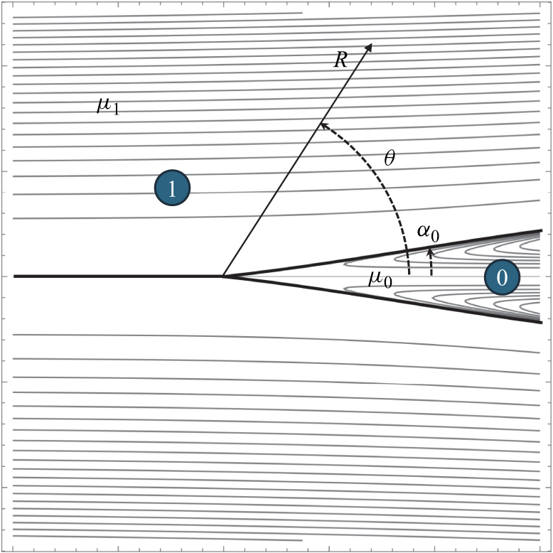


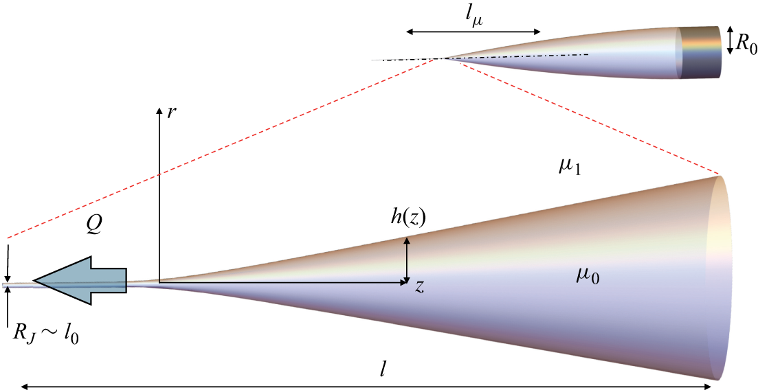


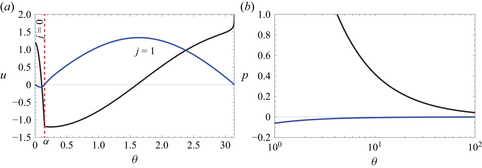


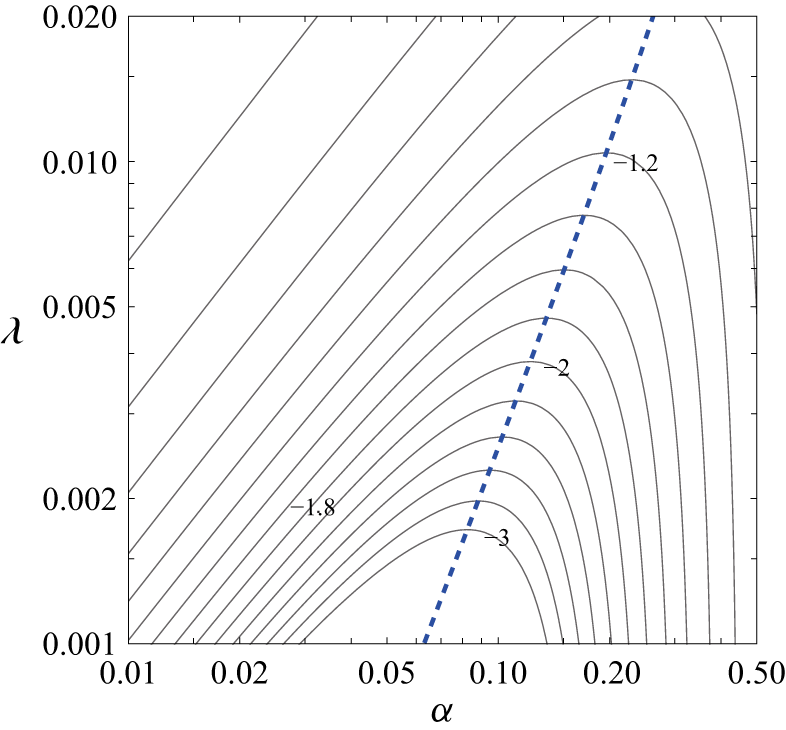


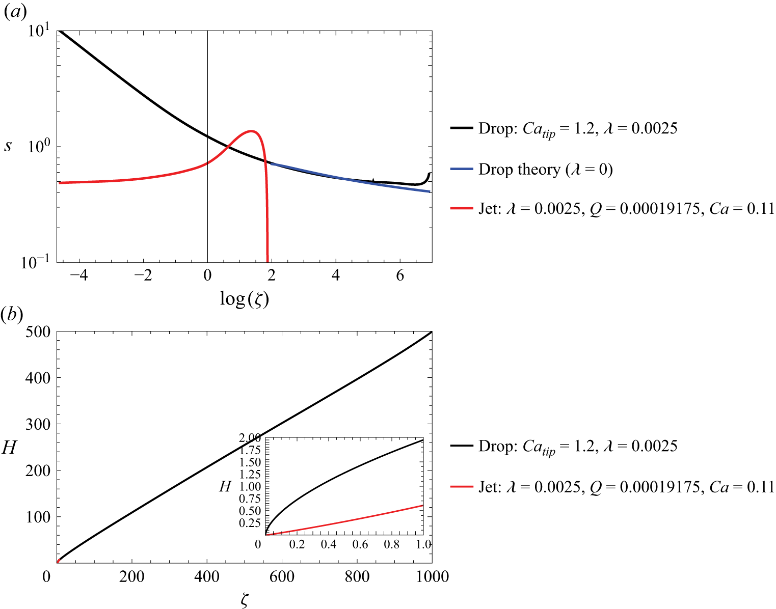


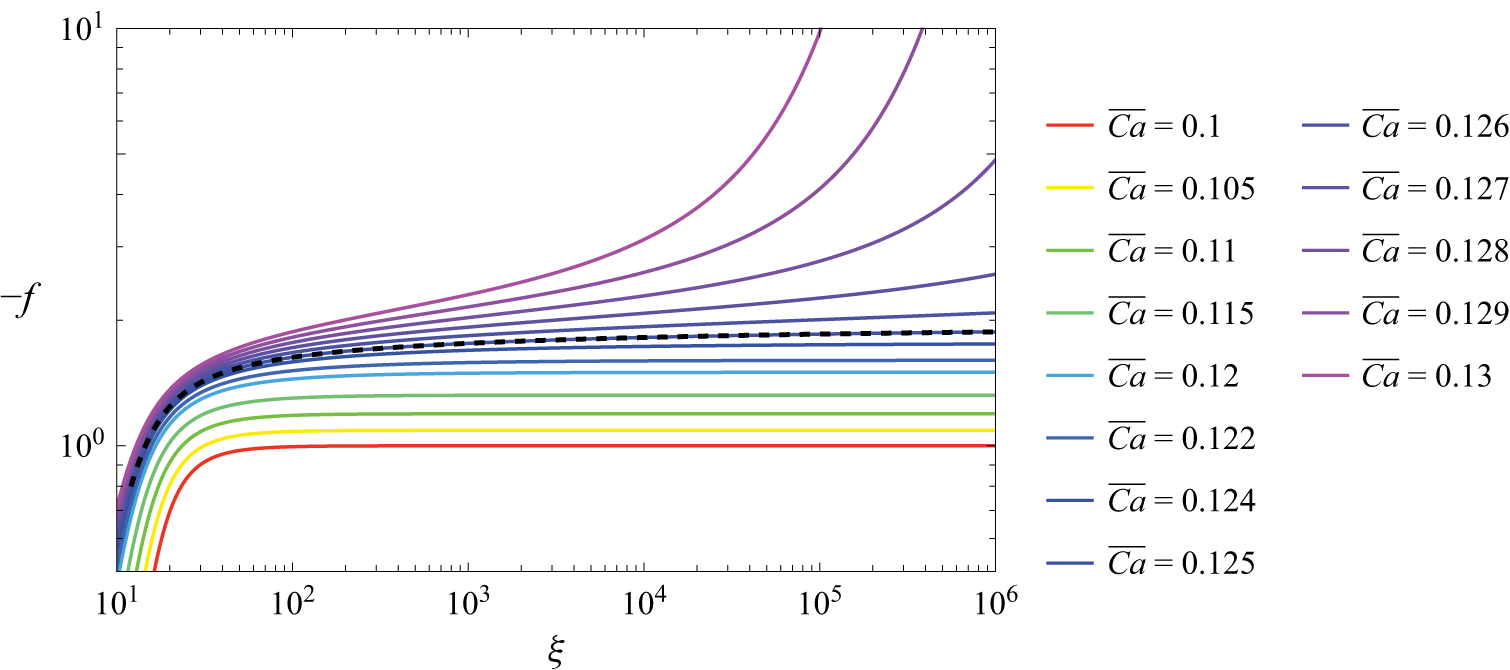


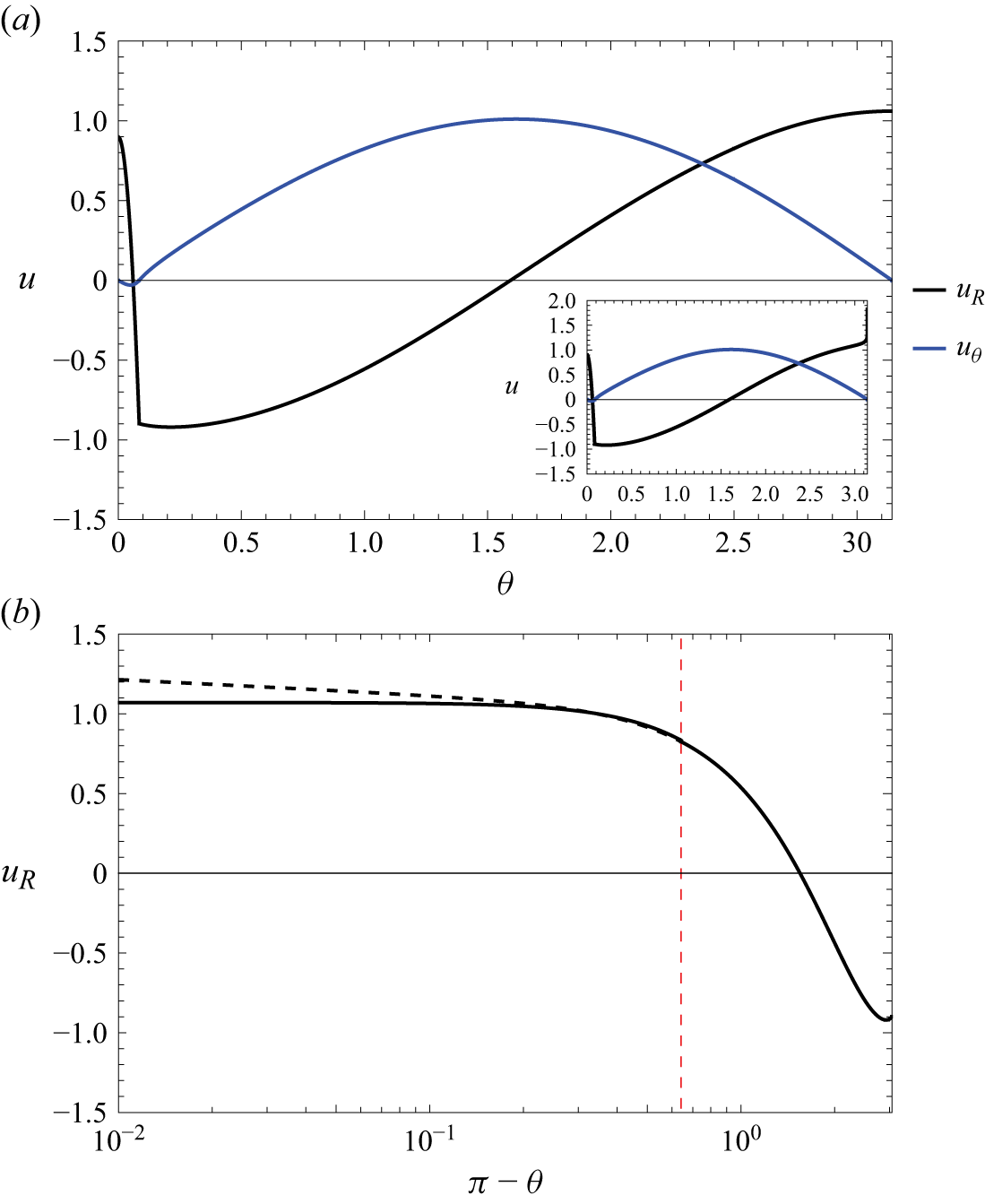


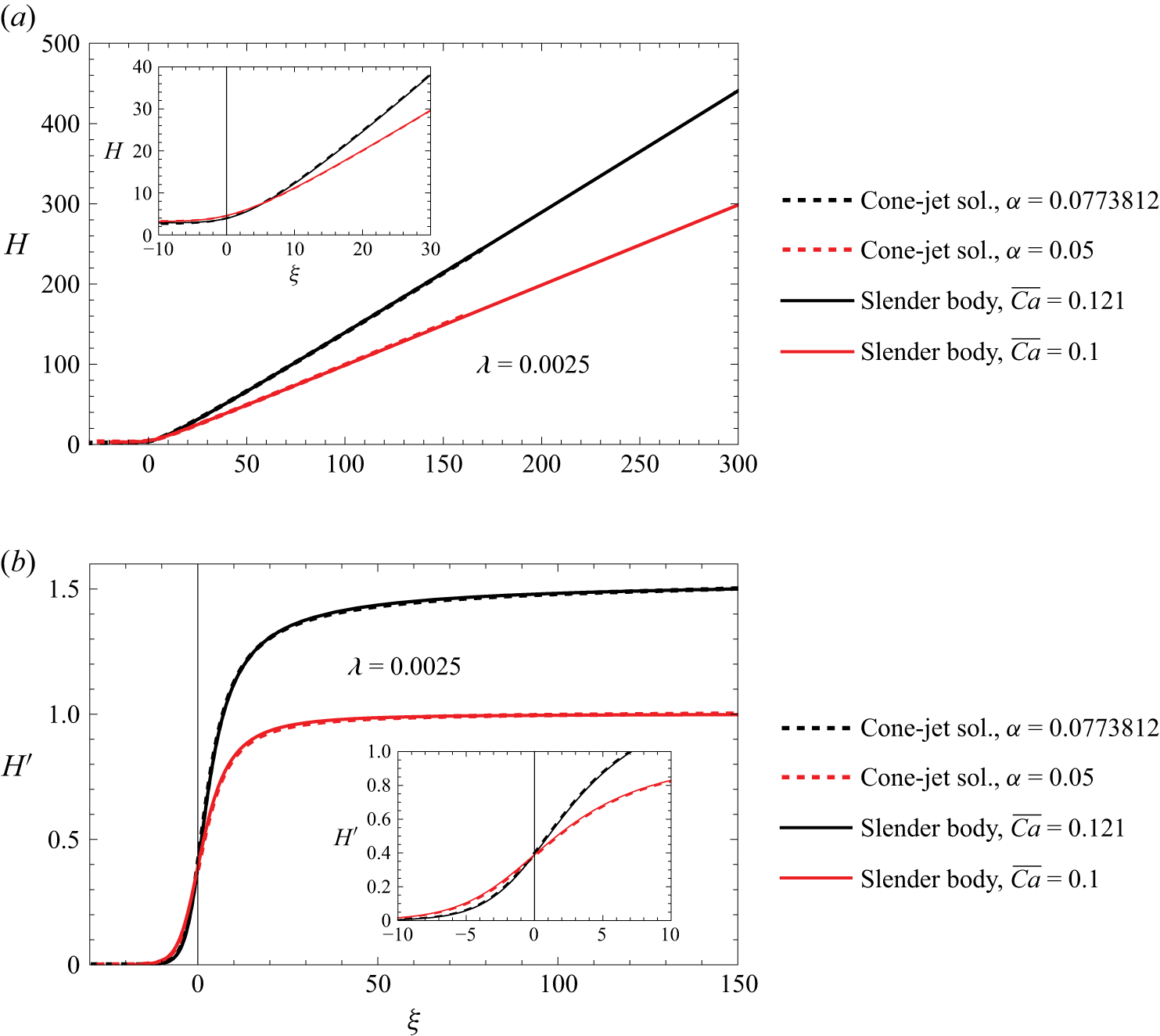


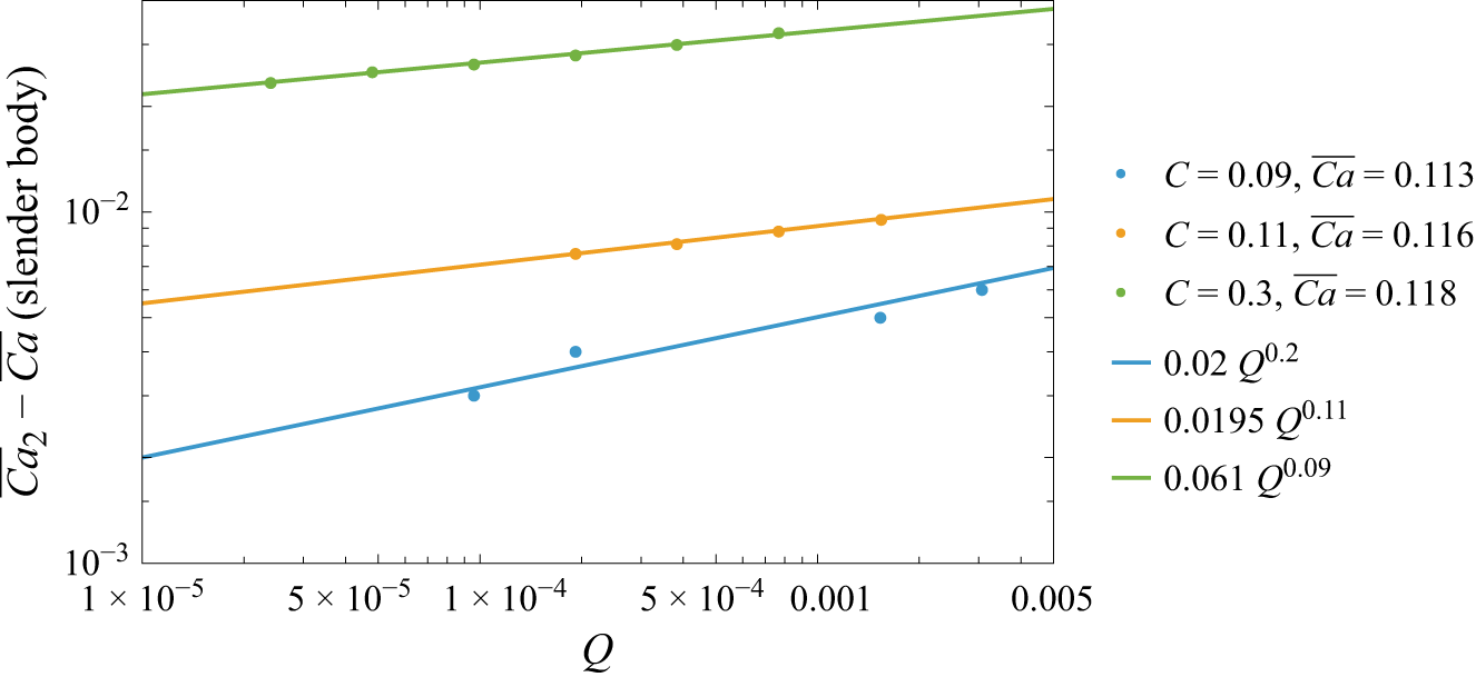


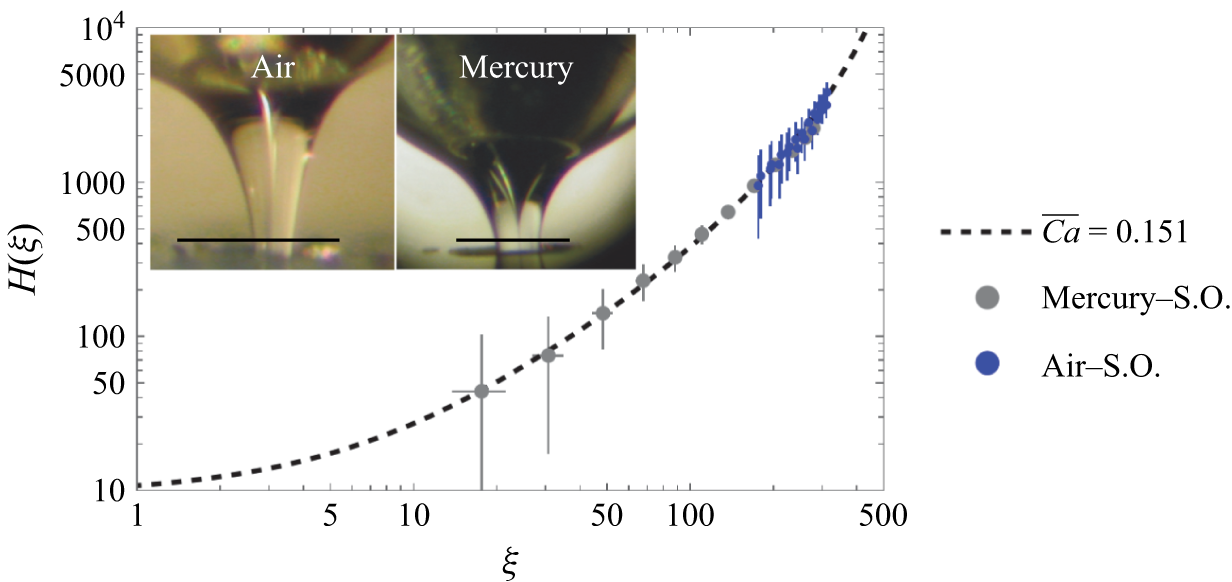


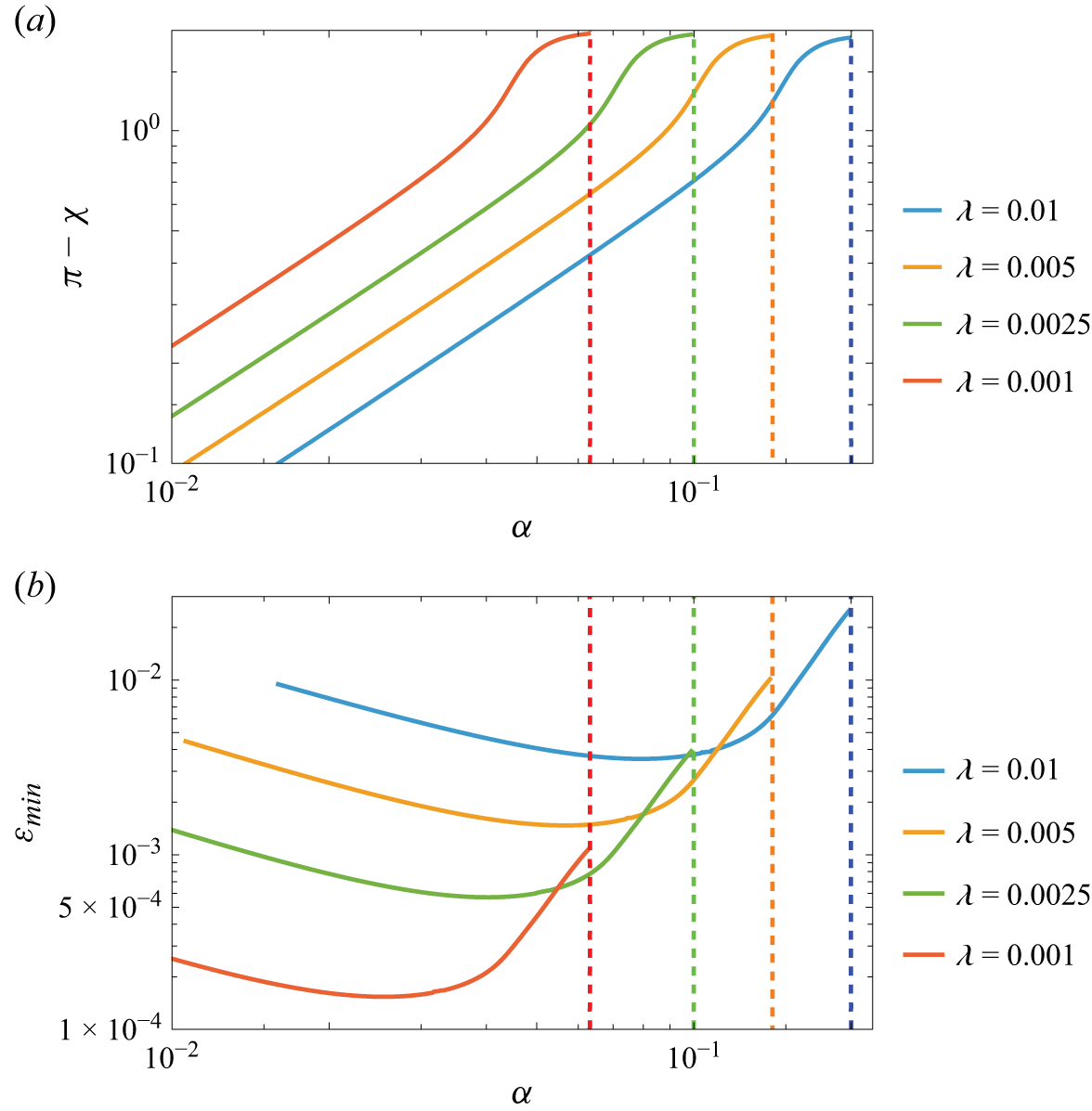


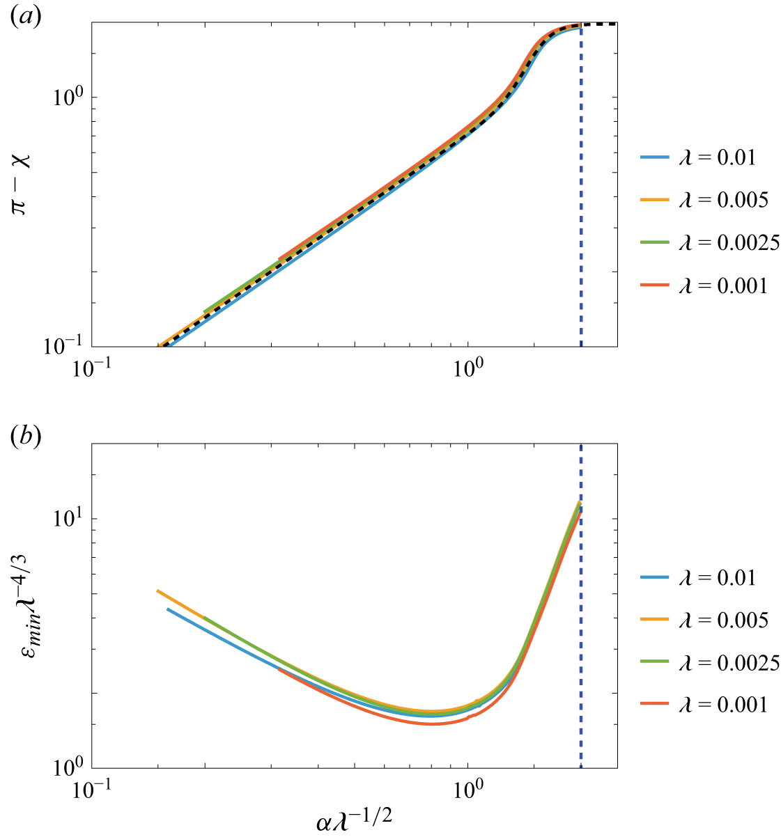


 Open access