



1. Introduction
In the classical Richardson–Kolmogorov view of the energy cascade, also known as the K41 theory (Kolmogorov Reference Kolmogorov1941a
,
Reference Kolmogorovb
,
Reference Kolmogorovc
), fully developed turbulent flows at sufficiently high Reynolds numbers consist of eddies covering a wide range of scales. The kinetic energy is transferred from larger to smaller scales. The K41 theory was derived based on the similarity framework, and is known for its simplicity and elegance. Based on the first and second similarity hypotheses, Kolmogorov (Reference Kolmogorov1941b
) derived the two-thirds law for the second-order longitudinal structure function (LSF) $\langle \delta u^{{\prime }2}\rangle (r)$
in the inertial range, that is,
$\langle \delta u^{{\prime }2}\rangle (r)$
in the inertial range, that is,
 \begin{align} \big\langle \delta u^{{\prime }2}\big\rangle (r)=C_2^{\textit{LSF}}{\varepsilon }^{2/3}r^{2/3}, \end{align}
where $\delta u^{{\prime }}(r) = u^{\prime }(\boldsymbol{x}+r\boldsymbol{e}_1)-u^{\prime }(\boldsymbol{x})$
represents the velocity increment between points
$\delta u^{{\prime }}(r) = u^{\prime }(\boldsymbol{x}+r\boldsymbol{e}_1)-u^{\prime }(\boldsymbol{x})$
represents the velocity increment between points $\boldsymbol{x}+r\boldsymbol{e}_1$
and
$\boldsymbol{x}+r\boldsymbol{e}_1$
and $\boldsymbol{x}$
. Here,
$\boldsymbol{x}$
. Here, $\boldsymbol{e}_1$
and
$\boldsymbol{e}_1$
and $r$
are the unit vector of the streamwise direction and the separation distance along the unit vector direction, respectively,
$r$
are the unit vector of the streamwise direction and the separation distance along the unit vector direction, respectively, $C_2^{\textit{LSF}}$
is a Kolmogorov (universal) constant for
$C_2^{\textit{LSF}}$
is a Kolmogorov (universal) constant for $\langle \delta u^{{\prime }2}\rangle (r)$
(Pope Reference Pope2000; Davidson Reference Davidson2004), and
$\langle \delta u^{{\prime }2}\rangle (r)$
(Pope Reference Pope2000; Davidson Reference Davidson2004), and $\varepsilon$
is the kinetic energy dissipation rate. In the same year, Kolmogorov (Reference Kolmogorov1941a
) also derived a simple expression for
$\varepsilon$
is the kinetic energy dissipation rate. In the same year, Kolmogorov (Reference Kolmogorov1941a
) also derived a simple expression for $\langle \delta u^{{\prime }3}\rangle (r)$
(hereafter referred to as the Kolmogorov
$\langle \delta u^{{\prime }3}\rangle (r)$
(hereafter referred to as the Kolmogorov $4/5$
law) from the transport equation of
$4/5$
law) from the transport equation of $\langle \delta u^{{\prime }2}\rangle (r)$
, expressed as
$\langle \delta u^{{\prime }2}\rangle (r)$
, expressed as $\langle \delta u^{{\prime }3}\rangle (r)=-4/5{\varepsilon r}$
. The Kolmogorov
$\langle \delta u^{{\prime }3}\rangle (r)=-4/5{\varepsilon r}$
. The Kolmogorov $4/5$
law reflects the mean rate and direction of energy transfer toward smaller scales at a scale
$4/5$
law reflects the mean rate and direction of energy transfer toward smaller scales at a scale $r$
within the inertial range. While this law is widely regarded as strictly valid for stationary isotropic turbulence at infinite Reynolds number, it has not yet been fully verified by experimental or direct numerical simulation (DNS) studies (Tang et al. Reference Tang, Antonia, Djenidi and Zhou2019).
$r$
within the inertial range. While this law is widely regarded as strictly valid for stationary isotropic turbulence at infinite Reynolds number, it has not yet been fully verified by experimental or direct numerical simulation (DNS) studies (Tang et al. Reference Tang, Antonia, Djenidi and Zhou2019).
Considering the large-scale fluctuations in energy dissipation, the shortcoming of the simplified K41 theory was predicted by Landau & Lifshits (Reference Landau and Lifshits1944) at an early stage, foreseeing the absence of a universal form for the structure of turbulence in the inertial range. A refined K62 theory (Kolmogorov Reference Kolmogorov1962) that abandons the concept of local universality has been proposed to account for the variation in $\varepsilon$
induced by large-scale motions. The K62 theory accounts for the deviations of the scaling exponents from the K41 predictions by taking small-scale intermittency into consideration. Extensive studies (both experimental (Stolovitzky, Kailasnath & Sreenivasan Reference Stolovitzky, Kailasnath and Sreenivasan1992; Stolovitzky & Sreenivasan Reference Stolovitzky and Sreenivasan1994; Lawson et al. Reference Lawson, Bodenschatz, Knutsen, Dawson and Worth2019) and numerical (Wang et al. Reference Wang, Chen, Brasseur and Wyngaard1996; Schumacher, Sreenivasan & Yakhot Reference Schumacher, Sreenivasan and Yakhot2007; Yao et al. Reference Yao, Yeung, Zaki and Meneveau2024)) have been performed and provided evidence supporting the K62 theory in fully turbulent flows, particularly based on results from the atmospheric surface layer (Obukhov Reference Obukhov1962). However, recent studies have suggested that there is no reason to abandon K41 (Sreenivasan & Dhruva Reference Sreenivasan and Dhruva1998; Antonia & Burattini Reference Antonia and Burattini2006; Antonia et al. Reference Antonia, Djenidi, Danaila and Tang2017; Tang et al. Reference Tang, Antonia, Djenidi, Danaila and Zhou2017, Reference Tang, Antonia, Djenidi and Zhou2019; Antonia et al. Reference Antonia, Tang, Danaila, Djenidi and Zhou2019a
,
Reference Antonia, Tang, Djenidi and Zhoub
). One reason is that both the K41 and K62 theories rely on the assumption of an infinite Reynolds number. However, experimental evidence supporting anomalous scaling of the structure function (Sreenivasan & Antonia Reference Sreenivasan and Antonia1997) has not fully accounted for finite-Reynolds-number (FRN) effects. Ishihara et al. (Reference Ishihara, Gotoh and Kaneda2009, Reference Ishihara, Morishita, Yokokawa, Uno and Kaneda2016) investigated the three-dimensional energy spectrum of stationary forced periodic box turbulence over a wide range of
$\varepsilon$
induced by large-scale motions. The K62 theory accounts for the deviations of the scaling exponents from the K41 predictions by taking small-scale intermittency into consideration. Extensive studies (both experimental (Stolovitzky, Kailasnath & Sreenivasan Reference Stolovitzky, Kailasnath and Sreenivasan1992; Stolovitzky & Sreenivasan Reference Stolovitzky and Sreenivasan1994; Lawson et al. Reference Lawson, Bodenschatz, Knutsen, Dawson and Worth2019) and numerical (Wang et al. Reference Wang, Chen, Brasseur and Wyngaard1996; Schumacher, Sreenivasan & Yakhot Reference Schumacher, Sreenivasan and Yakhot2007; Yao et al. Reference Yao, Yeung, Zaki and Meneveau2024)) have been performed and provided evidence supporting the K62 theory in fully turbulent flows, particularly based on results from the atmospheric surface layer (Obukhov Reference Obukhov1962). However, recent studies have suggested that there is no reason to abandon K41 (Sreenivasan & Dhruva Reference Sreenivasan and Dhruva1998; Antonia & Burattini Reference Antonia and Burattini2006; Antonia et al. Reference Antonia, Djenidi, Danaila and Tang2017; Tang et al. Reference Tang, Antonia, Djenidi, Danaila and Zhou2017, Reference Tang, Antonia, Djenidi and Zhou2019; Antonia et al. Reference Antonia, Tang, Danaila, Djenidi and Zhou2019a
,
Reference Antonia, Tang, Djenidi and Zhoub
). One reason is that both the K41 and K62 theories rely on the assumption of an infinite Reynolds number. However, experimental evidence supporting anomalous scaling of the structure function (Sreenivasan & Antonia Reference Sreenivasan and Antonia1997) has not fully accounted for finite-Reynolds-number (FRN) effects. Ishihara et al. (Reference Ishihara, Gotoh and Kaneda2009, Reference Ishihara, Morishita, Yokokawa, Uno and Kaneda2016) investigated the three-dimensional energy spectrum of stationary forced periodic box turbulence over a wide range of $ \textit{Re}_\lambda$
(=167–2297) and found that the spectrum exhibits clear FRN effects. Furthermore, significant FRN effects have also been observed in other turbulence statistics, such as structure functions (Tang et al. Reference Tang, Antonia, Djenidi, Danaila and Zhou2017; Antonia et al. Reference Antonia, Tang, Danaila, Djenidi and Zhou2019a
; Tang et al. Reference Tang, Antonia and Djenidi2023) and pressure spectra (Tsuji & Ishihara Reference Tsuji and Ishihara2003). One interesting finding is that these statistical results appear to increasingly approach the K41 asymptotes as the Reynolds number increases.
$ \textit{Re}_\lambda$
(=167–2297) and found that the spectrum exhibits clear FRN effects. Furthermore, significant FRN effects have also been observed in other turbulence statistics, such as structure functions (Tang et al. Reference Tang, Antonia, Djenidi, Danaila and Zhou2017; Antonia et al. Reference Antonia, Tang, Danaila, Djenidi and Zhou2019a
; Tang et al. Reference Tang, Antonia and Djenidi2023) and pressure spectra (Tsuji & Ishihara Reference Tsuji and Ishihara2003). One interesting finding is that these statistical results appear to increasingly approach the K41 asymptotes as the Reynolds number increases.
In both nature and engineering, a common flow phenomenon is the turbulent flow region, separated from the non-turbulent flow region by a thin shear layer called the turbulent/non-turbulent interface (TNTI) (da Silva et al. Reference da Silva, Hunt, Eames and Westerweel2014). The separation between turbulent and non-turbulent regions indicates large-scale fluctuations in energy production and dissipation, and leads to characteristic features of external intermittency near the turbulent boundary (LaRue & Libby Reference LaRue and Libby1976; Sreenivasan Reference Sreenivasan1991). A comprehensive understanding of external intermittency is crucial for modelling the mixing transition problem (Wang & Fu Reference Wang and Fu2011; Xie et al. Reference Xie, Qi, Xiao, Zhang and Zhao2025a
) in practical engineering applications. However, until now, investigations of FRN effects on structure functions have focused on the fully turbulent region, while the influence of external intermittency has been significantly overlooked. One remaining important question is whether the conditional second-order structure function in the intermittent region follows the classical $2/3$
scaling law, while the conditional third-order structure function satisfies the Kolmogorov
$2/3$
scaling law, while the conditional third-order structure function satisfies the Kolmogorov $4/5$
law. This paper focuses on FRN effects on structure functions in the intermittent region due to the presence of the TNTI.
$4/5$
law. This paper focuses on FRN effects on structure functions in the intermittent region due to the presence of the TNTI.
Davidson (Reference Davidson2004) and Monin & Yaglom (Reference Monin and Yaglom2007) proposed a simple two-state model (strong dissipation and weak dissipation states) based on K41 theory to explain the effect of large-scale inhomogeneities on small-scale universality. Despite lacking a solid theoretical foundation, this model has also been used to roughly predict the Kolmogorov constant with large-scale energy injection (Chien, Blum & Voth Reference Chien, Blum and Voth2013). However, a recent study by Watanabe et al. (Reference Watanabe, Silva and Nagata2019a
) suggested that non-equilibrium dissipation occurs near the TNTI at relatively low Reynolds numbers, where Taylor’s dissipation law does not apply. Turbulence near the TNTI layer exhibits pronounced large-scale inhomogeneity and anisotropy at relatively low Reynolds numbers (da Silva et al. Reference da Silva, Hunt, Eames and Westerweel2014; Zecchetto & da Silva Reference Zecchetto and da Silva2021). This suggests that the direct application of this model to the intermittent region may be limited, as turbulence in this region may exist in two different states. In contrast, turbulence near the TNTI layer becomes more isotropic at higher Reynolds numbers, as demonstrated by the analysis of the anisotropy tensors of Reynolds stress and vorticity (Zhang, Watanabe & Nagata Reference Zhang, Watanabe and Nagata2023). Therefore, the two-state model also needs to take into account Reynolds number dependence when applied to the intermittent region. This is necessary to explain the variation of the Kolmogorov constant with the intermittency factor $\gamma$
.
$\gamma$
.
The influence of large-scale motions on the small scales causes the second-order structure function to change from flow to flow (Blum et al. Reference Blum, Bewley, Bodenschatz, Gibert, Gylfason, Mydlarski, Voth, Xu and Yeung2011). Recently, it has been demonstrated that an extended $2/3$
power law holds for the second-order structure function in the developing region of various grid-generated turbulence (e.g. regular grid, fractal-square grid, singe-square grid), clearly violating the well-known K41 theory (Laizet, Vassilicos & Cambon Reference Laizet, Vassilicos and Cambon2013; Zhou et al. Reference Zhou, Nagata, Sakai, Ito and Hayase2016; Alves Portela, Papadakis & Vassilicos Reference Alves Portela, Papadakis and Vassilicos2017). Alves Portela et al. (Reference Alves Portela, Papadakis and Vassilicos2017) and Zhou et al. (Reference Zhou, Nagata, Sakai and Watanabe2019, Reference Zhou, Nagata, Sakai, Watanabe, Ito and Hayase2020) pointed out that the energy spectrum exhibits the classical approximate −
$2/3$
power law holds for the second-order structure function in the developing region of various grid-generated turbulence (e.g. regular grid, fractal-square grid, singe-square grid), clearly violating the well-known K41 theory (Laizet, Vassilicos & Cambon Reference Laizet, Vassilicos and Cambon2013; Zhou et al. Reference Zhou, Nagata, Sakai, Ito and Hayase2016; Alves Portela, Papadakis & Vassilicos Reference Alves Portela, Papadakis and Vassilicos2017). Alves Portela et al. (Reference Alves Portela, Papadakis and Vassilicos2017) and Zhou et al. (Reference Zhou, Nagata, Sakai and Watanabe2019, Reference Zhou, Nagata, Sakai, Watanabe, Ito and Hayase2020) pointed out that the energy spectrum exhibits the classical approximate − $5/3$
scaling law in the intermittency region associated with large-scale vortex shedding. The key to explaining the appearance of the −
$5/3$
scaling law in the intermittency region associated with large-scale vortex shedding. The key to explaining the appearance of the − $5/3$
spectrum lies in the phenomenological model that within the intermittent flow region, the turbulent components in the dissipation and intermediate ranges exhibit similarity properties akin to those in fully turbulent flows (Zhou et al. Reference Zhou, Nagata, Ito, Sakai and Hayase2023). Zhou et al. (Reference Zhou, Nagata, Ito, Sakai and Hayase2023) further indicate that the universal constant
$5/3$
spectrum lies in the phenomenological model that within the intermittent flow region, the turbulent components in the dissipation and intermediate ranges exhibit similarity properties akin to those in fully turbulent flows (Zhou et al. Reference Zhou, Nagata, Ito, Sakai and Hayase2023). Zhou et al. (Reference Zhou, Nagata, Ito, Sakai and Hayase2023) further indicate that the universal constant $C_{k1}$
in spectral space exhibits a clear power-law dependence on the intermittency factor
$C_{k1}$
in spectral space exhibits a clear power-law dependence on the intermittency factor $\gamma$
, i.e.
$\gamma$
, i.e. $C_{k1}\sim \gamma ^{1/3}$
. A parallel study was recently carried out in the intermittent region to examine the emergence of the
$C_{k1}\sim \gamma ^{1/3}$
. A parallel study was recently carried out in the intermittent region to examine the emergence of the $2/3$
scaling law in the inertial range of the structure function (Xie et al. Reference Xie, Xiong, Zheng, Nagata, Watanabe and Zhou2025b
). The results indicate that the universal constant
$2/3$
scaling law in the inertial range of the structure function (Xie et al. Reference Xie, Xiong, Zheng, Nagata, Watanabe and Zhou2025b
). The results indicate that the universal constant $C_{2}^{\textit{LSF}}$
in physical space exhibits the same dependence on
$C_{2}^{\textit{LSF}}$
in physical space exhibits the same dependence on $\gamma$
, i.e.
$\gamma$
, i.e. $C_{2}^{\textit{LSF}}\sim \gamma ^{1/3}$
. However, the existence of the TNTI induces blocking/sheltering mechanism (Hunt & Durbin Reference Hunt and Durbin1999; da Silva et al. Reference da Silva, Hunt, Eames and Westerweel2014), causing the structure function to exhibit unique behaviour near TNTI (Xie et al. Reference Xie, Xiong, Zheng, Nagata, Watanabe and Zhou2025b
). Compared with second-order structure functions, higher-order structure functions are highly sensitive to the effect of external intermittency (Gauding et al. Reference Gauding, Bode, Brahami, Varea and Danaila2021). Another pertinent question concerns the self-similarity of higher-order structure functions in the intermittent region, as well as the effect of the TNTI blocking/sheltering mechanism on their self-similar behaviour.
$C_{2}^{\textit{LSF}}\sim \gamma ^{1/3}$
. However, the existence of the TNTI induces blocking/sheltering mechanism (Hunt & Durbin Reference Hunt and Durbin1999; da Silva et al. Reference da Silva, Hunt, Eames and Westerweel2014), causing the structure function to exhibit unique behaviour near TNTI (Xie et al. Reference Xie, Xiong, Zheng, Nagata, Watanabe and Zhou2025b
). Compared with second-order structure functions, higher-order structure functions are highly sensitive to the effect of external intermittency (Gauding et al. Reference Gauding, Bode, Brahami, Varea and Danaila2021). Another pertinent question concerns the self-similarity of higher-order structure functions in the intermittent region, as well as the effect of the TNTI blocking/sheltering mechanism on their self-similar behaviour.
The objective of this study is to investigate the aforementioned questions within the framework of a temporally evolving turbulent plane jet. In particular, we focus on the FRN effect of the second- and third-order structure functions in the intermittent region. Note that the different flow types (e.g. the temporally evolving jet, the spatially evolving jet and spatially evolving round jet) are expected to lead to distinctly different growth behaviour (van Reeuwijk, Vassilicos & Craske Reference van Reeuwijk, Vassilicos and Craske2021; Er, Laval & Vassilicos Reference Er, Laval and Vassilicos2023). More specifically, the temporally developing self-similar turbulent jet conserves volume flux. In contrast, the spatially developing jet conserves momentum flux. This means that applying similar analytical methods in this paper to spatially evolving jets (e.g. the spatially evolving round jet), which are of more practical interest, requires careful consideration. The remainder of the paper is organised as follows. In § 2, we provide a concise overview of the numerical methods and parameters employed for simulating the temporally evolving turbulent plane jet. A simplified two-state model based on K41 theory is used to investigate the self-similarity of the structure functions, as discussed in § 3. In § 4, the self-similarity of the third-order structure function and the contribution of the unsteady term are further examined. The FRN effect on the structure functions in the intermittent and fully turbulent regions is discussed in § 5. In § 6, we highlight the main findings and propose potential avenues for future research.
2. Numerical details and turbulence characteristics of the turbulent plane jet
2.1. Numerical details and computational parameters
In this study, the three-dimensional data from prior DNS studies of the temporally evolving turbulent jet performed by Watanabe et al. (Reference Watanabe, Zhang and Nagata2019b
) and Hayashi et al. (Reference Hayashi, Watanabe and Nagata2021) are used to investigate the effects of external intermittency on the second- and third-order structure functions. In the streamwise $X$
and spanwise
$X$
and spanwise $Z$
directions, periodic boundary conditions are imposed and uniformly distributed spacings are used. In the normal
$Z$
directions, periodic boundary conditions are imposed and uniformly distributed spacings are used. In the normal $Y$
direction, a free-slip boundary condition is applied and the grid is stretched using a mapping function (Watanabe et al. Reference Watanabe, Zhang and Nagata2019b
). The spatial derivatives are discretised using the fully conservative central difference scheme proposed by Morinishi et al. (Reference Morinishi, Lund, Vasilyev and Moin1998). A second-order scheme is applied in the normal
$Y$
direction, a free-slip boundary condition is applied and the grid is stretched using a mapping function (Watanabe et al. Reference Watanabe, Zhang and Nagata2019b
). The spatial derivatives are discretised using the fully conservative central difference scheme proposed by Morinishi et al. (Reference Morinishi, Lund, Vasilyev and Moin1998). A second-order scheme is applied in the normal $Y$
direction, while fourth-order difference schemes are applied in the streamwise
$Y$
direction, while fourth-order difference schemes are applied in the streamwise $X$
and spanwise
$X$
and spanwise $Z$
directions. A third-order Runge–Kutta method is employed for the time advancement and the Bi-CGSTAB method is adopted to solve the pressure Poisson equation. Nagarajan, Lele & Ferziger (Reference Nagarajan, Lele and Ferziger2003) and Suzuki et al. (Reference Suzuki, Nagata, Sakai, Hayase, Hasegawa and Ushijima2013) quantified the errors in the first- and second-order derivatives, and higher-order statistics of the fourth-order and second-order fully conservative finite difference schemes using Fourier analysis. The results indicate that each term in the Reynolds-stress transport equation shows good agreement with the corresponding results obtained using spectral methods. For a more detailed examination of the errors associated with the finite difference schemes adopted, please refer to Appendix A of Watanabe et al. (Reference Watanabe, Riley, Nagata, Onishi and Matsuda2018a
).
$Z$
directions. A third-order Runge–Kutta method is employed for the time advancement and the Bi-CGSTAB method is adopted to solve the pressure Poisson equation. Nagarajan, Lele & Ferziger (Reference Nagarajan, Lele and Ferziger2003) and Suzuki et al. (Reference Suzuki, Nagata, Sakai, Hayase, Hasegawa and Ushijima2013) quantified the errors in the first- and second-order derivatives, and higher-order statistics of the fourth-order and second-order fully conservative finite difference schemes using Fourier analysis. The results indicate that each term in the Reynolds-stress transport equation shows good agreement with the corresponding results obtained using spectral methods. For a more detailed examination of the errors associated with the finite difference schemes adopted, please refer to Appendix A of Watanabe et al. (Reference Watanabe, Riley, Nagata, Onishi and Matsuda2018a
).
Numerical parameters for the DNS of temporally evolving turbulent plane jets. The turbulence statistics at $T/T_{\textit{ref}}=20.0$
, including
$T/T_{\textit{ref}}=20.0$
, including $\Delta X/\eta$
,
$\Delta X/\eta$
, $\Delta Y/\eta$
,
$\Delta Y/\eta$
, $\Delta Z/\eta$
and
$\Delta Z/\eta$
and $ \textit{Re}_\lambda$
, are computed at the centre plane of the jet.
$ \textit{Re}_\lambda$
, are computed at the centre plane of the jet.

Table 1. Long description
The table presents numerical parameters for the direct numerical simulation (DNS) of temporally evolving turbulent plane jets. It includes columns for Reynolds number (ReH), number of samples (Ns), initial momentum thickness to half-velocity thickness ratio (θ0/H), and various grid dimensions and spacings. The table has two rows of data, each representing different simulation conditions. The first row shows ReH of
 , Ns of 6, θ0/H of 1/100, and grid dimensions LX/H of 6, LY/H of 10, and LZ/H of 4, with corresponding grid points NX of 864, NY of 1200, and NZ of 576. The spacings ΔX/η, ΔY/η, and ΔZ/η are 1.5, 1.2, and 1.5 respectively, with a final Reynolds number Reλ of 100. The second row shows ReH of
 , Ns of 1, θ0/H of 1/100, and grid dimensions LX/H of 6, LY/H of 10, and LZ/H of 4, with corresponding grid points NX of 4608, NY of 5800, and NZ of 3072. The spacings ΔX/η, ΔY/η, and ΔZ/η are 1.7, 1.5, and 1.7 respectively, with a final Reynolds number Reλ of 353. The turbulence statistics at x=6H, including u, v, and w, are computed at the center plane of the jet.
The initial streamwise velocity component of a turbulent jet is given by the hyperbolic tangent function (da Silva & Pereira Reference da Silva and Pereira2008; Hayashi, Watanabe & KNagata Reference Hayashi, Watanabe and Nagata2021), while the normal and spanwise velocity components are set to zero. Considering that the Reynolds number significantly affects the behaviour of structure functions (Pearson & Antonia Reference Pearson and Antonia2001), the present study uses two different cases to investigate the effects of external intermittency on the longitudinal and transverse structure functions. Although high-fidelity and high-resolution three-dimensional DNS data are obtained using state-of-the-art massively parallel computations, the Reynolds number remains limited. Therefore, the influence of small-scale intermittency and the related anomalous scaling is not considered in the present study. The global Reynolds number based on the initial streamwise velocity $U_{\textit{in}}$
along the centreline and the jet width
$U_{\textit{in}}$
along the centreline and the jet width $H$
is defined as
$H$
is defined as $ \textit{Re}_H=U_{\textit{in}} H / \nu$
, and takes the values
$ \textit{Re}_H=U_{\textit{in}} H / \nu$
, and takes the values $10^4$
and
$10^4$
and $10^5$
. The corresponding mesh numbers are
$10^5$
. The corresponding mesh numbers are $N_X \times N_Y \times N_Z = 864 \times 1200 \times 576$
and
$N_X \times N_Y \times N_Z = 864 \times 1200 \times 576$
and $N_X \times N_Y \times N_Z = 4608 \times 5800 \times 3072$
, respectively. The numerical parameters of DNS are summarised in table 1 and a schematic of the DNS of the turbulent plane jet is shown in figure 1. It is well known that the computational cost of temporally evolving flows is significantly lower than that of spatially evolving flows at the same Reynolds number. In other words, temporally evolving flows often provide a more feasible approach for accessing data at higher Reynolds numbers. Furthermore, for the temporally evolving jet, the ensemble averages are taken over the two homogeneous directions (i.e. the streamwise and spanwise directions), which enables the statistical results to converge readily. Another motivation for selecting the jet configuration arises from our previous studies showing that the second-order structure function in the developing region of spatially evolving wakes is significantly affected by large-scale strong vortex shedding. The observed power-law exponent is
$N_X \times N_Y \times N_Z = 4608 \times 5800 \times 3072$
, respectively. The numerical parameters of DNS are summarised in table 1 and a schematic of the DNS of the turbulent plane jet is shown in figure 1. It is well known that the computational cost of temporally evolving flows is significantly lower than that of spatially evolving flows at the same Reynolds number. In other words, temporally evolving flows often provide a more feasible approach for accessing data at higher Reynolds numbers. Furthermore, for the temporally evolving jet, the ensemble averages are taken over the two homogeneous directions (i.e. the streamwise and spanwise directions), which enables the statistical results to converge readily. Another motivation for selecting the jet configuration arises from our previous studies showing that the second-order structure function in the developing region of spatially evolving wakes is significantly affected by large-scale strong vortex shedding. The observed power-law exponent is $1$
, which is significantly larger than the classical value of
$1$
, which is significantly larger than the classical value of $2/3$
. Therefore, it is a reasonable choice to use a temporally evolving plane jet for this investigation. However, a significant limitation of temporally evolving flows is the limited number of spatial samples available in a single instantaneous field. This makes it difficult to obtain statistically converged results, particularly for higher-order statistics such as the third-order structure function. For this reason, the DNS is performed
$2/3$
. Therefore, it is a reasonable choice to use a temporally evolving plane jet for this investigation. However, a significant limitation of temporally evolving flows is the limited number of spatial samples available in a single instantaneous field. This makes it difficult to obtain statistically converged results, particularly for higher-order statistics such as the third-order structure function. For this reason, the DNS is performed $N_S$
times for each Reynolds number
$N_S$
times for each Reynolds number $ \textit{Re}_H$
using different initial velocity perturbations, where the values of
$ \textit{Re}_H$
using different initial velocity perturbations, where the values of $N_S$
are listed in table 1. Note that the strength of the random initial perturbations is consistent and the root mean square (r.m.s.) magnitude of the perturbations is equal to
$N_S$
are listed in table 1. Note that the strength of the random initial perturbations is consistent and the root mean square (r.m.s.) magnitude of the perturbations is equal to $2.5\,\%$
of the initial mean streamwise velocity at the centre plane. The mean streamwise velocity and the r.m.s. velocity components in all three directions were examined, which showed reasonably good agreement with previous numerical simulations and experimental data. For further description of the numerical validation, one can refer to Watanabe et al. (Reference Watanabe, Zhang and Nagata2019b
) and Hayashi et al. (Reference Hayashi, Watanabe and Nagata2021).
$2.5\,\%$
of the initial mean streamwise velocity at the centre plane. The mean streamwise velocity and the r.m.s. velocity components in all three directions were examined, which showed reasonably good agreement with previous numerical simulations and experimental data. For further description of the numerical validation, one can refer to Watanabe et al. (Reference Watanabe, Zhang and Nagata2019b
) and Hayashi et al. (Reference Hayashi, Watanabe and Nagata2021).
Since the thickness of the TNTI is comparable to the Kolmogorov scale (Watanabe et al. Reference Watanabe, Zhang and Nagata2018b
; Zhang, Watanabe & Nagata Reference Zhang, Watanabe and Nagata2018), high spatial resolution is required for accurate numerical studies of external intermittency. In the centre plane of the jet, the normalised spatial resolutions in the $X$
and
$X$
and $Y$
directions are
$Y$
directions are $ \mathrm{\Delta } X/\eta = 1.5,\, \Delta Y/\eta = 1.2$
for
$ \mathrm{\Delta } X/\eta = 1.5,\, \Delta Y/\eta = 1.2$
for $ Re_H = 10^4$
and
$ Re_H = 10^4$
and $ \Delta X/\eta = 1.7,\, \Delta Y/\eta = 1.5$
for
$ \Delta X/\eta = 1.7,\, \Delta Y/\eta = 1.5$
for $ Re_H = 10^5$
at
$ Re_H = 10^5$
at $T/T_{\textit{ref}}=20.0$
, where
$T/T_{\textit{ref}}=20.0$
, where $\eta =(\nu ^{3}/\varepsilon )^{1/4}$
represents the Kolmogorov length scale and
$\eta =(\nu ^{3}/\varepsilon )^{1/4}$
represents the Kolmogorov length scale and $\varepsilon =2\nu \langle s_{\textit{ij}}s_{\textit{ij}}\rangle$
is the kinetic energy dissipation rate. Note that the normalised spatial resolutions in the
$\varepsilon =2\nu \langle s_{\textit{ij}}s_{\textit{ij}}\rangle$
is the kinetic energy dissipation rate. Note that the normalised spatial resolutions in the $X$
and
$X$
and $Z$
directions are identical, i.e.
$Z$
directions are identical, i.e. $\Delta X/\eta = \Delta Z/\eta$
. The local Reynolds numbers,
$\Delta X/\eta = \Delta Z/\eta$
. The local Reynolds numbers, $ Re_\lambda$
, is calculated using the Taylor microscale
$ Re_\lambda$
, is calculated using the Taylor microscale $ \lambda = u_{\textit{rms}} / \sqrt {\langle (\partial u^{\prime }/\partial x)^{2}\rangle }$
and the r.m.s. velocity
$ \lambda = u_{\textit{rms}} / \sqrt {\langle (\partial u^{\prime }/\partial x)^{2}\rangle }$
and the r.m.s. velocity $ u_{\textit{rms}}$
of the streamwise component along the centre plane of the jet. For
$ u_{\textit{rms}}$
of the streamwise component along the centre plane of the jet. For $ \textit{Re}_H = 10^4$
and
$ \textit{Re}_H = 10^4$
and $10^5$
, these values remain approximately constant after reaching the fully developed state at
$10^5$
, these values remain approximately constant after reaching the fully developed state at $100$
and
$100$
and $353$
, respectively. Here, the angled brackets
$353$
, respectively. Here, the angled brackets $\langle \rangle$
denote the ensemble average of statistical quantities over the
$\langle \rangle$
denote the ensemble average of statistical quantities over the $X$
–
$X$
– $Z$
plane, taking into account the flow symmetry in the
$Z$
plane, taking into account the flow symmetry in the $Y$
direction. The spatial resolution and turbulent Reynolds number are also presented in table 1.
$Y$
direction. The spatial resolution and turbulent Reynolds number are also presented in table 1.
2.2. Large-scale and small-scale intermittency of the turbulent plane jet
Schematic of the DNS of a turbulent plane jet. (a) Two-dimensional initial velocity field in the $X$
–
$X$
– $Y$
plane; (b) three-dimensional computational domain together with a randomly chosen vorticity field in the
$Y$
plane; (b) three-dimensional computational domain together with a randomly chosen vorticity field in the $X$
–
$X$
– $Y$
plane. The initial jet parameters are also shown, where
$Y$
plane. The initial jet parameters are also shown, where $H$
denotes the initial jet width and
$H$
denotes the initial jet width and $U_{\textit{in}}$
denotes the initial centreline velocity of the jet.
$U_{\textit{in}}$
denotes the initial centreline velocity of the jet.

Figure 1. Long description
A schematic of the DNS of a turbulent plane jet. The left part shows a two-dimensional initial velocity field in the plane, with labels indicating the initial jet width and the initial centerline velocity of the jet. The right part displays a three-dimensional computational domain with a randomly chosen vorticity field in the plane. The jet flow is indicated with arrows, and the ambient flow is also labeled.
Logarithmic contours of the vorticity magnitude $|\boldsymbol{\omega }|$
at the cross-wise position
$|\boldsymbol{\omega }|$
at the cross-wise position $Y/b_U = 1.6$
. The solid white line indicates the outer edge of the TNTI, which is defined by the vorticity threshold
$Y/b_U = 1.6$
. The solid white line indicates the outer edge of the TNTI, which is defined by the vorticity threshold $\omega _{{th}} = 0.01 \langle |\boldsymbol{\omega }|\rangle _{C}$
. (a)
$\omega _{{th}} = 0.01 \langle |\boldsymbol{\omega }|\rangle _{C}$
. (a) $ \textit{Re}_H=10^4$
; (b)
$ \textit{Re}_H=10^4$
; (b) $ \textit{Re}_H=10^5$
. Note that only a part of the computational domain in the
$ \textit{Re}_H=10^5$
. Note that only a part of the computational domain in the $X$
–
$X$
– $Z$
plane is plotted. For reference, the white bar in the lower left corner represents
$Z$
plane is plotted. For reference, the white bar in the lower left corner represents $100$
and
$100$
and $500$
times the Kolmogorov length scale of the jet centre plane.
$500$
times the Kolmogorov length scale of the jet centre plane.

Figure 2. Long description
A heat map displays the vorticity magnitude at a cross-wise position, with logarithmic contours representing different levels of vorticity. The solid white line marks the outer edge of the turbulent/non-turbulent interface (TNTI), defined by a specific vorticity threshold. The heat map is divided into two parts: (a) and (b). Each part shows a section of the computational domain in the plane. For scale, a white bar in the lower left corner represents a specific length relative to the Kolmogorov length scale of the jet center plane. The color scale at the top ranges from blue to red, indicating varying magnitudes of vorticity, with blue representing lower values and red representing higher values.
Before exploring the second- and third-order structure functions of the intermittent region, the identification of the outer edge of the TNTI layer is briefly discussed. Following previous studies on TNTI, an isosurface of vorticity threshold $|\boldsymbol{\omega }| = |\boldsymbol{\omega }|_{\textit{th}}$
is used to detect the outer edge of the TNTI. The specific value of
$|\boldsymbol{\omega }| = |\boldsymbol{\omega }|_{\textit{th}}$
is used to detect the outer edge of the TNTI. The specific value of $|\boldsymbol{\omega }|_{\textit{th}}$
is determined by the sensitivity of the detected turbulent volume fraction
$|\boldsymbol{\omega }|_{\textit{th}}$
is determined by the sensitivity of the detected turbulent volume fraction $V_T$
to
$V_T$
to $|\boldsymbol{\omega }|_{\textit{th}}$
(not shown herein for economy of space). Consistent with previous studies by Hayashi et al. (Reference Hayashi, Watanabe and Nagata2021) and Xie et al. (Reference Xie, Xiong, Zheng, Nagata, Watanabe and Zhou2025b
), the vorticity threshold
$|\boldsymbol{\omega }|_{\textit{th}}$
(not shown herein for economy of space). Consistent with previous studies by Hayashi et al. (Reference Hayashi, Watanabe and Nagata2021) and Xie et al. (Reference Xie, Xiong, Zheng, Nagata, Watanabe and Zhou2025b
), the vorticity threshold $|\boldsymbol{\omega }|_{\textit{th}}=0.01 \langle |\boldsymbol{\omega }|\rangle _{C}$
was chosen to identify the outer edge of the TNTI, where the subscript
$|\boldsymbol{\omega }|_{\textit{th}}=0.01 \langle |\boldsymbol{\omega }|\rangle _{C}$
was chosen to identify the outer edge of the TNTI, where the subscript $C$
denotes the value at the centre plane of the jet.
$C$
denotes the value at the centre plane of the jet.
Figure 2 visualises the colour contour of the vorticity magnitude $|\boldsymbol{\omega }|$
and the outer edge of the TNTI on an
$|\boldsymbol{\omega }|$
and the outer edge of the TNTI on an $X$
–
$X$
– $Z$
plane at the cross-wise position
$Z$
plane at the cross-wise position $Y/b_U = 1.6$
. Here,
$Y/b_U = 1.6$
. Here, $b_U$
indicates the jet half-width, defined as the distance from the centreplane where the mean streamwise velocity falls to half of its value at the centreplane. The highly contorted outer edge of the TNTI can be characterised by the multiscale turbulent motions occurring under the TNTI layer over a wide range of length scales. Therefore, the turbulent region at
$b_U$
indicates the jet half-width, defined as the distance from the centreplane where the mean streamwise velocity falls to half of its value at the centreplane. The highly contorted outer edge of the TNTI can be characterised by the multiscale turbulent motions occurring under the TNTI layer over a wide range of length scales. Therefore, the turbulent region at $ \textit{Re}_H=10^5$
exhibits finer vorticity structures and smaller characteristic length scales compared with that at
$ \textit{Re}_H=10^5$
exhibits finer vorticity structures and smaller characteristic length scales compared with that at $ \textit{Re}_H=10^4$
. It should be mentioned that the outer edge of TNTI appears to be relatively smooth, similar to previous observations in turbulent jets (da Silva et al. Reference da Silva, Hunt, Eames and Westerweel2014; Watanabe et al. Reference Watanabe, Silva and Nagata2019a
). This implies that the vorticity threshold selected in the present DNS effectively distinguishes between the turbulent and non-turbulent regions.
$ \textit{Re}_H=10^4$
. It should be mentioned that the outer edge of TNTI appears to be relatively smooth, similar to previous observations in turbulent jets (da Silva et al. Reference da Silva, Hunt, Eames and Westerweel2014; Watanabe et al. Reference Watanabe, Silva and Nagata2019a
). This implies that the vorticity threshold selected in the present DNS effectively distinguishes between the turbulent and non-turbulent regions.
As can be seen from figure 2, the temporally evolving plane turbulent jet is a typical intermittent flow and exhibits distinct external intermittency near the TNTI. Once the outer edge of the TNTI is detected, conditional statistics related to the intermittency of the flow can be computed. Figure 3(a) shows the vertical distribution of the intermittent factor $\gamma$
at two different Reynolds numbers. Here, the intermittent factor
$\gamma$
at two different Reynolds numbers. Here, the intermittent factor $\gamma$
is defined as the probability that a fluid point is in a turbulent region at a fixed cross-wise position (Zhou et al. Reference Zhou, Nagata, Sakai, Watanabe, Ito and Hayase2020; Hayashi et al. Reference Hayashi, Watanabe and Nagata2021). By definition,
$\gamma$
is defined as the probability that a fluid point is in a turbulent region at a fixed cross-wise position (Zhou et al. Reference Zhou, Nagata, Sakai, Watanabe, Ito and Hayase2020; Hayashi et al. Reference Hayashi, Watanabe and Nagata2021). By definition, $\gamma =1$
for a fully turbulent region, whereas
$\gamma =1$
for a fully turbulent region, whereas $\gamma =0$
for a non-turbulent region. It can be seen that the vertical distribution of the intermittency factor
$\gamma =0$
for a non-turbulent region. It can be seen that the vertical distribution of the intermittency factor $\gamma$
is almost independent of the Reynolds number when normalised by
$\gamma$
is almost independent of the Reynolds number when normalised by $b_U$
. Specifically, for the flow region with
$b_U$
. Specifically, for the flow region with $Y/b_{U} \leqslant 0.8$
, the flow is always turbulent, while it is intermittent in the region with
$Y/b_{U} \leqslant 0.8$
, the flow is always turbulent, while it is intermittent in the region with $0.8 \leqslant Y/b_{U} \leqslant 2.5$
, as shown in figure 3(a).
$0.8 \leqslant Y/b_{U} \leqslant 2.5$
, as shown in figure 3(a).
(a) Vertical distribution of the intermittency factors $\gamma$
; (b) vertical distributions of the turbulent Reynolds number for a fully developed state. In panel (a), the vertical dashed line separates the fully turbulent region from the intermittent region. In panel (b),
$\gamma$
; (b) vertical distributions of the turbulent Reynolds number for a fully developed state. In panel (a), the vertical dashed line separates the fully turbulent region from the intermittent region. In panel (b), $ \textit{Re}_{\lambda }$
denotes the traditional averaged value, while
$ \textit{Re}_{\lambda }$
denotes the traditional averaged value, while $ \textit{Re}_{\lambda }^{T}$
denotes the conditionally averaged value in the turbulent region.
$ \textit{Re}_{\lambda }^{T}$
denotes the conditionally averaged value in the turbulent region.

Figure 3. Long description
The image contains two line graphs. The first graph (a) shows the vertical distribution of the intermittency factors for two different Reynolds numbers, 10 to the power of 4 and 10 to the power of 5. The x-axis represents the normalized vertical distance Y divided by bU, ranging from 0 to 2.5. The y-axis represents the intermittency factor gamma, ranging from -0.25 to 1.25. The graph is divided into a fully turbulent region and an intermittent region by a vertical dashed line at approximately Y/bU equals 1. The second graph (b) shows the vertical distributions of the turbulent Reynolds number for a fully developed state. The x-axis is the same as in the first graph, representing the normalized vertical distance Y divided by bU. The y-axis represents the turbulent Reynolds number on a logarithmic scale, ranging from 10 to the power of 1 to 10 to the power of 3. Two lines are plotted: one for the traditional averaged value and another for the conditionally averaged value in the turbulent region. The lines show variations in the turbulent Reynolds number across the vertical distance. All values are approximated.
Reuther & Kähler (Reference Reuther and Kähler2020) revealed that the traditional averaging methods combine information from both laminar and turbulent flows in the intermittent region, which affects the statistics of small-scale turbulence. Therefore, the applicability of the traditional averaging method in intermittent regions is questionable. For this reason, a conditional averaging method based on the intermittency factor $\gamma$
is employed to analyse the turbulence characteristics within intermittent regions (Kovasznay, Kibens & Blackwelder Reference Kovasznay, Kibens and Blackwelder1970). In particular, for any statistical variable
$\gamma$
is employed to analyse the turbulence characteristics within intermittent regions (Kovasznay, Kibens & Blackwelder Reference Kovasznay, Kibens and Blackwelder1970). In particular, for any statistical variable $f$
, the traditional average value can be expressed as a weighted average of two different flow states, that is,
$f$
, the traditional average value can be expressed as a weighted average of two different flow states, that is, $f=\gamma f^T+(1-\gamma )f^L$
. Here, the superscripts
$f=\gamma f^T+(1-\gamma )f^L$
. Here, the superscripts $T$
and
$T$
and $L$
denote the ensemble averages in the turbulent and laminar regions, respectively. The vertical distributions of local Reynolds number
$L$
denote the ensemble averages in the turbulent and laminar regions, respectively. The vertical distributions of local Reynolds number $ \textit{Re}_\lambda$
and the corresponding conditional local Reynolds number
$ \textit{Re}_\lambda$
and the corresponding conditional local Reynolds number $ \textit{Re}_\lambda ^T$
are shown in figure 3(b). Note that
$ \textit{Re}_\lambda ^T$
are shown in figure 3(b). Note that $ \textit{Re}_\lambda ^T$
is calculated by
$ \textit{Re}_\lambda ^T$
is calculated by $ \textit{Re}_\lambda ^T=u_{\textit{rms}}^T \lambda ^T / \nu$
, where
$ \textit{Re}_\lambda ^T=u_{\textit{rms}}^T \lambda ^T / \nu$
, where $u_{\textit{rms}}^T$
and
$u_{\textit{rms}}^T$
and $ \lambda ^T = u_{\textit{rms}}^T/\sqrt {{((\partial u^{\prime }/\partial x)^{2})}^T}$
denote the r.m.s. velocity and Taylor microscale in the turbulent region, respectively. For the fully turbulent region with
$ \lambda ^T = u_{\textit{rms}}^T/\sqrt {{((\partial u^{\prime }/\partial x)^{2})}^T}$
denote the r.m.s. velocity and Taylor microscale in the turbulent region, respectively. For the fully turbulent region with $\gamma =1$
(corresponding to
$\gamma =1$
(corresponding to $Y/b_{U} \leqslant 0.8$
), the local Reynolds number increases continuously along the normal direction. The maximum value of
$Y/b_{U} \leqslant 0.8$
), the local Reynolds number increases continuously along the normal direction. The maximum value of $ \textit{Re}_\lambda$
occurs at approximately
$ \textit{Re}_\lambda$
occurs at approximately $Y/b_{U} = 1.0$
. Considering that both the mean shear
$Y/b_{U} = 1.0$
. Considering that both the mean shear $\partial U /\partial Y$
and the r.m.s. velocity fluctuations (Hayashi et al. Reference Hayashi, Watanabe and Nagata2021; Xie et al. Reference Xie, Zhang, Xiong and Zhou2024) tend to reach their maximum at this location, this finding is expected. For the intermittent region with
$\partial U /\partial Y$
and the r.m.s. velocity fluctuations (Hayashi et al. Reference Hayashi, Watanabe and Nagata2021; Xie et al. Reference Xie, Zhang, Xiong and Zhou2024) tend to reach their maximum at this location, this finding is expected. For the intermittent region with $1.0 \leqslant Y/b_{U} \leqslant 2.0$
, both
$1.0 \leqslant Y/b_{U} \leqslant 2.0$
, both $ \textit{Re}_\lambda$
and
$ \textit{Re}_\lambda$
and $ \textit{Re}_\lambda ^T$
decrease monotonically, with
$ \textit{Re}_\lambda ^T$
decrease monotonically, with $ \textit{Re}_\lambda ^T$
being significantly larger than
$ \textit{Re}_\lambda ^T$
being significantly larger than $ \textit{Re}_\lambda$
, as it should be. Note that a higher conditional local Reynolds number
$ \textit{Re}_\lambda$
, as it should be. Note that a higher conditional local Reynolds number $ \textit{Re}_\lambda ^T$
in the intermittent region is observed over a wide range of intermittency compared with the fully turbulent jet centre plane. This results from the fact that in the intermittent region with lower
$ \textit{Re}_\lambda ^T$
in the intermittent region is observed over a wide range of intermittency compared with the fully turbulent jet centre plane. This results from the fact that in the intermittent region with lower $\gamma$
values, although
$\gamma$
values, although $u_{\textit{rms}}^T$
is relatively smaller,
$u_{\textit{rms}}^T$
is relatively smaller, $\lambda ^T$
increases significantly and dominates the overall trend.
$\lambda ^T$
increases significantly and dominates the overall trend.
The large-scale intermittency of the flow in the intermittent region was evaluated by the skewness $S(u^{\prime })=\langle u^{\prime 3}\rangle /\langle u^{\prime 2}\rangle ^{3/2}$
and flatness
$S(u^{\prime })=\langle u^{\prime 3}\rangle /\langle u^{\prime 2}\rangle ^{3/2}$
and flatness $F(u^{\prime })=\langle u^{\prime 4}\rangle /\langle u^{\prime 2}\rangle ^{2}$
of the velocity fluctuations (Xie et al. Reference Xie, Xiong, Zheng, Nagata, Watanabe and Zhou2025b
). The results show that large-scale motions in the intermittent region are highly intermittent, with
$F(u^{\prime })=\langle u^{\prime 4}\rangle /\langle u^{\prime 2}\rangle ^{2}$
of the velocity fluctuations (Xie et al. Reference Xie, Xiong, Zheng, Nagata, Watanabe and Zhou2025b
). The results show that large-scale motions in the intermittent region are highly intermittent, with $F(u^{\prime })$
up to 9 and
$F(u^{\prime })$
up to 9 and $S(u^{\prime })$
around 2, deviating significantly from the Gaussian values (
$S(u^{\prime })$
around 2, deviating significantly from the Gaussian values ( $F(u^{\prime })=3.0$
,
$F(u^{\prime })=3.0$
, $S(u^{\prime })=0.0$
). In this study, the skewness
$S(u^{\prime })=0.0$
). In this study, the skewness $S(\partial u^{\prime }/\partial X)$
and flatness
$S(\partial u^{\prime }/\partial X)$
and flatness $F(\partial u^{\prime }/\partial X)$
of the velocity derivative are further investigated to explore small-scale intermittency in the intermittent region. The skewness and flatness of the velocity derivative as a function of the cross-wise position are shown in figure 4. It can be observed that
$F(\partial u^{\prime }/\partial X)$
of the velocity derivative are further investigated to explore small-scale intermittency in the intermittent region. The skewness and flatness of the velocity derivative as a function of the cross-wise position are shown in figure 4. It can be observed that $S(\partial u^{\prime }/\partial X)$
is almost independent of
$S(\partial u^{\prime }/\partial X)$
is almost independent of $ \textit{Re}_H$
, whereas
$ \textit{Re}_H$
, whereas $F(\partial u^{\prime }/\partial X)$
increases with increasing
$F(\partial u^{\prime }/\partial X)$
increases with increasing $ \textit{Re}_H$
in the fully turbulent region. On the centreplane of the jet, the skewness
$ \textit{Re}_H$
in the fully turbulent region. On the centreplane of the jet, the skewness $S(\partial u^{\prime }/\partial X)$
is nearly identical at the two Reynolds numbers (
$S(\partial u^{\prime }/\partial X)$
is nearly identical at the two Reynolds numbers ( $ \textit{Re}=10^4$
and
$ \textit{Re}=10^4$
and $10^5$
), with a value of approximately
$10^5$
), with a value of approximately $-0.57$
, while
$-0.57$
, while $F(\partial u^{\prime }/\partial X)$
are
$F(\partial u^{\prime }/\partial X)$
are $5.51$
and
$5.51$
and $7.52$
, respectively. These values are consistent with the previous research results on small-scale intermittency at comparable local Reynolds numbers (Van Atta & Antonia Reference Van Atta and Antonia1980; Kerr Reference Kerr1985; Kitamura et al. Reference Kitamura, Nagata, Sakai, Sasoh, Terashima, Saito and Harasaki2014). One interesting finding is that the skewness
$7.52$
, respectively. These values are consistent with the previous research results on small-scale intermittency at comparable local Reynolds numbers (Van Atta & Antonia Reference Van Atta and Antonia1980; Kerr Reference Kerr1985; Kitamura et al. Reference Kitamura, Nagata, Sakai, Sasoh, Terashima, Saito and Harasaki2014). One interesting finding is that the skewness $S^{T}(\partial u^{\prime }/\partial X)$
and flatness
$S^{T}(\partial u^{\prime }/\partial X)$
and flatness $F^{T}(\partial u^{\prime }/\partial X)$
of the conditional velocity derivative remain approximately constant in the region with
$F^{T}(\partial u^{\prime }/\partial X)$
of the conditional velocity derivative remain approximately constant in the region with $ Y/b_{U} \leqslant 1.5$
. This observation supports the argument of Zhou et al. (Reference Zhou, Nagata, Ito, Sakai and Hayase2023) that the turbulent motions in the intermittent region exhibit characteristics similar to those in fully turbulent flows.
$ Y/b_{U} \leqslant 1.5$
. This observation supports the argument of Zhou et al. (Reference Zhou, Nagata, Ito, Sakai and Hayase2023) that the turbulent motions in the intermittent region exhibit characteristics similar to those in fully turbulent flows.
Vertical distributions of (a) the skewness, $S(\partial u^{\prime }/\partial X)$
and
$S(\partial u^{\prime }/\partial X)$
and $S^{T}(\partial u^{\prime }/\partial X)$
, and (b) the flatness,
$S^{T}(\partial u^{\prime }/\partial X)$
, and (b) the flatness, $F(\partial u^{\prime }/\partial X)$
and
$F(\partial u^{\prime }/\partial X)$
and $F^{T}(\partial u^{\prime }/\partial X)$
, of the streamwise velocity derivative for two different Reynolds numbers. The vertical dashed line separates the fully turbulent region from the intermittent region.
$F^{T}(\partial u^{\prime }/\partial X)$
, of the streamwise velocity derivative for two different Reynolds numbers. The vertical dashed line separates the fully turbulent region from the intermittent region.

Figure 4. Long description
The line graph displays vertical distributions of skewness and flatness of the streamwise velocity derivative for two different Reynolds numbers. The x-axis represents the normalized vertical distance Y divided by bU, ranging from 0 to 2.5. The y-axis in panel (a) represents the skewness values, ranging from -3 to 4, while in panel (b) it represents the flatness values, ranging from 0 to 60. The graph includes four data lines for each Reynolds number, with different colors representing different variables. The vertical dashed line separates the fully turbulent region from the intermittent region. All values are approximated.
3. Conditional structure functions in a highly intermittent flow
3.1. Self-similarity of the conditional second-order structure functions
Townsend (Reference Townsend1951) proposed that turbulence in most shear flows reaches a self-similar state after the flow becomes fully developed. In this state, the profiles of certain turbulence statistics exhibit reasonably good collapses when normalised by a set of characteristic length and velocity scales. The recent work by Xie et al. (Reference Xie, Xiong, Zheng, Nagata, Watanabe and Zhou2025b ) investigated the self-similar behaviour of the conditional second-order structure function in the intermittent region, following the self-similarity observed in the conditional energy spectrum (Zhou et al. Reference Zhou, Nagata, Ito, Sakai and Hayase2023). The results indicate that the distribution of the conditional longitudinal structure function exhibits self-similarity at small and intermediate scales when properly normalised using the conditional Kolmogorov scale. The presence of self-similarity implies that the conditional longitudinal structure function can be described using a single similarity variable (Xie et al. Reference Xie, Xiong, Zheng, Nagata, Watanabe and Zhou2025b ), i.e.
 \begin{align} \big\langle \delta u^{\prime 2}\big\rangle (\zeta )/\left(\gamma \nu _{\eta }^{T2} \right)=g(\zeta ), \end{align}
where $\zeta = r/\eta ^T$
represents the single similarity variable and
$\zeta = r/\eta ^T$
represents the single similarity variable and $\nu _{\eta }^{T}$
denotes the conditional Kolmogorov velocity scale. Note that the difference between the standard and conditional structure functions lies in the choice of normalisation parameters. Therefore, their overall shapes are expected to be the similar. The self-similar conditional second-order longitudinal structure function further allows the derivation of the scaling law for the Kolmogorov constant
$\nu _{\eta }^{T}$
denotes the conditional Kolmogorov velocity scale. Note that the difference between the standard and conditional structure functions lies in the choice of normalisation parameters. Therefore, their overall shapes are expected to be the similar. The self-similar conditional second-order longitudinal structure function further allows the derivation of the scaling law for the Kolmogorov constant $C_2^{\textit{LSF}}$
in the intermittent region, namely
$C_2^{\textit{LSF}}$
in the intermittent region, namely
 \begin{align} C_2^{\textit{LSF}} = \gamma ^{1/3} C_2^{\textit{LSF},\,\textit{Cond}}, \end{align}
where $C_2^{\textit{LSF}}$
and
$C_2^{\textit{LSF}}$
and $C_2^{\textit{LSF},\,\textit{Cond}}$
are the Kolmogorov constant and the conditional Kolmogorov constant, respectively. Here,
$C_2^{\textit{LSF},\,\textit{Cond}}$
are the Kolmogorov constant and the conditional Kolmogorov constant, respectively. Here, $C_2^{\textit{LSF}}$
and
$C_2^{\textit{LSF}}$
and $C_2^{\textit{LSF},\,\textit{Cond}}$
are determined by the structure function and conditional structure function, respectively. A more detailed derivation of the conditional second-order structure function and the scaling law for the Kolmogorov constant
$C_2^{\textit{LSF},\,\textit{Cond}}$
are determined by the structure function and conditional structure function, respectively. A more detailed derivation of the conditional second-order structure function and the scaling law for the Kolmogorov constant $C_2^{\textit{LSF}}$
can be found in Appendix B of Xie et al. (Reference Xie, Xiong, Zheng, Nagata, Watanabe and Zhou2025b
). According to the local isotropic assumption, the conditional transverse second-order structure function (TSF) will exhibit self-similar behaviour. This self-similar behaviour is accompanied by a power-law scaling between the prefactor
$C_2^{\textit{LSF}}$
can be found in Appendix B of Xie et al. (Reference Xie, Xiong, Zheng, Nagata, Watanabe and Zhou2025b
). According to the local isotropic assumption, the conditional transverse second-order structure function (TSF) will exhibit self-similar behaviour. This self-similar behaviour is accompanied by a power-law scaling between the prefactor $C_2^{\textit{TSF}}$
of
$C_2^{\textit{TSF}}$
of $\langle \delta v^{\prime 2}\rangle (r)$
and the intermittency factor
$\langle \delta v^{\prime 2}\rangle (r)$
and the intermittency factor $\gamma$
, that is,
$\gamma$
, that is, $C_2^{\textit{TSF}} = \gamma ^{1/3} C_2^{\textit{TSF},\,\textit{Cond}}$
. In Appendix A, a simplified two-state model effectively establishes the connection between the Kolmogorov constants
$C_2^{\textit{TSF}} = \gamma ^{1/3} C_2^{\textit{TSF},\,\textit{Cond}}$
. In Appendix A, a simplified two-state model effectively establishes the connection between the Kolmogorov constants $C_2^{\textit{LSF}}$
and
$C_2^{\textit{LSF}}$
and $C_2^{\textit{TSF}}$
and
$C_2^{\textit{TSF}}$
and $\gamma$
.
$\gamma$
.
(a) Second-order longitudinal structure function, normalised by the Kolmogorov length scale $\eta$
and the averaged dissipation rate
$\eta$
and the averaged dissipation rate $\varepsilon$
, and (b) the corresponding conditional longitudinal structure function, normalised by the conditional Kolmogorov length scale
$\varepsilon$
, and (b) the corresponding conditional longitudinal structure function, normalised by the conditional Kolmogorov length scale $\eta ^{T}$
and the conditional energy dissipation rate
$\eta ^{T}$
and the conditional energy dissipation rate $\varepsilon ^{T}$
, of the streamwise velocity fluctuations at four different cross-wise positions for
$\varepsilon ^{T}$
, of the streamwise velocity fluctuations at four different cross-wise positions for $ \textit{Re}_H= 10^4$
. The horizontal dashed line shows the asymptotic value of the Kolmogorov constant
$ \textit{Re}_H= 10^4$
. The horizontal dashed line shows the asymptotic value of the Kolmogorov constant $C_2^{\textit{LSF}}$
as the Reynolds number approaches infinity. For comparison, the distribution of structure functions is compared with DNS data for isotropic turbulence with
$C_2^{\textit{LSF}}$
as the Reynolds number approaches infinity. For comparison, the distribution of structure functions is compared with DNS data for isotropic turbulence with $ \textit{Re}_\lambda = 257$
(Ishihara, Gotoh & Kaneda Reference Ishihara, Gotoh and Kaneda2009). The vertical arrow indicates the location corresponding to the integral length scale
$ \textit{Re}_\lambda = 257$
(Ishihara, Gotoh & Kaneda Reference Ishihara, Gotoh and Kaneda2009). The vertical arrow indicates the location corresponding to the integral length scale $L$
at the jet centre plane.
$L$
at the jet centre plane.

Figure 5. Long description
The two line graphs present the second-order longitudinal structure function and the corresponding conditional longitudinal structure function of the streamwise velocity fluctuations at four different cross-wise positions. The x-axis represents the normalized separation distance, while the y-axis represents the normalized structure function. The graphs include data for four different values of gamma (1.00, 0.75, 0.50, and 0.25), each represented by a different colored line. Additionally, the distribution of structure functions is compared with DNS data for isotropic turbulence with a specific Reynolds number. The horizontal dashed line indicates the asymptotic value of the Kolmogorov constant as the Reynolds number approaches infinity. The vertical arrow marks the location corresponding to the integral length scale at the jet center plane. All values are approximated.
Same as figure 5, but for $ \textit{Re}_H= 10^5$
.
$ \textit{Re}_H= 10^5$
.

Figure 6. Long description
The line graph presents the second-order longitudinal structure function for various values of gamma. The x-axis represents the normalized separation distance, while the y-axis shows the normalized structure function. Different colored lines represent different gamma values: red for gamma equals one, blue for gamma equals zero point seven five, green for gamma equals zero point five, and purple for gamma equals zero point two five. Orange triangles represent data from Ishihara et al. Two thousand nine. A horizontal dashed line indicates a reference level. A red arrow marks a specific point on the x-axis. All values are approximated.
In this section, we further investigate the Reynolds number dependence of the self-similarity of the structure function in the intermittent region. Figures 5 and 6 show the normalised longitudinal structure function and the corresponding conditional longitudinal structure function at four different cross-wise positions (i.e. $\gamma = 0.25, 0.50, 0.75$
and
$\gamma = 0.25, 0.50, 0.75$
and $1.00$
) for two different Reynolds numbers. The statistical convergence of the ensemble average is discussed in Appendix B. The vertical arrow indicates the location corresponding to the integral length scale
$1.00$
) for two different Reynolds numbers. The statistical convergence of the ensemble average is discussed in Appendix B. The vertical arrow indicates the location corresponding to the integral length scale $L$
at the jet centre plane, where
$L$
at the jet centre plane, where $L$
is determined by the integral of the velocity auto-correlation function. Numerical integration of the velocity auto-correlation function shows that
$L$
is determined by the integral of the velocity auto-correlation function. Numerical integration of the velocity auto-correlation function shows that $L$
is approximately
$L$
is approximately $112\eta$
and
$112\eta$
and $638\eta$
for the two different Reynolds numbers (
$638\eta$
for the two different Reynolds numbers ( $ \textit{Re}_H = 10^4$
and
$ \textit{Re}_H = 10^4$
and $10^5$
), respectively. Furthermore, the jet half-width
$10^5$
), respectively. Furthermore, the jet half-width $b_U$
is approximately
$b_U$
is approximately $200\eta$
and
$200\eta$
and $1062\eta$
, respectively.
$1062\eta$
, respectively.
For the jet centre plane with $\gamma =1.0$
, the distribution of structure functions shows good agreement with the results of isotropic turbulence at similar Reynolds numbers. Kolmogorov’s universal equilibrium theory suggests that the statistical properties of turbulence become independent of the flow type and specific location for the small-scale dissipation range, and follow the classical Kolmogorov scaling law:
$\gamma =1.0$
, the distribution of structure functions shows good agreement with the results of isotropic turbulence at similar Reynolds numbers. Kolmogorov’s universal equilibrium theory suggests that the statistical properties of turbulence become independent of the flow type and specific location for the small-scale dissipation range, and follow the classical Kolmogorov scaling law: $\langle \delta u'^2 \rangle (r)/v_\eta ^2 \propto ( r/\eta )^2$
. The good collapse of the structure functions at
$\langle \delta u'^2 \rangle (r)/v_\eta ^2 \propto ( r/\eta )^2$
. The good collapse of the structure functions at $r/\eta \leqslant 8$
in figures 5(a) and 6(a) shows good agreement with the theory, except for the highly intermittent region of
$r/\eta \leqslant 8$
in figures 5(a) and 6(a) shows good agreement with the theory, except for the highly intermittent region of $\gamma =0.25$
at the lower Reynolds number
$\gamma =0.25$
at the lower Reynolds number $ \textit{Re}_H=10^4$
. The present results provide insights into the statistical properties of small-scale turbulence in the intermittent region. It is worth noting that the conditional structure functions are identical to the normal structure functions, with the only difference arising from the normalisation parameters. Therefore, the general profile of the conditional structure function in the intermittent region is unaffected by patch size.
$ \textit{Re}_H=10^4$
. The present results provide insights into the statistical properties of small-scale turbulence in the intermittent region. It is worth noting that the conditional structure functions are identical to the normal structure functions, with the only difference arising from the normalisation parameters. Therefore, the general profile of the conditional structure function in the intermittent region is unaffected by patch size.
Figures 5(b) and 6(b) show the corresponding conditional longitudinal structure functions for two different Reynolds numbers. It can be observed that the conditional longitudinal structure function profiles at different cross-wise positions reasonably collapse at small and intermediate scales. A previous study (Xie et al. Reference Xie, Xiong, Zheng, Nagata, Watanabe and Zhou2025b
) has shown that the distribution of the conditional second-order longitudinal structure function deviates from self-similarity in the highly intermittent region of $\gamma =0.25$
at the lower Reynolds number
$\gamma =0.25$
at the lower Reynolds number $ \textit{Re}_H=40000$
. This slight deviation has been attributed to the blocking/sheltering mechanisms of TNTI (Hunt & Durbin Reference Hunt and Durbin1999; da Silva et al. Reference da Silva, Hunt, Eames and Westerweel2014), since the turbulence near the TNTI layer is characterised by the large-scale inhomogeneity and anisotropy (da Silva et al. Reference da Silva, Hunt, Eames and Westerweel2014; Zecchetto & da Silva Reference Zecchetto and da Silva2021). This result is consistent with the current findings for the lower Reynolds number, as shown in figure 5(b). For a higher Reynolds number
$ \textit{Re}_H=40000$
. This slight deviation has been attributed to the blocking/sheltering mechanisms of TNTI (Hunt & Durbin Reference Hunt and Durbin1999; da Silva et al. Reference da Silva, Hunt, Eames and Westerweel2014), since the turbulence near the TNTI layer is characterised by the large-scale inhomogeneity and anisotropy (da Silva et al. Reference da Silva, Hunt, Eames and Westerweel2014; Zecchetto & da Silva Reference Zecchetto and da Silva2021). This result is consistent with the current findings for the lower Reynolds number, as shown in figure 5(b). For a higher Reynolds number $ \textit{Re}_H=10^5$
, however, the slight deviation from the self-similarity of the conditional structure function is not observed (see figure 6
b). This behaviour may be related to the turbulence near the TNTI layer tending to become more isotropic at the higher
$ \textit{Re}_H=10^5$
, however, the slight deviation from the self-similarity of the conditional structure function is not observed (see figure 6
b). This behaviour may be related to the turbulence near the TNTI layer tending to become more isotropic at the higher $ \textit{Re}_H$
, as demonstrated by the analysis of the anisotropy tensors of Reynolds stress and vorticity (Zhang et al. Reference Zhang, Watanabe and Nagata2023). Finally, it should also be mentioned that the reasonable collapse of the conditional structure function in the intermediate range implies that the scaling law of the Kolmogorov constant
$ \textit{Re}_H$
, as demonstrated by the analysis of the anisotropy tensors of Reynolds stress and vorticity (Zhang et al. Reference Zhang, Watanabe and Nagata2023). Finally, it should also be mentioned that the reasonable collapse of the conditional structure function in the intermediate range implies that the scaling law of the Kolmogorov constant $C_2^{\textit{LSF}}$
(i.e.
$C_2^{\textit{LSF}}$
(i.e. $C_2^{\textit{LSF}}\sim \gamma ^{1/3}$
) is independent of the Reynolds number within the currently investigated range. Therefore, the scaling law of Kolmogorov constant
$C_2^{\textit{LSF}}\sim \gamma ^{1/3}$
) is independent of the Reynolds number within the currently investigated range. Therefore, the scaling law of Kolmogorov constant $C_2^{\textit{LSF}}$
derived from the K41 theoretical framework may be considered robust, at least for the two simulations considered.
$C_2^{\textit{LSF}}$
derived from the K41 theoretical framework may be considered robust, at least for the two simulations considered.
(a) Second-order transverse structure function, normalised by the Kolmogorov length scale $\eta$
and the averaged dissipation rate
$\eta$
and the averaged dissipation rate $\varepsilon$
, and (b) the corresponding conditional transverse structure function, normalised by the conditional Kolmogorov length scale
$\varepsilon$
, and (b) the corresponding conditional transverse structure function, normalised by the conditional Kolmogorov length scale $\eta ^{T}$
and the conditional energy dissipation rate
$\eta ^{T}$
and the conditional energy dissipation rate $\varepsilon ^{T}$
, of the normal velocity fluctuations at four different cross-wise positions for
$\varepsilon ^{T}$
, of the normal velocity fluctuations at four different cross-wise positions for $ \textit{Re}_H= 10^4$
. The horizontal dashed line shows the asymptotic value of the Kolmogorov constant
$ \textit{Re}_H= 10^4$
. The horizontal dashed line shows the asymptotic value of the Kolmogorov constant $C_2^{\textit{TSF}}$
as the Reynolds number approaches infinity, i.e.
$C_2^{\textit{TSF}}$
as the Reynolds number approaches infinity, i.e. $\langle \delta v^{\prime 2}\rangle (r)/{(\varepsilon r)}^{2/3}=2.67$
(Pope Reference Pope2000). The vertical arrow indicates the location corresponding to the integral length scale
$\langle \delta v^{\prime 2}\rangle (r)/{(\varepsilon r)}^{2/3}=2.67$
(Pope Reference Pope2000). The vertical arrow indicates the location corresponding to the integral length scale $L$
at the jet centre plane.
$L$
at the jet centre plane.

Figure 7. Long description
The image contains two line graphs labeled (a) and (b). Graph (a) shows the second-order transverse structure function normalized by the Kolmogorov length scale and the averaged dissipation rate. Graph (b) shows the corresponding conditional transverse structure function normalized by the conditional Kolmogorov length scale and the conditional energy dissipation rate. Both graphs plot the data for four different cross-wise positions. The x-axis represents the normalized distance r divided by the Kolmogorov length scale, while the y-axis represents the normalized structure function. The horizontal dashed line in both graphs indicates the asymptotic value of the Kolmogorov constant as the Reynolds number approaches infinity. The vertical arrow in both graphs marks the location corresponding to the integral length scale at the jet center plane. The data lines are color-coded for different values of gamma: red for gamma equals 1.00, blue for gamma equals 0.75, green for gamma equals 0.50, and purple for gamma equals 0.25. All values are approximated.
The longitudinal structure function is related to the energy dissipation, while the transverse structure function reflects the characteristics of the enstrophy field. Numerous studies (Dhruva, Tsuji & Sreenivasan Reference Dhruva, Tsuji and Sreenivasan1997; Shen & Warhaft Reference Shen and Warhaft2002; Grauer, Homann & Pinton Reference Grauer, Homann and Pinton2012; Iyer, Sreenivasan & Yeung Reference Iyer, Sreenivasan and Yeung2017) have shown that the longitudinal and transverse structure functions are different. One notable difference is that the scaling exponent of the transverse structure function is always smaller than that of the longitudinal structure function, although the K41 theory predicts identical scaling exponents for both. It is not surprising that different physical fields exhibit distinct degrees of intermittency. So far, universal relations between the longitudinal and transverse structure functions have been established in the fully turbulent region. To assess the local isotropy of turbulence, further analysis has been conducted on the transverse structure function. The normalised second-order transverse structure function, and the corresponding conditional transverse structure function are plotted in figures 7 and 8 for two different Reynolds numbers. It can be seen from figures 7(a) and 8(a) that the shape of the structure function appears to remain almost unchanged across four different cross-wise positions. This observation somewhat echoes the argument by Kuznetsov, Praskovsky & Sabelnikov (Reference Kuznetsov, Praskovsky and Sabelnikov1992) that the external intermittency induced by TNTI primarily affects the Kolmogorov constant without altering the scaling exponent of the structure function. For a higher Reynolds number $ \textit{Re}_H$
, the Kolmogorov constant
$ \textit{Re}_H$
, the Kolmogorov constant $C_2^{\textit{TSF}}$
in the fully turbulent region approaches the theoretical value of infinite Reynolds number. Moreover, in the intermittent region, the Kolmogorov constant
$C_2^{\textit{TSF}}$
in the fully turbulent region approaches the theoretical value of infinite Reynolds number. Moreover, in the intermittent region, the Kolmogorov constant $C_2^{\textit{TSF}}$
decreases as the intermittent factor
$C_2^{\textit{TSF}}$
decreases as the intermittent factor $\gamma$
decreases.
$\gamma$
decreases.
Same as figure 7, but for $ \textit{Re}_H= 10^5$
.
$ \textit{Re}_H= 10^5$
.

Figure 8. Long description
The line graph presents the normalized second-order structure function of longitudinal velocity increments as a function of the separation distance. The x-axis represents the separation distance normalized by the Kolmogorov length scale, while the y-axis shows the normalized structure function. The graph includes multiple data lines corresponding to different values of the parameter gamma, specifically gamma equals 1.00, 0.75, 0.50, and 0.25. Each line is color-coded: red for gamma equals 1.00, blue for gamma equals 0.75, green for gamma equals 0.50, and purple for gamma equals 0.25. A horizontal dashed line is present, indicating a reference value. An arrow on the x-axis marks a specific point of interest. All values are approximated.
The corresponding conditional transverse structure functions for the two different Reynolds numbers are shown in figures 7(b) and 8(b). For four different cross-wise positions, profiles of the conditional transverse structure function exhibit self-similarity at small and intermediate scales. For the higher Reynolds number case in figure 8(b), a more satisfactory collapse is observed. This means that the turbulent properties in the intermittent region are similar to those of the fully turbulent flow. This idea was first proposed by Zhou et al. (Reference Zhou, Nagata, Ito, Sakai and Hayase2023) in spatially evolving wakes to explain the presence of a non-Kolmogorov – $5/3$
spectra (Zhou et al. Reference Zhou, Nagata, Sakai and Watanabe2019) in the highly intermittent region. It is worth noting that, although the turbulence statistics related to structure functions are shown only in log–log scales, we confirm that the reported findings are not sensitive to different coordinate scales (e.g. linear–log scale). Therefore, our conclusions are expected to be robust, especially for the current higher Reynolds number (not shown herein for economy of space).
$5/3$
spectra (Zhou et al. Reference Zhou, Nagata, Sakai and Watanabe2019) in the highly intermittent region. It is worth noting that, although the turbulence statistics related to structure functions are shown only in log–log scales, we confirm that the reported findings are not sensitive to different coordinate scales (e.g. linear–log scale). Therefore, our conclusions are expected to be robust, especially for the current higher Reynolds number (not shown herein for economy of space).
Another probably interesting finding is that, compared with the fully turbulent region with $\gamma = 1.0$
, the intermittent region exhibits significant mean shear, which is expected to affect the behaviour of the structure functions, at least to some extent (Thiesset, Antonia & Djenidi Reference Thiesset, Antonia and Djenidi2014; Sadeghi, Lavoie & Pollard Reference Sadeghi, Lavoie and Pollard2015). Here, the mean shear effect on the structure functions is further investigated through the Corrsin scale (Corrsin Reference Corrsin1958). The Corrsin scale is obtained by equating the eddy-turnover time scale to the mean-shear time scale, yielding
$\gamma = 1.0$
, the intermittent region exhibits significant mean shear, which is expected to affect the behaviour of the structure functions, at least to some extent (Thiesset, Antonia & Djenidi Reference Thiesset, Antonia and Djenidi2014; Sadeghi, Lavoie & Pollard Reference Sadeghi, Lavoie and Pollard2015). Here, the mean shear effect on the structure functions is further investigated through the Corrsin scale (Corrsin Reference Corrsin1958). The Corrsin scale is obtained by equating the eddy-turnover time scale to the mean-shear time scale, yielding $L_c=(\varepsilon /S^3)^{1/2}$
, where
$L_c=(\varepsilon /S^3)^{1/2}$
, where $S=\partial U/\partial Y$
. The Corrsin scale separates the region dominated by mean shear (
$S=\partial U/\partial Y$
. The Corrsin scale separates the region dominated by mean shear ( $r \gt L_c$
) from the inertial region (
$r \gt L_c$
) from the inertial region ( $r \lt L_c$
). Therefore, the onset of shear-affected scales may be characterised by
$r \lt L_c$
). Therefore, the onset of shear-affected scales may be characterised by $r = L_c$
, as reported by Rosa (Reference Rosa2026). Based on theoretical analysis, mean shear effects do not have a significant influence on the behaviour of the energy spectrum over the corresponding wavenumber range when
$r = L_c$
, as reported by Rosa (Reference Rosa2026). Based on theoretical analysis, mean shear effects do not have a significant influence on the behaviour of the energy spectrum over the corresponding wavenumber range when $kL_c \gg 8^{-1/2}$
, where
$kL_c \gg 8^{-1/2}$
, where $k$
represents the angular wavenumber. However, the theoretical criterion
$k$
represents the angular wavenumber. However, the theoretical criterion $kL_c \gg 8^{-1/2}$
does not provide a clearly defined numerical threshold. This criterion remains somewhat ambiguous when used to quantitatively characterise the influence of mean shear on the structure functions. According to the experimental findings of Saddoughi & Veeravalli (Reference Saddoughi and Veeravalli1994) at high Reynolds numbers, the influence of mean shear on the energy spectrum can be considered negligible when
$kL_c \gg 8^{-1/2}$
does not provide a clearly defined numerical threshold. This criterion remains somewhat ambiguous when used to quantitatively characterise the influence of mean shear on the structure functions. According to the experimental findings of Saddoughi & Veeravalli (Reference Saddoughi and Veeravalli1994) at high Reynolds numbers, the influence of mean shear on the energy spectrum can be considered negligible when $kL_c\gt 3$
. Correspondingly, the mean shear does not affect the behaviour of the structure functions when the separation scale
$kL_c\gt 3$
. Correspondingly, the mean shear does not affect the behaviour of the structure functions when the separation scale $r \lt 2\pi L_c/3$
in physical space. Saddoughi & Veeravalli (Reference Saddoughi and Veeravalli1994) further concluded that the inertial subrange remains unaffected by mean shear only when the condition
$r \lt 2\pi L_c/3$
in physical space. Saddoughi & Veeravalli (Reference Saddoughi and Veeravalli1994) further concluded that the inertial subrange remains unaffected by mean shear only when the condition $S_c^{*} = S(\nu /\varepsilon )^{1/2} \ll 1$
is satisfied, where
$S_c^{*} = S(\nu /\varepsilon )^{1/2} \ll 1$
is satisfied, where $S_c^{*}$
denotes the ratio of the Kolmogorov to mean-shear time scales. It should be noted that these conclusions apply only at higher Reynolds numbers.
$S_c^{*}$
denotes the ratio of the Kolmogorov to mean-shear time scales. It should be noted that these conclusions apply only at higher Reynolds numbers.
To quantitatively assess the mean shear effects, the Corrsin scale $L_c$
and the related shear parameters for three intermittent regions for the higher Reynolds number case of
$L_c$
and the related shear parameters for three intermittent regions for the higher Reynolds number case of $ \textit{Re}_H=10^5$
are summarised in table 2. In this study, the inertial subrange is determined to be within the range of
$ \textit{Re}_H=10^5$
are summarised in table 2. In this study, the inertial subrange is determined to be within the range of $r/\eta ^T$
=
$r/\eta ^T$
= $60.0$
to
$60.0$
to $100.0$
. Table 2 implies that the scale-dependent shear parameter
$100.0$
. Table 2 implies that the scale-dependent shear parameter $2\pi L_c^T/3$
ranges from
$2\pi L_c^T/3$
ranges from $238\eta ^T$
to
$238\eta ^T$
to $307\eta ^T$
, which is significantly larger than the separation scale r considered in the structure function analysis. Furthermore, the conditional ratio
$307\eta ^T$
, which is significantly larger than the separation scale r considered in the structure function analysis. Furthermore, the conditional ratio $S^T(\nu /\varepsilon ^T)^{1/2}$
remains below 0.043 in three intermittent regions, which is much smaller than 1. These quantitative results confirm that the mean shear effect is not strong enough to reach the inertial range. As shown in figures 6(b) and 8(b), differences in the structure function profiles can only be found at large scales, which suggests that the influence of mean shear on the structure functions at small and intermediate scales can be negligible. Conversely, for lower Reynolds numbers, the mean shear effect may extend into the inertial range of the structure functions to some extent.
$S^T(\nu /\varepsilon ^T)^{1/2}$
remains below 0.043 in three intermittent regions, which is much smaller than 1. These quantitative results confirm that the mean shear effect is not strong enough to reach the inertial range. As shown in figures 6(b) and 8(b), differences in the structure function profiles can only be found at large scales, which suggests that the influence of mean shear on the structure functions at small and intermediate scales can be negligible. Conversely, for lower Reynolds numbers, the mean shear effect may extend into the inertial range of the structure functions to some extent.
Turbulence statistics associated with mean shear at three intermittent regions.

Table 2. Long description
The table presents turbulence statistics associated with mean shear at three intermittent regions. It includes columns for gamma, Lc, LcT, 2πLc/3, 2πLcT/3, S(v/ε)^1/2, and ST(v/ε)^T^1/2. The rows provide specific values for these parameters at different gamma levels of 0.75, 0.50, and 0.25. The values are given in terms of eta and include both numerical and symbolic representations. The table highlights variations in turbulence statistics across different regions and shear parameters.
The scaling law $C_2^{\textit{LSF}} = \gamma ^{1/3} C_2^{\textit{LSF},\,\textit{Cond}}$
for
$C_2^{\textit{LSF}} = \gamma ^{1/3} C_2^{\textit{LSF},\,\textit{Cond}}$
for $\langle \delta u^{\prime 2}\rangle (r)$
has been evaluated and shows fairly good agreement with the intermittency factor
$\langle \delta u^{\prime 2}\rangle (r)$
has been evaluated and shows fairly good agreement with the intermittency factor $\gamma$
(Xie et al. Reference Xie, Xiong, Zheng, Nagata, Watanabe and Zhou2025b
). To evaluate the scaling law
$\gamma$
(Xie et al. Reference Xie, Xiong, Zheng, Nagata, Watanabe and Zhou2025b
). To evaluate the scaling law $C_2^{\textit{TSF}} = \gamma ^{1/3} C_2^{\textit{TSF},\,\textit{Cond}}$
for
$C_2^{\textit{TSF}} = \gamma ^{1/3} C_2^{\textit{TSF},\,\textit{Cond}}$
for $\langle \delta v^{\prime 2}\rangle (r)$
, figure 9 presents the Kolmogorov constant
$\langle \delta v^{\prime 2}\rangle (r)$
, figure 9 presents the Kolmogorov constant $C_2^{\textit{TSF}}$
, and conditional Kolmogorov constant
$C_2^{\textit{TSF}}$
, and conditional Kolmogorov constant $C_2^{\textit{TSF},\,\textit{Cond}}$
and
$C_2^{\textit{TSF},\,\textit{Cond}}$
and $\gamma ^{1/3} C_2^{\textit{TSF},\,\textit{Cond}}$
versus the intermittency factor
$\gamma ^{1/3} C_2^{\textit{TSF},\,\textit{Cond}}$
versus the intermittency factor $\gamma$
. The self-similar behaviour of the conditional transverse structure functions at intermediate scales implies that
$\gamma$
. The self-similar behaviour of the conditional transverse structure functions at intermediate scales implies that $C_2^{\textit{TSF},\,\textit{Cond}}$
is approximately constant, i.e.
$C_2^{\textit{TSF},\,\textit{Cond}}$
is approximately constant, i.e. $C_2^{\textit{LSF}} \sim \gamma ^{1/3}$
. The inertial subrange is selected to lie within the range
$C_2^{\textit{LSF}} \sim \gamma ^{1/3}$
. The inertial subrange is selected to lie within the range $r/\eta ^T = 60{-}100$
, where the second-order structure function exhibits a distinct plateau region (see figures 7 and 8). It can be observed from figure 9 that the scaling law
$r/\eta ^T = 60{-}100$
, where the second-order structure function exhibits a distinct plateau region (see figures 7 and 8). It can be observed from figure 9 that the scaling law $C_2^{\textit{TSF}}\sim \gamma ^{1/3}$
holds roughly throughout the intermittent region. Moreover, the scaling law for the Kolmogorov constant
$C_2^{\textit{TSF}}\sim \gamma ^{1/3}$
holds roughly throughout the intermittent region. Moreover, the scaling law for the Kolmogorov constant $C_2^{\textit{TSF}}$
is influenced by the Reynolds number. For a higher Reynolds number
$C_2^{\textit{TSF}}$
is influenced by the Reynolds number. For a higher Reynolds number $ \textit{Re}_H=10^5$
, the scaling law
$ \textit{Re}_H=10^5$
, the scaling law $C_2^{\textit{TSF}}\sim \gamma ^{1/3}$
becomes more consistent. In summary, these findings confirm that the scaling law of the Kolmogorov constant for
$C_2^{\textit{TSF}}\sim \gamma ^{1/3}$
becomes more consistent. In summary, these findings confirm that the scaling law of the Kolmogorov constant for $\langle \delta v^{\prime 2}\rangle (r)$
can be considered robust, particularly at higher Reynolds numbers.
$\langle \delta v^{\prime 2}\rangle (r)$
can be considered robust, particularly at higher Reynolds numbers.
Kolmogorov constant $C_2^{\textit{TSF}}$
and conditional Kolmogorov constant
$C_2^{\textit{TSF}}$
and conditional Kolmogorov constant $C_2^{\textit{TSF},\,\textit{Cond}}$
as a function of intermittency factors
$C_2^{\textit{TSF},\,\textit{Cond}}$
as a function of intermittency factors $\gamma$
within the inertial subrange for two different Reynolds numbers. For comparison, the profile of
$\gamma$
within the inertial subrange for two different Reynolds numbers. For comparison, the profile of $\gamma ^{1/3} C_2^{\textit{TSF},\,\textit{Cond}}$
is also plotted. (a)
$\gamma ^{1/3} C_2^{\textit{TSF},\,\textit{Cond}}$
is also plotted. (a) $ \textit{Re}_H=10^4$
, (b)
$ \textit{Re}_H=10^4$
, (b) $ \textit{Re}_H=10^5$
. The horizontal dashed line shows the asymptotic value of the Kolmogorov constant
$ \textit{Re}_H=10^5$
. The horizontal dashed line shows the asymptotic value of the Kolmogorov constant $C_2^{\textit{TSF}}$
as the Reynolds number approaches infinity, i.e.
$C_2^{\textit{TSF}}$
as the Reynolds number approaches infinity, i.e. $\langle \delta v^{\prime 2}\rangle (r)/{(\varepsilon r)}^{2/3}=2.67$
(Pope Reference Pope2000).
$\langle \delta v^{\prime 2}\rangle (r)/{(\varepsilon r)}^{2/3}=2.67$
(Pope Reference Pope2000).

Figure 9. Long description
The two line graph presents the Kolmogorov constant and conditional Kolmogorov constant as a function of intermittency factors within the inertial subrange for two different Reynolds numbers. The x axis represents the intermittency factor, ranging from 0.25 to 1.00. The y axis represents the Kolmogorov constant and conditional Kolmogorov constant, ranging from 0 to 4. The red line with square markers represents the conditional Kolmogorov constant, while the blue line with triangle markers represents the Kolmogorov constant. Additionally, a purple line with circle markers represents the product of the intermittency factor raised to the power of one-third and the conditional Kolmogorov constant. The horizontal dashed line indicates the asymptotic value of the Kolmogorov constant as the Reynolds number approaches infinity. All values are approximated.
(a) Fourth- and sixth-order structure functions and (b) the corresponding conditional structure functions at four different cross-wise positions for $ \textit{Re}_H= 10^4$
. The horizontal dashed lines indicate the asymptotic values of the Kolmogorov constants
$ \textit{Re}_H= 10^4$
. The horizontal dashed lines indicate the asymptotic values of the Kolmogorov constants $C_4^{\textit{LSF}}$
and
$C_4^{\textit{LSF}}$
and $C_6^{\textit{LSF}}$
(18.18 and 413.33, respectively) as the Reynolds number approaches infinity. These asymptotic values are determined based on an empirical formula for the structure function (Tang et al. Reference Tang, Antonia, Djenidi, Danaila and Zhou2017).
$C_6^{\textit{LSF}}$
(18.18 and 413.33, respectively) as the Reynolds number approaches infinity. These asymptotic values are determined based on an empirical formula for the structure function (Tang et al. Reference Tang, Antonia, Djenidi, Danaila and Zhou2017).

Figure 10. Long description
The line graph presents fourth- and sixth-order structure functions and their corresponding conditional structure functions at four different cross-wise positions. The x-axis represents the normalized separation distance, while the y-axis represents the normalized structure functions. The graph includes data lines for different values of n, specifically n equals 4 and n equals 6. Each data line is color-coded to represent different values of gamma, with red for gamma equals 1.00, cyan for gamma equals 0.75, green for gamma equals 0.50, and purple for gamma equals 0.25. The horizontal dashed lines indicate the asymptotic values of the Kolmogorov constants as the Reynolds number approaches infinity. All values are approximated.
3.2. Self-similarity of the conditional higher-order structure functions
Figure 10 presents the higher even-order (fourth- and sixth-order) structure functions and the corresponding conditional structure functions for $ \textit{Re}_H=10^4$
. The self-similarity of higher-order structure functions differs significantly from that of the second-order structure function discussed already. The profiles of the conditional structure functions exhibit a gradual departure from self-similarity and Kolmogorov’s universal equilibrium theory from the jet centre to the edge. Even within the small-scale dissipative range, the conditional fourth- and sixth-order structure functions exhibit clear non-self-similar profiles, with the deviations being more pronounced for the sixth-order case. This finding is consistent with the standard paradigm of higher-order statistics, which are not universal and are highly sensitive to factors such as external intermittency, the FRN effect and intrinsic characteristics of TNTI. A similar observation was also reported in Gauding et al. (Reference Gauding, Bode, Brahami, Varea and Danaila2021). Moreover, they employed the extended self-similarity (ESS) framework to investigate the relationship between the scaling exponent of the inertia range of the structure function and external intermittency. Their results indicate that the application of the ESS framework does not improve the relative scaling exponent of the inertia range of higher-order structure functions in intermittent regions. Note that the results at the higher Reynolds number
$ \textit{Re}_H=10^4$
. The self-similarity of higher-order structure functions differs significantly from that of the second-order structure function discussed already. The profiles of the conditional structure functions exhibit a gradual departure from self-similarity and Kolmogorov’s universal equilibrium theory from the jet centre to the edge. Even within the small-scale dissipative range, the conditional fourth- and sixth-order structure functions exhibit clear non-self-similar profiles, with the deviations being more pronounced for the sixth-order case. This finding is consistent with the standard paradigm of higher-order statistics, which are not universal and are highly sensitive to factors such as external intermittency, the FRN effect and intrinsic characteristics of TNTI. A similar observation was also reported in Gauding et al. (Reference Gauding, Bode, Brahami, Varea and Danaila2021). Moreover, they employed the extended self-similarity (ESS) framework to investigate the relationship between the scaling exponent of the inertia range of the structure function and external intermittency. Their results indicate that the application of the ESS framework does not improve the relative scaling exponent of the inertia range of higher-order structure functions in intermittent regions. Note that the results at the higher Reynolds number $ \textit{Re}_H=10^5$
are consistent with those at
$ \textit{Re}_H=10^5$
are consistent with those at $ \textit{Re}_H=10^4$
. For a higher Reynolds number, the Kolmogorov constants in the fully turbulent region
$ \textit{Re}_H=10^4$
. For a higher Reynolds number, the Kolmogorov constants in the fully turbulent region $C_4^{\textit{LSF}}$
and
$C_4^{\textit{LSF}}$
and $C_6^{\textit{LSF}}$
are closer to their theoretical values at infinite Reynolds number (see figure 11).
$C_6^{\textit{LSF}}$
are closer to their theoretical values at infinite Reynolds number (see figure 11).
Same as figure 10, but for $ \textit{Re}_H= 10^5$
.
$ \textit{Re}_H= 10^5$
.

Figure 11. Long description
The line graph consists of two panels labeled (a) and (b). Panel (a) plots the normalized second-order structure function against the normalized separation distance, while panel (b) plots the normalized third-order structure function against the normalized separation distance. Each panel contains multiple lines representing different values of n (4 and 6) and gamma (0.25, 0.50, 0.75, and 1.00). The x-axis in both panels is labeled with the normalized separation distance, and the y-axis is labeled with the respective normalized structure function. The lines show how these structure functions vary with the separation distance for different values of n and gamma. The data points on the lines indicate the values of the structure functions at specific separation distances. All values are approximated.
Same as figures 10(b) and 11(b), but for the vorticity threshold $|\boldsymbol{\omega }|_{\textit{th}}=0.14 \langle |\boldsymbol{\omega }|\rangle _{C}$
. (a)
$|\boldsymbol{\omega }|_{\textit{th}}=0.14 \langle |\boldsymbol{\omega }|\rangle _{C}$
. (a) $ \textit{Re}_H= 10^4$
; (b)
$ \textit{Re}_H= 10^4$
; (b) $ \textit{Re}_H= 10^5$
.
$ \textit{Re}_H= 10^5$
.

Figure 12. Long description
The line graph presents the vorticity threshold for different values of n and gamma. The x-axis represents the normalized distance r divided by the Kolmogorov length scale, ranging from
 to
to
 . The y-axis represents the normalized structure function, ranging from
 to
to
 . The graph includes four data lines, each corresponding to a different value of gamma: 1.00, 0.75, 0.50, and 0.25. Each data line shows the behavior of the structure function for two different values of n: 4 and 6. The dashed horizontal lines indicate the values of n. The data lines show how the structure function varies with the normalized distance for each value of gamma and n. All values are approximated.
Owing to the blocking/sheltering mechanisms of TNTI (Hunt & Durbin Reference Hunt and Durbin1999; da Silva et al. Reference da Silva, Hunt, Eames and Westerweel2014), the turbulence near the TNTI layer can significantly affect the self-similarity of $\langle \delta u^{\prime 2}\rangle (r)$
(Xie et al. Reference Xie, Xiong, Zheng, Nagata, Watanabe and Zhou2025b
). Their analysis further shows that the conditional second-order structure functions recover self-similarity once the turbulent region within a distance approximately equal to the mean TNTI thickness from its outer edge is excluded. In this study, to eliminate the effect of the TNTI blocking/sheltering mechanism on higher-order structure functions, we computed the conditional structure functions in the high-enstrophy region with
$\langle \delta u^{\prime 2}\rangle (r)$
(Xie et al. Reference Xie, Xiong, Zheng, Nagata, Watanabe and Zhou2025b
). Their analysis further shows that the conditional second-order structure functions recover self-similarity once the turbulent region within a distance approximately equal to the mean TNTI thickness from its outer edge is excluded. In this study, to eliminate the effect of the TNTI blocking/sheltering mechanism on higher-order structure functions, we computed the conditional structure functions in the high-enstrophy region with $|\boldsymbol{\omega }|_{\textit{th}}=0.14 \langle |\boldsymbol{\omega }|\rangle _{C}$
, presented in figure 12. Here, the high-vorticity threshold is consistent with the value reported by Xie et al. (Reference Xie, Xiong, Zheng, Nagata, Watanabe and Zhou2025b
), who found that the average distance between two different iso-surfaces (i.e.
$|\boldsymbol{\omega }|_{\textit{th}}=0.14 \langle |\boldsymbol{\omega }|\rangle _{C}$
, presented in figure 12. Here, the high-vorticity threshold is consistent with the value reported by Xie et al. (Reference Xie, Xiong, Zheng, Nagata, Watanabe and Zhou2025b
), who found that the average distance between two different iso-surfaces (i.e. $|\boldsymbol{\omega }|_{\textit{th}}=0.14 \langle |\boldsymbol{\omega }|\rangle _{C}$
and
$|\boldsymbol{\omega }|_{\textit{th}}=0.14 \langle |\boldsymbol{\omega }|\rangle _{C}$
and $0.01 \langle |\boldsymbol{\omega }|\rangle _{C}$
) is comparable to the mean thickness of the TNTI. Note that the characteristic scales used for normalisation (i.e.
$0.01 \langle |\boldsymbol{\omega }|\rangle _{C}$
) is comparable to the mean thickness of the TNTI. Note that the characteristic scales used for normalisation (i.e. $\varepsilon ^{T}$
,
$\varepsilon ^{T}$
, $\eta ^T$
and
$\eta ^T$
and $\gamma$
) are also determined using the modified threshold to mitigate the effects of TNTI. Compared with figures 10(b) and 11(b), the profiles of the conditional structure functions exhibit a satisfactory collapse at small and intermediate scales in the high-enstrophy region, except for the sixth-order structure function at
$\gamma$
) are also determined using the modified threshold to mitigate the effects of TNTI. Compared with figures 10(b) and 11(b), the profiles of the conditional structure functions exhibit a satisfactory collapse at small and intermediate scales in the high-enstrophy region, except for the sixth-order structure function at $ \textit{Re}_H=10^5$
. This may be related to the high sensitivity of higher-order structure functions to the external intermittency. In summary, our findings suggest that the large-scale inhomogeneity and anisotropy near the TNTI significantly affect the behaviour of higher-order structure functions, leading to their deviation from self-similarity.
$ \textit{Re}_H=10^5$
. This may be related to the high sensitivity of higher-order structure functions to the external intermittency. In summary, our findings suggest that the large-scale inhomogeneity and anisotropy near the TNTI significantly affect the behaviour of higher-order structure functions, leading to their deviation from self-similarity.
4. Conditional third-order structure function and contribution of the unsteady term
4.1. Approach to the Kolmogorov $4/5$
law in the presence of external intermittency
$4/5$
law in the presence of external intermittency

The self-similar behaviour of the conditional third-order structure function is further investigated in the context of the self-similar behaviour of the conditional second-order structure function. The third-order structure function, in contrast, is directly related to the energy flux in the inertial range through the Kolmogorov $4/5$
law and its distribution provides insights into the energy cascade within intermittent regions. The normalised third-order structure functions
$4/5$
law and its distribution provides insights into the energy cascade within intermittent regions. The normalised third-order structure functions $ -\langle \delta u^{\prime 3}\rangle (r)/ ( r \varepsilon )$
at four different cross-wise positions are plotted (see figures 13
a and 14
a). For the lower local Reynolds number
$ -\langle \delta u^{\prime 3}\rangle (r)/ ( r \varepsilon )$
at four different cross-wise positions are plotted (see figures 13
a and 14
a). For the lower local Reynolds number $ \textit{Re}_\lambda =100$
, the third-order structure function distribution in the central plane of the jet shows good agreement with DNS results for grid turbulence at Reynolds number
$ \textit{Re}_\lambda =100$
, the third-order structure function distribution in the central plane of the jet shows good agreement with DNS results for grid turbulence at Reynolds number $ \textit{Re}_\lambda = 100$
(Antonia & Burattini Reference Antonia and Burattini2006). It is worth noting that they actually plotted
$ \textit{Re}_\lambda = 100$
(Antonia & Burattini Reference Antonia and Burattini2006). It is worth noting that they actually plotted $ -\langle \delta u^{\prime 3}\rangle (r)/ ( r \varepsilon )$
versus
$ -\langle \delta u^{\prime 3}\rangle (r)/ ( r \varepsilon )$
versus $r/\lambda$
, instead of
$r/\lambda$
, instead of $ -\langle \delta u^{\prime 3}\rangle (r)/ ( r \varepsilon )$
versus
$ -\langle \delta u^{\prime 3}\rangle (r)/ ( r \varepsilon )$
versus $r/\eta$
. According to the local isotropic assumption, the Taylor microscale
$r/\eta$
. According to the local isotropic assumption, the Taylor microscale $\lambda$
and the Kolmogorov length scale
$\lambda$
and the Kolmogorov length scale $\eta$
satisfy
$\eta$
satisfy $\lambda /\eta =15^{1/4}(Re_\lambda )^{1/2}$
. For a local Reynolds number of
$\lambda /\eta =15^{1/4}(Re_\lambda )^{1/2}$
. For a local Reynolds number of $ \textit{Re}_\lambda = 100$
, the value of
$ \textit{Re}_\lambda = 100$
, the value of $\lambda /\eta$
estimated from this formula is approximately 20. In other words, Antonia & Burattini (Reference Antonia and Burattini2006) actually plotted
$\lambda /\eta$
estimated from this formula is approximately 20. In other words, Antonia & Burattini (Reference Antonia and Burattini2006) actually plotted $ -\langle \delta u^{\prime 3}\rangle (r)/ ( r \varepsilon )$
versus
$ -\langle \delta u^{\prime 3}\rangle (r)/ ( r \varepsilon )$
versus $r/(20\eta )$
, applying a scaling factor of
$r/(20\eta )$
, applying a scaling factor of $ \textit{SF}=20$
. For comparison, after removing the scaling factor
$ \textit{SF}=20$
. For comparison, after removing the scaling factor $ \textit{SF}$
, the distribution of the structure function collapses together at almost all scales. However, for two different Reynolds numbers, the expected Kolmogorov
$ \textit{SF}$
, the distribution of the structure function collapses together at almost all scales. However, for two different Reynolds numbers, the expected Kolmogorov $4/5$
law is not achieved, although it is closer at higher Reynolds numbers (see figure 14
a).
$4/5$
law is not achieved, although it is closer at higher Reynolds numbers (see figure 14
a).
(a) Third-order structure function, normalised by the Kolmogorov length scale $\eta$
and the averaged dissipation rate
$\eta$
and the averaged dissipation rate $\varepsilon$
, and (b) the corresponding conditional third-order structure function, normalised by the Kolmogorov length scale
$\varepsilon$
, and (b) the corresponding conditional third-order structure function, normalised by the Kolmogorov length scale $\eta ^{T}$
and the averaged dissipation rate
$\eta ^{T}$
and the averaged dissipation rate $\varepsilon ^{T}$
, of the streamwise velocity fluctuations at four different cross-wise positions for
$\varepsilon ^{T}$
, of the streamwise velocity fluctuations at four different cross-wise positions for $ \textit{Re}_H= 10^4$
. For comparison, the distribution of structure functions is compared with DNS data for grid turbulence with
$ \textit{Re}_H= 10^4$
. For comparison, the distribution of structure functions is compared with DNS data for grid turbulence with $ \textit{Re}_\lambda = 100$
(Antonia & Burattini Reference Antonia and Burattini2006).
$ \textit{Re}_\lambda = 100$
(Antonia & Burattini Reference Antonia and Burattini2006).

Figure 13. Long description
The image contains two line graphs. The first graph (a) shows the third-order structure function normalized by the Kolmogorov length scale and the averaged dissipation rate. The second graph (b) shows the corresponding conditional third-order structure function normalized by the Kolmogorov length scale and the averaged dissipation rate of the streamwise velocity fluctuations at four different cross-wise positions for Reynolds number 100. The data is compared with DNS data for grid turbulence with Reynolds number 100. The x-axis represents the normalized separation distance, and the y-axis represents the normalized third-order structure function. The lines are color-coded for different values of gamma: 1.00, 0.75, 0.50, and 0.25. All values are approximated.
The maximum values of the structure function $ -\langle \delta u^{\prime 3}\rangle (r)/ ( r \varepsilon )$
on the central plane are
$ -\langle \delta u^{\prime 3}\rangle (r)/ ( r \varepsilon )$
on the central plane are $0.52$
and
$0.52$
and $0.65$
, and reveal a significant Reynolds number dependence, as reported by Pearson & Antonia (Reference Pearson and Antonia2001). Recent work by Tang, Antonia & Djenidi (Reference Tang, Antonia and Djenidi2023) shows that the Reynolds number effect may differ for odd and even orders. Specifically,
$0.65$
, and reveal a significant Reynolds number dependence, as reported by Pearson & Antonia (Reference Pearson and Antonia2001). Recent work by Tang, Antonia & Djenidi (Reference Tang, Antonia and Djenidi2023) shows that the Reynolds number effect may differ for odd and even orders. Specifically, $-\langle \delta u^{\prime 3}\rangle (r)/ ( r \varepsilon )$
requires a higher Reynolds number than
$-\langle \delta u^{\prime 3}\rangle (r)/ ( r \varepsilon )$
requires a higher Reynolds number than $\langle \delta u^{\prime 2}\rangle (r)/ ( r \varepsilon )^{2/3}$
to establish a discernible inertial range. In the intermittent region, the maximum value
$\langle \delta u^{\prime 2}\rangle (r)/ ( r \varepsilon )^{2/3}$
to establish a discernible inertial range. In the intermittent region, the maximum value $ -\langle \delta u^{\prime 3}\rangle (r)/ ( r \varepsilon )$
decreases with decreasing
$ -\langle \delta u^{\prime 3}\rangle (r)/ ( r \varepsilon )$
decreases with decreasing $\gamma$
(see figure 13
a). Highly intermittent regions are associated with larger deviations from the Kolmogorov
$\gamma$
(see figure 13
a). Highly intermittent regions are associated with larger deviations from the Kolmogorov $4/5$
law. However, the two-state model analysis in Appendix A suggests that this result cannot be attributed to external intermittency, as it does not affect the Kolmogorov constant in the inertial range for
$4/5$
law. However, the two-state model analysis in Appendix A suggests that this result cannot be attributed to external intermittency, as it does not affect the Kolmogorov constant in the inertial range for $-\langle \delta u^{\prime 3}\rangle (r)$
. Instead, one may guess that this is attributed to large-scale motions in the flow. Compared with the fully turbulent region with
$-\langle \delta u^{\prime 3}\rangle (r)$
. Instead, one may guess that this is attributed to large-scale motions in the flow. Compared with the fully turbulent region with $\gamma =1.0$
, the intermittent region exhibits significant mean shear, which is expected to affect the behaviour of
$\gamma =1.0$
, the intermittent region exhibits significant mean shear, which is expected to affect the behaviour of $-\langle \delta u^{\prime 3}\rangle (r)$
in the inertial range.
$-\langle \delta u^{\prime 3}\rangle (r)$
in the inertial range.
Figures 13(b) and 14(b) show the corresponding conditional third-order structure functions for two different Reynolds numbers. For the centre plane of the jet where $\lambda ^T/\eta ^T =\lambda /\eta$
and
$\lambda ^T/\eta ^T =\lambda /\eta$
and $ \textit{Re}_\lambda ^{T}=Re_\lambda$
, the DNS result for grid turbulence is also included. The expected self-similarity is not observed at small and intermediate scales. Even for higher Reynolds number, the structure function exhibits self-similarity only at small scales where
$ \textit{Re}_\lambda ^{T}=Re_\lambda$
, the DNS result for grid turbulence is also included. The expected self-similarity is not observed at small and intermediate scales. Even for higher Reynolds number, the structure function exhibits self-similarity only at small scales where $r/\eta ^T \leqslant 7$
. One interesting finding is that the range of self-similarity extends to increasingly larger values of
$r/\eta ^T \leqslant 7$
. One interesting finding is that the range of self-similarity extends to increasingly larger values of $r/\eta ^T$
at a higher Reynolds number
$r/\eta ^T$
at a higher Reynolds number $ \textit{Re}_H$
.
$ \textit{Re}_H$
.
Same as figure 13, but for $ \textit{Re}_H= 10^5$
. For comparison, the distribution of structure functions is compared with DNS data for isotropic turbulence with
$ \textit{Re}_H= 10^5$
. For comparison, the distribution of structure functions is compared with DNS data for isotropic turbulence with $ \textit{Re}_\lambda = 471$
(Ishihara et al. Reference Ishihara, Gotoh and Kaneda2009).
$ \textit{Re}_\lambda = 471$
(Ishihara et al. Reference Ishihara, Gotoh and Kaneda2009).

Figure 14. Long description
The line graph compares the distribution of structure functions with DNS data for isotropic turbulence. The x-axis represents the normalized separation distance, while the y-axis represents the normalized third-order structure function. Four different data series are plotted, each corresponding to a different cross-wise position. The data series are color-coded: red for gamma equals one point zero zero, blue for gamma equals zero point seven five, green for gamma equals zero point five zero, and orange for Reynolds number lambda equals four seven one. The graph shows how the structure functions vary with the separation distance for different positions and conditions. All values are approximated.
4.2. Contribution of the unsteady term
The transport equation for $\langle \delta u^{{\prime }2}\rangle (r)$
, i.e. the general form of the Kármán–Howarth equation (Kolmogorov Reference Kolmogorov1941c
), is used to further investigate the deviation of the third-order structure function from self-similarity at intermediate scales:
$\langle \delta u^{{\prime }2}\rangle (r)$
, i.e. the general form of the Kármán–Howarth equation (Kolmogorov Reference Kolmogorov1941c
), is used to further investigate the deviation of the third-order structure function from self-similarity at intermediate scales:
 \begin{align} -\big\langle \delta u^{\prime 3}\big\rangle (r)=\frac {4}{5}r \varepsilon -6\nu \frac {\partial }{\partial r}\big\langle \delta u^{\prime 2}\big\rangle (r)-I_u(r), \end{align}
where the second term on the right-hand side denotes the viscous term. The last term represents the unsteady term $I_u(r)$
, which reflects the effect of large-scale motion on the structure function (Danaila et al. Reference Danaila, Anselmet, Zhou and Antonia1999; Hill Reference Hill2001; Kaneda, Yoshino & Ishihara Reference Kaneda, Yoshino and Ishihara2008). For the temporally evolving plane jet,
$I_u(r)$
, which reflects the effect of large-scale motion on the structure function (Danaila et al. Reference Danaila, Anselmet, Zhou and Antonia1999; Hill Reference Hill2001; Kaneda, Yoshino & Ishihara Reference Kaneda, Yoshino and Ishihara2008). For the temporally evolving plane jet, $I_u(r)$
can be expressed as (Danaila et al. Reference Danaila, Anselmet, Zhou and Antonia2001; Kaneda et al. Reference Kaneda, Yoshino and Ishihara2008)
$I_u(r)$
can be expressed as (Danaila et al. Reference Danaila, Anselmet, Zhou and Antonia2001; Kaneda et al. Reference Kaneda, Yoshino and Ishihara2008)
 \begin{align} I_u(r)=-\frac {3}{r^4}\int _0^rs^4\left [\frac {\partial \big\langle \delta u^{\prime 2}\big\rangle (s)}{\partial t}\right ]\mathrm{d}s-\frac {6}{r^4}\int _0^rs^4\left [\frac {\partial \big\langle \delta v^{\prime }\delta u^{\prime 2}\big\rangle (s)}{\partial Y}\right ]\mathrm{d}s, \end{align}
where $s$
is a dummy variable. A detailed description of the self-similarity analysis of the third-order structure function is provided in Appendix C. Note that the self-similarity analysis based on the Kármán–Howarth equation neglects the contribution of
$s$
is a dummy variable. A detailed description of the self-similarity analysis of the third-order structure function is provided in Appendix C. Note that the self-similarity analysis based on the Kármán–Howarth equation neglects the contribution of $I_u(r)$
, since this term can be considered negligible in the inertial range under the assumption of infinite Reynolds number. However, for the current finite Reynolds number case, the unsteady term is expected to have a significant effect on
$I_u(r)$
, since this term can be considered negligible in the inertial range under the assumption of infinite Reynolds number. However, for the current finite Reynolds number case, the unsteady term is expected to have a significant effect on $-\langle \delta u^{\prime 3}\rangle (r)/ ( r \varepsilon ^T )$
(Antonia & Burattini Reference Antonia and Burattini2006; Tang et al. Reference Tang, Antonia and Djenidi2023), especially in the intermittent region. Therefore, it is important to consider the contribution of the unsteady term, as shall be discussed later.
$-\langle \delta u^{\prime 3}\rangle (r)/ ( r \varepsilon ^T )$
(Antonia & Burattini Reference Antonia and Burattini2006; Tang et al. Reference Tang, Antonia and Djenidi2023), especially in the intermittent region. Therefore, it is important to consider the contribution of the unsteady term, as shall be discussed later.
After dividing (4.1) by $r \varepsilon$
, the normalised form of the equation is given by
$r \varepsilon$
, the normalised form of the equation is given by
 \begin{align} -T_{r}^* = 4/5 - V_{r}^* - I_u^*(r), \end{align}
where the superscript $*$
represents the normalised variable. In particular, (4.3) can be written as
$*$
represents the normalised variable. In particular, (4.3) can be written as $-T_{\lambda ^T}^*=4/5 - V_{\lambda ^T}^* - I_u^*(\lambda ^T)$
when
$-T_{\lambda ^T}^*=4/5 - V_{\lambda ^T}^* - I_u^*(\lambda ^T)$
when $r = \lambda ^T$
. It should be noted that
$r = \lambda ^T$
. It should be noted that $r = \lambda ^T$
represents a scale located near the lower end of the inertial range. Tang et al. (Reference Tang, Antonia, Djenidi, Danaila and Zhou2017) have investigated the effect of
$r = \lambda ^T$
represents a scale located near the lower end of the inertial range. Tang et al. (Reference Tang, Antonia, Djenidi, Danaila and Zhou2017) have investigated the effect of $I_u^*(\lambda ^T)$
on the Kolmogorov
$I_u^*(\lambda ^T)$
on the Kolmogorov $4/5$
law in different flow types (e.g. grid turbulence, circular and square cylinder wakes, jet axis and channel centreline, etc.). These studies show that
$4/5$
law in different flow types (e.g. grid turbulence, circular and square cylinder wakes, jet axis and channel centreline, etc.). These studies show that $I_u^*(\lambda ^T)$
can significantly influence the behaviour of scales within the inertial range. To date, the influence of the dynamical characteristics of the unsteady term
$I_u^*(\lambda ^T)$
can significantly influence the behaviour of scales within the inertial range. To date, the influence of the dynamical characteristics of the unsteady term $I_u^*(\lambda ^T)$
on the third-order structure function in the intermittent region still remains elusive.
$I_u^*(\lambda ^T)$
on the third-order structure function in the intermittent region still remains elusive.
Variation of each term in the generalised transport equation with respect to the separation distance $r$
on the central plane of the jet at two different Reynolds numbers. Only the scale range where the deviation from local isotropy is less than
$r$
on the central plane of the jet at two different Reynolds numbers. Only the scale range where the deviation from local isotropy is less than $20\,\%$
is shown. The left and right vertical arrows indicate the positions of
$20\,\%$
is shown. The left and right vertical arrows indicate the positions of $r = \lambda ^T$
at
$r = \lambda ^T$
at $ \textit{Re}_{\lambda }^T=100$
and
$ \textit{Re}_{\lambda }^T=100$
and $353$
, respectively. For comparison, each term of the transport equation is compared with DNS data from decaying grid turbulence at the same Taylor Reynolds number of
$353$
, respectively. For comparison, each term of the transport equation is compared with DNS data from decaying grid turbulence at the same Taylor Reynolds number of $ \textit{Re}_{\lambda }^T=100$
(Antonia & Burattini Reference Antonia and Burattini2006). Note that each term in the transport equation from the results of Antonia & Burattini (Reference Antonia and Burattini2006) has been rescaled by removing the scaling factor
$ \textit{Re}_{\lambda }^T=100$
(Antonia & Burattini Reference Antonia and Burattini2006). Note that each term in the transport equation from the results of Antonia & Burattini (Reference Antonia and Burattini2006) has been rescaled by removing the scaling factor $ \textit{SF} = 20$
, which is determined from the relation
$ \textit{SF} = 20$
, which is determined from the relation $\lambda ^T/\eta ^T=15^{1/4}(Re_\lambda ^{T})^{1/2}$
.
$\lambda ^T/\eta ^T=15^{1/4}(Re_\lambda ^{T})^{1/2}$
.

Figure 15. Long description
The line graph displays the variation of each term in the generalised transport equation with respect to the separation distance on the central plane of the jet at two different Reynolds numbers. The x-axis represents the separation distance normalized by the Taylor microscale, while the y-axis represents the normalized terms of the transport equation. The graph includes multiple data lines representing different terms and conditions. The orange and brown lines correspond to the HIT case with a Reynolds number of 100, showing the normalized temperature structure function, radial velocity structure function, and longitudinal velocity increment. The red, blue, and green lines correspond to the Jet case with a Reynolds number of 100, showing similar terms. The purple, dark blue, and gray lines correspond to the Jet case with a Reynolds number of 353, showing the same terms. The left and right vertical arrows indicate the positions of the Taylor microscale at different Reynolds numbers. The graph also includes comparison data from decaying grid turbulence at the same Taylor Reynolds number. All values are approximated.
Considering the significant effect of the Reynolds number on the third-order structure function $-\langle \delta u^{\prime 3}\rangle (r)$
(see figures 13 and 14), the contribution of the unsteady term
$-\langle \delta u^{\prime 3}\rangle (r)$
(see figures 13 and 14), the contribution of the unsteady term $I_u^*(r)$
is evaluated at three different cross-wise positions with
$I_u^*(r)$
is evaluated at three different cross-wise positions with $\gamma =1.0$
,
$\gamma =1.0$
, $0.75$
and
$0.75$
and $0.5$
. Each term of the generalised transport equation on the jet central plane at two different Reynolds numbers is plotted in figure 15. Note that only the scale range where the deviation from local isotropy is less than
$0.5$
. Each term of the generalised transport equation on the jet central plane at two different Reynolds numbers is plotted in figure 15. Note that only the scale range where the deviation from local isotropy is less than $20\,\%$
is shown, i.e.
$20\,\%$
is shown, i.e. $r/\eta ^T \lt 500$
(see figure 23). Each term of the equation in the fully turbulent region shows reasonably good agreement with DNS results for grid turbulence at a similar Taylor Reynolds number
$r/\eta ^T \lt 500$
(see figure 23). Each term of the equation in the fully turbulent region shows reasonably good agreement with DNS results for grid turbulence at a similar Taylor Reynolds number $ \textit{Re}_{\lambda }^T=100$
across almost all scales (Antonia & Burattini Reference Antonia and Burattini2006). This suggests that the scale-by-scale energy budget may exhibit similar statistical characteristics even for different types of turbulent flows. Tang et al. (Reference Tang, Antonia, Djenidi, Danaila and Zhou2017) found that the value of
$ \textit{Re}_{\lambda }^T=100$
across almost all scales (Antonia & Burattini Reference Antonia and Burattini2006). This suggests that the scale-by-scale energy budget may exhibit similar statistical characteristics even for different types of turbulent flows. Tang et al. (Reference Tang, Antonia, Djenidi, Danaila and Zhou2017) found that the value of $I_u^*(\lambda ^T)$
at
$I_u^*(\lambda ^T)$
at $r = \lambda ^T$
varies significantly across different flows. Specifically,
$r = \lambda ^T$
varies significantly across different flows. Specifically, $I_u^*(\lambda ^T)$
is smallest in stationary forced periodic box turbulence and largest along the centreline of the channel flow. With increasing
$I_u^*(\lambda ^T)$
is smallest in stationary forced periodic box turbulence and largest along the centreline of the channel flow. With increasing $ \textit{Re}_{\lambda }^T$
, the unsteady term
$ \textit{Re}_{\lambda }^T$
, the unsteady term $I_u^*(r)$
gradually decreases, while the third-order structure function
$I_u^*(r)$
gradually decreases, while the third-order structure function $T_{r}^*$
gradually increases. In contrast, the viscous term
$T_{r}^*$
gradually increases. In contrast, the viscous term $V_{r}^*$
appears to be independent of the local Reynolds number
$V_{r}^*$
appears to be independent of the local Reynolds number $ \textit{Re}_{\lambda }^T$
. The unsteady term
$ \textit{Re}_{\lambda }^T$
. The unsteady term $I_u^*(r)$
is negligible when
$I_u^*(r)$
is negligible when $r/\eta ^T\lt 8$
, indicating that large-scale motions have little effect on small-scale motions, as reported by Danaila et al. (Reference Danaila, Anselmet, Zhou and Antonia1999).
$r/\eta ^T\lt 8$
, indicating that large-scale motions have little effect on small-scale motions, as reported by Danaila et al. (Reference Danaila, Anselmet, Zhou and Antonia1999).
The examination of local isotropy at each scale is provided in Appendix C. The local isotropy approximately satisfied at $r = \lambda ^T$
enables us to make a rough estimate of the contribution of
$r = \lambda ^T$
enables us to make a rough estimate of the contribution of $I_u(r)$
in the intermittent region at the same scale. Table 3 lists the values of each term
$I_u(r)$
in the intermittent region at the same scale. Table 3 lists the values of each term $T_{\lambda ^T}^*$
,
$T_{\lambda ^T}^*$
, $V_{\lambda ^T}^*$
and
$V_{\lambda ^T}^*$
and $I_u^*({\lambda ^T})$
in the transport equation at
$I_u^*({\lambda ^T})$
in the transport equation at $r = \lambda ^T$
for three different cross-wise positions with
$r = \lambda ^T$
for three different cross-wise positions with $\gamma =1.0$
,
$\gamma =1.0$
, $0.75$
and
$0.75$
and $0.5$
at two Reynolds numbers (
$0.5$
at two Reynolds numbers ( $ \textit{Re}_H=10^4$
and
$ \textit{Re}_H=10^4$
and $10^5$
). As expected, the contribution of the unsteady term
$10^5$
). As expected, the contribution of the unsteady term $I_u^*({\lambda ^T})$
in the intermittent region is larger than that in the jet central plane at a fixed separation distance
$I_u^*({\lambda ^T})$
in the intermittent region is larger than that in the jet central plane at a fixed separation distance $r = \lambda ^T$
. According to § 3.1, the conditional longitudinal second-order structure function exhibits self-similarity at small and intermediate scales, indicating that the viscous term
$r = \lambda ^T$
. According to § 3.1, the conditional longitudinal second-order structure function exhibits self-similarity at small and intermediate scales, indicating that the viscous term $V_{r}^*$
also exhibits self-similarity over these scales. For two different cross-wise positions (i.e.
$V_{r}^*$
also exhibits self-similarity over these scales. For two different cross-wise positions (i.e. $\gamma =1.0$
and
$\gamma =1.0$
and $0.5$
) of
$0.5$
) of $ \textit{Re}_H=10^4$
, it is also worth noting that the two positions have approximately the same conditional local Reynolds number
$ \textit{Re}_H=10^4$
, it is also worth noting that the two positions have approximately the same conditional local Reynolds number $ \textit{Re}_\lambda ^T$
. This indicates that the significant deviation of
$ \textit{Re}_\lambda ^T$
. This indicates that the significant deviation of $T_{\lambda ^T}^*$
at two different cross-wise positions is unlikely to be caused by Reynolds number effects. Instead, this deviation is attributed to the contribution of
$T_{\lambda ^T}^*$
at two different cross-wise positions is unlikely to be caused by Reynolds number effects. Instead, this deviation is attributed to the contribution of $I_u^*({\lambda ^T})$
. For the lower Reynolds number, the values of
$I_u^*({\lambda ^T})$
. For the lower Reynolds number, the values of $I_u^*({\lambda ^T})$
at
$I_u^*({\lambda ^T})$
at $\gamma =1.0$
and
$\gamma =1.0$
and $0.5$
are 0.127 and 0.450, respectively, while for the higher Reynolds number, the values at the same positions are 0.081 and 0.344. This means that the contribution of
$0.5$
are 0.127 and 0.450, respectively, while for the higher Reynolds number, the values at the same positions are 0.081 and 0.344. This means that the contribution of $I_u^*({\lambda ^T})$
decreases as
$I_u^*({\lambda ^T})$
decreases as $ \textit{Re}_\lambda ^T$
increases and increases as
$ \textit{Re}_\lambda ^T$
increases and increases as $\gamma$
decreases. In summary, the larger contribution of
$\gamma$
decreases. In summary, the larger contribution of $I_u^*({\lambda ^T})$
at
$I_u^*({\lambda ^T})$
at $\gamma =0.5$
compared with that at
$\gamma =0.5$
compared with that at $\gamma =1.0$
indicates that large-scale motions are responsible for the significant deviation from self-similarity of the third-order structure function within the inertial range (see figures 13
b and 14
b). Nevertheless, as the local Reynolds number increases, the contribution of
$\gamma =1.0$
indicates that large-scale motions are responsible for the significant deviation from self-similarity of the third-order structure function within the inertial range (see figures 13
b and 14
b). Nevertheless, as the local Reynolds number increases, the contribution of $I_u^*({r})$
in the inertial range gradually decreases and, thus, the self-similar behaviour of the third-order structure function is expected to be recovered at sufficiently high Reynolds numbers.
$I_u^*({r})$
in the inertial range gradually decreases and, thus, the self-similar behaviour of the third-order structure function is expected to be recovered at sufficiently high Reynolds numbers.
Values of each term $T_{\lambda ^T}^*$
,
$T_{\lambda ^T}^*$
, $V_{\lambda ^T}^*$
and
$V_{\lambda ^T}^*$
and $I_u^*({\lambda ^T})$
in the transport equation at
$I_u^*({\lambda ^T})$
in the transport equation at $r = \lambda ^T$
for there different cross-wise positions with
$r = \lambda ^T$
for there different cross-wise positions with $\gamma =1.0$
,
$\gamma =1.0$
, $0.75$
and
$0.75$
and $0.5$
at two different Reynolds numbers (
$0.5$
at two different Reynolds numbers ( $ \textit{Re}_H=10^4$
and
$ \textit{Re}_H=10^4$
and $10^5$
). The conditional local Reynolds numbers
$10^5$
). The conditional local Reynolds numbers $ \textit{Re}_\lambda ^T$
at two cross-wise positions are also listed.
$ \textit{Re}_\lambda ^T$
at two cross-wise positions are also listed.

Table 3. Long description
The table presents values of terms in the transport equation for three different cross-wise positions with varying conditions and at two different Reynolds numbers. The table has 2 rows and 10 columns. The columns are labeled as ReH, gamma, ReTA, T*AT, V*AT, I*u(λT), ReH, gamma, ReTλ, T*AT, V*AT, and I*u(λT). The rows provide data for different Reynolds numbers and cross-wise positions. Notable trends include the variation in the contribution of the unsteady term in the intermittent region compared to the jet central plane at a fixed separation distance. The table also highlights the self-similarity of the viscous term over small and intermediate scales. The conditional local Reynolds numbers at two cross-wise positions are also listed, showing that the deviation in certain values is not due to Reynolds number effects but rather the contribution of other factors.
5. Finite-Reynolds-number effects of structure function
5.1. Comparison between the empirical prediction and numerical data at
$\gamma =1.0$

To further investigate the FRN effect of the structure functions, an empirical formula for $\langle \delta u^{\prime n}\rangle (r)$
is used to indirectly estimate the behaviour of the structure function at high Reynolds numbers (Dhruva Reference Dhruva2000; Kurien & Sreenivasan Reference Kurien and Sreenivasan2000), that is,
$\langle \delta u^{\prime n}\rangle (r)$
is used to indirectly estimate the behaviour of the structure function at high Reynolds numbers (Dhruva Reference Dhruva2000; Kurien & Sreenivasan Reference Kurien and Sreenivasan2000), that is,
 \begin{align} \frac {\langle \delta u^{\prime n}\rangle \big(r/\eta ^T \big)}{ \big(v_{\eta }^{T} \big)^n}=\frac {1}{15^{n/2}}F_{n}\frac {\big(r/\eta ^T \big)^{n}\left (1+D_{n}{r/L^T}\right )^{2C_{n}-n}}{\left (1+B_{n}{(r/\eta ^T)}^{2}\right )^{C_{n}}}, \end{align}
where $B_n$
,
$B_n$
, $C_n$
,
$C_n$
, $D_n$
and
$D_n$
and $F_n$
(
$F_n$
( $=\langle (\partial u^{\prime }/\partial x)^n \rangle /\langle (\partial u^{\prime }/\partial x)^2\rangle ^{n/2}$
) are constants that satisfy the asymptotic case for infinite Reynolds number. Following Antonia & Burattini (Reference Antonia and Burattini2006) and Tang et al. (Reference Tang, Antonia and Djenidi2023), the values of the empirical parameters
$=\langle (\partial u^{\prime }/\partial x)^n \rangle /\langle (\partial u^{\prime }/\partial x)^2\rangle ^{n/2}$
) are constants that satisfy the asymptotic case for infinite Reynolds number. Following Antonia & Burattini (Reference Antonia and Burattini2006) and Tang et al. (Reference Tang, Antonia and Djenidi2023), the values of the empirical parameters $B_n$
and
$B_n$
and $D_n$
are determined by trial and error until (5.1) fits the data of
$D_n$
are determined by trial and error until (5.1) fits the data of $\langle \delta u^{\prime n}\rangle (r/\eta ^T)$
at two different
$\langle \delta u^{\prime n}\rangle (r/\eta ^T)$
at two different $ \textit{Re}_\lambda ^T$
. In particular, substituting the isotropic relations (
$ \textit{Re}_\lambda ^T$
. In particular, substituting the isotropic relations ( $L^T/\eta ^T=C_\varepsilon ^T 15^{-3/4}(Re_\lambda ^T)^{3/2}$
and
$L^T/\eta ^T=C_\varepsilon ^T 15^{-3/4}(Re_\lambda ^T)^{3/2}$
and $(u_{\textit{rms}}^T)^{2}/(v_\eta ^T)^2=Re_\lambda ^T/15^{1/2}$
) into (5.1) yields
$(u_{\textit{rms}}^T)^{2}/(v_\eta ^T)^2=Re_\lambda ^T/15^{1/2}$
) into (5.1) yields $C_n=n/3$
, since the prefactor of the structure function is independent of the Reynolds number. Here,
$C_n=n/3$
, since the prefactor of the structure function is independent of the Reynolds number. Here, $C_\varepsilon ^T$
and
$C_\varepsilon ^T$
and $u_{\textit{rms}}^T$
are the conditional non-dimensional dissipation rate and r.m.s. of the conditional velocity fluctuations, respectively. Clearly, the term
$u_{\textit{rms}}^T$
are the conditional non-dimensional dissipation rate and r.m.s. of the conditional velocity fluctuations, respectively. Clearly, the term $D_{n}{r/L^T}$
is associated with the large-scale motions of the flow, which involves the conditional integral length scale
$D_{n}{r/L^T}$
is associated with the large-scale motions of the flow, which involves the conditional integral length scale $L^T$
, as well as the constraint constant
$L^T$
, as well as the constraint constant $D_n$
. However, for the intermittent region with
$D_n$
. However, for the intermittent region with $\gamma =0.5$
,
$\gamma =0.5$
, $L^T$
cannot be directly determined from the velocity auto-correlation function due to the interference of laminar signals in the intermittent regions. As a result, the conditional non-dimensional dissipation rate
$L^T$
cannot be directly determined from the velocity auto-correlation function due to the interference of laminar signals in the intermittent regions. As a result, the conditional non-dimensional dissipation rate $C_\varepsilon ^T=L^T \varepsilon ^T /(u^{\prime T})^3$
cannot be calculated directly. Following the approach of Gauding et al. (Reference Gauding, Bode, Brahami, Varea and Danaila2021) for defining conditional structure functions in the intermittent region, we define the conditional velocity auto-correlation function
$C_\varepsilon ^T=L^T \varepsilon ^T /(u^{\prime T})^3$
cannot be calculated directly. Following the approach of Gauding et al. (Reference Gauding, Bode, Brahami, Varea and Danaila2021) for defining conditional structure functions in the intermittent region, we define the conditional velocity auto-correlation function $f_u^{TT} (\boldsymbol{x}, r)$
in a similar manner, i.e.
$f_u^{TT} (\boldsymbol{x}, r)$
in a similar manner, i.e.
 \begin{align} f_u^{TT}(\boldsymbol{x},r)=\frac {\langle H(\boldsymbol{x})H(\boldsymbol{x}+r\boldsymbol{e}_1)u^{\prime }(\boldsymbol{x})u^{\prime }(\boldsymbol{x}+r\boldsymbol{e}_1)\rangle }{\langle (u^{\prime T})^2(x)\rangle }. \end{align}
The formula defines an intermittent function $H(X,Y,Z)$
to mark the flow state of the fluid to describe the intermittency of the flow, where
$H(X,Y,Z)$
to mark the flow state of the fluid to describe the intermittency of the flow, where $|\boldsymbol{\omega }|\geq |\boldsymbol{\omega }|_{\textit{th}}$
is marked as 1 to indicate the turbulent region and
$|\boldsymbol{\omega }|\geq |\boldsymbol{\omega }|_{\textit{th}}$
is marked as 1 to indicate the turbulent region and $|\boldsymbol{\omega }| \lt |\boldsymbol{\omega }|_{\textit{th}}$
is marked as 0 to indicate the laminar region. The advantage of this formula is that it ensures the state of the two locations (
$|\boldsymbol{\omega }| \lt |\boldsymbol{\omega }|_{\textit{th}}$
is marked as 0 to indicate the laminar region. The advantage of this formula is that it ensures the state of the two locations ( $u^{\prime }(\boldsymbol{x}+r\boldsymbol{e}_1)$
and
$u^{\prime }(\boldsymbol{x}+r\boldsymbol{e}_1)$
and $u^{\prime }(\boldsymbol{x})$
) is restricted to the turbulent portion of the jet. It is worth noting that the jet centre plane lies in a fully turbulent region, where the intermittent function
$u^{\prime }(\boldsymbol{x})$
) is restricted to the turbulent portion of the jet. It is worth noting that the jet centre plane lies in a fully turbulent region, where the intermittent function $H(X,Y,Z)$
is always equal to 1. Consequently, the conditional velocity auto-correlation function is identical to the normal velocity auto-correlation function. In contrast, for the intermittent region with
$H(X,Y,Z)$
is always equal to 1. Consequently, the conditional velocity auto-correlation function is identical to the normal velocity auto-correlation function. In contrast, for the intermittent region with $\gamma =0.5$
, the conditional velocity auto-correlation function can exclude influences of the laminar motions on the conditional integral length scale
$\gamma =0.5$
, the conditional velocity auto-correlation function can exclude influences of the laminar motions on the conditional integral length scale $L^T$
. Based on (5.2),
$L^T$
. Based on (5.2), $L^T$
can be directly obtained by integrating the conditional velocity auto-correlation function
$L^T$
can be directly obtained by integrating the conditional velocity auto-correlation function $f_u^{TT} (\boldsymbol{x},r)$
and the conditional non-dimensional dissipation rate is evaluated by
$f_u^{TT} (\boldsymbol{x},r)$
and the conditional non-dimensional dissipation rate is evaluated by $C_\varepsilon ^T=L^T \varepsilon ^T /(u^{\prime T})^3$
. Numerical integration of
$C_\varepsilon ^T=L^T \varepsilon ^T /(u^{\prime T})^3$
. Numerical integration of $f_u^{TT} (\boldsymbol{x},r)$
shows that the integral length scale
$f_u^{TT} (\boldsymbol{x},r)$
shows that the integral length scale $L^T$
in the jet centre plane is approximately
$L^T$
in the jet centre plane is approximately $112\eta ^T$
, corresponding to the conditional non-dimensional dissipation rate
$112\eta ^T$
, corresponding to the conditional non-dimensional dissipation rate $C_\varepsilon ^T=0.86$
. For the intermittent region with
$C_\varepsilon ^T=0.86$
. For the intermittent region with $\gamma =0.5$
,
$\gamma =0.5$
, $L^T$
is approximately
$L^T$
is approximately $144 \eta ^T$
and the corresponding conditional non-dimensional dissipation rate is
$144 \eta ^T$
and the corresponding conditional non-dimensional dissipation rate is $C_\varepsilon ^T=0.92$
. As expected, the values of the conditional non-dimensional dissipation rate are approximately the same. The slight differences may be related to the intrinsic characteristics of TNTI. Watanabe et al. (Reference Watanabe, Silva and Nagata2019a
) investigated the non-dimensional dissipation rate
$C_\varepsilon ^T=0.92$
. As expected, the values of the conditional non-dimensional dissipation rate are approximately the same. The slight differences may be related to the intrinsic characteristics of TNTI. Watanabe et al. (Reference Watanabe, Silva and Nagata2019a
) investigated the non-dimensional dissipation rate $C_\varepsilon$
near the TNTI. The results indicate that
$C_\varepsilon$
near the TNTI. The results indicate that $C_\varepsilon$
is significantly higher in the TNTI sublayer (i.e. the turbulent sublayer) than in the turbulent core region.
$C_\varepsilon$
is significantly higher in the TNTI sublayer (i.e. the turbulent sublayer) than in the turbulent core region.
According to the local isotropic assumption, the relationship between $\langle \delta u^{\prime 2}\rangle$
and
$\langle \delta u^{\prime 2}\rangle$
and $\langle \delta v^{\prime 2}\rangle$
satisfies (C1). For
$\langle \delta v^{\prime 2}\rangle$
satisfies (C1). For $n=2$
, combining with (5.1) and (C1), a good approximation for
$n=2$
, combining with (5.1) and (C1), a good approximation for $\langle \delta v^{\prime 2}\rangle (r)$
can be written as
$\langle \delta v^{\prime 2}\rangle (r)$
can be written as
 \begin{align} \big\langle \delta v^{\prime 2}\big\rangle =\frac {F_{2}(r/\eta )^2(1+D_2r/L)^{(2C_2-2)}}{15(1+B_2(r/\eta )^2)^{C_2}}\left (2+\frac {(2C_2-2)D_2r/L}{2(1+D_2r/L)}-\frac {C_2B_2(r/\eta )^2}{1+B_2(r/\eta )^2}\right ). \end{align}
It should be emphasised that the parameters $B_n$
and
$B_n$
and $D_n$
can be adjusted in different regions since (5.1) is mainly used to effectively fit the measured data of
$D_n$
can be adjusted in different regions since (5.1) is mainly used to effectively fit the measured data of $\langle \delta u^{\prime n}\rangle (r)$
in a specific flow region (Antonia et al. Reference Antonia, Tang, Djenidi and Zhou2019b
). This approach enables us to extrapolate the existing results to the Reynolds number range that cannot be directly obtained by experiments or numerical simulations. Dhruva (Reference Dhruva2000) conducted detailed tests on the empirical formula and the results showed that the formula provides a good agreement with atmospheric surface layer data across the entire range of
$\langle \delta u^{\prime n}\rangle (r)$
in a specific flow region (Antonia et al. Reference Antonia, Tang, Djenidi and Zhou2019b
). This approach enables us to extrapolate the existing results to the Reynolds number range that cannot be directly obtained by experiments or numerical simulations. Dhruva (Reference Dhruva2000) conducted detailed tests on the empirical formula and the results showed that the formula provides a good agreement with atmospheric surface layer data across the entire range of $r$
. Antonia & Burattini (Reference Antonia and Burattini2006) investigated the FRN effect on third-order structure functions in forced and decaying turbulence based on empirical formula.
$r$
. Antonia & Burattini (Reference Antonia and Burattini2006) investigated the FRN effect on third-order structure functions in forced and decaying turbulence based on empirical formula.
Distributions of structure functions in the fully turbulent region with $\gamma =1.0$
, based on (5.1), at
$\gamma =1.0$
, based on (5.1), at $ \textit{Re}_\lambda ^T = 100$
,
$ \textit{Re}_\lambda ^T = 100$
, $353$
,
$353$
, $10^3$
,
$10^3$
, $10^4$
and
$10^4$
and $10^5$
. (a)
$10^5$
. (a) $\langle \delta u^{\prime 2}\rangle (r)/(r \varepsilon ^T)^{2/3}$
; (b)
$\langle \delta u^{\prime 2}\rangle (r)/(r \varepsilon ^T)^{2/3}$
; (b) $\langle \delta v^{\prime 2}\rangle (r)/(r \varepsilon ^T)^{2/3}$
; (c)
$\langle \delta v^{\prime 2}\rangle (r)/(r \varepsilon ^T)^{2/3}$
; (c) $-\langle \delta u^{\prime 3}\rangle (r)/(r \varepsilon ^T)$
. The solid lines of the same colour represent the corresponding DNS results for the turbulent plane jet. The horizontal dashed line shows the asymptotic value of the Kolmogorov constant as the Reynolds number approaches infinity.
$-\langle \delta u^{\prime 3}\rangle (r)/(r \varepsilon ^T)$
. The solid lines of the same colour represent the corresponding DNS results for the turbulent plane jet. The horizontal dashed line shows the asymptotic value of the Kolmogorov constant as the Reynolds number approaches infinity.

Figure 16. Long description
The line graph displays the distributions of structure functions in the fully turbulent region with r over eta T at different Reynolds numbers. The x-axis represents r over eta T on a logarithmic scale ranging from
 to
to
 . The y-axis represents the normalized structure functions. The graph includes multiple data lines for different Reynolds numbers: 100, 353,
 ,
,
 , and
, and
 . Each data line is color-coded and marked with different symbols. The solid lines of the same color represent the corresponding DNS results for the turbulent plane jet. The horizontal dashed line shows the asymptotic value of the Kolmogorov constant as the Reynolds number approaches infinity. The graph is divided into three subplots: (a) for the second-order structure function, (b) for the second-order structure function with different scaling, and (c) for the third-order structure function. All values are approximated.
Figure 16 presents a comparison between the numerical results of the structure function and the empirical formula in the jet centre plane. The parameters $C_\varepsilon$
,
$C_\varepsilon$
, $B_n$
,
$B_n$
, $C_n$
,
$C_n$
, $D_n$
and
$D_n$
and $F_n$
used to fit the structure functions are summarised in table 4. Here, the values of
$F_n$
used to fit the structure functions are summarised in table 4. Here, the values of $B_2$
,
$B_2$
, $C_2$
,
$C_2$
, $D_2$
and
$D_2$
and $F_2$
differ slightly from the grid turbulence data reported by Tang et al. (Reference Tang, Antonia and Djenidi2023). In their study,
$F_2$
differ slightly from the grid turbulence data reported by Tang et al. (Reference Tang, Antonia and Djenidi2023). In their study, $B_2=0.0056$
was used, whereas we used
$B_2=0.0056$
was used, whereas we used $B_2=0.006$
to achieve a better fit to the data; this value is consistent with that reported by Antonia et al. (Reference Antonia, Tang, Djenidi and Zhou2019b
). The numerical results show reasonably good agreement with the empirical formula at the small and intermediate scales for two different local Reynolds numbers
$B_2=0.006$
to achieve a better fit to the data; this value is consistent with that reported by Antonia et al. (Reference Antonia, Tang, Djenidi and Zhou2019b
). The numerical results show reasonably good agreement with the empirical formula at the small and intermediate scales for two different local Reynolds numbers $ \textit{Re}_\lambda ^T$
. This confirms that the empirical formula effectively describes the available data for
$ \textit{Re}_\lambda ^T$
. This confirms that the empirical formula effectively describes the available data for $\langle \delta u^{\prime 2}\rangle (r)$
,
$\langle \delta u^{\prime 2}\rangle (r)$
, $\langle \delta v^{\prime 2}\rangle (r)$
and
$\langle \delta v^{\prime 2}\rangle (r)$
and $-\langle \delta u^{\prime 3}\rangle (r)$
. The good agreement makes it possible to extrapolate the existing results to higher local Reynolds numbers
$-\langle \delta u^{\prime 3}\rangle (r)$
. The good agreement makes it possible to extrapolate the existing results to higher local Reynolds numbers $ \textit{Re}_\lambda ^T$
. It should be pointed out that the agreement between the model and data at large scales is poor, which is likely due to the difficulty of achieving statistical convergence at those scales. Specifically, the distribution of
$ \textit{Re}_\lambda ^T$
. It should be pointed out that the agreement between the model and data at large scales is poor, which is likely due to the difficulty of achieving statistical convergence at those scales. Specifically, the distribution of $\langle \delta v^{\prime 2}\rangle (r)$
at
$\langle \delta v^{\prime 2}\rangle (r)$
at $ \textit{Re}_\lambda ^T=353$
exhibits an unexpected oscillation at approximately
$ \textit{Re}_\lambda ^T=353$
exhibits an unexpected oscillation at approximately $r/\eta =1500$
. Although we performed repeated simulations to mitigate this issue as much as possible, the available data gradually decreases with increasing
$r/\eta =1500$
. Although we performed repeated simulations to mitigate this issue as much as possible, the available data gradually decreases with increasing $r$
, possibly leading to the emergence of an unexpected oscillation.
$r$
, possibly leading to the emergence of an unexpected oscillation.
Values of parameters $B_n$
,
$B_n$
, $C_n$
,
$C_n$
, $D_n$
and
$D_n$
and $F_n$
in (5.1) within the jet centre plane. Note that the superscripts
$F_n$
in (5.1) within the jet centre plane. Note that the superscripts $u$
and
$u$
and $v$
denote the fitting parameters for the longitudinal and transverse structure functions, respectively.
$v$
denote the fitting parameters for the longitudinal and transverse structure functions, respectively.

Table 4. Long description
The table presents values of parameters B, C, D, and F in a jet center plane, with data for different conditions. It includes values for parameters B, C, D, and F, with superscripts u and t denoting fitting parameters for longitudinal and transverse structure functions, respectively. The table has 2 rows and 13 columns, with the first row listing the parameters and the second row providing their corresponding values. Notable values include
 as 0.006,
 as 0.667,
 as 1.09, and
 as 1.0 for the first set, and
 as 0.006,
 as 0.667,
 as 0.553, and
 as 1.0 for the second set. Other parameters such as
 ,
,
 ,
,
 , and
, and
 are also listed with values 0.014, 1.84, and 0.53 respectively.
Range of normalised separation distance $r/\eta ^T$
in the jet centre plane over which the empirical distributions of
$r/\eta ^T$
in the jet centre plane over which the empirical distributions of $\langle \delta u^{\prime 2}\rangle$
,
$\langle \delta u^{\prime 2}\rangle$
, $\langle \delta v^{\prime 2}\rangle$
and
$\langle \delta v^{\prime 2}\rangle$
and $-\langle \delta u^{\prime 3}\rangle$
deviate from
$-\langle \delta u^{\prime 3}\rangle$
deviate from $2.00$
,
$2.00$
, $2.66$
and
$2.66$
and $0.798$
, respectively, by less than
$0.798$
, respectively, by less than $2.5\,\%$
. The separation distance between the curves approximately represents the upper and lower limits of the inertial range at a fixed conditional local Reynolds number
$2.5\,\%$
. The separation distance between the curves approximately represents the upper and lower limits of the inertial range at a fixed conditional local Reynolds number $ \textit{Re}_\lambda ^T$
. The vertical arrows indicate the approximate values of
$ \textit{Re}_\lambda ^T$
. The vertical arrows indicate the approximate values of $ \textit{Re}_\lambda$
required to achieve an inertial range of two decades in extent for
$ \textit{Re}_\lambda$
required to achieve an inertial range of two decades in extent for $\langle \delta u^{\prime 2}\rangle (r)/(r \varepsilon ^T)^{2/3}$
(red arrow),
$\langle \delta u^{\prime 2}\rangle (r)/(r \varepsilon ^T)^{2/3}$
(red arrow), $\langle \delta v^{\prime 2}\rangle (r)/(r \varepsilon ^T)^{2/3}$
(blue arrow) and
$\langle \delta v^{\prime 2}\rangle (r)/(r \varepsilon ^T)^{2/3}$
(blue arrow) and $-\langle \delta u^{\prime 3}\rangle (r)/(r \varepsilon ^T)$
(green arrow).
$-\langle \delta u^{\prime 3}\rangle (r)/(r \varepsilon ^T)$
(green arrow).

Figure 17. Long description
The line graph presents the relationship between normalized separation distance (r/ηT) and Reynolds number (ReTλ) for different structure functions. The x-axis represents the Reynolds number (ReTλ) ranging from
 to
to
 , while the y-axis represents the normalized separation distance (r/ηT) ranging from
 to
to
 . Three data lines are plotted: a red line for
 δu'²
δu'²
 /((rεT)^(2/3)), a blue line for
 δv'²
δv'²
 /((rεT)^(2/3)), and a green line for −
 δu'³
δu'³
 /(rεT). The graph shows that the scaling exponent of the transverse structure function is smaller than that of the longitudinal structure function. Vertical arrows indicate the approximate values of Reynolds number required to achieve an inertial range of two decades in extent for each structure function. All values are approximated.
The extrapolated results in figure 16 also show that when $ \textit{Re}_\lambda ^T$
tends to infinity, the Kolmogorov constants for
$ \textit{Re}_\lambda ^T$
tends to infinity, the Kolmogorov constants for $\langle \delta u^{\prime 2}\rangle (r)$
,
$\langle \delta u^{\prime 2}\rangle (r)$
, $\langle \delta v^{\prime 2}\rangle (r)$
and
$\langle \delta v^{\prime 2}\rangle (r)$
and $-\langle \delta u^{\prime 3}\rangle (r)$
are 2.00, 2.676 and 0.798, respectively, which are consistent with the theoretically predicted values. For
$-\langle \delta u^{\prime 3}\rangle (r)$
are 2.00, 2.676 and 0.798, respectively, which are consistent with the theoretically predicted values. For $ \textit{Re}_\lambda ^T = 10^4$
, the distribution of
$ \textit{Re}_\lambda ^T = 10^4$
, the distribution of $\langle \delta u^{\prime 2}\rangle (r)$
exhibits a discernible plateau over more than one decade in extent, whereas a similar discernible plateau in the distribution of
$\langle \delta u^{\prime 2}\rangle (r)$
exhibits a discernible plateau over more than one decade in extent, whereas a similar discernible plateau in the distribution of $-\langle \delta u^{\prime 3}\rangle (r)$
is only observed at
$-\langle \delta u^{\prime 3}\rangle (r)$
is only observed at $ \textit{Re}_\lambda ^T = 10^5$
. This suggests that FRN effects may differ between the second- and third-order structure functions. To satisfy the K41 theoretical prediction, i.e.
$ \textit{Re}_\lambda ^T = 10^5$
. This suggests that FRN effects may differ between the second- and third-order structure functions. To satisfy the K41 theoretical prediction, i.e. $\langle \delta u^{\prime n}\rangle (r) \sim r^{n/3}$
, the third-order structure function may require a much higher
$\langle \delta u^{\prime n}\rangle (r) \sim r^{n/3}$
, the third-order structure function may require a much higher $ \textit{Re}_{\lambda }^{T}$
.
$ \textit{Re}_{\lambda }^{T}$
.
The approximate value of $ \textit{Re}_\lambda ^T$
required to establish the inertial range for the structure functions
$ \textit{Re}_\lambda ^T$
required to establish the inertial range for the structure functions $\langle \delta u^{\prime n}\rangle (r)$
is estimated from the range of normalised separation distances
$\langle \delta u^{\prime n}\rangle (r)$
is estimated from the range of normalised separation distances $r/\eta ^T$
in the jet centre plane. As shown in figure 17, this range corresponds to where the normalised structure functions
$r/\eta ^T$
in the jet centre plane. As shown in figure 17, this range corresponds to where the normalised structure functions $\langle \delta u^{\prime 2}\rangle (r)/(r \varepsilon ^T)^{2/3}$
,
$\langle \delta u^{\prime 2}\rangle (r)/(r \varepsilon ^T)^{2/3}$
, $\langle \delta v^{\prime 2}\rangle (r)/(r \varepsilon ^T)^{2/3}$
and
$\langle \delta v^{\prime 2}\rangle (r)/(r \varepsilon ^T)^{2/3}$
and $-\langle \delta u^{\prime 3}\rangle (r)/(r \varepsilon ^T)$
deviate from their theoretical predictions by less than
$-\langle \delta u^{\prime 3}\rangle (r)/(r \varepsilon ^T)$
deviate from their theoretical predictions by less than $2.5\,\%$
. The vertical arrows indicate the approximate values of
$2.5\,\%$
. The vertical arrows indicate the approximate values of $ \textit{Re}_\lambda ^T$
required to achieve an inertial range of two decades in extent. The corresponding Reynolds numbers
$ \textit{Re}_\lambda ^T$
required to achieve an inertial range of two decades in extent. The corresponding Reynolds numbers $ \textit{Re}_\lambda ^T$
for
$ \textit{Re}_\lambda ^T$
for $\langle \delta u^{\prime 2}\rangle (r)/(r \varepsilon ^T)^{2/3}$
,
$\langle \delta u^{\prime 2}\rangle (r)/(r \varepsilon ^T)^{2/3}$
, $\langle \delta v^{\prime 2}\rangle (r)/(r \varepsilon ^T)^{2/3}$
and
$\langle \delta v^{\prime 2}\rangle (r)/(r \varepsilon ^T)^{2/3}$
and $-\langle \delta u^{\prime 3}\rangle (r)/(r \varepsilon ^T)$
are approximately
$-\langle \delta u^{\prime 3}\rangle (r)/(r \varepsilon ^T)$
are approximately $9 \times 10^3$
,
$9 \times 10^3$
, $8 \times 10^3$
and
$8 \times 10^3$
and $4 \times 10^4$
, respectively. As
$4 \times 10^4$
, respectively. As $ \textit{Re}_\lambda ^T$
increases, the inertial range continues to expand. This observation somewhat echoes the argument by Antonia et al. (Reference Antonia, Tang, Djenidi and Zhou2019b
) that FRN effects should be properly considered before determining whether modifications to K41 are necessary.
$ \textit{Re}_\lambda ^T$
increases, the inertial range continues to expand. This observation somewhat echoes the argument by Antonia et al. (Reference Antonia, Tang, Djenidi and Zhou2019b
) that FRN effects should be properly considered before determining whether modifications to K41 are necessary.
5.2. Finite Reynolds number effect on structure functions in the intermittent region
Distributions of conditional structure functions in the intermittent region with $\gamma =0.5$
, based on (5.1), at
$\gamma =0.5$
, based on (5.1), at $ \textit{Re}_\lambda ^T = 114$
,
$ \textit{Re}_\lambda ^T = 114$
, $220$
,
$220$
, $459$
,
$459$
, $10^3$
,
$10^3$
, $10^4$
and
$10^4$
and $10^5$
. (a)
$10^5$
. (a) $\langle \delta u^{\prime 2}\rangle (r)/(r \varepsilon ^T)^{2/3}$
; (b)
$\langle \delta u^{\prime 2}\rangle (r)/(r \varepsilon ^T)^{2/3}$
; (b) $\langle \delta v^{\prime 2}\rangle (r)/(r \varepsilon ^T)^{2/3}$
; (c)
$\langle \delta v^{\prime 2}\rangle (r)/(r \varepsilon ^T)^{2/3}$
; (c) $-\langle \delta u^{\prime 3}\rangle (r)/(r \varepsilon ^T)$
. The solid lines of the same colour represent the corresponding DNS results for the turbulent plane jet. Noted that the distribution of the structure functions for the global Reynolds number
$-\langle \delta u^{\prime 3}\rangle (r)/(r \varepsilon ^T)$
. The solid lines of the same colour represent the corresponding DNS results for the turbulent plane jet. Noted that the distribution of the structure functions for the global Reynolds number $ \textit{Re}_H = 4 \times 10^4$
is plotted, with the data taken from Watanabe et al. (Reference Watanabe, Zhang and Nagata2019b
).
$ \textit{Re}_H = 4 \times 10^4$
is plotted, with the data taken from Watanabe et al. (Reference Watanabe, Zhang and Nagata2019b
).

Figure 18. Long description
The line graph displays distributions of conditional structure functions in the intermittent region. The x-axis represents the ratio of distance to Kolmogorov length scale, while the y-axis represents normalized structure functions. The graph includes multiple data series for different Reynolds numbers, with solid lines representing DNS results for a turbulent plane jet. The data points are plotted for various Reynolds numbers, showing how the structure functions vary with distance. All values are approximated.
A comparison between the numerical results of the conditional structure function and the empirical formula at $\gamma = 0.5$
is presented in figure 18. The corresponding parameters
$\gamma = 0.5$
is presented in figure 18. The corresponding parameters $C_\varepsilon$
,
$C_\varepsilon$
, $B_n$
,
$B_n$
, $C_n$
,
$C_n$
, $D_n$
and
$D_n$
and $F_n$
used to fit the structure functions are summarised in table 5. For the conditional second-order structure function, although large-scale fluctuations are not universal, the differences between the curves of the conditional second-order structure functions at large scales are not pronounced (see figures 5
b, 6
b, 7
b and 8
b). Therefore, the constant
$F_n$
used to fit the structure functions are summarised in table 5. For the conditional second-order structure function, although large-scale fluctuations are not universal, the differences between the curves of the conditional second-order structure functions at large scales are not pronounced (see figures 5
b, 6
b, 7
b and 8
b). Therefore, the constant $D_2$
requires only slight adjustments. Conversely, for the conditional third-order structure function, significant differences are observed at large scales (see figures 13
b and 14
b). This means that the term
$D_2$
requires only slight adjustments. Conversely, for the conditional third-order structure function, significant differences are observed at large scales (see figures 13
b and 14
b). This means that the term $D_3 r/L^T$
, related to large-scale fluctuations, needs to be adjusted to accurately fit the behaviour of the structure function at large scales. Therefore, the value of the constant
$D_3 r/L^T$
, related to large-scale fluctuations, needs to be adjusted to accurately fit the behaviour of the structure function at large scales. Therefore, the value of the constant $D_3$
differs considerably between
$D_3$
differs considerably between $\gamma =1$
and
$\gamma =1$
and $\gamma =0.5$
. To enhance the reliability of the statistical results, the structure function profiles of the temporally evolving plane jet for the global Reynolds number
$\gamma =0.5$
. To enhance the reliability of the statistical results, the structure function profiles of the temporally evolving plane jet for the global Reynolds number $ \textit{Re}_H = 4 \times 10^4$
from Watanabe et al. (Reference Watanabe, Zhang and Nagata2019b
) are also shown. The corresponding conditional local Reynolds number
$ \textit{Re}_H = 4 \times 10^4$
from Watanabe et al. (Reference Watanabe, Zhang and Nagata2019b
) are also shown. The corresponding conditional local Reynolds number $ \textit{Re}_\lambda ^T$
is approximately
$ \textit{Re}_\lambda ^T$
is approximately $220$
at
$220$
at $\gamma =0.5$
. Except for the conditional longitudinal structure function
$\gamma =0.5$
. Except for the conditional longitudinal structure function $\langle \delta u^{\prime 2}\rangle (r)\gamma ^{-1}/(r \varepsilon ^T)^{2/3}$
, the numerical results collapse reasonably well with the empirical formula at small and intermediate scales. This means that the empirical formula (5.1) seems to be difficult to describe the behaviour of
$\langle \delta u^{\prime 2}\rangle (r)\gamma ^{-1}/(r \varepsilon ^T)^{2/3}$
, the numerical results collapse reasonably well with the empirical formula at small and intermediate scales. This means that the empirical formula (5.1) seems to be difficult to describe the behaviour of $\langle \delta u^{\prime 2}\rangle (r)\gamma ^{-1}/(r \varepsilon ^T)^{2/3}$
in the intermittent region. This deviation may result from the influence of the intrinsic characteristics of the TNTI on the inertial range of the longitudinal structure functions (see figure 12). The extrapolation results in figures 18(b) and 18(c) indicate that the conditional structure functions
$\langle \delta u^{\prime 2}\rangle (r)\gamma ^{-1}/(r \varepsilon ^T)^{2/3}$
in the intermittent region. This deviation may result from the influence of the intrinsic characteristics of the TNTI on the inertial range of the longitudinal structure functions (see figure 12). The extrapolation results in figures 18(b) and 18(c) indicate that the conditional structure functions $\langle \delta v^{\prime 2}\rangle (r)\gamma ^{-1}/(r \varepsilon ^T)^{2/3}$
and
$\langle \delta v^{\prime 2}\rangle (r)\gamma ^{-1}/(r \varepsilon ^T)^{2/3}$
and $-\langle \delta u^{\prime 3}\rangle (r)\gamma ^{-1}/(r \varepsilon ^T)$
may satisfy the classical K41 theory predictions even in the highly inhomogeneous intermittent region when
$-\langle \delta u^{\prime 3}\rangle (r)\gamma ^{-1}/(r \varepsilon ^T)$
may satisfy the classical K41 theory predictions even in the highly inhomogeneous intermittent region when $ \textit{Re}_\lambda ^T$
is sufficiently large.
$ \textit{Re}_\lambda ^T$
is sufficiently large.
Same as table 4, but for $ \gamma = 0.5$
.
$ \gamma = 0.5$
.

Table 5. Long description
The table presents a comparison between the numerical results of the conditional structure function and the empirical formula at specific scales. It includes parameters such as C subscript s, B subscript 2 superscript u, C subscript 2 superscript u, D subscript 2 superscript u, F subscript 2 superscript u, B subscript 2 superscript d, C subscript 2 superscript d, D subscript 2 superscript d, F subscript 2 superscript d, B subscript 3 superscript u, C subscript 3 superscript u, D subscript 3 superscript u, and F subscript 3 superscript u. The table has 2 rows and 14 columns. Notable values include 0.92 for C subscript s, 0.006 for B subscript 2 superscript u, 0.667 for C subscript 2 superscript u, 0.94 for D subscript 2 superscript u, 1.0 for F subscript 2 superscript u, 0.006 for B subscript 2 superscript d, 0.667 for C subscript 2 superscript d, 0.836 for D subscript 2 superscript d, 1.0 for F subscript 2 superscript d, 0.0114 for B subscript 3 superscript u, 1.0 for C subscript 3 superscript u, 19.7 for D subscript 3 superscript u, and 0.53 for F subscript 3 superscript u. The table highlights the differences and adjustments needed for the constants in the conditional structure functions at large scales.
Same as figure 17, but for $ \gamma = 0.5$
. Note that the extrapolation results of the conditional longitudinal structure function are not shown, since (5.1) fails to adequately describe its behaviour.
$ \gamma = 0.5$
. Note that the extrapolation results of the conditional longitudinal structure function are not shown, since (5.1) fails to adequately describe its behaviour.

Figure 19. Long description
The line graph presents the influence of large-scale motions on small scales in various grid-generated turbulence. The x-axis represents the Reynolds number (Re subscript lambda) on a logarithmic scale ranging from
 to
to
 . The y-axis represents the ratio of r to eta subscript T on a logarithmic scale ranging from
 to
to
 . Two data lines are plotted: a blue line representing the second-order structure function and a green line representing the third-order structure function. The blue line shows a steep increase as the Reynolds number increases, while the green line also increases but at a slower rate. Arrows indicate the direction of the data trends. All values are approximated.
According to § 3, due to the effect of external intermittency, the Kolmogorov constant $C_2^{\textit{TSF}}$
for
$C_2^{\textit{TSF}}$
for $\langle \delta v^{\prime 2}\rangle (r)$
exhibits a power-law dependence on the intermittency factor
$\langle \delta v^{\prime 2}\rangle (r)$
exhibits a power-law dependence on the intermittency factor $\gamma$
, i.e.
$\gamma$
, i.e. $C_2^{\textit{TSF}}\sim \gamma ^{1/3}$
, while the Kolmogorov constant
$C_2^{\textit{TSF}}\sim \gamma ^{1/3}$
, while the Kolmogorov constant $C_3^{\textit{LSF}}$
is unaffected by the external intermittency (see Appendix A). This means that the Kolmogorov constant
$C_3^{\textit{LSF}}$
is unaffected by the external intermittency (see Appendix A). This means that the Kolmogorov constant $C_3^{\textit{LSF}}$
in the intermittent region may approach
$C_3^{\textit{LSF}}$
in the intermittent region may approach $4/5$
at infinite Reynolds number, as shown in figure 18(c). These results clearly reflect FRN effects on the structure functions.
$4/5$
at infinite Reynolds number, as shown in figure 18(c). These results clearly reflect FRN effects on the structure functions.
Figure 19 presents the range of normalised separation distances $r/\eta ^T$
at
$r/\eta ^T$
at $\gamma =0.5$
over which
$\gamma =0.5$
over which $\langle \delta v^{\prime 2}\rangle (r)\gamma ^{-1}/(r \varepsilon ^T)^{2/3}$
and
$\langle \delta v^{\prime 2}\rangle (r)\gamma ^{-1}/(r \varepsilon ^T)^{2/3}$
and $-\langle \delta u^{\prime 3}\rangle (r)\gamma ^{-1}/(r \varepsilon ^T)$
depart from 2.66 and 0.798, respectively, by no more than
$-\langle \delta u^{\prime 3}\rangle (r)\gamma ^{-1}/(r \varepsilon ^T)$
depart from 2.66 and 0.798, respectively, by no more than $2.5\,\%$
. Note that the extrapolation results of the conditional longitudinal structure function are not shown here, since (5.1) fails to adequately describe its behaviour (see figure 18
a). The vertical arrows indicate the approximate values of
$2.5\,\%$
. Note that the extrapolation results of the conditional longitudinal structure function are not shown here, since (5.1) fails to adequately describe its behaviour (see figure 18
a). The vertical arrows indicate the approximate values of $ \textit{Re}_\lambda ^T$
required to achieve an inertial range of two decades in extent. For
$ \textit{Re}_\lambda ^T$
required to achieve an inertial range of two decades in extent. For $\langle \delta v^{\prime 2}\rangle (r)\gamma ^{-1}/(r \varepsilon ^T)^{2/3}$
and
$\langle \delta v^{\prime 2}\rangle (r)\gamma ^{-1}/(r \varepsilon ^T)^{2/3}$
and $-\langle \delta u^{\prime 3}\rangle (r)\gamma ^{-1}/(r \varepsilon ^T)$
, the values of
$-\langle \delta u^{\prime 3}\rangle (r)\gamma ^{-1}/(r \varepsilon ^T)$
, the values of $ \textit{Re}_\lambda ^T$
corresponding to the positions of the arrows need to reach approximately
$ \textit{Re}_\lambda ^T$
corresponding to the positions of the arrows need to reach approximately $10^4$
and
$10^4$
and $10^5$
, respectively. Compared with figure 17, the values of
$10^5$
, respectively. Compared with figure 17, the values of $ \textit{Re}_\lambda ^T$
required in the intermittent region with
$ \textit{Re}_\lambda ^T$
required in the intermittent region with $\gamma = 0.5$
are significantly higher than those obtained in the jet centre plane. This is expected since the contribution of unsteady terms
$\gamma = 0.5$
are significantly higher than those obtained in the jet centre plane. This is expected since the contribution of unsteady terms $I_u^*({\lambda ^T})$
is greater in the intermittent region than in the jet centre plane.
$I_u^*({\lambda ^T})$
is greater in the intermittent region than in the jet centre plane.
Variation of $T_{\lambda ^T}^*$
with
$T_{\lambda ^T}^*$
with $ \textit{Re}_\lambda ^T$
at two different cross-wise positions with
$ \textit{Re}_\lambda ^T$
at two different cross-wise positions with $\gamma = 0.5$
and
$\gamma = 0.5$
and $1.0$
, based on (5.1). The horizontal dashed line indicates
$1.0$
, based on (5.1). The horizontal dashed line indicates $T_{\lambda ^T}^*=0.8$
. The red (
$T_{\lambda ^T}^*=0.8$
. The red ( ) and blue (
 ) solid circles correspond to the data at the two different Reynolds numbers considered in the present study. Purple (
 ) and green (
 ) squares correspond to the grid turbulence data from Zhou & Antonia (Reference Zhou and Antonia2000) and Tang et al. (Reference Tang, Antonia and Djenidi2023), respectively. The orange triangle (
 ) corresponds to the data from the intermittent region with $\gamma =0.5$
in the temporally evolving turbulent plane jet at
$\gamma =0.5$
in the temporally evolving turbulent plane jet at $ \textit{Re}_H=4 \times 10^4$
(Watanabe et al. Reference Watanabe, Zhang and Nagata2019b
).
$ \textit{Re}_H=4 \times 10^4$
(Watanabe et al. Reference Watanabe, Zhang and Nagata2019b
).

Figure 20. Long description
The line graph displays the variation of T lambda T star with Re T lambda for different values of gamma and theoretical fits. The x-axis represents Re T lambda on a logarithmic scale ranging from
 to
to
 . The y-axis represents T lambda T star ranging from 0 to 1. The red solid line corresponds to gamma equals 1.00, and the blue solid line corresponds to gamma equals 0.50. The green dashed line represents the theoretical fit T lambda T star equals 4 over 5 minus 9.7 times Re T lambda to the power of negative 0.764. The purple dashed line represents the theoretical fit T lambda T star equals 4 over 5 minus 9.7 times Re T lambda to the power of negative 0.553. The red and blue solid circles correspond to data at two different Reynolds numbers. Purple and green squares correspond to grid turbulence data from Zhou & Antonia (2000) and Tang et al. (2023), respectively. The orange triangle corresponds to data from the intermittent region with in the temporally evolving turbulent plane jet at (Watanabe et al. 2019b). All values are approximated.
It is helpful to examine the self-similarity of the third-order structure function using (5.1) at high local Reynolds numbers. Figure 20 shows the variation of the conditional third-order structure function $T_{\lambda ^T}^*$
with
$T_{\lambda ^T}^*$
with $ \textit{Re}_\lambda ^T$
at
$ \textit{Re}_\lambda ^T$
at $r = \lambda ^T$
for
$r = \lambda ^T$
for $\gamma =1.0$
and
$\gamma =1.0$
and $0.5$
, based on (5.1). The conditional Taylor microscale
$0.5$
, based on (5.1). The conditional Taylor microscale $\lambda ^T$
is determined based on the assumption of local isotropy (i.e.
$\lambda ^T$
is determined based on the assumption of local isotropy (i.e. $\lambda ^T/\eta ^T=15^{1/4}(Re_\lambda ^{T})^{1/2}$
), since the turbulence in the intermittent region also satisfies local isotropy at small scales (see figure 23 in Appendix C). For the fully turbulent region with
$\lambda ^T/\eta ^T=15^{1/4}(Re_\lambda ^{T})^{1/2}$
), since the turbulence in the intermittent region also satisfies local isotropy at small scales (see figure 23 in Appendix C). For the fully turbulent region with $\gamma =1.0$
, the extrapolated results are compared with data obtained by Zhou & Antonia (Reference Zhou and Antonia2000) and Tang et al. (Reference Tang, Antonia and Djenidi2023) in grid turbulence. It can be observed that the results from grid turbulence show a good agreement with the extrapolated results. There seem to be no earlier works on the conditional third-order structure function for the intermittent region with
$\gamma =1.0$
, the extrapolated results are compared with data obtained by Zhou & Antonia (Reference Zhou and Antonia2000) and Tang et al. (Reference Tang, Antonia and Djenidi2023) in grid turbulence. It can be observed that the results from grid turbulence show a good agreement with the extrapolated results. There seem to be no earlier works on the conditional third-order structure function for the intermittent region with $\gamma =0.5$
. We have supplemented an additional DNS result from Watanabe et al. (Reference Watanabe, Zhang and Nagata2019b
). Nevertheless, a good agreement can still be observed. For two different cross-wise positions, the contribution of the unsteady term at
$\gamma =0.5$
. We have supplemented an additional DNS result from Watanabe et al. (Reference Watanabe, Zhang and Nagata2019b
). Nevertheless, a good agreement can still be observed. For two different cross-wise positions, the contribution of the unsteady term at $r = \lambda ^T$
becomes negligible only when the local Reynolds number reaches approximately
$r = \lambda ^T$
becomes negligible only when the local Reynolds number reaches approximately $10^4$
and
$10^4$
and $10^5$
, respectively. This means that when
$10^5$
, respectively. This means that when $ \textit{Re}_\lambda ^T$
is greater than
$ \textit{Re}_\lambda ^T$
is greater than $10^5$
, the conditional third-order structure functions at different positions are expected to recover self-similarity in the range of
$10^5$
, the conditional third-order structure functions at different positions are expected to recover self-similarity in the range of $r \lt \lambda ^T$
. Correspondingly, a higher local Reynolds number is required for the conditional third-order structure function to exhibit self-similarity at small and intermediate scales. It should be noted that the maximum local Reynolds number
$r \lt \lambda ^T$
. Correspondingly, a higher local Reynolds number is required for the conditional third-order structure function to exhibit self-similarity at small and intermediate scales. It should be noted that the maximum local Reynolds number $ \textit{Re}_\lambda ^T$
achieved in the current experimental measurements is approximately
$ \textit{Re}_\lambda ^T$
achieved in the current experimental measurements is approximately $5000$
(Tabeling et al. Reference Tabeling, Zocchi, Belin, Maurer and Willaime1996; Belin et al. Reference Belin, Maurer, Tabeling and Willaime1997), whereas the maximum
$5000$
(Tabeling et al. Reference Tabeling, Zocchi, Belin, Maurer and Willaime1996; Belin et al. Reference Belin, Maurer, Tabeling and Willaime1997), whereas the maximum $ \textit{Re}_\lambda ^T$
obtained in DNS is much smaller, approximately
$ \textit{Re}_\lambda ^T$
obtained in DNS is much smaller, approximately $2500$
(Yeung et al. Reference Yeung, Ravikumar, Uma-Vaideswaran, Dotson, Sreenivasan, Pope, Meneveau and Nichols2025). The value of
$2500$
(Yeung et al. Reference Yeung, Ravikumar, Uma-Vaideswaran, Dotson, Sreenivasan, Pope, Meneveau and Nichols2025). The value of $ \textit{Re}_\lambda ^T = 10^5$
is far beyond the local Reynolds number range currently achievable through experiments or numerical simulations.
$ \textit{Re}_\lambda ^T = 10^5$
is far beyond the local Reynolds number range currently achievable through experiments or numerical simulations.
A simple algebraic model is used to quantify, albeit approximately, the dependence of $T_{\lambda ^T}^*$
on
$T_{\lambda ^T}^*$
on $ \textit{Re}_\lambda ^T$
at
$ \textit{Re}_\lambda ^T$
at $r = \lambda ^T$
. We use the following expression for
$r = \lambda ^T$
. We use the following expression for $T_{\lambda ^T}^*$
as a function of
$T_{\lambda ^T}^*$
as a function of $ \textit{Re}_\lambda ^T$
, namely,
$ \textit{Re}_\lambda ^T$
, namely, $T_{\lambda ^T}^* = 4/5 - C (Re_\lambda ^{T})^{D}$
, where
$T_{\lambda ^T}^* = 4/5 - C (Re_\lambda ^{T})^{D}$
, where $C$
and
$C$
and $D$
are constants determined by nonlinear least squares fitting. The numerical results show reasonably good agreement with the empirical formula indicating that the empirical parameters are independent of
$D$
are constants determined by nonlinear least squares fitting. The numerical results show reasonably good agreement with the empirical formula indicating that the empirical parameters are independent of $ \textit{Re}_\lambda ^{T}$
at a fixed cross-wise position. For the positions where
$ \textit{Re}_\lambda ^{T}$
at a fixed cross-wise position. For the positions where $\gamma =1.0$
and
$\gamma =1.0$
and $0.5$
, the expression for
$0.5$
, the expression for $T_{\lambda ^T}^*$
is given by
$T_{\lambda ^T}^*$
is given by
 \begin{align} T_{\lambda ^T}^* = \frac {4}{5} - 9.7\,\big(Re_\lambda ^{T}\big)^{-0.764} \quad \text{and} \quad T_{\lambda ^T}^* = \frac {4}{5} - 9.7\,\big(Re_\lambda ^{T}\big)^{-0.553}. \end{align}
As shown in figure 20, the selected constant $C$
and
$C$
and $D$
fit the data reasonably well for the fully turbulent region with
$D$
fit the data reasonably well for the fully turbulent region with $\gamma = 1.0$
. For the intermittent regions with
$\gamma = 1.0$
. For the intermittent regions with $\gamma = 0.5$
, the simplified curve deviates moderately from (5.1) and the three data points, particularly in the range
$\gamma = 0.5$
, the simplified curve deviates moderately from (5.1) and the three data points, particularly in the range $ \textit{Re}_\lambda ^T \lt 350$
. This deviation may be attributed to the blocking/sheltering mechanisms of TNTI (da Silva et al. Reference da Silva, Hunt, Eames and Westerweel2014). The turbulence near the TNTI layer is characterised by large-scale inhomogeneity and anisotropy at low Reynolds numbers (Zhang et al. Reference Zhang, Watanabe and Nagata2023), which implies that the simplified equation cannot adequately capture the characteristics of the third-order structure function within the intermittent region. In contrast, at higher Reynolds numbers, the deviation is small with a maximum error of less than
$ \textit{Re}_\lambda ^T \lt 350$
. This deviation may be attributed to the blocking/sheltering mechanisms of TNTI (da Silva et al. Reference da Silva, Hunt, Eames and Westerweel2014). The turbulence near the TNTI layer is characterised by large-scale inhomogeneity and anisotropy at low Reynolds numbers (Zhang et al. Reference Zhang, Watanabe and Nagata2023), which implies that the simplified equation cannot adequately capture the characteristics of the third-order structure function within the intermittent region. In contrast, at higher Reynolds numbers, the deviation is small with a maximum error of less than $10\,\%$
relative to (5.1). Note that the smaller value of
$10\,\%$
relative to (5.1). Note that the smaller value of $T_{\lambda ^T}^*$
in the intermittent region at
$T_{\lambda ^T}^*$
in the intermittent region at $\gamma = 0.5$
is primarily due to a larger contribution from the unsteady term at
$\gamma = 0.5$
is primarily due to a larger contribution from the unsteady term at $r = \lambda ^T$
compared with the fully turbulent region (see table 3). Therefore, a smaller intermittent factor
$r = \lambda ^T$
compared with the fully turbulent region (see table 3). Therefore, a smaller intermittent factor $\gamma$
corresponds to a larger constant
$\gamma$
corresponds to a larger constant $D$
, which stems from the larger unsteady term
$D$
, which stems from the larger unsteady term $I_u({\lambda ^T})$
in the intermittent region. To our knowledge, this should be the first time reasonable evidence has supported the possibility that the conditional structure functions in the intermittent region may satisfy K41 predictions.
$I_u({\lambda ^T})$
in the intermittent region. To our knowledge, this should be the first time reasonable evidence has supported the possibility that the conditional structure functions in the intermittent region may satisfy K41 predictions.
6. Conclusion
A deeper understanding of the behaviour of structure functions in intermittent regions is crucial for modelling intermittent flows. Currently, the self-similarity of structure functions and the FRN effect on structure functions in the intermittent region are not yet fully understood. The behaviour of structure functions at different cross-wise positions was investigated using DNS of temporally evolving turbulent plane jets at $ \textit{Re}_H=10^4$
and
$ \textit{Re}_H=10^4$
and $10^5$
with state-of-the-art massively parallel computations.
$10^5$
with state-of-the-art massively parallel computations.
For the higher Reynolds number case of $ \textit{Re}_H = 10^5$
, the conditional longitudinal and transverse second-order structure functions exhibit self-similar behaviour at the small and intermediate scales when normalised by the conditional Kolmogorov scales. Compared with
$ \textit{Re}_H = 10^5$
, the conditional longitudinal and transverse second-order structure functions exhibit self-similar behaviour at the small and intermediate scales when normalised by the conditional Kolmogorov scales. Compared with $ \textit{Re}_H = 10^4$
, the deviation from self-similarity of the conditional second-order structure function is not observed at
$ \textit{Re}_H = 10^4$
, the deviation from self-similarity of the conditional second-order structure function is not observed at $\gamma =0.25$
for
$\gamma =0.25$
for $ \textit{Re}_H = 10^5$
. This behaviour may be related to the fact that the influence of the TNTI becomes less significant, the turbulence near the TNTI layer tending to become more isotropic at higher Reynolds numbers. The self-similarity of the structure function implies that the Kolmogorov constants
$ \textit{Re}_H = 10^5$
. This behaviour may be related to the fact that the influence of the TNTI becomes less significant, the turbulence near the TNTI layer tending to become more isotropic at higher Reynolds numbers. The self-similarity of the structure function implies that the Kolmogorov constants $C_{2}^{\textit{LSF}}$
and
$C_{2}^{\textit{LSF}}$
and $C_{2}^{\textit{TSF}}$
for
$C_{2}^{\textit{TSF}}$
for $\langle \delta u^{\prime 2}\rangle (r)$
and
$\langle \delta u^{\prime 2}\rangle (r)$
and $\langle \delta v^{\prime 2}\rangle (r)$
exhibit a power-law dependence on the intermittency factor
$\langle \delta v^{\prime 2}\rangle (r)$
exhibit a power-law dependence on the intermittency factor $\gamma$
, i.e.
$\gamma$
, i.e. $C_{2}^{\textit{LSF}} \sim \gamma ^{1/3}$
and
$C_{2}^{\textit{LSF}} \sim \gamma ^{1/3}$
and $C_{2}^{\textit{TSF}} \sim \gamma ^{1/3}$
. The scaling behaviour of the constants
$C_{2}^{\textit{TSF}} \sim \gamma ^{1/3}$
. The scaling behaviour of the constants $C_{2}^{\textit{LSF}}$
and
$C_{2}^{\textit{LSF}}$
and $C_{2}^{\textit{TSF}}$
can be reasonably explained by a simple two-state model (Davidson Reference Davidson2004; Monin & Yaglom Reference Monin and Yaglom2007), which is based on Kolmogorov’s universal equilibrium theory. The behaviour of higher even-order structure functions (i.e. the fourth- and sixth-order) was also investigated. Numerical results indicate that the distributions of the conditional higher-order structure functions deviate from self-similarity due to the significant effect of the TNTI blocking/sheltering mechanism. We further found that the conditional higher-order structure functions recover self-similarity after excluding the turbulent region near the TNTI.
$C_{2}^{\textit{TSF}}$
can be reasonably explained by a simple two-state model (Davidson Reference Davidson2004; Monin & Yaglom Reference Monin and Yaglom2007), which is based on Kolmogorov’s universal equilibrium theory. The behaviour of higher even-order structure functions (i.e. the fourth- and sixth-order) was also investigated. Numerical results indicate that the distributions of the conditional higher-order structure functions deviate from self-similarity due to the significant effect of the TNTI blocking/sheltering mechanism. We further found that the conditional higher-order structure functions recover self-similarity after excluding the turbulent region near the TNTI.
The self-similarity analysis based on the Kármán–Howarth equation shows that the conditional third-order structure functions at different cross-wise positions collapse reasonably within the small-scale dissipation range where the unsteady term $I_u^*(r)$
can be neglected. The numerical results are found to be in good agreement with the self-similarity analysis. However, the conditional third-order structure function deviates from self-similarity in the inertial range. This is related to the fact that the contribution of
$I_u^*(r)$
can be neglected. The numerical results are found to be in good agreement with the self-similarity analysis. However, the conditional third-order structure function deviates from self-similarity in the inertial range. This is related to the fact that the contribution of $I_u^*({\lambda ^T})$
in the intermittent region with
$I_u^*({\lambda ^T})$
in the intermittent region with $\gamma =0.5$
is greater than that in the fully turbulent region with
$\gamma =0.5$
is greater than that in the fully turbulent region with $\gamma =1.0$
. For a higher Reynolds number
$\gamma =1.0$
. For a higher Reynolds number $ \textit{Re}_H$
, the range of self-similarity extends to increasingly larger values of
$ \textit{Re}_H$
, the range of self-similarity extends to increasingly larger values of $r/\eta ^T$
. Considering that the contribution of
$r/\eta ^T$
. Considering that the contribution of $I_u^*({r})$
within the inertial range gradually decreases with increasing
$I_u^*({r})$
within the inertial range gradually decreases with increasing $ \textit{Re}_{\lambda }^{T}$
, it is expected that the self-similar behaviour of the third-order structure function will be recovered at sufficiently high Reynolds numbers.
$ \textit{Re}_{\lambda }^{T}$
, it is expected that the self-similar behaviour of the third-order structure function will be recovered at sufficiently high Reynolds numbers.
An empirical formula for $\langle \delta u^{\prime n}\rangle (r)$
is used to investigate the FRN effect on the structure functions. The numerical results show good agreement with the empirical formula at small and intermediate scales, which makes it possible to extrapolate the current findings to higher Reynolds numbers. For the fully turbulent region with
$\langle \delta u^{\prime n}\rangle (r)$
is used to investigate the FRN effect on the structure functions. The numerical results show good agreement with the empirical formula at small and intermediate scales, which makes it possible to extrapolate the current findings to higher Reynolds numbers. For the fully turbulent region with $\gamma = 1.0$
, the extrapolated results indicate that the FRN effect may differ between the second- and third-order structure functions. To satisfy the Kolmogorov K41 scaling, i.e.
$\gamma = 1.0$
, the extrapolated results indicate that the FRN effect may differ between the second- and third-order structure functions. To satisfy the Kolmogorov K41 scaling, i.e. $\langle \delta u'^{n} \rangle (r) \sim r^{n/3}$
, the third-order structure function may require a much higher
$\langle \delta u'^{n} \rangle (r) \sim r^{n/3}$
, the third-order structure function may require a much higher $ \textit{Re}_{\lambda }^{T}$
than the second-order structure function. For the intermittent region with
$ \textit{Re}_{\lambda }^{T}$
than the second-order structure function. For the intermittent region with $\gamma = 0.5$
, the conditional structure function may satisfy Kolmogorov’s K41 scaling despite the strong anisotropy of the flow. However, compared with the fully turbulent region, establishing Kolmogorov’s K41 scaling in the intermittent region with
$\gamma = 0.5$
, the conditional structure function may satisfy Kolmogorov’s K41 scaling despite the strong anisotropy of the flow. However, compared with the fully turbulent region, establishing Kolmogorov’s K41 scaling in the intermittent region with $\gamma = 0.5$
requires a much higher
$\gamma = 0.5$
requires a much higher $ \textit{Re}_{\lambda }^{T}$
. More specifically, for the conditional second- and third-order structure functions in the intermittent region, the values of
$ \textit{Re}_{\lambda }^{T}$
. More specifically, for the conditional second- and third-order structure functions in the intermittent region, the values of $ \textit{Re}_\lambda ^T$
need to reach approximately
$ \textit{Re}_\lambda ^T$
need to reach approximately $10^4$
and
$10^4$
and $10^5$
, respectively, whereas in the fully turbulent region, the corresponding values are approximately
$10^5$
, respectively, whereas in the fully turbulent region, the corresponding values are approximately $8 \times 10^3$
and
$8 \times 10^3$
and $4 \times 10^4$
. This indicates that the conditional third-order structure function profiles recover self-similarity at intermediate scales when the local Reynolds number based on the Taylor microscale exceeds
$4 \times 10^4$
. This indicates that the conditional third-order structure function profiles recover self-similarity at intermediate scales when the local Reynolds number based on the Taylor microscale exceeds $10^5$
, since the contribution of unsteady terms at these scales can be neglected. Clearly, further investigation is required to understand the FRN effect on the structure functions in the intermittent region and to evaluate the applicability of the K41 theory by further increasing
$10^5$
, since the contribution of unsteady terms at these scales can be neglected. Clearly, further investigation is required to understand the FRN effect on the structure functions in the intermittent region and to evaluate the applicability of the K41 theory by further increasing $ \textit{Re}_\lambda ^T$
.
$ \textit{Re}_\lambda ^T$
.
The applicability of our current findings to other types of turbulence, such as turbulent boundary layers, remains an important question for future research. A recent parallel study indicates that the emergence of the $2/3$
scaling law of the second-order structure function is closely related to the uniform momentum zones in the boundary layer (Heisel et al. Reference Heisel, de Silva, Katul and Chamecki2022). Another pertinent question is the behaviour of structure functions within the framework of uniform momentum zones (Meinhart & Adrian Reference Meinhart and Adrian1995; de Silva, Hutchins & Marusic Reference de Silva, Hutchins and Marusic2016). In this framework, turbulent flows can be approximated as a series of regions with relatively uniform streamwise velocity. Different uniform momentum zones can be regarded as different flow states, where the behaviour of the second-order structure function needs to be addressed through further research.
$2/3$
scaling law of the second-order structure function is closely related to the uniform momentum zones in the boundary layer (Heisel et al. Reference Heisel, de Silva, Katul and Chamecki2022). Another pertinent question is the behaviour of structure functions within the framework of uniform momentum zones (Meinhart & Adrian Reference Meinhart and Adrian1995; de Silva, Hutchins & Marusic Reference de Silva, Hutchins and Marusic2016). In this framework, turbulent flows can be approximated as a series of regions with relatively uniform streamwise velocity. Different uniform momentum zones can be regarded as different flow states, where the behaviour of the second-order structure function needs to be addressed through further research.
Acknowledgements
The DNS presented in this paper was performed using the high-performance computing system in the Japan Agency for Marine-Earth Science and Technology. Part of the work was carried out under the Collaborative Research Project of the Institute of Fluid Science, Tohoku University, with additional computational resources provided by the Hefei advanced computing center.
Funding
This study was co-supported by the National Natural Science Foundation of China (Nos. 12472223 and 52306249), 2024 Jiangsu Provincial Carbon Peaking and Carbon Neutrality Science and Technology Innovation Special Project (No. BT2024003), the Fundamental Research Funds for Central Universities (No. 30924010923), and JSPS KAKENHI (Grant No. JP23K22669).
Declaration of interests
The authors report no conflict of interest.
Appendix A. Two-state model and self-similarity analysis of structure functions
Landau was the first to recognise the role of large-scale fluctuations, suggesting that large-scale fluctuations in the dissipation field can destroy the universality of small-scale statistics (Landau & Lifshits Reference Landau and Lifshits1944). Davidson (Reference Davidson2004) and Monin & Yaglom (Reference Monin and Yaglom2007) proposed a simple two-state model based on Kolmogorov’s universal equilibrium theory to predict the behaviour of structure functions. It was qualitatively shown that the Kolmogorov constant in the inertial range is significantly influenced by large-scale fluctuations. The two-state model significantly simplifies the complex multiscale turbulent flow by considering only two distinct turbulent states: the strong dissipation state (state I, $\varepsilon _1=(1+\beta )\varepsilon$
) and the weak dissipation state (state II,
$\varepsilon _1=(1+\beta )\varepsilon$
) and the weak dissipation state (state II, $\varepsilon _2=(1-\beta )\varepsilon$
). Here,
$\varepsilon _2=(1-\beta )\varepsilon$
). Here, $\beta$
represents the magnitude of the difference in energy dissipation between two different states. When considering unequal occurrence probabilities for states I and II, denoted by
$\beta$
represents the magnitude of the difference in energy dissipation between two different states. When considering unequal occurrence probabilities for states I and II, denoted by $\gamma$
and
$\gamma$
and $1-\gamma$
, respectively,
$1-\gamma$
, respectively, $\varepsilon _{1}$
and
$\varepsilon _{1}$
and $\varepsilon _{2}$
satisfy the relationship with the actual energy dissipation rate
$\varepsilon _{2}$
satisfy the relationship with the actual energy dissipation rate $\varepsilon$
:
$\varepsilon$
: $ \gamma \varepsilon _{1} + (1-\gamma ) \varepsilon _{2} = \varepsilon$
. The corresponding energy dissipation rates for states I and II are given by
$ \gamma \varepsilon _{1} + (1-\gamma ) \varepsilon _{2} = \varepsilon$
. The corresponding energy dissipation rates for states I and II are given by $\varepsilon _{1}=(1+(1-\gamma )\beta /\gamma )\varepsilon$
and
$\varepsilon _{1}=(1+(1-\gamma )\beta /\gamma )\varepsilon$
and $\varepsilon _{2}=(1-\beta )\varepsilon$
, respectively. For this extended model, the
$\varepsilon _{2}=(1-\beta )\varepsilon$
, respectively. For this extended model, the $n$
th-order longitudinal structure function can be expressed as (Chien et al. Reference Chien, Blum and Voth2013)
$n$
th-order longitudinal structure function can be expressed as (Chien et al. Reference Chien, Blum and Voth2013)
 \begin{align} \langle \delta u^{\prime n}\rangle (r)=\kappa _n(\beta ,\gamma )C_n^{\textit{LSF}}(\varepsilon r)^{n/3}, \end{align}
where
 \begin{align} \kappa _n(\beta ,\gamma )=\left [\gamma \left (1+\frac {1-\gamma }{\gamma }\beta \right )^{n/3}+(1-\gamma )(1-\beta )^{n/3}\right ] \end{align}
represents the modification to the Kolmogorov constant $C_n^{\textit{LSF}}$
due to the effect of large-scale fluctuations. Large-scale intermittency is closely related to large-scale fluctuations in energy dissipation. External intermittency is an extreme case of large-scale intermittency, originating from the highly distorted TNTI. Admittedly, the turbulent and laminar regions separated by the TNTI represent an extreme case of two completely different flow states. The dissipation in the laminar region is negligible and the contained fluid has no enstrophy. Large-scale fluctuations in the energy dissipation field caused by strong inhomogeneity and anisotropy are expected to modify the scaling law of the Kolmogorov constant
$C_n^{\textit{LSF}}$
due to the effect of large-scale fluctuations. Large-scale intermittency is closely related to large-scale fluctuations in energy dissipation. External intermittency is an extreme case of large-scale intermittency, originating from the highly distorted TNTI. Admittedly, the turbulent and laminar regions separated by the TNTI represent an extreme case of two completely different flow states. The dissipation in the laminar region is negligible and the contained fluid has no enstrophy. Large-scale fluctuations in the energy dissipation field caused by strong inhomogeneity and anisotropy are expected to modify the scaling law of the Kolmogorov constant $C_n^{\textit{LSF}}$
in the inertial range, as predicted by (A2). In the extreme case, we have
$C_n^{\textit{LSF}}$
in the inertial range, as predicted by (A2). In the extreme case, we have $\beta = 1$
. Consequently, the energy dissipation rates corresponding to states I and II are
$\beta = 1$
. Consequently, the energy dissipation rates corresponding to states I and II are $\varepsilon _{1}=\gamma ^{-1} \varepsilon$
and
$\varepsilon _{1}=\gamma ^{-1} \varepsilon$
and $\varepsilon _{2}=0$
, respectively.
$\varepsilon _{2}=0$
, respectively.
For even-order structure functions $\langle \delta u^{\prime n}\rangle (r)$
, the correction parameter
$\langle \delta u^{\prime n}\rangle (r)$
, the correction parameter $\kappa _n(\beta ,\gamma )$
is given by
$\kappa _n(\beta ,\gamma )$
is given by
 \begin{align} \kappa _n(\beta ,\gamma )=\gamma ^{(3-n)/3}. \end{align}
This implies that the Kolmogorov constant $C_n^{{LSF}}$
follows a power-law relationship with the intermittency factor
$C_n^{{LSF}}$
follows a power-law relationship with the intermittency factor $\gamma$
. The derivation results directly support the scaling laws of the Kolmogorov constants
$\gamma$
. The derivation results directly support the scaling laws of the Kolmogorov constants $C_2^{\textit{LSF}}$
and
$C_2^{\textit{LSF}}$
and $C_2^{\textit{TSF}}$
in the intermittent region, namely,
$C_2^{\textit{TSF}}$
in the intermittent region, namely, $C_2^{\textit{LSF}}\sim \gamma ^{1/3}$
and
$C_2^{\textit{LSF}}\sim \gamma ^{1/3}$
and $C_2^{\textit{TSF}}\sim \gamma ^{1/3}$
. Similarly, for the third-order structure function
$C_2^{\textit{TSF}}\sim \gamma ^{1/3}$
. Similarly, for the third-order structure function $\langle \delta u^{\prime 3}\rangle (r)$
, we have
$\langle \delta u^{\prime 3}\rangle (r)$
, we have $\kappa _3(\beta ,\gamma )=1$
. This means that the Kolmogorov constant
$\kappa _3(\beta ,\gamma )=1$
. This means that the Kolmogorov constant $C_3^{\textit{LSF}}$
is unaffected by the external intermittency. Considering that
$C_3^{\textit{LSF}}$
is unaffected by the external intermittency. Considering that $\varepsilon ^L$
can be ignored in the laminar region, that is,
$\varepsilon ^L$
can be ignored in the laminar region, that is, $\varepsilon \approx \gamma \varepsilon ^T$
, substituting it into (A1) can obtain the conditional structure function of the turbulent region, which can be expressed as
$\varepsilon \approx \gamma \varepsilon ^T$
, substituting it into (A1) can obtain the conditional structure function of the turbulent region, which can be expressed as
 \begin{align} \langle \delta u^{\prime n}\rangle (r)=\gamma C_n^{\textit{LSF}} \big(\varepsilon ^T r \big)^{n/3}. \end{align}
For $n=2$
, this is consistent with the self-similar form of the conditional second-order structure function, i.e. (3.1).
$n=2$
, this is consistent with the self-similar form of the conditional second-order structure function, i.e. (3.1).
Appendix B. Statistical convergence of structure functions
To ensure the convergence of the statistical results for the structure functions, the DNS is repeated $N_S$
times for each Reynolds number
$N_S$
times for each Reynolds number $ \textit{Re}_H$
using different initial velocity perturbations. For Reynolds numbers
$ \textit{Re}_H$
using different initial velocity perturbations. For Reynolds numbers $ \textit{Re}_H=10^4$
and
$ \textit{Re}_H=10^4$
and $10^5$
,
$10^5$
, $N_S$
was
$N_S$
was $6$
and
$6$
and $1$
, respectively. It is important to emphasise that for two different Reynolds numbers (
$1$
, respectively. It is important to emphasise that for two different Reynolds numbers ( $ \textit{Re}_H=10^4$
and
$ \textit{Re}_H=10^4$
and $10^5$
), the corresponding total numbers of grid points reach approximately
$10^5$
), the corresponding total numbers of grid points reach approximately $6$
billion and
$6$
billion and $82$
billion, respectively. The repeated simulations together with the large total number of grid points provide confidence in the convergence of the statistical results.
$82$
billion, respectively. The repeated simulations together with the large total number of grid points provide confidence in the convergence of the statistical results.
The error bars and statistical convergence of the structure functions at $\gamma =0.5$
for
$\gamma =0.5$
for $ \textit{Re}_H=10^4$
were examined. Figure 21(a) shows the error bars of structure functions up to the sixth order at
$ \textit{Re}_H=10^4$
were examined. Figure 21(a) shows the error bars of structure functions up to the sixth order at $\gamma =0.5$
. The estimates for the error bars are derived from six subsamples, computed after dividing the dataset into six subsamples. As the order increases from second to sixth, the statistical error of the structure function becomes progressively larger. This is likely attributable to a reduction of statistical samples, leading to a lack of statistical convergence. Therefore, these error bars should be interpreted only as a qualitative indication of the variability among subsamples, rather than as a rigorous confidence interval. Conversely, a more appropriate approach is to validate the reliability and robustness of statistical measures through tests of statistical convergence. Figure 21(b) shows the statistical convergence of structure functions up to the sixth order at
$\gamma =0.5$
. The estimates for the error bars are derived from six subsamples, computed after dividing the dataset into six subsamples. As the order increases from second to sixth, the statistical error of the structure function becomes progressively larger. This is likely attributable to a reduction of statistical samples, leading to a lack of statistical convergence. Therefore, these error bars should be interpreted only as a qualitative indication of the variability among subsamples, rather than as a rigorous confidence interval. Conversely, a more appropriate approach is to validate the reliability and robustness of statistical measures through tests of statistical convergence. Figure 21(b) shows the statistical convergence of structure functions up to the sixth order at $\gamma =0.5$
and
$\gamma =0.5$
and $ \textit{Re}_H=10^4$
. The statistical results of the second-order structure functions show good convergence. For higher-order structure functions, the situation is more challenging and their convergence requires careful examination. The results show that for the sixth-order structure functions, the convergence remains good at small and intermediate scales when the statistical sampling is limited, with the largest deviations occurring at the large scale
$ \textit{Re}_H=10^4$
. The statistical results of the second-order structure functions show good convergence. For higher-order structure functions, the situation is more challenging and their convergence requires careful examination. The results show that for the sixth-order structure functions, the convergence remains good at small and intermediate scales when the statistical sampling is limited, with the largest deviations occurring at the large scale $r/\eta =170$
. Statistical convergence is satisfactory when using 36 slices to calculate the profile of the structure function. Specifically, for the intermittent region with
$r/\eta =170$
. Statistical convergence is satisfactory when using 36 slices to calculate the profile of the structure function. Specifically, for the intermittent region with $\gamma =0.5$
in each repeated case, we used data from the
$\gamma =0.5$
in each repeated case, we used data from the $X$
–
$X$
– $Z$
plane at
$Z$
plane at $\gamma =0.5$
and from the adjacent planes above and below. In addition, the third-order structure function distribution in the central plane of the jet shows good agreement with DNS results for grid turbulence at Reynolds number
$\gamma =0.5$
and from the adjacent planes above and below. In addition, the third-order structure function distribution in the central plane of the jet shows good agreement with DNS results for grid turbulence at Reynolds number $ \textit{Re}_\lambda = 100$
(Antonia & Burattini Reference Antonia and Burattini2006). This implies that well-converged results are also obtained for the third-order structure function (see figure 13).
$ \textit{Re}_\lambda = 100$
(Antonia & Burattini Reference Antonia and Burattini2006). This implies that well-converged results are also obtained for the third-order structure function (see figure 13).
(a) Illustration of the error bars of structure functions up to the sixth order at $\gamma =0.5$
for
$\gamma =0.5$
for $ \textit{Re}_H=10^4$
. The error bars corresponding to the black squares represent the standard deviation of the structure functions computed after dividing the dataset into six subsamples. (b) Statistical convergence of structure functions up to the sixth order at
$ \textit{Re}_H=10^4$
. The error bars corresponding to the black squares represent the standard deviation of the structure functions computed after dividing the dataset into six subsamples. (b) Statistical convergence of structure functions up to the sixth order at $\gamma =0.5$
. Statistical results of the structure functions computed using 60 (dashed lines), 36 (solid lines) and 18 (dash-dotted lines) slices of the
$\gamma =0.5$
. Statistical results of the structure functions computed using 60 (dashed lines), 36 (solid lines) and 18 (dash-dotted lines) slices of the $X$
–
$X$
– $Z$
plane.
$Z$
plane.

Figure 21. Long description
The line graph consists of three data lines representing the second, fourth, and sixth order structure functions. The x axis is labeled 'r/eta' and ranges from 10 to the power of 0 to 10 to the power of 3. The y axis is labeled '(delta u prime to the power of n)/(r epsilon to the power of n/3)' and ranges from 10 to the power of -2 to 10 to the power of 4. The error bars corresponding to the black squares represent the standard deviation of the structure functions computed after dividing the dataset into six subsamples. The data lines show the values for n equals 2, n equals 4, and n equals 6, with the values increasing and then decreasing as r/eta increases. All values are approximated.
(a) Same as figure 21(b), but for $ \textit{Re}_H=10^5$
. (b) Statistical convergence of the third-order structure function at
$ \textit{Re}_H=10^5$
. (b) Statistical convergence of the third-order structure function at $\gamma =0.5$
for
$\gamma =0.5$
for $ \textit{Re}_H=10^5$
. Statistical results of the structure functions computed using 26 (dashed lines), 18 (solid lines) and 6 (dash-dotted lines) slices of the
$ \textit{Re}_H=10^5$
. Statistical results of the structure functions computed using 26 (dashed lines), 18 (solid lines) and 6 (dash-dotted lines) slices of the $X$
–
$X$
– $Z$
plane.
$Z$
plane.

Figure 22. Long description
The image contains two line graphs. The first graph on the left shows the normalized structure functions for different orders (n equals 2, 4, and 6) plotted against the normalized separation distance (r divided by eta). The second graph on the right shows the statistical convergence of the third-order structure function at a specific scale for different numbers of slices (26, 18, and 6) of the plane. The lines are color-coded: green for 26 slices, red for 18 slices, and orange for 6 slices. The x-axis represents the normalized separation distance (r divided by eta) on a logarithmic scale, while the y-axis represents the normalized structure function values. All values are approximated.
The statistical convergence of the structure functions at $\gamma =0.5$
for
$\gamma =0.5$
for $ \textit{Re}_H=10^5$
is plotted in figure 22. For the higher Reynolds number
$ \textit{Re}_H=10^5$
is plotted in figure 22. For the higher Reynolds number $ \textit{Re}_H=10^5$
, the case is slightly more complicated. When only data from
$ \textit{Re}_H=10^5$
, the case is slightly more complicated. When only data from $6$
slices of the
$6$
slices of the $X$
–
$X$
– $Z$
plane were used, the second-order and fourth-order structure functions showed good statistical convergence. However, the statistical convergence of the third-order and sixth-order structure functions is relatively poor. To this end, we included data from 12 additional slices, resulting in a total of
$Z$
plane were used, the second-order and fourth-order structure functions showed good statistical convergence. However, the statistical convergence of the third-order and sixth-order structure functions is relatively poor. To this end, we included data from 12 additional slices, resulting in a total of $18$
slices, to compute the structure functions in the intermittent regions. Specifically, for the intermittent region at
$18$
slices, to compute the structure functions in the intermittent regions. Specifically, for the intermittent region at $\gamma =0.5$
, we used data from the
$\gamma =0.5$
, we used data from the $X$
–
$X$
– $Z$
plane at
$Z$
plane at $\gamma =0.5$
as well as from four planes above and four planes below it. All structure functions show good statistical convergence with increased statistical sampling. Figures 21 and 22 also show that even with further increases in statistical sampling, the statistical results of the structure function hardly change. Overall, satisfactory convergence is observed for the structure function profiles computed from
$\gamma =0.5$
as well as from four planes above and four planes below it. All structure functions show good statistical convergence with increased statistical sampling. Figures 21 and 22 also show that even with further increases in statistical sampling, the statistical results of the structure function hardly change. Overall, satisfactory convergence is observed for the structure function profiles computed from $36$
and
$36$
and $18$
slices of the
$18$
slices of the $X$
–
$X$
– $Z$
plane for the two Reynolds numbers, respectively.
$Z$
plane for the two Reynolds numbers, respectively.
Appendix C. Connecting the second-order structure function to third-order structure function
Before conducting the self-similarity analysis, we first briefly evaluated the local isotropy of the flow. According to the local isotropic assumption, the longitudinal and transverse second-order structure functions in the streamwise direction are given by the following relationship (Comte-Bellot Reference Comte-Bellot and Corrsin1971; Monin & Yaglom Reference Monin and Yaglom2007; Antonia et al. Reference Antonia, Djenidi, Danaila and Tang2017):
 \begin{align} \langle \delta v^{\prime {2}}\rangle _{iso}(r)=\left (1+\frac {r}{2}\frac {\mathrm{d}}{\mathrm{d}r}\right )\langle \delta u^{\prime {2}}\rangle (r), \end{align}
where $\delta u^{{\prime }}(r) = u^{\prime }(\boldsymbol{x}+r\boldsymbol{e}_1)-u^{\prime }(\boldsymbol{x})$
. It is necessary to verify local isotropy in the normal direction since the flow in the normal direction is not strictly homogeneous. Similarly, the local isotropy relationship between
$\delta u^{{\prime }}(r) = u^{\prime }(\boldsymbol{x}+r\boldsymbol{e}_1)-u^{\prime }(\boldsymbol{x})$
. It is necessary to verify local isotropy in the normal direction since the flow in the normal direction is not strictly homogeneous. Similarly, the local isotropy relationship between $\langle \delta u^{\prime {2}}\rangle (r)$
and
$\langle \delta u^{\prime {2}}\rangle (r)$
and $\langle \delta v^{\prime {2}}\rangle (r)$
in the normal direction can be expressed as
$\langle \delta v^{\prime {2}}\rangle (r)$
in the normal direction can be expressed as
 \begin{align} \big\langle \delta u^{\prime {2}}\big\rangle _{iso}(r)=\left (1+\frac {r}{2}\frac {\mathrm{d}}{\mathrm{d}r}\right )\big\langle \delta v^{\prime {2}}\big\rangle (r), \end{align}
where $\delta v^{{\prime }}(r) = v^{\prime }(\boldsymbol{x}+r\boldsymbol{e}_2)-v^{\prime }(\boldsymbol{x})$
. Here,
$\delta v^{{\prime }}(r) = v^{\prime }(\boldsymbol{x}+r\boldsymbol{e}_2)-v^{\prime }(\boldsymbol{x})$
. Here, $\boldsymbol{e}_1$
and
$\boldsymbol{e}_1$
and $\boldsymbol{e}_2$
are the unit vectors in the streamwise and normal directions, respectively. Note that the separation distance
$\boldsymbol{e}_2$
are the unit vectors in the streamwise and normal directions, respectively. Note that the separation distance $r$
in (C1) and (C2) corresponds to the distances in the streamwise and normal directions, respectively. Following Comte-Bellot (Reference Comte-Bellot and Corrsin1971) and Antonia et al. (Reference Antonia, Djenidi, Danaila and Tang2017), the local isotropy of the flow at each scale is checked by using the dynamical relationship between the longitudinal and transverse structure functions, i.e. (C1) and (C2). Tang et al. (Reference Tang, Antonia, Djenidi, Danaila and Zhou2017) examined local isotropy at each scale along the axis of the plane jet using (C1) and found that the deviation from local isotropy was less than
$r$
in (C1) and (C2) corresponds to the distances in the streamwise and normal directions, respectively. Following Comte-Bellot (Reference Comte-Bellot and Corrsin1971) and Antonia et al. (Reference Antonia, Djenidi, Danaila and Tang2017), the local isotropy of the flow at each scale is checked by using the dynamical relationship between the longitudinal and transverse structure functions, i.e. (C1) and (C2). Tang et al. (Reference Tang, Antonia, Djenidi, Danaila and Zhou2017) examined local isotropy at each scale along the axis of the plane jet using (C1) and found that the deviation from local isotropy was less than $20\,\%$
when
$20\,\%$
when $r \lt \lambda ^T$
. The ratios between the isotropic predictions and the calculated transverse structure functions in the streamwise and normal directions at
$r \lt \lambda ^T$
. The ratios between the isotropic predictions and the calculated transverse structure functions in the streamwise and normal directions at $ \textit{Re}_H = 10^5$
, i.e.
$ \textit{Re}_H = 10^5$
, i.e. $\langle \delta v^{\prime {2}}\rangle _{iso}(r)/\langle \delta v^{\prime {2}}\rangle (r)$
and
$\langle \delta v^{\prime {2}}\rangle _{iso}(r)/\langle \delta v^{\prime {2}}\rangle (r)$
and $\langle \delta u^{\prime {2}}\rangle _{iso}(r)/\langle \delta u^{\prime {2}}\rangle (r)$
, are plotted in figure 23. A similar observation was reported by Kitamura et al. (Reference Kitamura, Nagata, Sakai, Sasoh, Terashima, Saito and Harasaki2014), although their analysis was based on the autocorrelation function of velocity fluctuations, i.e.
$\langle \delta u^{\prime {2}}\rangle _{iso}(r)/\langle \delta u^{\prime {2}}\rangle (r)$
, are plotted in figure 23. A similar observation was reported by Kitamura et al. (Reference Kitamura, Nagata, Sakai, Sasoh, Terashima, Saito and Harasaki2014), although their analysis was based on the autocorrelation function of velocity fluctuations, i.e. $g(r)=f(r)+r \,\mathrm{d} f(r) / (2 \,\mathrm{d} r)$
, where
$g(r)=f(r)+r \,\mathrm{d} f(r) / (2 \,\mathrm{d} r)$
, where $f(r)=\langle u(\boldsymbol{x}) u(\boldsymbol{x}+r \boldsymbol{e}_1)\rangle /\langle u(\boldsymbol{x})^2\rangle$
and
$f(r)=\langle u(\boldsymbol{x}) u(\boldsymbol{x}+r \boldsymbol{e}_1)\rangle /\langle u(\boldsymbol{x})^2\rangle$
and $g(r)=\langle v(\boldsymbol{x}) v(\boldsymbol{x}+r \boldsymbol{e}_1)\rangle /\langle v(\boldsymbol{x})^2\rangle$
. As shown in figure 23(a), the deviation from local isotropy is less than
$g(r)=\langle v(\boldsymbol{x}) v(\boldsymbol{x}+r \boldsymbol{e}_1)\rangle /\langle v(\boldsymbol{x})^2\rangle$
. As shown in figure 23(a), the deviation from local isotropy is less than $3\,\%$
in the streamwise direction at
$3\,\%$
in the streamwise direction at $r = \lambda ^T$
. The ratio is
$r = \lambda ^T$
. The ratio is $0.980$
and
$0.980$
and $1.024$
at
$1.024$
at $\gamma =1.0$
and
$\gamma =1.0$
and $0.5$
, respectively. The deviation from local isotropy at
$0.5$
, respectively. The deviation from local isotropy at $r = \lambda ^T$
is approximately
$r = \lambda ^T$
is approximately $5\,\%$
in the normal direction, which is slightly larger than that in the streamwise direction (see figure 23
b). Notably, the satisfactory collapse of the conditional second-order structure function profiles also implies that the turbulence in the intermittent region exhibits a similar degree of local isotropy to that in the fully turbulent region (see figures 6
b and 8
b). The approximate local isotropy at
$5\,\%$
in the normal direction, which is slightly larger than that in the streamwise direction (see figure 23
b). Notably, the satisfactory collapse of the conditional second-order structure function profiles also implies that the turbulence in the intermittent region exhibits a similar degree of local isotropy to that in the fully turbulent region (see figures 6
b and 8
b). The approximate local isotropy at $r\leqslant \lambda _T$
implies that the general form of the Kármán–Howarth equation (i.e. (4.1)) applies not only to fully turbulent flows but also to turbulence in intermittent regions, at least over this range of scales.
$r\leqslant \lambda _T$
implies that the general form of the Kármán–Howarth equation (i.e. (4.1)) applies not only to fully turbulent flows but also to turbulence in intermittent regions, at least over this range of scales.
Ratio of isotropic prediction to calculated transverse structure function for $ \textit{Re}_H = 10^5$
. (a)
$ \textit{Re}_H = 10^5$
. (a) $\langle \delta v^{\prime {2}}\rangle _{iso}(r)/\langle \delta v^{\prime {2}}\rangle (r)$
; (b)
$\langle \delta v^{\prime {2}}\rangle _{iso}(r)/\langle \delta v^{\prime {2}}\rangle (r)$
; (b) $\langle \delta u^{\prime {2}}\rangle _{iso}(r)/\langle \delta u^{\prime {2}}\rangle (r)$
. Note that the separation distance
$\langle \delta u^{\prime {2}}\rangle _{iso}(r)/\langle \delta u^{\prime {2}}\rangle (r)$
. Note that the separation distance $r$
in panels (a) and (b) corresponds to the distances in the streamwise and normal directions, respectively. The horizontal dashed line indicates the isotropic ratio of
$r$
in panels (a) and (b) corresponds to the distances in the streamwise and normal directions, respectively. The horizontal dashed line indicates the isotropic ratio of $1$
. The vertical arrows indicate the locally isotropic values at
$1$
. The vertical arrows indicate the locally isotropic values at $r = \lambda ^T$
for two different cross-wise positions.
$r = \lambda ^T$
for two different cross-wise positions.

Figure 23. Long description
Two line graphs showing the ratio of isotropic prediction to calculated transverse structure function for different values of gamma. The x-axis represents the separation distance normalized by the Taylor microscale, ranging from
 to
to
 . The y-axis represents the ratio of the isotropic prediction to the calculated transverse structure function, ranging from 0.4 to 1.6. The red line corresponds to gamma equals 1.0, and the blue line corresponds to gamma equals 0.5. The horizontal dashed line indicates the isotropic ratio of 1.0. Vertical arrows point to locally isotropic values at specific cross-wise positions. All values are approximated.
The primary focus here is to investigate the conditions for the existence of self-similar solutions to (4.1) when normalised by the conditional Kolmogorov length scale. When the contribution of $I_u(r)$
within the inertial range is neglected at sufficiently high Reynolds numbers, then substituting the self-similar expression (3.1) into (4.1), the following relationship can be obtained:
$I_u(r)$
within the inertial range is neglected at sufficiently high Reynolds numbers, then substituting the self-similar expression (3.1) into (4.1), the following relationship can be obtained:
 \begin{align} -\big\langle \delta u^{\prime 3}\big\rangle (\zeta )/\left (\gamma v_{\eta }^{T3}\right )=\frac {4}{5}\zeta \varepsilon ^{T}\eta ^{T}/v_{\eta }^{T3}-6\frac {\nu }{v_{\eta }^{T} {\eta }^{T}}\frac {\partial }{\partial \zeta }\big\langle \delta u^{\prime 2}\big\rangle (\zeta )/\left (\gamma v_{\eta }^{T2}\right )=h(\zeta ). \end{align}
By applying the scaling laws for $\varepsilon ^{T}$
,
$\varepsilon ^{T}$
, $\eta ^{T}$
and
$\eta ^{T}$
and $v_{\eta }^{T}$
, i.e.
$v_{\eta }^{T}$
, i.e. $\varepsilon ^{T} \approx \gamma ^{-1} \varepsilon$
,
$\varepsilon ^{T} \approx \gamma ^{-1} \varepsilon$
, $\eta ^{T}\approx \gamma ^{1/4}\eta$
and
$\eta ^{T}\approx \gamma ^{1/4}\eta$
and $v_{\eta }^{T}\approx \gamma ^{-1/4}v_{\eta }$
(Zhou et al. Reference Zhou, Nagata, Ito, Sakai and Hayase2023), it is evident that the two dimensionless parameters may be similarity solutions to the equation, since
$v_{\eta }^{T}\approx \gamma ^{-1/4}v_{\eta }$
(Zhou et al. Reference Zhou, Nagata, Ito, Sakai and Hayase2023), it is evident that the two dimensionless parameters may be similarity solutions to the equation, since $\varepsilon ^{T}\eta ^{T}/v_{\eta }^{T3}$
and
$\varepsilon ^{T}\eta ^{T}/v_{\eta }^{T3}$
and $\nu /(v_{\eta }^{T} {\eta }^{T})$
are constants, that is,
$\nu /(v_{\eta }^{T} {\eta }^{T})$
are constants, that is,
 \begin{align} \frac {\varepsilon ^{T}\eta ^{T}}{v_{\eta }^{T3}}=\frac {\varepsilon \eta }{v_{\eta }^{3}}=1\quad \mathrm{and}\quad \frac {\nu }{v_{\eta }^{T} {\eta }^{T}}= \frac {\nu }{v_{\eta } {\eta }}=\frac {1}{Re_{\eta }} =1. \end{align}
Accordingly, one may reasonably conclude that self-similar solutions are always valid at sufficiently high Reynolds numbers since the two dimensionless parameters remain constant. In other words, at sufficiently high Reynolds numbers, the distribution of the conditional third-order structure function exhibits self-similarity for different cross-wise positions with different intermittency factor.



 T/Tref=20.0
 ΔX/η
ΔX/η ΔY/η
ΔY/η ΔZ/η
ΔZ/η Reλ
Reλ
 X
X Y
Y X
X Y
Y H
H Uin
Uin
 |ω|
|ω| Y/bU=1.6
 ωth=0.01⟨|ω|⟩C
 ReH=104
 ReH=105
 X
X Z
Z 100
100 500
500
 γ
γ Reλ
Reλ ReλT
ReλT
 S(∂u′/∂X)
 ST(∂u′/∂X)
 F(∂u′/∂X)
 FT(∂u′/∂X)
 η
η ε
ε ηT
ηT εT
εT ReH=104
 C2LSF
C2LSF Reλ=257
 L
L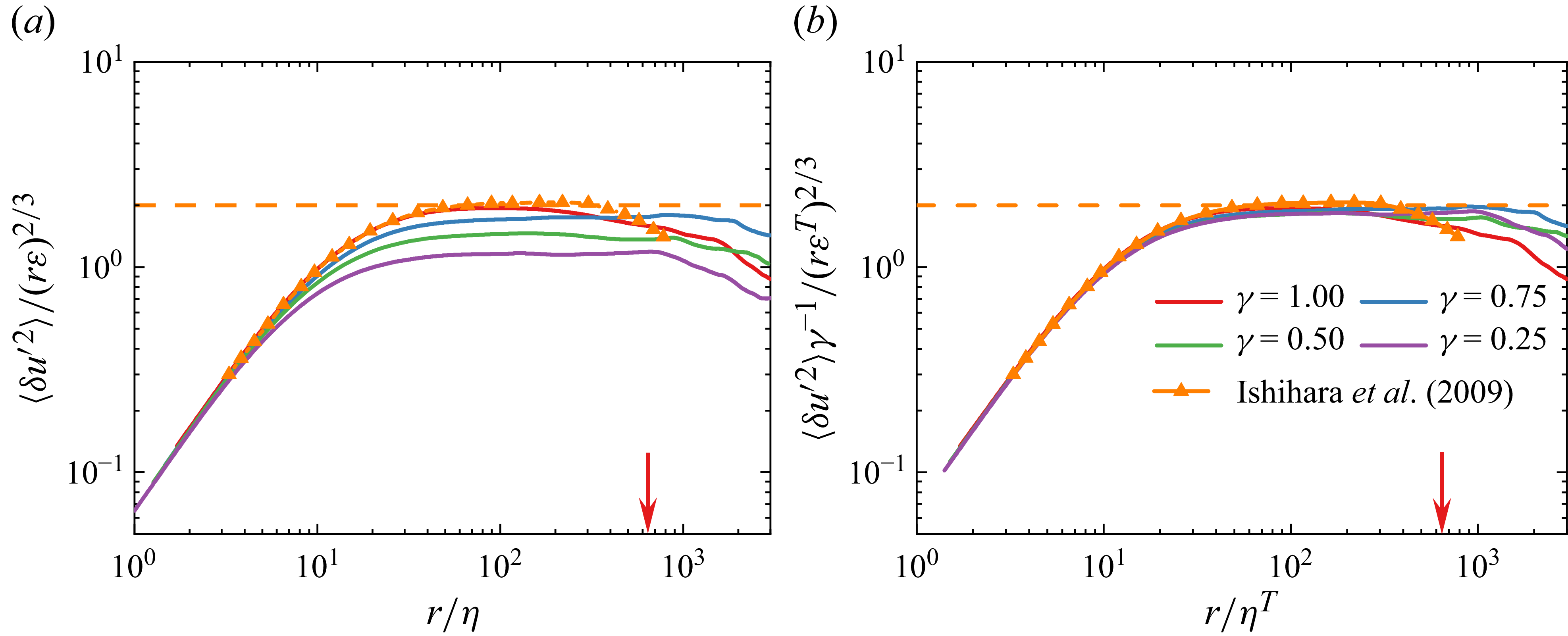
 ReH=105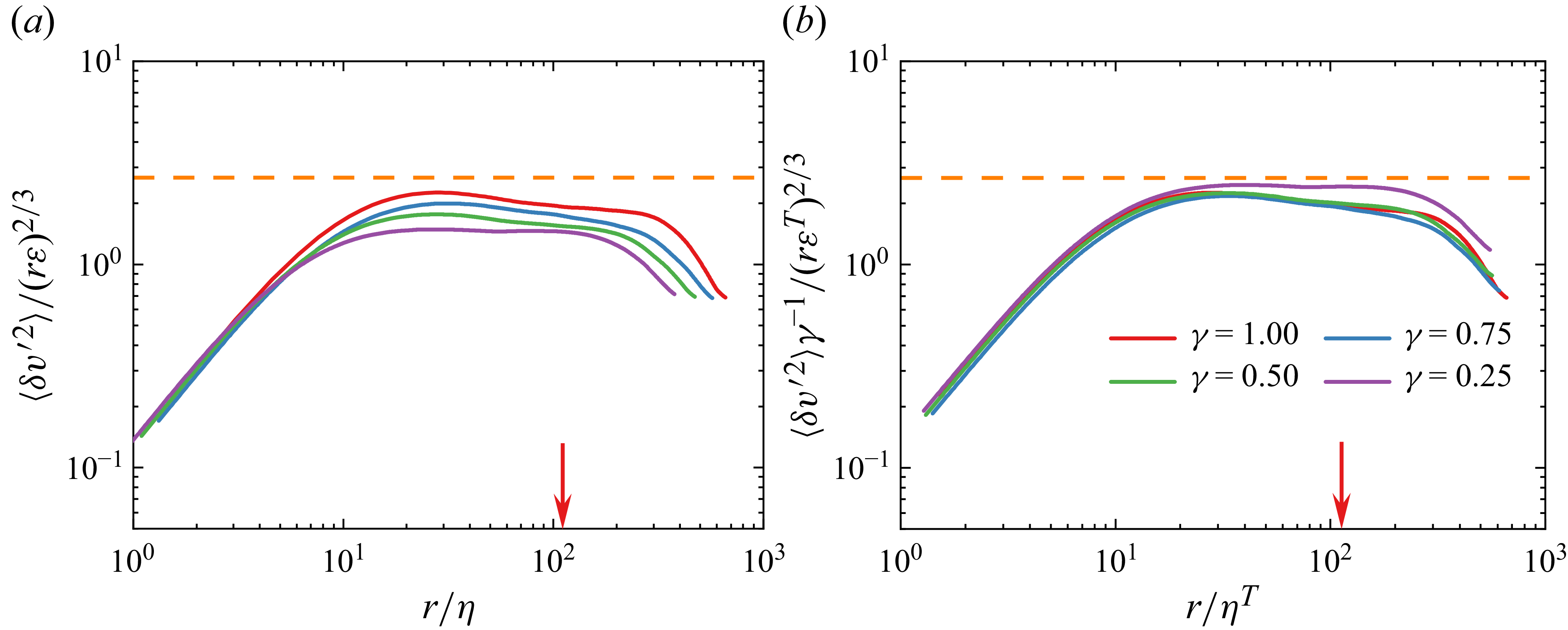
 η
η ε
ε ηT
ηT εT
εT ReH=104
 C2TSF
C2TSF ⟨δv′2⟩(r)/(εr)2/3=2.67
 L
L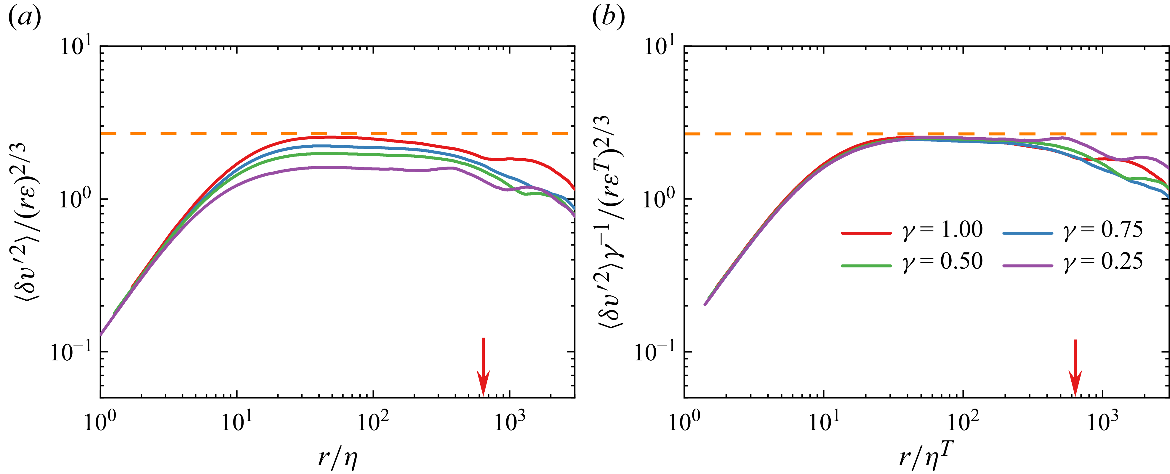
 ReH=105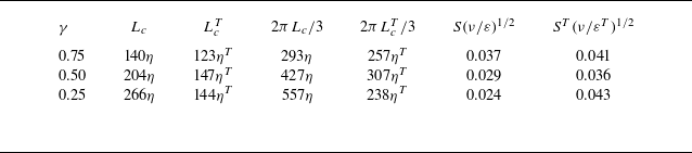
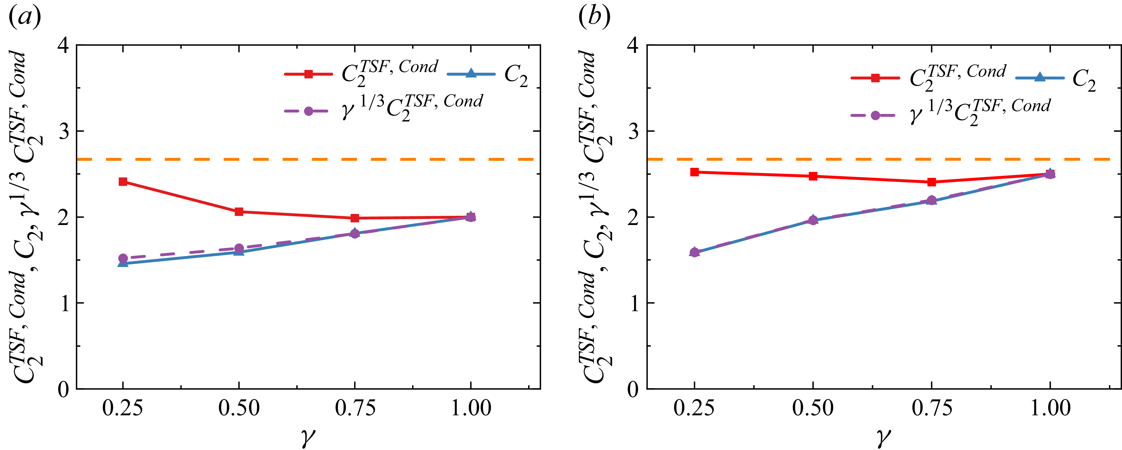
 C2TSF
C2TSF C2TSF,Cond
 γ
γ γ1/3C2TSF,Cond
 ReH=104
 ReH=105
 C2TSF
C2TSF ⟨δv′2⟩(r)/(εr)2/3=2.67
 ReH=104
 C4LSF
C4LSF C6LSF
C6LSF
 ReH=105
 |ω|th=0.14⟨|ω|⟩C
 ReH=104
 ReH=105
 η
η ε
ε ηT
ηT εT
εT ReH=104
 Reλ=100
 ReH=105
 Reλ=471
 r
r 20%
20% r=λT
r=λT ReλT=100
 353
353 ReλT=100
 SF=20
SF=20 λT/ηT=151/4(ReλT)1/2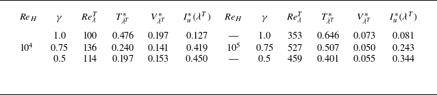
 TλT∗
TλT∗ VλT∗
VλT∗ Iu∗(λT)
 r=λT
r=λT γ=1.0
γ=1.0 0.75
0.75 0.5
0.5 ReH=104
 105
105 ReλT
ReλT
 γ=1.0
γ=1.0 ReλT=100
 353
353 103
103 104
104 105
105 ⟨δu′2⟩(r)/(rεT)2/3
 ⟨δv′2⟩(r)/(rεT)2/3
 −⟨δu′3⟩(r)/(rεT)
 Bn
Bn Cn
Cn Dn
Dn Fn
Fn u
u v
v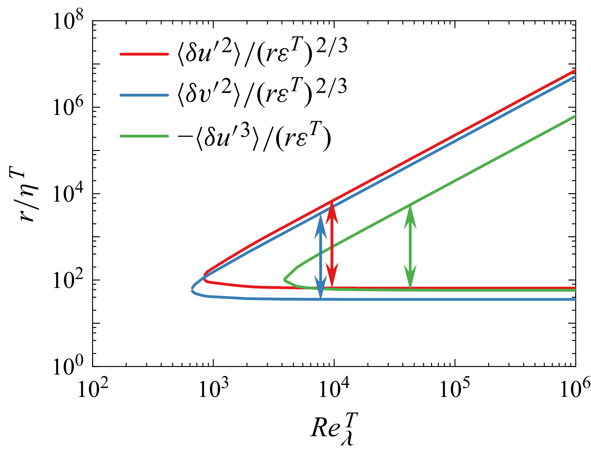
 r/ηT
r/ηT ⟨δu′2⟩
 ⟨δv′2⟩
 −⟨δu′3⟩
 2.00
2.00 2.66
2.66 0.798
0.798 2.5%
2.5% ReλT
ReλT Reλ
Reλ ⟨δu′2⟩(r)/(rεT)2/3
 ⟨δv′2⟩(r)/(rεT)2/3
 −⟨δu′3⟩(r)/(rεT)
 γ=0.5
γ=0.5 ReλT=114
 220
220 459
459 103
103 104
104 105
105 ⟨δu′2⟩(r)/(rεT)2/3
 ⟨δv′2⟩(r)/(rεT)2/3
 −⟨δu′3⟩(r)/(rεT)
 ReH=4×10⁴
 γ=0.5
γ=0.5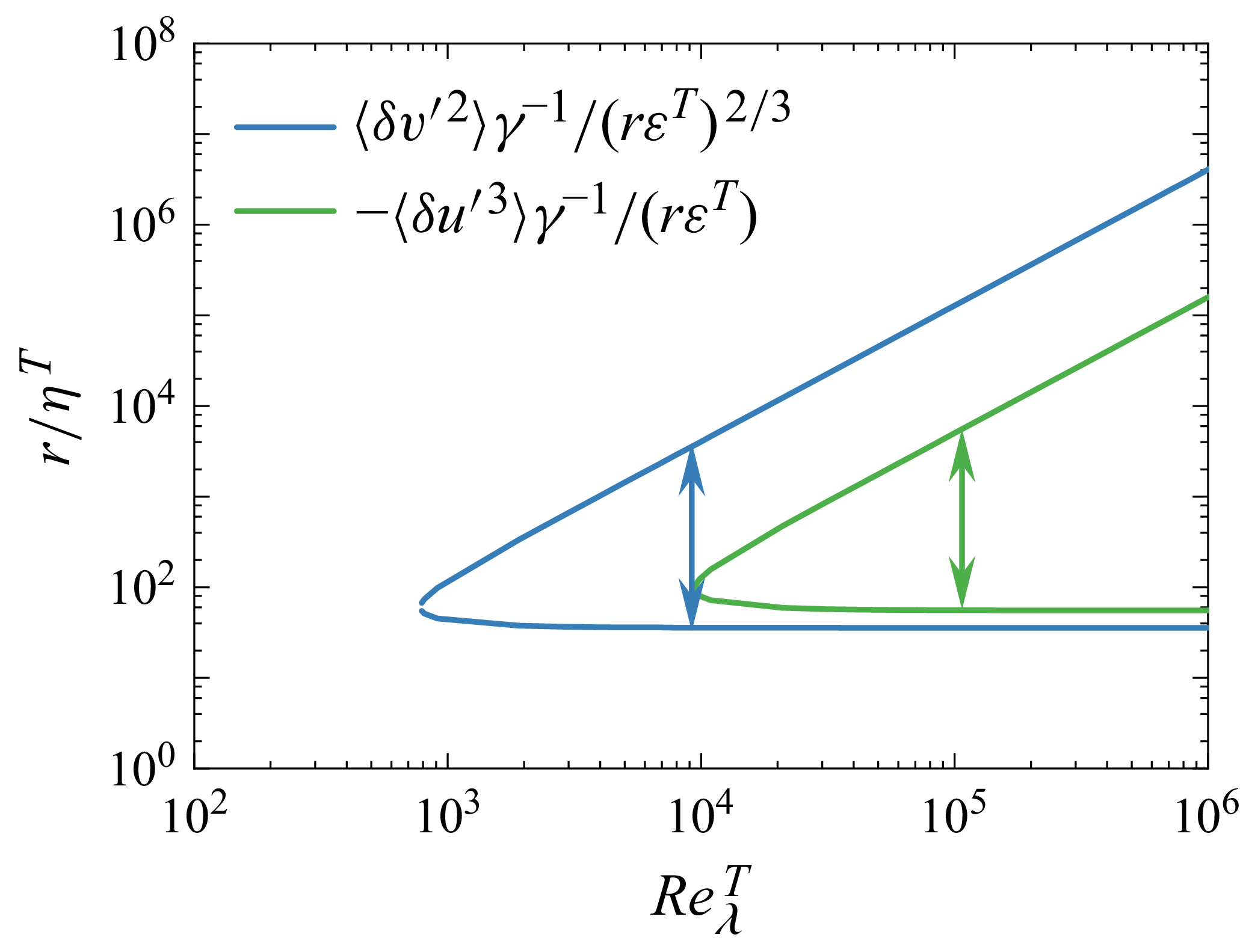
 γ=0.5
γ=0.5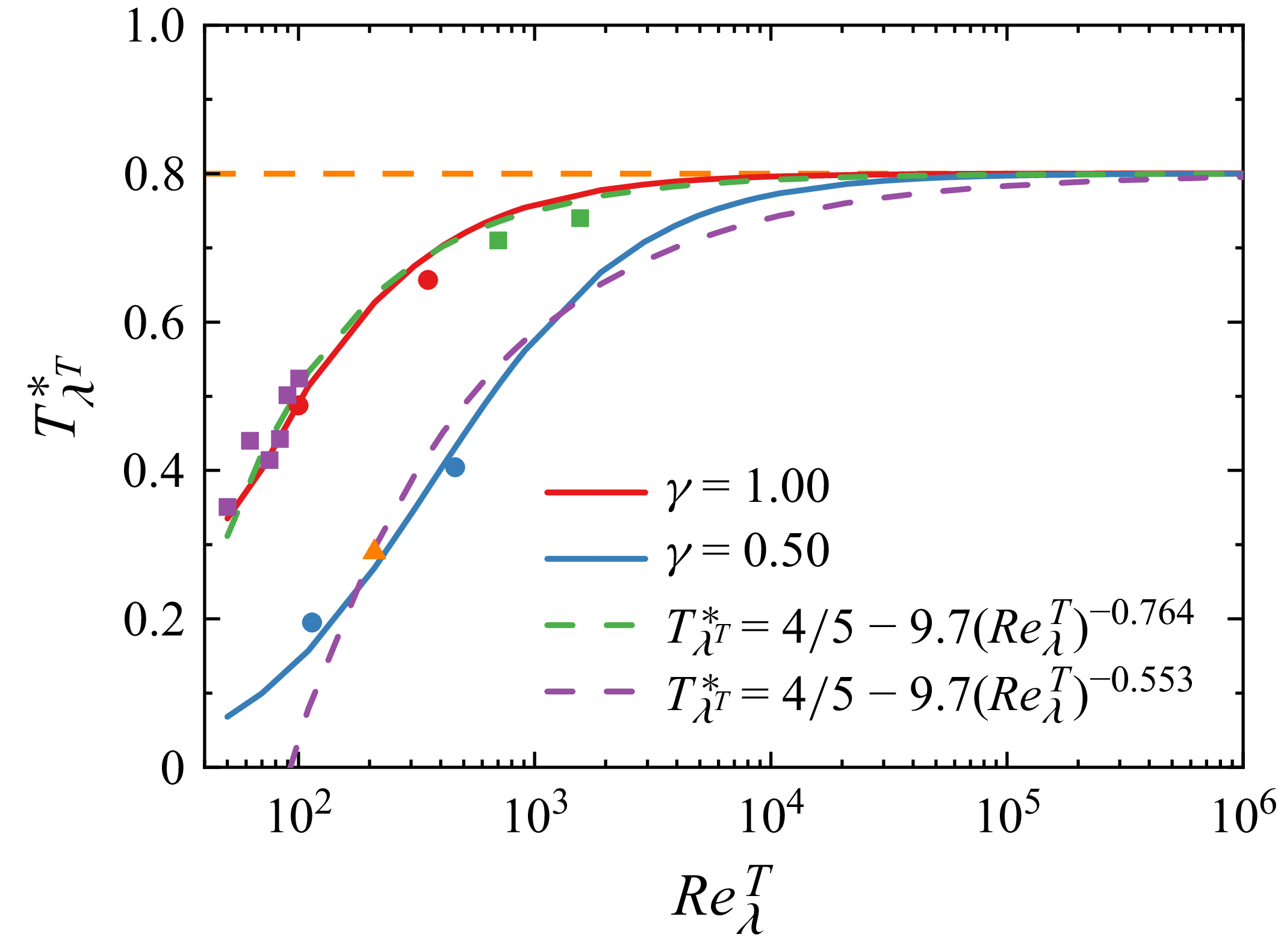
 TλT∗
TλT∗ ReλT
ReλT γ=0.5
γ=0.5 1.0
1.0 TλT∗=0.8
 γ=0.5
γ=0.5 ReH=4×10⁴
 γ=0.5
γ=0.5 ReH=104
 γ=0.5
γ=0.5 X
X Z
Z
 ReH=105
 γ=0.5
γ=0.5 ReH=105
 X
X Z
Z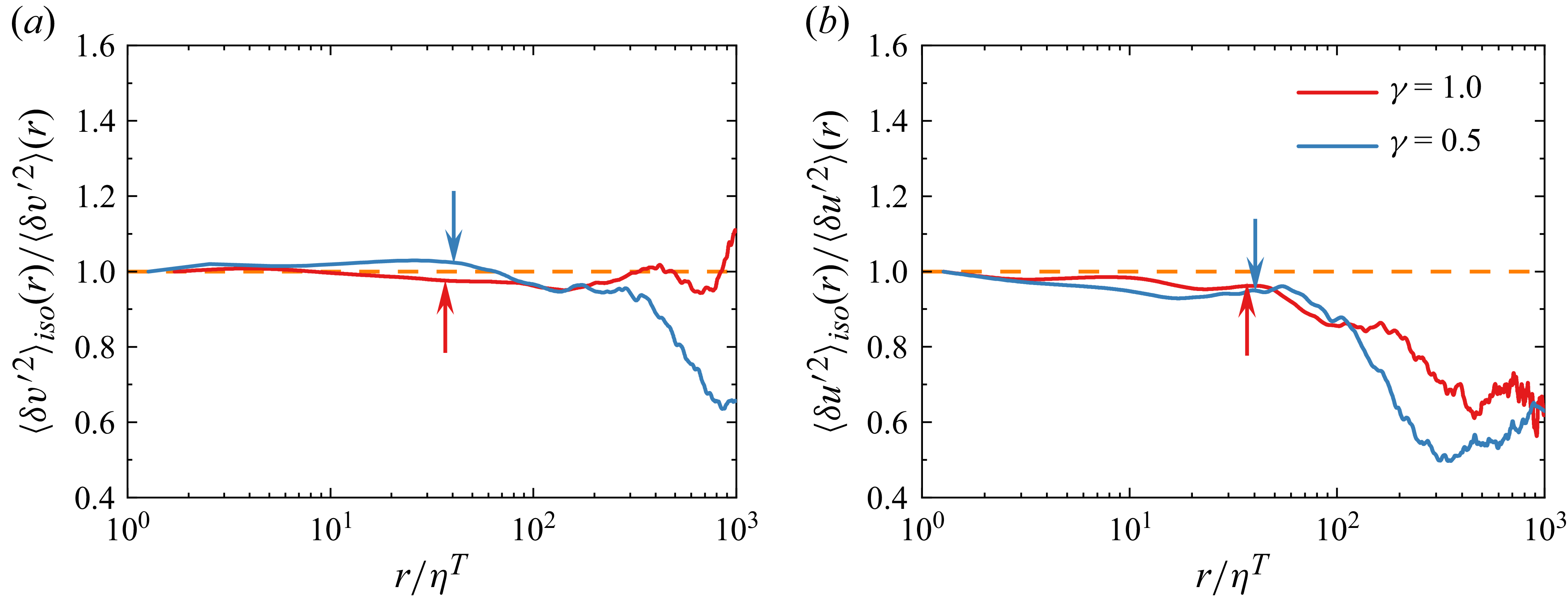
 ReH=105
 ⟨δv′2⟩iso(r)/⟨δv′2⟩(r)
 ⟨δu′2⟩iso(r)/⟨δu′2⟩(r)
 r
r 1
1 r=λT
r=λT

