


1. Introduction
The first radio-echo sounding (RES) systems used to image ice were fully analog, recording output on film with little or no post-processing (Waite, Reference Waite1959). With the advent of digital technologies, it became possible to record RES returns in simple, digital form by the mid-1970s (Goodman, Reference Goodman1975), which permitted basic post-processing. As the utility of ice-thickness data was recognized, glaciological RES data were acquired by many research groups by the 1980s, and by the 1990s, fully digital radar systems were being developed (Raju and others, Reference Raju, Xin and Moore1990). As these radar systems became sufficiently mature for regular data acquisition, RES collections proliferated. Moreover, by the 1990s, commercially available ground-penetrating radar systems, generally operating in very high-frequency (VHF; 30–300 MHz) bands, allowed new users to collect RES data without the overhead of building their own radar systems (e.g. Dallimore and Davis, Reference Dallimore, Davis and Pilon1992; Arcone and others, Reference Arcone, Lawson and Delaney1995). By the mid-1990s, airborne ice-penetrating radar flights, which had previously been solely under the purview of national programs, were being collected by individual science groups (e.g. Gogineni and others, Reference Gogineni, Legarsky and Thomas1998; Holt, Reference Holt2001). Today, vast quantities of RES data are now routinely collected over the ice sheets and over glaciers, and all are stored in digital form, permitting post-processing to enhance signal-to-noise ratio, geolocation or readability, and allowing easy extraction of quantitative geometric and radiometric information from the radar returns. Many of these data are collected using airborne chirped or frequency modulated continuous waveform radar systems, which require a different processing flow than that for impulse radars and are usually distributed as fully processed and interpreted products (Paden and others, Reference Paden, Li, Leuschen, Rodriguez-Morales and Hale2018). As opposed to these systems, which modulate the transmit frequency over a long or continuous transmit pulse then recover returns through complex signal processing, impulse radar systems transmit a short, simple burst of relatively broadband energy, with the frequency of the transmitted waveform set by the antenna characteristics. Ground-based impulse RES data are commonly acquired by individual research groups, which then use diverse processing flows and interpretation methods. Furthermore, due to the recent proliferation of airborne drone technology and commercial impulse radars designed to be deployed on these drones (e.g. RadarTeam Cobra), collection of airborne impulse radar data by individual groups is becoming more common, which also requires processing by those users.
While most commercial impulse RES systems have associated processing software (e.g. RADAN® for GSSI, or EKKO_Project™ for PulseEKKO), and there are several multi-system commercial processors (e.g. IXGPR and ReflexW), a number of drawbacks hinder their adoption as a common processing standard in glaciology. First, these programs are not free and often require per-user licensing that can significantly increase the total cost of using and maintaining a radar system. Second, these programs do not always provide the transparency required for scientific applications; for example, the exact algorithms used for filtering may not be described clearly, potentially obscuring effects on quantitative information about return power and impeding processing reproducibility by other groups using other software. Third, if any desired processing is not provided in the commercial software (e.g. depth-variable permittivity, complex data visualization, integrated interpretation, etc.), the user is left to ingest the output into an external program for these additional steps, potentially mitigating any convenience that the commercial software initially provided. Fourth, for the collection-system-specific software, processing data from multiple systems are unnecessarily complicated; often identical processing steps are desired for two different datasets, but collection-system differences might necessitate fully separate processing flows. Finally, these programs are often platform-specific (e.g. Windows only), preventing convenient installation for many scientific users.
Considering the deficiencies of commercial options, a number of customized programs have been developed to process glaciological RES data. These programs have been born out of necessity, in the case of processors for data in custom formats from purpose-built radar systems, or to avoid the drawbacks of commercial systems. However, research groups have largely written software specific to the output of their radars, often with no ability to ingest data from other collection systems, and these tools have not been widely shared. While processing algorithms for other types of RES data (chirped, frequency modulated continuous wave) are extensively documented and are publicly available (CReSIS, 2019), to our knowledge, there has only been one effort to publicly distribute a radar processing program for the impulse radar data that are often collected during ground-based field campaigns (irlib; Wilson, Reference Wilson2012a, Reference Wilson2012b). Although irlib provides a wide suite of processing functions, it has not seen widespread adoption by the glaciology community, perhaps due to its limited support of different input formats or lack of knowledge within the community about its availability.
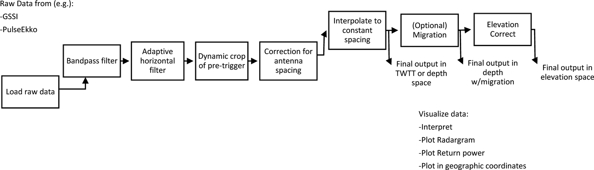
Despite the lack of a community standard for processing software, the processing chain itself has mostly been standardized (see Fig. 1 for a schematic of the standard processing chain), largely following established techniques for common-offset active-source seismic processing. After the raw data are converted to an accessible format, several filtering steps can be applied, most commonly the removal of low-frequency instrument noise and high-frequency environmental noise thought to be unassociated with the properties of the subsurface. The surface is typically ‘zeroed’ to remove returns above the ice surface. Final steps involve conversions from variable to constant trace spacing in the spatial dimension. Optionally, the two-way travel time (TWTT) of the radar wave can be converted to a depth below the surface using the speed of light in ice, potentially accounting for variable radar wave speeds (e.g. due to density variations in the firn) and the triangular travel path of the radar wave if there is a separation between the transmitting and receiving antennas. GNSS data can be used to position the traces to a constant spacing via interpolation, removing unwanted effects caused by spatial variability in data collection rate (e.g. sections of repeated measurement due to a pause during towing the radar). Data with constant horizontal spacing can then be ‘migrated’ to account for the true position of along-track but off-nadir reflections.
Summary of processing steps typically applied to radar data. All steps listed here are implemented in ImpDAR, often with multiple options for how the processing is performed.
After processing, the data are interpreted, a semi-subjective process that commonly focuses upon identifying and tracing reflecting horizons. Depending on radar frequency and depth within the ice column, reflections can be caused by different physical properties of the subsurface. Above the firn–ice transition, variations in density resulting from variable accumulation or formation of surface or depth hoar can result in sufficient change in permittivity to cause significant reflections (Arcone and others, Reference Arcone, Spikes, Hamilton and Mayewski2004, Reference Arcone, Spikes and Hamilton2005; Spikes and others, Reference Spikes, Hamilton, Arcone, Kaspari and Mayewski2004). Below the firn–ice transition, density is too uniform to cause enough permittivity contrast for a reflection (e.g. Harrison, Reference Harrison1973). At these greater depths, conductivity contrasts due to variations in chemistry, e.g. from volcanism or variations in dust, are thought to be the primary source of reflections (Hammer, Reference Hammer1980), though permittivity contrasts due to ice crystal-orientation fabric may also create internal reflecting horizons (Harrison, Reference Harrison1973). In high-frequency (HF; ~1–30 MHz) systems, the most notable reflection is often the ice–bed interface, which is usually a strong return due to the relatively large contrast in permittivity between ice and the rock, till or water that underlies it. Digitizing these layers is usually an interactive process with significant user input, either fully manual (simply drawing layers on an echogram) or semi-manual with simple, purpose-designed tools. These tools use simple algorithms to connect user clicks, for example, calculating the maximum return of each trace between the user inputs.
Here, we present ImpDAR, an open-source implementation of the standard impulse radar processing chain with an easy-to-use interface for interpreting the processed data. Many of the core processing algorithms are based on the St. Olaf deep radar processor, which was written in Matlab. Despite a long history of development and use in processing data (e.g. Welch and Jacobel, Reference Welch and Jacobel2003; Christianson and others, Reference Christianson2014, Reference Christianson2016), it was never publicly distributed. While none of the processing algorithms in ImpDAR are novel, their collection into a single, open-source, cross-platform and multiple-input format package is new. This freely available software has the potential to provide an important resource for glaciologists working with ice-penetrating radar data, particularly for radar-processing novices. We illustrate the utility of this software through application to two largely different glaciological datasets: one penetrating the full ice thickness in the interior of an ice sheet (Northeast Greenland Ice Stream; hereafter NEGIS) and one shallow collection imaging mainly snow and firn on a mountain glacier (South Cascade Glacier, Washington, USA). The similar processing chains between these two datasets illustrate the utility of having common processing software, while the differences between the datasets give a sense of the range of tasks to which this software can be applied.
2. Methods
Rather than focus on our exact implementation of the standard radar processing algorithms, we demonstrate the capabilities of ImpDAR by processing two example RES datasets. Where we have implemented additional options for processing, we describe those alternatives to provide guidance for other applications.
2.1. Datasets
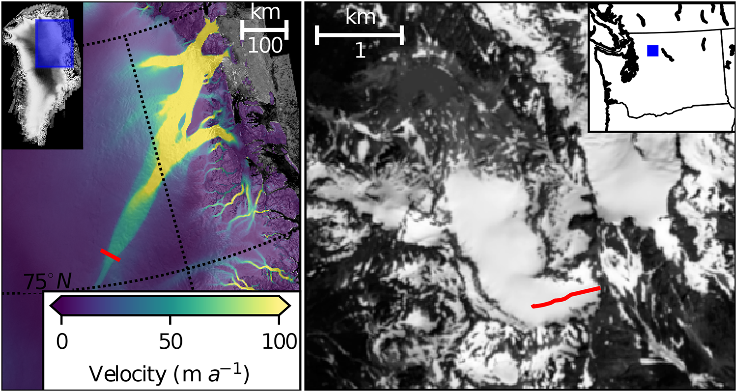
Figure 2 shows the collection sites for the two datasets, for which data collection methods differed significantly as we now describe.
Location of the two radar profiles. (a) Profile in Northeast Greenland plotted atop ice-flow speeds (Joughin and others, Reference Joughin, Smith and Howat2018). Blue box on inset shows the location of larger panel atop a mosaic of Radarsat images (Joughin and others, Reference Joughin, Smith, Howat, Moon and Scambos2016). (b) Profile on South Cascade Glacier (red) plotted atop Landsat-8 imagery. Small, blue box on inset shows the location of the main panel in Washington State.
2.1.1. NEGIS data collection
NEGIS has been a target of glaciological studies for over two decades (e.g. Fahnestock and others, Reference Fahnestock, Bindschadler, Kwok and Jezek1993; Joughin and others, Reference Joughin, Fahnestock, MacAyeal, Bamber and Gogineni2001; Mouginot and others, Reference Mouginot2015), both because it drains more than a tenth of the Greenland Ice Sheet (Rignot and Mouginot, Reference Rignot and Mouginot2012) and because it is enigmatic, as the sole outlet of the Greenland Ice Sheet where rapid, streaming ice flow extends hundreds of kilometers inland. The radar profile we present is part of a previously published and extensively studied survey of NEGIS (Christianson and others, Reference Christianson2014; Keisling and others, Reference Keisling2014; Vallelonga and others, Reference Vallelonga2014; Holschuh and others, Reference Holschuh, Lilien and Christianson2019; Riverman and others, Reference Riverman2019a, Reference Riverman2019b). The profile runs transverse to ice flow and spans the fast-flowing portion of the ice stream, capturing both incipient shear margins. The data were collected in 2012 using a custom-built HF system (Christianson and others, Reference Christianson2016) towed behind a snowmobile traveling ~10 km h−1. The center frequency was 3 MHz with ~2 MHz bandwidth, which necessitates large antennas and therefore large transmitter–receiver separation (~170 m).
2.1.2. South cascade data collection
South Cascade Glacier is a small mountain glacier that has an extensive history of scientific study (e.g. Krimmel, Reference Krimmel1989; Fountain, Reference Fountain1994), in part due to its status as a USGS benchmark glacier (Meier, Reference Meier1961; O'Neel and others, Reference O'Neel2019). Seasonal mass-balance surveys have been performed here every spring and fall since 1959. The radar profile we present was collected in spring 2017 using a commercial VHF PulseEKKO Pro system. The radar was towed between two skiers, resulting in variable travel rate of ~3–5 km h−1. The center frequency was 500 MHz with small antenna separation (~15 cm) within a housing that is topped with a metal ground plane to reflect energy downwards.
2.2. Processing
Because the processing flow was nearly identical for the NEGIS and South Cascade datasets, we describe their processing together and note differences where applicable. The code for all processing is provided in Supplementary Material S2.
2.2.1. Data ingestion
Outputs from radar systems differ by manufacturer and by hardware version, necessitating a variety of methodologies for ingesting data. While we only demonstrate the use of this software with input data from two systems, only one keyword must be changed to process data from GSSI, PulseEkko, RAMAC or Blue Systems commercial radars, from Gecko or DELORES custom systems, or from gprMAX and SeidarT waveform modeling. In principle, common-offset radar data (i.e. those acquired with a fixed transmitter–receiver separation) have a relatively simple format. Since the 1980s, impulse radar systems digitize the wave returned from a transmitted impulse (Jacobel and others, Reference Jacobel, Anderson and Rioux1988), recording a number (often thousands) of samples at a fixed time interval (~10−10–10−8 s) for each reflected waveform (termed a trace). Traces are generally produced at a fixed interval (~10−6–10−4 s), sufficiently spaced both to prevent overlap in returned wave with the previous trace and also to prevent overwhelming the sampling rate of the digitizer. Hereafter, we distinguish these with the common terminology of ‘fast time’ for the sampling dimension and ‘slow time’ for the trace dimension. Typically, before writing to disk, tens to thousands of traces are averaged, or ‘stacked,’ to reduce noise and file size while maintaining reasonable spatial resolution. Thus, the resulting data naturally form a 2 d array, with each column representing a (likely stacked) trace, or single record in slow time and horizontal space, and each row representing the wave amplitude at a fixed interval in fast time after the initiation of digitization. If multiple channels (parallel data streams, possibly recorded in different frequency bands, with multiple antennas, with signal amplifiers and/or attenuators, or with different dynamic ranges) are recorded, the data array gains a third dimension. Along with this data array, output files from radar systems usually store ancillary information about collection methods (e.g. transmitter and sampling frequencies), fast times, slow times and geospatial information.
Due to the logistics of collection, such as limited time in the field, limited storage or limited battery capacity, and propensity for interruption of data collection due to power outages or other operational problems, radar profiles are often partitioned into many smaller segments. These discontinuous data must be spliced back together, through operations such as trimming a profile, concatenation, reversal of a profile or some combination of these processes. For the NEGIS profile, we spliced together 32 separate files to form a ~41 km profile and for South Cascade Glacier, we concatenated two profiles to create a single, ~0.8 km profile.
2.2.2. Vertical bandpass filtering
The first processing steps attempt to improve the signal-to-noise ratio of the returns. The energy transmitted by an impulse radar system is concentrated around some center frequency, in our case ~3 MHz with ~2 MHz bandwidth for the NEGIS data and 500 MHz with ~100 MHz bandwidth for the South Cascade Glacier data. In the case of impulse systems, the bandwidth usually refers to the region in which the transmitted power is a significant fraction of the peak transmit power, which is generally constrained by the antenna characteristics. The bandwidths reported here are estimates of where the power is at least 10% of the peak power, based on the spectra of the returns.
Frequencies are not generally converted in the subsurface, so variability in wave amplitude outside these frequencies is generally assumed to be noise. Long-wavelength noise (relative to the operating frequency of the radar) is generally associated with the ringing of the receive antenna induced by the transmitter, termed ‘wow,’ (see Fig. 3c for an example). Short-wavelength noise (again relative to the radar's operating frequency) is induced by environmental variability and through the limits of measurement precision. Usually, the amplitude of both types of noise must be minimized in order to avoid overwhelming the desired returns. In certain cases, it may be desirable to filter away from the center frequency of the radar (e.g. Woodward and King, Reference Woodward and King2009), and ImpDAR permits the user to perform such filtering, though the signal-to-noise ratio is usually maximized by filtering around the center frequency. For the data presented here, we do this using a 5th-order zero-phase (forward–backward) Butterworth filter, with passband around the transmitted frequencies: 1–5 MHz for NEGIS and 300–700 MHz for South Cascade Glacier. The effect of this filtering can be seen by comparing Figures 3c and d or 4d and e. The Butterworth filter is chosen because it has flat gain in the passband, though care must be taken that the drop off is not so steep that the filter introduces ringing outside the pass band. ImpDAR also implements two other finite impulse response filters, Chebyshev type-I and Bessel, both of which have tradeoffs in the flatness of the gain and the cutoff range compared to the Butterworth filter, but may be more effective for some datasets. The order of each of these filters can be adjusted, so users can easily experiment to determine which filter and order work best for a particular dataset. For a comparison of these filters and their effect on the data from NEGIS, see Supplementary Figure S2.
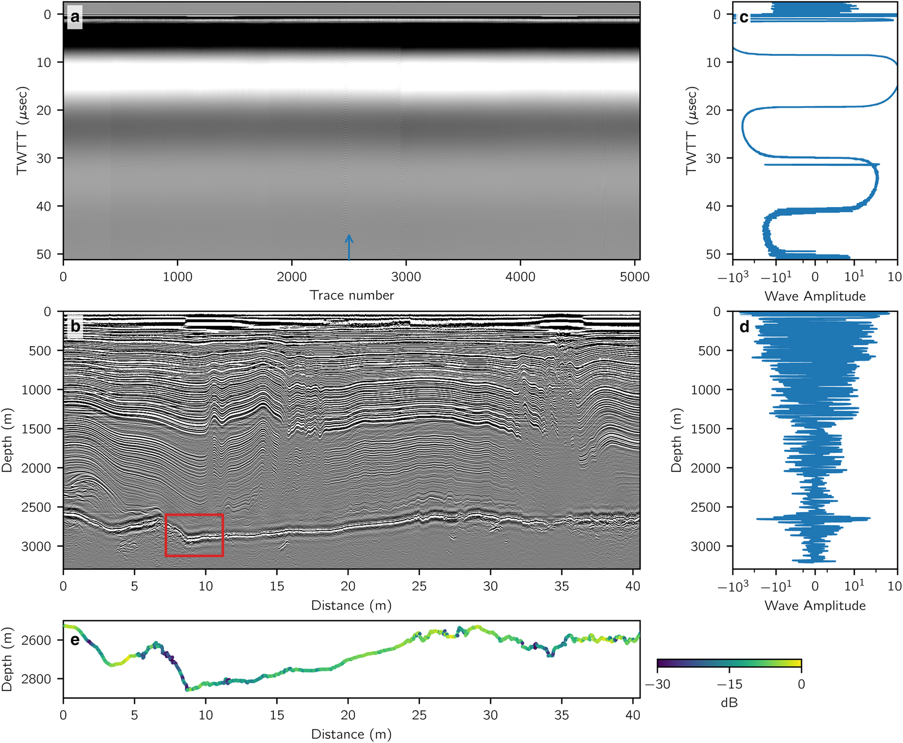
RES profile from the Northeast Greenland Ice Stream. (a) Radargram before processing. Arrow indicates the location of traces plotted in (c, d). (b) As in (a), but after all processing steps. Note the change in axes from two-way travel time vs trace number to depth vs along-track distance as a result of processing. The red box shows area used for migration comparison in Figure 5. (c, d) Wave amplitude vs two-way travel time before processing (c) or depth after processing (d) for trace indicated by an arrow in (a); the processed trace is plotted before conversion to geographic coordinates to preserve direct comparison. Note the successful removal of the ‘wow’ by the vertical bandpass filter. (e) Return power of the semi-manually picked bed reflection. Compare to Figure 4 in Christianson and others (Reference Christianson2014) to see consistency between users’ picks and processing chains.
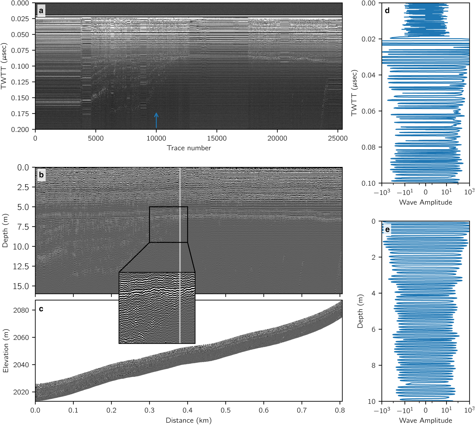
RES profile collected on South Cascade Glacier. (a) Radargram before processing. Arrow indicates the location of traces plotted in (d, e). (b) As in (a), but after all processing steps except elevation correction (note differing axes as a result of processing). Vertical gray line approximates the equilibrium line. Zoomed inset shows the bright reflection of the previous summer's surface, with past summer surfaces ascending to meet it at the equilibrium line at ~0.375 km. (c) As in (b), but corrected for variable surface elevations. (d, e) Wave amplitude vs depth for trace indicated by an arrow in (a), before and after processing. Y-axes are clipped to enhance readability.
2.2.3. Horizontal filtering
An additional strategy for removing noise is to subtract an average trace or something akin to it. In simplest form, this would remove perfectly flat reflectors, which are often thought to be artifacts (e.g. a reflection from some surface object that stays a fixed distance from the radar system) and can remove surface ringing. However, care must be taken to preserve real horizontal reflectors, such as subglacial lakes, so often this filtering is tapered to affect only the shallow subsurface. By choosing to remove something other than the average trace calculated over the entire profile, for example, an average in a moving window around a given trace or a filtered average, artifacts with minor tilt can also be removed. In any of these cases, the strength of the subtracted trace is usually tapered to leave deep, weaker reflections unaltered. ImpDAR implements several horizontal filtering options. For the Northeast Greenland data, we used an adaptive horizontal filter that subtracts the average low-frequency component of the 100 traces surrounding each given trace. This adaptive filtering generally leaves real reflectors unperturbed, even if they are relatively flat, while removing artifacts (see Supplementary Fig. S2 for a detailed view of the effect of this filter). For the South Cascade data, we subtracted an average trace from a typical portion of the profile. The horizontal filtering step can also be done later, after moving the traces to constant spacing, to make sure the effect of the filter is constant in space, though this makes little practical difference.
2.2.4. Time-zero
We next remove data recorded before the arrival of the air wave (the direct arrival of the transmitted pulse from the transmitting to the receiving antenna). These returns exist in custom data because they are used to trigger the recording of the radar system, and they are intentionally preserved even in the PulseEkko system to ensure that no subsurface data are missed. In both raw radargrams (Figs 3a and 4a), the returns before the arrival of the air wave are characterized by very small wave amplitude, which is associated with system and environmental noise. This is particularly visible in any individual trace (above 0 μs in Fig. 3c and above 0.02 μs in Fig. 4d), where the wave amplitude is substantially smaller than that of reflections from interfaces in the subsurface. The data above the air wave returns are cropped, and the sample numbering and TWTT are updated to match this change in the surface.
2.2.5. Time-to-depth conversion
The user usually desires to convert the y-axis from TWTT (i.e. the fast time dimension) to depth, a multi-step process involving accounting for antenna separation, the spatial structure of permittivity of the ice/firn, and the effects of off-nadir reflections. Correcting for off-nadir reflections, termed migration, is discussed below since the antenna separation must be accounted for first. The time/depth conversion is straightforward if the speed of light in the medium is constant and the transmitting and receiving antennas are collocated. Despite real horizontal and vertical variations in permittivity through the firn/ice transition, when processing data, the permittivity of the firn and ice is often assumed to be constant (with a speed of light = 1.68 m s−1), or a spatially variable correction is applied to account for total firn air content on a trace-by-trace basis. In most commercial VHF radars, the antenna separation is generally small enough (~10 cm) that it can be neglected, so spatial variations in permittivity are easily accounted for since the transmitted and received waves follow the same ray path irrespective of any permittivity variations.
Correctly determining the depth of returns when the transmitting and receiving antennas are farther apart (e.g. 169.4 m in the case of the NEGIS data presented here) requires accounting for the travel time of the air wave between the transmitter and receiver and for the approximately triangular path taken by the radar wave through the subsurface. If the path taken by the radar wave is known, for example, if it is assumed to be a symmetrical triangle from source to receiver, accounting for variable wave speeds is again straightforward. This is a reasonable assumption as wave speed variations are generally strongest in the vertical, for example, because of density variations due to firn compaction, though weak enough that refraction does not drastically alter the wave path. Horizontal variations in wave speed on length scales shorter than the antenna separation would break the symmetry of locating the returns and complicate the wave path, but fortunately, horizontal variations in permittivity generally occur over larger spatial scales than the antenna separation.
ImpDAR's implementation of the antenna-separation correction handles variable transmitter–receiver separations and vertical variations in wave speed. At each sample depth, this correction is done using the root-mean-square velocity in the ice above that reflector; thus, vertical speed variations are accommodated in an average sense. Horizontal variations could be easily accommodated by treating each trace separately (assuming that the horizontal variations happen on length scales longer than the antenna separation), though we have not implemented such a feature since it is rare to have data with which to constrain such lateral variations. For the NEGIS data, we assume that the radar wave speed is a constant 1.68 × 10⁸ m s−1 when performing the antenna-separation correction. For the data from South Cascade, we account for the variations in firn density by using a dielectric mixing model (Wilhelms, Reference Wilhelms2005) with input from several firn cores drilled in 2017–2018.
2.2.6. Geolocation
Similar to the fast-time-to-depth conversion, data are normally collected with roughly constant trace spacing in slow time, but data are most easily interpreted and utilized in the spatial domain. Often, a GPS-produced NMEA (National Marine Electronics Association) string is used for basic geolocation, but unless a real-time kinematic correction is applied, these GPS data are insufficiently precise for many scientific applications. Integrating noisy data can result in the appearance of motion when the receiver is stationary. Noisy vertical positions may give the false impression of an uneven surface and thus, if the data are elevation corrected, of uneven layers. To overcome these shortcomings, many radar collections use an external, dual-frequency GNSS receiver; the dual-frequency GNSS data can then be post-processed to increase accuracy and precision to centimeter level, and then can be used to precisely locate the traces.
To relocate the traces in the both datasets, we first interpolated the precise GNSS data (which were post-processed using differential carrier-phase positioning (e.g. Misra and Enge, Reference Misra and Enge2006) for NEGIS and precise point positioning for South Cascade Glacier (Chen and others, Reference Chen2004)) onto the traces using the assumption that the timestamp of each radar trace is precise; this is generally true because the radar system's clock is precise and can be accurately synchronized to the GPS-constellation time at the start of the data collection. Because the timestamp of the precision GPS is also synchronized exactly with the GPS-constellation time, we can then get accurate and precise locations for each trace. After finding the more precise positions of the traces, we do a simple linear interpolation to constant trace spacing (8 m for NEGIS and 10 cm for South Cascade Glacier), to avoid distortion from variable towing speeds during acquisition.
2.2.7. Migration
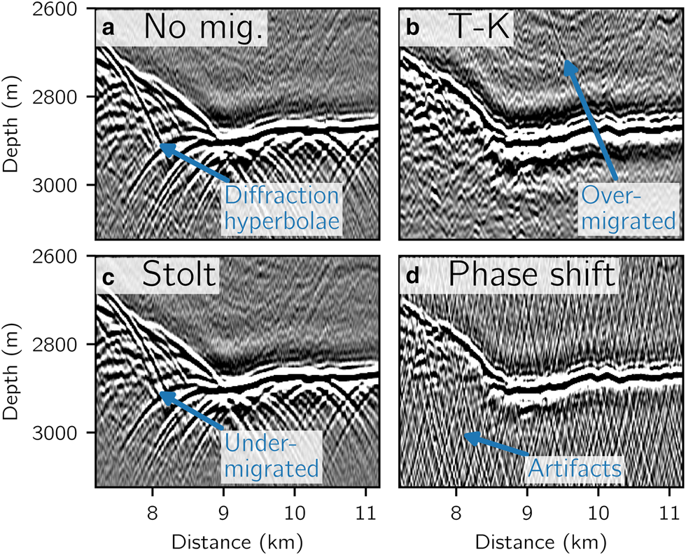
An important complication in interpreting RES data is determining where in the subsurface the interface that creates a reflection is located. Precise location of the collection system on the surface is not necessarily sufficient for this determination since off-nadir reflections, both along- and across-track, can cause the returned energy to come from directions that are not directly underneath the radar system. Across-track returns plague surveys along narrow glaciers (e.g. Conway and others, Reference Conway2009) or when the radar is flown high above the surface (e.g. Grima and others, Reference Grima, Kofman, Herique, Orosei and Seu2012). Correcting for across-track returns without an array of antennas oriented in the cross-track direction is exceedingly difficult, and most often data are interpreted without their removal. It is generally possible to correct along-track, off-nadir reflections in impulse radar data by utilizing geometric information in adjacent traces; more complex steps allow similar along-track focusing of chirped RES data (e.g. Legarsky and others, Reference Legarsky, Gogineni and Akins2001). Active-source seismologists have developed a number of algorithms to perform the geometric-type migration that is applicable to impulse radar data (Claerbout, Reference Claerbout1985; Sheriff and Geldart, Reference Sheriff and Geldart1995). Here, we implement several of these seismological migration routines including integration along diffraction hyperbolae, known as diffraction-stacking or Kirchhoff migration (Schneider, Reference Schneider1978); frequency-wavenumber migration for both a basic interpolation in frequency-space (Stolt, Reference Stolt1978) as well as a downward-continuing phase-shift method (Gazdag, Reference Gazdag1978); and finally, time-wavenumber migration (Cohen and Stockwell, Reference Cohen and Stockwell2010). Kirchoff, frequency-wavenumber and phase-shift migration are implemented directly in ImpDAR, with options to use python's C interface to speed the computation of some critical steps; this C code is distributed both as a source and precompiled for common systems. Time-wavenumber migration leverages the open-source SeisUNIX package, which is written in C rather than Python, and thus is faster at the expense of requiring external compilation (Cohen and Stockwell, Reference Cohen and Stockwell2010). A comparison of the results of some of these different routines, illustrating the benefits and drawbacks of each, is shown in Figure 5. Trial-and-error indicates that the time-wavenumber migration in SeisUNIX and the phase-shift migration produced the best results. The NEGIS data presented in Figure 3 use the T-K migration. No diffraction hyperbolae were visible in the South Cascade profile, likely due to the inconsistency of reflectors in the shallow firn, so we left these data unmigrated.
Effects of migration on a reflector. Area is taken from the boxed region of Figure 3b, showing the bed reflector at NEGIS. (a) Data with no migration. The other panels show three of the five migration types that can be called from ImpDAR: (b) time-wavenumber, or T-K, processed using SeisUNIX (c) Stolt, or frequency-wavenumber, implemented directly in ImpDAR and is by far the fastest migration routine and (d) phase-shift migration, implemented directly in ImpDAR.
2.2.8. Interpretation
After processing, the user generally wants to extract useful quantitative information from the radargram by digitizing (or picking) reflectors. Picking is typically a semi-automated process, where the user interactively selects points on the reflected horizon while the software attempts to follow the reflector between the user-picked points, sometimes using wave frequency to isolate the portion of the waveform associated with a reflection from a discrete interface. The exact method for interpolating between user-identified points varies between different research groups. We have implemented a very simple function that iterates through traces and seeks a peak with a prescribed polarity within a frequency-dependent distance of the line segment connecting the two user picks. If the reflector has little curvature, this algorithm can follow the reflector for many traces with little user input, but significant curvature causes the picker to require more user input to trace the reflection faithfully. While this routine is simple, quick and effective for single reflectors, there is significant scope for developing more clever and automated algorithms to follow reflections, and ImpDAR is set up to readily accept alternative functions for interpolating between user picks, or for entirely automated picking. ImpDAR automatically calculates the strength of reflectors as they are picked. The power is calculated as the average squared wave amplitude of the samples spanned by the two peaks with opposite polarity surrounding the central peak. ImpDAR can then easily export reflector depth and power in geographic coordinates to enable further interpretation. It also provides several useful tools to aid in the interpretation process, such as easy graphical changes to the color palette and plotting of the depths of reflectors from other intersecting or contiguous profiles.
2.2.9. Elevation correction
The surface of the radar profile can optionally be corrected to match the variable elevation of the physical surface. This is generally done after all other processing steps, as it potentially renders the data inoperable for filters and other corrections. Figure 4c shows an example of a profile corrected to the variable surface, illustrating both the utility and the downsides of this step; while it is easier to identify how layers conform to surface topography, a highly variable surface elevation necessarily leads to empty space on a rectangular plot and thus can reduce overall readability.
3. Results
3.1. NEGIS
The processed radargram is shown in Figure 3b. The bed return is clearly visible at 2500–2800 m depth throughout the profile, and internal layers can be seen at most depths except in the shear margins where steep layer slopes cause a lack of returns (Holschuh and others, Reference Holschuh, Christianson and Anandakrishnan2014). The bed was picked based on the maximum amplitude return. These results can be compared to the previously processed and published radargrams from this survey (Christianson and others, Reference Christianson2014; Keisling and others, Reference Keisling2014; Vallelonga and others, Reference Vallelonga2014; Riverman and others, Reference Riverman2019b).
3.2. South Cascade Glacier
The processed profile of South Cascade Glacier is shown in Figure 4b, with the same profile elevation-corrected in Figure 4c. Perhaps the most salient feature of this profile is the previous season's summer surface at ~7 m depth. The equilibrium line is located at ~0.375 km, but surprisingly, the profile shows accumulation below this elevation and ablation above; previous summer surfaces ascend toward this point from the left, and the lack of discernable structure below this surface to the right is indicative of temperate ice. Similarly, non-elevation-dependent patterns of mass balance have been previously observed on South Cascade Glacier (Meier and Tangborn, Reference Meier and Tangborn1965), where in low snow years, accumulation may be confined to the southwest margin due to topographic shielding from the surrounding mountains, and previous work has shown accumulation to be highly dependent on surrounding topography on another comparable alpine glacier (Brown and others, Reference Brown, Harper and Humphrey2010; Florentine and others, Reference Florentine, Harper, Fagre, Moore and Peitzsch2018). In addition to summer surfaces, several crevasses and possible meltwater inclusions are visible in the temperate ice on the right side of the profile, and the steeply dipping bed, which is overlain in the field by a notable bergschrund, is visible at the far right.
4. Discussion
Here we provide additional context for the utility of the ImpDAR package and suggest further functionality that could be developed later.
4.1. Advantages of ImpDAR
The primary purpose of this software is to provide an open-source alternative to commercial radar processing software and proprietary processing chains used by individual researchers. The code is freely available, has been tested on MacOS, Windows and two flavors of Linux (Ubuntu and CentOS), and its dependencies, including the programming language, are all free. Compared to other open-source radar processing software, it supports a greater range of input formats and includes more interpretation utilities. Irlib (Wilson, Reference Wilson2012a) provides most of this functionality for a few input formats, and is a superb tool for processing and interpreting those data, but highlights the need for greater advertisement and community adoption of available software; most of our work was done without the knowledge of irlib, and therefore unnecessarily repeated that already available functionality. ImpDAR's documentation provides a number of examples of processing glaciological RES data, ranging from step-by-step examples for novices to specific functionality for experienced users; a basic example of data processing is provided in Supplementary Material S2. The functions used internally are also fully documented, allowing straightforward modification for specific use cases. Moreover, all the default values are set up for ice, allowing rapid preliminary data visualization without requiring the novice user to look up a large set of ice-specific parameters.
Installation of the software is made straightforward for new users through Anaconda (http://anaconda.com). Anaconda provides an easy-to-use python environment with most of the dependencies and provides straightforward tools for installing the other dependencies and a stable version of ImpDAR itself. Installation of a stable version with Anaconda requires only three steps with no prerequisites: (1) install Anaconda, (2) use Anaconda to install dependencies and (3) use pip (provided with anaconda) to install ImpDAR. Step-by-step instructions, with links and commands, are provided in Supplementary Material S1, as well as in the online documentation (see Acknowledgements).
4.2. Additional functionality
A key advantage of open-source software is the ease of adding additional functionality suited to the needs of particular users. While ImpDAR is functionally complete for the most common radar processing tasks, we have added some additional functionality, and other useful processing tools could be easily added.
In addition to the ability to process real RES data, we have implemented compatibility with gprMax, a synthetic radar waveform modeling package (Warren and others, Reference Warren, Giannopoulos and Giannakis2016). This compatibility allows easy ingestion of synthetic radargrams and thus straightforward comparisons between real and synthetic data while using identical processing chains.
While the processor has been developed for common-offset data, where the data are essentially an array of wave amplitude in two spatial or temporal dimensions, the processing algorithms are largely applicable to other ice-penetrating radar collection methods that can also be conceptualized as an array of wave amplitudes. For example, common-midpoint (CMP, also called move-out) collections can be visualized as a radargram in offset distance vs TWTT space, then similar processing steps can be used to filter the data. While we have not implemented any plotting or processing specific to these other collection methods, a user would only have to load the data into an array before performing common operations upon it with ImpDAR.
The similarity between seismic and RES data offers extensive opportunities to leverage processing techniques and tools developed for active-source seismics for use with glaciological RES data. The use of seismics in oil and gas reservoir exploration has led to a comparative wealth of such tools (Forel and others, Reference Forel, Benz and Pennington2005; Schlumberger, 2019), some of which have been utilized in glaciology (e.g. Bingham and others, Reference Bingham2017). We have taken advantage of the fast migration routines provided by the open-source package SeisUNIX, but there is a large potential for other applications, even simply through further interfacing with SeisUNIX.
The need to pick all but the flattest reflecting horizons semi-manually presents a significant barrier to utilizing the wealth of information in each radargram. Picking in ImpDAR was designed to be modular, so that other algorithms could easily be utilized. There have been a number of efforts to automate picking internal reflectors (Fahnestock and others, Reference Fahnestock, Abdalati, Luo and Gogineni2001; Sime and others, Reference Sime, Hindmarsh and Corr2011; Mitchell and others, Reference Mitchell, Crandall, Fox and Paden2013; Onana and others, Reference Onana, Koenig, Ruth, Studinger and Harbeck2014; Panton and Karlsson, Reference Panton and Karlsson2015; Xiong and others, Reference Xiong, Muller and Carretero2017; Delf and others, Reference Delf, Schroeder, Curtis, Giannopoulos and Bingham2020), the basal reflection (Gifford and others, Reference Gifford2010; Crandall and others, Reference Crandall, Fox and Paden2012; Ilisei and others, Reference Ilisei, Ferro and Bruzzone2012; Kamangir and others, Reference Kamangir, Rahnemoonfar, Dobbs, Paden and Fox2018) and reflections in Martian ice (Freeman and others, Reference Freeman, Bovik and Holt2010; Ferro and Bruzzone, Reference Ferro and Bruzzone2013). Some of these algorithms leverage machine-learning techniques, which have been used to find surface and bed returns (Crandall and others, Reference Crandall, Fox and Paden2012; Kamangir and others, Reference Kamangir, Rahnemoonfar, Dobbs, Paden and Fox2018) and to extract multiple internal reflectors (Ferro and Bruzzone, Reference Ferro and Bruzzone2013; Mitchell and others, Reference Mitchell, Crandall, Fox and Paden2013). Despite the extensive work on automatic layer picking, in practice most interpretation continues to be at least semi-manual. ImpDAR provides a framework on top of which existing or new automatic picking algorithms could be implemented, and we are actively working on an automatic picker for a future release.
5. Conclusions
We have developed an open-source impulse radar processor and interpreter capable of handling RES data collected with a number of common radar systems. Its utility is demonstrated through the processing of two largely different but representative RES datasets from ice-sheet and mountain glacier settings. This processing software aims to make radar processing and interpretation more accessible to novice users, while still providing the full suite of functionality required for complex use cases, such as quantitative analysis of return power, migration or sophisticated geospatial operations. Although the processing algorithms implemented here are not novel, their collection into a single, freely available framework with the capability to handle a variety of input formats is new. Additional functionality will be added in the future to expand the program's applications, but in current form, it provides an implementation of all the most common processing operations for researchers collecting ice-penetrating radar data.
Supplementary material
The supplementary material for this article can be found at https://doi.org/10.1017/aog.2020.44
Data avalailablity
ImpDAR is freely available at https://www.github.com/dlilien/ImpDAR. Documentation can be found at https://impdar.readthedocs.io/en/v1.0.1/. The release corresponding to this publication is frozen at http://doi.org/10.5281/zenodo.3833057.
Acknowledgements
We thank the NEGIS and South Cascade Glacier field teams who collected the radar profiles. The U.S. National Science Foundation (award PLR-0424589) supported the NEGIS fieldwork and the United States Geological Survey and the University of Washington supported the South Cascade Glacier fieldwork. We also thank Brian Welch and many St. Olaf College undergraduate students who developed Matlab routines for radar processing over the last three decades that serve as the basis for ImpDAR, particularly Logan Smith who worked on the first auto picker. BH, KC, JD were supported by the National Science Foundation through awards PLR-1744649, PLR-1643353, and PLR-1503907. DL was partially supported by the National Science Foundation through PLR-1443471. Additional support was provided to JD through the Washington NASA Space Grant Consortium.


 Open access