Tracing Henkel’s ‘visibility limit’ in archaeological scholarship

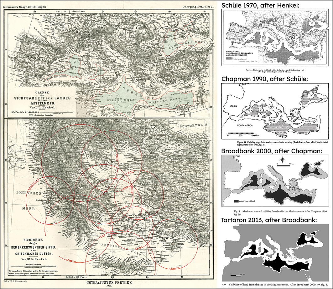
For half a century, archaeologists interested in maritime navigation in the Mediterranean Sea have turned to Wilhelm Schüle’s map of “Grenze der Sichtbarkeit des Landes auf dem Mittelmeer” (“limit of visibility of land in the Mediterranean”; Schüle Reference Schüle1970: fig. 1, Reference Schüle1980: fig. 2). Although Schüle is credited in these publications as the originator of this map, it is in fact a duplicate of a 1901 analysis of Mediterranean and Aegean visibility by Ludwig Henkel (Reference Henkel1901: fig. 1; see Figure 1). Schüle introduced Henkel’s map and formula to archaeology first in a conference paper and later in the preface to a site monograph (Schüle Reference Schüle1970, Reference Schüle1980), describing his own map as a ‘slightly simplified reproduction’ of Henkel’s. Since Schüle uses the same formula, references identical source data and replicates Henkel’s anachronistic treatment of the Nile Delta (see below), we consider his map to be a direct copy of Henkel’s (cf. Schüle Reference Schüle1970: 458–60; Henkel Reference Henkel1901: 285; see also Table 1).

Figure 1.

Henkel’s map of Mediterranean visibility/isovists for selected mountain peaks in the Aegean (left; 1901: fig. 1), and selected reproductions of Henkel’s map (right) (figure by Karl Smith; © The Practical Mariner).

Table 1.

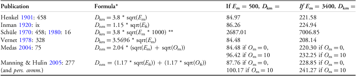
Published isovist formulae.

*D _units = visible distance; E _units = land elevation; O _units = observer height; nm = nautical miles.

**Schüle’s addition of the ‘1000’ term likely resulted from confusion over unit conversions. His example “11.4 = 3.8* sqrt(9 * 1000)” (1980: 16) is only correct if the ‘1000’ term is removed, in which case the formula is identical to Henkel’s.

Critical examination of the use of Henkel’s map in archaeological analyses reveals how it has been used to support different ‘expansive’ models of maritime mobility—that is, models in which long-distance voyages were regular, frequent and/or easily accomplished. Henkel’s original formulation was itself inspired by a curiously anthropomorphic view of prehistoric seafaring. In the introduction, Henkel (Reference Henkel1901: 284) cites as his inspiration Neumann and Partsch’s Geographie von Grieschenland, which he claimed contained “perhaps the most beautiful” description of the use of landmarks in ancient navigation:

Henkel uses similar framing in claiming that his map shows how “the Carthaginian sailor never lost sight of land on his voyages to Sardinia or Sicily, as the islands of Galite and Pantellaria guided him across” (Reference Henkel1901: 284–85; authors’ translation). For these authors, the long-distance visibility of landforms enabled—perhaps even motivated—prehistoric voyages.

Schüle, meanwhile, approached maritime mobility mainly as a mechanism to explain the movement of archaeological material around Mediterranean shores, arguing that similarities between artefacts in areas connected by the sea suggested direct, long-distance contact (see citations in Schüle Reference Schüle1980: 17). While contemporary scholars, such as Bowen (Reference Bowen and Moore1970), used distribution maps to support their maritime theories, Schüle turned to Henkel’s visibility map:

Arguments similar to Schüle’s have been voiced more recently by Aubet (Reference Aubet2001: 168), who supports her argument that Phoenicians must have made long-distance overnight voyages by claiming (audaciously) that “it has been proved that in favourable weather conditions, with very few exceptions, the coast or the mainland is visible from any point in the Mediterranean” in reference to Schüle’s map. Tartaron (Reference Tartaron2013: 108–109) also uses Henkel’s map in support of an argument that long-distance offshore navigation was possible throughout the Mediterranean, except between Crete and Libya. Other authors use Henkel’s map to suggest areas that navigators may have preferred or avoided, without arguing that the map supports a particular theory of Mediterranean mobility (Chapman Reference Chapman1990: fig. 59; Cunliffe Reference Cunliffe2008: fig. 212, Reference Cunliffe2017: fig. 2.4; Calvo-Trias & Galmés-Alba Reference Calvo-Trias and Galmés-Alba2025: fig. 1). The remaining appearances of Henkel’s map in archaeological literature use it to provide general context for their maps of the Mediterranean (Broodbank Reference Broodbank2000: fig. 4, Reference Broodbank2015: overleaf; Horden & Purcell Reference Horden and Purcell2000: fig. 9; Höckmann Reference Höckmann and Yalçin2005: fig. 1).

Unfortunately, most archaeological reproductions of Henkel’s map are confused about or indifferent to its provenance. Many of the aforementioned works do not cite any source for the map, or else cite a source other than Henkel or Schüle. For example, Tartaron’s (Reference Tartaron2013) version of Henkel’s map is attributed to Broodbank (Reference Broodbank2000), who attributes it to Chapman (Reference Chapman1990), who attributes it to Schüle (Reference Schüle1980) (see Figure 1). This confusion is probably one of the reasons why Henkel’s ‘visibility limit’ has escaped criticism despite its widespread use in archaeological analyses. None of these cited authors have attempted to evaluate Henkel’s method on its own terms—as a spatial analysis—or presented arguments for or against its application to archaeological problems.

Evaluating Henkel’s ‘visibility limit’

Henkel’s map is based on a simple formula: the distance (in kilometres) within which a point on land should be visible is equal to 3.8 multiplied by the square root of the point’s elevation (in metres; see Table 1). Henkel produced his map by applying this formula to 62 mountain peaks spread throughout the Mediterranean littoral (Henkel Reference Henkel1901: 285). This method can be described in modern GIS terms as merging 2D buffers to create a visibility isoline, or ‘isovist’ (see Benedikt Reference Benedikt1979; Lonergan & Hedley Reference Lonergan and Hedley2016). Unlike architectural isovists, which show the theoretical limits of visibility from a particular point, Henkel’s formula produces an isoline that represents the limits of visibility of a set of points. However, Henkel did not apply his formula consistently; for the Nile Delta, he replaced his isoline with a 20-nautical-mile buffer (representing the visible distance of lighthouses), because “otherwise [the visibility limit] would run close to the flat shore” (Henkel Reference Henkel1901: 285; authors’ translation). He also did not provide a source for his formula in his 1901 paper but did express hope that it would “stimulate observations [of] the extent to which practical visibility corresponds to theoretical visibility” (Henkel Reference Henkel1901: 285; authors’ translation).

Henkel’s formula is one of several similar formulae published by archaeologists (compared in Table 1). McGrail (Reference McGrail1998) published an isovist formula in 1987, which he attributes to the 1920 edition of Inman’s Nautical tables (Inman Reference Inman1920, ix). McGrail (Reference McGrail1998: 278) describes this formula as an “approximation [of] theoretical distances from sea-level”, noting that “in meteorological conditions of refraction high ground may be seen at more than the theoretical distance. In poor visibility the distance is much less”. Vernet (Reference Vernet1978: 328) independently derived his own visible-distance formula, which includes a variable for observer elevation above sea level. Vernet’s paper is probably the source or inspiration for Medas’s (Reference Medas2004: 75) isovist formula, applied to Mount Etna (Medas cites Schüle, McGrail and Vernet; but Table 1 shows his results agree with Vernet). Medas’s formula has been used recently in visibility analyses by Calvo-Trias and Galmés-Alba (Reference Calvo-Trias and Galmés-Alba2025: 272–74), which include isovists as a component in GIS visibility analyses of the Baleares. A final isovist formula was independently developed by Manning and Hulin (Reference Manning, Hulin, Blake and Knapp2005: fig. 1), whose equation also takes observer height into account. Their map of visibility in the Eastern Mediterranean is reproduced by Cunliffe (Reference Cunliffe2017: fig. 3.9), with the visibility limit blurred so as not to suggest a hard cutoff.

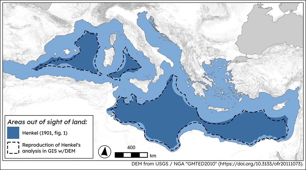
Publications that cite Henkel or Schüle do not critique Henkel’s method, input data or results, and typically focus on regions of the Mediterranean rather than the entire basin. We therefore provide an evaluation of Henkel’s data sources and method—specifically, his reliance on isovists based on a small set of mountain peaks (and lighthouses)—by reproducing his map in GIS. We based our reproduction on Henkel’s formula and the GMTED2010 global 15-arcsecond digital elevation model (DEM; see Danielson & Gesch Reference Danielson and Gesch2011). For each cell in the DEM, we constructed a buffer in ESRI ArcGIS Pro 3.6 using Henkel’s formula and merged these buffers to generate the isovist shown in Figure 2.

Figure 2.

Map comparing Henkel’s Reference Henkel1901 isovist (dark blue) with our GIS reproduction (dashed line) (figure by Karl Smith; © The Practical Mariner).

Initially, our isovist appears to be similar to Henkel’s. At a Mediterranean-wide scale it is slightly more conservative: the total ‘out of sight of land’ area defined by our model is approximately 1.6 per cent larger than Henkel predicts. However, focusing on specific areas reveals larger discrepancies. For example, we have not reproduced Henkel’s decision to base his isovist on lighthouses rather than mountain peaks in the Nile Delta. As such, the distance between ours and Henkel’s isovist is approximately 20–40km in the delta, with our results suggesting (as Henkel suspected) that the delta would have been visible only within 5–10km of the shore. There are also large distances between ours and Henkel’s isolines in the Black Sea, off the west coast of Greece, the north coast of the Italian island of Ustica, the east coast of Sardinia and the south coasts of Cyprus and the Baleares. In all cases the furthest distance between the two isolines is 35–50km. On the other hand, both models confirm Henkel’s (Reference Henkel1901: 258) assertion that land ought to be visible from anywhere within the Aegean and Adriatic. Additionally, both models suggest that it is possible to maintain sight of land while sailing between the Baleares and the mainland, between Sardinia and Africa, and between Cyprus and the Levant.

These comparisons illustrate how the application of Henkel’s method can be improved by using all cells in a DEM rather than a small number of topographic prominences/lighthouses. We can also critique isovist formulae on a theoretical level by comparing them directly. Table 1 demonstrates that, because published isovist formulae have exponential terms, plotting the results of these functions for a range of land elevations results in a set of curves that grow further apart as elevation increases. For example, the difference between the greatest and least ‘visible distance’ values produced by these formulae for a point 500m high is 1.78km, but the same difference for a point the height of Mount Etna (approx. 3400m) is 20.72km. The same effect technically applies to the observer-height terms in Medas’s and Manning and Hulin’s formulae, but the smaller range in plausible viewing elevations makes the difference negligible. To the best of our knowledge, these observations constitute the only published comparative analysis of these isovist formulae. We believe that these theoretical methods should be confirmed by experiment (in the field or in GIS) before isovist formulae are accepted as valid methods for estimating the visibility of land.

Considering viewshed-based approaches to maritime visibility

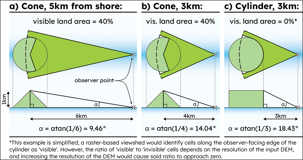
The most obvious GIS alternative to an isovist-based approach to the maritime visibility of land would be a viewshed-based approach. The viewshed algorithm is a widely used GIS technique for quantifying visibility (for example: Wheatley & Gillings Reference Wheatley, Gillings and Lock2000; Llobera Reference Llobera2003; Brughmans et al. Reference Brughmans2018), which tests observer-target sight lines against a raster elevation surface—if a sightline is obstructed the cell is marked as ‘not visible’, and if it is unobstructed the cell is marked as ‘visible’ (see Fisher Reference Fisher1993). Viewsheds can be combined to create ‘cumulative’ visibility analyses (in the context of seafaring, see Gillings Reference Gillings2009; Gustas & Supernaut Reference Gustas and Supernant2017; Calvo-Trias & Galmés-Alba Reference Calvo-Trias and Galmés-Alba2025). The only direct archaeological critique of Henkel’s map (or, more precisely, of Aubet’s Reference Aubet2001 reproduction) is Čučković’s (Reference Čučković2016, Reference Čučković2018) cumulative viewshed analysis for the Mediterranean using the Quantum GIS plug-in for QGIS. In his analysis, the value in each cell of the image represents the results of a viewshed with an observer in that cell. Čučković used 50km and 150km distance-bands to simulate visibility under different conditions, and it is telling that these bands are parameters, not products, of his model. This is necessary because viewsheds are designed primarily to quantify obstruction—the results of a single viewshed are not sensitive to changes in the relative positions of observer and target, except insofar as that change in position increases or reduces the target features’ visible area. To illustrate why this distinction is especially important in a maritime setting, consider the following hypothetical situations (illustrated in Figure 3).

Figure 3.

A comparison of the results of viewshed (in plan, top) and angular visibility measurement (in section, bottom) on idealised landforms seen from the sea (figure by Karl Smith; © The Practical Mariner).

Imagine you are floating in the sea 5km off the shore of a small island. The island is conical, has a diameter of 2km and rises 1km above sea level. In this scenario the sea is a flat plane, so the angle between your horizon and the highest visible point of the island can be calculated by taking the arctangent of the island’s elevation divided by the distance from the observer to the island’s centre—in this case 0.165 radians or 9.45° (Figure 3a). On the other hand, if the island is perfectly conical a viewshed will tell you that about 40 per cent of the cone’s area is visible. Now sail 2km towards the island and go for another swim. Using the arctangent formula, you calculate that the island’s angle-above-horizon increases from 9.45° to 14.04° (Figure 3b). Meanwhile, at a distance of 3km our perfectly conical island will remain 40 per cent visible according to the viewshed. Finally, imagine that the island is cylindrical instead of conical (Figure 3c; in a more realistic scenario it might be surrounded by cliffs). From your vantage point 3km off the shore the island’s angle-above-horizon increases to 18.43°, because the upper rim of the cylinder is closer to you than the island’s centre. But because the edge of the cylinder now obstructs your view of the top of the island, the island’s ‘visible area’, according to a viewshed, drops from 40 per cent to a negligible percentage (for details, see Figure 3c).

These thought experiments illustrate two important points. First, ‘visible area’ defined by a viewshed does not necessarily increase or decrease as an observer moves towards or away from the target, provided that the target is regularly-shaped and there are no intervening obstacles. Second, viewsheds will fail to recognise as ‘visible’ features defined by cliffs when an observer is at the cliff base. In both cases, using angular measures fits our basic assumptions about visibility (land should be more visible when closer; larger landforms should be more visible than smaller landforms), while measurements of visible area produce counterintuitive results. These limitations have been highlighted in terrestrial viewshed applications (i.e. Wheatley & Gillings Reference Wheatley, Gillings and Lock2000: 25), but in a maritime context they are much more difficult to excuse.

Building a 3D visibility model

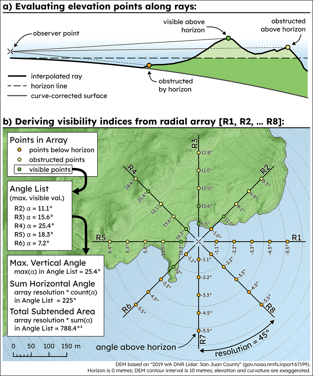
Given the limitations of the isovist and viewshed approaches to the visibility of land from the sea, we developed a 3D GIS method for measuring the visibility of land in angular terms using Python and ESRI ArcGIS geoprocessing tools. This technique follows 3D approaches to landscape and ‘coastscape’ assessment (especially: Higuchi Reference Higuchi1983; Jerpåsen Reference Jerpåsen2009; Bernardini et al. Reference Bernardini2013). Following Pouncett (Reference Pouncett2013), our scripts generate a radial array centred on an observer point, sampling points on that array to compute visibility indices (see Figure 4). We then generate a list of points at regular intervals along each ray, and adjust the elevation-values of these points to simulate Earth curvature (see Yoeli Reference Yoeli1985: 92–93). Next, we check that these points are (1) unobstructed by other points along the ray, and (2) within a pre-set maximum visible distance. Upon completing this check, our script returns either an empty list (in which case no points along the ray are visible), or a list of visible elevations. Finally, we compute angular values for all visible elevation points using the arccosine function.

Figure 4.

Illustration of the radial array method with elevation and curvature exaggerated, showing: a) curvature-correction and obstruction-checking for individual rays, and b) calculation of visibility indices for a simple array (figure by Karl Smith; © The Practical Mariner).

Using these lists, our scripts compute three angular visibility indices: maximum vertical angle, sum horizontal angle and total subtended area. These represent, respectively, the highest angle that land appears at over the horizon, the angle along the horizon occupied by land and the ‘size’ of land as it appears to a viewer. Maximum vertical angles are calculated by finding the maximum angular value for all rays in the radial array. To compute the sum horizontal angle, our script multiplies the number of rays that return visible elevations by the angular resolution of the array. Finally, total subtended area is calculated by finding the maximum angular value for each ray in the array and multiplying the sum of these values by the array’s angular resolution.

Our other scripts co-ordinate our visibility model over the following dimensions: latitude, longitude, sea level height and maximum visible distance. In the first two cases, every combination of latitude and longitude are tested for intersection with features representing land to obtain a regular grid of 2D points that are located at sea. A radial array is constructed for each point, and the process described above is completed for (1) a series of observer heights, and (2) a series of maximum visible distances. The final output of our script is a 5D array, stored as a NetCDF file (see Rew & Davis Reference Rew and Davis1990). NetCDF is a flexible data format that stores variables (in our case: maximum vertical angle, sum horizontal angle and subtended area) at points along a set of dimensions (for us: x-coordinate, y-coordinate, water surface height, observer height and maximum visible distance). Using GIS/statistics software our 5D arrays can be queried to determine, for example, visibility values for certain points, or sliced/flattened to produce raster images. The figures presented in this article are subsets of our larger visibility arrays (see OSM).

A new Mediterranean maritime visibility map

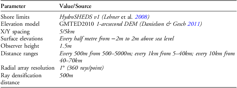
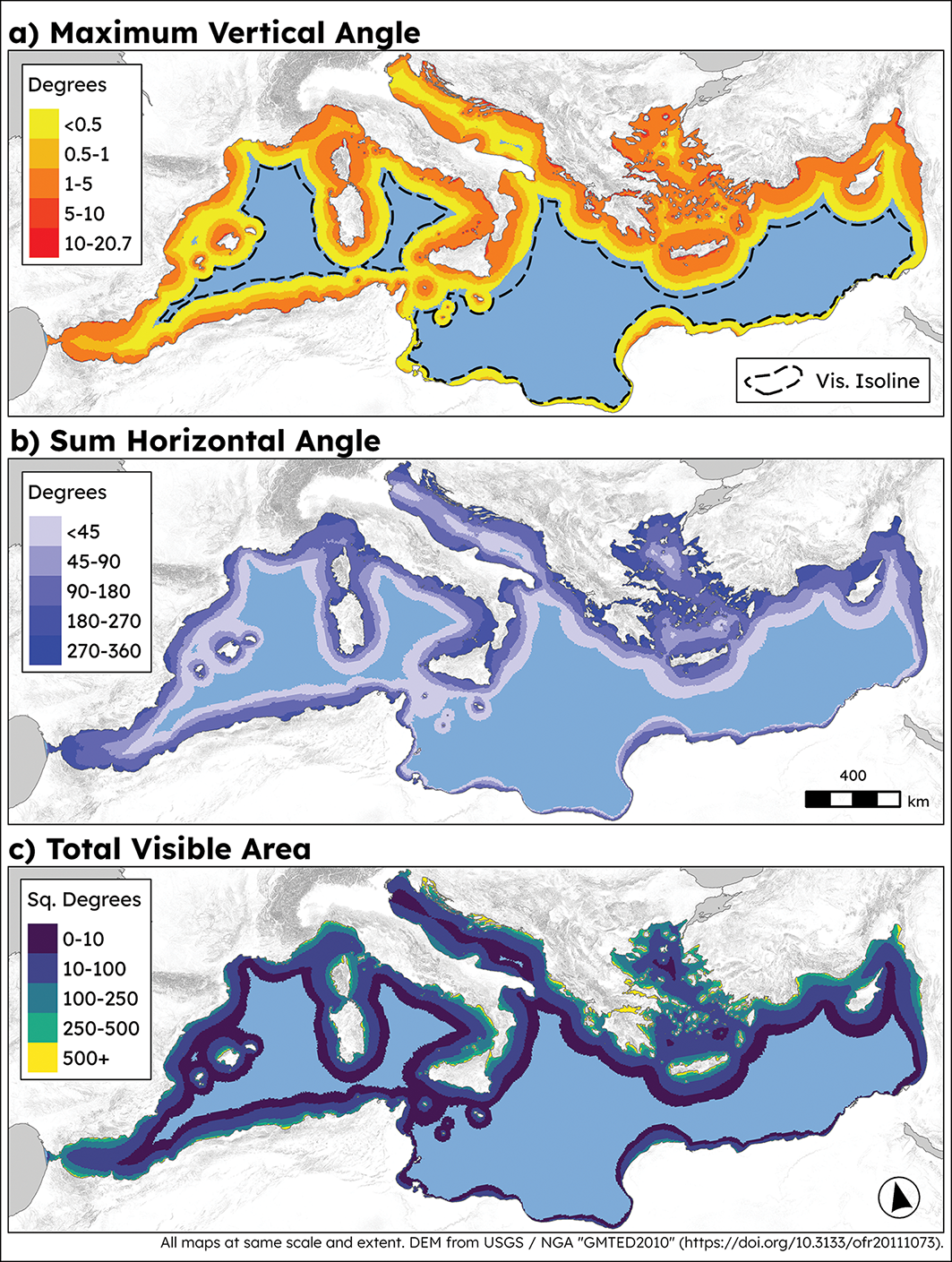
We used our projective visibility scripts to perform an analysis for the Mediterranean for a 5km grid of points masked by the HydroSHEDS v.1 hydrological dataset (see Lehner et al. Reference Lehner2008). We used four tide heights, an observer height of 1.5m and a range of visible distances corresponding to weather types reported by the World Meteorological Organization (2009: A-351). Other variables used by the script and in our analysis can be found in Table 2. We imported the resulting NetCDF file into ArcGIS Pro and extracted data slices as rasters to create the figures in this article. Figure 5 shows angular measures derived from our model’s output, classified into categories. Figure 5a shows that the outer limit of visibility defined by our model is broadly similar to our isovist. There are, however, some important discrepancies: our model contains areas ‘out of sight of land’ within the Adriatic and between Cyprus, the Baleares and their respective mainlands, and does not suggest that maintaining sight of land while sailing between Sardinia and Africa is possible. The values in Figure 5a are much lower than expected, only rising higher than 5° within 5–20km of the coast in most cases. The classified sum horizontal angle plot (Figure 5b) highlights ‘enclosed’ areas, where seafarers would have been able to see more land along the horizon—especially the Cyclades, Anatolia, the Dalmatian Coast and the straits of Gibraltar and Messina. In the case of Cyprus, it suggests that sailors approaching from the north would have stood the best chance of keeping land in view along the horizon. Finally, the classified total subtended area plot (Figure 5c) is a useful synthesis of the two other indices. It highlights visually prominent coastlines like that of Crete and Sicily, as well as littoral areas that are relatively more visible, like the eastern Libyan coast.

Table 2.

Parameter inputs and data sources for our visibility model.

Figure 5.

Classified results of the Mediterranean visibility model (figure by Karl Smith; © The Practical Mariner).

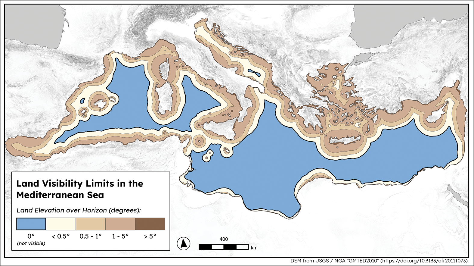
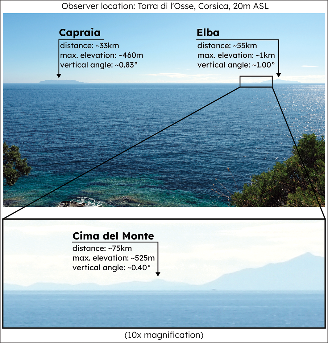
We believe that of the three measures, the maximum vertical angle is the most directly comparable to isovist results and is also the easiest to understand intuitively. We therefore use this measure as the basis for our updated Mediterranean visibility map (Figure 6). To produce this map, we ran the ArcGIS ‘Contour’ tool on a slice of our unclassified maximum vertical angle dataset (for parameters used to define the slice, see the readme file in the OSM). The contours in this case represent the areas in which land can be seen at 0, 0.5, 1 and 5+° above the horizon. While the outer limits of visibility in our map are broadly similar to Henkel’s, there is considerable variability within that outer limit. For example, our analysis suggests crossings from the Balkans to Italy, from Sicily to Africa, across the Gulf of Lion and from the Baleares to Europe would have involved traversing areas of the sea where land rises less than half a degree above the horizon. In fact, our models suggest that for most of the area within Schüle’s ‘visibility limit’, land rises less than half a degree above the horizon. For reference, the width of your smallest finger held at arm’s length is approximately one degree; Figure 7 shows three landforms that rise up to one degree above the horizon (as calculated by our Python scripts), viewed under good conditions. We believe that mariners without telescopes or night-glasses would find it difficult to identify landforms that rise less than half a degree above the horizon—especially in foul weather—even if land technically could be viewed.

Figure 6.

An updated visibility map for the Mediterranean (figure by Karl Smith; © The Practical Mariner).

Figure 7.

Maximum vertical angle measurements calculated for peaks on the islands of Capraia and Elba, viewed from Corsica, with magnified inset at bottom showing the same measurements for Cime del Monte, Elba (figure by Karl Smith; © The Practical Mariner).