


1. Introduction
Thermoacoustic instabilities are a persistent challenge in the design of combustion systems, particularly modern low-emission gas turbine combustors. They arise from a positive feedback loop between acoustic waves and heat release fluctuations (Culick Reference Culick2006). The acoustic waves perturb the flame, generating heat release fluctuations. If the heat release fluctuations are sufficiently in phase with the acoustic pressure, they add energy to the acoustic field and the amplitude of oscillations grows.
Thermoacoustic instabilities are difficult to predict because they are extremely sensitive to small changes in a system's design or operating conditions (Juniper & Sujith Reference Juniper and Sujith2018). From a designer's perspective, this can be beneficial because small design changes can be used to stabilize a design. The challenge lies, however, in identifying the appropriate changes (Mongia et al. Reference Mongia, Held, Hsiao and Pandalai2003). The sensitivity of thermoacoustic behaviour makes it difficult to develop quantitatively accurate models, because the model predictions are sensitive to small changes in the values of unknown model parameters. This has been a persistent challenge, because models could be carefully tuned to match experimental data at one operating condition, but fail to match the data at nearby operating conditions (Matveev Reference Matveev2003).
The modeller can, however, exploit this extreme sensitivity if a data-driven modelling approach is taken. This is because the sensitivity makes the uncertain model parameters easy to observe from experimental data. With carefully planned experiments, it is possible to (i) infer the unknown parameters of a physics-based model, (ii) rank several candidate models and select the best one (Juniper & Yoko Reference Juniper and Yoko2022) and (iii) determine whether more data are required, and identify which experiments to perform to collect those data (Yoko & Juniper Reference Yoko and Juniper2023).
Using this approach, we have previously constructed a model of a hot-wire Rijke tube that is quantitatively accurate over a wide operating range (Juniper & Yoko Reference Juniper and Yoko2022), despite containing few parameters. A subsequent study on the same system applied Bayesian experimental design to identify the most informative experiments, allowing us to infer the model parameters using fewer experimental observations (Yoko & Juniper Reference Yoko and Juniper2023). In this paper we apply this data-driven modelling framework to thermoacoustic oscillations of a ducted conical flame.
The fluctuating heat release rate of a flame is typically modelled as a response to a velocity perturbation at some reference location near the base of the flame. A commonly used model is the flame transfer function
 \begin{equation} \mathcal{F} = \frac{Q'/\bar{Q}}{u'/\bar{u}}, \end{equation}
where  $\mathcal {F}$ is the (frequency-dependent) flame transfer function, $Q$ is the heat release rate and $u$ is the velocity at a reference location near the base of the flame. The fluctuating quantities are denoted as $\star '$ and mean quantities are denoted as $\bar {\star }$.
The flame transfer function has been shown to change sensitively with changes in the operating condition (Gatti et al. Reference Gatti, Gaudron, Mirat, Zimmer and Schuller2018; Nygård & Worth Reference Nygård and Worth2021), changes to the confinement of the flame (Cuquel, Durox & Schuller Reference Cuquel, Durox and Schuller2013b; Tay-Wo-Chong & Polifke Reference Tay-Wo-Chong and Polifke2013) and when the flame is combined with other flames (Durox et al. Reference Durox, Schuller, Noiray and Candel2009; Æsøy et al. Reference Æsøy, Indlekofer, Gant, Cuquel, Bothien and Dawson2022). It is therefore beneficial to determine the flame transfer function with the flame in situ.
The flame transfer function is typically obtained from direct experimental measurements. These measurements require (i) a means of measuring acoustic velocity at the reference location near the base of the flame, and (ii) a means of measuring the heat release rate fluctuations. The velocity is typically measured using a hot-wire anemometer (Kornilov, Schreel & De Goey Reference Kornilov, Schreel and De Goey2007; Mejia, Miguel-Brebion & Selle Reference Mejia, Miguel-Brebion and Selle2016; Gatti et al. Reference Gatti, Gaudron, Mirat, Zimmer and Schuller2018) or via optical methods (Ducruix, Durox & Candel Reference Ducruix, Durox and Candel2000; Birbaud, Durox & Candel Reference Birbaud, Durox and Candel2006; Cuquel, Durox & Schuller Reference Cuquel, Durox and Schuller2013a). The heat release rate fluctuations are typically measured by optical methods (Ducruix et al. Reference Ducruix, Durox and Candel2000; Birbaud et al. Reference Birbaud, Durox and Candel2006; Kornilov et al. Reference Kornilov, Schreel and De Goey2007; Cuquel et al. Reference Cuquel, Durox and Schuller2013a; Mejia et al. Reference Mejia, Miguel-Brebion and Selle2016; Gatti et al. Reference Gatti, Gaudron, Mirat, Zimmer and Schuller2018). None of these measurement techniques are suitable for in situ measurements in a practical combustor, because they either rely on delicate instruments being mounted in a harsh operating environment, or on optical access, which is typically limited or unavailable in a practical combustor. By contrast, it is relatively easy to measure the acoustic pressure fluctuations in a practical combustor. It is therefore valuable to be able to infer the fluctuating heat release rate parameters from pressure measurements alone.
Recent work in the Rolls-Royce SCARLET thermoacoustic test rig has demonstrated a method for obtaining the flame transfer function directly from pressure measurements (Fischer & Lahiri Reference Fischer and Lahiri2021; Treleaven et al. Reference Treleaven, Fischer, Lahiri, Staufer, Garmory and Page2021) using the two-source method (Munjal & Doige Reference Munjal and Doige1990; Paschereit et al. Reference Paschereit, Schuermans, Polifke and Mattson1999). This method uses acoustic pressure measurements from multiple microphones, collected from four experiments. In the first two experiments, the cold rig is forced harmonically at various frequencies from the upstream end and then the downstream end. In the next two experiments the flame is ignited, and the rig is again forced at the same frequencies from the upstream end and then the downstream end. The resulting data are then post-processed to extract (i) the characteristics of the cold rig, and (ii) the flame transfer function. This demonstrates a method for obtaining flame transfer functions from pressure measurements, but does not yet quantify the uncertainty in the measurements or the inferred quantities.
To measure the growth rate indirectly, Noiray (Reference Noiray2017) and Noiray & Denisov (Reference Noiray and Denisov2017) applied system identification to infer the parameters of a stochastic differential equation describing the amplitude of thermoacoustic oscillations. This approach can infer linear growth rates from limit cycle data, which are simpler to collect than forced data. However, the inference framework used does not consider the uncertainty in the inferred quantities. Furthermore, this method gives the growth rate of oscillations, rather than model the thermoacoustic system itself.
A few recent studies have applied data-driven methods to infer the parameters of a fluctuating heat release rate model from pressure time series data (Ghani, Boxx & Noren Reference Ghani, Boxx and Noren2020; Gant et al. Reference Gant, Ghirardo, Cuquel and Bothien2022; Ghani & Albayrak Reference Ghani and Albayrak2023). In the work of Ghani et al. (Reference Ghani, Boxx and Noren2020) and Ghani & Albayrak (Reference Ghani and Albayrak2023), a non-probabilistic approach is used to infer the parameters. The authors use an optimization algorithm to minimize the discrepancy between the model and data, although they do not consider the uncertainties, or the resulting uncertainties in the inferred parameters. In the work of Gant et al. (Reference Gant, Ghirardo, Cuquel and Bothien2022), a frequentist approach is used to infer the fluctuating heat release rate from pressure time series data. In the frequentist framework, the authors are able to quantify the uncertainty in the inferred parameters. They cannot, however, exploit prior knowledge or evaluate the marginal likelihood in order to compare candidate models. Gant et al. (Reference Gant, Ghirardo, Cuquel and Bothien2022) demonstrate their method on synthetic data generated by their model. While this is a powerful tool for evaluating and demonstrating an inference framework, it does not allow the researcher to evaluate how the method handles a systematic mismatch between the model and the data, which is always present when assimilating experimental data into a model.
In this paper, we apply adjoint-accelerated Bayesian inference to infer the flame transfer functions of a series of conical flames from pressure observations. We use Bayesian model comparison to choose the best model for the fluctuating heat release rate from a set of candidate models. We then infer the most probable flame transfer function for each flame, and rigorously quantify the uncertainties in each of the flame transfer functions. In its broader forms, Bayesian inference has been applied in astronomy and astrophysics (Jenkins & Peacock Reference Jenkins and Peacock2011; Thrane & Talbot Reference Thrane and Talbot2019; Agazie et al. Reference Agazie2023; Antoniadis et al. Reference Antoniadis2023), biology (Huelsenbeck et al. Reference Huelsenbeck, Ronquist, Nielsen and Bollback2001; Wilkinson Reference Wilkinson2007; Chowdhary, Zhang & Liu Reference Chowdhary, Zhang and Liu2009), economics (Harvey & Zhou Reference Harvey and Zhou1990; Flury & Shephard Reference Flury and Shephard2011; Lux Reference Lux2023), geophysics and meteorology (Nabney, Cornford & Williams Reference Nabney, Cornford and Williams2000; Isaac et al. Reference Isaac, Petra, Stadler and Ghattas2015; Epstein Reference Epstein2016; Wang et al. Reference Wang, Maeda, Satake, Heidarzadeh, Su, Sheehan and Gusman2019) and engineering, where it has predominantly been applied in structural mechanics (Karandikar, Kim & Schmitz Reference Karandikar, Kim and Schmitz2012; Rappel et al. Reference Rappel, Beex, Hale, Noels and Bordas2020; Ni et al. Reference Ni, Han, Du and Cheng2022).
By comparison, engineers working in fluid dynamics have made little use of the Bayesian framework. In their review of machine learning in fluid dynamics, Brunton, Noack & Koumoutsakos (Reference Brunton, Noack and Koumoutsakos2020) argue that, for fluid mechanics problems, Bayesian inference may be superior to other machine learning techniques because of its robustness, but that it is hampered by the cost of the thousands of model evaluations required to compute the posterior distribution. While this is true of typical sampling methods, such as Markov chain Monte Carlo (MCMC), it is not true of the inference framework we demonstrate in this paper. This framework reduces the required model evaluations, making Bayesian inference feasible for computationally expensive models (Isaac et al. Reference Isaac, Petra, Stadler and Ghattas2015; Kontogiannis et al. Reference Kontogiannis, Elgersma, Sederman and Juniper2022).
2. Experimental configuration
The experimental set-up is a laminar premixed conical flame inserted into a vertical duct, illustrated in figure 1. The lower end of the duct is fixed to a plenum chamber, through which co-flow air is supplied. The upper end is open to the atmosphere.
Diagram of the experimental rig.

The duct is a 0.8 m long section of quartz tube with an internal diameter of 75 mm. The duct joins the plenum via a machined flange. The flange provides an airtight seal and an acoustic termination without any internal steps. Eight holes have been drilled along the length of the duct to allow for instrument access to the internal flow.
The plenum is a fibreboard box with dimensions  $1\ {\rm m}\times 0.6\ {\rm m} \times 0.6\ {\rm m}$. The interior is lined with acoustic treatment to damp acoustic oscillations. Air is fed into the plenum via a mass flow controller to provide a constant flow of cool air through the duct. This keeps the duct and instrumentation at an acceptable temperature, and flushes the combustion products out of the rig.
The burner is a 0.85 m long section of brass tubing with an internal diameter of 14 mm. The outlet of the burner is fitted with a nozzle that is chosen such that the system can become thermoacoustically unstable. At the injection plane, the nozzle diameter is 9.35 mm. The burner is fuelled by a mixture of methane and ethylene. This mixture allows a wide range of thermoacoustic behaviour to be explored by altering the shape of the flame by changing the unstretched flame speed. The premixed air and fuel are supplied to the base of the burner via a set of mass flow controllers. The base of the burner is fitted with a choke-plate to decouple the supply lines from the acoustic fluctuations in the rig. Like the duct, the burner tube has eight ports for instrument access to the internal flow.
The burner is mounted to an electrically driven traverse so that the vertical position of the burner inside the duct can be controlled. We are therefore able to explore changes in (i) flame position, (ii) flame shape (through changes in fuel composition) and (iii) mean heat release rate (through total fuel flow rate and fuel composition).
The rig is instrumented with eight probe microphones, which provide point measurements of the acoustic pressure. Seven of the probe microphones are fitted through the ports in the duct, with the probes placed near the inner wall. The eighth microphone is fitted through a port near the base of the burner. We also collect data from 24 fast response thermocouples. Eight K-type thermocouples are installed within the plenum to monitor the ambient conditions, another eight are inserted through ports in the duct to monitor the internal gas temperature and the final eight are bonded to the duct's outer wall to monitor the duct temperature. The data acquisition and control of the rig have been automated so that we can cheaply collect a large amount of data.
When the system is linearly stable, a loudspeaker mounted within the plenum is used to force the system harmonically near its fundamental frequency. The forcing is sustained for six seconds and then terminated, following which the oscillations decay to zero. We record data during a 15 second window beginning with the onset of forcing. When the system exhibits self-excited oscillations, we stabilize the system using active feedback control with a phase-shift amplifier. We begin recording data while the stabilization is active, then deactivate the stabilization and allow the oscillations to grow to a limit cycle. Each experiment is repeated 75 times so that we can estimate the random uncertainty in the experimental data. We also considered the uncertainty due to the precision of the measurement chain, but found this to be negligible compared with the random uncertainty.
We process the raw pressure signals to extract (i) the growth or decay rate, (ii) the natural frequency and (iii) the Fourier-decomposed pressure of seven of the microphones, which we measure relative to the eighth (reference) microphone. This forms our experimental observations for inference, which we collectively refer to as the observation vector,  $\boldsymbol {z}$. The observed variables are all complex numbers, but are stored in real–imaginary form such that the observation vector is a real vector.
We investigate 24 different flames, which are selected to explore a wide range of thermoacoustic behaviour. We parameterize the flames based on (i) the convective time delay,  $\tau _c = L_f/\bar {U}$, which is the time taken for a perturbation travelling at the bulk velocity, $\bar {U}$, to travel along the length of the flame, $L_f$, and (ii) the mean heat release rate of the inner cone, $\bar {Q}$.
We split the 24 flames into six groups of four flames, and select the composition of each flame such that the convective time delay is constant within each group and the mean heat release rate varies. The convective time delays range from 9.5 to 17 ms in 1.5 ms increments, and the mean heat release rates range from 375 to 600 W in 50 W increments. These flames produce thermoacoustic behaviour ranging from strongly damped, to neutral to strongly driven.
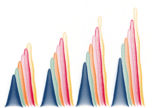
We calculate the flow rates required to achieve the desired convective time delays and heat release rates using Cantera (Goodwin et al. Reference Goodwin, Moffat, Schoegl, Speth and Weber2022) and a simple linear model for a steady conical flame. The linear model over-predicts the flame lengths, and therefore the convective time delays, because it neglects the effect of curvature on the laminar flame speed. We therefore verify the actual convective time delays experimentally by measuring the length of the steady flames from flame images. The flame properties are summarized in table 1, and the flames are illustrated in figure 2.
Summary of the properties of the 24 flames studied. We show the average measured flow rates of air, methane ( $\mathrm {CH_4}$) and ethylene ( $\mathrm {C2H_4}$), the equivalence ratio ( $\phi$), the bulk velocity in the burner tube ( $\bar {U}$), the predicted and measured flame lengths ( $L_f$), the predicted and measured convective time delays ( $\tau _c$) and the inner cone mean heat release rate ( $\bar {Q}$).

Processed steady flame images from the 24 flames. Images are grouped and artificially coloured according to their approximate convective time delay,  $\tau _c$. Each convective time delay is studied at four mean heat release rates, $\bar {Q}$. Flames with low mean heat release rate are shown in darker shades and flames with high mean heat release rate are shown in lighter shades.

3. Physics-based model of a ducted flame
We assimilate the data into a travelling-wave network model, modified from a previous study (Juniper & Yoko Reference Juniper and Yoko2022) to handle multiple coupled acoustic networks. The model predicts the growth rate,  $s_r$, angular frequency, $s_i$, and acoustic pressure, $P$, which we collectively refer to as the prediction vector, $\boldsymbol {s}$. The model is shown schematically in figure 3.
Diagram of the acoustic network model used in this study. The unknown model parameters are:  $R_\star$, the reflection coefficients at the boundaries, $\eta _\star$, the strengths of the visco-thermal damping and $\mathcal {F}$, the transfer function from velocity perturbations to heat release rate fluctuations.

The model contains several parameters, the values of which we do not know a priori. These parameters arise from the modelling of (i) the reflection/transmission of acoustic energy at the ends of the duct and at the base of the burner, (ii) the visco-thermal damping in the boundary layer on the duct and burner walls and (iii) the fluctuating heat release of the flame.
We model item (i) using complex reflection coefficients which we label  $R_u$, $R_d$ and $R_b$ for the upstream and downstream ends of the duct and the base of the burner, respectively. Items (ii) and (iii) are modelled using local linear feedback from acoustic pressure or velocity into the energy or momentum equations (Chu Reference Chu1965; Juniper Reference Juniper2018), which we label $k_{eu}$, $k_{ep}$, $k_{mu}$ and $k_{mp}$.
The linear feedback coefficients can either be inferred directly, or calculated using analytical models. For example, models have been proposed for the reflection coefficient at the open end of a flanged (Zorumski Reference Zorumski1973; Norris & Sheng Reference Norris and Sheng1989) and unflanged (Levine & Schwinger Reference Levine and Schwinger1948; Selamet, Ji & Kach Reference Selamet, Ji and Kach2001) circular duct, and for the visco-thermal damping in the boundary layer of an oscillating flow (Rayleigh Reference Rayleigh1896; Tijdeman Reference Tijdeman1974). Each candidate sub-model has its own set of unknown model parameters, which we infer from data. For example, we introduce the visco-thermal damping strength,  $\eta$, which acts as a correction factor for the visco-thermal damping model. We collectively refer to the unknown parameters as the vector $\boldsymbol {a}$. As with the observation vector, the parameter vector is a real vector, and complex parameters are stored in real–imaginary form.
4. Bayesian data assimilation
Each candidate model,  $\mathcal {H}_i$, with its set of parameters, $\boldsymbol {a}$, makes predictions, $\boldsymbol {s}$, which we test against the experimental observations, $\boldsymbol {z}$. To identify the best model and its parameters, we perform two stages of Bayesian inference, following the framework proposed by MacKay (Reference MacKay2003). The two stages are parameter inference and model selection.
4.1. Parameter inference
At the first stage of inference we assume that the candidate model,  $\mathcal {H}_i$, is structurally correct, and we use data to infer its most probable parameters, $\boldsymbol {a}_{MP}$, which are often referred to as the maximum a posteriori parameters. This assumption will rarely be correct, so we will revisit it later. We encode our level of uncertainty in the parameter values through a probability distribution, which we denote $p(\bullet )$. Using any prior knowledge we have about the unknown parameters (which may be none at all), we propose a prior probability distribution over the parameter values, $p(\boldsymbol {a}\mid \mathcal {H}_i)$. We then assimilate the data, $\boldsymbol {z}$, by performing a Bayesian update on the parameter values
 \begin{equation} {P(\boldsymbol{a}\mid \boldsymbol{z},\mathcal{H}_i) = \frac{P(\boldsymbol{z}\mid \boldsymbol{a},\mathcal{H}_i)P (\boldsymbol{a}\mid \mathcal{H}_i)}{P(\boldsymbol{z}\mid \mathcal{H}_i)}}. \end{equation}
The quantity on the left-hand side of (4.1) is the posterior probability of the parameters, given the data. It is generally computationally intractable to calculate the full posterior, because it requires integration over parameter space. The integral typically cannot be evaluated analytically, and requires thousands of model evaluations to compute numerically. At the parameter inference stage, however, we are only interested in finding the most probable parameters, which are those that maximize the posterior. We therefore use an optimization algorithm to find the peak of the posterior without evaluating the full distribution. This process is made computationally efficient by (i) assuming that the experimental uncertainty is Gaussian distributed, and (ii) choosing the prior parameter distribution to be Gaussian. Assumption (i) is reasonable for well-designed experiments in which the uncertainty is dominated by random error, which is typically Gaussian distributed. For assumption (ii) we note that the choice of prior is often the prerogative of the researcher, and we are free to exploit the mathematical convenience offered by the Gaussian distribution. The correlations between model parameters are rarely known a priori, so an independent Gaussian distribution is often used for the prior, as is done in this paper.
When finding the most probable parameters, we neglect the denominator of the right-hand side of (4.1), because it does not depend on the parameters. It is then convenient to define a cost function,  $\mathcal {J}$, as the negative log of the numerator of (4.1), which we minimize
 \begin{align} \mathcal{J} &= \tfrac{1}{2}(\boldsymbol{s}(\boldsymbol{a})-\boldsymbol{z})^T \boldsymbol{C}_{ee}^{{-}1} (\boldsymbol{s}(\boldsymbol{a})-\boldsymbol{z}) \nonumber\\ &\quad + \tfrac{1}{2}(\boldsymbol{a}-\boldsymbol{a_p})^T \boldsymbol{C}_{aa}^{{-}1} (\boldsymbol{a}-\boldsymbol{a_p}) + K, \end{align}
where  $\boldsymbol {s}$ and $\boldsymbol {z}$ are column vectors of the model predictions and experimental observations, respectively, $\boldsymbol {C}_{ee}$ is the covariance matrix describing the uncertainty in the experimental data, $\boldsymbol {a}$ and $\boldsymbol {a_p}$ are column vectors of the current and prior parameter values respectively, $\boldsymbol {C}_{aa}$ is the covariance matrix describing the uncertainty in the prior and $K$ is a constant from the Gaussian pre-exponential factors, which has no impact on $\boldsymbol {a_{MP}}$. We see from (4.2) that assuming Gaussian distributions for the data and prior reduces the task of parameter inference to a quadratic optimization problem. We solve this optimization problem using gradient-based optimization with gradient information provided using adjoint methods.
The parameter inference process is illustrated in figure 4 for a simple system with a single unknown parameter,  $a$, and a single observable variable, $z$. In (a), we show the marginal probability distributions of the prior, $p(a)$ and the data, $p(z)$. The prior and data are independent, so we construct the joint distribution, $p(a,z)$ by multiplying the two marginals. In (b), we overlay the model predictions, $s$, for various values of $a$. Marginalizing along the model predictions yields the true posterior, $p(a \mid z)$. This is possible for a cheap model with a single parameter, but exact marginalization quickly becomes intractable as the number of parameters increases. In (c), we plot the cost function, $\mathcal {J}$, which is the negative log of the unnormalized posterior. We show the three steps of gradient-based optimization that were required to find the local minimum, which corresponds to the most probable parameters, $a_{MP}$.
Illustration of parameter inference on a simple univariate system. (a) The marginal probability distributions of the prior and data,  $p(a)$ and $p(z)$, as well as their joint distribution, $p(a,z)$ are plotted on axes of parameter value, $a$, vs observation outcome, $z$. (b) The model, $\mathcal {H}$, imposes a functional relationship between the parameters, $a$, and the predictions, $s$. Marginalizing along the model predictions yields the true posterior, $p(a\mid z)$. This cannot be done for computationally expensive models with even moderately large parameter spaces. (c) Instead of evaluating the full posterior, we use gradient-based optimization to find its peak. This yields the most probable parameters, $a_{MP}$.

In the Bayesian framework, all assumptions and subjective decisions are made before assimilating the data. These subjective decisions are (i) setting the prior parameter expected values,  $\boldsymbol {a_p}$, (ii) setting the prior parameter covariance, $\boldsymbol {C}_{aa}$, and (iii) setting the uncertainty in the experimental data, $\boldsymbol {C}_{ee}$. The prior parameter expected values, $\boldsymbol {a_p}$, can be based on experience, the results of previous observations, information gained from the literature or approximate calculations. We then use the prior parameter covariance, $\boldsymbol {C}_{aa}$, to quantify our confidence in the chosen prior values. To set the data covariance, $\boldsymbol {C}_{ee}$, we begin by assuming that the model is correct and that the data contain no systematic error. If these assumptions are correct, the model will be able to fit the data if the correct model parameters are found. In this case, we would quantify the total covariance, $\boldsymbol {C}_{ee}$, as the random and calibration error of the experiments. This assumption is rarely valid, so in § 4.2 we introduce a method for estimating systematic and structural uncertainty in the experiments and model as the data are assimilated.
4.2. Uncertainty quantification
Uncertainty quantification can be split into two steps: (i) quantifying the parametric uncertainty and propagating it to the model prediction uncertainty, and (ii) estimating the systematic and structural uncertainty in the experiments and model predictions. We will deal with these separately.
4.2.1. Parametric uncertainty
Once we have found the most probable parameter values by minimizing  $\mathcal {J}$ in (4.2), we estimate the uncertainty in these parameter values using Laplace's method (Jeffreys Reference Jeffreys1973; MacKay Reference MacKay2003; Juniper & Yoko Reference Juniper and Yoko2022). This method approximates the posterior probability distribution as a Gaussian whose inverse covariance is the Hessian of the cost function
 \begin{align} {{\boldsymbol{C}_{aa}^{MP}}^{{-}1}} &\approx \frac{\partial^2\mathcal{J}}{\partial a_i \partial a_j} \nonumber\\ &= {\boldsymbol{C}_{aa}^{{-}1}} + \boldsymbol{J}^T{\boldsymbol{C}_{ee}^{{-}1}} \boldsymbol{J} + (\boldsymbol{s(a)} - \boldsymbol{z})^T{\boldsymbol{C}_{ee}^{{-}1}}\boldsymbol{H}, \end{align}
where  $\boldsymbol {J}$ is the Jacobian matrix containing the parameter sensitivities of the model predictions, $\partial s_i/\partial a_j$, and $\boldsymbol {H}$ is the rank-three tensor containing the second-order sensitivities, ${\partial ^2 s_i}/{\partial a_j \partial a_k}$. We obtain $\boldsymbol {J}$ using first-order adjoint methods, and $\boldsymbol {H}$ using second-order adjoint methods.
The accuracy of Laplace's method depends on the functional dependence of the model on the parameters. This is shown graphically in figure 5, where we compare the uncertainty quantification process for three univariate systems. In (a), the model is linear in the parameters. Marginalizing a Gaussian joint distribution along any intersecting line produces a Gaussian posterior distribution, so Laplace's method is exact. In (b), the model is weakly nonlinear in the parameters. The true posterior is skewed, but the Gaussian approximation is still reasonable. This panel also shows a geometric interpretation of Laplace's method: the approximate posterior is given by linearizing the model around  $\boldsymbol {a}_{MP}$, and marginalizing the joint distribution along the linearized model. In (c), the model is strongly nonlinear in the parameters, so the true posterior is multi-modal and the main peak is highly skewed. Laplace's method underestimates the uncertainty in this case. Furthermore, the cost function has two local minima, but the parameter inference step will only find one peak, which will depend on the choice of initial condition for the optimization.
Illustration of uncertainty quantification for three univariate systems. (a) The model is linear in the parameters, so the true posterior is Gaussian and Laplace's method is exact. (b) The model is weakly nonlinear in the parameters, the true posterior is slightly skewed, but Laplace's method yields a reasonable approximation. (c) The model is strongly nonlinear in the parameters, the posterior is multi-modal and Laplace's method underestimates the uncertainty.

This simple example seems to imply that Laplace's method is only suitable for weakly nonlinear models. It has, however, only considered the case where a single data point is assimilated. If the model is structurally correct and the prior is regular, the true posterior often tends to a Gaussian distribution as the number of observations increases, even for models that are strongly nonlinear in the parameters (van der Vaart Reference van der Vaart1998, § 10.2). For a given model, the accuracy of Laplace's method can be checked a posteriori using a sampling method such as MCMC. Previous work has applied MCMC to thermoacoustic network models (Garita Reference Garita2021) and more complex models in fluid mechanics (Petra et al. Reference Petra, Martin, Stadler and Ghattas2014), both of which showed the posteriors to be approximately Gaussian. If the true posterior is found to be poorly approximated by a Gaussian, the researcher can attempt to reduce the extent of the nonlinearity captured by the joint distribution by (i) shrinking the joint distribution by providing more precise prior information or more precise experimental data, or (ii) re-parameterizing the model to reduce the strength of the nonlinearity (MacKay Reference MacKay2003, Chapter 27).
4.2.2. Uncertainty propagation
To quantify the uncertainty in the model predictions, we propagate the parameter uncertainties through the model. This is done cheaply by linearizing the model around  $\boldsymbol {a}_{MP}$ and propagating the uncertainties through the linear model. The uncertainty in the model predictions is given by
 \begin{equation} \boldsymbol{C}_{ss} = \boldsymbol{J}^T\boldsymbol{C}_{aa}\boldsymbol{J}, \end{equation}
where  $\boldsymbol {C}_{ss}$ is the covariance matrix describing the model prediction uncertainties. The marginal uncertainty in each of the model predictions is given by the square root of the diagonal elements of $\boldsymbol {C}_{ss}$, because the prediction uncertainties are Gaussian.
This allows us to quantify the uncertainty in the model predictions due to the uncertainty in the parameters, but we have still been working under the assumption that the model is structurally correct. We now relax this assumption, and introduce a method for estimating the systematic and structural uncertainty in the experiments and model predictions.
4.2.3. Systematic uncertainty
In most cases, experimental data will contain some systematic uncertainty, and models will contain some structural uncertainty. These uncertainty sources cannot be quantified a priori, and are often referred to as ‘unknown unknowns’. We can, however, construct a total covariance matrix,  $\boldsymbol {C}_{tt}$, which encodes the total uncertainty due to (i) the known experimental uncertainty, (ii) the unknown systematic experimental uncertainty and (iii) the unknown structural model uncertainty. We can then estimate this total covariance from the posterior discrepancy between the model and the data. This must be done simultaneously with parameter inference, because the posterior parameter distribution depends on the total uncertainty in the model and data. We therefore replace $\boldsymbol {C}_{ee}$ with $\boldsymbol {C}_{tt}$ in (4.2), and estimate the total uncertainty by simultaneously minimizing $\mathcal {J}$ with respect to $\boldsymbol {a}$ and $\boldsymbol {C}_{tt}^{-1}$.
We begin by calculating the derivative of  $\mathcal {J}$ with respect to $\boldsymbol {C}_{tt}^{-1}$, assuming that the observed variables are uncorrelated, and keeping in mind that the normalizing constant, $K$, depends on $\boldsymbol {C}_{tt}$
 \begin{align} \mathcal{J} &=
\tfrac{1}{2}(\boldsymbol{s}(\boldsymbol{a})-\boldsymbol{z})^T
\boldsymbol{C}_{tt}^{{-}1}
(\boldsymbol{s}(\boldsymbol{a})-\boldsymbol{z}) +
\log\left(\sqrt{(2{\rm \pi})^k|\boldsymbol{C}_{tt}|}\right)\nonumber\\
&\quad + \tfrac{1}{2}(\boldsymbol{a}-\boldsymbol{a_p})^T
\boldsymbol{C}_{aa}^{{-}1}
(\boldsymbol{a}-\boldsymbol{a_p}) + \log
\left(\sqrt{(2{\rm \pi})^k|\boldsymbol{C}_{aa}|}\right),
\end{align}
\begin{align} \mathcal{J} &=
\tfrac{1}{2}(\boldsymbol{s}(\boldsymbol{a})-\boldsymbol{z})^T
\boldsymbol{C}_{tt}^{{-}1}
(\boldsymbol{s}(\boldsymbol{a})-\boldsymbol{z}) +
\log\left(\sqrt{(2{\rm \pi})^k|\boldsymbol{C}_{tt}|}\right)\nonumber\\
&\quad + \tfrac{1}{2}(\boldsymbol{a}-\boldsymbol{a_p})^T
\boldsymbol{C}_{aa}^{{-}1}
(\boldsymbol{a}-\boldsymbol{a_p}) + \log
\left(\sqrt{(2{\rm \pi})^k|\boldsymbol{C}_{aa}|}\right),
\end{align} \begin{align} \frac{\partial \mathcal{J}}{\partial \boldsymbol{C}_{tt}^{{-}1}} &= \frac{1}{2}(\boldsymbol{s}(\boldsymbol{a})-\boldsymbol{z}) (\boldsymbol{s}(\boldsymbol{a})-\boldsymbol{z})^T \circ \boldsymbol{I}- \frac{1}{2}\boldsymbol{C}_{tt}, \end{align}
where  $\boldsymbol {I}$ is the identity matrix, and $\circ$ denotes the Hadamard product. For a given set of parameters, the most probable $\boldsymbol {C}_{tt}$ sets (4.6) to zero. This gives the estimate
 \begin{equation} {\boldsymbol{C}_{tt} = (\boldsymbol{s}(\boldsymbol{a})-\boldsymbol{z}) (\boldsymbol{s}(\boldsymbol{a})-\boldsymbol{z})^T \circ \boldsymbol{I}}, \end{equation}
which is the expected result that the total variance in the model and data is the square of the discrepancy between the model predictions and the data. Although we cannot directly identify the source of the unknown uncertainty because the experimental and model uncertainties cannot be disentangled, the inferred total uncertainty can assist the researcher with identifying potential error sources. For example, if the unknown error in a single sensor is unexpectedly large, this could indicate a faulty sensor or bad installation. If the unknown error at a certain experimental operating condition is large, this could prompt the researcher to repeat that experiment. If the unknown error grows with one of the input variables, the researcher might investigate the model to see if any important physical phenomena may have been neglected.
4.3. Model selection
At the second stage of inference, we calculate the posterior probability of each model, given the data. This allows us to compare several candidate models quantitatively. We use Bayes’ theorem applied to the models,  $\mathcal {H}_i$, and data, $\boldsymbol {z}$,
 \begin{equation} {P(\mathcal{H}_i\mid \boldsymbol{z}) \propto P(\boldsymbol{z}\mid \mathcal{H}_i)P(\mathcal{H}_i)}. \end{equation}
The first factor on the right-hand side of (4.8) is the denominator of (4.1), which is referred to as the marginal likelihood or evidence. The second factor is the prior probability that we assign to each model. If we have no reason to prefer one model over another, we assign equal probabilities to all models and rank them according to their evidence. The marginal likelihood is calculated by integrating the numerator of (4.1) over parameter space. When there are more than a few parameters, this is computationally intractable unless the posterior distribution is Gaussian, in which case the evidence is cheaply approximated using Laplace's method
 \begin{equation} {P(\boldsymbol{z}\mid \mathcal{H}_i) \approx P(\boldsymbol{z}\mid \boldsymbol{a}_{MP},\mathcal{H}_i)\times P(\boldsymbol{a}_{MP}\mid \mathcal{H}_i)|{C_{aa}^{MP}}^{{-}1}|^{{-}1/2}}. \end{equation}
 The marginal likelihood  $(ML)$ on the left-hand side is composed of two factors. The first factor on the right-hand side of (4.9), called the best-fit likelihood $(BFL)$, is a measure of how well the model fits the data. The second factor, called the Occam factor $(OF)$, penalizes the model based on its parametric complexity, where the complexity is measured by how precisely the parameter values must be tuned for the model to fit the data. The model with the largest evidence is the simplest model that is capable of describing the data, for given measurement error and given priors. This process therefore naturally enforces Occam's razor to select the best model.
5. Results
The full set of unknown parameters cannot typically be assimilated in a single step because this problem is usually ill posed. Instead, we perform the experiments and assimilate the parameters sequentially. We begin by characterizing the sources of acoustic damping in the cold rig. We then introduce the flame and perform experiments to infer the parameters of the fluctuating heat release rate models.
5.1. Characterization of the cold rig
The model for the cold rig has nine unknown parameters. These are the real and imaginary parts of the complex reflection coefficients  $R_u$, $R_d$ and $R_b$, and the real-valued strength of the visco-thermal damping in the boundary layers on (i) the internal wall of the duct, $\eta _d$, (ii) the external wall of the burner, $\eta _{be}$, and (iii) the internal wall of the burner, $\eta _{bi}$. The parameters $\eta _\star$ are multiplicative factors applied to the analytical models for visco-thermal damping (Rayleigh Reference Rayleigh1896; Tijdeman Reference Tijdeman1974), which in turn calculate the local linear feedback coefficients $k_{\star \star }$. If the analytical models are correct, then $\eta _\star = 1$.
We perform four sets of cold experiments, which we refer to as C1–C4. These experiments are illustrated in figure 6. In C1 we perform experiments on the empty duct to infer  $R_u$, $R_d$ and $\eta _d$. During this inference step, it is necessary to assign a tight prior to at least one of the parameters, because inferring all five simultaneously with weak priors requires the pressure phase to be measured to a precision that is unachievable in our experiments. We can only repeatably calibrate the relative phase measurements to $O(10^{-2})$ radians, which is the same order of magnitude as the range of pressure phase variation along the length of the duct. We estimate that the pressure phase would need to be measured to $O(10^{-3})$ radians to achieve the signal-to-noise ratio required to infer all five parameters simultaneously with weak priors. In previous work we studied a duct with identical upstream and downstream terminations, allowing us to assume that $R_u = R_d$ and infer $R$ and $\eta$ simultaneously with weak priors (Juniper & Yoko Reference Juniper and Yoko2022). In that study we found that the available analytical models for the visco-thermal boundary conditions are accurate, so we have more confidence in the prior information for $\eta _d$ than for $R_u$ and $R_d$. We therefore set the prior $\eta _d = 1$ and assign a small uncertainty to this value. We supply prior information about $R_u$ and $R_d$ from analytical models for the reflection of acoustic energy at flanged (Norris & Sheng Reference Norris and Sheng1989) and unflanged (Levine & Schwinger Reference Levine and Schwinger1948) terminations, and assign a large uncertainty to these priors because the models assume infinitely long ducts, infinitely thin walls and infinite flanges, which are not representative of our rig.
Illustration of the four experiments we perform to infer the nine unknown parameters. In C1, we test the empty tube to infer the upstream and downstream reflection coefficients,  $R_u$ and $R_d$, and the visco-thermal dissipation strength in the boundary layer on the duct wall, $\eta _d$. In C2, we traverse a dummy burner through the duct to infer the visco-thermal dissipation strength on the exterior wall of the burner, $\eta _{be}$. In C3, we traverse the real burner through the duct with a brass plug in the base to infer the visco-thermal dissipation strength on the interior wall of the burner, $\eta _{bi}$, and the reflection coefficient at the base of the burner, $R_b$. In C4, we traverse the real burner through the duct with the choke plate installed and infer the choke plate reflection coefficient, $R_b$.

In C2, we traverse a dummy burner through the rig. The dummy burner is a solid rod with the same exterior dimensions as the burner. From this set of experiments we assimilate  $R_u$, $R_d$, $\eta _d$ and $\eta _{be}$. We use the posterior values and uncertainties from C1 as the priors for $R_u$, $R_d$ and $\eta _d$. We inflate the uncertainty in $R_u$, because we expect the upstream reflection coefficient to change due to the obstruction of the dummy burner. Similarly to C1, we assign a prior of $\eta _{be} = 1$ with small uncertainty.
In C3, we traverse the actual burner through the rig, but with a rigid plug in the base. We now assimilate all six parameters, but with prior information for  $R_u$, $R_d$, $\eta _d$ and $\eta _{be}$ provided by the posterior from C2. The prior for $\eta _{bi}$ is set to 1, and $R_b$ is set to the theoretical value for a hard boundary. We once again place a low uncertainty on the value of $\eta _{bi}$.
Finally, in C4, we traverse the burner through the tube with the choke plate in place, and with sufficient mass flow for the choke plate to be choked. We again assimilate all six parameters, with prior information for  $R_u$, $R_d$, $\eta _d$, $\eta _{be}$ and $\eta _{bi}$ provided by the posterior from C3. The prior for $R_b$ is set to the theoretical value for a choked boundary, with large uncertainty. The prior values and uncertainties for all nine parameters are summarized in table 2.
Prior expected values and standard deviations for the nine unknown parameters in the cold rig.

The results of the characterization of the cold rig are shown in figure 7. The experimental observations are compared with (i) the prior model predictions and (ii) the posterior model predictions. The experimental observations and posterior model predictions are plotted with a confidence interval of three standard deviations. We see from the dashed lines that the prior models, which used parameter values calculated from analytical models in the literature, are qualitatively accurate but not quantitatively accurate. We see from the solid lines that the posterior models are quantitatively accurate with defined uncertainty bounds. The improvement in model accuracy achieved with Bayesian inference is crucial because it allows parameters of the reacting experiments to be inferred subsequently with quantified uncertainty.
Comparison of experimental measurements and model predictions of (a) growth rate and (b) angular frequency plotted against burner exit location for the three sets of cold characterization experiments. Experimental measurements are plotted (circles) with a confidence bound of 3 standard deviations. Prior model predictions are plotted (dashed lines) without confidence bounds. Model predictions after data assimilation are plotted (solid lines) with a confidence bound of 3 standard deviations.

The prior and posterior joint distributions are shown graphically in figure 8. Each disc shows the joint distribution between a pair of parameters. The grey discs indicate the prior joint distributions, the orange discs indicate the joint distributions after assimilating the C1 data, the dark blue discs indicate the joint distributions after assimilating the C2 data, the teal discs indicate the joint distributions after assimilating the C3 data and the pink discs indicate the joint distributions after assimilating the C4 data.
Prior and posterior joint parameter probability distributions after assimilating data from the C1–C4 experiments. Each set of axes shows the joint distribution between a pair of parameters. The three rings represent one, two and three standard deviations, centred around the expected value. The upper and lower triangles show both the prior and posterior distributions, but the axis limits are scaled to the prior in the lower triangle and the posterior in the upper triangle. The axes are labelled with the  $\pm$2 standard deviation bounds.

In general, we see that the discs shrink as data are assimilated, because the parameter uncertainty reduces. We also see that the discs move away from the prior expected value. Both of these show that information is gained when data are assimilated (MacKay Reference MacKay1992). The uncertainties in the  $\eta _\star$ parameters do not, however, change considerably. This is because we had high confidence in the model and therefore set tight priors on $\eta _\star$.
We also see from figure 8 that the posterior expected values for some parameters change as data from each subsequent experiment are assimilated. Most of these changes are small ( $<$1 %) and can be attributed to random error in the experiments, which were all performed on different days. Two changes, however, are clearly systematic. The first of these is the prediction of ${Im}(R_u)$ after C2–C4 are assimilated, which is 0.197, vs the C1 prediction of 0.203. Recall that the C1 experiment was conducted on the empty duct, while C2–C4 had the burner in place. We therefore attribute this change to the disturbance of the burner on the upstream boundary, which causes a change in ${Im}(R_u)$. The second is the prediction of ${Im}(R_b)$ after C4 is assimilated, which is $-$0.241 vs the C3 prediction of $+$0.131. The C3 experiment used a burner with a brass plug in the base, while the C4 experiment had the choke plate installed. We therefore expect to see a slight change in $R_b$ between these two experiments.
Finally, we see that the uncertainties in some parameters become tightly correlated after assimilating the data, which is indicated by a disc stretched diagonally. When this occurs, the expected value and uncertainty in one parameter is set by the expected value of the other. This can be resolved by (i) adding stronger prior information for one parameter, if it is available, or (ii) devising additional experiments to introduce more information to help disentangle the parameters. The experiments C1 to C4 were devised using this process when previous experiments (not shown here) had not been able to disentangle the parameters sufficiently.
5.2. Comparison with sampling methods
Before we move on to assimilating data from the hot experiments, we use the cold data to compare the computational cost of our framework with two sampling methods. The first of these is MCMC with the Metropolis–Hastings algorithm (Hastings Reference Hastings1970). This is a popular algorithm that draws samples of the posterior through a random-walk process. While this is simple to implement, it is typically inefficient at sampling the posterior, and many candidate samples are rejected, leading to unnecessary model evaluations. Given that we have the adjoints at our disposal, we also investigate the cost of Hamiltonian Monte Carlo (HMC) (Duane et al. Reference Duane, Kennedy, Pendleton and Roweth1987). This algorithm uses gradient information to propose more efficient candidate samples, reducing the number of rejected samples and therefore reducing the required model evaluations.
For this demonstration, we only assimilate the C1 data, in which we characterized the empty duct. We use the data to infer the five unknown model parameters using (i) our framework, (ii) MCMC with Metropolis–Hastings and (iii) HMC. The posterior joint distributions obtained by the three methods are compared in figure 9. We see that the posteriors obtained through sampling are almost identical to those obtained using our approximate framework. The computational costs are, however, strikingly different. Our framework converged to the approximate posterior in 4.75 seconds, running on a single core on a laptop. Markov chain Monte Carlo with Metropolis–Hastings took 35 CPU hours running on a workstation, with eight chains running in parallel (4.4 wall clock hours). Hamiltonian Monte Carlo took 22 CPU hours running on a workstation, with eight chains running in parallel (2.8 wall clock hours).
Comparison of two sampling methods vs the proposed approximate inference method. Each set of axes shows the posterior joint distribution between a pair of parameters. The posteriors obtained through sampling methods are shown as binned scatter plots. The posteriors obtained using the framework described in § 4 are shown as rings of one, two and three standard deviations. The lower triangle compares MCMC with a Metropolis–Hastings algorithm with our method, while the upper triangle compares HMC with our method. The axes are labelled with the  $\pm$2 standard deviation bounds.

5.3. Assimilating heat release rate models
With the acoustic damping of the cold rig carefully characterized, we can now assimilate models for the fluctuating heat release rate of the flame, which drives or damps the acoustic oscillations depending on its phase relative to the pressure (Rayleigh Reference Rayleigh1896). When the flame is introduced, the temperature of the rig increases and the gas properties change, causing some parameters to deviate from their cold values. The upstream reflection coefficient is not expected to change, because the upstream boundary remains at ambient temperature for all experiments. We therefore retain the value for  $R_u$ that we inferred from the cold data. For the downstream reflection coefficient, we use the value of $R_d$ that we inferred from the cold data to calculate a correction factor to an analytical model for the reflection coefficient (Levine & Schwinger Reference Levine and Schwinger1948). This allows us to use the corrected model to calculate $R_d$ for an arbitrary outlet temperature. The remaining cold parameters, $\eta _\star$, are multiplicative correction factors to an analytical model for visco-thermal dissipation, which takes viscosity and density as inputs. We therefore account for the temperature variation of visco-thermal dissipation by supplying temperature-varying gas properties to the analytical model, and we assume that the correction factors, $\eta _\star$, are not a function of temperature. When we assimilate the hot data, we neglect the remaining uncertainty in the cold parameters because it is small compared with the uncertainty in the heat release rate parameters.
To generate a quantitatively accurate model of the thermoacoustic behaviour of the rig, we begin by carefully selecting a suitable model for the fluctuating heat release rate using experimental observations from three flames. We then infer the most probable parameters of the selected model using experimental observations from all 24 flames shown in figure 2.
5.3.1. Selecting a model for the fluctuating heat release rate
The fluctuating heat release rate is modelled as a feedback mechanism from the acoustic velocity into the energy equation, which we label  $k_{eu_f}$ (Juniper Reference Juniper2018). We propose a model for $k_{eu_f}$ in the form of a typical flame transfer function
 $$\begin{gather} k_{eu_f} = \frac{\gamma - 1}{\gamma} \frac{\bar{Q}}{\bar{p}\bar{u}A} \mathcal{F} , \end{gather}$$
 $$\begin{gather}\mathcal{F} = \frac{Q'/\bar{Q}}{u'/\bar{u}}, \end{gather}$$
where  $\gamma$ is the ratio of specific heats, $\bar {Q}$ is the mean heat release rate of the flame, $\bar {p}$ is the mean pressure at the injection plane, $\bar {u}$ is the mean velocity at the injection plane and $A$ is the cross-sectional area of the duct at the injection plane. The complex-valued flame transfer function, $\mathcal {F}$, relates fluctuations in velocity, $u'$, to fluctuations in heat release rate, $Q'$. The fluctuations in velocity and heat release rate are normalized by the mean bulk values, $\bar {u}$ and $\bar {Q}$.
We infer the most probable flame transfer function from experimental observations of the growth rate, frequency and Fourier-decomposed pressure. We begin by traversing three of the 24 flames through the duct. For this initial study, we choose the three flames with the shortest convective time delay and lowest mean heat release rate. These flames remain linearly stable at all burner positions but present different thermoacoustic decay rates. We assume that the flame transfer function should not depend on the position of the burner in the duct so, for each flame, we seek a single flame transfer function that is valid for all burner positions.
At any burner position, the flames are exposed to two distinct acoustic velocity perturbations: that from the acoustic field within the burner tube, and that from the acoustic field in the duct. We test two models from the literature and propose two new models. Model 1 considers the blockage of the burner tube but neglects the acoustic field inside the burner tube and assumes that the flame reacts only to the velocity perturbation in the duct (Heckl & Howe Reference Heckl and Howe2007; Kopp-Vaughan et al. Reference Kopp-Vaughan, Tuttle, Renfro and King2009; Zhao Reference Zhao2012; Zhao & Chow Reference Zhao and Chow2013). Model 2 includes both acoustic fields, but assumes that the flame reacts only to the velocity perturbation in the burner tube. This is based on studies that have measured flame transfer functions in unducted flames (Kornilov et al. Reference Kornilov, Schreel and De Goey2007; Durox et al. Reference Durox, Schuller, Noiray and Candel2009; Cuquel, Durox & Schuller Reference Cuquel, Durox and Schuller2011), and assumes that these results extrapolate to ducted flames. We propose models 3 and 4, which include both acoustic fields and assume that the flame reacts to both sources of velocity perturbation. In model 3 the flame reacts to both sources of velocity perturbation, with a different gain and a different phase delay for each source. In model 4 the flame reacts to both sources of velocity perturbation, with a different gain but the same phase delay for each source.
The four models are shown graphically in figure 10. Models 1 and 2 have two real parameters: the gain and phase delay of the flame transfer function,  $\mathcal {F}$. Model 3 has four real parameters: the gain and phase delay of two flame transfer functions, $\mathcal {F}_b$ and $\mathcal {F}_d$. Model 4 has three real parameters: two gains, $|\mathcal {F}_b|$ and $|\mathcal {F}_d|$, and a single phase delay, $\angle {}\mathcal {F}_b=\angle {}\mathcal {F}_d$. In models 3 and 4, the subscripts $b$ and $d$ refer to the burner and duct, respectively.
Four flame transfer function models for the ducted conical flame. (a) Model 1: the flame reacts to the velocity perturbation in the duct alone. The acoustics in the burner are not modelled. (b) Model 2: the flame reacts to the velocity perturbation in the burner alone. (c) Model 3: the flame reacts to the velocity perturbations in both the duct and the burner with different gains and phase delays. (d) Model 4: the flame reacts to the velocity perturbations in both the duct and the burner with different gains, but the same phase (time) delay.

We assimilate the data into each model to find the most probable flame transfer functions. The posterior model predictions for all four models are compared against experimental observations in figure 11. We see from the results of model 1, shown in figure 11(a), that neglecting the acoustic field in the burner tube leads to a model that cannot fit the data. Most prominently, it is clear from figure 11(ai) that a flame transfer function based on the duct velocity perturbations must predict zero thermoacoustic effect when the flame is placed at the duct's velocity node, which is just downstream of  $x/L = 0.4$. This effect is clearly not observed in the data, which shows a strong thermoacoustic effect when the burner is placed at the duct's velocity node. Further, we see from figure 11(aii) that model 1 cannot predict the frequency correctly because the effect of the acoustic field in the burner tube has been neglected. The inferred total uncertainty, $(\boldsymbol {C}_{tt})^{1/2}$, has been plotted as the data error bars, while the parametric uncertainty, $(\boldsymbol {C}_{ss})^{1/2}$, has been plotted as the model error bars. We see that the uncertainty is large for model 1 because of the structural error in the model.
Posterior model predictions and experimental measurements of (i) growth rate,  $s_r$, and (ii) angular frequency, $s_i$, plotted against normalized burner position, $x/L$ for three different flames. Model predictions are plotted as solid lines with the shaded region indicating the parametric uncertainty. Experimental measurements are plotted as circular markers with error bars indicating the random and inferred systematic uncertainty. The results for each of the three flames are shown in different colours, which correspond to the colours in figure 2. The posterior model predictions of (a) model 1, (b) model 2, (c) model 3 and (d) model 4 are shown.

We see from figure 11(b) that, while model 2 fits the data better than model 1, it suffers from a similar limitation. Model 2 must predict steadily decreasing thermoacoustic effect as the burner approaches the duct pressure nodes, which are near  $x/L = 0$ and 1. The pressure fluctuations in the duct give rise to the acoustic field in the burner tube, so when the burner is placed at the duct pressure node, the acoustic field in the burner tube vanishes, along with the heat release rate fluctuations. This can be seen in figure 11(bi) as the model predictions converge towards a common growth rate when the burner approaches either end of the duct. It is clear from the data, however, that the thermoacoustic effect does not vanish as the burner approaches the pressure node, as can be seen from the wide spread in growth rate measurements at $x/L = 0.2$. We notice from figure 11(bii) that including the burner tube acoustic field in the model allows the model to make more accurate frequency predictions. Finally, while the inferred uncertainty is smaller than for model 1, it is still large because of the structural error in the model.
Motivated by the shortcomings of models 1 and 2, we propose model 3 to allow the flame to react to both sources of velocity perturbation. We see from figure 11(c) that model 3 fits the data well for all three flames, at all burner positions, and that the inferred uncertainty is small. However, from the phenomenology of the problem we expect that each flame should react with a single characteristic time delay, regardless of the source of the perturbation. We therefore propose model 4, which enforces this constraint. We see from figure 11(d) that model 4 also fits the data well for all three flames, at all burner positions, and the inferred uncertainty remains small.
While models 1 and 2 are easy to discard, it is more difficult to discriminate between models 3 and 4, so we use Bayesian model comparison to rank the models and identify the best one. The model ranking metrics are summarized in figure 12. Comparing the log-marginal likelihoods  $(\log (ML))$ of each of the models, we see that models 3 and 4 are substantially more probable than models 1 and 2, with model 4 being marginally more probable than model 3. This is consistent with our expectations based on the phenomenology of the problem. Models 1 and 2 are simple and therefore have smaller log-Occam factor penalties $(\log (OF))$ but they fit the data poorly and are therefore penalized by small log-best-fit likelihoods $(\log (BFL))$. By comparison, models 3 and 4 fit the data well and therefore have large log-best-fit likelihoods, which outweigh the penalty from increased complexity, seen as the more negative log-Occam factors. While model 3 fits the data slightly better than model 4, the additional complexity of model 3 is not justified by the improvement in fit, and so model 4 is the most probable model given our experimental data.
Model ranking metrics for four candidate models. The best-fit likelihood  $(BFL)$ measures how well the model fits the data. The Occam factor $(OF)$ penalizes the model based on its parametric complexity. The marginal likelihood $(ML)$ is the overall evidence for a given model, and is the product of the $BFL$ and the $OF$ (i.e. $\log (ML) = \log (BFL) + \log (OF)$). The model with the largest marginal likelihood is the most likely model, given the experimental data.

Finally, in figure 13 we compare the inferred uncertainty with the known uncertainty, which was estimated based on the error sources that are quantifiable a priori. We see that the inferred uncertainty in both growth rate and frequency for models 1 and 2 is significantly larger than the known uncertainty, indicating either systematic error in the experiments or structural error in the model. By comparison, the inferred uncertainty for models 3 and 4 is comparable to the known uncertainty. This suggests that the systematic error in models 1 and 2 is due to structural error in the models, rather than systematic measurement error, because it has been eliminated in models 3 and 4.
Inferred uncertainties for each flame, modelled by each of the four candidate models. (a) The uncertainty in the growth rate,  $\sigma _{s_r}$, and (b) the uncertainty in the frequency, $\sigma _{s_i}$, are shown in units of standard deviations. The dashed line represents the known uncertainty, which is estimated based on the random error of the experiments.

5.3.2. Inferring the parameters of the fluctuating heat release rate model
We now apply the most probable model to all 24 flames. The flames are categorized into six groups of four flames, where the flames in each of the six groups have the same convective time delay but varying mean heat release rate. Each flame is traversed from 0.2 to 0.35 m from the duct inlet, in 0.05 m increments. The experimental results are shown in figure 14, from which we see that the chosen flame parameterization has produced a convenient basis for exploring thermoacoustics in conical flames. Changing the convective time delay changes the thermoacoustic behaviour, while changing the power mainly changes the strength of the thermoacoustic effect. The data include neutral flames (blue and orange), driving flames (teal, red and yellow) and damping flames (pink). This allows us to test our inference framework on a wide range of flame dynamics. We do not attempt to propose a general model for the behaviour of an arbitrary flame. This requires more detailed consideration of the flame dynamics and is out of the scope of this paper (Giannotta et al. Reference Giannotta, Yoko, Cherubini, De Palmo and Juniper2023).
Experimental measurements of (a) growth rate,  $s_r$, and (b) angular frequency, $s_i$, plotted against the flame convective time delay, $\tau _c$, and mean heat release rate, $\bar {Q}$. The experimental data points are shown with circular markers, with vertical lines representing a confidence interval of 3 standard deviations. A thin connecting line has been added between experimental data points as a visual aid. The results for each of the four burner positions are shown, with darker shades representing lower burner positions and lighter shades representing higher burner positions. The results are coloured according to the flame groups, which correspond to the colours in figure 2.

We infer the most probable parameters for the fluctuating heat release rate model that we selected using Bayesian model comparison. The posterior model predictions are compared with the experimental data for all 24 flames at 4 flame positions in figure 15. We see that the model predictions are within the experimental uncertainty bounds for all the flames at all positions, except for the frequency prediction of the highest power flame in group 6 (see figure 15( fii)). For this experiment the model over-predicts the frequency by 2.4 Hz, which is less than 1 % of the measured value. We should expect increased error in the frequency predictions for longer flames, because the frequency predictions are sensitive to the sound speed field, which becomes poorly approximated in the one-dimensional network model for longer flames.
Posterior model predictions and experimental measurements of (i) growth rate,  $s_r$, and (ii) angular frequency, $s_i$, plotted against normalized flame position, $x/L$. The model predictions are shown as solid lines with a shaded patch representing the confidence bounds. The experimental results are shown with circular markers, with vertical lines representing confidence bounds. Panels (a–f) show the results for each of the six groups of flames that have the same convective time delay. The results for each of the four flame powers are shown, with darker shades representing lower powers and lighter shades representing higher powers. The results are coloured according to the flame groups, which correspond to the colours in figure 2.

The results from figure 15 are repeated in figure 16, but are grouped according to flame power rather than convective time delay, and the axis scales have been matched between the plots. This makes the model fit less clear, but highlights some important physical trends. Firstly, the growth rate plots emphasize the fact that increasing the flame power while keeping the convective time delay constant strengthens the thermoacoustic effect. Secondly, it is clear that several flames display the same thermoacoustic behaviour, as seen by the overlapping growth rate measurements/predictions. We should therefore expect that these flames have similar flame transfer functions.
Posterior model predictions and experimental measurements of (i) growth rate,  $s_r$, and (ii) angular frequency, $s_i$, plotted against normalized flame position, $x/L$. The model predictions are shown as solid lines with a shaded patch representing the confidence bounds. The experimental results are shown with circular markers, with vertical lines representing confidence bounds. Panels (a–d) show the results for each of the four flame powers. The results for each of the six convective time delays are shown with different colours, corresponding to those in figure 2.

We see from figures 15 and 16 that, although the model was selected based on the lowest power flames from groups 1–3, it remains accurate at higher powers and longer convective time delays once the correct model parameters are found. This demonstrates the power of a physics-based, data-driven modelling approach. Once the best model is selected, it can be applied to cases well outside the range of the data used to select the model. This is particularly useful for thermoacoustic systems because the model selection process can be carried out using data from low power experiments, which are cheaper and safer to conduct, and then applied to higher power cases using only a few experimental observations to find the most probable model parameters.
We have shown that the inference process results in a quantitatively accurate model, but it is equally important that the inferred flame transfer functions are physically meaningful. We focus on  $\mathcal {F}_b$, the flame transfer function between heat release rate fluctuations and velocity perturbations in the burner tube, because this is most commonly discussed in the literature. In figure 17, we plot the inferred values for $\mathcal {F}_b$ for all 24 flames on polar axes with confidence bounds of 2 standard deviations. First, we see that the flames are appropriately placed on the polar plot, with driving flames occupying the upper half-plane, damping flames the lower half-plane and neutral flames near the 0 $^\circ$–180 $^\circ$ axis. Second, we see that the shorter flames (blue, cyan, orange) have less angular spread than the longer flames (pink, red, yellow). This is because the shorter flames had more consistent convective time delays, and therefore more consistent thermoacoustic phase delays.
Polar plot of the inferred flame transfer functions for internal perturbations for all 24 flames. The gain is shown on the radial axis, and phase delay on the angular axis. The shaded areas represent a confidence region of 2 standard deviations. The colours correspond to those in figure 2, with darker shades representing lower flame powers and lighter shades representing higher flame powers. The red–white–blue contour in the background represents the effect of flame transfer function gain and phase on the instability growth rate, where red represents positive growth rates, white represents no growth and blue represents negative growth rates.

The polar plot also shows that the uncertainty in the inferred flame transfer functions depends on two factors: (i) the flame behaviour and (ii) the measurement uncertainty. We see in figure 17 that the neutral flames have large uncertainties. This is because the thermoacoustic effect is weak, and therefore difficult to observe from pressure measurements alone. By contrast, the driving flames have smaller uncertainties, because the thermoacoustic effect is strong and therefore easy to observe. The damping flames, however, have a large uncertainty, even though the thermoacoustic effect is strong. This is because the oscillations decay quickly, meaning that the decay rate and natural frequency must be measured from few oscillations. This increases the measurement uncertainty, and therefore the uncertainty in the inferred flame transfer functions. It is convenient that we have high certainty in the behaviour of driving flames, because these are typically of most interest to designers.
Finally, we check the validity of the inferred flame transfer functions by comparing them with directly measured values. We did not directly measure the flame transfer function in our experiments, so instead we compare the inferred flame transfer functions with direct measurements from similar systems in the literature. No experimental studies in the literature have measured the response of a flame to forcing from outside the burner tube. We can therefore only compare the inferred flame transfer functions between heat release rate and velocity perturbations from within the burner tube with those from the literature. Cuquel et al. (Reference Cuquel, Durox and Schuller2013b) have shown that for conical flames, flame confinement only affects the flame transfer function for confinement ratios (burner radius/duct radius) above 0.44. Our rig has a confinement ratio of 0.125, so we expect that we can compare the inferred flame transfer function for internal velocity perturbations with those directly measured on unconfined flames.
The results of the comparison are plotted in figure 18. We show results from three experimental studies (Schuller et al. Reference Schuller, Ducruix, Durox and Candel2002; Kornilov Reference Kornilov2006; Cuquel et al. Reference Cuquel, Durox and Schuller2013b) and one analytical model (Schuller, Durox & Candel Reference Schuller, Durox and Candel2003). The experimental studies all considered unconfined, premixed, laminar, conical flames forced through the burner tube. The burner of Kornilov (Reference Kornilov2006) was similar to that in the current study, while the burners of Schuller et al. (Reference Schuller, Ducruix, Durox and Candel2002) and Cuquel et al. (Reference Cuquel, Durox and Schuller2013b) had a diameter of roughly double that in the current study. The analytical model of Schuller et al. (Reference Schuller, Durox and Candel2003) was of an unconfined, premixed, laminar, conical flame of arbitrary diameter.
Comparison of the inferred flame transfer functions for internal perturbations (colours) with direct measurements (lines with symbols) and an analytical model (line) from the literature. The (a) gain,  $|\mathcal {F}|$, and (b) phase, $\angle \mathcal {F}$, of the flame transfer function are plotted against the reduced frequency, $\omega _*$. The inferred flame transfer functions are shown as ellipses indicating a confidence interval of 3 standard deviations, with colours corresponding to those in figure 2. We compare the inferred flame transfer functions with those produced by the model of Schuller et al. (Reference Schuller, Durox and Candel2003) (solid line), the experiments of Schuller et al. (Reference Schuller, Ducruix, Durox and Candel2002) (circular markers), the experiments of Kornilov (Reference Kornilov2006) (diamond markers) and the experiments of Cuquel et al. (Reference Cuquel, Durox and Schuller2013b) (square markers). From (a) we see good agreement for the inferred gain when the experiments had low systematic error. A larger discrepancy is therefore expected for the pink and yellow flames because they contained unquantified systematic error. From (b) we see that the direct phase measurements (grey lines) do not agree with each other, even though those experiments were similar to each other, indicating that the phase is highly sensitive to the experimental configuration. The inferred phase measurements (colours) are similarly scattered.

We plot the gain and phase of the flame transfer function for internal perturbations,  $\mathcal {F}_b$, against reduced frequency, $\omega _*$, in figure 18. We use the following definition for reduced frequency: $\omega _* = s_iR/(S_L[1-(S_L/\bar {U})^2]^{1/2})$, where $s_i$ is the frequency of oscillations, $R$ is the burner radius at the injection plane, $S_L$ is the unstretched laminar flame speed and $\bar {U}$ is the bulk velocity in the burner tube.
The flame transfer function gains are compared in figure 18(a). Considering only the experimental data taken from the literature, we note that, despite the similarity of the experimental configurations, the measured flame transfer functions vary significantly. While the gain measurements agree fairly well at low reduced frequencies, there is significant spread in the measurements between reduced frequencies of approximately 7 and 20. Considering the spread in the direct measurements, we see that the inferred gains agree reasonably well with the direct measurements for the blue, teal, orange and red flames. The inferred gains for the pink and yellow flames are slightly higher than the direct measurements. The pink flames were strongly damping, which led to larger experimental error. The increased experimental error was estimated from the variance in 75 experimental observations, but this does not quantify the systematic error, and so the uncertainty is underpredicted. The yellow flames also have a component of unquantified systematic error, which is likely to come from the error in approximating the sound speed field in the one-dimensional network model for these long flames. In the case of both the pink and yellow flames, the systematic error could be estimated if a suitable model for the variation of flame transfer function with flame properties were available.
The flame transfer function phases are compared in figure 18(b). Considering the experimental data first, we note that the phase measurements show almost no agreement at any of the reduced frequencies. We therefore cannot expect that the inferred phases should show any meaningful agreement with the direct measurements. The variability of the direct phase measurements is probably due to small differences in the experiments, such as the inlet velocity profile or the heat loss to the burner rim. This variability is particularly problematic due to the severe sensitivity of the model predictions to the phase delay (Juniper & Sujith Reference Juniper and Sujith2018). It is therefore important that flame transfer functions are quantified through experiments that are representative of the planned operating condition, which motivates the approach of inferring flame transfer functions in situ.
6. Conclusion
In this paper we apply an adjoint-accelerated Bayesian inference framework to the thermoacoustic behaviour of a ducted conical flame. We perform automated experiments to collect the data, which we assimilate into physics-based models, finding the most probable model parameters given the data. If a model is sufficiently descriptive, this process results in a quantitatively accurate model with quantified uncertainty in the model parameters and predictions. If multiple models are proposed, the most probable model is identified using Bayesian model comparison. This adjoint-accelerated Bayesian inference framework is computationally cheap, and can be applied to a wide range of problems.
We have inferred flame transfer functions in situ from pressure measurements, without observing the flame. This is useful because industrial rigs do not have optical access. While some other studies have calculated flame transfer functions without optical access, none have assessed their uncertainties and therefore tend to be over-confident in their results. We have rigorously quantified the uncertainties in the inferred flame transfer functions and found, as expected, that the flame transfer functions are accurate if (i) the thermoacoustic effect is strong, and (ii) the measurement uncertainty is small. This will help to guide future experiments on industrial rigs.
More generally, this inference process forces the user to adhere rigorously to the physics and the experimental data. This often reveals shortcomings in existing models. In the current study, for example, we found that the experimental data cannot be explained if the heat release rate depends only on velocity perturbations in one of the ducts, which is a common assumption in the literature. We found that the data contain strong evidence that the heat release rate depends instead on the velocity perturbations in both the duct and the burner tube. This conclusion emerges naturally from this inference process because it models the entire experiment simultaneously. Traditional methods, which model components of the experiment independently, tend to miss these influential dependencies. Similarly, the ability to measure flame transfer functions in situ is valuable because flame transfer functions usually change when a flame is placed inside a combustion chamber.
In future work we will apply adjoint-accelerated Bayesian inference to more complex flames and combustion chambers. We will also develop methods to reduce the uncertainty in the inferred flame transfer functions by providing additional information, such as visual information from the flame when it is available.
Funding
M.Y. acknowledges financial support from The Cambridge Trust, the Skye Foundation and the Oppenheimer Memorial Trust.
Declaration of interests
The authors report no conflict of interest.
Data availability statement
The experimental data collected for this study are openly available in Apollo at http://doi.org/10.17863/CAM.106960.
Author contributions
M.Y.: data curation, formal analysis, investigation, methodology, software, validation, conceptualization, visualization, writing – original draft, writing – review and editing. M.P.J.: supervision, conceptualization, methodology, software, writing – review and editing.


 Open access