


1. Introduction
Swirl-stabilised combustion takes advantage of vortex breakdown (Leibovich Reference Leibovich1978), a peculiarity of swirling jets that sees the formation of an inner recirculation region at sufficiently high swirl intensity, or after a sudden expansion of a confined jet, or when the jet impinges on an obstacle due to an adverse pressure gradient (Pasche, Avellan & Gallaire Reference Pasche, Avellan and Gallaire2021). Vortex breakdown has been described as a bifurcation from a columnar jet to a rotating flow around a separation zone, see, e.g. Wang & Rusak (Reference Wang and Rusak1997). The inner recirculation region forming in that case stabilises the flame and enhances mixing of fresh reactants with hot products. The present article investigates a confined swirling flow in which vortex breakdown has already formed, downstream of a sudden expansion.
As a rotating column of fluid, swirling jets carry swirl fluctuations transported by inertial waves (Greenspan Reference Greenspan1968). Swirl fluctuations originate in the swirler by impinging acoustic waves through momentum conservation, in a process referred to as mode conversion (Palies et al. Reference Palies, Durox, Schuller and Candel2010). Such acoustic waves can be generated by fluctuations of the heat-release rate (HHR). Together with other convective perturbations with wavelengths on the hydrodynamic scale – e.g. equivalence ratio fluctuations and vortices – swirl fluctuations can interact with the flame and generate HHR fluctuations. This thermoacoustic feedback loop can turn unstable and lead to a limit cycle showing large acoustic pressure fluctuations (Ducruix et al. Reference Ducruix, Schuller, Durox and Candel2003; Lieuwen & Yang Reference Lieuwen and Yang2005).
Swirl fluctuations in combustor flows have been identified experimentally (Komarek & Polifke Reference Komarek and Polifke2010; Palies et al. Reference Palies, Durox, Schuller and Candel2010) and via simulation (Komarek & Polifke Reference Komarek and Polifke2010; Palies et al. Reference Palies, Schuller, Durox and Candel2011; Acharya & Lieuwen Reference Acharya and Lieuwen2015) as convective velocity perturbations. Since azimuthal velocity fluctuations are parallel to the flame sheet of azimuthally symmetric swirl-stabilised flames, they cannot directly distort the flame sheet, in contrast to axial and radial components. Therefore, the pathways by which inertial waves participate in the thermoacoustic feedback loop are not trivial. Hirsch et al. (Reference Hirsch, Fanaca, Reddy, Polifke and Sattelmayer2005) proposed a first indirect mechanism consisting of azimuthal vorticity generation, which modulates the flame surface. Another mechanism proposed consists of local fluctuation of the swirl number at the base of the flame (Palies et al. Reference Palies, Schuller, Durox and Candel2011; Durox et al. Reference Durox, Moeck, Bourgouin, Morenton, Viallon, Schuller and Candel2013; Candel et al. Reference Candel, Durox, Schuller, Bourgouin and Moeck2014). This changes the flame anchoring angle and drives wrinkles along the flame sheet. Acharya & Lieuwen (Reference Acharya and Lieuwen2015) then proposed that azimuthal velocity transfers to axial and radial components by a tilting of the main vortex core. These mechanisms involve nonlinear and non-axisymmetric effects.
More recently, Albayrak, Juniper & Polifke (Reference Albayrak, Juniper and Polifke2019) demonstrated, on a uniform inviscid rotating flow, that inertial waves also transport axial and radial velocity fluctuations by deriving the mode shapes of the three velocity components. The consequence is that inertial waves may act directly on the flame sheet, even in a fully axisymmetric framework. Examining the inertial waves’ root phenomenon, i.e. a coupling of Coriolis and centrifugal forces (Greenspan Reference Greenspan1968), explains the existence of radial and axial components. A fluid element located in a rotating slab whose rotation rate, i.e. its azimuthal component, is promptly increased undergoes an increased centrifugal force that moves this element outside, hence the outward pointing radial component (figure 1 light blue slab). Due to the Coriolis force, this fluid element slows down, reducing its rotation rate (figure 1 dark blue slab). The centrifugal force is therefore less strong and the fluid element moves back to its initial radius. During that inward motion, the Coriolis force (re)increases the rotation rate of the fluid element. Therefore, the rotating fluid column presents alternating slabs of increased and decreased rotation rates. However, for this sequence of radial motions to fulfil mass conservation at low Mach number, i.e. with a scale separation between the acoustic and convective wavelengths, axial mass flow is required at the inner and outer radius to balance the mass flowing radially inward and outward, hence the axial component (figure 1 light grey arrows). Therefore, linear axial and radial velocity fluctuations, which can directly act on the flame sheet even in an axisymmetric configuration, appear as a primary component of inertial waves rather than the consequence of a secondary nonlinear coupling.
Coupling in between velocity components of inertial waves.

The results of Albayrak et al. (Reference Albayrak, Juniper and Polifke2019) have been derived from a linear stability analysis, i.e. the analysis of the operator driving the evolution of first-order perturbations around a mean or base flow. Compared with computational fluid dynamics simulations, which aim at computing the temporal evolution of a system from a specific initial condition or subject to external forcing at its boundary, linear stability analysis provides further insights, such as the prediction of the system’s stability, or identifying the optimal amplification mechanisms. Based on the mode shapes of inertial waves derived in Albayrak et al. (Reference Albayrak, Juniper and Polifke2019), Albayrak, Bezgin & Polifke (Reference Albayrak, Bezgin and Polifke2018) showed that the axial and radial components of inertial waves dominate the first-order response of a laminar swirl-stabilised flame by integrating in time the low-Mach linearised Navier–Stokes equations with idealised boundary conditions at the inlet for the base flow and swirl fluctuations at the inlet.
Global linear stability and linear amplification methods have been used to study subcritical swirling jets, e.g. in incompressible coaxial jets with inlet forcing (Montagnani & Auteri Reference Montagnani and Auteri2019), or via global modes in Qadri, Mistry & Juniper (Reference Qadri, Mistry and Juniper2013), Tammisola & Juniper (Reference Tammisola and Juniper2016) and Douglas, Emerson & Lieuwen (Reference Douglas, Emerson and Lieuwen2022). Müller et al. (Reference Müller, Lückoff, Kaiser, Paschereit and Oberleithner2021) and Müller et al. (Reference Müller, Von, Jakob, Kaiser and Oberleithner2024) identified those inertial waves transporting swirl fluctuations on a turbulent flow in a combustor flow for which the swirling motion is generated from a radial swirler.
In the above-mentioned studies, the flow is considered incompressible or low Mach. In addition, the swirler is excluded from the computational domain. Hence, an ad hoc azimuthal velocity component and ad hoc swirl fluctuations must be imposed at the inlet. But choosing boundary conditions representative of the velocity field downstream of a swirler is challenging. Excluding the swirler from the computational domain also excludes the generation of inertial waves and swirl fluctuations from the feedback loop. The reason why the swirler section has been excluded from all linear stability analyses so far is that its intrinsic three-dimensional nature conflicts with the prohibitive cost of three-dimensional operator-based analyses.
This issue is resolved in Varillon et al. (Reference Varillon, Kaiser, Brokof, Oberleithner and Polifke2024) by using the axisymmetric swirler model of Kiesewetter et al. (Reference Kiesewetter, Hirsch, Fritz, Kröner and Sattelmayer2003), capable of reproducing realistic swirl profiles. This swirler model is included in the computational domain. In that way, there is no need for ad hoc boundary conditions for inertial waves at the inlet: as the inlet boundary is upstream of the swirler, a non-swirling developed pipe flow is imposed. Similar to Müller et al. (Reference Müller, Von, Jakob, Kaiser and Oberleithner2024) but with a radial swirler, Varillon et al. (Reference Varillon, Kaiser, Brokof, Oberleithner and Polifke2024) conclude that the axial and radial components of inertial waves exist on realistic swirling flows and that the azimuthal component of inertial waves complies with the mode shapes derived by Albayrak et al. (Reference Albayrak, Juniper and Polifke2019) on a uniform inviscid flow.
In addition, the configuration considered in Varillon et al. (Reference Varillon, Kaiser, Brokof, Oberleithner and Polifke2024) is compressible and the components of inertial waves are also identified as part of the optimal amplification mechanism by varying acoustic-related parameters. However, the hydrodynamic characteristics of the flow (swirl number and swirler position) are fixed. Therefore, the dependence of linear amplification mechanisms associated with inertial waves and swirl fluctuations on the flow topology remains unexplored.
The present work aims at investigating this gap by exploring the impact of hydrodynamic changes on the linear amplification mechanisms of a swirling jet representative of combustion application: turbulent, non-uniform, compressible and confined. We take advantage of global linear stability analysis to systematically identify the linear amplification mechanisms in a monolithic fashion. In particular, the swirler is embedded in the computational domain of the linear analysis.
The rest of this article is organised as follows: the modelling assumptions and the global linear analysis tools are presented in § 2. These tools are verified in Appendix B and the configuration of interest is presented in § 2.1. Section 3 presents the bi-global linear stability analysis and § 4 presents the amplification mechanisms identified from the resolvent analysis. The findings are discussed in § 5 before the concluding remarks (§ 6).
2. Modelling
2.1. Turbulent swirling flow configuration
The system under investigation is modelled as a compressible, ideal and calorically perfect gas of density
 $\rho$
, sensible enthalpy
$\rho$
, sensible enthalpy
 $h$
, pressure
$h$
, pressure
 $p$
and velocity
$p$
and velocity
 $\boldsymbol{u}=[u_i]$
. The evolution equations read
$\boldsymbol{u}=[u_i]$
. The evolution equations read
 \begin{gather} \partial _t \rho + \partial _{\!j} (\rho u_{\!j}) = 0, \end{gather}
 \begin{gather} \partial _t (\rho u_i) + \partial _{\!j} ( \rho u_i u_{\!j}) + \partial _i p = \partial _{\!j} \tau _{\textit{ij}} + \varGamma _i, \end{gather}
 \begin{gather} \partial _t (\rho h - p) + \partial _{\!j} (\rho u_{\!j} h) = \partial _{\!j} (\alpha \partial _{\!j} h). \end{gather}
The viscous stress
 $\tau _{\textit{ij}}$
is linked to strain via Stokes’ hypothesis
$\tau _{\textit{ij}}$
is linked to strain via Stokes’ hypothesis
 \begin{equation} \tau _{\textit{ij}}=\mu\! \left (\partial _{\!j} u_i + \partial _i u_{\!j} - \dfrac {2}{3}\partial _{\!j} u_k \delta _{\textit{ij}}\right )\!, \end{equation}
where the dynamic viscosity
 $\mu$
is obtained from Sutherland’s law. Heat diffusion is modelled with Fourier’s law, with a heat diffusivity
$\mu$
is obtained from Sutherland’s law. Heat diffusion is modelled with Fourier’s law, with a heat diffusivity
 $\alpha$
. The heat diffusivity is derived from the viscosity with the Prandtl number Pr.
$\alpha$
. The heat diffusivity is derived from the viscosity with the Prandtl number Pr.
The swirler is modelled by the coupling term
 $\boldsymbol{\varGamma }$
in the momentum conservation equation proposed by Kiesewetter et al. (Reference Kiesewetter, Hirsch, Fritz, Kröner and Sattelmayer2003). This coupling term adds a body force to the azimuthal momentum equation in a restricted region of the annular duct section to transfer momentum from the axial to the azimuthal direction
$\boldsymbol{\varGamma }$
in the momentum conservation equation proposed by Kiesewetter et al. (Reference Kiesewetter, Hirsch, Fritz, Kröner and Sattelmayer2003). This coupling term adds a body force to the azimuthal momentum equation in a restricted region of the annular duct section to transfer momentum from the axial to the azimuthal direction
 \begin{equation} \boldsymbol{\varGamma }_{\! \theta} = A \rho u_x^2. \end{equation}
The prefactor
 $A$
is non-zero only in the swirler section. This volumetric force in the azimuthal direction leads to an unphysical volumetric power input
$A$
is non-zero only in the swirler section. This volumetric force in the azimuthal direction leads to an unphysical volumetric power input
 $P_\theta = \boldsymbol{\varGamma }_{\! \theta} u_\theta = A\rho u_x^2 u_\theta$
. Therefore, this total energy addition in the azimuthal direction must be compensated by a volumetric force
$P_\theta = \boldsymbol{\varGamma }_{\! \theta} u_\theta = A\rho u_x^2 u_\theta$
. Therefore, this total energy addition in the azimuthal direction must be compensated by a volumetric force
 $F_x$
in the axial direction, such that
$F_x$
in the axial direction, such that
 $\boldsymbol{\varGamma }_{\! \theta} u_\theta + \boldsymbol{\varGamma }_{\!x} u_x=0$
. Adding a coupling term
$\boldsymbol{\varGamma }_{\! \theta} u_\theta + \boldsymbol{\varGamma }_{\!x} u_x=0$
. Adding a coupling term
 \begin{equation} \boldsymbol{\varGamma }_{\!x} = -A\rho u_x u_\theta , \end{equation}
in the axial direction avoids power addition to the flow. The prefactor
 $A$
is space-dependent and controls the intensity of the resulting swirl motion. Kiesewetter (Reference Kiesewetter2005) showed that this model quantitatively reproduces experimental axial and azimuthal flow profiles downstream the swirler. Varillon et al. (Reference Varillon, Kaiser, Brokof, Oberleithner and Polifke2024) choose
$A$
is space-dependent and controls the intensity of the resulting swirl motion. Kiesewetter (Reference Kiesewetter2005) showed that this model quantitatively reproduces experimental axial and azimuthal flow profiles downstream the swirler. Varillon et al. (Reference Varillon, Kaiser, Brokof, Oberleithner and Polifke2024) choose
 $A(r)=A_0\sqrt {r}$
to reproduce the mean swirl profile of the BRS burner (Komarek & Polifke Reference Komarek and Polifke2010). The dynamical behaviour of that swirler model was also verified in Varillon et al. (Reference Varillon, Kaiser, Brokof, Oberleithner and Polifke2024): when forced upstream by acoustic fluctuations, (2.4) and (2.3) generate azimuthal velocity fluctuations for which the group velocity corresponds to the one experimentally observed.
$A(r)=A_0\sqrt {r}$
to reproduce the mean swirl profile of the BRS burner (Komarek & Polifke Reference Komarek and Polifke2010). The dynamical behaviour of that swirler model was also verified in Varillon et al. (Reference Varillon, Kaiser, Brokof, Oberleithner and Polifke2024): when forced upstream by acoustic fluctuations, (2.4) and (2.3) generate azimuthal velocity fluctuations for which the group velocity corresponds to the one experimentally observed.
Finally, (2.1) is recast into
 \begin{equation} \partial _t \boldsymbol{q} - \mathcal{L}(\boldsymbol{q})=0, \quad \boldsymbol{q}=[\rho \;\boldsymbol{u}\;h]^t. \end{equation}
Configuration of the axisymmetric swirling jet. The red portion represents the swirler section where the swirler model of Kiesewetter et al. (Reference Kiesewetter, Hirsch, Fritz, Kröner and Sattelmayer2003) is implemented.

2.2. Global linear analysis
The configuration under investigation comprises a cylindrical combustion chamber preceded by an annular inlet tube that contains the axial swirler (figure 2). The outlet is non-reflecting and the walls are treated with a non-penetrating and no-slip condition. The boundary condition at the inlet is varied during the study. The present work is non-reactive but targets combustion-like flows, whose dynamics is driven by the global HHR, i.e. a quantity integrated over the entire domain. In the linear limit, the contribution to the first-order fluctuation of the global HHR of infinitesimal fluctuations of azimuthal modes of order greater than 0 cancels in this integration over the cylindrical domain. Therefore, in the limit of linear fluctuations, non-axisymmetric perturbations do not participate in the global HRR dynamics at first order. Since this study focuses on the linear dynamics, the analysis is restricted to axisymmetric modes.
Non-axisymmetric modes would mainly develop as a precessing vortex core (PVC). The influence of the PVC on the flame dynamics was quantified in Lückoff et al. (Reference Lückoff, Kaiser, Paschereit and Oberleithner2021). For finite amplitude fluctuations, as studied in experiments and large eddy simulations (LES), non-axisymmetric modes may not cancel perfectly when integrated in space, but it can be expected that the influence of swirl fluctuations is significantly stronger. The flame transfer functions (FTF) computed from experimental data by Lückoff et al. (Reference Lückoff, Kaiser, Paschereit and Oberleithner2021) and Durox et al. (Reference Durox, Moeck, Bourgouin, Morenton, Viallon, Schuller and Candel2013) present a monotonical change for an increased swirl intensity, and the formation of a PVC for the highest swirl intensity in Durox et al. (Reference Durox, Moeck, Bourgouin, Morenton, Viallon, Schuller and Candel2013) does not affect the qualitative shape of the FTF.
The flow is turbulent in the configuration of interest. It is split according to the triple decomposition of Reynolds & Hussain (Reference Reynolds and Hussain1972)
 \begin{equation} \boldsymbol{q} = \overline {\boldsymbol{q}} + {\boldsymbol{q}}' + \boldsymbol{q}''. \end{equation}
The mean part
 $\overline {\boldsymbol{q}}$
is the temporal average for
$\overline {\boldsymbol{q}}$
is the temporal average for
 $\rho$
and
$\rho$
and
 $p$
, and the Favre average for
$p$
, and the Favre average for
 $\boldsymbol{u}$
and
$\boldsymbol{u}$
and
 $h$
. The second term
$h$
. The second term
 ${\boldsymbol{q}}'$
is a harmonic fluctuation defined as
${\boldsymbol{q}}'$
is a harmonic fluctuation defined as
 \begin{equation} {\boldsymbol{q}}'=\langle \boldsymbol{q} - \overline {\boldsymbol{q}}\rangle , \end{equation}
and represents the large coherent structures at a given frequency. The operator
 $\langle \boldsymbol{\cdot }\rangle$
is the phase average for
$\langle \boldsymbol{\cdot }\rangle$
is the phase average for
 $\rho$
and
$\rho$
and
 $p$
, and the Favre phase average for
$p$
, and the Favre phase average for
 $\boldsymbol{u}$
and
$\boldsymbol{u}$
and
 $h$
, as defined in Zhang & Wu (Reference Zhang and Wu2020, (2.11)). The last term
$h$
, as defined in Zhang & Wu (Reference Zhang and Wu2020, (2.11)). The last term
 $\boldsymbol{q}''$
is a stochastic fluctuation, and hence,
$\boldsymbol{q}''$
is a stochastic fluctuation, and hence,
 $\overline {\boldsymbol{q} ''}=\langle \boldsymbol{q} '' \rangle = 0$
.
$\overline {\boldsymbol{q} ''}=\langle \boldsymbol{q} '' \rangle = 0$
.
Introducing (2.6) into (2.1) and time averaging leads to the evolution equation for the mean flow
 $\overline {q}$
. The closure for the Reynolds stress is achieved via an eddy viscosity
$\overline {q}$
. The closure for the Reynolds stress is achieved via an eddy viscosity
 $\mu _t$
(Boussinesq approximation), i.e.
$\mu _t$
(Boussinesq approximation), i.e.
 \begin{equation} \overline {\tau }_{{t}}\equiv -\rho \overline {u''_i u''_{\!j}}=\mu _t\! \left (\partial _{\!j}\overline {u}_i + \partial _i\overline {u}_{\!j} - \dfrac {2}{3}\partial _k\overline {u}_k \right ) - \dfrac {2}{3}\overline {\rho }k\delta _{\textit{ij}}, \quad \mu _t=\dfrac {\overline {\rho }k}{\omega }, \end{equation}
with Einstein’s summation convention and with
 $\delta _{\textit{ij}}$
being the Kronecker symbol. The turbulent kinetic energy
$\delta _{\textit{ij}}$
being the Kronecker symbol. The turbulent kinetic energy
 $k$
and its specific dissipation rate
$k$
and its specific dissipation rate
 $\omega$
are computed via the k–
$\omega$
are computed via the k–
 $\omega$
shear stress transport (SST) model (Hanjalić et al. Reference Hanjalić, Nagano and Tummers2003). Flow detachment prediction is challenging for Reynolds Averaged Navier-Stokes (RANS) models, partially because of adverse pressure gradients. In non-rotating flows, the
$\omega$
shear stress transport (SST) model (Hanjalić et al. Reference Hanjalić, Nagano and Tummers2003). Flow detachment prediction is challenging for Reynolds Averaged Navier-Stokes (RANS) models, partially because of adverse pressure gradients. In non-rotating flows, the
 $k-\omega$
SST model can handle those adverse pressure gradients without suffering inaccuracy in the free stream. However, RANS predictions for swirling flows should be taken carefully. The impact on the presented results is discussed in § 5.3.
$k-\omega$
SST model can handle those adverse pressure gradients without suffering inaccuracy in the free stream. However, RANS predictions for swirling flows should be taken carefully. The impact on the presented results is discussed in § 5.3.
The evolution equations for
 $\overline {\boldsymbol{q}}$
are recast into the compact form
$\overline {\boldsymbol{q}}$
are recast into the compact form
 \begin{equation} \mathcal{L}_{\textit{RANS}}(\overline {\boldsymbol{q}})=0. \end{equation}
Inserting (2.6) into (2.5), phase averaging and subtracting the time average leads to the evolution equation for the coherent fluctuations. The coherent fluctuation of the Reynolds stress
 ${\tau }'_{{t}}=\langle {\tau }_{{t}} - \overline {\tau }_{{t}}\rangle$
needs a closure. Under the assumption that the phase-averaging process does not affect the kinetic turbulent energy (Viola et al. Reference Viola, Iungo, Camarri, Porté-Agel and Gallaire2014),
${\tau }'_{{t}}=\langle {\tau }_{{t}} - \overline {\tau }_{{t}}\rangle$
needs a closure. Under the assumption that the phase-averaging process does not affect the kinetic turbulent energy (Viola et al. Reference Viola, Iungo, Camarri, Porté-Agel and Gallaire2014),
 ${\tau }'_{{t}}$
is obtained by linearising (2.8) around its mean state and neglecting
${\tau }'_{{t}}$
is obtained by linearising (2.8) around its mean state and neglecting
 ${k}'$
 \begin{equation} {\tau }'_{{t}}=\overline {\mu }_t\! \left (\partial _{\!j}{u}'_i + \partial _i{u}'_{\!j} - \dfrac {2}{3}\partial _k{u}'_k \right ) + {\mu }'_t\! \left (\partial _{\!j}\overline {u}_i + \partial _i\overline {u}_{\!j} - \dfrac {2}{3}\partial _k\overline {u}_k \right )\!. \end{equation}
Mean flow (2.9) for Sw = 0.7 (upper half) and Sw = 1.2 (lower half). (a)
 $\overline {\boldsymbol{u}}_\theta$
with flow lines, and (b)
$\overline {\boldsymbol{u}}_\theta$
with flow lines, and (b)
 $\overline {\boldsymbol{u}}_x$
.
$\overline {\boldsymbol{u}}_x$
.

Furthermore, the eddy viscosity,
 $\mu _t$
, is assumed ‘frozen’, i.e. the eddy viscosity does not fluctuate under the action of large coherent structures such that
$\mu _t$
, is assumed ‘frozen’, i.e. the eddy viscosity does not fluctuate under the action of large coherent structures such that
 ${\mu }'_t=0$
in (2.10). This process was proposed in Reynolds & Hussain (Reference Reynolds and Hussain1972) and Del Álamo & Jiménez (Reference Del Álamo and Jiménez2006) and showed satisfactory agreement with coherent structures identified in experiments (Müller et al. Reference Müller, Lückoff, Paredes, Theofilis and Oberleithner2020, Reference Müller, Von, Jakob, Kaiser and Oberleithner2024). Recently, Von Saldern et al. (Reference von Saldern, Schmidt, Jordan and Oberleithner2024) thoroughly investigated the role of
${\mu }'_t=0$
in (2.10). This process was proposed in Reynolds & Hussain (Reference Reynolds and Hussain1972) and Del Álamo & Jiménez (Reference Del Álamo and Jiménez2006) and showed satisfactory agreement with coherent structures identified in experiments (Müller et al. Reference Müller, Lückoff, Paredes, Theofilis and Oberleithner2020, Reference Müller, Von, Jakob, Kaiser and Oberleithner2024). Recently, Von Saldern et al. (Reference von Saldern, Schmidt, Jordan and Oberleithner2024) thoroughly investigated the role of
 ${\tau }'_t$
and confirmed that it dissipates energy gained from the mean flow, hence justifying its modelling by an eddy viscosity. Finally, Müller et al. (Reference Müller, Lückoff, Paredes, Theofilis and Oberleithner2020), Zhang & Wu (Reference Zhang and Wu2020), Casel et al. (Reference Casel, Oberleithner, Zhang, Zirwes, Bockhorn, Trimis and Kaiser2022) and Müller et al. (Reference Müller, Von, Jakob, Kaiser and Oberleithner2024) showed that neglecting the terms proportional to
${\tau }'_t$
and confirmed that it dissipates energy gained from the mean flow, hence justifying its modelling by an eddy viscosity. Finally, Müller et al. (Reference Müller, Lückoff, Paredes, Theofilis and Oberleithner2020), Zhang & Wu (Reference Zhang and Wu2020), Casel et al. (Reference Casel, Oberleithner, Zhang, Zirwes, Bockhorn, Trimis and Kaiser2022) and Müller et al. (Reference Müller, Von, Jakob, Kaiser and Oberleithner2024) showed that neglecting the terms proportional to
 ${\boldsymbol{q}}'^2$
,
${\boldsymbol{q}}'^2$
,
 ${\boldsymbol{q}}'^3$
, etc. – also referred to as higher order – does not impair the identification of large coherent structures. This approximation gives the decisive advantage that
${\boldsymbol{q}}'^3$
, etc. – also referred to as higher order – does not impair the identification of large coherent structures. This approximation gives the decisive advantage that
 ${\boldsymbol{q}}'$
evolves through the linearised Navier–Stokes equations
${\boldsymbol{q}}'$
evolves through the linearised Navier–Stokes equations
 \begin{gather} \partial _t {\rho }' + \partial _{\!j} (\overline {\rho } {u}'_{\!j} + {\rho }' \overline {u}_{\!j}) = 0, \end{gather}
 \begin{gather} \partial _t ({\rho }' \overline {u}_i + \overline {\rho } {u}'_i) + \partial _{\!j} ( {\rho }' \overline {u}_i \overline {u}_{\!j} + \overline {\rho } {u}'_i \overline {u}_{\!j} + \overline {\rho } \overline {u}_i {u}'_{\!j}) + \partial _i {p}' = \partial _{\!j} {\tau }'_{{eff}_{\textit{ij}}}, \end{gather}
 \begin{gather} \partial _t ({\rho }' \overline {h} + \overline {\rho } {h}' - {p}') + \partial _{\!j} ({\rho }' \overline {u}_{\!j} \overline {h} + \overline {\rho } {u}'_{\!j} \overline {h} + \overline {\rho } \overline {u}_{\!j} {h}') = \partial _{\!j} (\alpha \partial _{\!j} {h}'), \end{gather}
 \begin{gather} {\tau }'_{\textit{eff}}=\overline {\mu }_{\textit{eff}} \left (\partial _{\!j}{u}'_i + \partial _i{u}'_{\!j} - \dfrac {2}{3}\partial _k{u}'_k \right )\!, \end{gather}
with an effective viscosity
 $\mu _{\textit{eff}}=\mu +\mu _t$
and the steady solution
$\mu _{\textit{eff}}=\mu +\mu _t$
and the steady solution
 $\overline {\boldsymbol{q}}$
solution to (2.9). Equation (2.11) is recast in the compact form as
$\overline {\boldsymbol{q}}$
solution to (2.9). Equation (2.11) is recast in the compact form as
 \begin{equation} \partial _t {\boldsymbol{q}}' - \mathsf{L}_{\overline {\boldsymbol{q}}} \,{\boldsymbol{q}}' = 0. \end{equation}
2.2.1. Spatial discretisation
Equation (2.9) is solved with the SIMPLE algorithm on a 34
 $\times$
10
$\times$
10
 $^3$
volume structured mesh in OpenFoam using the rhoSimpleFoam solver (Greenshields & Weller Reference Greenshields and Weller2022).
$^3$
volume structured mesh in OpenFoam using the rhoSimpleFoam solver (Greenshields & Weller Reference Greenshields and Weller2022).
The linearised Navier–Stokes (2.12) are spatially discretised on an unstructured mesh (figure 4) with a discontinuous Galerkin-finite element method (DG-FEM). The corresponding weak formulation is presented in Appendix A. The DG-FEM stabilises the advection terms in (2.12) by imposing upwinding fluxes at the element interfaces. The DG-FEM is implemented in the FEniCS-based in-house code FelicitaX, enforcing local Lax–Friedrichs fluxes at interfaces (Meindl, Albayrak & Polifke Reference Meindl, Albayrak and Polifke2020). The resulting discretised linear system reads
 \begin{equation} {M}\partial _t{\boldsymbol{q}}' - {L} {\boldsymbol{q}}'=0, \end{equation}
with
 ${M}$
and
${M}$
and
 ${L}$
the mass and stiffness matrices, respectively. The resulting linear system (2.13) contains
${L}$
the mass and stiffness matrices, respectively. The resulting linear system (2.13) contains
 $6\times 10^5$
degrees of freedom.
$6\times 10^5$
degrees of freedom.
Mesh on which (2.12) is discretised for the coherent fluctuations
 ${\boldsymbol{q}}'$
. Here, there are
${\boldsymbol{q}}'$
. Here, there are
 $2.2\times 10^4$
second order elements.
$2.2\times 10^4$
second order elements.

2.2.2. Stability analysis
Global modes
 $\widetilde {\boldsymbol{q}}_o(x,r)$
are computed as the eigensolutions of the Laplace-transformed (2.13)
$\widetilde {\boldsymbol{q}}_o(x,r)$
are computed as the eigensolutions of the Laplace-transformed (2.13)
 \begin{equation} \lambda _o{M}\widetilde {\boldsymbol{q}}_o - {L}\widetilde {\boldsymbol{q}}_o=0. \end{equation}
The solution
 ${\boldsymbol{q}}'$
can be reconstructed as a combination of the eigenmodes; the temporal solution developing from an eigenmode evolves as
${\boldsymbol{q}}'$
can be reconstructed as a combination of the eigenmodes; the temporal solution developing from an eigenmode evolves as
 \begin{equation} {\boldsymbol{q}}'(x,r,t)=\exp (\lambda _o t)\widetilde {\boldsymbol{q}}_o(x,r). \end{equation}
Therefore, the eigenmode’s growth rate and frequency are given by Re(
 $\lambda _o$
), and Im(
$\lambda _o$
), and Im(
 $\lambda _o$
), respectively. The modes are global, in opposition to local, in the sense that (2.14) is spatially resolved over the whole computational domain, including boundary conditions (Huerre & Monkewitz Reference Huerre and Monkewitz1990).
$\lambda _o$
), respectively. The modes are global, in opposition to local, in the sense that (2.14) is spatially resolved over the whole computational domain, including boundary conditions (Huerre & Monkewitz Reference Huerre and Monkewitz1990).
Eigenvalues and eigenvectors are computed iteratively via the Krylov–Schur method implemented in the SLEPc library dedicated to solving sparse large eigenvalue problems (Hernández et al. Reference Hernández, Román, Tomás and Vidal2007). Validation results of the global stability solver are presented in Appendix B.1.
2.2.3. Resolvent gain
Unless all eigenmodes are orthogonal, the linear dynamic builds up from the interaction of eigenmodes (Farrell Reference Farrell1987; Trefethen et al. Reference Trefethen, Trefethen, Reddy and Driscoll1993). In particular, if all eigenvalues are stable, i.e. with a negative growth rate, the amplification mechanisms reveal themselves under the Fourier transform of the harmonically forced (2.12)
 \begin{equation} {R}^{-1}\widehat {\boldsymbol{q}}={B}\!\widehat {\kern-2pt\boldsymbol{f}},\quad \text{with}\quad {R}(\omega )=\left (i\omega {M} - {L}\right )^{-1}\!, \end{equation}
that describes the linear response of the system to external forcing
 $\widehat {\kern-2pt\boldsymbol{f}}$
. The extensor matrix
$\widehat {\kern-2pt\boldsymbol{f}}$
. The extensor matrix
 ${B}$
maps the forcing the
${B}$
maps the forcing the
 $\widehat {\kern-2pt\boldsymbol{f}}$
from the forcing subspace to the full state space of the (2.13). The resolvent analysis amounts to solving the following optimisation problem:
$\widehat {\kern-2pt\boldsymbol{f}}$
from the forcing subspace to the full state space of the (2.13). The resolvent analysis amounts to solving the following optimisation problem:
 \begin{equation} G(\omega )=\underset {\| \widehat {\kern-2pt\boldsymbol{f}} \|_{\!\boldsymbol{f}} = 1 }{\max \left \lbrace \| \widehat {\boldsymbol{q}}\|_{\boldsymbol{q}} \right \rbrace },\quad \text{with}\quad \|\widehat {\kern-2pt\boldsymbol{f}}\|^2_{\!\boldsymbol{f}}=\widehat {\kern-2pt\boldsymbol{f}}^H {Q}_{\!\boldsymbol{f}} \widehat {\kern-2pt\boldsymbol{f}}, \;\| \widehat {\boldsymbol{q}} \|^2_{\boldsymbol{q}}=\widehat {\boldsymbol{q}}^H {Q}_{\boldsymbol{q}} \widehat {\boldsymbol{q}}, \end{equation}
at various frequencies
 $\omega$
. Resolvent analysis identifies growth mechanisms that are the most efficient under external forcing, later referred to as optimal amplification mechanisms, in flows that are otherwise asymptotically stable. Rolandi et al. (Reference Rolandi, Ribeiro, Yeh and Taira2024) recently prepared a comprehensive review of resolvent analysis.
$\omega$
. Resolvent analysis identifies growth mechanisms that are the most efficient under external forcing, later referred to as optimal amplification mechanisms, in flows that are otherwise asymptotically stable. Rolandi et al. (Reference Rolandi, Ribeiro, Yeh and Taira2024) recently prepared a comprehensive review of resolvent analysis.
Solving the optimisation problem (2.17) is equivalent to solving the generalised Hermitian eigenvalue problem
 \begin{equation} \left (\textit{RB}\right )^t {Q}_{\boldsymbol{q}}\textit{RB} \widehat {\kern-2pt\boldsymbol{f}}=G(\omega )^2 {Q}_{\!\boldsymbol{f}} \widehat {\kern-2pt\boldsymbol{f}}. \end{equation}
Since this eigenvalue problem is Hermitian, it yields only real positive eigenvalues. The largest one is the optimal gain, associated with the optimal forcing
 $\widehat {\kern-2pt\boldsymbol{f}}_{\!\textit{opt}}$
and optimal response
$\widehat {\kern-2pt\boldsymbol{f}}_{\!\textit{opt}}$
and optimal response
 $\widehat {\boldsymbol{q}}_{\textit{opt}}=\textit{RB}\widehat {\kern-2pt\boldsymbol{f}}_{\!\textit{opt}}$
. The subsequent eigenvalues are referred as suboptimal gains.
$\widehat {\boldsymbol{q}}_{\textit{opt}}=\textit{RB}\widehat {\kern-2pt\boldsymbol{f}}_{\!\textit{opt}}$
. The subsequent eigenvalues are referred as suboptimal gains.
Similarly to global stability, the solution to (2.18) is computed via the Krylov–Schur method implemented in the library SLEPc. A verification of the gain computation is presented in Appendix B.2.
3. Linear stability analysis
This section presents the result of the global stability analysis introduced in § 2.2, applied to the swirling jet configuration presented in § 2.1. All lengths are scaled by the hydraulic diameter
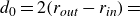 $d_0=2(r_{\textit{out}}-r_{\textit{in}})=$
24 mm of the annular duct and all frequencies and times are scaled by the characteristic convective frequency
$d_0=2(r_{\textit{out}}-r_{\textit{in}})=$
24 mm of the annular duct and all frequencies and times are scaled by the characteristic convective frequency
 $f_0={U_{\textit{in}}}/{d_0}$
, with
$f_0={U_{\textit{in}}}/{d_0}$
, with
 $U_{\textit{in}}$
= 15 m/s. Scaled quantities bear the superscript *. The stability map from the global analysis (2.14) is shown in figure 5: the scaled imaginary (i.e. eigenfrequency) and real parts (i.e. growth rate) of the eigenvalues
$U_{\textit{in}}$
= 15 m/s. Scaled quantities bear the superscript *. The stability map from the global analysis (2.14) is shown in figure 5: the scaled imaginary (i.e. eigenfrequency) and real parts (i.e. growth rate) of the eigenvalues
 $\lambda _o$
are plotted along the abscissa and ordinate, respectively. The flow is globally stable, meaning no self-sustained fluctuation develops around the mean flow.
$\lambda _o$
are plotted along the abscissa and ordinate, respectively. The flow is globally stable, meaning no self-sustained fluctuation develops around the mean flow.
Stability map (growth rate against eigenfrequency) for the Linearized Navier-Stokes Equations (LNSE) (2.14) (circles) and the network model (filled stars) of figure 6. The legend specifies the parameter variation, which is described in table 1. The arrows denote the shift of the two isolated eigenvalues (
 $\lambda _A$
and
$\lambda _A$
and
 $\lambda _B$
) when a parameter is varied.
$\lambda _B$
) when a parameter is varied.

Scaled dimensions of the configuration, inlet reflection coefficient (
 $\kappa _{\textit{in}}$
), swirl ratio (
$\kappa _{\textit{in}}$
), swirl ratio (
 ${Sw}$
) and Reynolds number (Re), for the base case (bold) and the parameter variation.
${Sw}$
) and Reynolds number (Re), for the base case (bold) and the parameter variation.

Sketch of the 1-D network model and the eigenmodes (pressure and velocity) and eigenvalues (A and B, stars in figure 5) computed from that network model (Emmert et al. Reference Emmert, Meindl, Jaensch and Polifke2016). Here, abs. refer to the absolute value.

The spectrum comprises a branch of decaying growth rate for increasing eigenfrequency, with two isolated eigenvalues –
 $\lambda _A$
and
$\lambda _A$
and
 $\lambda _B$
– dominating the spectrum at medium frequencies.
$\lambda _B$
– dominating the spectrum at medium frequencies.
The branch is not affected by the changes in lengths, reflection coefficient, swirler position and swirler intensity. Unlike the branch, the two isolated eigenvalues are affected by changes in dimension: a shortening of the mixing tube (case
 $L_{\textit{tube}}$
= 5.2) shifts
$L_{\textit{tube}}$
= 5.2) shifts
 $\lambda _A$
and
$\lambda _A$
and
 $\lambda _B$
to higher frequency, and an extension of the combustion chamber (case
$\lambda _B$
to higher frequency, and an extension of the combustion chamber (case
 $L_{\textit{chamber}}$
= 16.7) shifts them to lower frequency. Finally, turning the inlet to non-reflecting (case
$L_{\textit{chamber}}$
= 16.7) shifts them to lower frequency. Finally, turning the inlet to non-reflecting (case
 $r_{\textit{inlet}}$
= 0) dampens them. On the other hand, changes in the swirl intensity or swirler position, i.e. hydrodynamic parameters, do not affect them at all. Hence, these two eigenvalues are, at least partially, driven by acoustic waves sustained in the ensemble of the annular duct section and combustion chamber.
$r_{\textit{inlet}}$
= 0) dampens them. On the other hand, changes in the swirl intensity or swirler position, i.e. hydrodynamic parameters, do not affect them at all. Hence, these two eigenvalues are, at least partially, driven by acoustic waves sustained in the ensemble of the annular duct section and combustion chamber.
The eigenvalues predicted by the LNSE (2.14) are compared against a one-dimensional (1-D) acoustic network model based on interconnected state-space elements (Emmert et al. Reference Emmert, Meindl, Jaensch and Polifke2016) (filled stars in figure 5). This acoustic network simply models acoustic wave propagation without accounting for base flow effects and is, therefore, a cruder approximation compared with LNSE. However,
 $\lambda _A$
and
$\lambda _A$
and
 $\lambda _B$
from LNSE and the 1-D acoustic network are in good quantitative agreement. This confirms that both the eigenfrequency and the growth rate of
$\lambda _B$
from LNSE and the 1-D acoustic network are in good quantitative agreement. This confirms that both the eigenfrequency and the growth rate of
 $\lambda _A$
and
$\lambda _A$
and
 $\lambda _B$
are determined by acoustic parameters only: the lengths and boundary impedances for the frequency and the acoustic losses at boundaries for the growth rate.
$\lambda _B$
are determined by acoustic parameters only: the lengths and boundary impedances for the frequency and the acoustic losses at boundaries for the growth rate.
The acoustic eigenmodes obtained from the 1-D network model (figure 6) show that there is no complete decoupling of the annular duct section and the combustion chamber. This is expected since the area jump ratio,
 $r^*_{\textit{comb}}/(r^*_{\textit{out}} - r^*_{\textit{in}})=6.0$
, is moderate. Therefore, we cannot independently characterise the acoustic modes sustained in the annular duct section and combustion chamber. Nevertheless, the acoustic mode sustained in the annular duct section resembles a quarter-wave mode, with a quasi-pressure node at the area jump (figure 6). This is also reflected in the proximity of the imaginary part Im(
$r^*_{\textit{comb}}/(r^*_{\textit{out}} - r^*_{\textit{in}})=6.0$
, is moderate. Therefore, we cannot independently characterise the acoustic modes sustained in the annular duct section and combustion chamber. Nevertheless, the acoustic mode sustained in the annular duct section resembles a quarter-wave mode, with a quasi-pressure node at the area jump (figure 6). This is also reflected in the proximity of the imaginary part Im(
 $\lambda _A$
) = 0.73 with the frequency of a quarter-wave mode in the annular duct section:
$\lambda _A$
) = 0.73 with the frequency of a quarter-wave mode in the annular duct section:
 $f_{{1/4}}^*=0.76$
. We note that the negative growth rate is a consequence of acoustic losses at the boundaries.
$f_{{1/4}}^*=0.76$
. We note that the negative growth rate is a consequence of acoustic losses at the boundaries.
Changes in the length of the annular duct section and combustion chamber also change the respective growth rates of
 $\lambda _A$
and
$\lambda _A$
and
 $\lambda _B$
:
$\lambda _B$
:
 $\lambda _A$
is dominant for the base case, although
$\lambda _A$
is dominant for the base case, although
 $\lambda _B$
is dominant for the shorter annular duct section and longer combustion chamber. The analysis of the eigenmodes associated with
$\lambda _B$
is dominant for the shorter annular duct section and longer combustion chamber. The analysis of the eigenmodes associated with
 $\widetilde {\boldsymbol{q}}_{\!A}$
and
$\widetilde {\boldsymbol{q}}_{\!A}$
and
 $\widetilde {\boldsymbol{q}}_{\!B}$
carried out in Varillon et al. (Reference Varillon, Kaiser, Brokof, Oberleithner and Polifke2024) reveals that the least stable of these two eigenvalues is the one displaying shear-layer vortices at the tip of the annular duct exit. The subdominant mode, i.e. the second least stable, displays convective structures on
$\widetilde {\boldsymbol{q}}_{\!B}$
carried out in Varillon et al. (Reference Varillon, Kaiser, Brokof, Oberleithner and Polifke2024) reveals that the least stable of these two eigenvalues is the one displaying shear-layer vortices at the tip of the annular duct exit. The subdominant mode, i.e. the second least stable, displays convective structures on
 $\widetilde {\boldsymbol{u}}_x$
and
$\widetilde {\boldsymbol{u}}_x$
and
 $\widetilde {\omega }$
generation within the annular duct section rather than amplification in the shear layer in the combustion chamber (figure 7
a and b, lower halves).
$\widetilde {\omega }$
generation within the annular duct section rather than amplification in the shear layer in the combustion chamber (figure 7
a and b, lower halves).
Components of the eigenvector
 $\textrm {Re}(\widetilde {\boldsymbol{q}})$
:
$\textrm {Re}(\widetilde {\boldsymbol{q}})$
:
 $\widetilde {\boldsymbol{u}}_x$
(a),
$\widetilde {\boldsymbol{u}}_x$
(a),
 $\widetilde {\omega }$
(b),
$\widetilde {\omega }$
(b),
 $\widetilde {\boldsymbol{u}}_\theta$
(c) and
$\widetilde {\boldsymbol{u}}_\theta$
(c) and
 $\widetilde {p}$
(d), for
$\widetilde {p}$
(d), for
 $\widetilde {\boldsymbol{q}}_{\!A}$
(upper halves) and
$\widetilde {\boldsymbol{q}}_{\!A}$
(upper halves) and
 $\widetilde {\boldsymbol{q}}_{\!B}$
(lower halves) for the base configuration (cf. table 1). All fields are normalised to their respective maximum. Panels a to c are zoomed to the annular duct section and expansion. The swirler region where the axisymmetric swirler model is enforced ((2.3) and (2.4)) is circled in black. The iso-contours
$\widetilde {\boldsymbol{q}}_{\!B}$
(lower halves) for the base configuration (cf. table 1). All fields are normalised to their respective maximum. Panels a to c are zoomed to the annular duct section and expansion. The swirler region where the axisymmetric swirler model is enforced ((2.3) and (2.4)) is circled in black. The iso-contours
 $\widehat {\boldsymbol{u}}_x=0$
in white locate the recirculation regions.
$\widehat {\boldsymbol{u}}_x=0$
in white locate the recirculation regions.

Components of the eigenvector
 $\textrm {Re}(\widetilde {\boldsymbol{q}}_{\!A})$
:
$\textrm {Re}(\widetilde {\boldsymbol{q}}_{\!A})$
:
 $\widetilde {\boldsymbol{u}}_x$
(a),
$\widetilde {\boldsymbol{u}}_x$
(a),
 $\widetilde {\omega }$
(b),
$\widetilde {\omega }$
(b),
 $\widetilde {\boldsymbol{u}}_\theta$
(c) and
$\widetilde {\boldsymbol{u}}_\theta$
(c) and
 $\widetilde {p}$
(d), for Sw = 0.7 (upper halves) and Sw = 1.2 (lower halves), table 1. All fields are normalised to their respective maximum. Figures a to c are zoomed to the annular duct section and expansion. Black and with contours similar to figure 7.
$\widetilde {p}$
(d), for Sw = 0.7 (upper halves) and Sw = 1.2 (lower halves), table 1. All fields are normalised to their respective maximum. Figures a to c are zoomed to the annular duct section and expansion. Black and with contours similar to figure 7.

3.1. Swirl-induced non-normality
Although
 $\lambda _A$
is barely affected by an increase in swirl intensity (Sw = 0.75–1.2), the associated eigenvector
$\lambda _A$
is barely affected by an increase in swirl intensity (Sw = 0.75–1.2), the associated eigenvector
 $\widetilde {\boldsymbol{q}}_{\!A}$
changes. At low swirl intensity (Sw = 0.75),
$\widetilde {\boldsymbol{q}}_{\!A}$
changes. At low swirl intensity (Sw = 0.75),
 $\widetilde {\boldsymbol{u}}_{x_A}$
sees the superposition of two flow patterns, one typical of an axial acoustic mode and the other one typical of vorticity in the shear developing from the tip of the central rod, each of them being of similar magnitude (figure 8
a, upper halves). At higher swirl intensity (Sw = 1.2), the spatial structure of
$\widetilde {\boldsymbol{u}}_{x_A}$
sees the superposition of two flow patterns, one typical of an axial acoustic mode and the other one typical of vorticity in the shear developing from the tip of the central rod, each of them being of similar magnitude (figure 8
a, upper halves). At higher swirl intensity (Sw = 1.2), the spatial structure of
 $\widetilde {\boldsymbol{q}}_{\!A}$
is dominated by convective vortical patterns that overshadow the axial acoustic pattern on
$\widetilde {\boldsymbol{q}}_{\!A}$
is dominated by convective vortical patterns that overshadow the axial acoustic pattern on
 $\widetilde {\boldsymbol{u}}_x$
(figure 8
a lower halves). Similarly, axial vorticity is clearly visible on the pressure field in the high-swirl case (figure 8
d, lower half), although it is almost invisible in the low-swirl case (figure 8
d, upper half). Although the swirl number does not affect the global stability of the flow, it enhances a local convective-type instability developing in the shear layer trailing from the central rod.
$\widetilde {\boldsymbol{u}}_x$
(figure 8
a lower halves). Similarly, axial vorticity is clearly visible on the pressure field in the high-swirl case (figure 8
d, lower half), although it is almost invisible in the low-swirl case (figure 8
d, upper half). Although the swirl number does not affect the global stability of the flow, it enhances a local convective-type instability developing in the shear layer trailing from the central rod.
In the high-swirl case, these convective structures emanate from the point where the jet separates form the bluff body. Due to higher radial pressure gradient at higher swirl intensity, this separation point moves from the sharp tip of the bluff body (Sw = 0.7) to a position upstream in the duct (Sw = 1.2, figure 3). This change in the mean flow has a strong impact on the eigenvector structure, although it does not affect the associated eigenvalue. The interpretation is that the acoustics still sets the frequency, but the spatial structure of the response is dominated by hydrodynamic phenomena.
A modification of the condition number of the matrix evidences this change in the eigenvector without a drift of the eigenvalue. The condition number quantifies the non-orthogonality of the eigenvectors of a matrix: a normal matrix has orthogonal eigenvectors, and the less orthogonal the eigenvectors, the more non-normal the matrix (Trefethen & Embree Reference Trefethen and Embree2005). Orthogonal eigenvectors cannot interplay, and therefore the response norm of the associated dynamical system is bounded by the growth rate of the least stable eigenvalue at all times. On the contrary, non-orthogonal eigenvectors interplay linearly and produce transient growth – in the time domain – and resonance – in the frequency domain – which are not predictable by the eigenvalues alone (Trefethen et al. Reference Trefethen, Trefethen, Reddy and Driscoll1993). The condition number of a matrix can be further split into individual condition numbers associated with each eigenvalue
 \begin{equation} \kappa (\lambda _o)=\dfrac {1}{|\langle \widetilde {\boldsymbol{q}}_o^\dagger , \widetilde {\boldsymbol{q}}_o \rangle |},\quad \|\widetilde {\boldsymbol{q}}_o\|=\|\widetilde {\boldsymbol{q}}_o^\dagger \|=1, \end{equation}
which are the contributions of each eigenvalue to the matrix condition number. The vector
 $\widetilde {\boldsymbol{q}}_o^\dagger$
is the left eigenvector associated with the eigenvalue
$\widetilde {\boldsymbol{q}}_o^\dagger$
is the left eigenvector associated with the eigenvalue
 $\lambda _o$
(2.14), also called the adjoint eigenvector. The scalar product in (3.1) is the one defining the
$\lambda _o$
(2.14), also called the adjoint eigenvector. The scalar product in (3.1) is the one defining the
 $L_2$
norm
$L_2$
norm
 \begin{align} \langle \boldsymbol{f}, \boldsymbol{g} \rangle = \int _V \boldsymbol{f}^H \boldsymbol{g} \text{d}V, \end{align}
for
 $\boldsymbol{f}$
and
$\boldsymbol{f}$
and
 $\boldsymbol{g}$
two vectors, with
$\boldsymbol{g}$
two vectors, with
 $V$
the domain and
$V$
the domain and
 $H$
denoting the conjugate transpose. Equation (3.1) illustrates that the eigenvalue condition number is minimal when the right and left eigenvectors are identical. This is a property of normal matrices. Consistently, the more the left and right eigenvectors depart from one another, the higher
$H$
denoting the conjugate transpose. Equation (3.1) illustrates that the eigenvalue condition number is minimal when the right and left eigenvectors are identical. This is a property of normal matrices. Consistently, the more the left and right eigenvectors depart from one another, the higher
 $\kappa (\lambda _o)$
.
$\kappa (\lambda _o)$
.
The eigenvalue condition number
 $\kappa$
is computed for
$\kappa$
is computed for
 $\lambda _A$
and
$\lambda _A$
and
 $\lambda _B$
in the low- and high-swirl cases in table 2 and shows an increase of one order of magnitude. This increase in non-normality with swirl intensity confirms that the dynamical behaviour of the linear system driving the evolution of small fluctuations (2.12) is changing beyond eigenvalues.
$\lambda _B$
in the low- and high-swirl cases in table 2 and shows an increase of one order of magnitude. This increase in non-normality with swirl intensity confirms that the dynamical behaviour of the linear system driving the evolution of small fluctuations (2.12) is changing beyond eigenvalues.
Measure of non-normality
 $\kappa$
for
$\kappa$
for
 $\lambda _A$
and
$\lambda _A$
and
 $\lambda _B$
.
$\lambda _B$
.

This increase in
 $\kappa$
is illustrated in figure 9, which displays the local
$\kappa$
is illustrated in figure 9, which displays the local
 $L_2$
norm
$L_2$
norm
 \begin{equation} \mathfrak{d}_{L_2} = \langle \widetilde {\boldsymbol{f}}, \widetilde {\boldsymbol{f}} \rangle \end{equation}
for
 $\widetilde {\boldsymbol{f}}=\widetilde {\boldsymbol{q}}_{\!A}$
and
$\widetilde {\boldsymbol{f}}=\widetilde {\boldsymbol{q}}_{\!A}$
and
 $\widetilde {\boldsymbol{q}}_{\!A}^\dagger$
. The higher the swirl number, the larger the dissociation between the spatial support of the left and right eigenvectors: at higher swirl intensity,
$\widetilde {\boldsymbol{q}}_{\!A}^\dagger$
. The higher the swirl number, the larger the dissociation between the spatial support of the left and right eigenvectors: at higher swirl intensity,
 $\widetilde {\boldsymbol{q}}_{\!A}$
has more activity downstream in the wake of the bluff body, while the activity of
$\widetilde {\boldsymbol{q}}_{\!A}$
has more activity downstream in the wake of the bluff body, while the activity of
 $\widetilde {\boldsymbol{q}}^\dagger _A$
is shifted upstream in the swirler region. This dissociation between the left and right eigenvector is qualified as convection-type non-normality by Chomaz (Reference Chomaz2005) and Brandt et al. (Reference Brandt, Sipp, Pralits and Marquet2011).
$\widetilde {\boldsymbol{q}}^\dagger _A$
is shifted upstream in the swirler region. This dissociation between the left and right eigenvector is qualified as convection-type non-normality by Chomaz (Reference Chomaz2005) and Brandt et al. (Reference Brandt, Sipp, Pralits and Marquet2011).
The non-normality of the eigenvector basis brought by that eigenvalue may trigger non-modal amplification, as will be investigated in § 4. The consequences of an increased non-normality are (i) a stronger transient amplification of asymptotically stable initial perturbations and (ii) a higher sensitivity of the spectrum to modification of the mean flow: the minimum size of the mean flow perturbation to shift an eigenvalue to the unstable half-plane is smaller for higher non-normality of the flow (Trefethen et al. Reference Trefethen, Trefethen, Reddy and Driscoll1993). Finally, (iii) the higher non-normality may enhance the amplification of external forcing through resonance. This last consequence is investigated in the next section via the resolvent analysis.
Local
 $L_2$
norm ((3.3)) of the right eigenvectors (upper halves) and left eigenvectors (lower halves). Panels show the Sw = 0.75 case (a) and Sw = 1.2 case (b). The visualisation window is centred on the region on activity of the right and left eigenvectors.
$L_2$
norm ((3.3)) of the right eigenvectors (upper halves) and left eigenvectors (lower halves). Panels show the Sw = 0.75 case (a) and Sw = 1.2 case (b). The visualisation window is centred on the region on activity of the right and left eigenvectors.

4. Gain of the resolvent
In this section, equation (2.16) is forced with a source term
 $\widehat {\kern-2pt \boldsymbol{f}}$
chosen as an axial or azimuthal body force. The forcing is restricted to either the combustion chamber or the annular duct section. The extensor matrix in equations (3.1) and (2.18) maps the forcing subspace to the full state space of (2.13) according to the abovementioned cases. The optimal gains (2.17) at various frequencies are gathered in a gain curve. The chosen norm of the forcing is the
$\widehat {\kern-2pt \boldsymbol{f}}$
chosen as an axial or azimuthal body force. The forcing is restricted to either the combustion chamber or the annular duct section. The extensor matrix in equations (3.1) and (2.18) maps the forcing subspace to the full state space of (2.13) according to the abovementioned cases. The optimal gains (2.17) at various frequencies are gathered in a gain curve. The chosen norm of the forcing is the
 $L_2$
norm
$L_2$
norm
 \begin{equation} \|\widehat {f}\|_f=\int _V \widehat {f}^{\,2} \text{d}V. \end{equation}
The strength of the response
 $\|\widehat {q}\|_q$
is successively measured with two different norms to establish the independency of the gain curve on the response norm. The first choice is the standard
$\|\widehat {q}\|_q$
is successively measured with two different norms to establish the independency of the gain curve on the response norm. The first choice is the standard
 $L_2$
norm
$L_2$
norm
 \begin{equation} \|\widehat {\boldsymbol{q}} \|_{L_2} = \int _V \widehat {\boldsymbol{q}}^H \widehat {\boldsymbol{q}} \text{d}V, \end{equation}
and the second choice is Chu’s energy (Chu Reference Chu1965)
 \begin{equation} \|\widehat {\boldsymbol{q}} \|_{\textit{Chu}} = \int _V \left (\overline {\rho } \widehat {\boldsymbol{u}}^2 + \dfrac {\overline {c}^2\widehat {p}^2}{\gamma \overline {\rho }} + \dfrac {\overline {\rho }\overline {C}_v \widehat {T}^2}{\overline {T}} \right )\text{d}V, \end{equation}
with
 $\gamma$
the ratio of specific heat. In what follows, the forcing is successively applied in the combustion chamber and in the annular duct section.
$\gamma$
the ratio of specific heat. In what follows, the forcing is successively applied in the combustion chamber and in the annular duct section.
4.1. Forcing on the axial momentum equation in the combustion chamber
In this subsection, the forcing term
 $\widehat {\kern-2pt\boldsymbol{f}}$
is applied in the combustion chamber only, on the axial momentum conservation equation. The magnitude of the gains (2.17) for two different norms cannot be compared, however, the relative variations over frequencies are comparable. When scaled to their maximum, gain curves from the
$\widehat {\kern-2pt\boldsymbol{f}}$
is applied in the combustion chamber only, on the axial momentum conservation equation. The magnitude of the gains (2.17) for two different norms cannot be compared, however, the relative variations over frequencies are comparable. When scaled to their maximum, gain curves from the
 $L_2$
norm and Chu’s energy yield the same gain variations throughout the frequency range (‘Chu’ and ‘
$L_2$
norm and Chu’s energy yield the same gain variations throughout the frequency range (‘Chu’ and ‘
 $L_2$
’ in figure 10
a). Hence, analysis of the gain curves is considered independent of the choice of the norm. In the following, we retain Chu’s energy as the response norm as it naturally splits into the ‘compression’ and the ‘kinetic’ part, as defined in Chu (Reference Chu1965). This will benefit the rest of the analysis, particularly identifying the hydrodynamic and acoustic responses.
$L_2$
’ in figure 10
a). Hence, analysis of the gain curves is considered independent of the choice of the norm. In the following, we retain Chu’s energy as the response norm as it naturally splits into the ‘compression’ and the ‘kinetic’ part, as defined in Chu (Reference Chu1965). This will benefit the rest of the analysis, particularly identifying the hydrodynamic and acoustic responses.
Optimal gain of the resolvent (2.17): (a) for the ‘base case’ (parameters are described in the first row of table 1) with
 $L_2$
norm, Chu’s norm and two semi-norms: the ‘compression’ and ‘kinetic’ parts of Chu’s energy, as defined in Chu (Reference Chu1965). Each curve is rescaled to its maximum over the frequency range considered; (b) for the various cases defined in table 1 with Chu’s norm. The legend specifies the parameter variation.
$L_2$
norm, Chu’s norm and two semi-norms: the ‘compression’ and ‘kinetic’ parts of Chu’s energy, as defined in Chu (Reference Chu1965). Each curve is rescaled to its maximum over the frequency range considered; (b) for the various cases defined in table 1 with Chu’s norm. The legend specifies the parameter variation.

The gain curves show two resonances, in which peak frequencies depend on the length of the annular duct and the chamber (figure 10
b). In addition, the resonance peaks occur at the eigenfrequencies of
 $\lambda _A$
and
$\lambda _A$
and
 $\lambda _B$
, as analysed in Varillon et al. (Reference Varillon, Kaiser, Brokof, Oberleithner and Polifke2024). These resonances do not occur when the inlet is also non-reflecting (the outlet is non-reflecting in all cases). This is due to acoustic losses at both inlet and outlet.
$\lambda _B$
, as analysed in Varillon et al. (Reference Varillon, Kaiser, Brokof, Oberleithner and Polifke2024). These resonances do not occur when the inlet is also non-reflecting (the outlet is non-reflecting in all cases). This is due to acoustic losses at both inlet and outlet.
The changes in the hydrodynamics, i.e. the swirl intensity and swirler position, do not affect the gain curve for the forcing in the combustion chamber. In addition, when
 $\|\widehat {\boldsymbol{q}}\|_{\textit{Chu}}$
is restricted to the ‘kinetic’ part of Chu’s energy, as defined in Chu (Reference Chu1965), the gain curve does not show any resonance, except at low frequency (figure 10
a). In contrast, the restriction of
$\|\widehat {\boldsymbol{q}}\|_{\textit{Chu}}$
is restricted to the ‘kinetic’ part of Chu’s energy, as defined in Chu (Reference Chu1965), the gain curve does not show any resonance, except at low frequency (figure 10
a). In contrast, the restriction of
 $\|\widehat {\boldsymbol{q}}\|_{\textit{Chu}}$
to the ‘compression’ part of Chu’s energy collapses with the gain curves from
$\|\widehat {\boldsymbol{q}}\|_{\textit{Chu}}$
to the ‘compression’ part of Chu’s energy collapses with the gain curves from
 $\|\widehat {\boldsymbol{q}}\|_{\textit{Chu}}$
and
$\|\widehat {\boldsymbol{q}}\|_{\textit{Chu}}$
and
 $\|\widehat {\boldsymbol{q}}\|_{L_2}$
. These observations support the dominance of compressibility effects, i.e. acoustics, in the frequency selection mechanism.
$\|\widehat {\boldsymbol{q}}\|_{L_2}$
. These observations support the dominance of compressibility effects, i.e. acoustics, in the frequency selection mechanism.
Section 3.1 evidenced an increased non-normality of the basis of eigenvectors induced by increased swirl intensity. This increased non-normality does not affect the dominant amplification mechanism triggered by an axial body force in the combustion chamber. Firstly, the gain curves at low and increased swirl intensity are similar. Secondly, the optimal forcing and response fields are also similar for both swirl intensities (figure 11). In particular, the regions of high activity of the forcing and response are not further apart for the increased swirl. An increased spatial separation of forcing and response would have indicated a non-modal amplification. Therefore, the dominant amplification process for a body force in the combustion chamber is of modal kind, i.e. driven by an eigenvalue. Although the amplification process implies shear-layer vortices (figure 11 b), it is triggered by an acoustic mode, hence its modal nature.
(a) Optimal forcing: axial body force in the combustion chamber, (b) optimal response: real part of
 $\widehat {\boldsymbol{u}}_x$
. Upper halves: Sw = 0.7, lower halves: Sw = 1.2.
$\widehat {\boldsymbol{u}}_x$
. Upper halves: Sw = 0.7, lower halves: Sw = 1.2.

4.2. Forcing in the mixing tube
In this subsection the forcing term
 $\widehat {f}$
is applied in the mixing tube only, in the axial or the azimuthal momentum conservation equation. Three cases are described in figure 12: forcing on the axial momentum at low (‘xl’) and high (‘xh’) swirls, same but with a non-reflecting inlet (‘xnl’ and ‘xnh’) and forcing on the azimuthal momentum (‘
$\widehat {f}$
is applied in the mixing tube only, in the axial or the azimuthal momentum conservation equation. Three cases are described in figure 12: forcing on the axial momentum at low (‘xl’) and high (‘xh’) swirls, same but with a non-reflecting inlet (‘xnl’ and ‘xnh’) and forcing on the azimuthal momentum (‘
 $\theta$
l’ and ‘
$\theta$
l’ and ‘
 $\theta$
h’).
$\theta$
h’).
In contrast to forcing in the combustion chamber, a forcing in the mixing tube reveals some over-amplification in the high-swirl case compared with the low-swirl case. Compared with the case ‘xl’, the case ‘xh’ displays a gain separation: the optimal gain dominates the suboptimal gain curves with a plateau over a wide range of frequencies (figure 12
a, yellow gain curve). This plateau is superimposed with a resonance peak at the frequency of the dominating eigenvalue
 $\lambda _A$
. Such a wide plateau is typical of non-modal amplification. The non-reflecting cases ‘xnh’ and ‘xnl’ display the same behaviour except the resonance (figure 12
b), which is understandable since no acoustic mode is sustained without reflection at the inlet and outlet.
$\lambda _A$
. Such a wide plateau is typical of non-modal amplification. The non-reflecting cases ‘xnh’ and ‘xnl’ display the same behaviour except the resonance (figure 12
b), which is understandable since no acoustic mode is sustained without reflection at the inlet and outlet.
In these two cases (figure 12 a,b), a drastic change of the optimal forcing, and to a lesser extent the optimal response, occurs for the increased swirl. While the optimal forcing and responses partially overlap at the low swirl intensity, their spatial support is mostly dissociated in the high-swirl case: the optimal forcing is active upstream and at the flow separation point, and the optimal response is active only downstream of the flow separation point. Such a spatial separation between optimal forcing and responses characterises convective type non-normality (Marquet et al. Reference Marquet, Lombardi, Chomas, Sipp and Jacquin2009).
These two cases – forcing on the axial momentum equation with a hard or non-reflecting inlet – present an increased gain separation, i.e. the optimal gain is well separated from the suboptimal gains for a higher swirl. Concurrently, the optimal responses become dominated by shear-layer vortices shed from the separation point and amplified over a few wavelengths. This is visible in figure 12(a) on the pressure field, and in figure 12(b) on the axial velocity field.
This result is complemented by the high amplification and gain separation in the case of a forcing on the azimuthal momentum (case ‘
 $\theta$
h’ figure 12
c). The increased swirl intensity generates a resonance corresponding to the longitudinal acoustic mode. The absence of resonance in the ‘
$\theta$
h’ figure 12
c). The increased swirl intensity generates a resonance corresponding to the longitudinal acoustic mode. The absence of resonance in the ‘
 $\theta$
l’ case is understandable since the azimuthal component of momentum conservation does not produce axial acoustics. The occurrence of that axial acoustic resonance suggests that a coupling of azimuthal to axial momentum fluctuations is at stake and active only at high swirl intensity due to the high sensitivity of the flow separation point.
$\theta$
l’ case is understandable since the azimuthal component of momentum conservation does not produce axial acoustics. The occurrence of that axial acoustic resonance suggests that a coupling of azimuthal to axial momentum fluctuations is at stake and active only at high swirl intensity due to the high sensitivity of the flow separation point.
In the high-swirl cases (‘xh’, ‘xnh’ and ‘
 $\theta$
h’ in figure 12), the responses emanate from the flow separation point, rather than from the swirler at lower swirl intensity. The flow separation point also clusters the forcing in these two cases, indicating that the most efficient way to amplify perturbations in the high-swirl case is to perturb the flow separation point in the axial direction.
$\theta$
h’ in figure 12), the responses emanate from the flow separation point, rather than from the swirler at lower swirl intensity. The flow separation point also clusters the forcing in these two cases, indicating that the most efficient way to amplify perturbations in the high-swirl case is to perturb the flow separation point in the axial direction.
Gain curves with the optimal gain and suboptimal gains (shaded). Forcing on the mixing tube for low (black) and high (yellow) swirl intensity. Forcing (a) on the axial momentum with closed inlet, (b) on the axial momentum with non-reflecting inlet and (c) on the azimuthal momentum with closed inlet.

4.2.1. Sensitivity of the resolvent gain
The qualitative observation on the sensitivity of the flow separation point is now investigated in a systematic way via the sensitivity of the resolvent gain. For globally unstable modes, the core of the instability, usually referred to as the wavemaker region, is identified by the structural sensitivity that identifies regions of strong internal localised feedback of the flow on itself (Giannetti & Luchini Reference Giannetti and Luchini2007; Schmid & Brandt Reference Schmid and Brandt2014). For globally stable modes, the concept of wavemaker region has been extended by Fosas de Pando et al. (Reference de Pando, Miguel and Lele2014) and Qadri & Schmid (Reference Qadri and Schmid2017) to the sensitivity of the resolvent gain. The optimal forcing
 $\widehat {\kern-2pt\boldsymbol{f}}$
and corresponding response
$\widehat {\kern-2pt\boldsymbol{f}}$
and corresponding response
 $\widehat {\boldsymbol{q}}$
obtained from the eigenvalue problem (2.18) are equivalently the left and right singular vectors associated with the singular value
$\widehat {\boldsymbol{q}}$
obtained from the eigenvalue problem (2.18) are equivalently the left and right singular vectors associated with the singular value
 $ G(\omega )$
of the resolvent operator
$ G(\omega )$
of the resolvent operator
 ${H}={F}_{\!\boldsymbol{q}}\textit{RBF}_{\!\boldsymbol{f}}$
 \begin{equation} G(\omega ) = \widehat {\boldsymbol{q}}^H {H}\widehat {\kern-2pt\boldsymbol{f}}, \end{equation}
with
 ${F}_{\!\boldsymbol{q}}$
and
${F}_{\!\boldsymbol{q}}$
and
 ${F}_{\!\boldsymbol{f}}$
the Cholesky decompositions of
${F}_{\!\boldsymbol{f}}$
the Cholesky decompositions of
 ${Q}_{\boldsymbol{q}}$
and
${Q}_{\boldsymbol{q}}$
and
 ${Q}_{\!\boldsymbol{f}}$
, respectively:
${Q}_{\!\boldsymbol{f}}$
, respectively:
 ${Q}_{\boldsymbol{q}}={F}_{\!\boldsymbol{q}}^H{F}_{\!\boldsymbol{q}}$
and
${Q}_{\boldsymbol{q}}={F}_{\!\boldsymbol{q}}^H{F}_{\!\boldsymbol{q}}$
and
 ${Q}_{\!\boldsymbol{f}}={F}_{\!\boldsymbol{f}}^H{F}_{\!\boldsymbol{f}}$
. For the sake of clarity, the frequency dependence
${Q}_{\!\boldsymbol{f}}={F}_{\!\boldsymbol{f}}^H{F}_{\!\boldsymbol{f}}$
. For the sake of clarity, the frequency dependence
 $\omega$
is dropped in the remainder of this section (
$\omega$
is dropped in the remainder of this section (
 $G(\omega )=G$
).
$G(\omega )=G$
).
A change in the mean flow generating a fluctuation
 $\delta {H}$
of the resolvent operator induces a modification of the gain (see Appendix C)
$\delta {H}$
of the resolvent operator induces a modification of the gain (see Appendix C)
 \begin{equation} \delta G = \textit{Re} \big (\widehat {\boldsymbol{q}}^H \delta {H}\widehat {\kern-2pt\boldsymbol{f}}\,\big ),\quad \text{or equivalently} \quad \dfrac {-\delta G}{G^2} = \textit{Re} \big(\,\widehat {\kern-2pt\boldsymbol{f}}^H{B}^H{F}_{\!\boldsymbol{f}}^H\delta ({R}^{-1}){F}_{\!\boldsymbol{q}}\widehat {\boldsymbol{q}}\big). \end{equation}
Following the idea developed by Giannetti & Luchini (Reference Giannetti and Luchini2007) and Schmid & Brandt (Reference Schmid and Brandt2014) for the structural sensitivity, and extended by Fosas de Pando et al. (Reference de Pando, Miguel and Lele2014) and Qadri & Schmid (Reference Qadri and Schmid2017) for the resolvent sensitivity, we are interested in a perturbation
 $\delta \mathsf{L}$
adding a local feedback of the flow velocity to the momentum conservation equation. Since the chosen frequency and the mass matrix are unaffected by changes in the mean flow, we assume
$\delta \mathsf{L}$
adding a local feedback of the flow velocity to the momentum conservation equation. Since the chosen frequency and the mass matrix are unaffected by changes in the mean flow, we assume
 $\delta ({R}^{-1} )=-\delta {L}$
, where the matrix
$\delta ({R}^{-1} )=-\delta {L}$
, where the matrix
 $\delta {L}$
corresponds to the discretisation of the perturbation
$\delta {L}$
corresponds to the discretisation of the perturbation
 $\delta \mathsf{L}$
of the space continuous linearised Navier–Stokes equations
$\delta \mathsf{L}$
of the space continuous linearised Navier–Stokes equations
 $\mathsf{L}$
, (2.12). The perturbation
$\mathsf{L}$
, (2.12). The perturbation
 $\delta \mathsf{L}$
is localised at
$\delta \mathsf{L}$
is localised at
 $\boldsymbol{x}_0$
and reads
$\boldsymbol{x}_0$
and reads
 \begin{equation} \widehat {\kern-2pt\boldsymbol{f}}^H{B}^H{F}_{\!\boldsymbol{f}}^H\delta \mathsf{L}{F}_{\!\boldsymbol{q}}\widehat {\boldsymbol{q}} = \widehat {\kern-2pt\boldsymbol{f}}_x^H \delta (\boldsymbol{ x}-\boldsymbol{x}_0){F}_{\!\boldsymbol{q}}^{\boldsymbol{u}_x}\widehat {\boldsymbol{u}}_x + \widehat {\kern-2pt\boldsymbol{f}}_\theta ^H \delta (\boldsymbol{x}-\boldsymbol{ x}_0){F}_{\!\boldsymbol{q}}^{\boldsymbol{u}_\theta }\widehat {\boldsymbol{u}}_\theta , \end{equation}
with
 $\delta (\boldsymbol{x}-\boldsymbol{x}_0)$
the Dirac function around
$\delta (\boldsymbol{x}-\boldsymbol{x}_0)$
the Dirac function around
 $\bf x_0$
, and
$\bf x_0$
, and
 ${F}_{\!\boldsymbol{q}}^{\boldsymbol{u}_x}$
and
${F}_{\!\boldsymbol{q}}^{\boldsymbol{u}_x}$
and
 ${F}_{\!\boldsymbol{q}}^{\boldsymbol{u}_\theta }$
represent the reduction of the matrix
${F}_{\!\boldsymbol{q}}^{\boldsymbol{u}_\theta }$
represent the reduction of the matrix
 ${F}_{\!\boldsymbol{q}}$
to the axial and azimuthal velocity components, respectively. Therefore,
${F}_{\!\boldsymbol{q}}$
to the axial and azimuthal velocity components, respectively. Therefore,
 \begin{equation} \delta G = G^2 \textit{Re} \big (\, \widehat {\kern-2pt\boldsymbol{f}}_x^H(\boldsymbol{x}_0){F}_{\!\boldsymbol{q}}^{\boldsymbol{u}_x}\widehat {\boldsymbol{u}}_x(\boldsymbol{x}_0) + \widehat {\kern-2pt\boldsymbol{f}}_\theta ^H(\boldsymbol{x}_0) {F}_{\!\boldsymbol{q}}^{\boldsymbol{u}_\theta }\widehat {\boldsymbol{u}}_\theta (\boldsymbol{x}_0) \big). \end{equation}
By inspecting the right-hand side of (4.7) for
 $\boldsymbol{x}_0$
spanning the flow domain, we identify regions where the gain is highly sensitive to local feedback. In these regions, the optimal response
$\boldsymbol{x}_0$
spanning the flow domain, we identify regions where the gain is highly sensitive to local feedback. In these regions, the optimal response
 $\widehat {\boldsymbol{q}}$
aligns with the optimal forcing
$\widehat {\boldsymbol{q}}$
aligns with the optimal forcing
 $\widehat {\kern-2pt\boldsymbol{f}}$
, revealing a self-amplification mechanism, i.e. a wavemaker region.
$\widehat {\kern-2pt\boldsymbol{f}}$
, revealing a self-amplification mechanism, i.e. a wavemaker region.
Figure 13 shows the gain sensitivity
 $\delta G$
for
$\delta G$
for
 $\boldsymbol{x}_0$
at each location of the flow domain, in the case of a forcing in the annular duct section, to the axial momentum conservation. The gain sensitivity increases and clusters at the flow separation point at higher swirl numbers. This is a confirmation that, once the separation point moves upstream of the bluff body tip due to high swirl intensity, (i) the gain becomes highly sensitive to the mean flow changes near the separation point, and (ii) the shear layer at that location becomes the core of the spatial shear-layer vortices developing downstream. These shear-layer vortices grow over a few wavelengths before decaying. This flow structure shares similarities with the convective Kelvin–Helmholtz (KH) instability (Schmidt et al. Reference Schmidt, Towne, Rigas, Colonius and Brès2018). The occurrence of a spatial KH instability is supported by the presence of the backward-facing step that generates an inflection point in the axial velocity profile, which is a necessary condition (Rayleigh’s criterion (Schmid & Henningson Reference Schmid and Henningson2001)). This standard scenario, usually observed in jets expanding in an open environment, is here perturbed by the confinement of the outer walls of the combustion chamber against which the expanding jet collides due to the swirl motion. However, other mechanisms inducing shear-layer vortices are not ruled out.
$\boldsymbol{x}_0$
at each location of the flow domain, in the case of a forcing in the annular duct section, to the axial momentum conservation. The gain sensitivity increases and clusters at the flow separation point at higher swirl numbers. This is a confirmation that, once the separation point moves upstream of the bluff body tip due to high swirl intensity, (i) the gain becomes highly sensitive to the mean flow changes near the separation point, and (ii) the shear layer at that location becomes the core of the spatial shear-layer vortices developing downstream. These shear-layer vortices grow over a few wavelengths before decaying. This flow structure shares similarities with the convective Kelvin–Helmholtz (KH) instability (Schmidt et al. Reference Schmidt, Towne, Rigas, Colonius and Brès2018). The occurrence of a spatial KH instability is supported by the presence of the backward-facing step that generates an inflection point in the axial velocity profile, which is a necessary condition (Rayleigh’s criterion (Schmid & Henningson Reference Schmid and Henningson2001)). This standard scenario, usually observed in jets expanding in an open environment, is here perturbed by the confinement of the outer walls of the combustion chamber against which the expanding jet collides due to the swirl motion. However, other mechanisms inducing shear-layer vortices are not ruled out.

5. Discussion of the resolvent analysis results
5.1. Amplification mechanisms in the combustion chamber
The forcing in the combustion chamber evidenced an optimal amplification of a modal kind. This is consistent with the compressible – or acoustic – nature of the dominant amplification analysed in the global stability analysis (§ 3). Acoustic fluctuations propagate through a wave equation of symmetrical nature (up to the boundary conditions), yielding orthogonal acoustic eigenmodes in the linear regime. That is why acoustics is a phenomenon of modal nature. This also explains that, for a forcing in the combustion chamber, the amplification mechanisms are not affected by the swirl-enhanced non-normality at higher swirl intensity. The exact shape of these axial acoustic modes depends, however, on the impedances of the inlet and outlet (here with partial flow blockage).
The optimal forcing in the combustion chamber is the superposition of a longitudinal acoustic-like pattern, i.e. a diffuse and smooth field with changes in the longitudinal direction, and a forcing similar to the one obtained in the incompressible case (see, e.g. Schmidt et al. Reference Schmidt, Towne, Rigas, Colonius and Brès2018, figure 6a). The non-normality of the KH mode alone in the incompressible models is overshadowed compressibility effects. This optimal forcing also resembles the acoustic pressure field generated by a HHR fluctuation in the combustion chamber, as already noted by Varillon et al. (Reference Varillon, Kaiser, Brokof, Oberleithner and Polifke2024). Consequently, this optimal forcing is likely to be triggered by HHR fluctuations in a reacting configuration.
5.2. Non-modal amplification
Non-modal amplification has already been identified in swirling flows. For example, Antkowiak & Brancher (Reference Antkowiak and Brancher2004), Pradeep & Hussain (Reference Pradeep and Hussain2006) and Heaton & Peake (Reference Heaton and Peake2007) report on transient amplification of kinetic energy of small disturbances in subcritical vortices in the temporal domain. Therefore, the present results confirm existing results, although in another configuration. The present study also evidences non-modal amplification from the condition number of specific eigenvalues, which identifies the mechanism that drives the non-modal amplification, and the resolvent analysis, rather than from temporal amplification.
Forcing in the mixing tube evidenced shear-layer vortices as a main feature of the optimal amplification, that share similarities with KH instability. The KH instability was already identified as responsible for gain separation in a subsonic non-swirling jet for
 $0.2\leqslant St \leqslant 2$
, with a peak amplification at
$0.2\leqslant St \leqslant 2$
, with a peak amplification at
 $St=0.6$
, for the azimuthally symmetrical mode (Schmidt et al. Reference Schmidt, Towne, Rigas, Colonius and Brès2018; Kaiser, Lesshafft & Oberleithner Reference Kaiser, Lesshafft and Oberleithner2019; Pickering et al. Reference Pickering, Rigas, Nogueira, Cavalieri, Schmidt and Colonius2020). In addition, low-rank behaviour and the KH mechanism are absent at low frequencies in the previously cited references. These results are consistent with the present observations. Adding a swirl motion to the jet considered in the above-cited works does not change the nature of the shear in the axial direction, and the additional shear in the azimuthal direction does not generate transverse shear-layer vortices for the azimuthally symmetrical modes considered in the present work. Consequently, we credit the increased gain separation in the case ‘
$St=0.6$
, for the azimuthally symmetrical mode (Schmidt et al. Reference Schmidt, Towne, Rigas, Colonius and Brès2018; Kaiser, Lesshafft & Oberleithner Reference Kaiser, Lesshafft and Oberleithner2019; Pickering et al. Reference Pickering, Rigas, Nogueira, Cavalieri, Schmidt and Colonius2020). In addition, low-rank behaviour and the KH mechanism are absent at low frequencies in the previously cited references. These results are consistent with the present observations. Adding a swirl motion to the jet considered in the above-cited works does not change the nature of the shear in the axial direction, and the additional shear in the azimuthal direction does not generate transverse shear-layer vortices for the azimuthally symmetrical modes considered in the present work. Consequently, we credit the increased gain separation in the case ‘
 $\theta$
h’ (figure 12) as associated with enhanced spatially developing shear-layer vortices.
$\theta$
h’ (figure 12) as associated with enhanced spatially developing shear-layer vortices.
The spatial separation of optimal forcing and response denoting a convective-type non-normality discussed above is also the mark of a (local) spatial instability (Schmidt et al. Reference Schmidt, Towne, Rigas, Colonius and Brès2018). Although the global modes are stable, this convective instability can be associated with KH modes, typically amplified over a few vortex wavelengths downstream of the area expansion. In the present case, these vortices follow the streamlines that collide with the outer walls due to the flow expansion driven by the rotational motion.
5.3. RANS modelling
A reason for shear-layer vortex enhancement at higher swirl intensity is the increased sensitivity at the flow separation point. This flow separation point is here predicted by a RANS
 $k-\omega$
SST model. This model relies on the Boussinesq approximation, which is not fully justified in swirling flows because of the increased anisotropy of the Reynolds stress tensor. Therefore, the prediction of the detachment point shifting upstream in the annular duct at higher swirl should be made carefully.
$k-\omega$
SST model. This model relies on the Boussinesq approximation, which is not fully justified in swirling flows because of the increased anisotropy of the Reynolds stress tensor. Therefore, the prediction of the detachment point shifting upstream in the annular duct at higher swirl should be made carefully.
The present model flow is representative of the BRS burner, which features such a flow separation upstream from the tip of the bluff body under some flow conditions (Tay-Wo-Chong & Polifke Reference Tay-Wo-Chong and Polifke2013). Therefore, the prediction of a separation point shifting inside the annular duct is deemed realistic despite the use of a
 $k-\omega$
SST model. A tentative explanation for this comes from the confinement over a short radius and the low shear in the annular duct. Under such conditions, radial momentum balance is dominated by the pressure gradient rather than Reynolds stress. This statement does not hold in the high shear wake behind the expansion, where the radial pressure gradient is lower, such that the Reynold stress is dominant.
$k-\omega$
SST model. A tentative explanation for this comes from the confinement over a short radius and the low shear in the annular duct. Under such conditions, radial momentum balance is dominated by the pressure gradient rather than Reynolds stress. This statement does not hold in the high shear wake behind the expansion, where the radial pressure gradient is lower, such that the Reynold stress is dominant.
Beyond the prediction of this binary transition (is the flow separating from the bluff body at its tip or upstream?), we cannot claim that the
 $k-\omega$
SST model predicts the accurate position of the detachment point in the annular duct. However, the qualitative picture described in the results does not depend on knowledge of the accurate distance of the detachment point from the tip of the central rod. Therefore, despite the fact that the RANS modelling of the mean-field
$k-\omega$
SST model predicts the accurate position of the detachment point in the annular duct. However, the qualitative picture described in the results does not depend on knowledge of the accurate distance of the detachment point from the tip of the central rod. Therefore, despite the fact that the RANS modelling of the mean-field
 $\overline {\boldsymbol{q}}$
cannot be assumed as quantitatively predictive, the flow topologies at low and high swirl numbers are deemed sufficiently realistic for the analysis.
$\overline {\boldsymbol{q}}$
cannot be assumed as quantitatively predictive, the flow topologies at low and high swirl numbers are deemed sufficiently realistic for the analysis.
In addition, the presented methodology gains in consistency by using a RANS mean field, since the evolution equations for the linear perturbations stem from the equations actually yielding the mean-field
 $\overline {\boldsymbol{q}}$
. This is not the case in other works using temporal averages of LES with parameter fitting to post-process a turbulent eddy viscosity, to determine the mean field.
$\overline {\boldsymbol{q}}$
. This is not the case in other works using temporal averages of LES with parameter fitting to post-process a turbulent eddy viscosity, to determine the mean field.
The proposed physical understanding of the detachment point shifting upstream is the following: the radial pressure gradient induced by the swirling motion diverts the flow lines as the jet approaches the end of the annular duct that constrains it. At the tip of the bluff body, the flow cannot expand as a potential flow following that geometrical change due to its high flow rate. Therefore, the separation point is constrained by that sharp geometrical feature. At low swirl intensity, the radial pressure gradient is not strong enough to detach the flow from the inner wall of the bluff body before it reaches its sharp tip. At higher swirl intensity, the radial pressure gradient eventually diverts the flow lines by a sufficient amount to create a low pressure region upstream of the tip of the central rod, where the inner recirculation region can protrude.
5.4. Sensitivity of the separation point and coupling mechanism
Once upstream of the tip of the bluff body, the separation point is no longer constrained by any geometrical feature, such as the sharp tip of the bluff body, and becomes more sensitive to changes in the flow. This sensitivity is pictured by the clustering of the optimal forcing in the axial momentum equation around the separation point at higher swirl intensity, rather than distributed throughout the annular duct section (figure 12 a,b, optimal forcing). The resolvent-based sensitivity analysis confirms this analysis: the gain becomes highly sensitive to flow changes near the separation point, and the shear layer surrounding the separation point is identified as the core of the convectively growing shear-layer vortices. The most efficient way to amplify perturbations is then to displace the flow separation point. Perturbing the separation point sheds vorticity downstream by modifying the axial and radial velocities, which is amplified in the shear layer. This displacement of the flow separation point can result from the passage of an inertial wave generated upstream at the swirler. There are two equivalent perspectives to explain this phenomenon, related to figure 1: the fluctuation of the radial pressure gradient associated with the change in rotational velocity displaces the tip of the inner recirculation region, or equivalently the axial velocity component of the inertial wave changes the flow condition at the separation point and displaces it.
The sensitivity of the separation point at high swirl intensity is also revealed by a forcing on the azimuthal momentum in the mixing tube (figure 12 c). The occurrence of a longitudinal acoustic resonance, although azimuthal momentum does not participate in longitudinal acoustics, evidences a coupling mechanism from azimuthal to axial momentum. Such a coupling occurs through the convective term of momentum conservation for linear fluctuations. In the incompressible and inviscid limit, azimuthal momentum conservation reads
 \begin{equation} \partial _t({\rho }{u}'_\theta ) + \dfrac {1}{r^2} \partial _r \big ( r^2 \left ({\rho }{u}'_r\overline {u}_\theta + {\rho }\overline {u}_r{u}'_\theta \right )\big ) + \partial _x \!\left ({\rho }{u}'_x\overline {u}_\theta + {\rho }\overline {u}_x{u}'_\theta \right ) = 0. \end{equation}
A positive azimuthal velocity fluctuation is amplified through a region of negative axial gradient of the axial mean flow velocity via the last term in (5.1). This amplified azimuthal velocity fluctuation generates radial velocity fluctuation through radial momentum conservation
 \begin{equation} \partial _t\! \left ({\rho }{u}'_r \right ) + \dfrac {1}{r}\partial _r\! \left (r\left (2\rho {u}'_r\overline {u}_r \right ) \right ) +\partial _x\! \left (\rho {u}'_x \overline {u}_r \right ) - \dfrac {1}{r}\rho {u}'_\theta \overline {u}_\theta = 0. \end{equation}
The radial velocity fluctuation initiates vorticity, involving the axial velocity component. This coupling exists in both low- and high-swirl cases. As a consequence, azimuthal momentum fluctuation is transferred to axial and radial momentum fluctuation, i.e. vorticity, which is amplified in the shear layer. The amplified axial momentum fluctuations activate the longitudinal acoustic mode. Hence, the resonance peaks at the acoustic resonant frequency. However, due to the anchoring of the separation point at the tip of the bluff body in the low-swirl case, this coupling is not efficient enough to participate in the optimal amplification mechanism. The above-explained sensitivity of the flow separation point makes the coupling mechanism efficient enough for participation in the amplification mechanisms.
The gain separation at high swirl intensity suggests that, above a certain swirl number, knowledge of the dominant forcing/response mode is enough to describe the dynamics of the flow. In this dominant mode, inertial waves evidenced in Varillon et al. (Reference Varillon, Kaiser, Brokof, Oberleithner and Polifke2024) on the same configuration, have a key role in the acoustic–hydrodynamic coupling, hence closing the feedback loop composed of the convectively amplified shear-layer vortices and a longitudinal acoustic resonance.
From the perspective of a combustion application, the results indicate that increased swirl may enhance the thermoacoustic feedback loop by stronger vortex shedding at the flame base. The non-modal amplification may not be directly activated by an unsteady HHR in the combustion chamber, since such a forcing in that region was shown to produce an acoustic amplification of the modal kind. However, the non-modal amplification can be activated by convective perturbations originating from upstream. Imposing a high swirl number on such a reacting configuration may, however, be prohibited by flashback risks due to the protrusion of the inner recirculation region into the annular duct section. The implications for combustion swirling jets should be further investigated by conducting a similar monolithic linear analysis on a reactive flow.
6. Conclusion
We evidenced non-modal amplification mechanisms in a compressible, non-reactive swirling jet representative of a premixed swirl burner from a global linear analysis. Using a realistic embedded swirler model, we propose a monolithic computational approach to global linear stability and amplification processes of small perturbations in a realistic turbulent and compressible internal flow in a burner geometry. The proposed framework solutions the problem of imposing inertial waves transporting swirl fluctuations at the inlet of the domain of global linear analyses.
From a base flow analysis ignoring non-axisymmetric flow features and with partial flow blockage at the outlet, we identify amplification processes that split into two categories: a modal amplification dominated by the longitudinal acoustics in the combustion chamber, and a non-modal amplification dominated by hydrodynamic effects in the annular duct section. The spectrum of the flow displays high sensitivity to changes in parameters affecting the longitudinal acoustics (chamber and annular duct length) but no sensitivity to hydrodynamic parameters (swirl intensity and swirler location). In contrast, the condition number of the two dominating eigenvalues increases with increasing swirl intensity, denoting a swirl-induced increase in non-normality. The swirl intensity increases the gain of the resolvent and the gain separation, as an evidence of the swirl-induced increase in non-normality. The sensitivity of the flow separation point from the bluff body explains the swirl-induced non-normality.
Upon confirmation of the presumed mechanisms by experiments or high-fidelity simulations, the swirler and swirl fluctuations transported by inertial waves would close the feedback loop between the spatially developing convective instability in the shear layer and the longitudinal acoustics. In particular, the axial component of inertial waves plays a key role in this proposed feedback process. The sensitivity of the flow separation at higher swirl intensity would also enable the transfer of azimuthal momentum fluctuations to axial momentum fluctuations, coupling with the longitudinal acoustic modes of the cavities. The resolvent analysis is complemented by a sensitivity analysis identifying the shear layer surrounding the flow separation point as a wavemaker region in the high-swirl case. If confirmed, the present results suggest that in combustion configurations: (i) an increased swirl intensity amplifies convective perturbations shed to the flame, (ii) this over-amplification of small perturbations, compared with low-swirl cases, is of non-modal kind, i.e. not predicted by modal stability theory alone, and (iii) the location and anchoring of the tip of the inner recirculation region is critical.
Acknowledgements
The weak formulation for LNSE in cylindrical coordinate (Appendix A) relies on unpublished documentation written by M. Meindl.
Declaration of interests
The authors report no conflicts of interest.
Appendix A. Weak formulation in cylindrical coordinates
This section presents the LNSE in cylindrical coordinates and the corresponding weak formulation for an axisymmetric mean flow.
The Navier–Stokes equations in cylindrical coordinates read
 \begin{gather} \dfrac {\partial \rho }{\partial t} + \dfrac {1}{r} \dfrac {\partial }{\partial r} \left ( r \rho u_r \right ) + \dfrac {1}{r} \dfrac {\partial }{\partial \theta } \left ( \rho u_{\theta } \right ) + \dfrac {\partial }{\partial x} \left ( \rho u_x \right ) = 0, \end{gather}
 \begin{gather} \dfrac {\partial }{\partial t} ( \rho u_r ) + \dfrac {1}{r} \dfrac {\partial }{\partial r} ( r \rho u_r^2 ) + \dfrac {1}{r} \dfrac {\partial }{\partial \theta } \left ( \rho u_r u_{\theta } \right ) + \dfrac {\partial }{\partial x} \left ( \rho u_r u_x \right ) - \dfrac {1}{r} \rho u_{\theta }^2 + \dfrac {\partial p}{\partial r} = S_r, \end{gather}
with
 \begin{gather} S_r = \dfrac {\partial }{\partial r} \left [ \mu\! \left ( -\frac {2}{3} \boldsymbol{\nabla }\boldsymbol{\cdot }\boldsymbol{u} + 2 \dfrac {\partial u_r}{\partial r} \right ) \right ] + \frac {1}{r} \dfrac {\partial }{\partial \theta } \left [ \mu\! \left ( \frac {1}{r} \dfrac {\partial u_r}{\partial \theta } + \dfrac {\partial u_{\theta }}{\partial r} - \frac {u_{\theta }}{r} \right ) \right ] \nonumber \\ + \dfrac {\partial }{\partial x} \left [ \mu\! \left ( \dfrac {\partial u_r}{\partial x} + \dfrac {\partial u_x}{\partial r} \right ) \right ] + \frac {2 \mu }{r} \left ( \dfrac {\partial u_r}{\partial r} - \frac {1}{r} \dfrac {\partial u_{\theta }}{\partial \theta } - \frac {u_r}{r} \right )\!, \nonumber \\ \dfrac {\partial }{\partial t} \left ( \rho u_{\theta } \right ) + \dfrac {1}{r^2} \dfrac {\partial }{\partial r} ( r^2 \rho u_{\theta } u_r) + \dfrac {1}{r} \dfrac {\partial }{\partial \theta } ( \rho u_{\theta }^2) + \dfrac {\partial }{\partial x} \left ( \rho u_{\theta } u_x \right ) + \frac {1}{r} \dfrac {\partial p}{\partial \theta } = S_{\theta }, \end{gather}
with
 \begin{gather} S_{\theta } = \frac {1}{r} \dfrac {\partial }{\partial \theta } \left [ \mu\! \left ( -\frac {2}{3} \boldsymbol{\nabla }\boldsymbol{\cdot }\boldsymbol{u} + \frac {2}{r} \dfrac {\partial u_{\theta }}{\partial \theta } + \frac {2 u_r}{r} \right ) \right ] + \dfrac {\partial }{\partial x} \left [ \mu\! \left ( \dfrac {\partial u_{\theta }}{\partial x} + \frac {1}{r} \dfrac {\partial u_x}{\partial \theta } \right ) \right ] \nonumber \\ \dfrac {\partial }{\partial t} \left ( \rho u_x \right ) + \dfrac {1}{r} \dfrac {\partial }{\partial r} \left (r \rho u_x u_r \right ) + \dfrac {1}{r} \dfrac {\partial }{\partial \theta } \left ( \rho u_x u_{\theta } \right ) + \dfrac {\partial }{\partial x} ( \rho u_x^2 ) + \dfrac {\partial p}{\partial x} = S_x, \end{gather}
with
 \begin{gather} S_x = \dfrac {\partial }{\partial x} \left [ \mu\! \left ( -\frac {2}{3} \boldsymbol{\nabla }\boldsymbol{\cdot }\boldsymbol{u} + 2 \dfrac {\partial u_x}{\partial x} \right ) \right ] + \dfrac {\partial }{\partial r} \left [ \mu\! \left ( \dfrac {\partial u_x}{\partial r} + \dfrac {\partial u_r}{\partial x} \right ) \right ] \nonumber \\ + \frac {1}{r} \dfrac {\partial }{\partial \theta } \left [ \mu\! \left ( \frac {1}{r} \dfrac {\partial u_x}{\partial \theta } + \dfrac {\partial u_{\theta }}{\partial x} \right ) \right ] + \frac {\mu }{r} \left ( \dfrac {\partial u_r}{\partial x} + \dfrac {\partial u_x}{\partial r} \right ) \nonumber \\ + \dfrac {\partial }{\partial r} \left [ \mu\! \left ( \dfrac {\partial u_{\theta }}{\partial r} - \frac {u_{\theta }}{r} + \frac {1}{r} \dfrac {\partial u_r}{\partial \theta } \right ) \right ] + \frac {2 \mu }{r} \left ( \frac {1}{r} \dfrac {\partial u_r}{\partial \theta } + \dfrac {\partial u_{\theta }}{\partial r} - \frac {u_{\theta }}{r}\right ) \nonumber \\ \dfrac {\partial }{\partial t} \left ( \rho h - p \right ) + \dfrac {1}{r} \dfrac {\partial }{\partial r} \left (r u_r \rho h \right ) + \dfrac {1}{r} \dfrac {\partial }{\partial \theta } \left ( u_{\theta } \rho h \right ) + \dfrac {\partial }{\partial x} \left ( u_x \rho h \right ) = Q, \end{gather}
with
 \begin{gather} \nonumber Q = \frac {1}{r} \dfrac {\partial }{\partial r} \left ( r \alpha \dfrac {\partial h_s}{\partial r} \right ) + \dfrac {1}{r^2} \dfrac {\partial }{\partial \theta } \left ( \alpha \dfrac {\partial h_s}{\partial \theta } \right ) + \dfrac {\partial }{\partial x} \left ( \alpha \dfrac {\partial h_s}{\partial x} \right )\!. \end{gather}
The velocity divergence is defined as
 \begin{equation} \boldsymbol{\nabla }\boldsymbol{\cdot }\boldsymbol{u} = \frac {1}{r} \dfrac {\partial }{\partial r} \left ( r u_r \right ) + \frac {1}{r} \dfrac {\partial u_{\theta }}{\partial \theta } + \dfrac {\partial u_x}{\partial x}. \end{equation}
A.1. LNSE in axisymmetry
The triple decomposition (2.6) is inserted in (A1) and we assume the flow to be axisymmetrical, i.e.
 $({\partial \overline {\boldsymbol{q}}}/{\partial \theta })= ({\partial {\boldsymbol{q}}'}/{\partial \theta })=0$
for each flow variable
$({\partial \overline {\boldsymbol{q}}}/{\partial \theta })= ({\partial {\boldsymbol{q}}'}/{\partial \theta })=0$
for each flow variable
 $\boldsymbol{q}$
. Under the assumptions described in § 2.2, the LNSE read
$\boldsymbol{q}$
. Under the assumptions described in § 2.2, the LNSE read
 \begin{gather} \dfrac {\partial \rho '}{\partial t} + \dfrac {1}{r} \dfrac {\partial }{\partial r} \big( r \big( \rho ' \bar {u}_r + \bar {\rho } u_r' \big) \big) + \dfrac {\partial }{\partial x} \big( \rho ' \bar {u_x} + \bar {\rho } u_x'\big) = 0, \end{gather}
 \begin{gather} \dfrac {\partial }{\partial t} \left ( \rho ' \bar {u}_r + \bar {\rho } u_r' \right ) + \dfrac {1}{r} \dfrac {\partial }{\partial r} \big( r \big( \rho ' \bar {u}_r^2 + 2 \bar {\rho } u_r'\big) \big) + \dfrac {\partial }{\partial x} \big( \rho ' \bar {u}_r \bar {u_x} + \bar {\rho } u_r' \bar {u_x} + \bar {\rho } \bar {u}_r u_x' \big) \nonumber \\ - \dfrac {1}{r} \big( \rho ' \bar {u}_{\theta }^2 + 2 \bar {\rho } u_{\theta }' \big) + \dfrac {\partial p'}{\partial r} = S_r', \end{gather}
with
 \begin{gather} S_r' = \dfrac {\partial }{\partial r} \left [ \bar {\mu }_{\textit{eff}} \left ( -\frac {2}{3} \boldsymbol{\nabla }\boldsymbol{\cdot }\boldsymbol{u}' + 2 \dfrac {\partial u_r'}{\partial r} \right ) \right ] + \dfrac {\partial }{\partial x} \left [ \bar {\mu }_{\textit{eff}} \left ( \dfrac {\partial u_r'}{\partial x} + \dfrac {\partial u_x'}{\partial r} \right ) \right ] \nonumber \\ + \frac {2 \bar {\mu }_{\textit{eff}}}{r} \left ( \dfrac {\partial u_r'}{\partial r} - \frac {u_r'}{r} \right ) \nonumber \\ \dfrac {\partial }{\partial t} \left ( \rho ' \bar {u}_{\theta } + \bar {\rho } u_{\theta }'\right ) + \dfrac {1}{r^2} \dfrac {\partial }{\partial r} \big( r^2 \big( \rho ' \bar {u}_{\theta } \bar {u}_r + \bar {\rho } u_{\theta }' \bar {u}_r + \bar {\rho } \bar {u}_{\theta } u_r' \big) \big) \nonumber \\ + \dfrac {\partial }{\partial x} \left ( \rho ' \bar {u}_{\theta } \bar {u_x} + \bar {\rho } u_{\theta }' \bar {u_x} + \bar {\rho } \bar {u}_{\theta } u_x' \right ) = S'_{\theta }, \end{gather}
with
 \begin{gather} S_{\theta }' = \dfrac {\partial }{\partial x} \left [ \bar {\mu }_{\textit{eff}} \left ( \dfrac {\partial u_{\theta }'}{\partial x} \right ) \right ] + \dfrac {\partial }{\partial r} \left [ \bar {\mu }_{\textit{eff}} \left ( \dfrac {\partial u'_{\theta }}{\partial r} - \frac {u'_{\theta }}{r} \right ) \right ] + \frac {2 \bar {\mu }_{\textit{eff}}}{r} \left ( \dfrac {\partial u_{\theta }'}{\partial r} - \frac {u_{\theta }'}{r}\right ) \nonumber \\ \dfrac {\partial }{\partial t} \left ( \rho ' \bar {u_x} + \bar {\rho } u_x' \right ) + \dfrac {1}{r} \dfrac {\partial }{\partial r} \left (r \left ( \rho ' \bar {u_x} \bar {u}_r + \bar {\rho } u_x' \bar {u}_r + \bar {\rho } \bar {u_x} u_r' \right ) \right ) \nonumber \\ + \dfrac {\partial }{\partial x} \big( \rho ' \bar {u_x}^2 + 2 \bar {\rho } u_x' \big) + \dfrac {\partial p'}{\partial x} = S_z' ,\end{gather}
with
 \begin{gather} S_z' = \dfrac {\partial }{\partial x} \left [ \bar {\mu }_{\textit{eff}} \left ( -\frac {2}{3} \boldsymbol{\nabla }\boldsymbol{\cdot }\boldsymbol{u}' + 2 \dfrac {\partial u_x'}{\partial x} \right ) \right ] + \dfrac {\partial }{\partial r} \left [ \bar {\mu }_{\textit{eff}} \left ( \dfrac {\partial u_x'}{\partial r} + \dfrac {\partial u_r'}{\partial x} \right ) \right ] + \frac {\bar {\mu }_{\textit{eff}}}{r} \left ( \dfrac {\partial u_r'}{\partial x} + \dfrac {\partial u_x'}{\partial r} \right ) \nonumber \\ \dfrac {\partial }{\partial t} \left ( \rho ' \bar {h} + \bar {\rho } h' - p' \right ) + \dfrac {1}{r} \dfrac {\partial }{\partial r} \left (r \left ( u_r' \bar {\rho } \bar {h} + \bar {u}_r \rho ' \bar {h} + \bar {u}_r \bar {\rho } h' \right ) \right ) \nonumber \\ + \dfrac {\partial }{\partial x} \left ( u_x' \bar {\rho } \bar {h} + \bar {u_x} \rho ' \bar {h} + \bar {u_x} \bar {\rho } h' \right ) = Q' ,\end{gather}
with
 \begin{gather} Q' = \frac {1}{r} \dfrac {\partial }{\partial r} \left ( r \bar {\alpha } \dfrac {\partial h_s'}{\partial r} \right ) + \dfrac {\partial }{\partial x} \left ( \bar {\alpha } \dfrac {\partial h_s'}{\partial x} \right )\!. \end{gather}
A.2. Weak formulation
This section presents the weak formulation of (A3). The test functions are labelled
 $l_{\rho }, l_{u_r}, l_{u_\theta },l_{u_x}$
and
$l_{\rho }, l_{u_r}, l_{u_\theta },l_{u_x}$
and
 $ l_p$
for conservation of mass, radial momentum, azimuthal momentum, axial momentum and energy, respectively.
$ l_p$
for conservation of mass, radial momentum, azimuthal momentum, axial momentum and energy, respectively.
Weak form of the linearised conservation of mass
 \begin{gather} \int _{\varOmega } r l_{\rho }\dfrac {\partial \rho '}{\partial t} \,\mathrm{d}\boldsymbol{x} - \int _{\varOmega } r \dfrac {\partial l_{\rho }}{\partial r} \left ( \rho ' \bar {u}_r + \bar {\rho } u_r' \right ) \,\mathrm{d}\boldsymbol{x} + \int _{\varGamma } r l_{\rho } \left ( \rho ' \bar {u}_r + \bar {\rho } u_r' \right ) n_r \,\mathrm{d}\boldsymbol{s} \nonumber \\ - \int _{\varOmega } r \dfrac {\partial l_{\rho }}{\partial x} \left ( \rho ' \bar {u}_x + \bar {\rho } u'_x \right ) \,\mathrm{d}\boldsymbol{x} + \int _{\varGamma } r l_{\rho } \left ( \rho ' \bar {u}_x + \bar {\rho } u'_x \right ) n_x \,\mathrm{d}\boldsymbol{s} = 0. \end{gather}
Weak form of the linearised conservation of radial momentum
 \begin{gather} \int _{\varOmega } r l_{u_r} \dfrac {\partial }{\partial t} \left ( \rho ' \bar {u}_r + \bar {\rho } u_r' \right ) \,\mathrm{d}\boldsymbol{x} - \int _{\varOmega } r \dfrac {\partial l_{u_r}}{\partial r} \big ( \rho ' \bar {u}_r^2 + 2 \bar {\rho } u_r' \big ) \,\mathrm{d}\boldsymbol{x}\nonumber \\ + \int _{\varGamma } r l_{u_r} \big ( \rho ' \bar {u}_r^2 + 2 \bar {\rho } u_r' \big ) n_r \,\mathrm{d}\boldsymbol{s} - \int _{\varOmega } r \dfrac {\partial l_{u_r}}{\partial x} \left ( \rho ' \bar {u}_r \bar {u}_x + \bar {\rho } u_r' \bar {u}_x + \bar {\rho } \bar {u}_r u'_x \right ) \,\mathrm{d}\boldsymbol{x}\nonumber \\ + \int _{\varGamma } r l_{u_r} \left ( \rho ' \bar {u}_r \bar {u}_x + \bar {\rho } u_r' \bar {u}_x + \bar {\rho } \bar {u}_r u'_x \right ) n_x \,\mathrm{d}\boldsymbol{s} - \int _{\varOmega } r \dfrac {\partial l_{u_r}}{\partial r} p' \,\mathrm{d}\boldsymbol{x} {- \int _{\varOmega } l_{u_r} p' \,\mathrm{d}\boldsymbol{x}} \nonumber \\ - \int _{\varOmega } l_{u_r} \big (\rho ' \overline {u}_\theta ^2 + 2 \overline {\rho }u'_\theta \big ) \,\mathrm{d}\boldsymbol{x} + \int _{\varGamma } r l_{u_r} p' n_r \,\mathrm{d}\boldsymbol{s} = S_{r,{w\textit{eak}}}', \end{gather}
with
 \begin{gather} S_{r,{w\textit{eak}}}' = - \int _{\varOmega } r \dfrac {\partial l_{u_r}}{\partial r} \left [ \bar {\mu }_{\textit{eff}} \left ( -\frac {2}{3} \boldsymbol{\nabla }\boldsymbol{\cdot }\boldsymbol{u}' + 2 \dfrac {\partial u_r'}{\partial r} \right ) \right ] \,\mathrm{d}\boldsymbol{x} { - \int _{\varOmega } l_{u_r} \left [ \bar {\mu }_{\textit{eff}} \left ( -\frac {2}{3} \boldsymbol{\nabla }\boldsymbol{\cdot }\boldsymbol{u}' + 2 \dfrac {\partial u_r'}{\partial r} \right ) \right ] \,\mathrm{d}\boldsymbol{x}} \nonumber \\ + \int _{\varGamma } r l_{u_r} \left [ \bar {\mu }_{\textit{eff}} \left (\! -\frac {2}{3} \boldsymbol{\nabla }\boldsymbol{\cdot }\boldsymbol{u}' + 2 \dfrac {\partial u_r'}{\partial r} \right ) \right ] n_r \,\mathrm{d}\boldsymbol{s} - \int _{\varOmega } \dfrac {\partial l_{u_r}}{\partial x} \left [ \bar {\mu }_{\textit{eff}} \left ( \dfrac {\partial u_r'}{\partial x} + \dfrac {\partial u'_x}{\partial r} \right ) \right ] \,\mathrm{d}\boldsymbol{x} \nonumber \\ + \int _{\varGamma } r l_{u_r} \left [ \bar {\mu }_{\textit{eff}} \left ( \dfrac {\partial u_r'}{\partial x} + \dfrac {\partial u'_x}{\partial r} \right ) \right ] n_x \,\mathrm{d}\boldsymbol{s} + \int _{\varOmega } l_{u_r}2 \bar {\mu }_{\textit{eff}} \left ( \dfrac {\partial u_r'}{\partial r} - \frac {u_r'}{r} \right ) \,\mathrm{d}\boldsymbol{x}. \end{gather}
Weak form of the linearised conservation of axial momentum
 \begin{gather} \int _{\varOmega } r l_{u_x}\dfrac {\partial }{\partial t} \left ( \rho ' \bar {u}_x + \bar {\rho } u'_x \right ) \,\mathrm{d}\boldsymbol{x} \nonumber \\ - \int _{\varOmega } r \dfrac {\partial l_{u_x}}{\partial r} \left ( \rho ' \bar {u}_x \bar {u}_r + \bar {\rho } u'_x \bar {u}_r + \bar {\rho } \bar {u}_x u_r' \right ) \,\mathrm{d}\boldsymbol{x} + \int _{\varGamma } r l_{u_x} \left ( \rho ' \bar {u}_x \bar {u}_r + \bar {\rho } u'_x \bar {u}_r + \bar {\rho } \bar {u}_x u_r' \right ) n_r \,\mathrm{d}\boldsymbol{s} \nonumber \\ - \int _{\varOmega } r \dfrac {\partial l_{u_x}}{\partial x} \big ( \rho ' \bar {u}_x^2 + 2 \bar {\rho } u'_x \big ) \,\mathrm{d}\boldsymbol{x} + \int _{\varGamma } r l_{u_x} \big ( \rho ' \bar {u}_x^2 + 2 \bar {\rho } u'_x \big ) n_x \,\mathrm{d}\boldsymbol{s} \nonumber \\ - \int _{\varOmega } r \dfrac {\partial l_{u_x}}{\partial x} p' \,\mathrm{d}\boldsymbol{x} + \int _{\varGamma } r l_{u_x} p' n_x \,\mathrm{d}\boldsymbol{s} = S_{x,{w\textit{eak}}}', \end{gather}
with
 \begin{gather} S_{x,{w\textit{eak}}}' = - \int _{\varOmega } r \dfrac {\partial l_{u_x}}{\partial x} \left [ \bar {\mu }_{\textit{eff}} \left (\! -\frac {2}{3} \boldsymbol{\nabla }\boldsymbol{\cdot }\boldsymbol{u}' + 2 \dfrac {\partial u'_x}{\partial x} \right ) \right ] \,\mathrm{d}\boldsymbol{x} + \int _{\varGamma } r l_{u_x} \left [ \bar {\mu }_{\textit{eff}} \left (\! -\frac {2}{3} \boldsymbol{\nabla }\boldsymbol{\cdot }\boldsymbol{u}' + 2 \dfrac {\partial u'_x}{\partial x} \right ) \right ] n_x \,\mathrm{d}\boldsymbol{s} \nonumber \\ - \int _{\varOmega } r \dfrac {\partial l_{u_x}}{\partial r} \left [ \bar {\mu }_{\textit{eff}} \left ( \dfrac {\partial u'_x}{\partial r} + \dfrac {\partial u_r'}{\partial x} \right ) \right ] \,\mathrm{d}\boldsymbol{x} + \int _{\varGamma } r l_{u_x} \left [ \bar {\mu }_{\textit{eff}} \left ( \dfrac {\partial u'_x}{\partial r} + \dfrac {\partial u_r'}{\partial x} \right ) \right ] n_r \,\mathrm{d}\boldsymbol{s}. \end{gather}
Weak form of the linearised conservation of azimuthal momentum
 \begin{gather} \int _{\varOmega } r l_{u_\theta } \dfrac {\partial }{\partial t}\left (\overline {\rho }u'_\theta + \overline {u}_\theta \rho ' \right ) \,\mathrm{d}\boldsymbol{x} - \int _{\varOmega } r \dfrac {\partial l_{u_\theta }}{\partial x}\left (\overline {\rho }\overline {u}_\theta u'_x + \overline {\rho }{u}'_\theta \overline {u}_x + {\rho }'\overline {u}_\theta \overline {u}_x \right ) \,\mathrm{d}\boldsymbol{x} \end{gather}
 \begin{gather} \nonumber - \int _{\varOmega } \dfrac {\partial \left (l_{u_\theta }/r\right )}{\partial r} r^2 \left ( \overline {\rho }\overline {u}_\theta u'_r + \overline {\rho }u'_\theta \overline {u}_r + \rho '\overline {u}_\theta \overline {u}_r \right ) \,\mathrm{d}\boldsymbol{x} \nonumber \\ +\int _{\varGamma } r l_{u_\theta } \left (\overline {\rho }\overline {u_\theta }u'_x + \overline {\rho }\overline {u}_x u'_\theta + \overline {u}_\theta \overline {u}_x\rho '\right ) n_x \,\mathrm{d}\boldsymbol{s} + \int _{\varGamma } r l_{u_\theta } \left (\overline {\rho }\overline {u_\theta }u'_r + \overline {\rho }\overline {u}_r u'_\theta + \overline {u}_\theta \overline {u}_r\rho ' \right )n_r \,\mathrm{d}\boldsymbol{s} \nonumber \\ = S'_{\theta , {w\textit{eak}}}, \end{gather}
with
 \begin{gather} S'_{\theta , {w\textit{eak}}} = - \int _{\varOmega } \overline {\mu } \left (r \dfrac {\partial l_{u_\theta }}{\partial x} \dfrac {\partial u'_\theta }{\partial x} + \dfrac {\partial r l_{u_\theta }}{\partial r} \left (\dfrac {\partial u'_\theta }{\partial r} - \dfrac {u'_\theta }{r} \right ) - 2 l_{u_\theta } \left (\dfrac {\partial u'_\theta }{\partial r} - \dfrac {u'_\theta }{r}\right ) \right ) \,\mathrm{d}\boldsymbol{x} \nonumber \\ \int _{\varGamma } r l_{u_\theta } \overline {\mu } \dfrac {\partial u'_\theta }{\partial x} n_x \,\mathrm{d}\boldsymbol{s} + \int _{\varGamma } l_{u_\theta } \overline {\mu } \left (r \dfrac {\partial u'_\theta }{\partial r} - u'_\theta \right ) n_r \,\mathrm{d}\boldsymbol{s}. \end{gather}
Weak form of the linearised conservation of energy
 \begin{gather} \int _{\varOmega } r l_p \dfrac {\partial }{\partial t} \left ( \rho ' \bar {h} + \bar {\rho } h' - p' \right ) \,\mathrm{d}\boldsymbol{x} \nonumber \\ - \int _{\varOmega } r \dfrac {\partial l_p}{\partial r} \left ( u_r' \bar {\rho } \bar {h} + \bar {u}_r \rho ' \bar {h} + \bar {u}_r \bar {\rho } h' \right ) \,\mathrm{d}\boldsymbol{x} + \int _{\varGamma } r l_p \left ( u_r' \bar {\rho } \bar {h} + \bar {u}_r \rho ' \bar {h} + \bar {u}_r \bar {\rho } h' \right ) n_r \,\mathrm{d}\boldsymbol{s} \nonumber \\ - \int _{\varOmega } r \dfrac {\partial l_p}{\partial x} \left ( u'_x \bar {\rho } \bar {h} + \bar {u}_x \rho ' \bar {h} + \bar {u}_x \bar {\rho } h' \right ) \,\mathrm{d}\boldsymbol{x} + \int _{\varGamma } r l_p \left ( u'_x \bar {\rho } \bar {h} + \bar {u}_x \rho ' \bar {h} + \bar {u}_x \bar {\rho } h' \right ) n_x \,\mathrm{d}\boldsymbol{s} \nonumber \\ = Q_{w\textit{eak}}', \end{gather}
with
 \begin{gather} Q_{w\textit{eak}}' = - \int _{\varOmega } r \dfrac {\partial l_p}{\partial r} \left ( \bar {\alpha } \dfrac {\partial h_s'}{\partial r} \right ) \,\mathrm{d}\boldsymbol{x} + \int _{\varGamma } r l_p \left ( \bar {\alpha } \dfrac {\partial h_s'}{\partial r} \right ) n_r \,\mathrm{d}\boldsymbol{s} \nonumber \\ - \int _{\varOmega } r \dfrac {\partial l_p}{\partial x} \left ( \bar {\alpha } \dfrac {\partial h_s'}{\partial x} \right ) \,\mathrm{d}\boldsymbol{x} + \int _{\varGamma } r l_p \left ( \bar {\alpha } \dfrac {\partial h_s'}{\partial x} \right ) n_x \,\mathrm{d}\boldsymbol{s} . \end{gather}
Weak boundary conditions are imposed via the boundary integrals.
Appendix B. Numerical verification
This section verifies the FEniCS-based DG-FEM implementation of (2.12) in the in-house code FelicitaX coupled with the SLEPc-base eigenvalue solver.
The following verification cases are laminar, therefore there is no stochastic fluctuations and the flow is decomposed into a steady part
 $\overline {\boldsymbol{q}}$
and a fluctuating part
$\overline {\boldsymbol{q}}$
and a fluctuating part
 ${\boldsymbol{q}}'$
of zero temporal average
${\boldsymbol{q}}'$
of zero temporal average
 \begin{equation} {\boldsymbol{q}}'=\boldsymbol{q} - \overline {\boldsymbol{q}}. \end{equation}
Inserting (B1) into (2.1), subtracting the steady part, assuming that that
 ${\boldsymbol{q}}'\ll \overline {\boldsymbol{q}}$
and neglecting the higher-order terms (
${\boldsymbol{q}}'\ll \overline {\boldsymbol{q}}$
and neglecting the higher-order terms (
 $\propto {\boldsymbol{q}}'^2, {\boldsymbol{q}}'^3, \ldots$
), yields the linearised Navier–Stokes (2.11), but without eddy viscosity, i.e.
$\propto {\boldsymbol{q}}'^2, {\boldsymbol{q}}'^3, \ldots$
), yields the linearised Navier–Stokes (2.11), but without eddy viscosity, i.e.
 $\mu _{\textit{eff}}=\mu$
.
$\mu _{\textit{eff}}=\mu$
.
B.1 Validation of the global stability solver
Barkley (Reference Barkley2006) provides a validation case for global stability analysis. That configuration consists of a uniform flow impinging on an infinite-length cylinder (figure 14). The unsteady von Kármán vortex street develops for
 $\textit{Re}\gt 46$
, with a
$\textit{Re}\gt 46$
, with a
 $\textit{Re}$
-dependent oscillating frequency documented in Williamson (Reference Williamson1996). Barkley (Reference Barkley2006) shows that solving (2.14) with
$\textit{Re}$
-dependent oscillating frequency documented in Williamson (Reference Williamson1996). Barkley (Reference Barkley2006) shows that solving (2.14) with
 $\overline {\boldsymbol{q}}$
chosen as the temporal average of the unsteady flow yields a stable spectrum containing one marginally stable (i.e. close to zero growth rate) eigenvalue, which imaginary part corresponds to the oscillation frequency of the vortex shedding.
$\overline {\boldsymbol{q}}$
chosen as the temporal average of the unsteady flow yields a stable spectrum containing one marginally stable (i.e. close to zero growth rate) eigenvalue, which imaginary part corresponds to the oscillation frequency of the vortex shedding.
Validation of the eigenvalue solver: configuration of the cylinder flow.

Validation of the eigenvalue solver. Vorticity field at Re = 100: (a) snapshot, (b) mean flow. (c) Frequency (left, black) from the current implementation (
 $\text{Im}(\lambda _o)$
, symbols) and (Williamson Reference Williamson1996) (solid). Growth rate
$\text{Im}(\lambda _o)$
, symbols) and (Williamson Reference Williamson1996) (solid). Growth rate
 $\text{Re}(\lambda _o)$
(right axis, grey). (d) Relative error of
$\text{Re}(\lambda _o)$
(right axis, grey). (d) Relative error of
 $\text{Im}(\lambda _o)$
with respect to (Williamson Reference Williamson1996) (left) and absolute error of
$\text{Im}(\lambda _o)$
with respect to (Williamson Reference Williamson1996) (left) and absolute error of
 $\text{Re}(\lambda _o)$
(right).
$\text{Re}(\lambda _o)$
(right).

The computational domain is described in figure 14. The unsteady flow is obtained by solving (2.1) at various
 $\textit{Re}\gt 46$
and averaging over 20 periods (figure 15
a,b). The growth rate and frequency computed from the leading eigenvalue
$\textit{Re}\gt 46$
and averaging over 20 periods (figure 15
a,b). The growth rate and frequency computed from the leading eigenvalue
 $\lambda _o$
match the experimental vortex shedding frequency and the marginally stable growth rate predicted from the mean flow analysis for all
$\lambda _o$
match the experimental vortex shedding frequency and the marginally stable growth rate predicted from the mean flow analysis for all
 $\textit{Re}$
numbers investigated (figure 15
c). Williamson (Reference Williamson1996) provides the reference frequency
$\textit{Re}$
numbers investigated (figure 15
c). Williamson (Reference Williamson1996) provides the reference frequency
 $\textit{St}_{\textit{ref}}$
, and the reference growth rate is 0. A mesh convergence study is performed at
$\textit{St}_{\textit{ref}}$
, and the reference growth rate is 0. A mesh convergence study is performed at
 $\textit{Re}=100$
(figure 15
d) and shows that both computed frequency and growth rate converge to the reference solution
$\textit{Re}=100$
(figure 15
d) and shows that both computed frequency and growth rate converge to the reference solution
 $\lambda _{\textit{ref}}=0+i \textit{St}_{\textit{ref}}$
for a finer mesh. The leading eigenvalue is marginally stable, as expected from the mean flow analysis, and the vortex shedding frequency is predicted by
$\lambda _{\textit{ref}}=0+i \textit{St}_{\textit{ref}}$
for a finer mesh. The leading eigenvalue is marginally stable, as expected from the mean flow analysis, and the vortex shedding frequency is predicted by
 $\text{Im}(\lambda _o)$
with a relative error of 1 %.
$\text{Im}(\lambda _o)$
with a relative error of 1 %.
Table 3 presents the errors in frequency and growth rate for various parameters of the DG-FEM implementation. The Lax–Friedrichs does not alter the growth rate compared with flux difference splitting, which is based on characteristic fluxes. The results are also converged in terms of polynomial order. The type of boundary conditions (weakly or strongly imposed) does not affect the results either
Error of the frequency
 $\delta _{{St}}$
and growth rate
$\delta _{{St}}$
and growth rate
 $\delta _\gamma$
for the cylinder wake at Re = 100, for the numerical fluxes used in DG-FEM – Lax–Friedrichs (LFF) and flux difference splitting (FDS) – the polynomial order and the boundary conditions.
$\delta _\gamma$
for the cylinder wake at Re = 100, for the numerical fluxes used in DG-FEM – Lax–Friedrichs (LFF) and flux difference splitting (FDS) – the polynomial order and the boundary conditions.

These results validate the implementation of (2.12) with the above-described numerical methods for the eigenvalue problem (2.14). This eigenvalue solver is also used to compute the gain of the resolvent (2.18).
B.1.1. Mesh convergence study on the swirling flow
The convergence of the results is established for the eigenvalue
 $\lambda _A$
– as identified in figure 5 – plotted in figure 16 for various call counts in the mesh presented in figure 4. Although the eigenfrequency is captured accurately even the coarsest mesh (blue circle), the growth rate stabilises with
$\lambda _A$
– as identified in figure 5 – plotted in figure 16 for various call counts in the mesh presented in figure 4. Although the eigenfrequency is captured accurately even the coarsest mesh (blue circle), the growth rate stabilises with
 $20\,000$
cells.
$20\,000$
cells.
Eigenvalue
 $\lambda _A$
for various meshes. The star represents the mesh used for the analysis.
$\lambda _A$
for various meshes. The star represents the mesh used for the analysis.

B.2. Verification of the resolvent gain
The computation of the resolvent gain (2.18) is verified against the numerical results of Marquet & Sipp (Reference Marquet and Sipp2012) on a confined backward-facing step at Re = 500 (figure 17 a). In that flow regime, the flow is steady, and two recirculation regions appear: directly behind the step and further downstream along the opposite wall (figure 17 c).
Verification of the resolvent gain. (a) Configuration. (b) Gain of the resolvent
 $G(\omega )$
(2.18) and first suboptimal gain from the current compressible implementation (circles) against the fully incompressible results of (Marquet & Sipp Reference Marquet and Sipp2012) (stars). (c) Base flow at Re = 500: magnitude of the velocity (grey scale) and isocontours of
$G(\omega )$
(2.18) and first suboptimal gain from the current compressible implementation (circles) against the fully incompressible results of (Marquet & Sipp Reference Marquet and Sipp2012) (stars). (c) Base flow at Re = 500: magnitude of the velocity (grey scale) and isocontours of
 $\boldsymbol{u}_x=0$
in white.
$\boldsymbol{u}_x=0$
in white.

Marquet & Sipp (Reference Marquet and Sipp2012) performed a resolvent analysis of that configuration with a fully incompressible solver for the base flow and the linear fluctuations. The flow is harmonically forced
 $\widehat {\kern-2pt\boldsymbol{f}}$
in the entire domain, in the axial and transverse momentum equations. Perturbations are measured with a semi-norm corresponding to the kinetic energy of perturbations, i.e. the
$\widehat {\kern-2pt\boldsymbol{f}}$
in the entire domain, in the axial and transverse momentum equations. Perturbations are measured with a semi-norm corresponding to the kinetic energy of perturbations, i.e. the
 $L_2$
norm of the velocity fluctuation
$L_2$
norm of the velocity fluctuation
 $\|\widehat {\boldsymbol{u}}\|_2$
. The norm of the forcing is the
$\|\widehat {\boldsymbol{u}}\|_2$
. The norm of the forcing is the
 $L_2$
norm
$L_2$
norm
 $\|\widehat {\kern-2pt\boldsymbol{f}}\|_2$
. To make the current compressible configuration (2.11) comparable to the incompressible set-up of Marquet & Sipp (Reference Marquet and Sipp2012), the inlet and outlet are set non-reflective to acoustic waves. With this choice of boundary conditions, the forcing cannot resonate and be amplified by acoustic chamber modes. The compressible and incompressible configurations would not be comparable to such an amplification of the forcing.
$\|\widehat {\kern-2pt\boldsymbol{f}}\|_2$
. To make the current compressible configuration (2.11) comparable to the incompressible set-up of Marquet & Sipp (Reference Marquet and Sipp2012), the inlet and outlet are set non-reflective to acoustic waves. With this choice of boundary conditions, the forcing cannot resonate and be amplified by acoustic chamber modes. The compressible and incompressible configurations would not be comparable to such an amplification of the forcing.
The gain of the resolvent is known to be sensitive to modelling and numerical choices. Although acoustic resonances are avoided, the models and numerical methods of Marquet & Sipp (Reference Marquet and Sipp2012) differ from the current implementation – incompressible equations discretised with FEM and compressible equations discretised with DG-FEM, respectively – we expect an agreement only in the main features of the resolvent analysis, i.e. order of magnitude of the gains, gain separation and global trend of the gain throughout frequencies. The optimal and first suboptimal gains of the current implementation are compared against the optimal gain of Marquet & Sipp (Reference Marquet and Sipp2012) in figure 17(b). The clear gain separation between the optimal and suboptimal gains is in agreement. The optimal gain from the current implementation matches the incompressible gain at medium and high frequencies. The maximum gain is reached at
 $St=0.07$
and
$St=0.07$
and
 $0.0075$
for the current and the incompressible implementation, respectively. At low frequencies, both current and incompressible results follow the same trend; however, there is a disagreement in the magnitude. Those results show that the resolvent analysis based on (2.12) and the above-described numerical implementation valid results.
$0.0075$
for the current and the incompressible implementation, respectively. At low frequencies, both current and incompressible results follow the same trend; however, there is a disagreement in the magnitude. Those results show that the resolvent analysis based on (2.12) and the above-described numerical implementation valid results.
Appendix C. Resolvent-based sensitivity
We first recall that (
 $G,\widehat {\boldsymbol{q}}_{\textit{opt}}, \widehat {\kern-2pt\boldsymbol{f}}_{\!\textit{opt}})$
are the largest singular value, left and right singular vectors of the matrix
$G,\widehat {\boldsymbol{q}}_{\textit{opt}}, \widehat {\kern-2pt\boldsymbol{f}}_{\!\textit{opt}})$
are the largest singular value, left and right singular vectors of the matrix
 ${H}={F}_{\!\boldsymbol{q}}\textit{RBF}_{\!\boldsymbol{f}}$
, such that
${H}={F}_{\!\boldsymbol{q}}\textit{RBF}_{\!\boldsymbol{f}}$
, such that
 \begin{equation} G = \widehat {\boldsymbol{q}}_{\textit{opt}}^H{F}_{\!\boldsymbol{q}}\textit{RBF}_{\!\boldsymbol{f}} \widehat {\kern-2pt\boldsymbol{f}}_{\!\textit{opt}}. \end{equation}
Let us define
 $\widehat {r}={F}_{\!\boldsymbol{q}}^H\widehat {\boldsymbol{q}}_{\textit{opt}}$
and
$\widehat {r}={F}_{\!\boldsymbol{q}}^H\widehat {\boldsymbol{q}}_{\textit{opt}}$
and
 $\widehat {g}={BF}_{\!\boldsymbol{f}} \widehat {\kern-2pt\boldsymbol{f}}_{\!\textit{opt}}$
, then
$\widehat {g}={BF}_{\!\boldsymbol{f}} \widehat {\kern-2pt\boldsymbol{f}}_{\!\textit{opt}}$
, then
 \begin{align} \widehat {r}G &= {R}\widehat {g},\quad \text{and equivalently} \\[-12pt]\nonumber \end{align}
 \begin{align} \widehat {g}G &= {R}^H\widehat {r}. \end{align}
Following Fosas de Pando et al. (Reference de Pando, Miguel and Lele2014), an infinitesimal perturbation
 $\delta {R}$
will produce infinitesimal perturbations
$\delta {R}$
will produce infinitesimal perturbations
 $\delta G$
,
$\delta G$
,
 $\delta \widehat {r}$
and
$\delta \widehat {r}$
and
 $\delta \widehat {g}$
of the gain and singular vectors, related by
$\delta \widehat {g}$
of the gain and singular vectors, related by
 \begin{align} (\,\widehat {r}+\delta \widehat {r}\,)(G + \delta G) = ({R}+\delta {R})(\widehat {g}+\delta \widehat {g}), \\[-12pt]\nonumber \end{align}
 \begin{align} (\widehat {g}+\delta \widehat {g})(G + \delta G) = ({R}+\delta {R})^H(\,\widehat {r}+\delta \widehat {r}\,). \end{align}
Subtracting (C2) and retaining only first-order terms yields
 \begin{align} \widehat {r}\delta G + \delta \widehat {r}G = {R} \delta \widehat {g} + \delta {R}\widehat {g},\\[-12pt]\nonumber \end{align}
 \begin{align} \widehat {g}\delta G + \delta \widehat {g}G = {R}^H \delta \widehat {r} +\delta {R}^H \widehat {r}. \end{align}
Multiplying (C5a
) on the left by
 $\widehat {r}^H$
and (C5b
) on the left by
$\widehat {r}^H$
and (C5b
) on the left by
 $\widehat {g}^H$
, using the definitions (C2) and the fact that
$\widehat {g}^H$
, using the definitions (C2) and the fact that
 $\widehat {r}$
and
$\widehat {r}$
and
 $\widehat {g}$
are normalised to simplify the result, and then summing the resulting two equations yields
$\widehat {g}$
are normalised to simplify the result, and then summing the resulting two equations yields
 \begin{equation} 2\delta G = \widehat {r}^H \delta {R}\widehat {g} + \widehat {g}^H \delta {R}^H \widehat {r} = 2 \textit{Re}(\widehat {r}^H \delta {R}\widehat {g}). \end{equation}
Hence,
 \begin{equation} \delta G = \textit{Re}(\,\widehat {r}^H \delta {R}\widehat {g}\,). \end{equation}
However, it is not straightforward to express the change
 $\delta {R}$
as a function of
$\delta {R}$
as a function of
 $\delta \mathsf{L}$
. Instead,
$\delta \mathsf{L}$
. Instead,
 \begin{equation} \dfrac {-\delta G}{G^2} = \textit{Re} \big(\widehat {g}^H\delta ({R}^{-1})\widehat {r}\big). \end{equation}
Therefore, with
 $\delta ({R}^{-1} )=-\delta \mathsf{L}$
,
$\delta ({R}^{-1} )=-\delta \mathsf{L}$
,
 \begin{equation} \delta G = G^2 \textit{Re} \big (\,\widehat {\kern-2pt\boldsymbol{f}}_{\!\textit{opt}}^H{F}_{\!\boldsymbol{f}}^{H} {B}^H \delta \mathsf{L} {F}_{\!\boldsymbol{q}}^H \widehat {\boldsymbol{q}}_{\textit{opt}}\big). \end{equation}

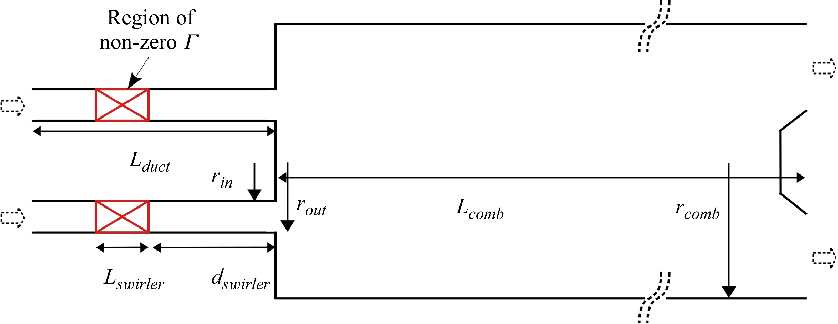


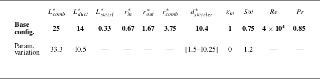


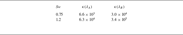


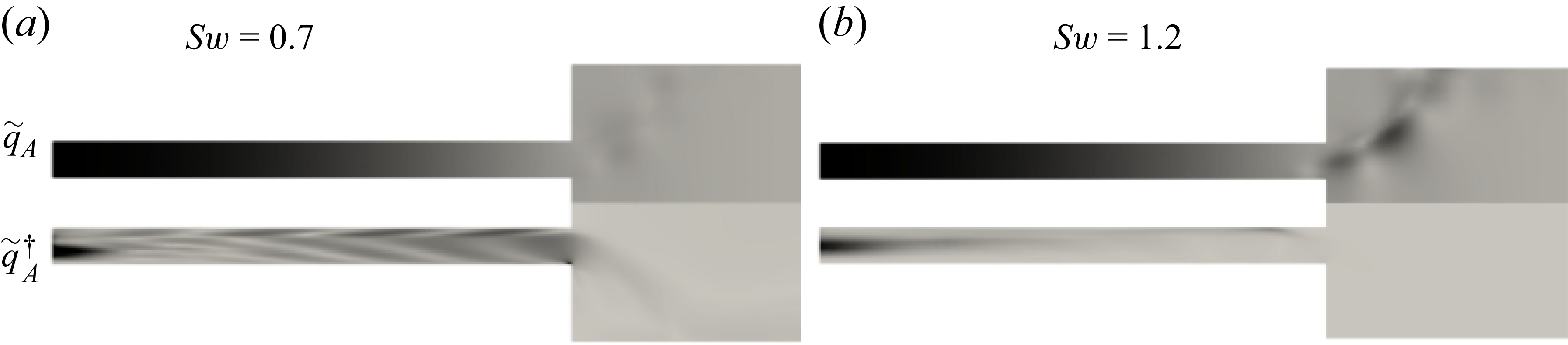


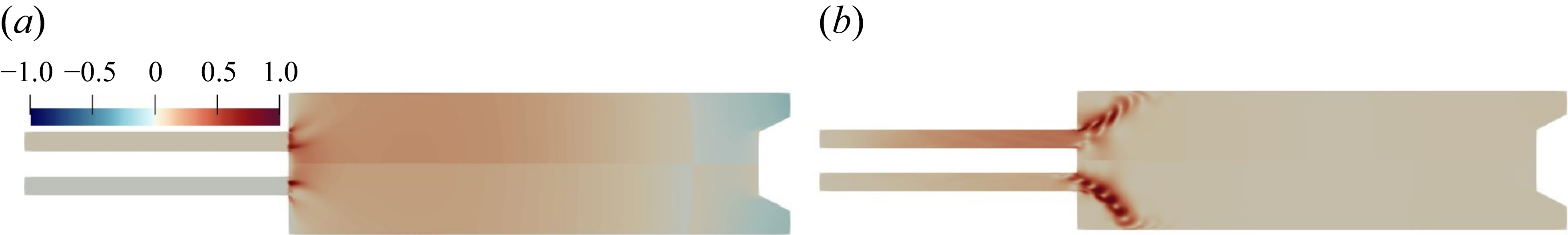


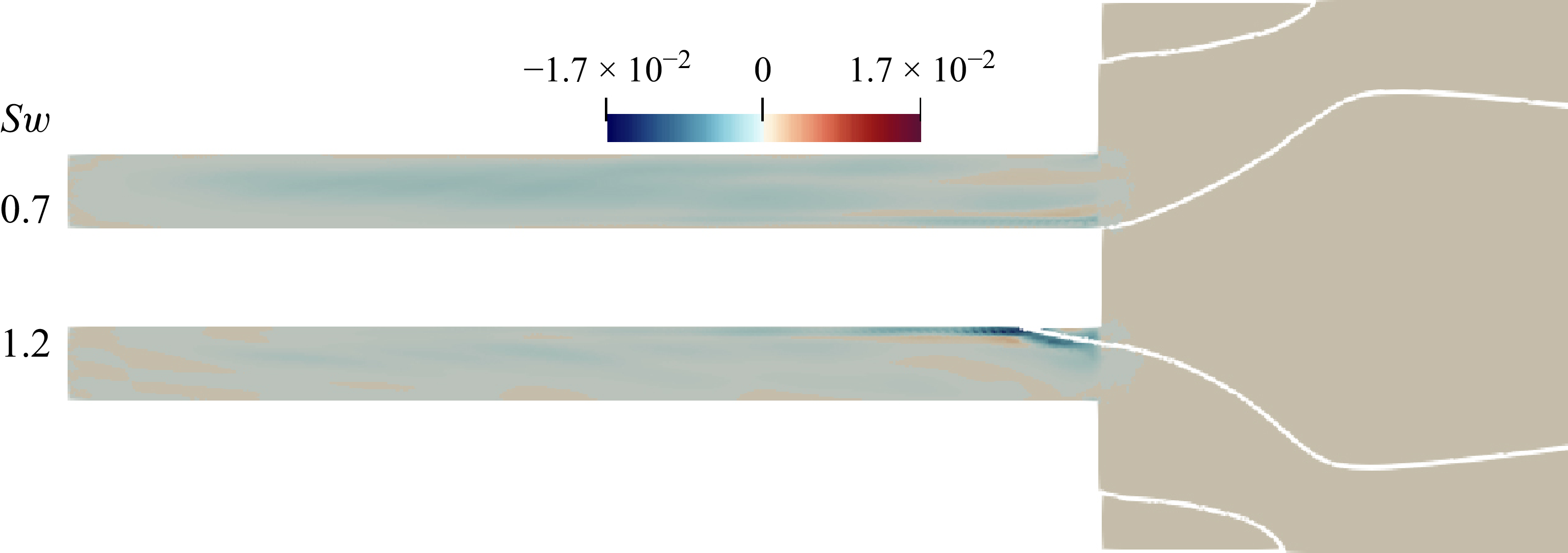
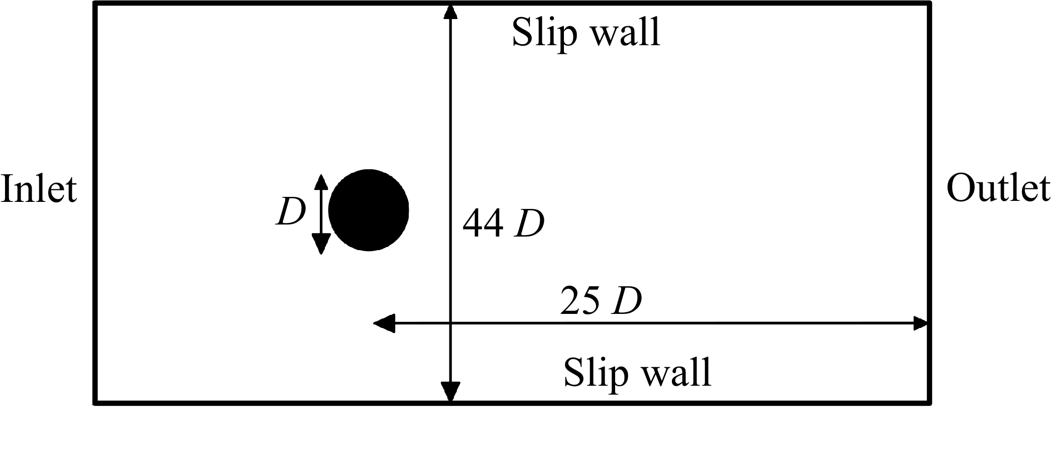


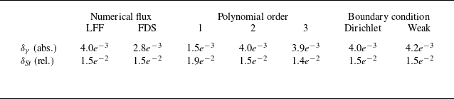


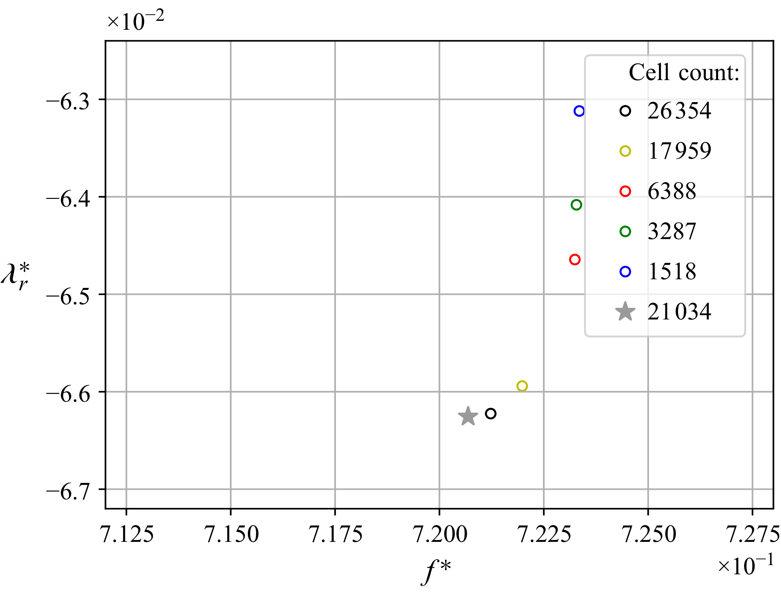


 Open access