





1. Introduction
Understanding how much energy a plasma can release, and how it will be released, is a question that underpins much of plasma physics, from how modern fusion devices will handle/mitigate anomalous transport (e.g. Beidler et al. Reference Beidler2021; Kennedy et al. Reference Kennedy2024), or the nature of turbulent cascades (Schekochihin et al. Reference Schekochihin, Cowley, Dorland, Hammett, Howes, Quataert and Tatsuno2009; Kunz et al. Reference Kunz, Schekochihin, Chen, Abel and Cowley2015), to the creation and persistence of non-thermal distribution functions (Sironi & Spitkovsky Reference Sironi and Spitkovsky2010, Reference Sironi and Spitkovsky2014; Caprioli & Spitkovsky Reference Caprioli and Spitkovsky2014; Werner & Uzdensky Reference Werner and Uzdensky2017; Zhdankin et al. Reference Zhdankin, Werner, Uzdensky and Begelman2017, Reference Zhdankin, Uzdensky, Werner and Begelman2019; Werner & Uzdensky Reference Werner and Uzdensky2021; Zhdankin Reference Zhdankin2021; Uzdensky Reference Uzdensky2022). The simplest way to study the release of such energy is via calculations of linear instability (e.g. Davidson Reference Davidson1981; Gary Reference Gary1993; Hasegawa Reference Hasegawa2012; Ivanov & Adkins Reference Ivanov and Adkins2023; Bott, Cowley & Schekochihin Reference Bott, Cowley and Schekochihin2024). However, this does not, a priori, inform us as to the saturation of the system, and many practical examples concern the nonlinear release of energy from linear stable states (Cowley, Kulsrud & Sudan Reference Cowley, Kulsrud and Sudan1991; Hosking, Wasserman & Cowley Reference Hosking, Wasserman and Cowley2025). Another tractable, and analytically appealing, route towards understanding is to make statements about the total energy budget of the system. This idea has its roots in early work on meteorology, hydrodynamic systems and plasmas (e.g. Lorenz Reference Lorenz1955; Bernstein et al. Reference Bernstein, Frieman, Kruskal and Kulsrud1958; Kruskal & Oberman Reference Kruskal and Oberman1958; Fowler Reference Fowler1963, Reference Fowler1964; Gardner Reference Gardner1963) and has recently received more attention as a method to bound energy release and growth of instabilities in plasmas (Dodin & Fisch Reference Dodin and Fisch2005; Helander Reference Helander2017; Plunk & Helander Reference Plunk and Helander2022).
The root of calculations bounding the released energy, called available energy, stems from two observations; first, the total energy of the system, $E_{\mathrm{tot}}$
, must be conserved and can either be stored in kinetic energy
$E_{\mathrm{tot}}$
, must be conserved and can either be stored in kinetic energy $E_{\mathrm{K}}$
or potential energy
$E_{\mathrm{K}}$
or potential energy $E_{\phi }$
.Footnote
1
Secondly, one is typically able to bound, from below, the kinetic energy of the system by some value
$E_{\phi }$
.Footnote
1
Secondly, one is typically able to bound, from below, the kinetic energy of the system by some value $E_{\mathrm{G}}$
. Together, these observations give the inequality
$E_{\mathrm{G}}$
. Together, these observations give the inequality
 \begin{equation} E_{\phi } = E_{\mathrm{tot}} - E_{\mathrm{K}} \leqslant E_{\mathrm{tot}} - E_{\mathrm{G}} \equiv A_{\mathrm{G}}, \end{equation}
where we define $A_{\mathrm{G}}$
to be the ‘Gardner’ available energy. Of course, the task is now to provide the physical origin of the lower bound on the kinetic energy. This, naturally, arises from entropic considerations: the entropy of the system must increase or stay constant, so all particles cannot conspire to achieve zero velocity (Fowler Reference Fowler1963). This bound can be further upgraded by noting, as Gardner (Reference Gardner1963) did, that when the evolution of the system is well approximated by the mean-field equations, the distribution function
$A_{\mathrm{G}}$
to be the ‘Gardner’ available energy. Of course, the task is now to provide the physical origin of the lower bound on the kinetic energy. This, naturally, arises from entropic considerations: the entropy of the system must increase or stay constant, so all particles cannot conspire to achieve zero velocity (Fowler Reference Fowler1963). This bound can be further upgraded by noting, as Gardner (Reference Gardner1963) did, that when the evolution of the system is well approximated by the mean-field equations, the distribution function $f(\boldsymbol{x},\boldsymbol{v})$
preserves an infinite number of invariants (known as Casimir invariants). These invariants represent the incompressibility of phase space (or equivalently the conservation of level sets of the distribution function) that forbid all particles going to zero velocity. Since Gardner’s work, the concept has been extended in various manners, e.g. allowing for breaking of Casimir invariants through phase-space diffusion (see, e.g. Fisch & Rax Reference Fisch and Rax1993; Kolmes & Fisch Reference Kolmes and Fisch2020; Kolmes, Helander & Fisch Reference Kolmes, Helander and Fisch2020) or by the inclusion of additional adiabatic (e.g. Helander Reference Helander2020; Mackenbach, Proll & Helander Reference Mackenbach, Proll and Helander2022), or symplectic (Qin et al. Reference Qin, Kolmes, Updike, Bohlsen and Fisch2025), invariants.
$f(\boldsymbol{x},\boldsymbol{v})$
preserves an infinite number of invariants (known as Casimir invariants). These invariants represent the incompressibility of phase space (or equivalently the conservation of level sets of the distribution function) that forbid all particles going to zero velocity. Since Gardner’s work, the concept has been extended in various manners, e.g. allowing for breaking of Casimir invariants through phase-space diffusion (see, e.g. Fisch & Rax Reference Fisch and Rax1993; Kolmes & Fisch Reference Kolmes and Fisch2020; Kolmes, Helander & Fisch Reference Kolmes, Helander and Fisch2020) or by the inclusion of additional adiabatic (e.g. Helander Reference Helander2020; Mackenbach, Proll & Helander Reference Mackenbach, Proll and Helander2022), or symplectic (Qin et al. Reference Qin, Kolmes, Updike, Bohlsen and Fisch2025), invariants.
However, the bound on the field energy can not be sharp in general, and this may be understood from the following examples. As first pointed out by Chen (Reference Chen1966a
), a typical calculation of the minimiser of the kinetic energy ignores the fact that the potential energy released is tied fundamentally to the fields, which are themselves supported by the distribution function. Following his logic, it is trivial to show that the bounds derived by Gardner (Reference Gardner1963) are strict (i.e. ‘ $\lt$
’ in (1.1) rather than ‘
$\lt$
’ in (1.1) rather than ‘ $\leqslant$
’). Supposing that the Gardner state is reached, then by energy conservation (1.1) is satisfied with equality
$\leqslant$
’). Supposing that the Gardner state is reached, then by energy conservation (1.1) is satisfied with equality $E_{\phi } = A_{\mathrm{G}}$
. However, this gives an immediate contradiction, since the Gardner state (in the absence of any other conserved quantities) is spatially homogeneous and so has no energy in the fields. Thus, the Gardner state is, in general, inaccessible and the bound (1.1) can never be satisfied with equality. Similarly, Helander (Reference Helander2020) points out that quasineutral plasmas are unable in general to relax to the ground state since the net charge density of the different species needs to sum to zero, restricting the values that the profiles can take on (consequently coupling the species). In ion–electron plasmas in toroidal geometries with adiabatic electrons this is an especially important consideration, as there is no radial particle transport implying that the density profile must be kept fixed. Both of these examples restrict the density profile that the ground state can take on, which can be accounted for by including an arbitrary density profile in the ground state. That, precisely, is the goal of this paper: to find general expressions of a ground state with a given density profile. The density profile is thereupon coupled to, e.g. the field equations, lowering the available energy.
$E_{\phi } = A_{\mathrm{G}}$
. However, this gives an immediate contradiction, since the Gardner state (in the absence of any other conserved quantities) is spatially homogeneous and so has no energy in the fields. Thus, the Gardner state is, in general, inaccessible and the bound (1.1) can never be satisfied with equality. Similarly, Helander (Reference Helander2020) points out that quasineutral plasmas are unable in general to relax to the ground state since the net charge density of the different species needs to sum to zero, restricting the values that the profiles can take on (consequently coupling the species). In ion–electron plasmas in toroidal geometries with adiabatic electrons this is an especially important consideration, as there is no radial particle transport implying that the density profile must be kept fixed. Both of these examples restrict the density profile that the ground state can take on, which can be accounted for by including an arbitrary density profile in the ground state. That, precisely, is the goal of this paper: to find general expressions of a ground state with a given density profile. The density profile is thereupon coupled to, e.g. the field equations, lowering the available energy.
A few comments are warranted about the applicability of this framework. If the system is thermodynamically closed rather than isolated, the thermal energy released can evidently be carried away by, e.g. radiation, and the Gardner state may be achieved. Similarly, even if the system is isolated, it may be possible to release energy in a form that only weakly interacts with the plasma (e.g. in high-frequency photons) in which case the Gardner state is also (asymptotically) realisable. We disregard such cases in this investigation and focus on scenarios where the kinetic energy released by the plasma retains a strong coupling to it (as is typical in low-frequency closures of the electromagnetic equations). There is a further issue linking available energy, be it accessible or not, to turbulence. Part of the turbulent energy in the plasma may reside in, e.g. mean flows or temperature fluctuations, and is thus not solely in the electric field. More generally, the relationship between turbulence and available energy will depend on the type of turbulence driven. The current focus on the electric field makes this investigation relevant for electrostatic turbulence, and acts as a stepping stone to more general (e.g. electromagnetic) cases.
The rest of this paper is as follows. In § 2 we briefly review the problem of ground states in collisionless plasmas and establish the formalism for finding self-consistent ground states. This formalism is rooted in the functional optimisation approach codified in Helander (Reference Helander2017) where constraints on the density profiles are included. This can be computed perturbatively when the system is close to its ground state, as done in § 4. However, to avoid the immediate notational clutter that comes with generality and to gain insight into situations that fall outside of the asymptotic framework, in § 3 we work through the theory for the simplest possible plasma: electrons with a model distribution function (a ‘single-waterbag’ distribution), in presence of an electrostatic potential alone and a fixed background of ions. We find that a self-consistent ground state (i.e. one that supports an electric field with an energy equal to the available energy) will, in such plasmas, naturally seek to hold the electric-field fluctuations in the longest wavelength modes: from an energetic point of view, electrons wish to create modes that will influence ions. Indeed, we will find this to be precisely true by including the effect of screening on scales larger than the Debye length, and the self-consistent ground state instead seeks fluctuations that are on the scale of the Debye length. In § 3.4 we verify the bounds we derive using particle-in-cell (PIC) simulations in one dimension. In § 5 we summarise our arguments and present possible future avenues of research.
2. Theory
We first review the basic theory of ground states in collisionless plasmas. In Helander (Reference Helander2017), ground state and available energy calculations are posed as constrained functional optimisation problems. Of specific interest is the following: suppose that the dynamics of a distribution function $f$
are well described by a collisionless Boltzmann equation. Furthermore, splitting phase space
$f$
are well described by a collisionless Boltzmann equation. Furthermore, splitting phase space $\boldsymbol{x}=(\boldsymbol{r},\boldsymbol{v})$
into invariant coordinates
$\boldsymbol{x}=(\boldsymbol{r},\boldsymbol{v})$
into invariant coordinates $\boldsymbol{y}$
, and remaining coordinates
$\boldsymbol{y}$
, and remaining coordinates $\boldsymbol{z}$
,Footnote
2
with the Jacobian
$\boldsymbol{z}$
,Footnote
2
with the Jacobian $\mathrm{d} \boldsymbol{x} = \mathrm{d} \boldsymbol{r}\mathrm{d}\boldsymbol{v} = \sqrt {g(\boldsymbol{y},\boldsymbol{z})} \; \mathrm{d} \boldsymbol{y} \mathrm{d} \boldsymbol{z}$
, the dynamical system becomes
$\mathrm{d} \boldsymbol{x} = \mathrm{d} \boldsymbol{r}\mathrm{d}\boldsymbol{v} = \sqrt {g(\boldsymbol{y},\boldsymbol{z})} \; \mathrm{d} \boldsymbol{y} \mathrm{d} \boldsymbol{z}$
, the dynamical system becomes
 \begin{equation} \frac {\mathrm{d} (f \sqrt {g})}{\mathrm{d} t} = \frac {\partial (f \sqrt {g})}{\partial t} + \boldsymbol{\dot {z}} \boldsymbol{\cdot }\frac {\partial (f \sqrt {g})}{\partial \boldsymbol{z}} = 0, \end{equation}
where the term involving $\boldsymbol{\dot {y}}$
is equal to zero as a consequence of its invariance. Due to the incompressibility of phase space,
$\boldsymbol{\dot {y}}$
is equal to zero as a consequence of its invariance. Due to the incompressibility of phase space, $\mathrm{d} \sqrt {g} / \mathrm{d} t = 0$
, (2.1) has an infinite number of invariants, often called the Casimir invariants, equivalent to the conservation of phase volume in which the phase-space density exceeds a particular value
$\mathrm{d} \sqrt {g} / \mathrm{d} t = 0$
, (2.1) has an infinite number of invariants, often called the Casimir invariants, equivalent to the conservation of phase volume in which the phase-space density exceeds a particular value $\eta$
, viz.,
$\eta$
, viz.,
 \begin{equation} H[f;\eta ,\boldsymbol{y}] = \int \mathrm{d}{\boldsymbol{z}}\, \varTheta [ f(t,\boldsymbol{y},\boldsymbol{z}) - \eta ] \sqrt {g}, \qquad \frac {\mathrm{d}H}{\mathrm{d}t} = 0 ,\end{equation}
where $\varTheta (x)$
is the Heaviside function. These constraints imply that the measure of the level sets of
$\varTheta (x)$
is the Heaviside function. These constraints imply that the measure of the level sets of $f$
are constant in time for each combination of invariants
$f$
are constant in time for each combination of invariants $\boldsymbol{y}$
. The ground state is now defined as the distribution that minimises the kinetic energy of the plasma,
$\boldsymbol{y}$
. The ground state is now defined as the distribution that minimises the kinetic energy of the plasma, $E_K[f] \equiv \int \mathrm{d}{\boldsymbol{x}} \epsilon f$
, with
$E_K[f] \equiv \int \mathrm{d}{\boldsymbol{x}} \epsilon f$
, with $\epsilon$
being the particle’s kinetic energy, subject to Casimir invariants captured by (2.2). However, anticipating the need to enforce realisability of this state, we also enforce that the density has a certain prescribed profile,
$\epsilon$
being the particle’s kinetic energy, subject to Casimir invariants captured by (2.2). However, anticipating the need to enforce realisability of this state, we also enforce that the density has a certain prescribed profile,
 \begin{equation} \int \mathrm{d}{\boldsymbol{v}} f = n(\boldsymbol{r}). \end{equation}
To enforce the constraints ((2.2), (2.3)) while minimising the total energy, one must minimise the functional
 \begin{align} W[f] = & \int \mathrm{d}{\boldsymbol{z}}\, \mathrm{d}{\boldsymbol{y}}\, \epsilon f \sqrt {g} + \left ( \int \mathrm{d}{\boldsymbol{z}}\, \mathrm{d}{\boldsymbol{y}} \kappa (\boldsymbol{r}) f \sqrt {g} - \int \mathrm{d}{\boldsymbol{r}}\, \kappa (\boldsymbol{r}) n(\boldsymbol{r}) \right )\nonumber \\ & +\int \mathrm{d}{\eta }\, \lambda (\eta ;\boldsymbol{y}) \left ( \int \mathrm{d}{\boldsymbol{z}}\, \varTheta [ f - \eta ] \sqrt {g} - \int \mathrm{d}{\boldsymbol{z}}\, \varTheta [ f(t=0) - \eta ] \sqrt {g} \right )\end{align}
unconditionally with respect to the distribution function $f$
and the Lagrange multipliers
$f$
and the Lagrange multipliers $\kappa$
and
$\kappa$
and $\lambda$
. These two Lagrange multipliers enforce the ground-state density and Casimir invariants, respectively. Writing
$\lambda$
. These two Lagrange multipliers enforce the ground-state density and Casimir invariants, respectively. Writing $f = F + \delta f$
and taking the first variation, one finds that
$f = F + \delta f$
and taking the first variation, one finds that
 \begin{equation} \int \mathrm{d}{\boldsymbol{z}} \left [ \lambda (F,\boldsymbol{y}) + \epsilon + \kappa \right ] \delta f \sqrt {g} = 0 \implies F = F[\epsilon (\boldsymbol{x})+\kappa (\boldsymbol{r});\boldsymbol{y}]. \end{equation}
By taking the second variation and imposing that it is positive definite, one finds that
 \begin{equation} \frac {\partial F(w,\boldsymbol{y})}{\partial w} \leqslant 0. \end{equation}
Next, noting that the Casimirs of the initial distribution function and the ground state must be equal, one finds that $\int \mathrm{d}{\boldsymbol{z}}\, \varTheta [f(t=0) - \eta ]\sqrt {g} = \int \mathrm{d}{\boldsymbol{z}}\, \varTheta [F - \eta ]\sqrt {g}$
, and applying the inverse of
$\int \mathrm{d}{\boldsymbol{z}}\, \varTheta [f(t=0) - \eta ]\sqrt {g} = \int \mathrm{d}{\boldsymbol{z}}\, \varTheta [F - \eta ]\sqrt {g}$
, and applying the inverse of $F$
to the argument on the right-hand side gives
$F$
to the argument on the right-hand side gives
 \begin{equation} \int \mathrm{d}{\boldsymbol{z}}\, \varTheta [f(t=0) - F(w,\boldsymbol{y})] \sqrt {g} = \int \mathrm{d}{\boldsymbol{z}}\, \varTheta [w - \epsilon - \kappa ] \sqrt {g}, \end{equation}
having defined $\eta \equiv F(w,\boldsymbol{y})$
. This is a nonlinear integral equation for
$\eta \equiv F(w,\boldsymbol{y})$
. This is a nonlinear integral equation for $F[\epsilon (\boldsymbol{x})+\kappa (\boldsymbol{r}),\boldsymbol{y}]$
, where the Lagrange multiplier
$F[\epsilon (\boldsymbol{x})+\kappa (\boldsymbol{r}),\boldsymbol{y}]$
, where the Lagrange multiplier $\kappa (\boldsymbol{r})$
is determined by the condition
$\kappa (\boldsymbol{r})$
is determined by the condition
 \begin{equation} \int \mathrm{d}{\boldsymbol{v}} F[\epsilon +\kappa (\boldsymbol{r});\boldsymbol{y}] = n(\boldsymbol{r}). \end{equation}
Equations (2.7) and (2.8) together give the ground state in terms of some initial distribution $f_i$
and ground-state density profile
$f_i$
and ground-state density profile $n(\boldsymbol{r})$
. The available energy, for a system with a given ground-state density profile, is then
$n(\boldsymbol{r})$
. The available energy, for a system with a given ground-state density profile, is then
 \begin{align} A[f_i(\boldsymbol{x}),n(\boldsymbol{r});\boldsymbol{y}] &= \int \mathrm{d}{\boldsymbol{x}} f_i(\boldsymbol{x}) \epsilon - \int \mathrm{d}{\boldsymbol{x}} F[\epsilon +\kappa ; \boldsymbol{y}] \epsilon . \end{align}
This expression gives the available energy subject to an explicit density constraint, and by coupling it to additional relevant equations one can calculate the ‘accessible’ available energy. Relaxing the constraint on the density ( $\kappa (\boldsymbol{r}) = 0$
) recovers the Gardner (Reference Gardner1963) bound, whose corresponding ground state we will refer to as the ‘Gardner state’. In practice it is often the case that the density is only constrained via its implicit relation to other fields (e.g. Poisson’s equation or the gyrokinetic field equations), itself dependent on the liberated energy, so that the available energy is described by an implicit relationship. We illustrate the simplest example of this in the next section.
$\kappa (\boldsymbol{r}) = 0$
) recovers the Gardner (Reference Gardner1963) bound, whose corresponding ground state we will refer to as the ‘Gardner state’. In practice it is often the case that the density is only constrained via its implicit relation to other fields (e.g. Poisson’s equation or the gyrokinetic field equations), itself dependent on the liberated energy, so that the available energy is described by an implicit relationship. We illustrate the simplest example of this in the next section.
3. Single-waterbag ground state
3.1. The set-up
Let us consider the simplest possible example in which to compute the available energy $A$
with no invariant coordinates (
$A$
with no invariant coordinates ( $\boldsymbol{y} = \varnothing$
): an electrostatic plasma consisting of a single species, similar to Chen (Reference Chen1966a
). The potential energy of such a system is
$\boldsymbol{y} = \varnothing$
): an electrostatic plasma consisting of a single species, similar to Chen (Reference Chen1966a
). The potential energy of such a system is
 \begin{equation} E_{\phi } = \int \mathrm{d}{\boldsymbol{r}}\, \frac {|\boldsymbol{\nabla }\phi |^{2}}{8\pi }, \end{equation}
where the electrostatic potential $\phi$
is related to density fluctuations
$\phi$
is related to density fluctuations $\delta n_e$
by Poisson’s equation,
$\delta n_e$
by Poisson’s equation, $\boldsymbol{\nabla} ^2 \phi \propto \delta n_e$
, or quasineutrality
$\boldsymbol{\nabla} ^2 \phi \propto \delta n_e$
, or quasineutrality $\phi \propto \delta n_e$
. To make progress in solving (2.7), we assume that the initial distribution function
$\phi \propto \delta n_e$
. To make progress in solving (2.7), we assume that the initial distribution function $f(t=0)$
consists of a single waterbag: a distribution that can take on only two values;
$f(t=0)$
consists of a single waterbag: a distribution that can take on only two values; $\eta$
or zero. Under such conditions, the generally infinite number of Casimir invariants reduce to a single constraint for the simple reason that there is only a single level set (i.e. phase-volume conservation becomes equivalent to particle-number conservation; Kadomtsev & Pogutse Reference Kadomtsev and Pogutse1970; Ewart et al. Reference Ewart, Brown, Adkins and Schekochihin2022).
$\eta$
or zero. Under such conditions, the generally infinite number of Casimir invariants reduce to a single constraint for the simple reason that there is only a single level set (i.e. phase-volume conservation becomes equivalent to particle-number conservation; Kadomtsev & Pogutse Reference Kadomtsev and Pogutse1970; Ewart et al. Reference Ewart, Brown, Adkins and Schekochihin2022).
Consider for the sake of illustration the case depicted in figure 1. It should be evident that the Gardner ground state will collapse to the lowest velocity coordinate, whilst maintaining its total volume to satisfy incompressibility. In reality such a system will release its energy into electrostatic fluctuations, coupled to the density fluctuations, which forbid the system from reaching this state. Imposing that the ground state has some spatial density variation, $n(\boldsymbol{r})$
, will result in this ground state having a varying thermal width to accommodate the density variation (which will be symmetric about
$n(\boldsymbol{r})$
, will result in this ground state having a varying thermal width to accommodate the density variation (which will be symmetric about $v_{x}=0$
to minimise kinetic energy). Such considerations carry over to arbitrary dimensions: the ground state will collapse onto a sphere around
$v_{x}=0$
to minimise kinetic energy). Such considerations carry over to arbitrary dimensions: the ground state will collapse onto a sphere around $\boldsymbol{v} = 0$
(since the isocontours of particle energy are spheres), whose radius may vary spatially in order to support density variations. Expressing (2.5) in a convenient form (which in the case of the waterbag is either
$\boldsymbol{v} = 0$
(since the isocontours of particle energy are spheres), whose radius may vary spatially in order to support density variations. Expressing (2.5) in a convenient form (which in the case of the waterbag is either $\eta$
or zero, as captured by a Heaviside function), we thus have
$\eta$
or zero, as captured by a Heaviside function), we thus have
 \begin{equation} F\left [\frac {1}{2}m|\boldsymbol{v}|^{2} + \kappa (\boldsymbol{r}) \right ] = \eta \varTheta [ a(\boldsymbol{r})^2 - |\boldsymbol{v}|^{2}], \end{equation}
where $a(\boldsymbol{r})$
is chosen such that
$a(\boldsymbol{r})$
is chosen such that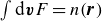 $\int \mathrm{d}{\boldsymbol{v}} F = n(\boldsymbol{r})$
, i.e.
$\int \mathrm{d}{\boldsymbol{v}} F = n(\boldsymbol{r})$
, i.e.
 \begin{equation} a(\boldsymbol{r}) = \frac {1}{\sqrt {\pi }}\left [\varGamma \left (1 + \frac {d}{2}\right ) \frac {n(\boldsymbol{r})}{\eta }\right ]^{1/d}, \end{equation}
where the gamma function $\varGamma (x) = (x-1)!$
has emerged to give an expression for the volumes of a ball in
$\varGamma (x) = (x-1)!$
has emerged to give an expression for the volumes of a ball in $d$
dimensions. The constrained ground state now readily gives the system’s kinetic energy
$d$
dimensions. The constrained ground state now readily gives the system’s kinetic energy
 \begin{equation} E_{\mathrm{K}} \geqslant \iint \mathrm{d}{\boldsymbol{r}}\mathrm{d}{\boldsymbol{v}}\frac {1}{2}m|\boldsymbol{v}|^{2}F = E_{\mathrm{G}} \left \langle \left [\frac {n(\boldsymbol{r})}{n_{0}} \right ]^{({d+2})/{d}} \right \rangle , \end{equation}
where $\langle \ldots \rangle \equiv \int \mathrm{d}{\boldsymbol{r}} \ldots / V$
is a volume average (
$\langle \ldots \rangle \equiv \int \mathrm{d}{\boldsymbol{r}} \ldots / V$
is a volume average ( $V$
being the system’s volume), and the ground-state energy with an unconstrained density profile (
$V$
being the system’s volume), and the ground-state energy with an unconstrained density profile ( $\kappa =0$
),
$\kappa =0$
), $E_{\mathrm{G}}$
, is given as
$E_{\mathrm{G}}$
, is given as
 \begin{equation} E_{\mathrm{G}} = \frac {mV}{ \pi \eta ^{2/d} (2+d)\varGamma \left ({d}/{2}\right )} \left [ \varGamma \left ( 1 + \frac {d}{2} \right ) n_0 \right ]^{({d+2})/{d}}. \end{equation}
While (3.4) is specific to the single-waterbag model it serves to analytically illustrate the cost of a density perturbation: in order to conserve phase-space volume while enhancing density, more particles must be elevated to larger velocities, which costs more energy.
A schematic showing the distinction between the Gardner state and an accessible ground state. In the leftmost panel we show a possible initial condition with energy available (the two-stream instability); its Gardner state (without a constraint on the density), $F_{\mathrm{G}}$
, is given in the middle panel, and it may be seen that it is spatially homogenous. However, in order to support an electric field containing the energy released by the instability, the ground state must have spatial variation, and an example of such a spatially varying ground state,
$F_{\mathrm{G}}$
, is given in the middle panel, and it may be seen that it is spatially homogenous. However, in order to support an electric field containing the energy released by the instability, the ground state must have spatial variation, and an example of such a spatially varying ground state, $F$
, is given in the rightmost panel.
$F$
, is given in the rightmost panel.

Figure 1. Long description
The image consists of three panels side by side, each depicting a different state of a plasma system. The leftmost panel shows an initial condition with energy available, specifically illustrating the two-stream instability. This panel features two horizontal shaded regions centered around positive and negative velocities. The middle panel represents the Gardner state without a constraint on the density. This state is spatially homogeneous, as indicated by the uniform shading across the entire panel. The rightmost panel shows an example of a spatially varying ground state, which is necessary to support an electric field containing the energy released by the instability. This panel features a wavy, non-uniform shading, indicating spatial variation. The x-axis in all panels ranges from negative pi to positive pi, and the y-axis ranges from negative v0 to positive v0, representing velocity. The panels collectively illustrate the mappin from ant initial state with available energy to a spatially homogeneous Gardner state and to a spatially varying ground state to support the released energy.
The Gardner bound is given as $A_{\mathrm{G}} = E_{\mathrm{init}} - E_{\mathrm{G}}$
, so that the available energy subject to a density perturbation is
$A_{\mathrm{G}} = E_{\mathrm{init}} - E_{\mathrm{G}}$
, so that the available energy subject to a density perturbation is
 \begin{equation} A = A_{\mathrm{G}} - E_{\mathrm{G}}\langle [1 + \nu (\boldsymbol{r}) ]^{({d+2})/{d}} - 1 \rangle , \end{equation}
where we have set $n(\boldsymbol{r}) = n_0[1+\nu (\boldsymbol{r})]$
. Of course, all this energy must be stored in the energy of the fields
$n(\boldsymbol{r}) = n_0[1+\nu (\boldsymbol{r})]$
. Of course, all this energy must be stored in the energy of the fields $E_{\phi }$
which, for an electrostatic plasma, gives the condition
$E_{\phi }$
which, for an electrostatic plasma, gives the condition
 \begin{equation} E_{\mathrm{\phi }}[\nu (\boldsymbol{r})] = \int \mathrm{d}{\boldsymbol{r}}\,\frac {|\boldsymbol{\nabla }\phi |^{2}}{8\pi } = A_{\mathrm{G}} - E_{\mathrm{G}}\langle [1 + \nu (\boldsymbol{r}) ]^{({d+2})/{d}} -1 \rangle , \end{equation}
where $\phi [\nu (\boldsymbol{r})]$
. Note that there are two additional constraints: one to conserve the total number of particles,
$\phi [\nu (\boldsymbol{r})]$
. Note that there are two additional constraints: one to conserve the total number of particles, $\int \mathrm{d}{\boldsymbol{r}} \nu = 0$
, and one to have positive number density, namely
$\int \mathrm{d}{\boldsymbol{r}} \nu = 0$
, and one to have positive number density, namely $\nu (\boldsymbol{r}) \geqslant -1, \ \text{for all }\boldsymbol{r}$
. In order to close these equations one needs to specify how
$\nu (\boldsymbol{r}) \geqslant -1, \ \text{for all }\boldsymbol{r}$
. In order to close these equations one needs to specify how $\phi$
and
$\phi$
and $\nu$
are related. For a fixed background of ions, the relationship is simply
$\nu$
are related. For a fixed background of ions, the relationship is simply
 \begin{equation} -\lambda _{D,{\mathrm{ref}}}^2 \boldsymbol{\nabla} ^2 \hat {\phi } = \nu , \end{equation}
where we have introduced the Debye length $\lambda _{D,{\mathrm{s}}} = \sqrt {T_{\mathrm{s}}/4\pi \mathrm{e}^2 n_0}$
as a reference length scale, and the electric potential is normalised as
$\lambda _{D,{\mathrm{s}}} = \sqrt {T_{\mathrm{s}}/4\pi \mathrm{e}^2 n_0}$
as a reference length scale, and the electric potential is normalised as $\hat {\phi } = \mathrm{e} \phi /T_{\mathrm{ref}}$
, where
$\hat {\phi } = \mathrm{e} \phi /T_{\mathrm{ref}}$
, where $T_{\mathrm{ref}}$
is some reference temperature (here an appropriate choice would be, e.g.
$T_{\mathrm{ref}}$
is some reference temperature (here an appropriate choice would be, e.g. $T_{\mathrm{ref}} \propto E_{\mathrm{G}}$
). Equations (3.7) and (3.8) now constitute an implicit relation for the density constraint
$T_{\mathrm{ref}} \propto E_{\mathrm{G}}$
). Equations (3.7) and (3.8) now constitute an implicit relation for the density constraint $\nu (\boldsymbol{x})$
. Before solving them, it is instructive to quickly arrive at an intuitive result. Letting the density (and thus potential) be non-zero only at some predefined wavenumber,
$\nu (\boldsymbol{x})$
. Before solving them, it is instructive to quickly arrive at an intuitive result. Letting the density (and thus potential) be non-zero only at some predefined wavenumber, $k_0$
, gives a field energy, via (3.7) and (3.8), that scales as
$k_0$
, gives a field energy, via (3.7) and (3.8), that scales as $E_\phi \propto k_0^2 \phi _k^2 \propto \nu _{k}/k_0^2$
. Assuming the fluctuations are small, the available energy (3.6) becomes
$E_\phi \propto k_0^2 \phi _k^2 \propto \nu _{k}/k_0^2$
. Assuming the fluctuations are small, the available energy (3.6) becomes $A \approx A_{\mathrm{G}} - C \nu _k^2$
, where
$A \approx A_{\mathrm{G}} - C \nu _k^2$
, where $C$
is some positive constant. By equating
$C$
is some positive constant. By equating $A$
to
$A$
to $E_\phi$
we see that
$E_\phi$
we see that $E_\phi =A$
is possible in the limit
$E_\phi =A$
is possible in the limit $k_0 \rightarrow 0$
: purely electrostatic fluctuations maximise their released energy by producing the large-scale modes (i.e. long wavelengths can store large amounts of potential energy with relatively little density perturbation). For neutralising backgrounds, then, the Gardner bound is always attainable unless the lowest accessible wavenumber is non-zero (although whether this mode is dynamically activated is not answered by this framework).
$k_0 \rightarrow 0$
: purely electrostatic fluctuations maximise their released energy by producing the large-scale modes (i.e. long wavelengths can store large amounts of potential energy with relatively little density perturbation). For neutralising backgrounds, then, the Gardner bound is always attainable unless the lowest accessible wavenumber is non-zero (although whether this mode is dynamically activated is not answered by this framework).
However, the appearance of structures much larger than the Debye length is at odds with the assumption of a static background, as for sufficiently long wavelengths (i.e. longer than the Debye length) the electric field is shielded. With two species, Poisson’s equation becomes
 \begin{equation} -\lambda _{D,{\mathrm{bg}}}^2 \boldsymbol{\nabla} ^2 \hat {\phi } = \nu - \nu _{\mathrm{bg}}, \end{equation}
where the subscript ‘bg’ refers to a background species. Assume this species has a Boltzmann response $\nu _{\mathrm{bg}} = B ( \exp [\hat {\phi }] -1 )$
, having set
$\nu _{\mathrm{bg}} = B ( \exp [\hat {\phi }] -1 )$
, having set $T_{\mathrm{ref}} = T_{\mathrm{bg}}$
, which is the temperature associated with the background. The potential is described by the Poisson–Boltzmann equation
$T_{\mathrm{ref}} = T_{\mathrm{bg}}$
, which is the temperature associated with the background. The potential is described by the Poisson–Boltzmann equation
 \begin{equation} - \lambda _{D,{\mathrm{bg}}}^2 \boldsymbol{\nabla} ^2 \hat {\phi } + B ({\rm e}^{\hat {\phi }} -1 ) = \nu , \end{equation}
where $B \in [0,1]$
is the parameter that controls if the background is fully neutralising (
$B \in [0,1]$
is the parameter that controls if the background is fully neutralising ( $B=0$
) or adheres to the Boltzmann distribution (
$B=0$
) or adheres to the Boltzmann distribution ( $B=1$
), introduced so that both cases are captured in the calculation that follows.Footnote
3
The Boltzmann response introduces an additional effect that should be accounted for: if
$B=1$
), introduced so that both cases are captured in the calculation that follows.Footnote
3
The Boltzmann response introduces an additional effect that should be accounted for: if $B=1$
, the background species will inherit the perturbations of
$B=1$
, the background species will inherit the perturbations of $\nu$
, which brings an associated energetic cost. Assuming this energetic cost scales like the waterbag solution, it may be set to
$\nu$
, which brings an associated energetic cost. Assuming this energetic cost scales like the waterbag solution, it may be set to $A_{\mathrm{bg}} = - E_{\mathrm{bg}} \langle [1 +\nu _{\mathrm{bg}}]^{({d+2})/{d}} - 1 \rangle ,$
where we have assumed that the background has no free energy in its initial state (i.e. the background does not contribute to
$A_{\mathrm{bg}} = - E_{\mathrm{bg}} \langle [1 +\nu _{\mathrm{bg}}]^{({d+2})/{d}} - 1 \rangle ,$
where we have assumed that the background has no free energy in its initial state (i.e. the background does not contribute to $A_{\mathrm{G}}$
).Footnote
4
The total available energy is now the sum of the two species, resulting in
$A_{\mathrm{G}}$
).Footnote
4
The total available energy is now the sum of the two species, resulting in
 \begin{equation} A = A_{\mathrm{G}} - E_{\mathrm{G}}\big\langle [1 + \nu ]^{({d+2})/{d}} - 1 \big\rangle - E_{\mathrm{bg}} \big\langle [1 + \nu _{\mathrm{bg}} ]^{({d+2})/{d}} - 1 \big\rangle . \end{equation}
Our task is to maximise this available energy, subject to $A = E_\phi$
and a positive number density. In general, these equations do not permit analytical solutions, but they may be solved perturbatively when the initial condition is close to the ground state, and scalings may be derived when it is very far from it.
$A = E_\phi$
and a positive number density. In general, these equations do not permit analytical solutions, but they may be solved perturbatively when the initial condition is close to the ground state, and scalings may be derived when it is very far from it.
3.2. Limit of small ground-state density fluctuations
Let $|\nu |^2 \sim |\nu _{\mathrm{bg}}|^2 \sim A_{\mathrm{G}}/E_{\mathrm{G}}\ll 1$
and, in order to preserve the number of particles, we set
$|\nu |^2 \sim |\nu _{\mathrm{bg}}|^2 \sim A_{\mathrm{G}}/E_{\mathrm{G}}\ll 1$
and, in order to preserve the number of particles, we set $\int \mathrm{d}{\boldsymbol{r}} \nu = 0$
. Taylor expanding the Poisson–Boltzmann equation and taking its Fourier transform results in
$\int \mathrm{d}{\boldsymbol{r}} \nu = 0$
. Taylor expanding the Poisson–Boltzmann equation and taking its Fourier transform results in
 \begin{equation} \big(\lambda _{D,{\mathrm{bg}}}^2 k^2 + B \big) \hat {\phi }_{\boldsymbol{k}} = \nu _{\boldsymbol{k}}, \end{equation}
where the subscript $\boldsymbol{k}$
denotes the
$\boldsymbol{k}$
denotes the $\boldsymbol{k}$
th spectral component (e.g.
$\boldsymbol{k}$
th spectral component (e.g. $\nu (\boldsymbol{r}) = \int \mathrm{d}{\boldsymbol{k}} \nu _{\boldsymbol{k}} {\rm e}^{\mathrm{i} \boldsymbol{k} \boldsymbol{\cdot }\boldsymbol{r}}$
). Expanding (3.11), invoking Plancherel’s theorem, and employing Poisson’s equation gives
$\nu (\boldsymbol{r}) = \int \mathrm{d}{\boldsymbol{k}} \nu _{\boldsymbol{k}} {\rm e}^{\mathrm{i} \boldsymbol{k} \boldsymbol{\cdot }\boldsymbol{r}}$
). Expanding (3.11), invoking Plancherel’s theorem, and employing Poisson’s equation gives
 \begin{equation} A = A_{\mathrm{G}} - \frac {d+2}{d^2} \frac {(2 \pi )^d}{V} \int \mathrm{d}{\boldsymbol{k}}\, |\nu _{\boldsymbol{k}}|^2 \left (E_{\mathrm{G}} + E_{\mathrm{bg}} \frac {B^2}{\big(B+\lambda _{D,{\mathrm{bg}}}^2 k^2\big)^2}\right )\!. \end{equation}
Similarly manipulating the field energy yields
 \begin{equation} E_{\phi } = E_{\phi ,0} \frac {(2 \pi )^d}{V} \int \mathrm{d}{\boldsymbol{k}}\, \frac { \lambda _{D,{\mathrm{bg}}}^2 k^2 |\nu _{\boldsymbol{k}} | ^2}{\big(B + \lambda _{D,{\mathrm{bg}}}^2 k^2 \big)^2}, \end{equation}
where $E_{\phi ,0} = V n_0 T_{\mathrm{bg}}/2$
. Equating these expressions,
$E_{\phi ,0} = V n_0 T_{\mathrm{bg}}/2$
. Equating these expressions, $A=E_\phi$
, is equivalent to
$A=E_\phi$
, is equivalent to
 \begin{equation} \int \mathrm{d}{\boldsymbol{k}}\, \frac {(2\pi )^d|\nu _{\boldsymbol{k}}|^2}{V A_{\mathrm{G}}} \left [ E_{\phi ,0} \frac { \lambda _{D,{\mathrm{bg}}}^2 k^2 }{\left (B + \lambda _{D,{\mathrm{bg}}}^2 k^2 \right )^2} + E_{\mathrm{G}} \frac {d+2}{d^2} + E_{\mathrm{bg}} \frac {d+2}{d^2} \frac {B^2}{\big(B+ \lambda _{D,{\mathrm{bg}}}^2 k^2\big)^2} \right ] = 1, \end{equation}
and defining the integrand of (3.15) to be the distribution $\upsilon (\boldsymbol{k})$
with unit density automatically satisfies the equation. The field energy may now be expressed as
$\upsilon (\boldsymbol{k})$
with unit density automatically satisfies the equation. The field energy may now be expressed as
 \begin{equation} E_{\phi } = A_{\mathrm{G}}\! \int\! \mathrm{d}{\boldsymbol{k}}\, \upsilon (\boldsymbol{k}) \frac {E_{\phi ,0} \lambda _{D,{\mathrm{bg}}}^2 k^2 }{E_{\phi ,0} \lambda _{D,{\mathrm{bg}}}^2 k^2 + E_{\mathrm{G}} (({d+2})/{d^2}) \big(B+\lambda _{D,{\mathrm{bg}}}^2 k^2\big)^2 + B^2 E_{\mathrm{bg}} (({d+2})/{d^2})}, \end{equation}
and this quantity is maximised by letting $\upsilon (\boldsymbol{k})$
be a Dirac-delta distribution, non-zero at a wavenumber that maximises the fraction. This optimal wavenumber is given as
$\upsilon (\boldsymbol{k})$
be a Dirac-delta distribution, non-zero at a wavenumber that maximises the fraction. This optimal wavenumber is given as
 \begin{equation} \lambda _{D,{\mathrm{bg}}}^2 k_0^2 = B \sqrt {1 + \frac {E_{\mathrm{bg}}}{E_{\mathrm{G}}}}, \end{equation}
and the available energy becomes
 \begin{align} A &= A_{\mathrm{G}} \left [1+ \frac {d+2}{d^2} \frac {E_{\mathrm{G}}\big(B+ \lambda _{D,{\mathrm{bg}}}^2 k_0^2\big)^2 + E_{\mathrm{bg}} B^2}{E_{\phi ,0} \lambda _{D,{\mathrm{bg}}}^2 k_0^2} \right ]^{-1} \nonumber\\[4pt] &=A_{\mathrm{G}} \left [ 1 + 2 B \frac {2+d}{d^2} \frac {E_{\mathrm{G}}}{E_{\phi ,0}} \left ( 1 + \sqrt {1+\frac {E_{\mathrm{bg}}}{E_{\mathrm{G}}} }\right ) \right ]^{-1}. \end{align}
An interesting result is found by considering the limiting case where $E_{\mathrm{bg}} \sim$ $E_{ \phi ,0} \gg E_{\mathrm{G}}$
, in which case the Gardner bound is approached asymptotically,
$E_{ \phi ,0} \gg E_{\mathrm{G}}$
, in which case the Gardner bound is approached asymptotically, $A \approx A_{\mathrm{G}}$
. This behaviour can be motivated physically: in order to circumvent the shielding response provided by the background species, it is beneficial to be at scales much smaller than the Debye length
$A \approx A_{\mathrm{G}}$
. This behaviour can be motivated physically: in order to circumvent the shielding response provided by the background species, it is beneficial to be at scales much smaller than the Debye length $k_0 \gg \lambda _{D,{\mathrm{bg}}}^{-1}$
. The background then behaves neutralising, and, as previously shown, the Gardner bound is approached if the potential has structure sizes that are much larger than the Debye length associated with the Gardner state (i.e.
$k_0 \gg \lambda _{D,{\mathrm{bg}}}^{-1}$
. The background then behaves neutralising, and, as previously shown, the Gardner bound is approached if the potential has structure sizes that are much larger than the Debye length associated with the Gardner state (i.e. $k_0 \ll \lambda _{D,\mathrm{G}}^{-1} \propto \sqrt {E_{\mathrm{G}}}$
). As
$k_0 \ll \lambda _{D,\mathrm{G}}^{-1} \propto \sqrt {E_{\mathrm{G}}}$
). As $E_{\mathrm{bg}} \sim E_{ \phi ,0} \rightarrow \infty$
, the Debye length of the background and kinetic species asymptotically separate. By choosing a wavenumber that lies in between these two Debye lengths, the shielding response is evaded whilst simultaneously being at sufficiently long wavelength to approach the Gardner bound. Indeed, (3.17) satisfies these conditions and the Gardner bound is approached. Conversely, if
$E_{\mathrm{bg}} \sim E_{ \phi ,0} \rightarrow \infty$
, the Debye length of the background and kinetic species asymptotically separate. By choosing a wavenumber that lies in between these two Debye lengths, the shielding response is evaded whilst simultaneously being at sufficiently long wavelength to approach the Gardner bound. Indeed, (3.17) satisfies these conditions and the Gardner bound is approached. Conversely, if $E_{\mathrm{bg}} \sim E_{ \phi ,0} \ll E_{\mathrm{G}}$
then maximising the energy release requires going to large length scales, but these are energetically disfavoured by the Debye shielding, so that to leading order
$E_{\mathrm{bg}} \sim E_{ \phi ,0} \ll E_{\mathrm{G}}$
then maximising the energy release requires going to large length scales, but these are energetically disfavoured by the Debye shielding, so that to leading order $A \approx 0$
in this limit. Finally, we note that the scaling of the available energy with respect to the wavenumber,
$A \approx 0$
in this limit. Finally, we note that the scaling of the available energy with respect to the wavenumber, $k_0$
, is in line with Chen (Reference Chen1966a
) for
$k_0$
, is in line with Chen (Reference Chen1966a
) for $B=0$
(see Appendix A for comparison).
$B=0$
(see Appendix A for comparison).
3.3. The constraint of non-negative number density: a second-order phase transition
As suggested by (3.15), for increasing initial energies, the variation in the density profile increases to a point where the constraint of a positive number density ( $\nu \geqslant -1$
) becomes relevant (due to the factor
$\nu \geqslant -1$
) becomes relevant (due to the factor $|\nu _{\boldsymbol{k}}|^2/A_{\mathrm{G}}$
). In order to circumvent this constraint for as long as possible, it is thermodynamically beneficial to have a one-dimensional profile of density meaning the isotropic ground state must spontaneously break spatial symmetry (but remains isotropic in velocity space). To see why this is the case, consider an example in dimensionality
$|\nu _{\boldsymbol{k}}|^2/A_{\mathrm{G}}$
). In order to circumvent this constraint for as long as possible, it is thermodynamically beneficial to have a one-dimensional profile of density meaning the isotropic ground state must spontaneously break spatial symmetry (but remains isotropic in velocity space). To see why this is the case, consider an example in dimensionality $d=2$
of two profiles with the same energetic cost to the ground-state energy:
$d=2$
of two profiles with the same energetic cost to the ground-state energy: $n_1(x,y)/n_0 =1 + \cos (k_x x)$
and
$n_1(x,y)/n_0 =1 + \cos (k_x x)$
and $n_2(x,y)/n_0 = 1 + \cos (k_x x)/\sqrt {2} + \cos (k_y y)/\sqrt {2}$
(where
$n_2(x,y)/n_0 = 1 + \cos (k_x x)/\sqrt {2} + \cos (k_y y)/\sqrt {2}$
(where $k_x = k_y = k_0$
). It is clear that
$k_x = k_y = k_0$
). It is clear that $n_1/n_0 \geqslant 0$
, whereas
$n_1/n_0 \geqslant 0$
, whereas $\min [n_2/n_0] = 1- \sqrt {2} \lt 0$
, thus breaking positive definiteness of the density, so that this solution is prohibited. More generally, when a discrete set of modes
$\min [n_2/n_0] = 1- \sqrt {2} \lt 0$
, thus breaking positive definiteness of the density, so that this solution is prohibited. More generally, when a discrete set of modes $\{\nu _i \}$
are present, the density is bounded from below by
$\{\nu _i \}$
are present, the density is bounded from below by $1 - \sum |\nu _i|$
, which, for fixed
$1 - \sum |\nu _i|$
, which, for fixed $\sum \nu _i^2$
, is maximised by having only one non-zero
$\sum \nu _i^2$
, is maximised by having only one non-zero $\nu _i$
, thus favouring one-dimensional profiles. Let us then assume that only a single mode is present, and we wish to estimate the Gardner energy at which the constraint of positive definiteness starts limiting the ground-state energy, which we denote as
$\nu _i$
, thus favouring one-dimensional profiles. Let us then assume that only a single mode is present, and we wish to estimate the Gardner energy at which the constraint of positive definiteness starts limiting the ground-state energy, which we denote as $A_{\mathrm{ph}}$
. Setting
$A_{\mathrm{ph}}$
. Setting $\nu = \nu _0 \cos (k_0 x)$
, and finding the critical initial energy for which
$\nu = \nu _0 \cos (k_0 x)$
, and finding the critical initial energy for which $\nu _0^2 = 1$
(still employing the small-
$\nu _0^2 = 1$
(still employing the small- $\nu$
equation) gives
$\nu$
equation) gives
 \begin{align} A_{\mathrm{ph}} & \approx \frac{d+2}{2d^2} E_{\mathrm{G}} + \frac{ (({d+2})/{d^2}) B^2 E_{\mathrm{bg}}+ \lambda_{D,{\mathrm{bg}}}^2 k_0^2 E_{\phi,0}}{2\big(B + \lambda_{D,{\mathrm{bg}}}^2k_0^2 \big)^2} \nonumber \\ & \approx \frac{d+2}{2d^2}E_{\mathrm{G}} + \frac{(({d+2})/{d^2}) B E_{\mathrm{bg}} + E_{\phi,0} \sqrt{1+({d^2}/({d+2}))({E_{\mathrm{bg}}}/{E_{\mathrm{G}}}) }}{2B( 1 + \sqrt{1+({d^2}/({d+2}))({E_{\mathrm{bg}}}/{E_{\mathrm{G}}}) } )^2}. \end{align}
It is important to stress that this is an estimate – except for $d=2$
where the result is exact – since, for
$d=2$
where the result is exact – since, for $\nu _0 \sim 1$
, the nonlinear terms in (3.11) will affect the mode distribution.
$\nu _0 \sim 1$
, the nonlinear terms in (3.11) will affect the mode distribution.
When the critical energy is reached, new modes are activated in order to maintain positive definiteness. It may be postulated that near this energy the ground state exhibits a phase transition,Footnote 5 where the mode amplitude scales as
 \begin{equation} \nu _{\boldsymbol{k}} \approx \mathfrak{F}_0(\boldsymbol{k})A_{\mathrm{G}} - \mathfrak{F}(\boldsymbol{k}) \varTheta (A_{\mathrm{G}}-A_{\mathrm{ph}}) (A_{\mathrm{G}}-A_{\mathrm{ph}})^{\alpha }, \end{equation}
where $\mathfrak{F}_0(\boldsymbol{k})$
contains the mode distribution at
$\mathfrak{F}_0(\boldsymbol{k})$
contains the mode distribution at $A_{\mathrm{G}} = A_{\mathrm{ph}}$
and
$A_{\mathrm{G}} = A_{\mathrm{ph}}$
and $\mathfrak{F}(\boldsymbol{k})$
is some function describing the relative amplitude of the newly activated modes. Substituting this expression into (3.14) and imposing that it is increasing in
$\mathfrak{F}(\boldsymbol{k})$
is some function describing the relative amplitude of the newly activated modes. Substituting this expression into (3.14) and imposing that it is increasing in $A_{\mathrm{G}}$
yields
$A_{\mathrm{G}}$
yields $\alpha \geqslant 1$
. In Helander & Mackenbach (Reference Helander and Mackenbach2024) it is shown that the Helmholtz free energy
$\alpha \geqslant 1$
. In Helander & Mackenbach (Reference Helander and Mackenbach2024) it is shown that the Helmholtz free energy $H$
can be made equivalent to the available energy, at least in a certain asymptotic regime. Positing that
$H$
can be made equivalent to the available energy, at least in a certain asymptotic regime. Positing that $A \sim H$
here too, and that
$A \sim H$
here too, and that $A_{\mathrm{G}} \sim T$
, we conclude that
$A_{\mathrm{G}} \sim T$
, we conclude that $\partial _T^{\lceil \alpha \rceil } H$
is discontinuous and is thus a
$\partial _T^{\lceil \alpha \rceil } H$
is discontinuous and is thus a $\lceil \alpha \rceil$
-order phase transition (where
$\lceil \alpha \rceil$
-order phase transition (where $\lceil \alpha \rceil$
rounds
$\lceil \alpha \rceil$
rounds $\alpha$
up to the nearest integer). Though we have postulated and argued for the general case here as a consequence of avoiding a negative number density and maximising the minimal number density (processes that are likely unaffected by additional details), one may calculate this phase-transition behaviour exactly in certain limiting cases, as we shall see in the proceeding paragraph.
$\alpha$
up to the nearest integer). Though we have postulated and argued for the general case here as a consequence of avoiding a negative number density and maximising the minimal number density (processes that are likely unaffected by additional details), one may calculate this phase-transition behaviour exactly in certain limiting cases, as we shall see in the proceeding paragraph.
The calculation of the ground state and mode spectrum can be carried out exactly for $d=2$
, in the case of a system of finite size with a neutralising background, where
$d=2$
, in the case of a system of finite size with a neutralising background, where $A_{\mathrm{ph}} = E_{\mathrm{G}}/2 + E_{\phi ,0}/2\lambda _{D,{\mathrm{bg}}}^2k_0^2$
. For ease of notation, we set
$A_{\mathrm{ph}} = E_{\mathrm{G}}/2 + E_{\phi ,0}/2\lambda _{D,{\mathrm{bg}}}^2k_0^2$
. For ease of notation, we set $\nu (\boldsymbol{x}) = \sum _{\boldsymbol{k}} \nu _{\boldsymbol{k}} e^{\mathrm{i} \boldsymbol{k} \boldsymbol{\cdot }\boldsymbol{x}}$
, so that
$\nu (\boldsymbol{x}) = \sum _{\boldsymbol{k}} \nu _{\boldsymbol{k}} e^{\mathrm{i} \boldsymbol{k} \boldsymbol{\cdot }\boldsymbol{x}}$
, so that $A=E_\phi$
yields
$A=E_\phi$
yields
 \begin{equation} \sum _{\boldsymbol{k}} \frac { E_{\mathrm{G}} + \big({E_{\phi ,0}}/{\lambda _{D,{\mathrm{bg}}}^2 k^2}\big) }{A_{\mathrm{G}}} |\nu _{\boldsymbol{k}}|^2 = 1. \end{equation}
Analogously to (3.15) and the discussion below it, this is achieved in (3.21) by defining the summand to be $\mathcal{U}_{\boldsymbol{k}}$
whose sum evaluates to unity. The field energy is then
$\mathcal{U}_{\boldsymbol{k}}$
whose sum evaluates to unity. The field energy is then
 \begin{equation} E_\phi = A_{\mathrm{G}} \sum _{\boldsymbol{k}} \frac {\mathcal{U}_{\boldsymbol{k}}}{E_{\mathrm{G}} + \big({E_{\phi ,0}}/{\lambda _{D,{\mathrm{bg}}}^2 k^2}\big)} \frac {E_{\phi ,0}}{\lambda _{D,{\mathrm{bg}}}^2 k_0^2}, \end{equation}
maximised by setting $\mathcal{U}_{\boldsymbol{k}} = 1/2$
for
$\mathcal{U}_{\boldsymbol{k}} = 1/2$
for $\boldsymbol{k} = (k_x,k_y) = (\pm k_0,0)$
(or rotations thereof), below the critical energy. At the critical energy we have
$\boldsymbol{k} = (k_x,k_y) = (\pm k_0,0)$
(or rotations thereof), below the critical energy. At the critical energy we have $\nu _{\boldsymbol{k}} = 1/2$
for
$\nu _{\boldsymbol{k}} = 1/2$
for $\boldsymbol{k} = (\pm k_0,0)$
, so that just above it new modes are activated as
$\boldsymbol{k} = (\pm k_0,0)$
, so that just above it new modes are activated as
 \begin{equation} \nu _{\boldsymbol{k}} \approx \begin{cases} \dfrac{1}{2} + \tilde {C}_1, & \boldsymbol{k} = (\pm k_0,0), \\[10pt] \tilde {C}_2, & \boldsymbol{k} = (\pm 2 k_0,0), \\[3pt] 0, & \text{otherwise}, \end{cases} \end{equation}
where $\tilde {C}_1 = C_1 (A_{\mathrm{G}} - A_{\mathrm{ph}})^{\alpha _1}$
and
$\tilde {C}_1 = C_1 (A_{\mathrm{G}} - A_{\mathrm{ph}})^{\alpha _1}$
and $\tilde {C}_2 = C_2 (A_{\mathrm{G}} - A_{\mathrm{ph}})^{\alpha _2}$
. Positive definiteness of the density then requires
$\tilde {C}_2 = C_2 (A_{\mathrm{G}} - A_{\mathrm{ph}})^{\alpha _2}$
. Positive definiteness of the density then requires $\tilde {C}_1 \leqslant \tilde {C}_2$
, and the requirement that summing
$\tilde {C}_1 \leqslant \tilde {C}_2$
, and the requirement that summing $\mathcal{U}_{\boldsymbol{k}}$
gives unity necessitates
$\mathcal{U}_{\boldsymbol{k}}$
gives unity necessitates
 \begin{equation} A_{\mathrm{G}} - A_{\mathrm{ph}} = 4 A_{\mathrm{ph}} \tilde {C}_1 + 4 A_{\mathrm{ph}} \tilde {C}_1^2 + A_{\mathrm{ph}} \tilde {C}_2^2 + \frac {3 E_{\mathrm{G}}}{2} \tilde {C}_2^2, \end{equation}
and the field energy can similarly be calculated:
 \begin{align} E_{\phi } &= \frac {E_{\phi ,0}}{2\lambda _{D,{\mathrm{bg}}}^2 k_0^2} \big( 1 + 4 \tilde {C}_1 + 4\tilde {C}_1^2 + \tilde {C}_2^2 \big)\nonumber \\ &= \frac {E_{\phi ,0}}{2\lambda _{D,{\mathrm{bg}}}^2 k_0^2} \left ( \frac {A_{\mathrm{G}} }{A_{\mathrm{ph}}} - \frac {3E_{\mathrm{G}}}{2 A_{\mathrm{ph}}} \tilde {C}_2^2 \right )\!. \end{align}
Balancing of (3.24) can be achieved in the following four distinct ways.
-
(i) If $2\alpha _2 \gt 1$
, implying that
$\alpha _1 = 1$
and
$C_1 =1/(4 A_{\mathrm{ph}})$
. Positive definiteness requires
$\alpha _1 \geqslant \alpha _2$
, so that
$\alpha _2 \in (1/2,1]$
. The term decreasing the field energy goes as
${\sim} C_2^2 (A_{\mathrm{G}} - A_{\mathrm{ph}})^{2\alpha _2}$
, where setting
$\alpha _2 = 1$
yields the slowest decrease. Since
$C_2 \geqslant 1/4A_{\mathrm{ph}}$
, the available energy is maximal when
$C_2$
touches its lower bound yielding(3.26)
\begin{equation} E_{\phi } = \frac {E_{\phi ,0}}{2\lambda _{D,{\mathrm{bg}}}^2 k_0^2} \left [ \frac {A_{\mathrm{G}} }{A_{\mathrm{ph}}} - \frac {3E_{\mathrm{G}}( A_{\mathrm{G}} - A_{\mathrm{ph}} )^2}{32 A_{\mathrm{ph}}^3} \right ]\!. \end{equation}
$2\alpha _2 \gt 1$
, implying that
$\alpha _1 = 1$
and
$C_1 =1/(4 A_{\mathrm{ph}})$
. Positive definiteness requires
$\alpha _1 \geqslant \alpha _2$
, so that
$\alpha _2 \in (1/2,1]$
. The term decreasing the field energy goes as
${\sim} C_2^2 (A_{\mathrm{G}} - A_{\mathrm{ph}})^{2\alpha _2}$
, where setting
$\alpha _2 = 1$
yields the slowest decrease. Since
$C_2 \geqslant 1/4A_{\mathrm{ph}}$
, the available energy is maximal when
$C_2$
touches its lower bound yielding(3.26)
\begin{equation} E_{\phi } = \frac {E_{\phi ,0}}{2\lambda _{D,{\mathrm{bg}}}^2 k_0^2} \left [ \frac {A_{\mathrm{G}} }{A_{\mathrm{ph}}} - \frac {3E_{\mathrm{G}}( A_{\mathrm{G}} - A_{\mathrm{ph}} )^2}{32 A_{\mathrm{ph}}^3} \right ]\!. \end{equation}
-
(ii) If
$2 \alpha _2 \lt 1$
, necessitating
$\alpha _1=2\alpha _2$
. We conclude immediately that the field energy decreases more rapidly with increasing
$A_{\mathrm{G}}$
in this case than in the previous, and we thus disregard it. -
(iii) If
$2 \alpha _2 = 1$
and
$\alpha _1 \gt 1$
, we conclude again that penalty is subquadratic and this solution may be set aside. -
(iv) If
$2\alpha _2=\alpha _1=1$
, the solution can similarly be dismissed.








The available energy is hence given as
 \begin{equation} A \approx \frac {E_{\phi ,0}}{2\lambda _{D,{\mathrm{bg}}}^2 k_0^2} \left [ \frac {A_{\mathrm{G}}}{A_{\mathrm{ph}}} - \frac {3E_{\mathrm{G}}( A_{\mathrm{G}} - A_{\mathrm{ph}} )^2}{32 A_{\mathrm{ph}}^3} \varTheta (A_{\mathrm{G}} - A_{\mathrm{ph}}) \right ]\!, \end{equation}
and we conclude that the ground state exhibits a second-order phase transition. A plot of the density profile for different values of $A_{\mathrm{G}}$
is given in figure 2, where it can be seen that the adjustment of the modes keep the density profile positive even beyond the critical energy. However, a second transition point arises at
$A_{\mathrm{G}}$
is given in figure 2, where it can be seen that the adjustment of the modes keep the density profile positive even beyond the critical energy. However, a second transition point arises at $A_{\mathrm{G}} = 5A_{\mathrm{ph}}/3$
, since
$A_{\mathrm{G}} = 5A_{\mathrm{ph}}/3$
, since $n^{\prime\prime}(x)=0$
at the minimum, and one has to perform a similar exercise by including a new mode tailored to keep the density profile positive for higher values of
$n^{\prime\prime}(x)=0$
at the minimum, and one has to perform a similar exercise by including a new mode tailored to keep the density profile positive for higher values of $A_{\mathrm{G}}$
. Ultimately, this is indicating a form of diminishing returns: a large
$A_{\mathrm{G}}$
. Ultimately, this is indicating a form of diminishing returns: a large $A_{\mathrm{G}}$
(free energy) gives a greater release of energy, but an increasing amount of that additional energy is spent on density perturbations than on the electric field. Physically, this phase transition is difficult to realise in any numerical simulation as the available energy can generally only be achieved instantaneously (as we have not imposed stationarity of the ground state), and this particular transition corresponds to ever more energy being channelled into the density fluctuations. Qualitatively, however, it agrees with the intuition that large amplitude turbulence tends to ‘cellularise’.
$A_{\mathrm{G}}$
(free energy) gives a greater release of energy, but an increasing amount of that additional energy is spent on density perturbations than on the electric field. Physically, this phase transition is difficult to realise in any numerical simulation as the available energy can generally only be achieved instantaneously (as we have not imposed stationarity of the ground state), and this particular transition corresponds to ever more energy being channelled into the density fluctuations. Qualitatively, however, it agrees with the intuition that large amplitude turbulence tends to ‘cellularise’.
Density profile for the Fourier modes given in (3.23) for various values of the Gardner bound, where $A_{\mathrm{ph}} = \lambda _{D,{\mathrm{bg}}} = k_0 = 1$
. It may be seen that the density profile narrows beyond the critical energy in order to maintain positive definiteness. If the Gardner free energy becomes too large, negative densities arise since
$A_{\mathrm{ph}} = \lambda _{D,{\mathrm{bg}}} = k_0 = 1$
. It may be seen that the density profile narrows beyond the critical energy in order to maintain positive definiteness. If the Gardner free energy becomes too large, negative densities arise since $n^{\prime\prime}(\pi )\lt 0$
, and these regions are shaded red.
$n^{\prime\prime}(\pi )\lt 0$
, and these regions are shaded red.

Figure 2. Long description
The line graph displays the density profile for the Fourier modes for various values of the Gardner bound. The x-axis ranges from negative pi to positive pi, and the y-axis represents the normalized density n(x)/n0, ranging from 0 to 4. Multiple lines, each representing different values of the Gardner bound, show how the density profile changes. The lines are color-coded according to the Gardner bound values, with a color bar on the right indicating the range from 0.5 to 3.0. The graph shows that the density profile narrows beyond the critical energy to maintain positive definiteness. Regions where the Gardner free energy becomes too large, leading to negative densities, are shaded red.
As one keeps increasing $A_{\mathrm{G}}$
, one enters another asymptotic regime where the density distribution can be approximated by a Dirac-delta peak. This case is treated in detail in Appendix B, where different background responses are considered for one-dimensional profiles, and all scalings found (including the linear regime) are numerically verified.
$A_{\mathrm{G}}$
, one enters another asymptotic regime where the density distribution can be approximated by a Dirac-delta peak. This case is treated in detail in Appendix B, where different background responses are considered for one-dimensional profiles, and all scalings found (including the linear regime) are numerically verified.
3.4. Comparison to simulations
We assess the validity of the analytical results in the case where $d=1$
, for which a set of
$d=1$
, for which a set of $32$
nonlinear PIC simulations have been constructed, performed with the osiris-code (Fonseca et al. Reference Fonseca2002). The initial condition of the simulation is a simple two-stream instability consisting of ions, with beams modelled by waterbags, as depicted in figure 1. Furthermore, 16 of these simulations were performed with a neutralising background (i.e.
$32$
nonlinear PIC simulations have been constructed, performed with the osiris-code (Fonseca et al. Reference Fonseca2002). The initial condition of the simulation is a simple two-stream instability consisting of ions, with beams modelled by waterbags, as depicted in figure 1. Furthermore, 16 of these simulations were performed with a neutralising background (i.e. $B=0$
in the notation of (3.10)) and 16 have been performed with a kinetic background consisting of heavy electrons (
$B=0$
in the notation of (3.10)) and 16 have been performed with a kinetic background consisting of heavy electrons ( $m_e/m_i=1/100$
), but still light enough that we may take them to be approximately adiabatic. In each set of 16 simulations the width of the beam (in the notation of figure 1,
$m_e/m_i=1/100$
), but still light enough that we may take them to be approximately adiabatic. In each set of 16 simulations the width of the beam (in the notation of figure 1, $\varDelta$
) is varied so that the background temperature remains fixed, whereas the equivalent ‘temperature’ of the ground state,
$\varDelta$
) is varied so that the background temperature remains fixed, whereas the equivalent ‘temperature’ of the ground state, ${\sim} \varDelta ^2$
, changes, altering both
${\sim} \varDelta ^2$
, changes, altering both $E_{\mathrm{G}}/E_{\phi ,0}$
and
$E_{\mathrm{G}}/E_{\phi ,0}$
and $E_{\mathrm{G}}/E_{\mathrm{bg}}$
.Footnote
6
A depiction of one such simulation with a kinetic background species is given in figure 3, where one can see the initial condition consisting of two streams, where at a later time Bernstein–Greene–Kruskal (BGK) modes are present (Bernstein, Greene & Kruskal Reference Bernstein, Greene and Kruskal1957).
$E_{\mathrm{G}}/E_{\mathrm{bg}}$
.Footnote
6
A depiction of one such simulation with a kinetic background species is given in figure 3, where one can see the initial condition consisting of two streams, where at a later time Bernstein–Greene–Kruskal (BGK) modes are present (Bernstein, Greene & Kruskal Reference Bernstein, Greene and Kruskal1957).
A PIC simulation of the evolution of an ion-two-stream instability with a Maxwellian background of electrons for two times $t=0\, \omega _{\mathrm{pe}}^{-1}$
(left-hand column) and
$t=0\, \omega _{\mathrm{pe}}^{-1}$
(left-hand column) and $t=400\, \omega _{\mathrm{pe}}^{-1}$
where the electric-field energy has attained
$t=400\, \omega _{\mathrm{pe}}^{-1}$
where the electric-field energy has attained ${\sim}80 \,\%$
of its maximum value in this simulation (right-hand column). While the density fluctuations in the ions naturally occur on
${\sim}80 \,\%$
of its maximum value in this simulation (right-hand column). While the density fluctuations in the ions naturally occur on $\lambda _{D}$
scales, and the electron response is approximately Boltzmann-like, the ion response is significantly different from the ground state (cf. figure 1).
$\lambda _{D}$
scales, and the electron response is approximately Boltzmann-like, the ion response is significantly different from the ground state (cf. figure 1).

Figure 3. Long description
A PIC simulation of ion-two-stream instability with Maxwellian electrons at two times. The left column shows the initial state at time t equals 0 inverse omega pe, with ions forming horizontal bands and electrons displaying a uniform distribution. The right column shows the state at time t equals 400 inverse omega pe, where the turbulence is fully developed. Ions exhibit complex, wave-like patterns (BGK-holes) with labeled wavelength lambda D, while electrons show a more diffuse, wavy structure. The color scale on the right indicates the normalized distribution function f over f max, ranging from 0 to 1.
The proportionality constant $E_{\mathrm{bg}}$
is set by the assumed energetic cost of density perturbations to the background
$E_{\mathrm{bg}}$
is set by the assumed energetic cost of density perturbations to the background $A_{\mathrm{bg}} = - E_{\mathrm{bg}} \langle [1 + \nu _{\mathrm{bg}}]^{3} -1 \rangle$
and, as will be shown in § 4.1, this relationship is exactly true for a Maxwellian background in the small fluctuation limit, where the prefactor may be calculated analytically. Assuming the prefactor from the linear regime holds true generally, we set
$A_{\mathrm{bg}} = - E_{\mathrm{bg}} \langle [1 + \nu _{\mathrm{bg}}]^{3} -1 \rangle$
and, as will be shown in § 4.1, this relationship is exactly true for a Maxwellian background in the small fluctuation limit, where the prefactor may be calculated analytically. Assuming the prefactor from the linear regime holds true generally, we set
 \begin{equation} E_{\mathrm{bg}} = \frac {n_0 T_{\mathrm{bg}} V}{6}. \end{equation}
Similarly for the beams, using the relationship $n_0 = 2 \Delta \eta$
gives the initial energy
$n_0 = 2 \Delta \eta$
gives the initial energy $E_i = m v_0^2V/2 + m \varDelta ^2 V/24$
and ground-state energy
$E_i = m v_0^2V/2 + m \varDelta ^2 V/24$
and ground-state energy $E_{\mathrm{G}} = m n_0 \varDelta ^2 V/6$
. The Gardner bound becomes
$E_{\mathrm{G}} = m n_0 \varDelta ^2 V/6$
. The Gardner bound becomes
 \begin{equation} A_{\mathrm{G}} = 3 E_{\mathrm{G}} \left ( \frac {v_0^2}{\varDelta ^2} - \frac {1}{4} \right ), \end{equation}
where it is required that $v_0/\varDelta \geqslant 1/2$
. Let us reiterate that the prefactor for the field energy is defined to be
$v_0/\varDelta \geqslant 1/2$
. Let us reiterate that the prefactor for the field energy is defined to be $E_{\phi ,0} = n_0 T_{\mathrm{bg}} V/2$
. Given
$E_{\phi ,0} = n_0 T_{\mathrm{bg}} V/2$
. Given $m$
,
$m$
, $\varDelta$
,
$\varDelta$
, $v_0$
,
$v_0$
, $T_{\mathrm{bg}}$
and the above relationships, one can calculate
$T_{\mathrm{bg}}$
and the above relationships, one can calculate $A$
. This value is compared with the maximal field energy in the simulation, denoted as
$A$
. This value is compared with the maximal field energy in the simulation, denoted as $E_{\phi ,{\mathrm{max}}}$
, seeing what fraction of the total available energy is actually released. Let us note that, for the neutralising case with finite box size, using the above relations, the available energy in the linear regime is given as
$E_{\phi ,{\mathrm{max}}}$
, seeing what fraction of the total available energy is actually released. Let us note that, for the neutralising case with finite box size, using the above relations, the available energy in the linear regime is given as
 \begin{equation} A_{\mathrm{linear}} = \frac {A_{\mathrm{G}}}{1 + \big({d_e^2 k_{\mathrm{min}}^2 \varDelta ^2}/{c^2}\big)}, \end{equation}
where $c$
is the speed of light and
$c$
is the speed of light and $d_e$
is the electron skin depth (which is larger than the Debye length by a factor
$d_e$
is the electron skin depth (which is larger than the Debye length by a factor $c/v_T$
, with
$c/v_T$
, with $v_T$
being the thermal velocity). Since
$v_T$
being the thermal velocity). Since $\varDelta /c$
is chosen small in all simulations, whereas the domain size is chosen to be one skin depth, the correction factor in the denominator is in all cases small and the available energy is close to the Gardner bound.
$\varDelta /c$
is chosen small in all simulations, whereas the domain size is chosen to be one skin depth, the correction factor in the denominator is in all cases small and the available energy is close to the Gardner bound.
The main result is displayed in figure 4, where one sees how much of the available energy is released (including comparisons to the Gardner bound, the linearised result and the fully nonlinear result; see Appendix D for details on how the latter is calculated numerically). As more and more physics is included (going from red to green), one can see the estimates get increasingly better, as expected. However, it can also be seen that the available energy overestimates the total energy release by a factor of roughly $10$
, and this discrepancy is caused by two complications. Firstly, the dominant wavenumber,
$10$
, and this discrepancy is caused by two complications. Firstly, the dominant wavenumber, ${\sim} \lambda _{D,{\mathrm{bg}}} k_0$
, that the simulation settles in is in general not the same as given in (3.17) (e.g. in the neutralising case there are modes present with wavelengths smaller than the box size). Secondly, from (2.5) and (2.6), a necessary condition for a density-constrained ground state is that
${\sim} \lambda _{D,{\mathrm{bg}}} k_0$
, that the simulation settles in is in general not the same as given in (3.17) (e.g. in the neutralising case there are modes present with wavelengths smaller than the box size). Secondly, from (2.5) and (2.6), a necessary condition for a density-constrained ground state is that
 \begin{equation} \langle F^{\prime} [\epsilon +\kappa (\boldsymbol{r}),\boldsymbol{y}] \rangle \leqslant 0, \end{equation}
where a prime denotes a derivative with respect to the first argument. As such, we can investigate the velocity-space structure of the volume-averaged distribution function in the simulation, where we additionally average over time in the ‘saturated’ (i.e. turbulent) state to extract an average structure (further reducing the noise typical in PIC simulations). The result is displayed in figure 5, where the time-and-volume-averaged distribution function is plotted, normalised by its maximal value, denoted as $\langle \overline {f}(x)\rangle$
. For
$\langle \overline {f}(x)\rangle$
. For $\varDelta /v_0 = 1.4$
, the distribution function clearly breaks the condition given in (3.31), indicating that more energy may be released by restacking, which is likely inhibited due to the presence of BGK modes (seen in figure 3). In a more nonlinear regime,
$\varDelta /v_0 = 1.4$
, the distribution function clearly breaks the condition given in (3.31), indicating that more energy may be released by restacking, which is likely inhibited due to the presence of BGK modes (seen in figure 3). In a more nonlinear regime, $\varDelta /v_0=0.1$
, the distribution function gets closer to a density-constrained ground state, explaining the improved prediction. We note that plotting at
$\varDelta /v_0=0.1$
, the distribution function gets closer to a density-constrained ground state, explaining the improved prediction. We note that plotting at $\langle f(t=t_{\mathrm{max}},x) \rangle$
, where
$\langle f(t=t_{\mathrm{max}},x) \rangle$
, where $E_{\phi }(t_{\mathrm{max}}) = E_{\phi , \mathrm{max}}$
, shows similar trends, though somewhat obfuscated by the higher levels of noise.
$E_{\phi }(t_{\mathrm{max}}) = E_{\phi , \mathrm{max}}$
, shows similar trends, though somewhat obfuscated by the higher levels of noise.
The fraction of the maximal field energy measured in the simulation, over the available energy. Three available energies are added for the comparison: the Gardner value $A_{\mathrm{G}}$
, the linear estimate
$A_{\mathrm{G}}$
, the linear estimate $A_{\mathrm{linear}}$
(see (3.18)), where for the neutralising case,
$A_{\mathrm{linear}}$
(see (3.18)), where for the neutralising case, $B=0$
and
$B=0$
and $\lambda _{D,{\mathrm{bg}}} k_0 = \lambda _{D,{\mathrm{bg}}} k_{\mathrm{min}}$
), and a full numerical calculation with no additional assumptions denoted by
$\lambda _{D,{\mathrm{bg}}} k_0 = \lambda _{D,{\mathrm{bg}}} k_{\mathrm{min}}$
), and a full numerical calculation with no additional assumptions denoted by $A$
.
$A$
.

Figure 4. Long description
The scatter plot compares the fraction of the maximal field energy measured in the simulation over the available energy using three different methods. The x axis represents the variable delta over v naught, ranging from 0 to 1.5. The y axis represents the percentage, ranging from 0 to 30 percent. The graph is divided into two sections: Neutralising and Kinetic. Three data series are plotted: E phi max over A, E phi max over A linear, and E phi max over A G. Each data series is represented by different markers: green circles for E phi max over A, orange crosses for E phi max over A linear, and red plus signs for E phi max over A G. In the Neutralising section, all three data series show a decreasing trend as delta over v naught increases. In the Kinetic section, the green circles and orange crosses show a peak around delta over v naught equals 0.5 and then decrease, while the red plus signs show a decreasing trend throughout.
Velocity-space structure of the waterbag distribution function averaged over the simulation volume and the time in the ‘saturated’ state, normalised by its maximal value. Blue lines denote simulations with a neutralising background, whereas the red lines have a kinetic background species. The initial distribution at $t=0$
, normalised by its maximal value, is included in grey. The top row has
$t=0$
, normalised by its maximal value, is included in grey. The top row has $\varDelta /v_0=1.4$
, whereas the bottom row has
$\varDelta /v_0=1.4$
, whereas the bottom row has $\varDelta /v_0=0.1$
. The left column has a neutralising background whereas the right has a kinetic background.
$\varDelta /v_0=0.1$
. The left column has a neutralising background whereas the right has a kinetic background.

Figure 5. Long description
The image contains four line graphs comparing the velocity-space structure of the waterbag distribution function. The graphs are arranged in a 2x2 grid. The top row represents a higher value of Δ/v0, while the bottom row represents a lower value. The left column shows data for a neutralising background, and the right column shows data for a kinetic background. Each graph plots the normalised distribution function against velocity (v/c). Blue lines denote simulations with a neutralising background, and red lines denote simulations with a kinetic background. Grey lines represent the initial distribution function. The graphs illustrate how the distribution function evolves over time in the saturated state, highlighting differences between neutralising and kinetic backgrounds, and, crucially, showing that the distribution function do not always fully relax in an averaged sense.
Finally, scalings of how much energy goes into perturbing the density of the ground state are given in (3.11), where we remind ourselves that the scaling for the background was posited to be of the same form as the waterbag species, employing the result from § 4.1 to set $E_{\mathrm{bg}} = n_0 T_{\mathrm{bg}} V/6$
. It is thus worthwhile to plot the thermal energy as a function of the density-fluctuation level, seeing if the predictions hold. For the waterbag species, we have that the thermal energy increases as
$E_{\mathrm{bg}} = n_0 T_{\mathrm{bg}} V/6$
. It is thus worthwhile to plot the thermal energy as a function of the density-fluctuation level, seeing if the predictions hold. For the waterbag species, we have that the thermal energy increases as $E_{\mathrm{T,wb}} - E_{\mathrm{G}} = E_{\mathrm{G}}\langle (1 + \nu )^3 - 1 \rangle$
, whereas for the background, we have
$E_{\mathrm{T,wb}} - E_{\mathrm{G}} = E_{\mathrm{G}}\langle (1 + \nu )^3 - 1 \rangle$
, whereas for the background, we have $E_{\mathrm{T,bg}} - E_{\mathrm{T,bg,0}} = E_{\mathrm{bg}} \langle (1 + \nu )^3 - 1 \rangle$
, having defined
$E_{\mathrm{T,bg}} - E_{\mathrm{T,bg,0}} = E_{\mathrm{bg}} \langle (1 + \nu )^3 - 1 \rangle$
, having defined $E_{\mathrm{T,bg}}(t=0)=E_{\mathrm{T,bg,0}}$
and
$E_{\mathrm{T,bg}}(t=0)=E_{\mathrm{T,bg,0}}$
and $E_{\mathrm{T}}$
as the thermal energy. To investigate how closely these scalings are followed, we have scattered the thermal energies against the density-fluctuation level for all the simulations, displayed in figure 6. It can be seen that the background species adheres to the proposed scaling fairly closely, giving confidence in the posited scaling, with some deviations arising due to non-adiabatic effects. The same, however, can not be said for the waterbag distributions. At the start of the simulation one can observe that the thermal energy decreases with increasing fluctuation level. This is to be expected from energy conservation considerations: as energy is being released by the instability, it must be transferred to the field via the density fluctuations, explaining the observed trend. However, as one approaches the ground state in which no more energy can be released, density fluctuations instead cost the electric-field energy. Such an uptick in thermal energy with increasing fluctuation level is not seen for the waterbags in figure 6, giving further evidence that this distribution is unable to relax to a regime where it behaves similarly to a ground state. This suggests that a linear description of the plasma dynamics may be sufficient: we perform such an analysis in Appendix C where it is indeed shown that the linear dynamics explain the structures seen in figure 6 fairly well.
$E_{\mathrm{T}}$
as the thermal energy. To investigate how closely these scalings are followed, we have scattered the thermal energies against the density-fluctuation level for all the simulations, displayed in figure 6. It can be seen that the background species adheres to the proposed scaling fairly closely, giving confidence in the posited scaling, with some deviations arising due to non-adiabatic effects. The same, however, can not be said for the waterbag distributions. At the start of the simulation one can observe that the thermal energy decreases with increasing fluctuation level. This is to be expected from energy conservation considerations: as energy is being released by the instability, it must be transferred to the field via the density fluctuations, explaining the observed trend. However, as one approaches the ground state in which no more energy can be released, density fluctuations instead cost the electric-field energy. Such an uptick in thermal energy with increasing fluctuation level is not seen for the waterbags in figure 6, giving further evidence that this distribution is unable to relax to a regime where it behaves similarly to a ground state. This suggests that a linear description of the plasma dynamics may be sufficient: we perform such an analysis in Appendix C where it is indeed shown that the linear dynamics explain the structures seen in figure 6 fairly well.
Scatter of the deviation in thermal energy against the density-fluctuation level for the waterbag distribution in simulations with a neutralising background (left), with a kinetic background that is approximately Boltzmannian (centre) and for the background species itself (right). The expected scaling for a distribution that is in its ground state is included as a black dashed line in all plots, and the points are furthermore coloured according to their simulation-time value (normalised by the total simulated time in each simulation).

Figure 6. Long description
Three scatter plots compare the deviation in thermal energy against the density-fluctuation level for different simulation scenarios. The left plot shows data for simulations with a neutralising background, the center plot for simulations with a kinetic background that is approximately Boltzmannian, and the right plot for the background species itself. Each plot includes a black dashed line representing the expected scaling for a distribution in its ground state. The points in the plots are colored according to their simulation-time value, normalized by the total simulated time in each simulation. The x-axis for all plots represents the density-fluctuation level, while the y-axis represents the deviation in thermal energy. The plots illustrate how the energy deviation varies with the density-fluctuation level under different background conditions.
All in all, it is clear that by including more physics the available energy bound gets sharper and closer to what is found in simulations. However, fairly large mismatches remain, which we partly attribute to BGK modes making it difficult for the waterbags to relax to a state akin to the ground state. Since the behaviour, and stability, of such modes has special dependence on the dimensionality of the system (see, e.g. Ng & Bhattacharjee Reference Ng and Bhattacharjee2005), it may be interesting to do a similar exercise in higher dimensionality, though we make no such attempt here.
4. Asymptotic analysis
In this section an asymptotic analysis is performed to compute accessible available energy in systems close to their ground state. We assume the initial distribution function is close to a ground state, i.e. $|f_i(\boldsymbol{x})-F[\epsilon +\kappa ,\boldsymbol{y}]|/|f_i(\boldsymbol{x})| \ll 1$
, similar to Helander & Mackenbach (Reference Helander and Mackenbach2024). In the calculation that follows we suppress the function argument (i.e.
$|f_i(\boldsymbol{x})-F[\epsilon +\kappa ,\boldsymbol{y}]|/|f_i(\boldsymbol{x})| \ll 1$
, similar to Helander & Mackenbach (Reference Helander and Mackenbach2024). In the calculation that follows we suppress the function argument (i.e. $f(\boldsymbol{x})=f$
) where convenient for economy of notation. Suppose that we are given a ground state with a set of invariants
$f(\boldsymbol{x})=f$
) where convenient for economy of notation. Suppose that we are given a ground state with a set of invariants $\boldsymbol{y}$
and a fixed density profile
$\boldsymbol{y}$
and a fixed density profile
 \begin{equation} f_0(\boldsymbol{x}) = F_0[\epsilon (\boldsymbol{x})+\kappa _0(\boldsymbol{r}),\boldsymbol{y}], \end{equation}
where $\kappa _0(\boldsymbol{r})$
is chosen such that
$\kappa _0(\boldsymbol{r})$
is chosen such that
 \begin{equation} \int \mathrm{d}{\boldsymbol{v}} F_0[\epsilon (\boldsymbol{x})+\kappa _0(\boldsymbol{r}),\boldsymbol{y}] = n_0(\boldsymbol{r}). \end{equation}
Let us slightly perturb this ground state to a new distribution function that can have finite available energy, i.e.
 \begin{equation} f(\boldsymbol{x}) = f_0(\boldsymbol{x}) + \varepsilon f_1(\boldsymbol{x}), \end{equation}
where $\varepsilon f_1$
is a given perturbation (with
$\varepsilon f_1$
is a given perturbation (with $\varepsilon \ll 1$
being our expansion parameter). Our task is now to calculate the ground state associated with this perturbation, denoted as
$\varepsilon \ll 1$
being our expansion parameter). Our task is now to calculate the ground state associated with this perturbation, denoted as
 \begin{align} F[\epsilon +\kappa ,\boldsymbol{y}] &\approx \sum _{n=0} \frac {\varepsilon ^n F_n[\epsilon +\kappa ,\boldsymbol{y}]}{n!} \nonumber\\ &\approx F_0[\epsilon +\kappa ,\boldsymbol{y}] + \varepsilon F_1[\epsilon +\kappa ,\boldsymbol{y}] + \frac {\varepsilon ^2F_2[\epsilon +\kappa ,\boldsymbol{y}]}{2} + \mathcal{O}( \varepsilon ^3). \end{align}
Furthermore, we allow the density constraint to vary by order $\mathcal{O}(\varepsilon )$
, by imposing that
$\mathcal{O}(\varepsilon )$
, by imposing that
 \begin{equation} \int \mathrm{d}{\boldsymbol{v}} F[\epsilon +\kappa ,\boldsymbol{y}] = n_0(\boldsymbol{r}) + \varepsilon n_1 (\boldsymbol{r}), \end{equation}
which is an equation for $\kappa (\boldsymbol{r})$
given some
$\kappa (\boldsymbol{r})$
given some $\varepsilon n_1(\boldsymbol{r})$
. In order to solve (4.5) asymptotically, we set
$\varepsilon n_1(\boldsymbol{r})$
. In order to solve (4.5) asymptotically, we set
 \begin{align} \kappa (\boldsymbol{r}) & \approx \sum _{n=0} \frac {\varepsilon ^n \kappa _n(\boldsymbol{r})}{n!}\nonumber \\ &\approx \kappa _0(\boldsymbol{r}) + \varepsilon \kappa _1(\boldsymbol{r}) + \frac {\varepsilon ^2 \kappa _2(\boldsymbol{r})}{2} + \mathcal{O} ( \varepsilon ^3 ), \end{align}
and we are now in a position to asymptotically calculate various quantities required. It shall prove convenient to chose the initial state to be a true ground state, i.e. $\kappa _0(\boldsymbol{r}) = 0$
, which we will do from here on. (If one were instead interested in cases where the density variation is fixed and large, e.g. in the case of a large background potential, keeping this term may be important.)
$\kappa _0(\boldsymbol{r}) = 0$
, which we will do from here on. (If one were instead interested in cases where the density variation is fixed and large, e.g. in the case of a large background potential, keeping this term may be important.)
We wish to calculate the available energy associated with $f(\boldsymbol{x})$
, which may be calculated asymptotically to order
$f(\boldsymbol{x})$
, which may be calculated asymptotically to order $\mathcal{O}(\varepsilon ^2)$
as
$\mathcal{O}(\varepsilon ^2)$
as
 \begin{align} A =& \int \mathrm{d}{\boldsymbol{y}}\, \mathrm{d}{\boldsymbol{z}} (f(\boldsymbol{x}) - F[\epsilon +\kappa ,\boldsymbol{y}]) \epsilon \sqrt {g} \nonumber\\ \approx & \int \mathrm{d}{\boldsymbol{y}}\, \mathrm{d}{\boldsymbol{z}} \varepsilon ( f_1 - F_1 - \kappa _1 F_0^{\prime} ) \epsilon \sqrt {g} - \int \mathrm{d}{\boldsymbol{y}}\, \mathrm{d}{\boldsymbol{z}} \frac {\varepsilon ^2}{2} \big( F_2 + \kappa _1^2 F_0^{\prime\prime} + \kappa _2 F_0^{\prime} + 2 \kappa _1 F_1^{\prime} \big) \epsilon \sqrt {g}, \end{align}
where primed functions denote derivatives with respect to the first argument.
We may furthermore relate $\kappa$
to the ground state by expanding (4.5) in orders of
$\kappa$
to the ground state by expanding (4.5) in orders of $\varepsilon$
, where order
$\varepsilon$
, where order $\mathcal{O}(\varepsilon )$
gives an equation that can be solved for
$\mathcal{O}(\varepsilon )$
gives an equation that can be solved for $\kappa _1(\boldsymbol{r})$
. We find that
$\kappa _1(\boldsymbol{r})$
. We find that
 \begin{equation} \int \mathrm{d}{\boldsymbol{v}}\, (F_1[\epsilon ,\boldsymbol{y}] + \kappa _1(\boldsymbol{r}) F_0^{\prime} [\epsilon ,\boldsymbol{y}] ) = n_1(\boldsymbol{r}), \end{equation}
thus
 \begin{equation} \kappa _1(\boldsymbol{r}) = \frac {n_1(\boldsymbol{r}) - \int \mathrm{d}{\boldsymbol{v}} F_1[\epsilon ,\boldsymbol{y}] }{\int \mathrm{d}{\boldsymbol{v}} F_0^{\prime} [\epsilon ,\boldsymbol{y}]}. \end{equation}
As we shall see, we only require $\kappa _1(\boldsymbol{r})$
and need not calculate the next-order equation.
$\kappa _1(\boldsymbol{r})$
and need not calculate the next-order equation.
4.1. The ground state and available energy
We turn our attention to the ground-state equation, which can be found by equating the Casimirs for each $\boldsymbol{y}$
. The volume of phase space in which
$\boldsymbol{y}$
. The volume of phase space in which $w$
exceeds
$w$
exceeds $\epsilon +\kappa$
at fixed
$\epsilon +\kappa$
at fixed $\boldsymbol{y}$
is given by
$\boldsymbol{y}$
is given by
 \begin{equation} \varOmega (w,\boldsymbol{y}) = \int \mathrm{d}{\boldsymbol{z}}\, \varTheta [ w - \epsilon - \kappa ] \sqrt {g}. \end{equation}
The ground-state equation (2.7) then becomes
 \begin{equation} \int \mathrm{d}{\boldsymbol{z}}\, \varTheta [ f(\boldsymbol{x}) - F(w,\boldsymbol{y}) ] \sqrt {g} = \varOmega (w,\boldsymbol{y}), \end{equation}
and we proceed to solve this equation in orders of $\varepsilon$
. Since
$\varepsilon$
. Since $f_0 = F_0$
, to leading order we have
$f_0 = F_0$
, to leading order we have
 \begin{equation} \varTheta [ f_0(\boldsymbol{x}) - F_0(w,\boldsymbol{y}) ] = \varTheta [w -\epsilon ], \end{equation}
and taking the first and second derivative of this equation with respect to $w$
, one finds that
$w$
, one finds that
 \begin{equation} \delta [f_0(\boldsymbol{x}) - F_0(w,\boldsymbol{y})] = - \frac {\delta [w -\epsilon ]}{ F_0^{\prime} (w,\boldsymbol{y})} \end{equation}
and
 \begin{equation} \delta ^{\prime} [f_0(\boldsymbol{x}) - F_0(w,\boldsymbol{y})] = \frac {1}{F_0^{\prime} (w,\boldsymbol{y})} \frac {\partial }{\partial w} \left ( \frac {\delta [w -\epsilon ]}{F_0^{\prime} (w,\boldsymbol{y})} \right )\!, \end{equation}
respectively.
The next order, $\mathcal{O}(\varepsilon )$
, gives an equation involving derivatives of the Heaviside function, which is the Dirac-delta distribution
$\mathcal{O}(\varepsilon )$
, gives an equation involving derivatives of the Heaviside function, which is the Dirac-delta distribution $\delta [x]$
, giving rise to
$\delta [x]$
, giving rise to
 \begin{equation} \int \mathrm{d}{\boldsymbol{z}}\, [ f_1(\boldsymbol{x}) - F_1(w,\boldsymbol{y}) ]\, \delta [f_0(\boldsymbol{x}) - F_0(w,\boldsymbol{y})] \sqrt {g} = - \int \mathrm{d}{\boldsymbol{z}}\, \kappa _1(\boldsymbol{r}) \delta [w -\epsilon ] \sqrt {g} , \end{equation}
and using (4.13) this may be written as
 \begin{equation} \int \mathrm{d}{\boldsymbol{z}} ( f_1 - F_1) \delta [w -\epsilon ] \sqrt {g} = F_0^{\prime} (w,\boldsymbol{y}) \int \mathrm{d}{\boldsymbol{z}}\, \kappa _1 \delta [w -\epsilon ] \sqrt {g}. \end{equation}
Filling this into the leading-order result of the available energy (4.7), writing $\epsilon = w \delta [w-\epsilon ]$
, gives
$\epsilon = w \delta [w-\epsilon ]$
, gives
 \begin{align} A &\approx \varepsilon \int \mathrm{d}{\boldsymbol{y}}\, \mathrm{d}{\boldsymbol{z}}\, \mathrm{d}{w} [ f_1(\boldsymbol{x}) - F_1(w,\boldsymbol{y}) - \kappa _1(\boldsymbol{r}) F_0^{\prime} (w,\boldsymbol{y}) ] w \delta [w-\epsilon ] \sqrt {g}\nonumber \\ &\approx 0. \end{align}
The available energy to order $\mathcal{O}(\varepsilon )$
thus vanishes and one is required to go to second order. It shall prove useful to rewrite (4.16) in terms of
$\mathcal{O}(\varepsilon )$
thus vanishes and one is required to go to second order. It shall prove useful to rewrite (4.16) in terms of $F_1$
alone, using (4.9). One finds the following integral equation for
$F_1$
alone, using (4.9). One finds the following integral equation for $F_1$
,
$F_1$
,
 \begin{equation} \int \mathrm{d}{\boldsymbol{z}} \left (\frac {F_1}{F_0^{\prime} } - \frac {\langle F_1 \rangle _{\boldsymbol{v}}}{\langle F_0^{\prime} \rangle _{\boldsymbol{v}}} \right ) \delta [w-\epsilon ] \sqrt {g} = \int \mathrm{d}{\boldsymbol{z}} \left (\frac {f_1}{F_0^{\prime} } - \frac {n_1}{\langle F_0^{\prime} \rangle _{\boldsymbol{v}}} \right ) \delta [w-\epsilon ] \sqrt {g}, \end{equation}
having defined $\langle \ldots \rangle _{\boldsymbol{v}} = \int \mathrm{d}{\boldsymbol{v}} \ldots$
.
$\langle \ldots \rangle _{\boldsymbol{v}} = \int \mathrm{d}{\boldsymbol{v}} \ldots$
.
To second order $\mathcal{O}(\varepsilon ^2)$
, the ground-state equation becomes
$\mathcal{O}(\varepsilon ^2)$
, the ground-state equation becomes
 \begin{align} &\!\int\! \mathrm{d}{\boldsymbol{z}}\, \{ [f_1(\boldsymbol{x}) - F_1(w,\boldsymbol{y})]^2 \delta ^{\prime} [f_0(\boldsymbol{x}) - F_0(w,\boldsymbol{y})] -F_2(w,\boldsymbol{y}) \delta [f_0(\boldsymbol{x}) - F_0(w,\boldsymbol{y})] \} \sqrt {g} \nonumber\\[4pt] &\quad = \int \mathrm{d}{\boldsymbol{z}}\, ( \kappa _1(\boldsymbol{r})^2 \delta ^{\prime} [ w - \epsilon ] - \kappa _2(\boldsymbol{r}) \delta [w - \epsilon ] ) \sqrt {g} . \end{align}
Using (4.13) and (4.14) we find that
 \begin{align} &\int \mathrm{d}{\boldsymbol{z}} \left \{ (f_1 - F_1)^2\frac {\partial }{\partial w} \left ( \frac {\delta [w -\epsilon ]}{F_0^{\prime} } \right ) - \kappa _1^2 \frac {\partial F_0^{\prime} \delta [ w - \epsilon ]}{\partial w}\right \} \sqrt {g} \nonumber\\[4pt] &\quad = -\int \mathrm{d}{\boldsymbol{z}} [ F_2 + \kappa _1^2 F_0^{\prime\prime} + \kappa _2 F_0^{\prime} ]\, \delta [w - \epsilon ] \sqrt {g} . \end{align}
Substituting this into the available energy, it may be written as
 \begin{align} A &\approx -\frac {\varepsilon ^2}{2} \int \mathrm{d}{\boldsymbol{y}}\, \mathrm{d}{\boldsymbol{z}}\, \mathrm{d}{w} [ F_2(w,\boldsymbol{y}) + \kappa _1^2 F_0^{\prime\prime}(w,\boldsymbol{y}) + \kappa _2 F_0^{\prime} (w,\boldsymbol{y})\nonumber\\&\quad\qquad\quad\qquad \quad\qquad + 2 \kappa _1 F_1^{\prime} (w,\boldsymbol{y}) ] w \delta [w - \epsilon ] \sqrt {g} \nonumber\\ &\approx \frac {\varepsilon ^2}{2} \int \mathrm{d}{\boldsymbol{y}}\, \mathrm{d}{\boldsymbol{z}}\, \mathrm{d}{w} \bigg ( [f_1 - F_1]^2\frac {\partial }{\partial w} \left ( \frac {\delta [w -\epsilon ]}{F_0^{\prime} } \right ) - \kappa _1^2 \frac {\partial (F_0^{\prime} \delta [ w - \epsilon ])}{\partial w}\nonumber\\&\quad\qquad \quad\qquad\quad\qquad - 2 \kappa _1 F_1^{\prime} \delta [w - \epsilon ] \bigg ) w \sqrt {g} . \end{align}
We integrate the terms that have a derivative with respect to $w$
by parts, giving
$w$
by parts, giving
 \begin{align} \int\! \mathrm{d}{w} w (f_1 - F_1)^2\frac {\partial }{\partial w} \left ( \frac {\delta [w -\epsilon ]}{F_0^{\prime} } \right ) = -\!\int\! \mathrm{d}{w} [(f_1 - F_1)^2 - 2 w (f_1 - F_1) F_1^{\prime} ]\frac {\delta [w -\epsilon ]}{F_0^{\prime} }\nonumber\\[-10pt]\nonumber\\ \end{align}
and
 \begin{equation} \int \mathrm{d}{w} w \frac {\partial (F_0^{\prime} \delta [ w - \epsilon ])}{\partial w} = -\int \mathrm{d}{w} F_0^{\prime} \delta [ w - \epsilon ] . \end{equation}
Combining all results, we find that
 \begin{align} A \approx \frac {\varepsilon ^2}{2} \int \mathrm{d}{\boldsymbol{y}}\, \mathrm{d}{\boldsymbol{z}}\, \mathrm{d}{w} \left [ -\frac {(f_1-F_1)^2}{F_0^{\prime} } + \kappa _1^2 F_0^{\prime} + 2w F_1^{\prime} \left ( \frac {f_1-F_1}{F_0^{\prime} } - \kappa _1\right ) \right ]\delta [w-\epsilon ] \sqrt {g} , \end{align}
where the last term vanishes due to (4.16).
All in all, we have thus shown that
 \begin{align} A \approx \frac {\varepsilon ^2}{2} \int \mathrm{d}{\boldsymbol{x}}\, \frac {(f_1(\boldsymbol{x})-F_1[\epsilon ,\boldsymbol{y}])^2}{|F_0^{\prime} [\epsilon ,\boldsymbol{y}]|} - \frac {\varepsilon ^2}{2} \int \mathrm{d}{\boldsymbol{x}}\, \kappa _1^2(\boldsymbol{r}) |F_0^{\prime} [\epsilon ,\boldsymbol{y}]| +\mathcal{O}(\varepsilon ^3). \end{align}
The first term is identical to the result in Helander & Mackenbach (Reference Helander and Mackenbach2024) and is closely related to the notion of Helmholtz free energy. This term is furthermore always positive definite, so that if $\kappa =0$
, the available energy is always greater than or equal to zero. The second term encoding the constraint on the density can only serve to decrease the available energy, which is manifestly true as a more constrained calculation of it can only lower the value. It thus encodes what the energetic penalty is of some perturbation to the ground-state density,
$\kappa =0$
, the available energy is always greater than or equal to zero. The second term encoding the constraint on the density can only serve to decrease the available energy, which is manifestly true as a more constrained calculation of it can only lower the value. It thus encodes what the energetic penalty is of some perturbation to the ground-state density, $n_1$
, which couples to
$n_1$
, which couples to $\kappa _1$
via (4.8) and (4.16).
$\kappa _1$
via (4.8) and (4.16).
Another useful form of the available energy may be obtained by substituting in (4.8), so that the result becomes
 \begin{align} A \approx \frac {\varepsilon ^2}{2} \int \mathrm{d}{\boldsymbol{x}} \left [ \frac {(f_1(\boldsymbol{x})-F_1[\epsilon ,\boldsymbol{y}])^2}{|F_0^{\prime} [\epsilon ,\boldsymbol{y}]|} - \left (\frac {n_1(\boldsymbol{r}) - \langle F_1 \rangle _{\boldsymbol{v}} }{|\langle F_0^{\prime} \rangle _{\boldsymbol{v}} |} \right )^2 F_0^{\prime} [\epsilon ,\boldsymbol{y}] \right ]\!. \end{align}
This can be simplified further by noting that $\int F_0^{\prime} [\epsilon ,\boldsymbol{y}] \mathrm{d}{\boldsymbol{x}} = \int \langle F_0^{\prime} \rangle _{\boldsymbol{v}} \mathrm{d}{\boldsymbol{r}}$
, so that we haveFootnote
7
$\int F_0^{\prime} [\epsilon ,\boldsymbol{y}] \mathrm{d}{\boldsymbol{x}} = \int \langle F_0^{\prime} \rangle _{\boldsymbol{v}} \mathrm{d}{\boldsymbol{r}}$
, so that we haveFootnote
7
 \begin{align} A \approx \frac {\varepsilon ^2}{2} \int \mathrm{d}{\boldsymbol{x}}\, \frac {(f_1(\boldsymbol{x})-F_1[\epsilon ,\boldsymbol{y}])^2}{|F_0^{\prime} [\epsilon ,\boldsymbol{y}]|} - \frac {\varepsilon ^2}{2} \int \mathrm{d}{\boldsymbol{r}}\, \frac {(n_1(\boldsymbol{r}) - \langle F_1 \rangle _{\boldsymbol{v}})^2}{|\langle F_0^{\prime} \rangle _{\boldsymbol{v}}|} . \end{align}
In the above form, we require only to solve for $F_1$
using (4.18) and we may calculate the available energy. We now solve (4.18) and (4.27), or equivalently (4.16), (4.9) and (4.25) in a number of explicit cases.
$F_1$
using (4.18) and we may calculate the available energy. We now solve (4.18) and (4.27), or equivalently (4.16), (4.9) and (4.25) in a number of explicit cases.
4.2. Maxwellian initial condition with no invariants
Assume that one is given a distribution function that is initially Maxwellian with slightly varying density and temperature across the domain, and we have no additional invariants (i.e. $\boldsymbol{y} = \varnothing$
). As such, set
$\boldsymbol{y} = \varnothing$
). As such, set $n(\boldsymbol{r}) = n_0(1+\nu )$
and
$n(\boldsymbol{r}) = n_0(1+\nu )$
and $T(\boldsymbol{r})=T_0(1+\tau )$
, where we assume that
$T(\boldsymbol{r})=T_0(1+\tau )$
, where we assume that $\nu (\boldsymbol{r}) \sim \tau (\boldsymbol{r}) \sim \varepsilon \ll 1$
and
$\nu (\boldsymbol{r}) \sim \tau (\boldsymbol{r}) \sim \varepsilon \ll 1$
and $\int \mathrm{d}{\boldsymbol{r}} \nu = \int \mathrm{d}{\boldsymbol{r}} \tau = 0$
. Expanding the Maxwellian distribution function,
$\int \mathrm{d}{\boldsymbol{r}} \nu = \int \mathrm{d}{\boldsymbol{r}} \tau = 0$
. Expanding the Maxwellian distribution function, $f_M = n(m/2\pi T)^{3/2}{\rm e}^{-\epsilon /T}$
, gives
$f_M = n(m/2\pi T)^{3/2}{\rm e}^{-\epsilon /T}$
, gives
 \begin{equation} f_1(\boldsymbol{x}) = f_{M,0} \left ( \nu + \left [ \frac {\epsilon }{T_0} - \frac {3}{2} \right ] \tau \right )\!. \end{equation}
Let the density perturbation to the ground state be denoted as $\tilde {\nu } = n_1/n_0$
, so that (4.18) becomes
$\tilde {\nu } = n_1/n_0$
, so that (4.18) becomes
 \begin{equation} \frac {F_1(w)}{f_{M,0}} - \frac {\langle F_1 \rangle _{\boldsymbol{v}} }{n_0 } = \frac {1}{ \varOmega ^{\prime} (w) } \int \mathrm{d}{\boldsymbol{x}}\left ( \nu - \tilde {\nu } + \left [ \frac {\epsilon }{T_0} - \frac {3}{2} \right ] \tau \right ) \delta [w - \epsilon ] . \end{equation}
Choosing the density perturbation so that $\int \mathrm{d}{\boldsymbol{r}} \tilde {\nu } = 0$
(conserving the number of particles) causes the right-hand side terms to vanish, giving
$\int \mathrm{d}{\boldsymbol{r}} \tilde {\nu } = 0$
(conserving the number of particles) causes the right-hand side terms to vanish, giving
 \begin{equation} \frac {F_1[\epsilon ]}{f_{M,0}[\epsilon ]} = \frac {\int \mathrm{d}{\boldsymbol{v}} F_1[\epsilon ] }{n_0}, \end{equation}
and we thus conclude that $F_1 = C f_{M,0}$
, where
$F_1 = C f_{M,0}$
, where $C \sim \mathcal{O}(\varepsilon )$
is some constant.Footnote
8
Filling this result into the available energy results in
$C \sim \mathcal{O}(\varepsilon )$
is some constant.Footnote
8
Filling this result into the available energy results in
 \begin{align} A &= \frac {T_0}{2} \int \mathrm{d}{\boldsymbol{x}} \left ( \nu + \left [ \frac {\epsilon }{T_0} - \frac {3}{2}\right ] \tau - C \right )^2 f_{M,0} - \frac {n_0T_0}{2} \int \mathrm{d}{\boldsymbol{r}} \left ( \tilde {\nu } - C \right )^2 \nonumber\\ &= \frac { n_0 T_0 V}{2} \left \langle \nu ^2 - \tilde {\nu }^2 + \frac {3}{2} \tau ^2 \right \rangle , \end{align}
where angular brackets denote a volume average. Setting $\tilde {\nu } = \nu$
we recover the result from Helander (Reference Helander2020), who found that for a fixed density profile (i.e. the initial and final density profile are equal), the available energy is independent of
$\tilde {\nu } = \nu$
we recover the result from Helander (Reference Helander2020), who found that for a fixed density profile (i.e. the initial and final density profile are equal), the available energy is independent of $\nu$
and is equal to zero if there are no temperature perturbations. It turns out that the Maxwellian is actually a special case: any other choice of the initial distribution function with only density fluctuations that are furthermore held fixed would have resulted in non-zero available energy, as is proven in Appendix E. Two such examples shall be discussed in §§ 4.6 and 4.8.
$\nu$
and is equal to zero if there are no temperature perturbations. It turns out that the Maxwellian is actually a special case: any other choice of the initial distribution function with only density fluctuations that are furthermore held fixed would have resulted in non-zero available energy, as is proven in Appendix E. Two such examples shall be discussed in §§ 4.6 and 4.8.
Expression (4.31) can furthermore be used to bound the root-mean-square amplitude of the density fluctuations, which is maximal if the entire unconstrained available energy goes into density fluctuations of the ground state,
 \begin{equation} \langle \tilde {\nu }^2 \rangle ^{1/2} \leqslant \left \langle \nu ^2 + \frac {3}{2} \tau ^2 \right \rangle ^{1/2}. \end{equation}
In order to couple the ground state to the fields one can take both the ion and electron response into account, which we do in the next section.
4.3. Multiple Maxwellian species in free space
Suppose that we are given a ion–electron plasma with differing temperatures, sitting in free space so that the only invariants are the Casimirs. The available energy is given as the sum of the individual species in (4.31), thus,
 \begin{equation} A = A_{\mathrm{G}} - \frac { n_0 T_i V}{2} \langle \tilde {\nu }_i^2 \rangle - \frac { n_0 T_e V}{2} \langle \tilde {\nu }_e^2 \rangle , \end{equation}
where the subscript $i$
and
$i$
and $e$
denotes the particle species (ion or electron) and we remind ourselves that
$e$
denotes the particle species (ion or electron) and we remind ourselves that $A_{\mathrm{G}}$
is the ‘Gardner’ available energy where
$A_{\mathrm{G}}$
is the ‘Gardner’ available energy where $\tilde {\nu }_i = \tilde {\nu }_e = 0$
. The electric potential generated by the ground states is given as
$\tilde {\nu }_i = \tilde {\nu }_e = 0$
. The electric potential generated by the ground states is given as
 \begin{equation} -\lambda _{D,e}^2 \boldsymbol{\nabla} ^2 \hat {\phi } = \tilde {\nu }_{i} - \hat {\phi }, \end{equation}
where we have assumed an adiabatic electron response $\tilde {\nu }_e \approx \mathrm{e} \phi / T_e = \hat {\phi }$
. Substituting (4.34) for
$\tilde {\nu }_e \approx \mathrm{e} \phi / T_e = \hat {\phi }$
. Substituting (4.34) for $\tilde {\nu }_i$
and employing the adiabatic electrons response gives the following equation to ensure energetic consistency, i.e.
$\tilde {\nu }_i$
and employing the adiabatic electrons response gives the following equation to ensure energetic consistency, i.e. $A = E_{\phi }$
:
$A = E_{\phi }$
:
 \begin{equation} A_{\mathrm{G}} - \frac { n_0 T_i V}{2} \langle ( \hat {\phi } - \lambda _{D,e}^2 \boldsymbol{\nabla} ^2 \hat {\phi } )^2 \rangle - \frac { n_0 T_e V}{2} \langle \hat {\phi }^2 \rangle = \frac {n_0 T_e V}{2} \langle ( \lambda _{D,e} \boldsymbol{\nabla }\hat {\phi } )^2 \rangle . \end{equation}
Furthermore, we wish to maximise the left-hand side subject to this equality constraint. This is most readily done in Fourier space, defined via $\hat {\phi }=\int \mathrm{d}{\boldsymbol{k}}\, \hat {\phi }_{\boldsymbol{k}} {\rm e}^{\mathrm{i} \boldsymbol{k} \boldsymbol{\cdot }\boldsymbol{r}}$
, so that invoking Plancherel’s theorem gives the constraint
$\hat {\phi }=\int \mathrm{d}{\boldsymbol{k}}\, \hat {\phi }_{\boldsymbol{k}} {\rm e}^{\mathrm{i} \boldsymbol{k} \boldsymbol{\cdot }\boldsymbol{r}}$
, so that invoking Plancherel’s theorem gives the constraint
 \begin{align} A_{\mathrm{G}} &= \frac {n_0 T_i (2 \pi )^d}{2} \int \mathrm{d}{\boldsymbol{k}}\, | \hat {\phi }_{\boldsymbol{k}} |^2 \left [\big(1 + \lambda _{D,e}^2 k^2\big)^2 + \frac {T_e}{T_i} \big( 1 + \lambda _{D,e}^2k^2 \big) \right ]\!, \end{align}
where $d$
is the dimensionality. As with (3.15) and (3.16), (4.36) is automatically satisfied by any distribution
$d$
is the dimensionality. As with (3.15) and (3.16), (4.36) is automatically satisfied by any distribution
 \begin{equation} \varphi (\boldsymbol{k}) = \frac {n_0 T_i (2 \pi )^d}{2 A_{\mathrm{G}}} | \hat {\phi }_{\boldsymbol{k}} |^2 \left [\big(1 + \lambda _{D,e}^2 k^2\big)^2 + \frac {T_e}{T_i} \big( 1 + \lambda _{D,e}^2k^2 \big) \right ] \end{equation}
that has unit density, i.e. $\int \mathrm{d}{\boldsymbol{k}} \varphi (\boldsymbol{k}) = 1$
. The available energy is equal to
$\int \mathrm{d}{\boldsymbol{k}} \varphi (\boldsymbol{k}) = 1$
. The available energy is equal to
 \begin{equation} \frac {A}{A_{\mathrm{G}}} = \frac {T_e}{T_i} \int \mathrm{d}{\boldsymbol{k}}\, \varphi (\boldsymbol{k}) \frac { \lambda _{D,e}^2k^2}{\big(1 + \lambda _{D,e}^2 k^2\big)^2 + ({T_e}/{T_i}) \big( 1 + \lambda _{D,e}^2k^2 \big) } \leqslant 1. \end{equation}
The available energy may be maximised by condensing all modes onto a single wavenumber, $k=k_0$
, that maximises the fraction. The wavenumber is given as
$k=k_0$
, that maximises the fraction. The wavenumber is given as
 \begin{equation} \lambda _{D,e}^2k_0^2 = \sqrt {1 + \frac {T_e}{T_i}}, \end{equation}
so that the available energy becomes
 \begin{equation} A = \left ( 1 - \frac {4}{2 + 2 \sqrt {1 + T_e/T_i}} \right ) A_{\mathrm{G}} , \end{equation}
as seen in figure 7. For equal temperatures, we find that the Gardner bound is multiplied by a factor $3 - 2\sqrt {2} \approx 0.17$
, a significant decrease highlighting the importance of taking the field equations into consideration. In the limit
$3 - 2\sqrt {2} \approx 0.17$
, a significant decrease highlighting the importance of taking the field equations into consideration. In the limit $T_e/T_i \rightarrow \infty$
, the available energy tends to the Gardner bound, whereas in the limit
$T_e/T_i \rightarrow \infty$
, the available energy tends to the Gardner bound, whereas in the limit $T_e/T_i \rightarrow 0$
the available energy tends to zero, for the same reasons as discussed in § 3. However, electrons can hardly be considered adiabatic in the limit as the ratio of thermal velocities,
$T_e/T_i \rightarrow 0$
the available energy tends to zero, for the same reasons as discussed in § 3. However, electrons can hardly be considered adiabatic in the limit as the ratio of thermal velocities, $v_e/v_i = \sqrt {m_iT_e/m_e T_i}$
, tends to zero.
$v_e/v_i = \sqrt {m_iT_e/m_e T_i}$
, tends to zero.
The factor by which the available energy is reduced in a two-species plasma with adiabatic electrons, as a function of the ratio of temperatures.

Figure 7. Long description
A line graph showing the factor by which the available energy is reduced in a two-species plasma with adiabatic electrons, as a function of the ratio of temperatures. The x-axis represents the ratio of electron temperature to ion temperature, ranging from 0 to 10. The y-axis represents the ratio of available energy to the initial available energy, ranging from 0 to 1. The graph shows a curve that starts at the origin and increases gradually, indicating that as the ratio of temperatures increases, the available energy is reduced by a smaller factor.
One can similarly bound the fluctuation amplitude of a consistent ground state by combining (4.34) and (4.37). The ion-density fluctuation can be written as
 \begin{equation} |\tilde {\nu }_{i,\boldsymbol{k}} |^2 = \varphi (\boldsymbol{k}) \frac {2A_{\mathrm{G}}}{n_0 T_i (2 \pi )^d} \frac {\big(1+\lambda _{D,e}^2k^2\big)}{\big(1 + \lambda _{D,e}^2 k^2\big)^2 + ({T_e}/{T_i}) \big( 1 + \lambda _{D,e}^2k^2 \big)}, \end{equation}
which is maximal for a Dirac-delta $\varphi$
, centred on
$\varphi$
, centred on $k^2 \rightarrow 0$
. This yields a maximal fluctuation amplitude of
$k^2 \rightarrow 0$
. This yields a maximal fluctuation amplitude of
 \begin{equation} \langle \tilde {\nu }_{i}^2 \rangle \leqslant \frac {2 A_{\mathrm{G}}}{n_0 T_i V} \frac {1}{1+ T_e/T_i}, \end{equation}
closely related to the result of (4.32), where the electric field was not accounted for. Including constraints imposed by the field reduces the bound by a factor dependent on the ratio of temperatures.
If instead both electrons and ions are kinetic, one gains an additional degree of freedom in order to maximise the available energy, namely $\tilde {\nu }_e$
. This may be employed to interpret
$\tilde {\nu }_e$
. This may be employed to interpret $T_e/T_i$
as an additional parameter to optimise over where the maximal value of (4.33) is
$T_e/T_i$
as an additional parameter to optimise over where the maximal value of (4.33) is $A = A_{\mathrm{G}}$
, implying that for kinetic electrons the Gardner bound is attainable (where dynamical accessibility is, of course, not guaranteed).
$A = A_{\mathrm{G}}$
, implying that for kinetic electrons the Gardner bound is attainable (where dynamical accessibility is, of course, not guaranteed).
4.4. Charged particles with a given ground-state density profile in a magnetic field
Here the available energy of ions in the presence of a magnetic field is calculated by assuming that $\boldsymbol{y} = \{\mu \}$
is conserved, the density profile is furthermore kept fixed. Such a model may, for example, be useful in the presence of adiabatic electrons (i.e.
$\boldsymbol{y} = \{\mu \}$
is conserved, the density profile is furthermore kept fixed. Such a model may, for example, be useful in the presence of adiabatic electrons (i.e. $n \propto \phi$
) as there can be no advection of electrons down the gradient,
$n \propto \phi$
) as there can be no advection of electrons down the gradient, $\boldsymbol{E} \times \boldsymbol{B} \boldsymbol{\cdot }\boldsymbol{\nabla }n = 0$
. When
$\boldsymbol{E} \times \boldsymbol{B} \boldsymbol{\cdot }\boldsymbol{\nabla }n = 0$
. When $\mu$
is a conserved quantity, the phase-space volume element is given as
$\mu$
is a conserved quantity, the phase-space volume element is given as
 \begin{equation} \mathrm{d} \boldsymbol{x} = \frac {2 \pi B}{m} \; \mathrm{d} \mu \mathrm{d} v_\| \mathrm{d} \boldsymbol{r}, \end{equation}
so that (4.16) becomes
 \begin{equation} \int _{w\gt \mu B} \mathrm{d}{\boldsymbol{r}} \frac {B(f_1 - F_1 - \kappa _1 F_0^{\prime} )}{\sqrt {w-\mu B}} = 0. \end{equation}
Equation (4.44) does not permit analytical solutions in general, but may be solved if the magnetic field is assumed to be constant, giving
 \begin{equation} F_1 = \langle f_1 - \kappa _1 F_0^{\prime} \rangle . \end{equation}
The Lagrange multiplier $\kappa _1$
is, in turn, determined via (4.9), yielding
$\kappa _1$
is, in turn, determined via (4.9), yielding
 \begin{equation} \kappa _1 = \frac {n_1- C n_0 }{\int \mathrm{d}{\boldsymbol{v}} F_0^{\prime} }, \end{equation}
where we have introduced some unknown constant of order $\varepsilon$
,
$\varepsilon$
,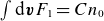 $\int \mathrm{d}{\boldsymbol{v}} F_1 = C n_0$
.
$\int \mathrm{d}{\boldsymbol{v}} F_1 = C n_0$
.
Taking the initial distribution function to be bi-Maxwellian,
 \begin{equation} f_{B} = n \left ( \frac {m}{2 \pi T_\perp ^{2/3}T_\|^{1/3}} \right )^{3/2} \exp \left [ -\frac {\epsilon }{T_{\|}} + \mu B \left ( \frac {1}{T_{\|} } - \frac {1}{T_{\perp }} \right )\right ]\!, \end{equation}
where $T_{\|}$
and
$T_{\|}$
and $T_{\perp }$
measure the parallel and perpendicular temperatures. Setting
$T_{\perp }$
measure the parallel and perpendicular temperatures. Setting $n=n_0(1+\nu )$
,
$n=n_0(1+\nu )$
, $T_\|=T_{\|,0}(1+\tau _\|)$
,
$T_\|=T_{\|,0}(1+\tau _\|)$
, $T_\perp =T_{\perp ,0}(1+\tau _\perp )$
and expanding around the smallness of
$T_\perp =T_{\perp ,0}(1+\tau _\perp )$
and expanding around the smallness of $\nu \sim \tau _\perp \sim \tau _\| \sim \varepsilon$
gives
$\nu \sim \tau _\perp \sim \tau _\| \sim \varepsilon$
gives
 \begin{equation} f_1 = f_{B,0} \left [ \nu + \left ( \frac {\mu B}{T_{\perp ,0}}-1 \right )\tau _{\perp } + \left ( \frac {\epsilon - \mu B}{T_{\|,0}}- \frac {1}{2}\right )\tau _{\|} \right ]\!. \end{equation}
Noting that $\partial _\epsilon f_{B,0} = - f_{B,0}/T_{\|,0}$
, it follows that the ground state is described as
$\partial _\epsilon f_{B,0} = - f_{B,0}/T_{\|,0}$
, it follows that the ground state is described as
 \begin{align} \kappa _1 = T_{\|,0} \left ( C - \tilde {\nu } \right ), \quad F_1 = f_{B,0} \left [ C + \left ( \frac {\mu B}{T_{\perp ,0}}-1 \right )\langle \tau _{\perp } \rangle + \left ( \frac {\epsilon - \mu B}{T_{\|,0}}- \frac {1}{2}\right ) \langle \tau _{\|} \rangle \right ]\!,\nonumber\\[-10pt]\nonumber\\ \end{align}
where we have used $\langle \nu \rangle = \langle \tilde {\nu } \rangle = 0$
. Filling these results into (4.25) gives
$\langle \nu \rangle = \langle \tilde {\nu } \rangle = 0$
. Filling these results into (4.25) gives
 \begin{equation} A = \frac {V n_0 T_{\|,0}}{2} \left \langle \nu ^2 - \tilde {\nu }^2 +\frac {1}{2} \left ( \tau _\|^2 - \langle \tau _\|^2 \rangle \right ) + \tau _\perp ^2 - \langle \tau _\perp ^2 \rangle \right \rangle , \end{equation}
which generalises the result of Helander & Mackenbach (Reference Helander and Mackenbach2024) to $\tilde {\nu } \neq 0$
. Somewhat surprisingly, we see that for a plasma with isotropic temperatures, the result reduces to the case without invariants. Thus, an isotropic plasma that is in its ground state with a given density profile frees up the same amount of available energy to leading order in closeness to a ground state, regardless if a constant magnetic field is present or not. A spatially varying magnetic field and/or the introduction of anisotropy reduces the available energy below its unmagnetised counterpart. However, Poisson’s equation is adjusted when a sufficiently strong magnetic field is present so that a consistent coupling of ground states leads to differing behaviours of it, as we see in the next section.
$\tilde {\nu } \neq 0$
. Somewhat surprisingly, we see that for a plasma with isotropic temperatures, the result reduces to the case without invariants. Thus, an isotropic plasma that is in its ground state with a given density profile frees up the same amount of available energy to leading order in closeness to a ground state, regardless if a constant magnetic field is present or not. A spatially varying magnetic field and/or the introduction of anisotropy reduces the available energy below its unmagnetised counterpart. However, Poisson’s equation is adjusted when a sufficiently strong magnetic field is present so that a consistent coupling of ground states leads to differing behaviours of it, as we see in the next section.
4.5. Ions and electrons in a constant magnetic field
We consider again an ion–electron plasma now in the presence of a constant magnetic field, a so-called slab. To make further progress, we will take finite-Larmor-radius effects to be small, i.e. $ \rho _i k_\perp \ll 1$
, where
$ \rho _i k_\perp \ll 1$
, where $k_\perp$
is the wave vector perpendicular to the magnetic field and
$k_\perp$
is the wave vector perpendicular to the magnetic field and $\rho _i = \sqrt {m_i T_i}/(\mathrm{e} B )$
is the ion Larmor radius (
$\rho _i = \sqrt {m_i T_i}/(\mathrm{e} B )$
is the ion Larmor radius ( $m_i$
being the ion mass). The invariant energy in the electrostatic, long wavelength limit of gyrokinetics is given as (Dubin et al. Reference Dubin, Krommes, Oberman and Lee1983, see also Helander Reference Helander2017, Appendix A)
$m_i$
being the ion mass). The invariant energy in the electrostatic, long wavelength limit of gyrokinetics is given as (Dubin et al. Reference Dubin, Krommes, Oberman and Lee1983, see also Helander Reference Helander2017, Appendix A)
 \begin{align} E_{\mathrm{tot}} \approx & \int \mathrm{d}{\boldsymbol{x}} \epsilon f_i + \int \mathrm{d}{\boldsymbol{x}} \epsilon f_e + \int \mathrm{d}{\boldsymbol{r}} \frac {|\boldsymbol{\nabla }\phi |^2}{8 \pi } + \frac {m_i n_0}{2 B^2} \int \mathrm{d}{\boldsymbol{r}} | \boldsymbol{b} \times \boldsymbol{\nabla }\phi |^2, \end{align}
where the unit magnetic-field vector is given as $\boldsymbol{b} = \boldsymbol{B}/B$
and
$\boldsymbol{b} = \boldsymbol{B}/B$
and $\epsilon = \mu B + mv_\|^2/2$
. Besides the field energy, a kinetic ‘sloshing’ energy (the last term in (4.51)) is now present also, so that the available energy bounds the sum. Furthermore, Poisson’s equation with adiabatic electrons and small
$\epsilon = \mu B + mv_\|^2/2$
. Besides the field energy, a kinetic ‘sloshing’ energy (the last term in (4.51)) is now present also, so that the available energy bounds the sum. Furthermore, Poisson’s equation with adiabatic electrons and small $\rho _i k_\perp$
becomes
$\rho _i k_\perp$
becomes
 \begin{align} \tilde {\nu }_{i,\boldsymbol{k}} &\approx \left ( \frac {T_i}{T_e} + \rho _i^2 k_\perp ^2 + \lambda _{D,i}^2 k^2 \right ) \hat {\phi }_{\boldsymbol{k}} \nonumber\\ &\approx \varPhi _i(\boldsymbol{k}) \hat {\phi }_{\boldsymbol{k}}, \end{align}
where $\tilde {\nu }_{i,\boldsymbol{k}}$
denotes the
$\tilde {\nu }_{i,\boldsymbol{k}}$
denotes the $\boldsymbol{k}$
th Fourier component of density fluctuations associated with the ground state of
$\boldsymbol{k}$
th Fourier component of density fluctuations associated with the ground state of $f_i$
, the electrostatic potential is normalised as
$f_i$
, the electrostatic potential is normalised as $\hat {\phi }_{\boldsymbol{k}} = \mathrm{e} \phi _{\boldsymbol{k}} / T_i$
and the shorthand
$\hat {\phi }_{\boldsymbol{k}} = \mathrm{e} \phi _{\boldsymbol{k}} / T_i$
and the shorthand $\varPhi (\boldsymbol{k})$
is used for the factor in brackets.Footnote
9
Assume that the initial distribution
$\varPhi (\boldsymbol{k})$
is used for the factor in brackets.Footnote
9
Assume that the initial distribution $f_i$
is given as a Maxwellian (as is
$f_i$
is given as a Maxwellian (as is $f_e$
) with slight variations in temperature and density, so that the sum of the two available energies gives the total
$f_e$
) with slight variations in temperature and density, so that the sum of the two available energies gives the total
 \begin{equation} A = A_{\mathrm{G}} - \frac {n_0 T_i (2\pi )^3}{2} \int \mathrm{d}{\boldsymbol{k}}\, | \varPhi _i(\boldsymbol{k})\hat {\phi }_{\boldsymbol{k}} |^2 - \frac {n_0 T_i (2\pi )^3}{2} \int \mathrm{d}{\boldsymbol{k}}\, \frac {T_i}{T_e} |\hat {\phi }_{\boldsymbol{k}}|^2. \end{equation}
In order to satisfy the conservation of (4.51), one must have
 \begin{equation} A_{\mathrm{G}} = \frac {n_0 T_i (2 \pi )^3}{2} \int \mathrm{d}{\boldsymbol{k}}\, | \hat {\phi }_{\boldsymbol{k}} |^2 \left ( |\varPhi _i(\boldsymbol{k})|^2 + \frac {T_i}{T_e} +\rho _i^2 k_\perp ^2 + \lambda _{D,i}^2 k^2 \right )\!, \end{equation}
which – as in (3.15) and (3.16) – may be achieved by defining the distribution
 \begin{equation} \varphi (\boldsymbol{k}) = \frac {n_0 T_i (2\pi )^3}{2A_{\mathrm{G}}} | \hat {\phi }_{\boldsymbol{k}} |^2 \left ( |\varPhi _i(\boldsymbol{k})|^2 + \frac {T_i}{T_e} + \rho _i^2 k_\perp ^2 + \lambda _{D,i}^2 k^2 \right )\!, \end{equation}
whose integral over wavenumber space satisfies $\int \mathrm{d}{\boldsymbol{k}} \varphi ({\boldsymbol{k}}) = 1$
. The available energy then becomes
$\int \mathrm{d}{\boldsymbol{k}} \varphi ({\boldsymbol{k}}) = 1$
. The available energy then becomes
 \begin{equation} \frac {A}{A_{\mathrm{G}}} = \int \mathrm{d}{\boldsymbol{k}}\, \varphi (\boldsymbol{k}) \frac { \rho _i^2 k_\perp ^2 + \lambda _{D,i}^2 k^2 }{ |\varPhi _i(\boldsymbol{k})|^2 + ({T_i}/{T_e}) + \rho _i^2 k_\perp ^2 + \lambda _{D,i}^2 k^2} \leqslant 1 , \end{equation}
which again may be maximised by finding the wave vector $\boldsymbol{k}=\boldsymbol{k}_0$
that does so. Setting the magnitude of the wavenumber
$\boldsymbol{k}=\boldsymbol{k}_0$
that does so. Setting the magnitude of the wavenumber $k^2 = k_\perp ^2 + k_z^2$
where the perpendicular component is
$k^2 = k_\perp ^2 + k_z^2$
where the perpendicular component is $k_\perp ^2 = k_x^2 + k_y^2$
(i.e. the metric tensor is diagonal and constant) yields a maximising perpendicular wavenumber
$k_\perp ^2 = k_x^2 + k_y^2$
(i.e. the metric tensor is diagonal and constant) yields a maximising perpendicular wavenumber
 \begin{equation} \big(\rho _i^2 + \lambda _{D,i}^2\big)k_\perp ^2 =-\lambda _{D,i}^2 k_z^2 + \sqrt {\frac {T_i^2}{T_e^2} + \frac {T_i}{T_e}}, \end{equation}
where solubility requires that $\lambda _{D,i}^2k_z^2 \leqslant \sqrt {({T_i^2}/{T_e^2}) + ({T_i}/{T_e})}$
. Note the close correspondence to the result given in (4.39), as setting
$\lambda _{D,i}^2k_z^2 \leqslant \sqrt {({T_i^2}/{T_e^2}) + ({T_i}/{T_e})}$
. Note the close correspondence to the result given in (4.39), as setting $\rho _i = 0$
gives the same maximising wavenumber magnitude. Indeed, the available energy is unchanged and becomes
$\rho _i = 0$
gives the same maximising wavenumber magnitude. Indeed, the available energy is unchanged and becomes
 \begin{equation} A = \left ( 1 - \frac {4}{2 + 2 \sqrt {1 + T_e/T_i}} \right ) A_{\mathrm{G}}, \end{equation}
the exact same result as in (4.38). This is perhaps unsurprising, as one can still deposit the energy in electrostatic modes in this regime, though it is no longer solely in the form of the field energy. The energy is distributed between the field and sloshing terms as
 \begin{equation} \frac {\int \mathrm{d}{\boldsymbol{r}}\, |\boldsymbol{\nabla }\phi |^2/8\pi }{\int \mathrm{d}{\boldsymbol{r}}\, m_i n_0 |\boldsymbol{b} \times \boldsymbol{\nabla }\phi |/2B^2} = \frac {\lambda _{D,i}^2}{\rho _i^2} \left (\frac { \sqrt {({T_i^2}/{T_e^2}) + ({T_i}/{T_e})} + \rho _i^2 k_z^2}{\sqrt { ({T_i^2}/{T_e^2}) + ({T_i}/{T_e}}) - \lambda _{D,i}^2 k_z^2} \right )\!. \end{equation}
Since strongly magnetised plasmas tend to be very anisotropic, $\rho _i k_z \sim \rho _i/L \ll 1$
and
$\rho _i k_z \sim \rho _i/L \ll 1$
and $\lambda _{D,i} k_z \sim \lambda _{D,i}/L \ll 1$
, where
$\lambda _{D,i} k_z \sim \lambda _{D,i}/L \ll 1$
, where $L$
is some global length scale (in a magnetic confinement device
$L$
is some global length scale (in a magnetic confinement device $L$
is of the order of the major radius), the ratio of the field-to-sloshing energy is approximately
$L$
is of the order of the major radius), the ratio of the field-to-sloshing energy is approximately $\lambda _{D,i}^2/\rho _i^2$
. In most practical applications
$\lambda _{D,i}^2/\rho _i^2$
. In most practical applications $\lambda _{D,i} \ll \rho _i$
, meaning that one can safely neglect
$\lambda _{D,i} \ll \rho _i$
, meaning that one can safely neglect $\lambda _{D,i}$
effects in the ground state.
$\lambda _{D,i}$
effects in the ground state.
Increasing $T_e/T_i$
in its large-value limit we see two behaviours of interest: firstly, for
$T_e/T_i$
in its large-value limit we see two behaviours of interest: firstly, for $\lambda _{D,i}= 0$
, the maximising wavenumber (4.57) goes as
$\lambda _{D,i}= 0$
, the maximising wavenumber (4.57) goes as $\rho _i^2 k_\perp ^2 \approx \sqrt {T_i/T_e}$
, confirming that the long-wavelength assumption is satisfied here, and one could furthermore expect that the transport is greatly enhanced by being concentrated in long wavelengths. A similar behaviour is present in the simple Vlasov–Poisson plasma, as for fixed ion-temperature and large
$\rho _i^2 k_\perp ^2 \approx \sqrt {T_i/T_e}$
, confirming that the long-wavelength assumption is satisfied here, and one could furthermore expect that the transport is greatly enhanced by being concentrated in long wavelengths. A similar behaviour is present in the simple Vlasov–Poisson plasma, as for fixed ion-temperature and large $T_e/T_i$
, (4.39) goes as
$T_e/T_i$
, (4.39) goes as $\lambda _{D,i}^2k^2 \approx \sqrt {T_i/T_e}$
. Secondly, the transport could be exacerbated further when increasing
$\lambda _{D,i}^2k^2 \approx \sqrt {T_i/T_e}$
. Secondly, the transport could be exacerbated further when increasing $T_e/T_i$
as the available energy (4.58) goes as
$T_e/T_i$
as the available energy (4.58) goes as $A \approx A_{\mathrm{G}}(1 - 2\sqrt {T_i/T_e})$
, approaching the Gardner bound as the electron temperature is raised at fixed ion temperature. The amplification of transport with increasing
$A \approx A_{\mathrm{G}}(1 - 2\sqrt {T_i/T_e})$
, approaching the Gardner bound as the electron temperature is raised at fixed ion temperature. The amplification of transport with increasing $T_e$
at fixed
$T_e$
at fixed $T_i$
is a known feature of gyrokinetic turbulence having been found both in dispersion relations and simulations (Biglari, Diamond & Rosenbluth Reference Biglari, Diamond and Rosenbluth1989; Romanelli Reference Romanelli1989; Plunk et al. Reference Plunk, Helander, Xanthopoulos and Connor2014; Zocco et al. Reference Zocco, Xanthopoulos, Doerk, Connor and Helander2018; Helander & Plunk Reference Helander and Plunk2022), and may be a possible culprit degrading energy confinement in both tokamaks and stellarators that are electron heated (Beurskens et al. Reference Beurskens2021). In the simple model considered, we may understand it simply as the upper bound on the combined field and kinetic energy growing, which can lead to increased transport if the system approaches the bound (in value or in scaling), where an increase in the maximising wavelength furthermore contributes.
$T_i$
is a known feature of gyrokinetic turbulence having been found both in dispersion relations and simulations (Biglari, Diamond & Rosenbluth Reference Biglari, Diamond and Rosenbluth1989; Romanelli Reference Romanelli1989; Plunk et al. Reference Plunk, Helander, Xanthopoulos and Connor2014; Zocco et al. Reference Zocco, Xanthopoulos, Doerk, Connor and Helander2018; Helander & Plunk Reference Helander and Plunk2022), and may be a possible culprit degrading energy confinement in both tokamaks and stellarators that are electron heated (Beurskens et al. Reference Beurskens2021). In the simple model considered, we may understand it simply as the upper bound on the combined field and kinetic energy growing, which can lead to increased transport if the system approaches the bound (in value or in scaling), where an increase in the maximising wavelength furthermore contributes.
4.5.1. Zonal flows
The fact that the ground state derived in the preceding section allows for radial streamers (that is, $k_x=0$
modes) is reminiscent of results found by Hammett et al. (Reference Hammett, Beer, Dorland, Cowley and Smith1993), who simulated ion-temperature-gradient-driven turbulence using a nonlinear gyrofluid model assuming that
$k_x=0$
modes) is reminiscent of results found by Hammett et al. (Reference Hammett, Beer, Dorland, Cowley and Smith1993), who simulated ion-temperature-gradient-driven turbulence using a nonlinear gyrofluid model assuming that $\delta n_e \propto \phi$
, and found that the turbulent state does not saturate due to these streamers. Saturation is achieved by correcting the adiabatic response,
$\delta n_e \propto \phi$
, and found that the turbulent state does not saturate due to these streamers. Saturation is achieved by correcting the adiabatic response,
 \begin{equation} \frac {\delta n_e}{n_0} = \frac {\mathrm{e} (\phi - \langle \phi \rangle _{\mathrm{fs}})}{T_e}, \end{equation}
where the flux-surface average of the electrostatic potential, denoted as $\langle \phi \rangle _{\mathrm{fs}}$
, is subtracted due to the rapid circulation of electrons around the flux surface. It is worthwhile to compare this behaviour to the results found in § 3: for purely zonal potentials (
$\langle \phi \rangle _{\mathrm{fs}}$
, is subtracted due to the rapid circulation of electrons around the flux surface. It is worthwhile to compare this behaviour to the results found in § 3: for purely zonal potentials ( $\phi = \langle \phi \rangle _{\mathrm{fs}}$
), the background density is unperturbed and acts like the neutralising case of the waterbags. In the language of zonal-flow literature, this is because such flows are modes of minimal inertia (Diamond et al. Reference Diamond, Itoh, Itoh and Hahm2005): they are not screened by the Boltzmann response of the electrons. Focusing on the ground state, by concentrating the energy into arbitrarily long wavelength zonal flows we thus expect that the Gardner bound can be reached, which is indeed what we find.
$\phi = \langle \phi \rangle _{\mathrm{fs}}$
), the background density is unperturbed and acts like the neutralising case of the waterbags. In the language of zonal-flow literature, this is because such flows are modes of minimal inertia (Diamond et al. Reference Diamond, Itoh, Itoh and Hahm2005): they are not screened by the Boltzmann response of the electrons. Focusing on the ground state, by concentrating the energy into arbitrarily long wavelength zonal flows we thus expect that the Gardner bound can be reached, which is indeed what we find.
The flux-surface average in Fourier space is equivalent to setting $\hat {\phi }_{\mathrm{Z}} = \hat {\phi }_{\boldsymbol{k}}(k_x,$ $k_y=0,k_z=0)$
(where the subscript
$k_y=0,k_z=0)$
(where the subscript $\mathrm{Z}$
stands for the zonal component), thus retaining radial dependence alone. Similarly, using this response in our calculation modifies Poisson’s equation to
$\mathrm{Z}$
stands for the zonal component), thus retaining radial dependence alone. Similarly, using this response in our calculation modifies Poisson’s equation to
 \begin{equation} \tilde {\nu }_{i,\boldsymbol{k}} \approx \begin{cases} \left (\varPhi _i(\boldsymbol{k}) - \dfrac {T_i}{T_e} \right )\hat {\phi }_{\mathrm{Z}} & \text{if } k_y=k_z=0, \\[3pt] \varPhi _i(\boldsymbol{k}) \hat {\phi }_{\boldsymbol{k}} & \text{otherwise}. \end{cases} \end{equation}
Supposing that the potential is purely zonal ( $k_y=k_z=0$
, consequently
$k_y=k_z=0$
, consequently $\hat {\phi }_{\boldsymbol{k}}=\hat {\phi }_{\mathrm{Z}}$
), we may proceed with the calculation as before, with the total available energy (4.53) being adjusted to
$\hat {\phi }_{\boldsymbol{k}}=\hat {\phi }_{\mathrm{Z}}$
), we may proceed with the calculation as before, with the total available energy (4.53) being adjusted to
 \begin{equation} A = A_{\mathrm{G}} - \frac {n_0 T_i (2\pi )}{2} \int \mathrm{d}{k_x} \left ( \varPhi _i(k_x) -\frac {T_i}{T_e} \right )^2 |\hat {\phi }_{\mathrm{Z}} |^2, \end{equation}
whereas conservation of energy (4.54) now gives
 \begin{equation} A_{\mathrm{G}} = \frac {n_0 T_i (2 \pi )}{2} \int \mathrm{d}{k_x} \left [ \left (\varPhi _i(k_x) - \frac {T_i}{T_e} \right )^2 +\rho _i^2 k_x^2 + \lambda _{D,i}^2 k_x^2 \right ] | \hat {\phi }_{\mathrm{Z}} |^2. \end{equation}
As before, we define the distribution $\varphi (k_x)$
,
$\varphi (k_x)$
,
 \begin{equation} \varphi (k_x) = \frac {n_0 T_i (2\pi )}{2A_{\mathrm{G}}} \left [ \left (\varPhi _i(k_x) - \frac {T_i}{T_e} \right )^2 +\rho _i^2 k_x^2 + \lambda _{D,i}^2 k_x^2 \right ]| \hat {\phi }_{\mathrm{Z}} |^2, \end{equation}
so that the part of the Gardner bound that may be released becomes
 \begin{equation} \frac {A}{A_{\mathrm{G}}} = \int \mathrm{d}{k_x} \frac { \varphi (k_x)}{ 1 + \big(\rho _i^2 + \lambda _{D,i}^2\big) k_x^2 } \leqslant 1. \end{equation}
For a Dirac-delta $\varphi$
at
$\varphi$
at $k_x = k_{x,0}$
, we thus find that
$k_x = k_{x,0}$
, we thus find that
 \begin{equation} \frac {A}{A_{\mathrm{G}}} = \frac {1}{1+\big(\rho _i^2+\lambda _{D,i}^2\big)k_{x,0}^2} \end{equation}
is completely analogously to the waterbag calculation with a neutralising background, where the Gardner bound is reached for $k_{x,0}\rightarrow 0$
. This gives an interesting example of a state that has no transport due to the stabilising zonal structure, despite having reached the Gardner bound. Furthermore, the ground state is a zonally dominated state, as is the case in the Dimits regime (Dimits et al. Reference Dimits2000).
$k_{x,0}\rightarrow 0$
. This gives an interesting example of a state that has no transport due to the stabilising zonal structure, despite having reached the Gardner bound. Furthermore, the ground state is a zonally dominated state, as is the case in the Dimits regime (Dimits et al. Reference Dimits2000).
4.6. Impurities subject to quasineutrality
We consider a crude model to capture the available energy of three different Maxwellian species of particles in a toroidal geometry, namely electrons (trapped and passing), hydrogen and an additional impurity species with charge number $Z$
. We model the trapped electrons and both ion species as having no invariants aside from the Casimirs, whereas the passing electron species due to its fast motion along the field line (averaging the radial drift to zero) conserves its flux-surface label
$Z$
. We model the trapped electrons and both ion species as having no invariants aside from the Casimirs, whereas the passing electron species due to its fast motion along the field line (averaging the radial drift to zero) conserves its flux-surface label $\psi$
. This is, of course, a gross oversimplification. In reality, all species obey conservation of
$\psi$
. This is, of course, a gross oversimplification. In reality, all species obey conservation of $\mu$
, and the trapped electron species furthermore conserves the parallel invariant as treated in Mackenbach et al. (Reference Mackenbach, Proll, Wakelkamp and Helander2023). However, we are not too interested in capturing the Gardner value of the available energy accurately here, and we instead wish to focus on how the constraint of quasineutrality reduces this Gardner bound, continuing as such.
$\mu$
, and the trapped electron species furthermore conserves the parallel invariant as treated in Mackenbach et al. (Reference Mackenbach, Proll, Wakelkamp and Helander2023). However, we are not too interested in capturing the Gardner value of the available energy accurately here, and we instead wish to focus on how the constraint of quasineutrality reduces this Gardner bound, continuing as such.
In a toroidal geometry the density and temperature are flux functions, $\nu _{e,p} = \nu _{e,p}(\psi )$
and
$\nu _{e,p} = \nu _{e,p}(\psi )$
and $\tau _{e,p} = \tau _{e,p}(\psi )$
, rendering it impossible for the passing electron species to liberate available energy (as the plasma distribution function is a ground state at fixed
$\tau _{e,p} = \tau _{e,p}(\psi )$
, rendering it impossible for the passing electron species to liberate available energy (as the plasma distribution function is a ground state at fixed $\psi$
, consequently keeping the density and temperature profiles of these particles fixed). In order to have quasineutrality, one thus requires that
$\psi$
, consequently keeping the density and temperature profiles of these particles fixed). In order to have quasineutrality, one thus requires that
 \begin{equation} f_p\nu _{e,p}(\psi ) + (1-f_p) \tilde {\nu }_{e,t}(\psi ) = \frac {n_H}{n_e}\tilde {\nu }_{H}(\psi ) + \frac {Zn_Z}{n_e} \tilde {\nu }_{Z}(\psi ), \end{equation}
where the subscripts $e$
,
$e$
, $H$
and
$H$
and $Z$
denote whether we are dealing with electrons, hydrogen or the remaining ionic species, respectively. Furthermore, subscripts
$Z$
denote whether we are dealing with electrons, hydrogen or the remaining ionic species, respectively. Furthermore, subscripts $t$
and
$t$
and $p$
indicates if the electrons are trapped or passing and
$p$
indicates if the electrons are trapped or passing and $f_p \in [0,1]$
denotes the passing fraction (related to the trapping fraction
$f_p \in [0,1]$
denotes the passing fraction (related to the trapping fraction $f_t$
as
$f_t$
as $f_t = 1-f_p$
). The available energy, assuming initially Maxwellian distribution functions with slightly varying density and temperature, becomes
$f_t = 1-f_p$
). The available energy, assuming initially Maxwellian distribution functions with slightly varying density and temperature, becomes
 \begin{equation} A = A_{\mathrm{G} } - \frac {n_e T_{e} V (1-f_p)^2}{2} \langle \tilde {\nu }_{e,t}^2 \rangle - \frac {n_H T_{H} V}{2} \langle \tilde {\nu }_{H}^2 \rangle - \frac {n_Z T_{Z} V}{2} \langle \tilde {\nu }_{Z}^2 \rangle . \end{equation}
It is evident that in order to maximise (4.68) the trapped electron density variation can be set to zero, leaving only the ion densities to optimise over. Solving (4.67) for $\tilde {\nu }_Z$
and substituting this expression into (4.68) gives
$\tilde {\nu }_Z$
and substituting this expression into (4.68) gives
 \begin{equation} A = A_{\mathrm{G} } - \frac {n_e T_{H} V}{2} \langle \tilde {\nu }_{H}^2 \rangle - \frac {n_Z T_{Z} V}{2Z^2} \left \langle \left ( \frac { n_e f_p \nu _{e,p}}{n_Z} - \frac {n_H \tilde {\nu }_{H}}{n_Z} \right )^2 \right \rangle , \end{equation}
which is maximal for
 \begin{equation} \tilde {\nu }_{H}(\psi ) = \frac {f_p n_0 T_{Z}}{n_HT_{Z} + Z^2 n_Z T_{H}} \nu _{e,p}(\psi ). \end{equation}
Using this equation for the available energy and using the zeroth-order solution of the quasineutrality condition $n_e = n_H + Zn_Z$
, we obtain the result
$n_e = n_H + Zn_Z$
, we obtain the result
 \begin{equation} A = A_{\mathrm{G}} - \frac {f_p^2 n_e^2 T_H T_Z V}{2( n_H T_Z + Z^2n_Z T_H ) } \langle \nu _{e,p}^2 \rangle . \end{equation}
It is clear that having a high charge-number species present in the plasma (at fixed number densities) is disadvantageous not only in terms of having higher radiation losses or rarefying the fusion fuel, it also increases the available energy and may thus enhance turbulence in this very crude model. The reason for this is simple: if the charge number is very high, one can satisfy (4.67) with small values of $\tilde {\nu }_H$
and
$\tilde {\nu }_H$
and $\tilde {\nu }_Z$
, requiring little density variation in the ground state and thus approaching the Gardner value. However, this argument ignores the fact that the Gardner bound itself may depend on
$\tilde {\nu }_Z$
, requiring little density variation in the ground state and thus approaching the Gardner value. However, this argument ignores the fact that the Gardner bound itself may depend on $Z$
and other parameters, and we wish to analyse such dependencies in the following paragraph.
$Z$
and other parameters, and we wish to analyse such dependencies in the following paragraph.
To investigate dependence on impurity content $n_Z$
, let us assume that the initial states all have variation in density alone, further assuming that
$n_Z$
, let us assume that the initial states all have variation in density alone, further assuming that $\nu _{e,t}=\nu _{e,p}=\nu _e$
, so that the Gardner bound becomes
$\nu _{e,t}=\nu _{e,p}=\nu _e$
, so that the Gardner bound becomes
 \begin{equation} A_{\mathrm{G}} = \frac {n_H T_H V}{2} \langle \nu _{H}^2 \rangle + \frac {n_e T_e f_p V}{2} \langle \nu _{e}^2 \rangle + \frac {n_Z T_Z V}{2} \langle \nu _{Z}^2 \rangle . \end{equation}
The initial states also have to be quasineutral ( $n_e=n_H+Zn_Z$
), meaning that
$n_e=n_H+Zn_Z$
), meaning that
 \begin{equation} \nu _{e}(\psi ) = \frac {n_H}{n_0}\nu _{H}(\psi ) + \frac {Zn_Z}{n_0} \nu _{Z}(\psi ). \end{equation}
The precise functional form of $A(n_Z)$
depends, of course, on what is held constant as
$A(n_Z)$
depends, of course, on what is held constant as $n_Z$
is varied, and we make the following choices: we use the quasineutrality equations to eliminate dependence on
$n_Z$
is varied, and we make the following choices: we use the quasineutrality equations to eliminate dependence on $n_e$
and
$n_e$
and $\nu _e$
, set
$\nu _e$
, set $T_H=T_Z=T_e=T$
and express the impurity density in terms of the effective charge
$T_H=T_Z=T_e=T$
and express the impurity density in terms of the effective charge $Z_{\mathrm{eff}} = n_H/n_e + Z^2 n_Z/n_e$
, and define a relative available energy
$Z_{\mathrm{eff}} = n_H/n_e + Z^2 n_Z/n_e$
, and define a relative available energy $\overline {A}=A/A(Z_{\mathrm{eff}}=0)$
. Further specialising to the case where
$\overline {A}=A/A(Z_{\mathrm{eff}}=0)$
. Further specialising to the case where $\langle \nu _H^2 \rangle = 1$
,
$\langle \nu _H^2 \rangle = 1$
, $\langle \nu _H \nu _Z \rangle = 1/4$
,
$\langle \nu _H \nu _Z \rangle = 1/4$
, $\langle \nu _Z^2 \rangle = 1/16$
,
$\langle \nu _Z^2 \rangle = 1/16$
, $f_p=1/3$
and
$f_p=1/3$
and $Z=6$
gives a relative available energy dependent on only
$Z=6$
gives a relative available energy dependent on only $Z_{\mathrm{eff}}$
(which itself depends on
$Z_{\mathrm{eff}}$
(which itself depends on $n_H$
), namely
$n_H$
), namely
 \begin{equation} \overline {A} = \frac {-486 Z_{\mathrm{eff}}-({1350}/{Z_{\mathrm{eff}}-6})-({529}/{Z_{\mathrm{eff}}})+5065}{4320}. \end{equation}
A plot of this function is given in figure 8, where we see a pronounced minimum in $\overline {A}$
for a certain
$\overline {A}$
for a certain $Z_{\mathrm{eff}}$
. Similar dependence was found in García-Regaña et al. (Reference García-Regaña, Calvo, Parra and Thienpondt2024) for the turbulent transport, though we stress that the parameters chosen here are not the same – we are more interested in seeing if qualitative behaviours are captured, since the model we have used is crude. The fact that qualitatively such trends arise may indicate that the intricate dependencies of turbulent transport on impurities can be, in part, captured by considerations of energy budgets in conjunction with quasineutrality.
$Z_{\mathrm{eff}}$
. Similar dependence was found in García-Regaña et al. (Reference García-Regaña, Calvo, Parra and Thienpondt2024) for the turbulent transport, though we stress that the parameters chosen here are not the same – we are more interested in seeing if qualitative behaviours are captured, since the model we have used is crude. The fact that qualitatively such trends arise may indicate that the intricate dependencies of turbulent transport on impurities can be, in part, captured by considerations of energy budgets in conjunction with quasineutrality.
Plot of the relative available energy’s dependence on $Z_{\mathrm{eff}}$
.
$Z_{\mathrm{eff}}$
.

4.7. A kappa distribution in free space
Let us now consider a non-Maxwellian distribution function that is nonetheless a ground state, namely the kappa distribution given as
 \begin{equation} f_\chi (\boldsymbol{x}) = n_0 \left ( \frac {m }{2 \pi T} \right )^{d/2} \frac {\varGamma ( \chi + 1 + {d}/{2} )}{ \chi ^{d/2}\varGamma ( \chi + 1)} \left ( 1 + \frac {1}{\chi } \frac {\epsilon }{T} \right )^{-\chi - 1 - d/2}, \end{equation}
where $d$
denotes the dimensionality (having replaced the typical
$d$
denotes the dimensionality (having replaced the typical $\kappa$
parameter with
$\kappa$
parameter with $\chi$
, since the former is used as a Lagrange multiplier). Perturbing the density and temperature slightly,
$\chi$
, since the former is used as a Lagrange multiplier). Perturbing the density and temperature slightly, $n = n_0(1+\nu )$
and
$n = n_0(1+\nu )$
and $T = T_0 (1 + \tau )$
, gives the leading-order derivative
$T = T_0 (1 + \tau )$
, gives the leading-order derivative
 \begin{equation} f_{\chi ,0}^{\prime} [\epsilon ] = - f_{\chi ,0}[\epsilon ] \frac {1 + \chi + {d}/{2}}{\epsilon +T_0 \chi }, \end{equation}
which is indeed negative definite for any $\chi \gt 0$
, implying it is a ground state. Going to the next order gives the perturbed distribution function
$\chi \gt 0$
, implying it is a ground state. Going to the next order gives the perturbed distribution function
 \begin{equation} f_1(\boldsymbol{x}) = f_{\chi ,0} \left [ \nu + \tau \frac {{\epsilon }/{T_0}(1+\chi ) - {\chi d}/{2}}{{\epsilon }/{T_0} + \chi } \right ]\!. \end{equation}
As in § 4.1, using $\langle \tilde {\nu } \rangle =\langle \nu \rangle =\langle \tau \rangle = 0$
simplifies the ground-state equation (4.18) to
$\langle \tilde {\nu } \rangle =\langle \nu \rangle =\langle \tau \rangle = 0$
simplifies the ground-state equation (4.18) to
 \begin{equation} F_1[\epsilon ] = \frac { C \chi (1 + \chi + {d}/{2} )}{(1+\chi ) ( ({mv^2}/{2T_0}) + \chi )} f_{\chi ,0}, \end{equation}
having defined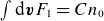 $\int \mathrm{d}{\boldsymbol{v}} F_1 =C n_0$
and having used
$\int \mathrm{d}{\boldsymbol{v}} F_1 =C n_0$
and having used $\int \mathrm{d}{\boldsymbol{v}} F_0^{\prime} = -n_0(1+\chi )/T_0\chi$
. The available energy simplifies to
$\int \mathrm{d}{\boldsymbol{v}} F_0^{\prime} = -n_0(1+\chi )/T_0\chi$
. The available energy simplifies to
 \begin{equation} A = \frac {n_0 T_0 V}{2} \left \langle \frac {d(\nu + \tau )^2 + \chi (2 \nu ^2 + d \tau ^2)}{2+d+2 \chi } \right \rangle - \frac {n_0 T_0 V}{2} \left \langle \frac {\chi \tilde {\nu }^2}{1 + \chi } \right \rangle\! . \end{equation}
The first term is the Gardner bound as derived in Helander & Mackenbach (Reference Helander and Mackenbach2024), whereas the second term encodes the penalty of the ground-state density fluctuation. As shown in Appendix E, even if the density profile is fixed and there are no temperature fluctuations ( $\tilde {\nu } = \nu$
and
$\tilde {\nu } = \nu$
and $\tau =0$
) there is a non-zero available energy, i.e.
$\tau =0$
) there is a non-zero available energy, i.e.
 \begin{equation} A = \frac {n_0 T_0 V}{2} \left \langle \frac {d\nu ^2 }{2(1+\chi )(2+d+2\chi )} \right \rangle , \end{equation}
meaning that energy can be extracted from density fluctuations even if it cannot flatten, indicating that there are phase-space rearrangements possible that release energy. (One such rearrangement for a simplified scenario is shown in figure 14 of Appendix E).
This may have implications for the stability properties of plasmas with non-Maxwellian features, adiabatic electrons and a pure density gradient. In Helander (Reference Helander2020) it is proven that an isothermal Maxwellian with a fixed density profile is nonlinearly stable due to its vanishing available energy. However, as we see here, for any other distribution function, there are phase-space rearrangements possible that liberate energy, meaning some instability can arise.
4.8. A three-dimensional slowing-down distribution in a constant magnetic field
Consider now a distribution function used often to model the fast alpha particles born from fusion reactions, the so-called slowing-down distribution. This distribution function is derived by imposing a Dirac-delta source of particles at a single velocity and solving the steady-state Fokker–Planck equation where the fast particles collide with a Maxwellian background species of electrons (Gaffey Jr Reference Gaffey1976; Moseev & Salewski Reference Moseev and Salewski2019), yielding
 \begin{equation} f_s(\boldsymbol{x}) = \frac {3n}{4 \pi \ln \big( 1 + {v_\alpha ^3}/{v_c^3} \big)} \frac {\varTheta ( v_\alpha - v )}{v^3 + v_c^3}. \end{equation}
Here $n(\boldsymbol{x})$
is the fast-particle density,
$n(\boldsymbol{x})$
is the fast-particle density, $v_c(\boldsymbol{x})$
is the ‘cross-over’ velocity where the drag on fast ions and electrons is equal and
$v_c(\boldsymbol{x})$
is the ‘cross-over’ velocity where the drag on fast ions and electrons is equal and $v_\alpha$
is the velocity of the born alpha particles (so that
$v_\alpha$
is the velocity of the born alpha particles (so that $m_\alpha v_\alpha ^2/2 \approx 3.5 \; \text{MeV}$
). Note that
$m_\alpha v_\alpha ^2/2 \approx 3.5 \; \text{MeV}$
). Note that $\partial _\epsilon f_s \leqslant 0$
, so that a spatially homogeneous slowing-down distribution is a ground state. We wish to find the corresponding ground state of the spatially varying slowing-down distribution function (though the turbulence itself may alter the distribution function Wilkie (Reference Wilkie2018) – an effect that we will ignore). A comment is warranted here, as the available energy tells us how much energy can be released collisionlessly, whereas the slowing-down distribution is created by a collisional process. As such, one can best interpret the results as a measure of how unstable such a collisional distribution is to collisionless instabilities. A proper analysis should take into account the ordering of the different time scales (slowing-down time, growth rate of collisionless instabilities, etc.), we shall not attempt to do so here.
$\partial _\epsilon f_s \leqslant 0$
, so that a spatially homogeneous slowing-down distribution is a ground state. We wish to find the corresponding ground state of the spatially varying slowing-down distribution function (though the turbulence itself may alter the distribution function Wilkie (Reference Wilkie2018) – an effect that we will ignore). A comment is warranted here, as the available energy tells us how much energy can be released collisionlessly, whereas the slowing-down distribution is created by a collisional process. As such, one can best interpret the results as a measure of how unstable such a collisional distribution is to collisionless instabilities. A proper analysis should take into account the ordering of the different time scales (slowing-down time, growth rate of collisionless instabilities, etc.), we shall not attempt to do so here.
Set $n = n_0( 1 + \nu )$
and
$n = n_0( 1 + \nu )$
and $v_c = v_{c,0}(1 + \tau /2)$
since
$v_c = v_{c,0}(1 + \tau /2)$
since $v_c \propto \sqrt {T_e}$
, though
$v_c \propto \sqrt {T_e}$
, though $\tau$
may include spatial variation in the main ion and electron densities too (see Wilkie Reference Wilkie2015, Equation (1.22)). The perturbed distribution function is
$\tau$
may include spatial variation in the main ion and electron densities too (see Wilkie Reference Wilkie2015, Equation (1.22)). The perturbed distribution function is
 \begin{equation} f_{s,1} = f_{s,0} \left \{ \nu + \frac {3 \tau }{2} \left [ \frac {v_\alpha ^3}{\big(v_\alpha ^3 + v_{c,0}^3\big) \ln \big( 1 + {v_\alpha ^3}/{v_{c,0}^3} \big)} - \frac {v_{c,0}^3}{v_{c,0}^3 + v^3} \right ] \right \}\!. \end{equation}
The ground state in a constant magnetic field is given by (4.45), (4.46), and for these equations, we require $\partial _\epsilon f_{s,0}$
and its integral over velocity space. These may be evaluated analytically as
$\partial _\epsilon f_{s,0}$
and its integral over velocity space. These may be evaluated analytically as
 \begin{equation} \partial _\epsilon f_{s,0} = -\frac {9 n_0}{4 \pi m \ln \big( 1 + {v_\alpha ^3}/{v_{c,0}^3} \big)} \left \{\frac {v \varTheta [v_\alpha - v]}{\big( v_{c,0}^3 + v^3 \big)^2} + \frac {\delta [v_\alpha - v]}{3v\big( v_{c,0}^3 + v^3 \big)} \right \} \end{equation}
and
 \begin{align} \int \mathrm{d}{\boldsymbol{v}} \partial _\epsilon f_{s,0} = -&\frac {n_0}{2 m v_{c,0}^2 \ln \big( 1 + {v_\alpha ^3}/{v_{c,0}^3} \big)} \times \Bigg ( \frac {\pi }{\sqrt {3}} - 2\sqrt {3} \cot ^{-1} \left [ \frac {v_{c,0} \sqrt {3}}{v_{c,0} - 2 v_{\alpha }} \right ] \nonumber\\ & +2 \ln [ v_{c,0} + v_{\alpha } ] - \ln \big[ v_{c,0}^2 + v_\alpha ^2 - v_{c,0} v_\alpha \big] \Bigg ) \nonumber\\ \equiv & -\frac {n_0}{2m v_{c,0}^2 \ln \big( 1 +{v_\alpha ^3}/{v_{c,0}^3} \big)} \times \mathcal{E}(v_{c,0},v_\alpha ), \end{align}
where $\cot ^{-1}(x)$
is the inverse of
$\cot ^{-1}(x)$
is the inverse of $\cot (x)=1/\tan (x)$
, and having defined the factor in brackets as
$\cot (x)=1/\tan (x)$
, and having defined the factor in brackets as $\mathcal{E}(v_{c,0},v_\alpha )$
. As such, the Lagrange multiplier satisfies
$\mathcal{E}(v_{c,0},v_\alpha )$
. As such, the Lagrange multiplier satisfies
 \begin{equation} \kappa _1 = 2 m v_{c,0}^2 \frac { C - \tilde {\nu } }{ \mathcal{E}(v_{c,0},v_\alpha ) } \ln \left ( 1 + \frac {v_\alpha ^3}{v_{c,0}^3} \right )\!, \end{equation}
so that the ground state becomes
 \begin{equation} F_1 = \frac {9 n_0 v_{c,0}^2 C}{2 \pi \mathcal{E}(v_{c,0},v_\alpha ) } \left \{\frac {v \varTheta [v_\alpha - v]}{\big( v_{c,0}^3 + v^3 \big)^2} + \frac {\delta [v_\alpha - v]}{3v\big( v_{c,0}^3 + v^3 \big)} \right \}\! ,\end{equation}
having used $\langle f_1 \rangle = 0$
. One can now calculate the available energy, realising special care is required for
$\langle f_1 \rangle = 0$
. One can now calculate the available energy, realising special care is required for $v=v_\alpha$
, as the integrand is dominated by the Dirac-delta peak here:
$v=v_\alpha$
, as the integrand is dominated by the Dirac-delta peak here:
 \begin{align} \lim _{v\rightarrow v_\alpha }\frac {(f_1-F_1)^2}{2 \partial _{\epsilon }f_{s,0}} = \frac {6 m n_0 v_{c,0}^4 v_\alpha (C-\tilde {\nu })^2 \delta (0) \ln \big(1 + {v_\alpha ^3}/{v_{c,0}^3} \big)}{\big(v_{c,0}^3 + v_\alpha ^3\big) \mathcal{E}(v_{c,0},v_\alpha )^2}. \end{align}
Combining all results yields
 \begin{align} A & = \frac {n_0 m v_\alpha ^2 V}{4} \Bigg \langle \frac {2}{\mathcal{L}_1} \nu ^2 - \frac {8 p^2 \mathcal{L}_1}{\mathcal{E}} \tilde {\nu }^2 + \frac {{3}/{1 + p^3} -p^2 \mathcal{L}_1 (\mathcal{E}-2\mathcal{L}_2)}{\mathcal{L}_1^2} \nu \tau \nonumber\\ & \quad +\frac {(p^3+1) p^2 \mathcal{L}_1 \left [\mathcal{E} (p^3 \mathcal{L}_1+\mathcal{L}_1-6)-2 \mathcal{L}_2 (p^3 \mathcal{L}_1+\mathcal{L}_1-6 )+6 p \mathcal{L}_1\right ]+9}{2 (p^3+1)^2 \mathcal{L}_1^3} \tau ^2 \Bigg \rangle ,\nonumber\\[-10pt]\nonumber\\ \end{align}
having defined $p = v_{c,0}/v_\alpha$
,
$p = v_{c,0}/v_\alpha$
, $\mathcal{L}_1 = \ln (1 + v_\alpha ^3/v_{c,0}^3)$
and
$\mathcal{L}_1 = \ln (1 + v_\alpha ^3/v_{c,0}^3)$
and $\mathcal{L}_2 = 2 \ln (v_{c,0} + v_\alpha ) - \ln ( v_{c,0}^2 + v_\alpha ^2 - v_{c,0} v_\alpha )$
. As before, it is interesting to keep the density profile fixed with no temperature variation,
$\mathcal{L}_2 = 2 \ln (v_{c,0} + v_\alpha ) - \ln ( v_{c,0}^2 + v_\alpha ^2 - v_{c,0} v_\alpha )$
. As before, it is interesting to keep the density profile fixed with no temperature variation, $\tilde {\nu } = \nu$
and
$\tilde {\nu } = \nu$
and $\tau = 0$
, yielding
$\tau = 0$
, yielding
 \begin{equation} A(\tilde {\nu }=\nu ,\tau =0) = \frac {n_0 m v_\alpha ^2 V}{4} \frac {\mathcal{E} - 4 p^2 \mathcal{L}_1^2}{\mathcal{E}\mathcal{L}_1} \langle \nu ^2 \rangle , \end{equation}
thus, energy is still available. A plot showing how $A$
varies with respect to the relative cross-over velocity
$A$
varies with respect to the relative cross-over velocity $p=v_{c,0}/v_\alpha$
, as in (4.89), is shown in figure 9. A local minimum is found around
$p=v_{c,0}/v_\alpha$
, as in (4.89), is shown in figure 9. A local minimum is found around $p\approx 1/3$
(correct to
$p\approx 1/3$
(correct to $\lt 1\,\%$
) and, hence, this may be an optimal operating point for the given conditions.
$\lt 1\,\%$
) and, hence, this may be an optimal operating point for the given conditions.
Plot of the dependence of the available energy with fixed density profile and no temperature gradients on the relative cross-over velocity $p = v_{c,0}/v_\alpha$
.
$p = v_{c,0}/v_\alpha$
.

Figure 9. Long description
A line graph depicts the relationship between the available energy and the relative cross-over velocity. The x-axis represents the relative cross-over velocity on a logarithmic scale ranging from 10^-2 to 10^0. The y-axis represents the available energy, also on a logarithmic scale ranging from 10^-1 to 10^1. The graph shows a curve that starts low, rises slightly, dips, and then sharply increases as the relative cross-over velocity approaches 10^0.
4.9. A fast-ion species subject to quasineutrality
In this section multiple species are coupled via quasineutrality as in § 4.5, but with the impurities replaced by a slowing-down distribution of mean density $n_\alpha$
and with
$n_\alpha$
and with $Z=Z_\alpha$
, which may be taken to be a model for a fast-ion population. We note that formally the slowing-down distribution is derived under the assumption of small
$Z=Z_\alpha$
, which may be taken to be a model for a fast-ion population. We note that formally the slowing-down distribution is derived under the assumption of small $n_\alpha$
compared with the main ion and electron densities, but we continue nonetheless to assess how quasineutrality alters the available energy. The condition for quasineutrality is simply (as in (4.67), already setting the variation in trapped electron density to zero as this maximises available energy)
$n_\alpha$
compared with the main ion and electron densities, but we continue nonetheless to assess how quasineutrality alters the available energy. The condition for quasineutrality is simply (as in (4.67), already setting the variation in trapped electron density to zero as this maximises available energy)
 \begin{equation} f_p \nu _{e,p} = \frac {n_H}{n_0} \tilde {\nu }_H + Z_\alpha \frac {n_\alpha }{n_0} \tilde {\nu }_\alpha , \end{equation}
whereas the available energy becomes
 \begin{equation} A = A_{\mathrm{G}} - \frac {n_H T_H V}{2} \langle \tilde {\nu }_H^2 \rangle - \frac {n_\alpha T_\alpha V}{2} \frac {8 p^2 \mathcal{L}_1}{\mathcal{E}} \langle \tilde {\nu }^2_\alpha \rangle, \end{equation}
having defined $m_\alpha v_\alpha ^2/2 = T_\alpha$
. Expressing
$m_\alpha v_\alpha ^2/2 = T_\alpha$
. Expressing $\tilde {\nu }_\alpha$
in terms of
$\tilde {\nu }_\alpha$
in terms of $\tilde {\nu }_H$
using (4.80) gives the optimal profile
$\tilde {\nu }_H$
using (4.80) gives the optimal profile
 \begin{equation} \tilde {\nu }_H = \frac {f_p n_e T_\alpha }{n_H T_\alpha + n_\alpha T_H ( {Z_\alpha ^2\mathcal{E}}/{8 p^2 \mathcal{L}_1})} \nu _{e,p}, \end{equation}
so that the available energy becomes
 \begin{equation} A = A_{\mathrm{G}} - \frac {f_p^2 n_e^2 T_H T_\alpha V}{2(n_HT_\alpha + n_\alpha T_H ({Z_\alpha ^2\mathcal{E}}/{8 p^2 \mathcal{L}_1}) )} \langle \nu _{e,p}^2 \rangle . \end{equation}
This is equivalent to (4.71) in § 4.5, where the neutral density and temperature is replaced with that of the $\alpha$
particles, and
$\alpha$
particles, and $Z^2 \rightarrow Z_\alpha ^2 \mathcal{E}/8p^2\mathcal{L}_1$
. A plot of the dependence of this factor on
$Z^2 \rightarrow Z_\alpha ^2 \mathcal{E}/8p^2\mathcal{L}_1$
. A plot of the dependence of this factor on $p$
is given in figure 10, where we see that small values of
$p$
is given in figure 10, where we see that small values of $p$
lead to large
$p$
lead to large $\mathcal{E}/8p^2\mathcal{L}_1$
and, thus, a smaller penalty due to quasineutrality. However, changing
$\mathcal{E}/8p^2\mathcal{L}_1$
and, thus, a smaller penalty due to quasineutrality. However, changing $p$
will, in general, also affect
$p$
will, in general, also affect $A_{\mathrm{G}}$
(analogous to the discussion in § 4.5) and an optimal operating
$A_{\mathrm{G}}$
(analogous to the discussion in § 4.5) and an optimal operating $p$
is not clear a priori.
$p$
is not clear a priori.
Plot of $\mathcal{E}/8p^2\mathcal{L}_1$
as a function of the relative cross-over velocity
$\mathcal{E}/8p^2\mathcal{L}_1$
as a function of the relative cross-over velocity $p=v_{c,0}/v_\alpha$
.
$p=v_{c,0}/v_\alpha$
.

4.10. Parallelly local ions in a flux tube
Let us now instead assume that there is an ion species that is parallelly local as in Mackenbach et al. (Reference Mackenbach, Helander, Landreman, Brunner and Proll2025), i.e. we assume that $k_\| v_T \ll \boldsymbol{k}_\perp \boldsymbol{\cdot }\boldsymbol{v}_D$
, with
$k_\| v_T \ll \boldsymbol{k}_\perp \boldsymbol{\cdot }\boldsymbol{v}_D$
, with $v_T$
and
$v_T$
and $\boldsymbol{v}_D$
being the thermal velocity and the particle drifts and
$\boldsymbol{v}_D$
being the thermal velocity and the particle drifts and $k_\|$
and
$k_\|$
and $\boldsymbol{k}_\perp$
being the parallel and perpendicular wavenumbers, respectively. We do so in the geometry of a flux tube: a slender domain around a given magnetic-field line that is everywhere parallel to the magnetic field, and we consequently take
$\boldsymbol{k}_\perp$
being the parallel and perpendicular wavenumbers, respectively. We do so in the geometry of a flux tube: a slender domain around a given magnetic-field line that is everywhere parallel to the magnetic field, and we consequently take $\mu$
,
$\mu$
, $v_\|$
and
$v_\|$
and $\ell$
to be conserved. This is worked out with the asymptotic framework in Appendix F, where we find a different result than in the aforementioned publication. The reason for this is the same as discussed in Helander & Mackenbach (Reference Helander and Mackenbach2024): the ground state breaks the presented asymptotic ordering when only one coordinate is left for the Gardner restacking, as this leads to sharp derivatives in the distribution function that we do not account for. As such, when calculating the ground state and available energy with the asymptotic framework considered in this paper, one finds the erroneous result of Appendix F.
$\ell$
to be conserved. This is worked out with the asymptotic framework in Appendix F, where we find a different result than in the aforementioned publication. The reason for this is the same as discussed in Helander & Mackenbach (Reference Helander and Mackenbach2024): the ground state breaks the presented asymptotic ordering when only one coordinate is left for the Gardner restacking, as this leads to sharp derivatives in the distribution function that we do not account for. As such, when calculating the ground state and available energy with the asymptotic framework considered in this paper, one finds the erroneous result of Appendix F.
5. Conclusions and outlook
We have developed an analytical framework to compute the ground states of collisionless plasmas with a prescribed density profile, both for single-waterbag distribution functions and for distribution functions that are asymptotically close to their ground state. This formalism extends ground-state calculations by incorporating self-consistent physical constraints, including electrostatic potential support and quasineutrality.
In the case of a single-waterbag model with electrostatic coupling, we showed that the optimal fluctuation scale coincides with the Debye length. Analytical results were derived in various asymptotic limits, having furthermore identified a critical energy at which the ground state seemingly experiences a second-order phase transition. One-dimensional PIC simulations showed that the maximal field energy released was always less than the derived available energy, where typically about $20\,\%$
of
$20\,\%$
of $A$
is released (for the investigated cases).
$A$
is released (for the investigated cases).
The asymptotic framework was employed to calculate the ground state for various electrostatic plasmas. For a plasma consisting of ions and adiabatic electrons of equal temperature that are coupled via Poisson’s equation, $A$
was found to decrease by roughly
$A$
was found to decrease by roughly $83\,\%$
compared with the Gardner bound. Furthermore,
$83\,\%$
compared with the Gardner bound. Furthermore, $A$
asymptotically approaches the Gardner bound as
$A$
asymptotically approaches the Gardner bound as $T_e/T_i \rightarrow \infty$
, where the wavenumber maximising the available energy is
$T_e/T_i \rightarrow \infty$
, where the wavenumber maximising the available energy is $\lambda _{D,i} k_0 \propto (T_i/T_e)^{1/4}$
. Instead of coupling the species via the gyrokinetic, electrostatic, long-wavelength limit, it is found that, for equal temperatures, the bound decreases by the same
$\lambda _{D,i} k_0 \propto (T_i/T_e)^{1/4}$
. Instead of coupling the species via the gyrokinetic, electrostatic, long-wavelength limit, it is found that, for equal temperatures, the bound decreases by the same $83\,\%$
, increasing monotonically if
$83\,\%$
, increasing monotonically if $T_e/T_i$
is increased, which is in agreement with the intuition provided by linear theory and simulations (Biglari et al. Reference Biglari, Diamond and Rosenbluth1989; Romanelli Reference Romanelli1989; Plunk et al. Reference Plunk, Helander, Xanthopoulos and Connor2014; Zocco et al. Reference Zocco, Xanthopoulos, Doerk, Connor and Helander2018; Helander & Plunk Reference Helander and Plunk2022). The ‘optimal’ wavenumber similarly tends to zero via
$T_e/T_i$
is increased, which is in agreement with the intuition provided by linear theory and simulations (Biglari et al. Reference Biglari, Diamond and Rosenbluth1989; Romanelli Reference Romanelli1989; Plunk et al. Reference Plunk, Helander, Xanthopoulos and Connor2014; Zocco et al. Reference Zocco, Xanthopoulos, Doerk, Connor and Helander2018; Helander & Plunk Reference Helander and Plunk2022). The ‘optimal’ wavenumber similarly tends to zero via $\rho _i |\boldsymbol{k}_\perp | \propto (T_i/T_e)^{1/4}$
, qualitatively in line with both analytical and numerical transport calculations. A crude model incorporating impurities, coupled via quasineutrality, highlights the fact that a high charge number of the impurity species increases the available energy, possibly leading to an enhanced transport of energy.
$\rho _i |\boldsymbol{k}_\perp | \propto (T_i/T_e)^{1/4}$
, qualitatively in line with both analytical and numerical transport calculations. A crude model incorporating impurities, coupled via quasineutrality, highlights the fact that a high charge number of the impurity species increases the available energy, possibly leading to an enhanced transport of energy.
This work highlights the importance of imposing ‘consistency’ with the field equations when calculating ground states. A more complete model would account for the fact that multiple moments of the distribution functions contribute to these equations, where, for example, Ampère’s circuital law requires the mean flow $\boldsymbol{u}(\boldsymbol{r})$
of the various distribution functions in order to calculate the magnetic field. A future investigation could calculate ground states with a given density and flow profile, and ‘optimal’ profiles that maximise the available energy may then be found, further providing information on how energy is distributed between, e.g. electric and magnetic components of the field, possibly generalising these calculations to electromagnetic instabilities and turbulence, and allowing for the incorporation of invariants such as the total momentum and/or the magnetic helicity (Woltjer Reference Woltjer1958). It is furthermore interesting that an inherent length scale arises in our framework, as in Mackenbach et al. (Reference Mackenbach, Proll and Helander2022), the available energy was shown to depend sensitively on some unknown length scale (subsequently arguing that it should be of the order of the correlation length). The inherent length scale provided by these new calculations may give rise to more precise and consistent predictions.
$\boldsymbol{u}(\boldsymbol{r})$
of the various distribution functions in order to calculate the magnetic field. A future investigation could calculate ground states with a given density and flow profile, and ‘optimal’ profiles that maximise the available energy may then be found, further providing information on how energy is distributed between, e.g. electric and magnetic components of the field, possibly generalising these calculations to electromagnetic instabilities and turbulence, and allowing for the incorporation of invariants such as the total momentum and/or the magnetic helicity (Woltjer Reference Woltjer1958). It is furthermore interesting that an inherent length scale arises in our framework, as in Mackenbach et al. (Reference Mackenbach, Proll and Helander2022), the available energy was shown to depend sensitively on some unknown length scale (subsequently arguing that it should be of the order of the correlation length). The inherent length scale provided by these new calculations may give rise to more precise and consistent predictions.
While the self-consistent ground states are (by definition) accessible given the conservation laws we have imposed, the ultimate Achilles’ heel of available energy calculations is that these states are still not reached dynamically: only $20\,\%$
of the accessible energy was liberated in our dataset. This is perhaps unsurprising – not every initial condition should pass close to every state – but it is prudent to discuss here whether
$20\,\%$
of the accessible energy was liberated in our dataset. This is perhaps unsurprising – not every initial condition should pass close to every state – but it is prudent to discuss here whether $20\,\%$
is merely an order-unity discrepancy (introduced by the approximations common to nonlinear analyses) or an indicator of missing physics that must still be included. If it is missing physics, there are a number of possible culprits. Firstly, we have operated throughout this paper on the assumption that phase-space volume is precisely conserved (i.e. that the invariants (2.2) hold for all times). However, it has been shown (see, e.g. Nastac et al. Reference Nastac, Ewart, Sengupta, Schekochihin, Barnes and Dorland2024, Reference Nastac, Ewart, Juno, Barnes and Schekochihin2025) that these invariants are fragile in turbulent systems, breaking on time scales only moderately longer than the dynamical time (and much shorter than the collisional relaxation time). One can further demonstrate (e.g. Tremaine, Henon & Lynden-Bell Reference Tremaine, Henon and Lynden-Bell1986; Ewart et al. Reference Ewart, Nastac, Bilbao, Silva, Silva and Schekochihin2025) that this leads to an increase in the energy of the underlying Gardner distribution, which would lower the available energy. Another obvious possibility is that there are further invariants of our system we have failed to account for. As additional constraints serve to lower the available energy, the mismatch should be reduced further. In particular, from figure 3 one may suspect that the volume of phase space contained ‘between the beams’ is a conserved quantity (indeed this can be proven; see Lynden-Bell Reference Lynden-Bell1967), and this would render our upper bound on the field energy an overprediction. By contrast, the electrons, which do not exhibit such holes, follow the scalings reasonably well (see figure 6). As noted by Lynden-Bell (Reference Lynden-Bell1967), it is unclear how to turn these topological conserved quantities into energetic constraints, but doing so, even approximately, would greatly improve the derived bound on available energy. Our results suggest that it is possible to make tangible order-of-magnitude estimations about the energy released in plasmas far from equilibrium. These bounds ultimately arise from being able to convert knowledge of dynamics into statements about thermodynamics, with each additional constraint refining our prediction. Given the rapid increase in the understanding of dynamical turbulent systems, this offers a promising route towards statements of just how violently unstable a plasma can be.
$20\,\%$
is merely an order-unity discrepancy (introduced by the approximations common to nonlinear analyses) or an indicator of missing physics that must still be included. If it is missing physics, there are a number of possible culprits. Firstly, we have operated throughout this paper on the assumption that phase-space volume is precisely conserved (i.e. that the invariants (2.2) hold for all times). However, it has been shown (see, e.g. Nastac et al. Reference Nastac, Ewart, Sengupta, Schekochihin, Barnes and Dorland2024, Reference Nastac, Ewart, Juno, Barnes and Schekochihin2025) that these invariants are fragile in turbulent systems, breaking on time scales only moderately longer than the dynamical time (and much shorter than the collisional relaxation time). One can further demonstrate (e.g. Tremaine, Henon & Lynden-Bell Reference Tremaine, Henon and Lynden-Bell1986; Ewart et al. Reference Ewart, Nastac, Bilbao, Silva, Silva and Schekochihin2025) that this leads to an increase in the energy of the underlying Gardner distribution, which would lower the available energy. Another obvious possibility is that there are further invariants of our system we have failed to account for. As additional constraints serve to lower the available energy, the mismatch should be reduced further. In particular, from figure 3 one may suspect that the volume of phase space contained ‘between the beams’ is a conserved quantity (indeed this can be proven; see Lynden-Bell Reference Lynden-Bell1967), and this would render our upper bound on the field energy an overprediction. By contrast, the electrons, which do not exhibit such holes, follow the scalings reasonably well (see figure 6). As noted by Lynden-Bell (Reference Lynden-Bell1967), it is unclear how to turn these topological conserved quantities into energetic constraints, but doing so, even approximately, would greatly improve the derived bound on available energy. Our results suggest that it is possible to make tangible order-of-magnitude estimations about the energy released in plasmas far from equilibrium. These bounds ultimately arise from being able to convert knowledge of dynamics into statements about thermodynamics, with each additional constraint refining our prediction. Given the rapid increase in the understanding of dynamical turbulent systems, this offers a promising route towards statements of just how violently unstable a plasma can be.
Acknowledgements
It is a pleasure to thank Georgia Acton, Amitava Bhattacharjee, Stephan Brunner, Stefano Coda, Paul Costello, Donato Di Matteo, Hongxuan Zhu, Per Helander, Plamen Ivanov, Elijah Kolmes, Oleg Krutkin, Chanho Moon, Michael Nastac, Gabe Plunk and Wrick Sengupta for illuminating discussions. We furthermore extend gratitude to two anonymous referees, whose comments have improved the paper.
Editor Alex Schekochihin thanks the referees for their advice in evaluating this article.
Funding
This study is part of the project ‘Enabling a star on Earth with thermodynamics: A path to viable fusion power plants’ with project number 019.241EN.015 of the research programme Rubicon, which is (partly) financed by the Dutch Research Council (NWO). This work was supported in part by the Collaborative Research Program of the Research Institute for Applied Mechanics, Kyushu University, Grant No. 10_25NU-3. RJE was supported by the Simons Foundation grant MP-SCMPS-00001470.
Declaration of interests
The authors report no conflict of interest.
Data availability statement
Data of the one-dimensional PIC simulations, scripts used to generate figures and numerical routines employed in this publication are accessible via a Zenodo archive with Doi: 10.5281/zenodo.19595713.
Appendix A. Comparing with Chen
In Chen (Reference Chen1966a
,
Reference Chenb
) (from here on simply referred to as ‘Chen’) a calculation of the ground state with a given density perturbation is given. Specifically, in Chen’s section II, it is assumed that the ground-state density profile is $n_0(1-c)$
in half of the real-space volume and
$n_0(1-c)$
in half of the real-space volume and $n_0(1+c)$
in the remaining half (so that the average of the two has density
$n_0(1+c)$
in the remaining half (so that the average of the two has density $n_0$
). Given an initially spatially homogenous Maxwellian distribution function (which is a true ground state), Chen finds numerically the following scaling of the available energy in the limit of small
$n_0$
). Given an initially spatially homogenous Maxwellian distribution function (which is a true ground state), Chen finds numerically the following scaling of the available energy in the limit of small $|c|$
:
$|c|$
:
 \begin{equation} \frac {A}{E_T} \approx - 0.40 c^2. \end{equation}
Here $E_T= 3 n_0 T_0/2$
. The minus sign is a simple consequence of the fact that there is no energy available in the initial state, and the perturbation will draw energy from this initial state. Physically, such a system is evidently unattainable, but we continue regardless to compare results. In the language of this paper, the ground state with a given density perturbation satisfies
$E_T= 3 n_0 T_0/2$
. The minus sign is a simple consequence of the fact that there is no energy available in the initial state, and the perturbation will draw energy from this initial state. Physically, such a system is evidently unattainable, but we continue regardless to compare results. In the language of this paper, the ground state with a given density perturbation satisfies
 \begin{equation} F = F[\epsilon + \kappa (\boldsymbol{r})]. \end{equation}
We note that the function $\kappa (\boldsymbol{r})$
can only take on two values in this scenario,Footnote
10
which we denote as
$\kappa (\boldsymbol{r})$
can only take on two values in this scenario,Footnote
10
which we denote as $\kappa _0$
and
$\kappa _0$
and $\kappa _1$
. Setting
$\kappa _1$
. Setting $M = n_0 (m/2\pi T)^{3/2}$
and
$M = n_0 (m/2\pi T)^{3/2}$
and $F = M \tilde {F}$
, the ground-state equation takes on the form
$F = M \tilde {F}$
, the ground-state equation takes on the form
 \begin{equation} \int \mathrm{d}{\boldsymbol{x}}\, \varTheta [ e^{-\epsilon /T} - \tilde {F}(w) ] = \int \mathrm{d}{\boldsymbol{x}}\, \varTheta [ w - \epsilon - \kappa ]. \end{equation}
The integral of the Heaviside function on the right-hand side can be solved readily by noting its argument crosses zero for $v = v_T \sqrt {(w-\kappa )/T}$
, where
$v = v_T \sqrt {(w-\kappa )/T}$
, where $v_T = \sqrt {2 T/m}$
is the thermal velocity. Similarly, for the left-hand side, its argument crosses zero for
$v_T = \sqrt {2 T/m}$
is the thermal velocity. Similarly, for the left-hand side, its argument crosses zero for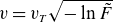 $v = v_T \sqrt {-\ln \tilde {F}}$
and, upon executing the integrals and equating the two, we find that
$v = v_T \sqrt {-\ln \tilde {F}}$
and, upon executing the integrals and equating the two, we find that
 \begin{align} ( {-} \ln \tilde {F} )^{3/2} = \left \langle \left ( \frac {w - \kappa }{T} \right )^{3/2} \right \rangle . \end{align}
The volume average, $\langle \ldots \rangle$
, can readily be evaluated so that the ground state becomes
$\langle \ldots \rangle$
, can readily be evaluated so that the ground state becomes
 \begin{equation} F(w) = M \exp \left \{ - \left [ \frac {1}{2} \mathcal{R} \left ( \frac {w - \kappa _0}{T} \right )^{3/2} + \frac {1}{2} \mathcal{R} \left ( \frac {w - \kappa _1}{T} \right )^{3/2} \right ]^{2/3}\right \}\!. \end{equation}
The available energy as a function of $c$
, calculated in various ways. The solid blue line solves (A6) and (A7). The blue plus-shaped markers solve equation (2.12) of Chen (Reference Chen1966a
) in a modern python framework, whereas the red cross-shaped markers are the reported values in Chen. Finally, the dashed grey line denotes the asymptotic scaling analytically derived in the small
$c$
, calculated in various ways. The solid blue line solves (A6) and (A7). The blue plus-shaped markers solve equation (2.12) of Chen (Reference Chen1966a
) in a modern python framework, whereas the red cross-shaped markers are the reported values in Chen. Finally, the dashed grey line denotes the asymptotic scaling analytically derived in the small $|c|$
limit, whereas the dotted black line is the scaling reported in Chen.
$|c|$
limit, whereas the dotted black line is the scaling reported in Chen.

Figure 11. Long description
The line graph presents the available energy as a function of c, calculated through different methods. The solid blue line represents the solution to equations A6 and A7. Blue plus-shaped markers indicate the solution to equation 2.12 of Chen 1966a using a modern Python framework, while red cross-shaped markers show the reported values from Chen. The dashed grey line denotes the asymptotic scaling analytically derived in the small limit, and the dotted black line represents the scaling reported in Chen.
The scalars $\kappa _0$
and
$\kappa _0$
and $\kappa _1$
are determined by the constraint on the density
$\kappa _1$
are determined by the constraint on the density
 \begin{align} \int \mathrm{d}{\boldsymbol{v}} F[\epsilon +\kappa _0] = n_0(1-c),\nonumber \\ \int \mathrm{d}{\boldsymbol{v}} F[\epsilon +\kappa _1] = n_0(1+c). \end{align}
Given the solutions $\kappa _0$
and
$\kappa _0$
and $\kappa _1$
to these equations, the ground-state energy can readily be determined as
$\kappa _1$
to these equations, the ground-state energy can readily be determined as
 \begin{equation} E_{\mathrm{K,min}} = \frac {1}{2} \int \mathrm{d}{\boldsymbol{x}} \frac {\epsilon }{2} ( F[\epsilon +\kappa _0] + F[\epsilon +\kappa _1] ). \end{equation}
The above equation (A7) can be solved analytically in the small $|c|$
(and correspondingly small
$|c|$
(and correspondingly small $|\kappa |$
) limit, giving rise to
$|\kappa |$
) limit, giving rise to
 \begin{equation} \frac {A}{E_T} = \frac {E_T - E_{\mathrm{K,min}}}{E_T} \approx -\frac {c^2}{3} + \mathcal{O}(c^3). \end{equation}
This is in close, but not exact, agreement with Chen. To investigate the origin of this discrepancy, we have developed a numerical routine in python to solve equation (2.12) of Chen (Reference Chen1966a
). Another routine to numerically solve (A6) and (A7) has been developed too, and we find that these modern routines show excellent agreement, as seen in figure 11. The values for the available energy reported in Chen seem to overestimate the true value in the small $|c|$
limit, following somewhat more closely a
$|c|$
limit, following somewhat more closely a $0.4 c^2$
scaling. We were unable to locate the code used to evaluate the reported values, but from the above considerations we suspect that an outdated or non-converged numerical routine is the culprit of the discrepancy.
$0.4 c^2$
scaling. We were unable to locate the code used to evaluate the reported values, but from the above considerations we suspect that an outdated or non-converged numerical routine is the culprit of the discrepancy.
Appendix B. Nonlinear regimes
As discussed in the main text, in order to maintain a positive-definite number density, the function $\nu$
favours one-dimensional profiles and should thus approach a Dirac-delta distribution in order to increase its magnitude. As such, we perform an investigation of the available energy with two free parameters: the amplitude of the Dirac-delta peak and its ‘structure size’. One parameter can then be used to ensure energetic consistency,
$\nu$
favours one-dimensional profiles and should thus approach a Dirac-delta distribution in order to increase its magnitude. As such, we perform an investigation of the available energy with two free parameters: the amplitude of the Dirac-delta peak and its ‘structure size’. One parameter can then be used to ensure energetic consistency, $A=E_{\phi }$
, so that the remaining parameter maximises the available energy. To make this more precise, we let
$A=E_{\phi }$
, so that the remaining parameter maximises the available energy. To make this more precise, we let $1+\nu (x)$
be the ‘box-car’ function on the domain
$1+\nu (x)$
be the ‘box-car’ function on the domain $x\in [-x_0,x_0]$
, where
$x\in [-x_0,x_0]$
, where $x_0$
is the structure size, defined as
$x_0$
is the structure size, defined as
 \begin{equation} 1+\nu (x) = \begin{cases} \dfrac {x_0}{\sigma } & \text{if } |x|\lt \sigma, \\[8pt] 0 & \text{otherwise}. \end{cases} \end{equation}
Here $\sigma$
measures the width (and amplitude) of the peak, and the function furthermore satisfies
$\sigma$
measures the width (and amplitude) of the peak, and the function furthermore satisfies $\int \mathrm{d}{x} \nu = 0$
. We now require appropriate relations for
$\int \mathrm{d}{x} \nu = 0$
. We now require appropriate relations for $\hat {\phi }$
, which in the case of a neutralising background is simply
$\hat {\phi }$
, which in the case of a neutralising background is simply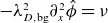 $- \lambda _{D,{\mathrm{bg}}}^2 \partial _x^2 \hat {\phi } = \nu$
. In Fourier space, the field energy can readily be evaluated by noting that the Fourier series of
$- \lambda _{D,{\mathrm{bg}}}^2 \partial _x^2 \hat {\phi } = \nu$
. In Fourier space, the field energy can readily be evaluated by noting that the Fourier series of $\nu$
is equal to
$\nu$
is equal to
 \begin{equation} \nu (x) = 2 \sum _{i=1}^{\infty } \mathrm{sinc}(ik_x\sigma ) \cos (ik_x x), \end{equation}
so that Parseval’s theorem in the small- $\sigma$
limit yields
$\sigma$
limit yields
 \begin{align} E_{\phi } &= E_{\phi ,0} \sum _{i=1}^{\infty } \frac {\mathrm{sinc}^2(ik_x \sigma )}{\big(i \lambda _{D,{\mathrm{bg}}} k_x\big)^2} \nonumber\\ &\approx \frac {E_{\phi ,0} }{6 } \frac {x_0^2}{\lambda _{D,{\mathrm{bg}}}^2}. \end{align}
The available energy thus approaches this constant, where the field energy is maximal for a structure size at the system length $x_0 \sim L$
. Since, for
$x_0 \sim L$
. Since, for $B=0$
, the maximising mode in the linear regime already settles at the longest possible length scale
$B=0$
, the maximising mode in the linear regime already settles at the longest possible length scale $L$
, no additional energy can be freed up by seeking larger structures. In the neutralising case we have thus shown that asymptotically two regimes of the available energy exist: a linear one and one where the constant bound (B3) is approached.
$L$
, no additional energy can be freed up by seeking larger structures. In the neutralising case we have thus shown that asymptotically two regimes of the available energy exist: a linear one and one where the constant bound (B3) is approached.
If the background has a Boltzmann response however, this behaviour is changed due to its damping behaviour. At the critical point where $\nu \leqslant - 1$
, the field amplitude can be calculated using the linearised Boltzmann response, giving
$\nu \leqslant - 1$
, the field amplitude can be calculated using the linearised Boltzmann response, giving
 \begin{equation} \left|\frac {\hat {\phi }_{\boldsymbol{k}}}{\nu _{\boldsymbol{k}}} \right| \sim \frac {1}{ 1 + \sqrt {1 + {E_{\mathrm{bg}}}/{E_{\mathrm{G}}}}} \leqslant \frac {1}{2}. \end{equation}
It is thus appropriate to retain this linearised response even as $\nu$
approaches a Dirac-delta peak, at least up to some critical point where
$\nu$
approaches a Dirac-delta peak, at least up to some critical point where $\hat {\phi } \sim 1$
. This regime is dubbed ‘intermediately nonlinear’ and its scalings are calculated in the following section.
$\hat {\phi } \sim 1$
. This regime is dubbed ‘intermediately nonlinear’ and its scalings are calculated in the following section.
B.1. Intermediately nonlinear
In order to find the energy in the field, one can employ Parseval’s theorem using the Fourier expansion given in (B2), yielding
 \begin{equation} E_{\phi } \approx E_{\phi ,0} \sum _{i=1}^{\infty } \frac { \big(i \lambda _{D,{\mathrm{bg}}} k_x\big)^2 \mathrm{sinc}^2(i k_x \sigma )}{[1+\big(i \lambda _{D,{\mathrm{bg}}} k_x\big)^2]^2}, \end{equation}
and one can calculate its leading order and first-order correction in the smallness of $\sigma$
. Setting
$\sigma$
. Setting $\mathrm{sinc}(ik_x\sigma ) = 1$
and
$\mathrm{sinc}(ik_x\sigma ) = 1$
and $\lambda _{D,{\mathrm{bg}}}k_x=1/y$
, take note of the following sum identity of the hyperbolic cotangent (Gradshteyn & Ryzhik Reference Gradshteyn and Ryzhik2014, § 1.421):
$\lambda _{D,{\mathrm{bg}}}k_x=1/y$
, take note of the following sum identity of the hyperbolic cotangent (Gradshteyn & Ryzhik Reference Gradshteyn and Ryzhik2014, § 1.421):
 \begin{equation} S(y) = \sum _{i=1}^{\infty } \frac {1}{1+( {i}/{y} )^2} = \frac {\pi y \coth (\pi y) - 1}{2} \end{equation}
whose derivative with respect to $y$
is of the desired form
$y$
is of the desired form
 \begin{equation} \frac {S^{\prime} (y) y}{2} = \sum _{i=1}^{\infty } \frac {( {i}/{y} )^2}{[1+( {i}/{y} )^2]^2} = \frac {\pi y}{4} \left [ \frac {\cosh (\pi y) \sinh (\pi y) - \pi y}{\sinh ^2(\pi y)} \right ]\!. \end{equation}
As such the leading-order equation for the field energy is given as
 \begin{equation} E_{\phi }(\sigma \rightarrow 0) \approx \frac {E_{\phi ,0} x_0}{4 \lambda _{D,{\mathrm{bg}}}} \underbrace { \left [ \frac {\cosh (x_0/\lambda _{D,{\mathrm{bg}}}) \sinh (x_0/\lambda _{D,{\mathrm{bg}}}) - x_0/\lambda _{D,{\mathrm{bg}}}}{\sinh ^2(x_0/\lambda _{D,{\mathrm{bg}}})} \right ]}_{\mathcal{F}(x_0/\lambda _{D,{\mathrm{bg}}})} + \,\mathcal{O}(\sigma ). \end{equation}
The higher-order terms involving $\sigma$
require one to evaluate
$\sigma$
require one to evaluate $\Delta E_\phi = E_{\phi }(\sigma ) - E_{\phi }(0)$
, given as
$\Delta E_\phi = E_{\phi }(\sigma ) - E_{\phi }(0)$
, given as
 \begin{equation} \Delta E_\phi = E_{\phi ,0}\sum _{i=1}^{\infty } \frac { ( {i}/{y})^2 }{[ 1 + ({i}/{y} )^2]^2 } [ \mathrm{sinc}^2( i k_x \sigma ) -1 ]. \end{equation}
A straightforward Taylor expansion is insufficient as the sum diverges, since the large argument behaviour of the $\mathrm{sinc}$
function is not accurately captured. By changing the summation index to
$\mathrm{sinc}$
function is not accurately captured. By changing the summation index to $i k_x \sigma = j$
, the sum becomes
$i k_x \sigma = j$
, the sum becomes
 \begin{equation} \Delta E_\phi =E_{\phi ,0} \sum _{j=k_x \sigma }^{\infty } \frac { ( {j}/{y k_x \sigma })^2 }{ [ 1 + ( {j}/{y k_x \sigma } )^2]^2 } [ \mathrm{sinc}^2( j) -1 ], \end{equation}
where $j$
contains all positive integer multiples of
$j$
contains all positive integer multiples of $ k_x \sigma$
. The limit
$ k_x \sigma$
. The limit $\sigma \rightarrow 0$
may now be taken where, due to the infinitesimally small distance between consecutive evaluation points, the sum approaches the integral
$\sigma \rightarrow 0$
may now be taken where, due to the infinitesimally small distance between consecutive evaluation points, the sum approaches the integral
 \begin{align} \Delta E_\phi &\approx \frac {E_{\phi ,0} \sigma }{\lambda _{D,{\mathrm{bg}}}^2 k_x } \int _0^{\infty } \frac { \mathrm{sinc}^2( j) -1 }{j^2 } \mathrm{d} j \nonumber\\ &\approx -\frac {E_{\phi ,0} x_0^2 }{3\lambda _{D,{\mathrm{bg}}}^2 } \frac {\sigma }{x_0}. \end{align}
The energetic penalty of the background need only be evaluated to leading order. Parseval’s theorem yields
 \begin{align} A_{\mathrm{bg}} &\approx - E_{\mathrm{bg}} \frac {d+2}{d^2} \sum _{i=1}^{\infty } \frac {1}{[1+\big(i \lambda _{D,{\mathrm{bg}}} k_x\big)^2]^2} \nonumber\\ &\approx - \frac {E_{\mathrm{bg}}}{4} \frac {d+2}{d^2} \frac {x_0}{\lambda _{D,{\mathrm{bg}}}} \underbrace {\left [ \frac {\cosh (x_0/\lambda _{D,{\mathrm{bg}}})}{\sinh (x_0/\lambda _{D,{\mathrm{bg}}})} - \frac {2\lambda _{D,{\mathrm{bg}}}}{x_0} + \frac {x_0}{\lambda _{D,{\mathrm{bg}}} \sinh ^2(x_0/\lambda _{D,{\mathrm{bg}}})} \right ]}_{\mathcal{B}(x_0/\lambda _{D,{\mathrm{bg}}})}, \end{align}
and we can now evaluate the available energy. Energetic consistency requires that
 \begin{align} A_{\mathrm{G}} - E_{\mathrm{G}} \left ( \frac {x_0}{\sigma } \right )^{2/d} - \frac {E_{\mathrm{bg}}}{4} \frac {d+2}{d^2} \frac {x_0}{\lambda _{D,{\mathrm{bg}}}} \mathcal{B}\left ( \frac {x_0}{\lambda _{D,{\mathrm{bg}}}} \right ) = \frac {E_{\phi ,0} x_0}{4 \lambda _{D,{\mathrm{bg}}}} \left [ \mathcal{F} \left ( \frac {x_0}{\lambda _{D,{\mathrm{bg}}}} \right ) - \frac {4}{3} \frac {x_0}{ \lambda _{D,{\mathrm{bg}}}} \frac {\sigma }{x_0} \right ]\!.\nonumber\\[-10pt]\nonumber\\ \end{align}
For $d=1$
, to leading order in the smallness of
$d=1$
, to leading order in the smallness of $\sigma$
, we must have
$\sigma$
, we must have
 \begin{equation} \frac {\sigma }{x_0} \approx \sqrt { \frac {E_{\mathrm{G}}}{A_{\mathrm{G}}}}, \end{equation}
giving rise to a field energy
 \begin{equation} E_{\phi } \approx \frac {E_{\phi ,0}}{4} \left ( \frac {x_0}{\lambda _{D,{\mathrm{bg}}}} - \frac {4}{3} \frac {x_0^2}{ \lambda _{D,{\mathrm{bg}}}^2} \sqrt {\frac {E_{\mathrm{G}}}{A_{\mathrm{G}}}} \right )\!, \end{equation}
where we have used the large argument expansion $\mathcal{F}(x_0/\lambda _{D,{\mathrm{bg}}}) \approx 1$
. This is maximal for a structure size
$\mathcal{F}(x_0/\lambda _{D,{\mathrm{bg}}}) \approx 1$
. This is maximal for a structure size
 \begin{equation} \frac {x_0}{\lambda _{D,{\mathrm{bg}}}} \approx \frac {3}{8} \sqrt {\frac {A_{\mathrm{G}}}{E_{\mathrm{G}}}}, \end{equation}
and the available energy to leading order becomes
 \begin{equation} A \approx \frac {3E_{\phi ,0}}{64} \sqrt {\frac {A_{\mathrm{G}}}{E_{\mathrm{G}}}}. \end{equation}
We observe that the ground state with a linearised Boltzmann response seeks larger structure sizes, and has a sublinear scaling with $A_{\mathrm{G}}$
. In cases where
$A_{\mathrm{G}}$
. In cases where $d\geqslant 2$
, the equation can be satisfied by
$d\geqslant 2$
, the equation can be satisfied by $x_0/\sigma \propto A_{\mathrm{G}}^{d/2}$
, where, furthermore, setting
$x_0/\sigma \propto A_{\mathrm{G}}^{d/2}$
, where, furthermore, setting $x_0 / \lambda _{D,{\mathrm{bg}}} \propto A_{\mathrm{G}}$
allows one to solve for the proportionality constants (using the large argument limit
$x_0 / \lambda _{D,{\mathrm{bg}}} \propto A_{\mathrm{G}}$
allows one to solve for the proportionality constants (using the large argument limit $\mathcal{B}(x_0/ \lambda _{D,{\mathrm{bg}}}) \approx 1$
). As such, the field energy goes to
$\mathcal{B}(x_0/ \lambda _{D,{\mathrm{bg}}}) \approx 1$
). As such, the field energy goes to $E_{\phi } \propto A_{\mathrm{G}}$
and a linear scaling of the available energy persists in this intermediately nonlinear regime for
$E_{\phi } \propto A_{\mathrm{G}}$
and a linear scaling of the available energy persists in this intermediately nonlinear regime for $d \geqslant 2$
.
$d \geqslant 2$
.
B.2 Strongly nonlinear
As $\hat {\phi }$
increases in value, we enter a new nonlinear regime where the full Boltzmann response must be retained. In order to find approximate expressions for the field energy and the background penalty we require a solution of the Poisson–Boltzmann equation,
$\hat {\phi }$
increases in value, we enter a new nonlinear regime where the full Boltzmann response must be retained. In order to find approximate expressions for the field energy and the background penalty we require a solution of the Poisson–Boltzmann equation,
 \begin{equation} -\lambda _{D,{\mathrm{bg}}}^2 \hat {\phi }^{\prime\prime}(x) +{\rm e}^{\hat {\phi }(x)} = 1+ \nu (x), \end{equation}
which can be done in the case that $1 + \nu$
approaches a Dirac-delta distribution. Starting from (B18), we first integrate across the origin where the source approaches a Dirac delta. Hence, for sufficiently small
$1 + \nu$
approaches a Dirac-delta distribution. Starting from (B18), we first integrate across the origin where the source approaches a Dirac delta. Hence, for sufficiently small $\varepsilon$
,
$\varepsilon$
,
 \begin{align} -\lambda _{D,{\mathrm{bg}}}^2 \int _{-\varepsilon }^{\varepsilon } \mathrm{d}{x}\, \hat {\phi }^{\prime\prime}(x) + \int _{-\varepsilon }^{\varepsilon } \mathrm{d}{x}\, {\rm e}^{\hat {\phi }(x)} = 2 x_0 \int _{-\varepsilon }^{\varepsilon } \mathrm{d}{x}\, \delta (x) \implies \hat {\phi }^{\prime} (-\varepsilon ) - \hat {\phi }^{\prime} (\varepsilon ) = \frac {2x_0}{\lambda _{D,{\mathrm{bg}}}^2},\nonumber\\[-10pt]\nonumber\\ \end{align}
and we see there is a sharp discontinuity in the electric field at the origin, where evenness of the function implies that $-\hat {\phi }^{\prime} (0^{-})= \hat {\phi }^{\prime} (0^+) = -x_0/\lambda _{D,{\mathrm{bg}}}^2$
. Further multiplying the Poisson–Boltzmann equation by
$-\hat {\phi }^{\prime} (0^{-})= \hat {\phi }^{\prime} (0^+) = -x_0/\lambda _{D,{\mathrm{bg}}}^2$
. Further multiplying the Poisson–Boltzmann equation by $\hat {\phi }^{\prime} (x)$
allows one to convert the equation to a first-order nonlinear ordinary differential equation,
$\hat {\phi }^{\prime} (x)$
allows one to convert the equation to a first-order nonlinear ordinary differential equation,
 \begin{equation} \frac {\mathrm{d}}{\mathrm{d}x} ( \hat {\phi }^{\prime} (x)^2 ) = \frac {\mathrm{d}}{\mathrm{d}x}\left ( \frac {2{\rm e}^{\hat {\phi }(x)} }{\lambda _{D,{\mathrm{bg}}}^2} \right ) \implies \hat {\phi }^{\prime} (x) = \pm \sqrt {\frac {2{\rm e}^{\hat {\phi }(x)}}{\lambda _{D,{\mathrm{bg}}}^2} - C_0}. \end{equation}
Focusing on the decreasing solution, it is useful to apply the substitution $\varPhi = \exp (\hat {\phi })$
, so that the equation becomes
$\varPhi = \exp (\hat {\phi })$
, so that the equation becomes
 \begin{equation} \varPhi ^{\prime} (x) = - \frac {\varPhi (x)\sqrt {2}}{\lambda _{D,{\mathrm{bg}}}} \sqrt {\varPhi (x)-\varPhi _b}, \end{equation}
where $\varPhi _b$
is the value of
$\varPhi _b$
is the value of $\varPhi$
at the periodic boundary
$\varPhi$
at the periodic boundary $x_0$
, thus,
$x_0$
, thus, $\varPhi ^{\prime} (x_0) = 0$
. The separation of variables yields
$\varPhi ^{\prime} (x_0) = 0$
. The separation of variables yields
 \begin{align} & \arctan \left ( \sqrt {\frac {\varPhi }{\varPhi _b} - 1} \right ) = -\frac {x }{\lambda _{D,{\mathrm{bg}}}} \sqrt {\frac {\varPhi _b}{2}} + C_1 + \frac {\pi }{2} \nonumber\\&\quad \implies \varPhi (x) = \varPhi _b \sin ^{-2} \left ( \frac {x}{\lambda _{D,{\mathrm{bg}}}} \sqrt {\frac {\varPhi _b}{2}} +C_1 \right )\!. \end{align}
We denote the central value as $\varPhi (0)=\varPhi _0$
, so that
$\varPhi (0)=\varPhi _0$
, so that $C_1$
is determined by
$C_1$
is determined by
 \begin{equation} C_1 = \arcsin \left ( \sqrt {\frac {\varPhi _b}{\varPhi _0}} \right ), \end{equation}
and the value $\varPhi _b$
is set by the transcendental equation
$\varPhi _b$
is set by the transcendental equation
 \begin{equation} \frac {x_0}{\lambda _{D,{\mathrm{bg}}}} \sqrt {\frac {\varPhi _b}{2}} + C_1 = \frac {\pi }{2}. \end{equation}
The edge and centre values are coupled via $\hat {\phi }^{\prime} (0^+) = -x_0/\lambda _{D,{\mathrm{bg}}}^2$
, giving
$\hat {\phi }^{\prime} (0^+) = -x_0/\lambda _{D,{\mathrm{bg}}}^2$
, giving
 \begin{equation} \varPhi _0 = \varPhi _b + \frac {x_0^2}{2\lambda _{D,{\mathrm{bg}}}^2}, \end{equation}
showing that the edge contribution becomes negligible for $x_0/\lambda _{D,{\mathrm{bg}}} \gg 1$
due to the Debye shielding, which furthermore increases the potential strength leading to stronger field energy. Equations (B22)–(B25) solve the Poisson–Boltzmann equation in general with a Dirac-delta source with periodic boundary conditions. It furthermore allows one to evaluate the field energy, which becomes
$x_0/\lambda _{D,{\mathrm{bg}}} \gg 1$
due to the Debye shielding, which furthermore increases the potential strength leading to stronger field energy. Equations (B22)–(B25) solve the Poisson–Boltzmann equation in general with a Dirac-delta source with periodic boundary conditions. It furthermore allows one to evaluate the field energy, which becomes
 \begin{equation} E_{\phi } = 2 E_{\phi ,0}\left \{1 - \frac {\sqrt {2\varPhi _b}}{X} \left [ \frac {\pi }{2} - \arctan \left ( \frac {\sqrt {2\varPhi _b}}{X} \right ) \right ] \right \}\!, \end{equation}
having defined $X = x_0/\lambda _{D,{\mathrm{bg}}}$
. The boundary value depends on
$X = x_0/\lambda _{D,{\mathrm{bg}}}$
. The boundary value depends on $X$
via
$X$
via
 \begin{equation} X \sqrt {\frac {\varPhi _b}{2}} + \arcsin \left ( \sqrt {\frac {2\varPhi _b}{2\varPhi _b + X^2}} \right ) = \frac {\pi }{2}, \end{equation}
which in the large $X$
limit becomes
$X$
limit becomes
 \begin{equation} \varPhi _b \approx \frac {\pi ^2}{2 X^2}. \end{equation}
The maximal field energy is thus attained by letting $X \rightarrow \infty$
, giving
$X \rightarrow \infty$
, giving
 \begin{equation} E_{\phi } \approx 2 E_{\phi ,0} + \mathcal{O}(X^{-2}). \end{equation}
B.3. Verification
The available energy of the single-waterbag distribution function as a function of $A_{\mathrm{G}}$
. Here
$A_{\mathrm{G}}$
. Here $\lambda _{D,{\mathrm{bg}}} = E_{\mathrm{G}} = E_{\phi ,0} = E_{\mathrm{bg}} = 1$
and the domain is taken to be
$\lambda _{D,{\mathrm{bg}}} = E_{\mathrm{G}} = E_{\phi ,0} = E_{\mathrm{bg}} = 1$
and the domain is taken to be $x \in [0,6 \pi )$
. Scalings are added for the linear regime (dashed), the intermediately nonlinear regime (dotted) and the strict upper bound (dash-dotted). Finally, the critical Gardner energy where the constraint of positive definiteness becomes important is added as a solid grey line.
$x \in [0,6 \pi )$
. Scalings are added for the linear regime (dashed), the intermediately nonlinear regime (dotted) and the strict upper bound (dash-dotted). Finally, the critical Gardner energy where the constraint of positive definiteness becomes important is added as a solid grey line.

Figure 12. Long description
A line graph showing the available energy of the single-waterbag distribution function as a function of A G. The x axis represents A G on a logarithmic scale ranging from 10 to the power of negative 1 to 10 to the power of 2. The y axis represents A on a logarithmic scale ranging from 10 to the power of negative 2 to 10 to the power of 0. The graph includes multiple lines representing different scalings: a dashed line for the linear regime, a dotted line for the intermediately nonlinear regime, a dash-dotted line for the strict upper bound, and a solid grey line for the critical Gardner energy. The data points are marked with black crosses.
We finally numerically verify found scalings, where we maximise the available energy subject to the constraints for $d=1$
(for numerical details, see Appendix D). The result is shown in figure 12: there is excellent agreement in the linear regime and one can clearly see the available energy decrease markedly when the constraint of positive definiteness becomes relevant (
$d=1$
(for numerical details, see Appendix D). The result is shown in figure 12: there is excellent agreement in the linear regime and one can clearly see the available energy decrease markedly when the constraint of positive definiteness becomes relevant ( $A_{\mathrm{G}} \sim A_{\mathrm{ph}}$
). The upper bound is not reached even at
$A_{\mathrm{G}} \sim A_{\mathrm{ph}}$
). The upper bound is not reached even at $A_{\mathrm{G}} = 10^2$
and going beyond this regime likely requires exceedingly high resolution, at least with the current numerical methods.
$A_{\mathrm{G}} = 10^2$
and going beyond this regime likely requires exceedingly high resolution, at least with the current numerical methods.
Appendix C. Linear analysis of the two-stream waterbag instability
To gain further insight into the results of the simulations given in § 3.4, we perform a linear analysis of the single-waterbag two-stream instabilities in one dimension, in the case of a neutralising and adiabatic (i.e. $n_{\mathrm{bg}} \propto \phi$
) background. To this end, let us describe the waterbag as
$n_{\mathrm{bg}} \propto \phi$
) background. To this end, let us describe the waterbag as
 \begin{equation} f_0(v) = \frac {n_0}{2 \Delta } \left ( \varTheta \left [ \frac {\varDelta }{2} - |v - v_0| \right ] + \varTheta \left [ \frac {\varDelta }{2} - |v + v_0| \right ] \right )\!, \end{equation}
where we refer to figure 1 for definitions of the different quantities. The linearised Vlasov equation ( $f = f_0 + \varepsilon f$
and
$f = f_0 + \varepsilon f$
and $\phi = \varepsilon \phi$
, keeping only terms of order
$\phi = \varepsilon \phi$
, keeping only terms of order $\varepsilon$
) in Fourier space, where the foreground species has charge
$\varepsilon$
) in Fourier space, where the foreground species has charge $q$
and mass
$q$
and mass $m$
, yields
$m$
, yields
 \begin{equation} \varepsilon f_k = -\frac {q}{m} \frac {k f_0^{\prime} (v)}{\omega - k v} \varepsilon \phi _k, \end{equation}
where we realise that $f_0^{\prime} (v)$
consists of four Dirac-delta peaks at the edges of the waterbag. As such, the perturbed density is given as
$f_0^{\prime} (v)$
consists of four Dirac-delta peaks at the edges of the waterbag. As such, the perturbed density is given as
 \begin{equation} \varepsilon n_k = \frac {\epsilon _0 \varepsilon \phi _k}{q} \frac {\omega _p^2 k^2}{2} \left ( \frac {1}{\varOmega _+^2} + \frac {1}{\varOmega _-^2} \right )\!, \end{equation}
having defined the plasma frequency $\omega _p^2 = q^2 n_0 / m \epsilon _0$
and the frequencies
$\omega _p^2 = q^2 n_0 / m \epsilon _0$
and the frequencies $\varOmega _{\pm }^2=(\omega \pm kv_0)^2 - k^2 (\varDelta /2)^2$
. This can be coupled to the Poisson equation,
$\varOmega _{\pm }^2=(\omega \pm kv_0)^2 - k^2 (\varDelta /2)^2$
. This can be coupled to the Poisson equation,
 \begin{equation} k^2 \varepsilon \phi _k = \frac { q}{\epsilon _0} ( \varepsilon n_k - \varepsilon n_{k,\mathrm{bg}} ), \end{equation}
where the background density ( $\varepsilon n_{\mathrm{bg}}= B q n_0 \varepsilon \phi / T_{\mathrm{bg}}$
) can be neutralising (
$\varepsilon n_{\mathrm{bg}}= B q n_0 \varepsilon \phi / T_{\mathrm{bg}}$
) can be neutralising ( $B=0$
) or adiabatic (
$B=0$
) or adiabatic ( $B=1$
). Poisson’s equation becomes
$B=1$
). Poisson’s equation becomes
 \begin{equation} \frac {\omega _p^2}{2}\left ( \frac {1}{\varOmega _+^2} + \frac {1}{\varOmega _-^2} \right ) = 1+\frac {B}{\lambda _{D,\mathrm{bg}}^2 k^2}, \end{equation}
which can be rewritten as a quadratic equation in $\omega ^2$
. This can be solved exactly, where the wavenumber that maximises the growth rate satisfies
$\omega ^2$
. This can be solved exactly, where the wavenumber that maximises the growth rate satisfies
 \begin{equation} \lambda _{D,\mathrm{bg}}^2k_{\mathrm{max}}^2 = \omega _p^2 \lambda _{B,\mathrm{bg}}^2 \frac {4 v_0^2 + \varDelta ^2 -2v_0\sqrt {4v_0^2 - \varDelta ^2}}{2 v_0 \varDelta ^2\sqrt {4v_0^2 - \varDelta ^2}} - B . \end{equation}
Next, we focus on the energy in the electric field and relate it to the density fluctuations:
 \begin{equation} E_{\phi } = \frac {\epsilon _0}{2} \int \mathrm{d}{k} 2 \pi k^2 |\varepsilon \phi _k|^2 = \frac {n_0 T_{\mathrm{bg}}}{2} \int \mathrm{d}{k} 2\pi \left |\frac {\varepsilon n_k}{n_0} \right |^2 \frac {\lambda _{D,\mathrm{bg}}^2 k^2}{\big(\lambda _{D,\mathrm{bg}}^2 k^2+B\big)^2} .\end{equation}
Evidently, in the linear phase, $k_{\mathrm{max}}$
will dominate, so that the relationship between the energy in the electric field and the density fluctuations becomes
$k_{\mathrm{max}}$
will dominate, so that the relationship between the energy in the electric field and the density fluctuations becomes
 \begin{align} E_{\phi } &= \frac {n_0 T_{\mathrm{bg}} V}{2} \frac {\lambda _{D,\mathrm{bg}}^2 k_{\mathrm{max}}^2}{\big(\lambda _{D,\mathrm{bg}}^2 k_{\mathrm{max}}^2+B\big)^2} \left \langle \left ( \frac {\varepsilon n (x)}{n_0} \right )^2 \right \rangle . \end{align}
Here we see clearly that, for increasing fluctuation level, energy is being pumped into the electric field, in contrast to the result for a ground state. This is qualitatively in line with the result of figure 6, where for increasing density fluctuations, we see a decrease in the thermal energy of the waterbag and, thus, an increase in the field energy.
Let us verify the predicted scaling with the simulations, seeing how closely the results adhere to it. The result of this analysis is plotted in figure 13, where we see that the simulation results are somewhat well described by the linear picture in the neutralising case and fairly well described in the kinetic case. It is furthermore interesting to observe that there is an apparent upper bound on the relation between the density fluctuations and the electric-field energy in the kinetic case, but not so for the neutralising case. This is readily understood from (C8): for $B=1$
, one can show that
$B=1$
, one can show that $E_{\phi } \leqslant n_0 T_{\mathrm{bg}} V \langle (\varepsilon n/n_0 )^2 \rangle /8$
. For the neutralising case (
$E_{\phi } \leqslant n_0 T_{\mathrm{bg}} V \langle (\varepsilon n/n_0 )^2 \rangle /8$
. For the neutralising case ( $B=0$
) however, no such bound can be constructed as the proportionality constant can be made arbitrarily large as
$B=0$
) however, no such bound can be constructed as the proportionality constant can be made arbitrarily large as $k\rightarrow 0$
: as lower wavenumbers are activated, more energy can be pumped into the electric field.
$k\rightarrow 0$
: as lower wavenumbers are activated, more energy can be pumped into the electric field.
Scatter plot of the energy in the electric field and the density fluctuations, multiplied by the proportionality constant given by linear theory, for all the simulations given in § 3.4 (i.e. with a neutralising and kinetic background). The dark colours (initial times) collapse onto the same line, as expected. At later times, the scalings still work reasonably well, though certainly deviating.

Figure 13. Long description
A scatter plot representing the relationship between the energy in the electric field and the density fluctuations, multiplied by a proportionality constant from linear theory. The plot includes data from simulations with both neutralising and kinetic backgrounds. Darker colors indicate initial times, and these data points collapse onto the same line as expected. At later times, the scalings still hold reasonably well but show some deviation. The x-axis represents the product of the squared density fluctuations and a proportionality constant, while the y-axis represents the squared gradient of the electric field. The data points are color-coded based on the ratio of time to maximum time, ranging from 0 to 1. The plot shows a positive correlation between the variables, with some spread in the data at later times.
Appendix D. Numerical scheme for the single-waterbag ground state
Here we detail how the code calculates the ground state of a single-waterbag distribution function in one dimension. We remind ourselves that we wish to achieve the following.
-
(i) Maximise the available energy,
(D1)where
\begin{equation} A = A_{\mathrm{G}} - E_{\mathrm{G}}\langle [1 + \nu (x) ]^{({d+2})/{d}} - 1 \rangle - E_{\mathrm{bg}} \langle [1 + \nu _{\mathrm{bg}}(x) ]^{({d+2})/{d}} - 1 \rangle , \end{equation}
$\nu$
relates to the density perturbation as
$\delta n(x) / n_0 = \nu$
and similarly for the background density, which related to the electric field via the Boltzmann response,
$\nu _{\mathrm{bg}} = \exp (\hat {\phi }) - 1$
. The background response may also be set to zero, in case it is neutralising.
-
(ii) Ensure the electric field has the appropriate energetic content, i.e.
(D2)where the electric field satisfies the Poisson–Boltzmann equation
\begin{equation} A = E_\phi , \end{equation}
$- \lambda _{D,{\mathrm{bg}}}^2 \partial _x^2 \hat {\phi } + e^{\hat {\phi }} -1 =\nu$
or the neutral response
$\lambda _{D,{\mathrm{bg}}}^2 \boldsymbol{\nabla} ^2 \hat {\phi } = \nu$
.
-
(iii) The number density must be positive, i.e.
(D3)or in terms of the perturbed density one must satisfy
\begin{equation} n(x)\geqslant 0, \end{equation}
$1 + \nu \geqslant 0$
. The background-species density is always positive with a Boltzmann response.
-
(iv) The total number of particles is conserved, i.e.
(D4)or equivalently,
\begin{equation} \int \mathrm{d} x \; \delta n(x) = 0, \end{equation}
$\int \mathrm{d} x \; \nu = 0$
. Note that the background density perturbation automatically preserves particle number due to the Poisson–Boltzmann equation with periodic boundary conditions.





The problem is discretised by representing the density perturbation as a cosine series, i.e.
 \begin{equation} \nu = \sum _{n=1}^{N_{\mathrm{modes}}} c_n \cos\ ( k_x x ), \end{equation}
where $k_x = 2\pi / x_0$
, with
$k_x = 2\pi / x_0$
, with $x_0$
being the domain size so that
$x_0$
being the domain size so that $x \in [0,x_0)$
. Note that this representation automatically ensures that the total particle number is satisfied. In order to numerically solve the problem penalty functions are defined, where energetic consistency is penalised as
$x \in [0,x_0)$
. Note that this representation automatically ensures that the total particle number is satisfied. In order to numerically solve the problem penalty functions are defined, where energetic consistency is penalised as
 \begin{equation} P_1 = \left | \frac {A - E_\phi }{A} \right |. \end{equation}
Negative values of the number density are penalised by calculating the volume-averaged negative contribution to the total number density, i.e.
 \begin{equation} P_2 = \left \langle \mathcal{R} \left [ -\frac {n(x)}{n_0} \right ] \right \rangle , \end{equation}
where $\mathcal{R}$
denotes the ramp function and
$\mathcal{R}$
denotes the ramp function and $P_2$
is non-zero if
$P_2$
is non-zero if $n(x) \lt 0$
, assuming that
$n(x) \lt 0$
, assuming that $n(x)$
is well behaved. We may thus construct the following total penalty function:
$n(x)$
is well behaved. We may thus construct the following total penalty function:
 \begin{equation} J = -A + w_1 P_1^2 + w_2 P_2^2. \end{equation}
Additionally, we wish to find the set $\{ c_n \}$
that minimises
$\{ c_n \}$
that minimises $J$
. By setting the weights
$J$
. By setting the weights $w_1$
and
$w_1$
and $w_2$
sufficiently high,
$w_2$
sufficiently high, $A$
is then maximised subject to constraints, where we have found that setting
$A$
is then maximised subject to constraints, where we have found that setting $w_1 = w_2 = 10^5$
typically works well, and subsequent minimisation is performed with the Broyden–Fletcher–Goldfarb–Shanno algorithm.
$w_1 = w_2 = 10^5$
typically works well, and subsequent minimisation is performed with the Broyden–Fletcher–Goldfarb–Shanno algorithm.
To ensure we are tracking a solution consistently in figure 12, we first solve the problem in the linear regime with $A_{\mathrm{G}} \ll E_{\mathrm{G}}$
after which we ‘adiabatically’ increase the Gardner bound. For each slightly increased value of
$A_{\mathrm{G}} \ll E_{\mathrm{G}}$
after which we ‘adiabatically’ increase the Gardner bound. For each slightly increased value of $A_{\mathrm{G}}$
, the optimisation problem is initialised with its prior solution, and it remains to choose the initialisation in the linear regime. The optimisation problem has multiple local minima in this regime (which can become the global minimum in the nonlinear regime), and thus, depends sensitively on initial conditions. For a given dominant
$A_{\mathrm{G}}$
, the optimisation problem is initialised with its prior solution, and it remains to choose the initialisation in the linear regime. The optimisation problem has multiple local minima in this regime (which can become the global minimum in the nonlinear regime), and thus, depends sensitively on initial conditions. For a given dominant $c_n$
in the initial condition, this
$c_n$
in the initial condition, this $c_n$
typically remains dominant and, as such, we initialise the linear regime with varying dominant modes.
$c_n$
typically remains dominant and, as such, we initialise the linear regime with varying dominant modes.
For figure 4, we use a different solution strategy more appropriate for varying $A_{\mathrm{G}}$
,
$A_{\mathrm{G}}$
, $E_{\mathrm{G}}$
,
$E_{\mathrm{G}}$
, $E_{\mathrm{bg}}$
and
$E_{\mathrm{bg}}$
and $E_{\phi ,0}$
simultaneously. The mode is initialised according to the linear theory, i.e. a monochromatic initial condition where the non-zero wavenumber is given as
$E_{\phi ,0}$
simultaneously. The mode is initialised according to the linear theory, i.e. a monochromatic initial condition where the non-zero wavenumber is given as $\lambda _{D,{\mathrm{bg}}} k_0 = (1+E_{\mathrm{bg}}/E_{\mathrm{G}})^{1/4}$
. The optimisation is initially solved for a low number of modes, where new (zero-amplitude) modes are added and the optimisation is restarted with the initial condition being set by the lower-resolution solution, a similar strategy as employed in Landreman, Medasani & Zhu (Reference Landreman, Medasani and Zhu2021). This leaves open the question to whether initialising with a different monochromatic mode could lead to higher available energies in the nonlinear regime, a computationally expensive task. However, seeing that our found solution does not deviate strongly from the linear result in figure 4, we expect that such corrections, if present, are small and do not alter the results.
$\lambda _{D,{\mathrm{bg}}} k_0 = (1+E_{\mathrm{bg}}/E_{\mathrm{G}})^{1/4}$
. The optimisation is initially solved for a low number of modes, where new (zero-amplitude) modes are added and the optimisation is restarted with the initial condition being set by the lower-resolution solution, a similar strategy as employed in Landreman, Medasani & Zhu (Reference Landreman, Medasani and Zhu2021). This leaves open the question to whether initialising with a different monochromatic mode could lead to higher available energies in the nonlinear regime, a computationally expensive task. However, seeing that our found solution does not deviate strongly from the linear result in figure 4, we expect that such corrections, if present, are small and do not alter the results.
Appendix E. A special property of the Maxwellian
Here we derive the distribution function that has no available energy, given that the density profile has to remain fixed and there is no additional source of free energy (e.g. temperature gradients). Under these conditions the distribution function can be expressed as
 \begin{equation} f(\boldsymbol{x}) = n(\boldsymbol{x}) G[\epsilon (\boldsymbol{x})], \end{equation}
where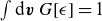 $ \int \mathrm{d}{\boldsymbol{v}}\,G[\epsilon ]=1$
and
$ \int \mathrm{d}{\boldsymbol{v}}\,G[\epsilon ]=1$
and $G^{\prime} (\epsilon ) \leqslant 0$
, automatically satisfying
$G^{\prime} (\epsilon ) \leqslant 0$
, automatically satisfying $\int \mathrm{d}{\boldsymbol{v}}\, f = n(\boldsymbol{x})$
. Set
$\int \mathrm{d}{\boldsymbol{v}}\, f = n(\boldsymbol{x})$
. Set $n(\boldsymbol{x}) =n_0(1+\nu )$
, so that the ground-state equation (upon choosing
$n(\boldsymbol{x}) =n_0(1+\nu )$
, so that the ground-state equation (upon choosing $\langle \nu \rangle = 0$
and
$\langle \nu \rangle = 0$
and $\nu = \tilde {\nu }$
) becomes
$\nu = \tilde {\nu }$
) becomes
 \begin{equation} F_1 = \frac {C f_0 G^{\prime} (\epsilon )}{G(\epsilon )}, \end{equation}
where $C$
is some unknown constant, and this expression may be used to find the available energy. Substituting these results yields
$C$
is some unknown constant, and this expression may be used to find the available energy. Substituting these results yields
 \begin{align} A &\approx -\frac {1}{2} \int \mathrm{d}{\boldsymbol{x}} \frac {f_0^2 \nu ^2}{ F_0^{\prime} } + \frac {1}{2} \int \mathrm{d}{\boldsymbol{r}} \frac {\langle f_0 \rangle _{\boldsymbol{v}}^2 \nu ^2}{\langle F_0^{\prime} \rangle _{\boldsymbol{v}}} \nonumber\\ & \approx \frac {1}{2} \int \mathrm{d}{\boldsymbol{r}} \left ( \left \langle \frac {f_0^2 }{|F_0^{\prime} |} \right \rangle _{\boldsymbol{v}} - \frac {\langle f_0 \rangle _{\boldsymbol{v}}^2 }{\langle |F_0^{\prime} | \rangle _{\boldsymbol{v}}} \right ) \nu ^2. \end{align}
Equation (E3) is always positive definite, as the factor in parentheses is greater than or equal to zero as a consequence of Titu’s lemma (also called Sedrakyan’s inequality or Engel’s form, although ultimately it follows from the Cauchy–Schwarz inequality as discussed in Sedrakyan & Sedrakyan Reference Sedrakyan and Sedrakyan2018, Chapter 8). Titu’s lemma furthermore states that the expression is zero if and only if $-F_0^{\prime} \propto f_0$
, meaning the ground state is Maxwellian.
$-F_0^{\prime} \propto f_0$
, meaning the ground state is Maxwellian.
Consequently, we have shown that in the absence of additional invariants ( $\boldsymbol{y} = \varnothing$
), the Maxwellian is the only distribution function that has vanishing available energy, given that all spatial variation is due to the number density profile and this is furthermore held fixed, and to leading order in closeness to the ground state. Since further constraining the ground state by adding additional invariants can only lower the available energy, it must therefore remain zero for any
$\boldsymbol{y} = \varnothing$
), the Maxwellian is the only distribution function that has vanishing available energy, given that all spatial variation is due to the number density profile and this is furthermore held fixed, and to leading order in closeness to the ground state. Since further constraining the ground state by adding additional invariants can only lower the available energy, it must therefore remain zero for any $\boldsymbol{y}$
to this order. Note that the converse is not necessarily true: zero available energy does not automatically imply that
$\boldsymbol{y}$
to this order. Note that the converse is not necessarily true: zero available energy does not automatically imply that $f$
is a Maxwellian for any
$f$
is a Maxwellian for any $\boldsymbol{y}$
if all spatial variation is due to the density, which is furthermore held fixed.
$\boldsymbol{y}$
if all spatial variation is due to the density, which is furthermore held fixed.
The initial two-waterbag state with varying density (left), the corresponding Gardner state (middle) and the ground state with fixed density (right).

Figure 14. Long description
The image contains three graphs side by side. The first graph on the left shows the initial two-waterbag state with varying density, where the function f_i(x, v_x) is plotted against x and v_x. The graph is divided into two regions, one with f = η2 and the other with f = η1. The middle graph represents the Gardner state, showing F_G(x, v_x) plotted against x and v_x. This graph features horizontal bands indicating different values of the function. The third graph on the right illustrates the ground state with fixed density, displaying F(x, v_x) against x and v_x. This graph includes labeled sections with a, b, c/2, and d/2, indicating specific regions and their respective values. The graphs collectively demonstrate the mapping from an initial state to the Gardner state and to the ground state, highlighting the changes in phase-space.
It is insightful to see a restacking process that gives rise to this available energy, which is most easily done by using a two-waterbag model for the distribution function, further allowing us to probe the nonlinear regime where the density variation may be large. Such a distribution takes on only three values: zero, $\eta _1$
and
$\eta _1$
and $\eta _2$
(where
$\eta _2$
(where $\eta _1\lt \eta _2$
), in line with (E1). We assume the distribution function has density
$\eta _1\lt \eta _2$
), in line with (E1). We assume the distribution function has density $n_1 \propto \eta _1$
in half of the volume and density
$n_1 \propto \eta _1$
in half of the volume and density $n_2 \propto \eta _2$
in the remaining half. A clarifying plot of the initial state is given in the left panel of figure 14. Its corresponding Gardner state is given in the middle panel. A ground state that keeps the density fixed can be constructed by allowing the width of both to vary, as in the third panel. The correct widths
$n_2 \propto \eta _2$
in the remaining half. A clarifying plot of the initial state is given in the left panel of figure 14. Its corresponding Gardner state is given in the middle panel. A ground state that keeps the density fixed can be constructed by allowing the width of both to vary, as in the third panel. The correct widths $\{ a,b,c,d \}$
in this panel are calculated by realising that the Casimirs of both waterbags have to be conserved.Footnote
11
It is further required that the densities are held fixed, and this gives a total of three relationships:
$\{ a,b,c,d \}$
in this panel are calculated by realising that the Casimirs of both waterbags have to be conserved.Footnote
11
It is further required that the densities are held fixed, and this gives a total of three relationships:
 \begin{align} a + b = c+d, \quad a\eta _2 + c \eta _1 = \Delta \eta _2, \quad b \eta _2 + d \eta _1 = \Delta \eta _1. \end{align}
The energy associated with this ground state is furthermore
 \begin{equation} E_{\mathrm{G}} = \frac {m V}{48} \big( a^3 \eta _2 + b^3 \eta _2 + c^3 \eta _1 + d^3 \eta _1 + 3 a^2c\eta _1 + 3 ac^2\eta _1 + 3 b^2d \eta _1 + 3 bd^2 \eta _1 \big). \end{equation}
We wish to find the widths $\{a,b,c,d\}$
that satisfy (E4) whilst minimising (E5). Doing so yields a minimal energy
$\{a,b,c,d\}$
that satisfy (E4) whilst minimising (E5). Doing so yields a minimal energy
 \begin{equation} E_{\mathrm{G}} = \frac {mV \varDelta ^3}{192} \frac {8 \eta _2^2 + \eta _2 \eta _1 - \eta _1^2}{2 \eta _2 - \eta _1}, \end{equation}
which can be compared with the initial energy
 \begin{equation} E_{\mathrm{tot}} = \frac {mV \varDelta ^3}{48} ( \eta _2 + \eta _1 ). \end{equation}
The expression can be simplified by investigating the fraction of energy that is available, i.e.
 \begin{align} \frac {E_{\mathrm{tot}} - E_{\mathrm{G}}}{E_{\mathrm{tot}}} = \frac {3 \eta _1 (\eta _2 - \eta _1)}{4(2 \eta _2 - \eta _1)(\eta _2 + \eta _1) }, \end{align}
which always lies between zero and one, as desired (i.e. one cannot release more energy than the total energy and one can not have negative $E_{\mathrm{G}}$
). Setting
$E_{\mathrm{G}}$
). Setting $\eta _1 = 1-\delta$
and
$\eta _1 = 1-\delta$
and $\eta _2 = 1+\delta$
, (E8) becomes dependent on
$\eta _2 = 1+\delta$
, (E8) becomes dependent on $\delta$
alone. A plot of this dependency is given in figure 15, where we see that the limit of no density variation has no available energy. In the limit where
$\delta$
alone. A plot of this dependency is given in figure 15, where we see that the limit of no density variation has no available energy. In the limit where $\delta =1$
(i.e. the density is zero in half of the volume) the system is unable to release energy too, as it is prohibited to move particles in the empty region due to the fixed density. This gives another example of a situation where no energy can be released with a fixed density profile, outside of the perturbative framework introduced in § 4.
$\delta =1$
(i.e. the density is zero in half of the volume) the system is unable to release energy too, as it is prohibited to move particles in the empty region due to the fixed density. This gives another example of a situation where no energy can be released with a fixed density profile, outside of the perturbative framework introduced in § 4.
Energy released as a function of the density variation $\delta$
. The released energy is maximal for
$\delta$
. The released energy is maximal for $\delta =1/3$
, giving
$\delta =1/3$
, giving $1-E_{\mathrm{G}}/E_{\mathrm{tot}} = 1/12$
.
$1-E_{\mathrm{G}}/E_{\mathrm{tot}} = 1/12$
.

Figure 15. Long description
A line graph illustrates the relationship between energy released and density variation. The x-axis represents the density variation, ranging from 0.0 to 1.0. The y-axis represents the normalized energy released, ranging from 0.000 to 0.075. The graph shows a single line that starts at the origin, rises to a peak around x = 0.3 of the x-axis, and then declines back to the x-axis. The peak indicates the maximum energy released, which occurs at a specific density variation.
There is a final interesting question to ask, in light of the results found here. Collisions will push the distribution function closer to a Maxwellian, thus decreasing the source of available energy in (E3). It is unclear how the accessible available energy will change: as the distribution function changes it may become energetically more or less costly to excite density fluctuations, which in turn gives rise to an electric field. This hints at fairly non-obvious behaviours of the accessible available energy, though we do not attempt to investigate this here.
Appendix F. Derivation of parallelly local ions in a flux tube
In this appendix we work out the ground state of a distribution of particles in a flux tube (a slender domain parallel to the magnetic field), allowing an expansion of relevant functions in their perpendicular coordinates. We further take the velocity parallel and the coordinate along the magnetic field to be conserved quantities, to capture parallel locality ( $k_\| v_T \ll \boldsymbol{k}_{\perp } \boldsymbol{\cdot }\boldsymbol{v}_D$
). Real space in this domain can be parameterised by the flux-surface label
$k_\| v_T \ll \boldsymbol{k}_{\perp } \boldsymbol{\cdot }\boldsymbol{v}_D$
). Real space in this domain can be parameterised by the flux-surface label $\psi$
and field-line label
$\psi$
and field-line label $\alpha$
, which relate to the magnetic field as
$\alpha$
, which relate to the magnetic field as $\boldsymbol{B} = \boldsymbol{\nabla }\psi \times \boldsymbol{\nabla }\alpha$
, where the remaining coordinate is the arc length along the magnetic-field line
$\boldsymbol{B} = \boldsymbol{\nabla }\psi \times \boldsymbol{\nabla }\alpha$
, where the remaining coordinate is the arc length along the magnetic-field line $\ell$
. In this coordinate system, the Jacobian becomes
$\ell$
. In this coordinate system, the Jacobian becomes
 \begin{equation} \mathrm{d} \boldsymbol{x} = \frac {\pi }{m} \; \mathrm{d} \psi \, \mathrm{d} \alpha \, \mathrm{d}\ell \, \mathrm{d} \mu \,\mathrm{d} v_{\|}, \end{equation}
where $\mu = mv_\perp ^2/2B$
and
$\mu = mv_\perp ^2/2B$
and $v_\| = \boldsymbol{v} \boldsymbol{\cdot }\boldsymbol{\nabla }\ell$
. We assume an initially Maxwellian distribution function,
$v_\| = \boldsymbol{v} \boldsymbol{\cdot }\boldsymbol{\nabla }\ell$
. We assume an initially Maxwellian distribution function,
 \begin{equation} f_M(\psi ) = n(\psi ) \left ( \frac {m}{2 \pi T(\psi )} \right )^{3/2} {\rm e}^{-\big(\mu B + mv_{\|}^2/2\big)/T(\psi )}, \end{equation}
and introduce the following shorthands,
 \begin{align} \omega _*^T(\epsilon ) &\equiv T_0 \left [ \frac {\mathrm{d} \ln n}{\mathrm{d} \psi } + \frac {\mathrm{d} \ln T}{\mathrm{d} \psi } \left ( \frac {\epsilon }{T} - \frac {3}{2} \right )\right ]\!,\\[-10pt]\nonumber\end{align}
 \begin{align} \omega _\alpha (\mu ,\ell ) &\equiv \mu B_0 \left (\frac {\partial \ln B}{\partial \psi } \right )_{\alpha ,\ell },\\[-10pt]\nonumber \end{align}
 \begin{align} \omega _\psi (\mu ,\ell ) &\equiv -\mu B_0 \left ( \frac {\partial \ln B}{\partial \alpha } \right )_{\psi ,\ell }.\end{align}
One can then expand the distribution function around the centre of the flux tube $(\psi _0,\alpha _0)$
, which without loss of generality we may set to
$(\psi _0,\alpha _0)$
, which without loss of generality we may set to $\psi _0=\alpha _0=0$
, yielding
$\psi _0=\alpha _0=0$
, yielding
 \begin{align} \left (\frac {\partial f_M}{\partial \psi } \right )_{\mu ,v_{\|},\alpha ,\ell } &= \frac {f_{M,0}}{T_0} ( \omega _*^T - \omega _\alpha ),\\[-10pt]\nonumber \end{align}
 \begin{align} \left (\frac {\partial f_M}{\partial \alpha } \right )_{\mu ,v_{\|},\psi ,\ell } &= \frac {f_{M,0}}{T_0} \omega _\psi ,\\[-10pt]\nonumber \end{align}
 \begin{align} f_{M,1} &\approx f_{M,0} \left ( \psi \frac {\omega _*^T - \omega _\alpha }{T_0} + \alpha \frac {\omega _\psi }{T_0} \right )\!. \end{align}
It is furthermore useful to expand the particle energy in its perpendicular coordinates too, yielding
 \begin{align} \left (\frac {\partial \epsilon }{\partial \psi } \right )_{\mu ,v_{\|},\alpha ,\ell } &= \omega _\alpha ,\\[-10pt]\nonumber\end{align}
 \begin{align} \left (\frac {\partial \epsilon }{\partial \alpha } \right )_{\mu ,v_{\|},\psi ,\ell } &= - \omega _\psi ,\\[-10pt]\nonumber\end{align}
 \begin{align} \epsilon &\approx \epsilon _0 + \psi \omega _\alpha - \alpha \omega _\psi .\end{align}
Finally, the Lagrange multiplier is expanded simply as $\kappa _1 = C + \psi \kappa _\alpha + \alpha \kappa _\psi$
. To leading order,
$\kappa _1 = C + \psi \kappa _\alpha + \alpha \kappa _\psi$
. To leading order, $B = B_0(\ell )$
, meaning the ground-state equation becomes
$B = B_0(\ell )$
, meaning the ground-state equation becomes
 \begin{equation} \int \mathrm{d} \psi \mathrm{d} \alpha \; ( f_{M,1} - F_1) \delta [w -\epsilon ] = \int \mathrm{d} \psi \mathrm{d} \alpha \; \kappa _1 F_0^{\prime} \delta [w -\epsilon ]. \end{equation}
Let us chose the domain such that $ \iint \mathrm{d} \psi \mathrm{d} \alpha \; f_{M,1} = \iint \mathrm{d} \psi \mathrm{d} \alpha \; (\kappa _1-C)= 0$
, and the ground state simplifies to
$ \iint \mathrm{d} \psi \mathrm{d} \alpha \; f_{M,1} = \iint \mathrm{d} \psi \mathrm{d} \alpha \; (\kappa _1-C)= 0$
, and the ground state simplifies to
 \begin{equation} F_1 = \frac {C}{T_0} f_{M,0}. \end{equation}
The available energy becomes
 \begin{equation} A \approx \int \mathrm{d}{\boldsymbol{x}} \frac {f_{M,0}}{2 T_0} \left \{ \psi ^2 \big[ \big( \omega _\alpha - \omega _*^T \big)^2 - \kappa _\alpha ^2 \big] + \alpha ^2 \left [ \omega _\psi ^2 - \kappa _\psi ^2 \right ] \right \}\! ,\end{equation}
having neglected terms with prefactors of $\psi$
,
$\psi$
, $\alpha$
and
$\alpha$
and $\psi \alpha$
. Expressions for
$\psi \alpha$
. Expressions for $\kappa _\psi$
and
$\kappa _\psi$
and $\kappa _\alpha$
can be found by taking partials of (4.9), yielding
$\kappa _\alpha$
can be found by taking partials of (4.9), yielding $\kappa _\psi = -T_0\partial _\alpha n_1/n_0$
and
$\kappa _\psi = -T_0\partial _\alpha n_1/n_0$
and $\kappa _\alpha = T_0 \partial _\psi n_1/n_0$
. It is clear that the expressions for the available energy and the Lagrange multipliers are different from Mackenbach et al. (Reference Mackenbach, Helander, Landreman, Brunner and Proll2025). As discussed in the main text, this is because the asymptotic ordering used is broken when only one coordinate remains for the Gardner restacking, so that the result in this appendix is faulty.
$\kappa _\alpha = T_0 \partial _\psi n_1/n_0$
. It is clear that the expressions for the available energy and the Lagrange multipliers are different from Mackenbach et al. (Reference Mackenbach, Helander, Landreman, Brunner and Proll2025). As discussed in the main text, this is because the asymptotic ordering used is broken when only one coordinate remains for the Gardner restacking, so that the result in this appendix is faulty.

















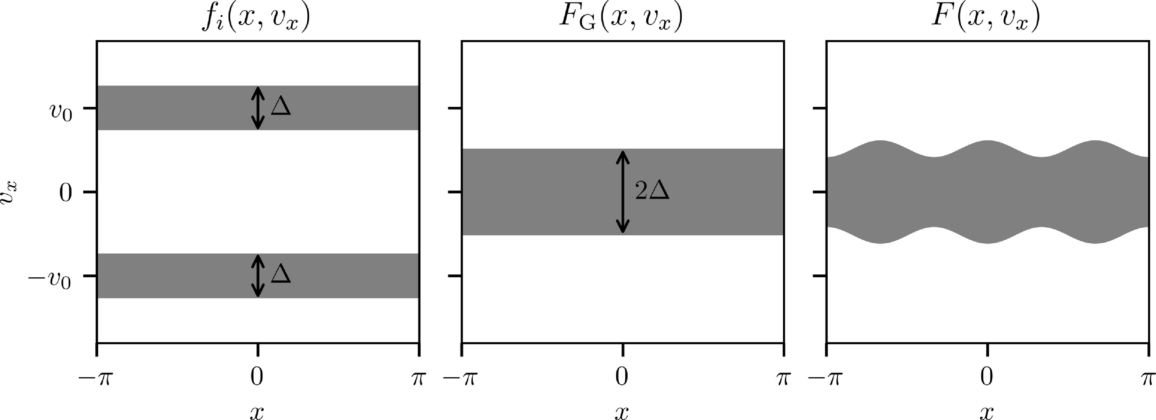
 FG
FG F
F
 Aph=λD,bg=k0=1
 n′′(π)<0
 t=0ωpe−1
 t=400ωpe−1
 ∼80%
∼80% λD
λD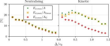
 AG
AG Alinear
 B=0
B=0 λD,bgk0=λD,bgkmin
 A
A
 t=0
t=0 Δ/v0=1.4
 Δ/v0=0.1
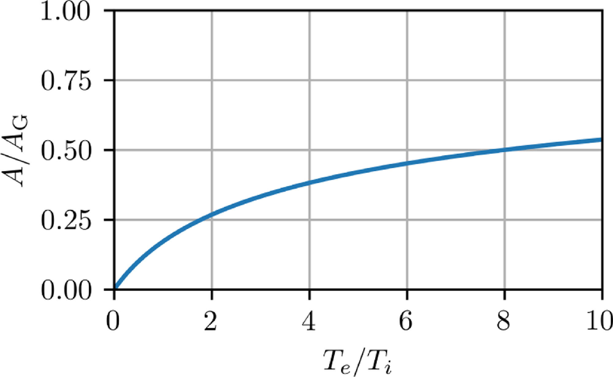
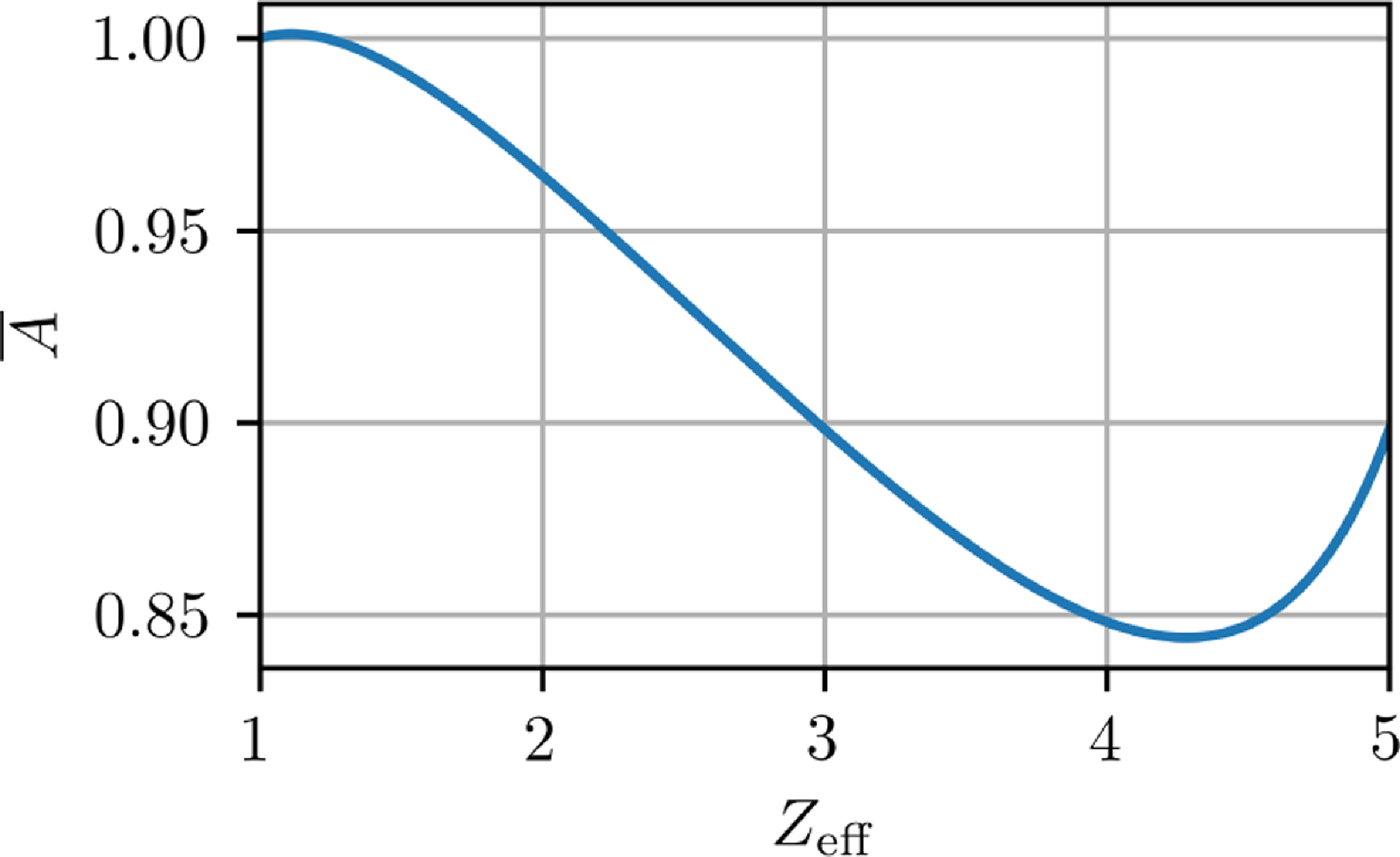
 Zeff
Zeff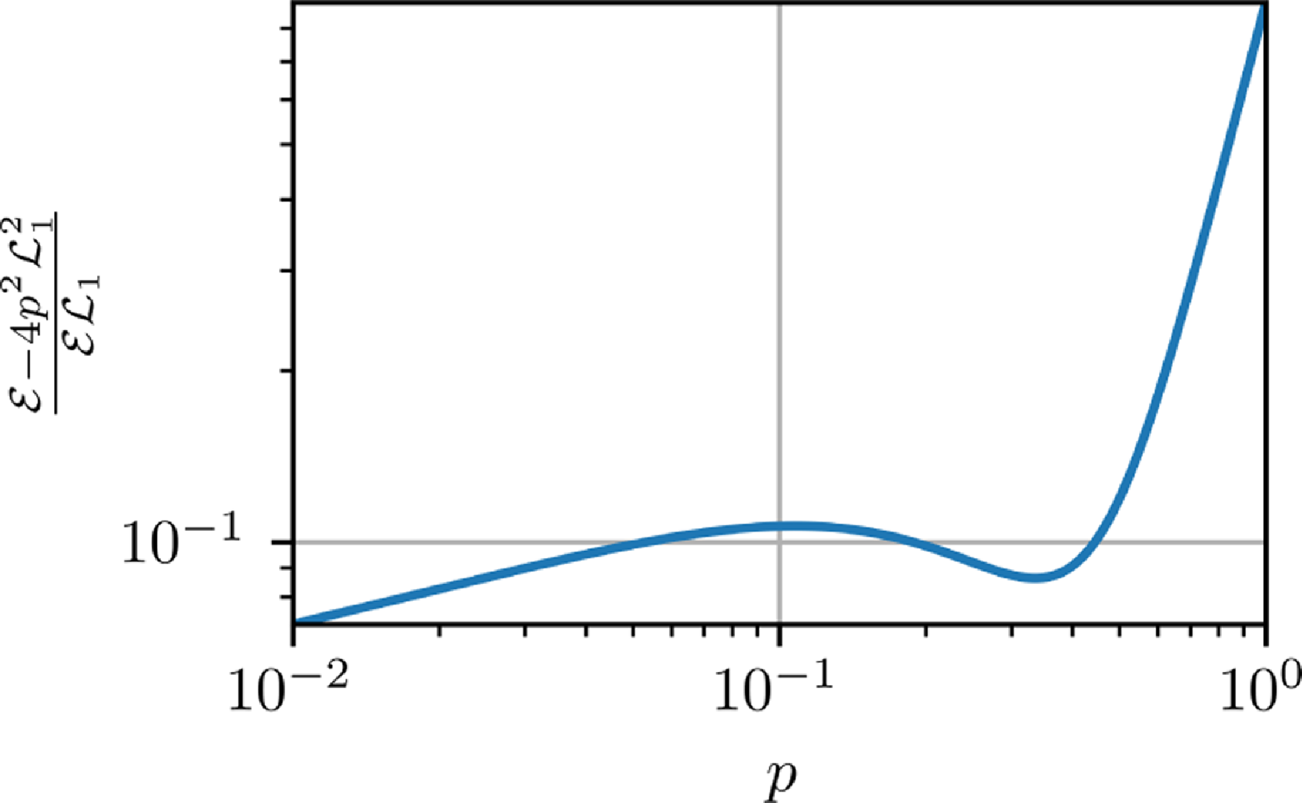
 p=vc,0/vα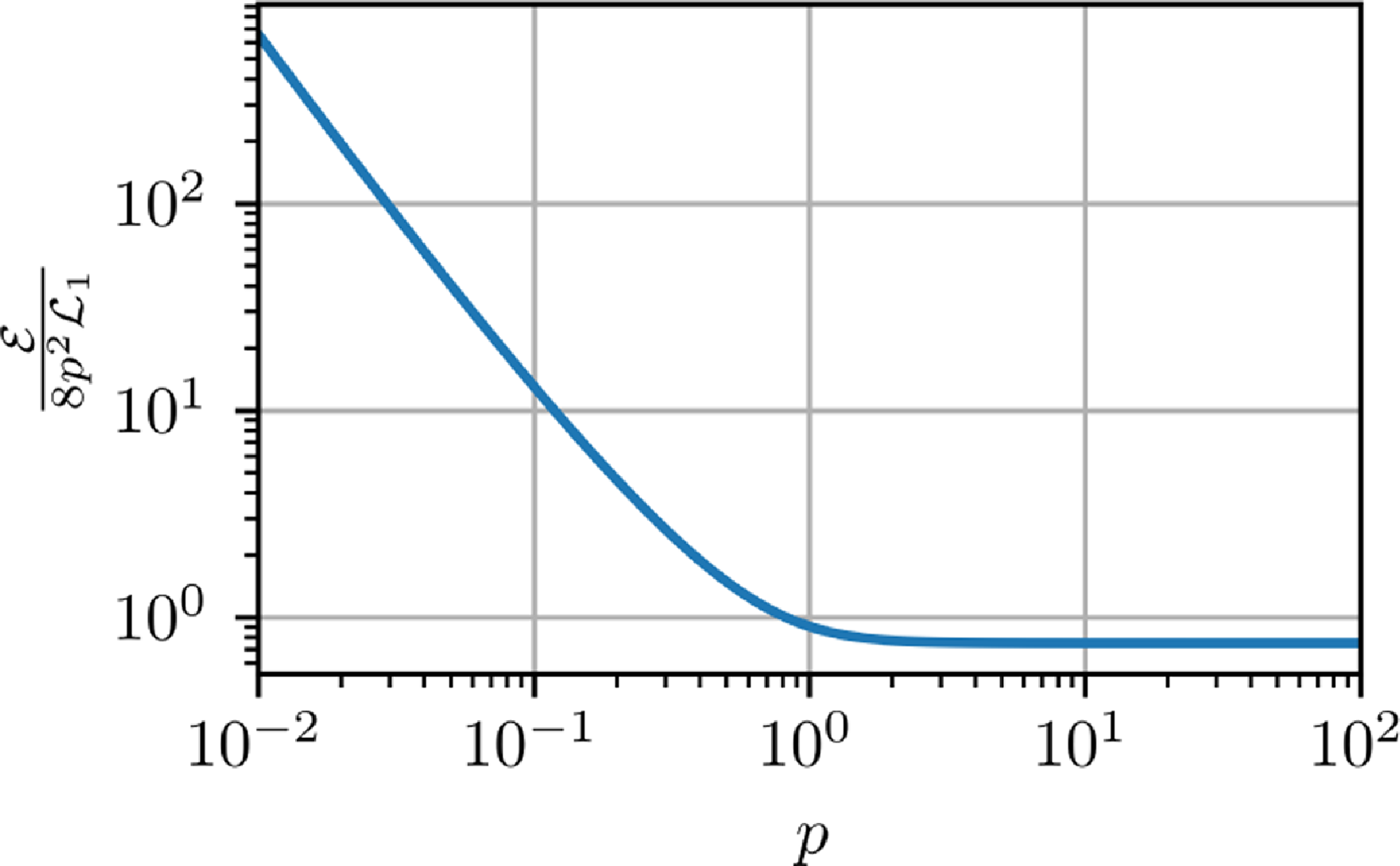
 E/8p2L1
 p=vc,0/vα
 c
c |c|
|c|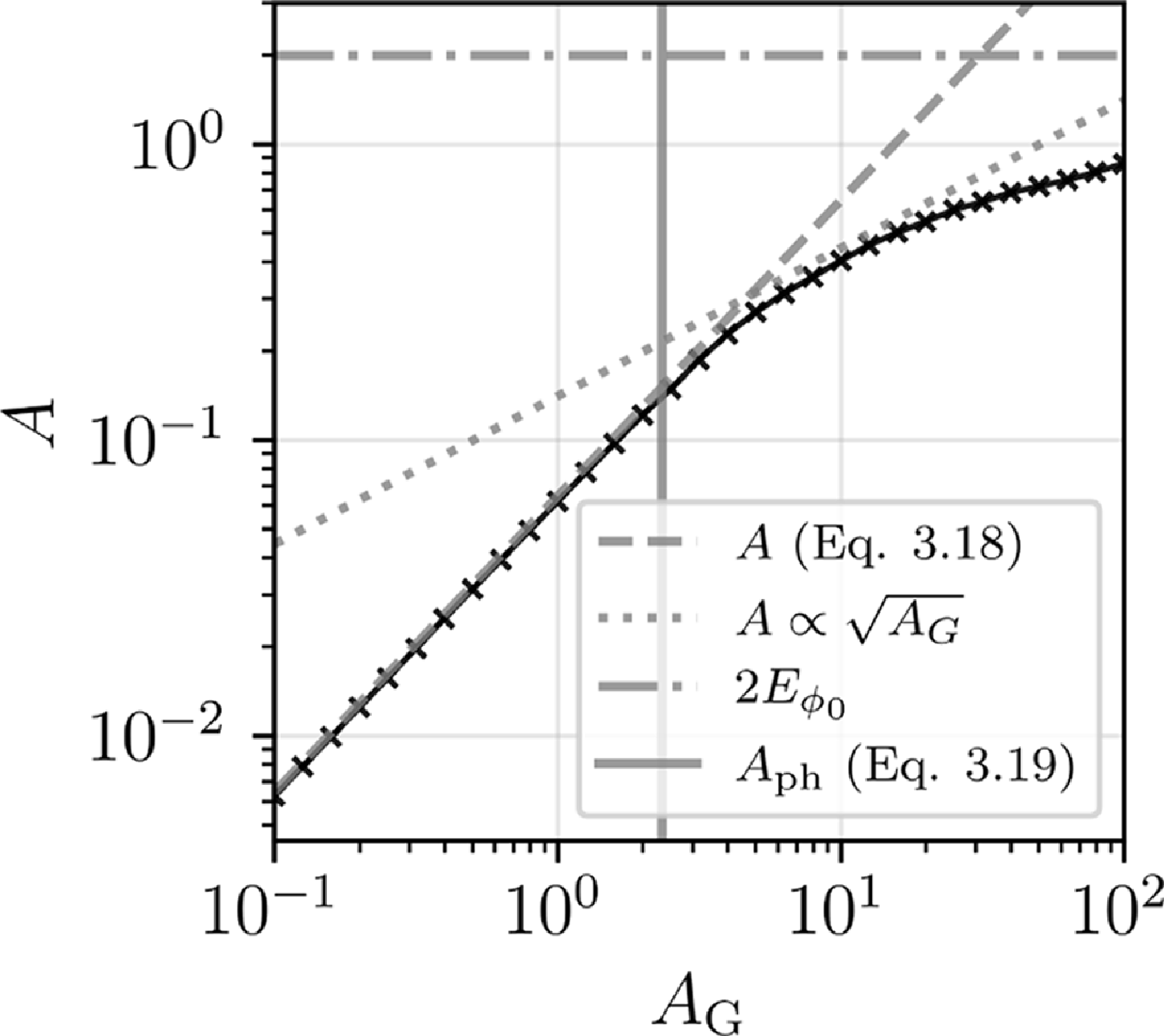
 AG
AG λD,bg=EG=Eϕ,0=Ebg=1
 x∈[0,6π)
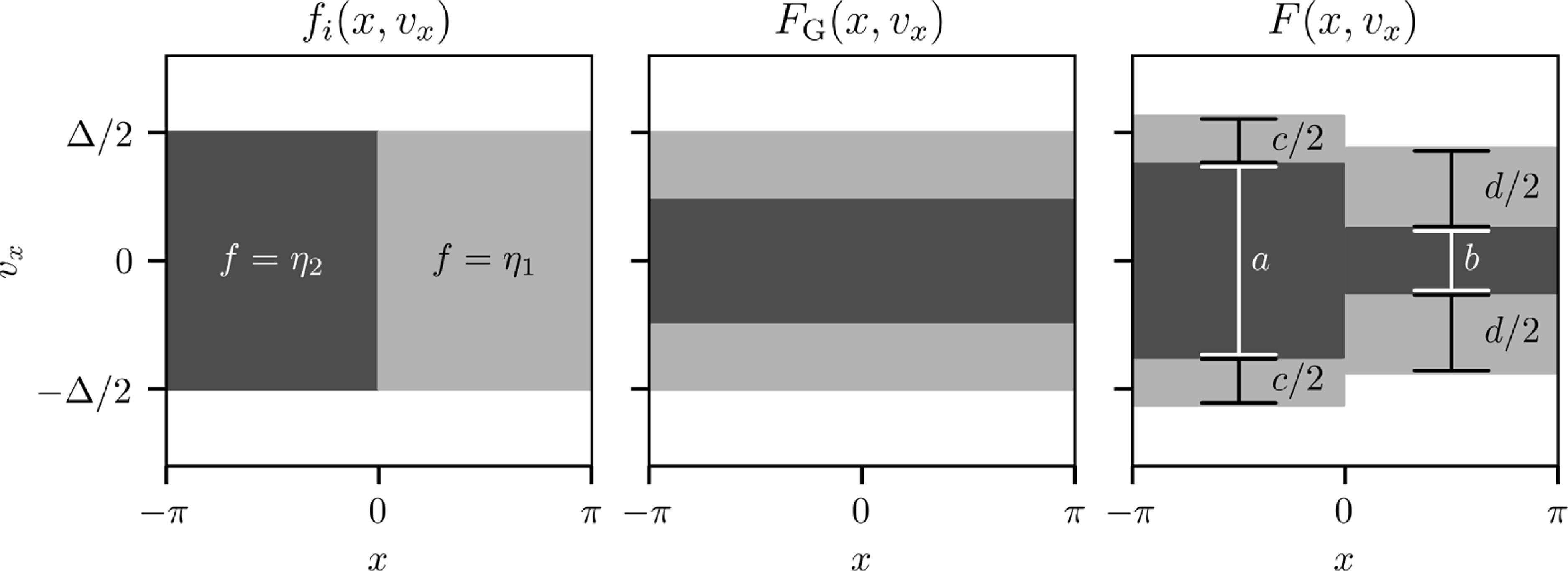

 δ
δ δ=1/3
δ=1/3 1−EG/Etot=1/12
 Open access

