


1. Introduction
Transverse injection of a liquid fuel stream into supersonic cross-flow is a convenient method of delivering fuel into a combustor, in particular for liquid fuel-based supersonic combustion ramjet (SCRAMJET) combustors, where the sudden exposure of the liquid jet to the cross-flow is mainly responsible for the liquid atomisation (Karagozian Reference Karagozian2010). During the combustion process, the air enters the combustor at supersonic speeds; hence, the residence time of the air inside the combustor is extremely short, necessitating rapid atomisation, dispersion and, subsequently, evaporation of liquid fuel (Fdida et al. Reference Fdida, Mallart-Martinez, Le Pichon and Vincent-Randonnier2022). The evolution of the jet and its interaction with the cross-flow is governed primarily by the momentum flux ratio of the injected jet to cross-flow (
 $J$
), although secondary features can also be important, e.g. free stream boundary-layer thickness. There is a wealth of knowledge available in the case of a transverse jet (either gas or liquid) into a subsonic cross-flow (Fric & Roshko Reference Fric and Roshko1994; Broumand & Birouk Reference Broumand and Birouk2016b
). However, the literature on experimental studies of a jet in supersonic cross-flow is limited, as emphasised by Mahesh (Reference Mahesh2013) in his review article. ‘Quantitative data at high speeds are less common, and visualisations still form an important component in estimating penetration and mixing’. Further, experimental investigation of the effect of orifice aspect ratio (AR) in relation to the atomisation of a liquid jet in supersonic cross-flow remains unexplored. The present study focuses on the detailed investigation of the influence of orifice AR on mean as well as unsteady flow field characteristics such as formation of surface waves on the liquid–gas interface, penetration height, shock structures and droplet dispersion in the spray plume. We shall see that the orifice AR significantly impacts the aforementioned flow field characteristics.
$J$
), although secondary features can also be important, e.g. free stream boundary-layer thickness. There is a wealth of knowledge available in the case of a transverse jet (either gas or liquid) into a subsonic cross-flow (Fric & Roshko Reference Fric and Roshko1994; Broumand & Birouk Reference Broumand and Birouk2016b
). However, the literature on experimental studies of a jet in supersonic cross-flow is limited, as emphasised by Mahesh (Reference Mahesh2013) in his review article. ‘Quantitative data at high speeds are less common, and visualisations still form an important component in estimating penetration and mixing’. Further, experimental investigation of the effect of orifice aspect ratio (AR) in relation to the atomisation of a liquid jet in supersonic cross-flow remains unexplored. The present study focuses on the detailed investigation of the influence of orifice AR on mean as well as unsteady flow field characteristics such as formation of surface waves on the liquid–gas interface, penetration height, shock structures and droplet dispersion in the spray plume. We shall see that the orifice AR significantly impacts the aforementioned flow field characteristics.
When a liquid jet is injected into a cross-flow, the forces (both pressure and shear forces) encountered by the liquid jet result in deformation and deflection of the injected jet in the direction of cross-flow. This also results in the atomisation of the liquid jet. The jet penetration trajectory and the atomisation characteristics of the injected liquid jet are key aspects in the design of the combustor. There are numerous studies available on injection into a subsonic cross-flow, in which various parameters are varied, e.g.
 $J$
(Wu et al. Reference Wu, Kirkendall, Fuller and Nejad1997, Reference Wu, Kirkendall, Fuller and Nejad1998), cross-flow Weber number (Sallam, Aalburg & Faeth Reference Sallam, Aalburg and Faeth2004), Reynolds number of the jet (Broumand & Birouk Reference Broumand and Birouk2017; Prakash et al. Reference Prakash, Sinha, Tomar and Ravikrishna2018), cross-flow turbulence (Broumand & Birouk Reference Broumand and Birouk2019), orifice
$J$
(Wu et al. Reference Wu, Kirkendall, Fuller and Nejad1997, Reference Wu, Kirkendall, Fuller and Nejad1998), cross-flow Weber number (Sallam, Aalburg & Faeth Reference Sallam, Aalburg and Faeth2004), Reynolds number of the jet (Broumand & Birouk Reference Broumand and Birouk2017; Prakash et al. Reference Prakash, Sinha, Tomar and Ravikrishna2018), cross-flow turbulence (Broumand & Birouk Reference Broumand and Birouk2019), orifice
 $\textit{AR}$
(Jadidi, Sreekumar & Dolatabadi Reference Jadidi, Sreekumar and Dolatabadi2019) as well as the properties of the jet (Sinha et al. Reference Sinha, Prakash, Mohan and Ravikrishna2015). From these studies, a wide variety of empirical correlations for the jet trajectory is available. For a given
$\textit{AR}$
(Jadidi, Sreekumar & Dolatabadi Reference Jadidi, Sreekumar and Dolatabadi2019) as well as the properties of the jet (Sinha et al. Reference Sinha, Prakash, Mohan and Ravikrishna2015). From these studies, a wide variety of empirical correlations for the jet trajectory is available. For a given
 $J$
and at a very low cross-flow Weber number (We
$J$
and at a very low cross-flow Weber number (We
 $_\infty =\rho _\infty U_\infty ^2 D / \sigma \lt$
10), the liquid column is free from large deformations. Its eventual breakup into ligaments and droplets is therefore due to inherent instabilities of the liquid jet (Sallam et al. Reference Sallam, Aalburg and Faeth2004). As the Weber number (We
$_\infty =\rho _\infty U_\infty ^2 D / \sigma \lt$
10), the liquid column is free from large deformations. Its eventual breakup into ligaments and droplets is therefore due to inherent instabilities of the liquid jet (Sallam et al. Reference Sallam, Aalburg and Faeth2004). As the Weber number (We
 $_\infty$
) increases (10–100), surface waves are formed on the windward side of the liquid column due to the Rayleigh–Taylor (Herrmann, Arienti & Soteriou Reference Herrmann, Arienti and Soteriou2011) or the Kelvin–Helmholtz (Arienti & Soteriou Reference Arienti and Soteriou2009) instabilities, or a combination of both. Furthermore, it is observed that the liquid column undergoes an increased deformation and a decrease in surface wavelength (
$_\infty$
) increases (10–100), surface waves are formed on the windward side of the liquid column due to the Rayleigh–Taylor (Herrmann, Arienti & Soteriou Reference Herrmann, Arienti and Soteriou2011) or the Kelvin–Helmholtz (Arienti & Soteriou Reference Arienti and Soteriou2009) instabilities, or a combination of both. Furthermore, it is observed that the liquid column undergoes an increased deformation and a decrease in surface wavelength (
 $\lambda$
) along with the mass stripping from the column surface. This occurs due to the shearing action of the cross-flow fluid (Mazallon, Dai & Faeth Reference Mazallon, Dai and Faeth1999; Sallam et al. Reference Sallam, Aalburg and Faeth2004; Behzad, Ashgriz & Mashayek Reference Behzad, Ashgriz and Mashayek2015). These observations have led to a regime map, characterising the liquid jet breakup behaviour for different We
$\lambda$
) along with the mass stripping from the column surface. This occurs due to the shearing action of the cross-flow fluid (Mazallon, Dai & Faeth Reference Mazallon, Dai and Faeth1999; Sallam et al. Reference Sallam, Aalburg and Faeth2004; Behzad, Ashgriz & Mashayek Reference Behzad, Ashgriz and Mashayek2015). These observations have led to a regime map, characterising the liquid jet breakup behaviour for different We
 $_\infty$
. Such regime maps have also been extensively studied for breakup of a single liquid drop in a flow (Pilch & Erdman Reference Pilch and Erdman1987; Theofanous & Li Reference Theofanous and Li2008; Theofanous Reference Theofanous2011; Sharma et al. Reference Sharma, Singh, Rao, Kumar and Basu2021). To summarise, at higher subsonic cross-flow velocities, the droplet fragmentation from the liquid jet arises initially due to surface breakup later followed by column breakup (Wu et al. Reference Wu, Kirkendall, Fuller and Nejad1997; Sallam et al. Reference Sallam, Aalburg and Faeth2004; Behzad et al. Reference Behzad, Ashgriz and Karney2015, Reference Behzad, Ashgriz and Mashayek2016). This leads to non-uniform distributions of drop size and velocities across the spray plume (Inamura & Nagai Reference Inamura and Nagai1997; Wu et al. Reference Wu, Kirkendall, Fuller and Nejad1998).
$_\infty$
. Such regime maps have also been extensively studied for breakup of a single liquid drop in a flow (Pilch & Erdman Reference Pilch and Erdman1987; Theofanous & Li Reference Theofanous and Li2008; Theofanous Reference Theofanous2011; Sharma et al. Reference Sharma, Singh, Rao, Kumar and Basu2021). To summarise, at higher subsonic cross-flow velocities, the droplet fragmentation from the liquid jet arises initially due to surface breakup later followed by column breakup (Wu et al. Reference Wu, Kirkendall, Fuller and Nejad1997; Sallam et al. Reference Sallam, Aalburg and Faeth2004; Behzad et al. Reference Behzad, Ashgriz and Karney2015, Reference Behzad, Ashgriz and Mashayek2016). This leads to non-uniform distributions of drop size and velocities across the spray plume (Inamura & Nagai Reference Inamura and Nagai1997; Wu et al. Reference Wu, Kirkendall, Fuller and Nejad1998).
At higher cross-flow Weber number (
 $\gt$
2000), as in the present study, the liquid jet undergoes intense deformation and atomisation, as well as deflection into the cross-flow, all a result of the higher pressure and shear forces acting on the jet. A schematic representation of this flow field is depicted in figure 1. Compared with the subsonic case, now there exists a three-dimensional bow shock, which also leads to a separation of the on-coming turbulent boundary layer. This results in significant shock wave boundary layer interactions (SWBLIs), which ultimately lead to large pressure pulsations around the injected jet or even inside the jet itself. This introduces substantial unsteadiness to the jet penetration, shock position and downstream spray characteristics (Medipati et al. Reference Medipati, Deivandren and Govardhan2023). Similar unsteady flow field interactions due to SWBLI in high-speed flows were investigated in the past by numerous researchers for various flow configurations (Dolling Reference Dolling2000; Ganapathisubramani, Clemens & Dolling Reference Ganapathisubramani, Clemens and Dolling2007; Dussauge & Piponniau Reference Dussauge and Piponniau2008; Mahesh Reference Mahesh2013; Clemens & Narayanaswamy Reference Clemens and Narayanaswamy2014; Murugan & Govardhan Reference Murugan and Govardhan2016; Munuswamy & Govardhan Reference Munuswamy and Govardhan2022). The key difference between the existing studies and the present study is that in earlier studies, the shock wave was formed because the obstruction was a solid body (Clemens & Narayanaswamy Reference Clemens and Narayanaswamy2014) or an injected sonic gaseous jet (Chai, Iyer & Mahesh Reference Chai, Iyer and Mahesh2015; Munuswamy & Govardhan Reference Munuswamy and Govardhan2022), whereas in the present study, it is due to the transverse injection of a (deformable) liquid jet. Although there exist considerable studies on a sonic jet in supersonic cross-flow (Mahesh Reference Mahesh2013), the focus of these studies was on mean and unsteady aspects of the flow field characteristics. Recently, by employing particle image velocimetry (PIV) both in the gaseous jet and on the cross-flow side, a detailed experimental investigation of these unsteady flow field interactions due to SWBLI was studied by Munuswamy & Govardhan (Reference Munuswamy and Govardhan2022). Their study revealed that high-speed boundary-layer streaks led to the downstream displacement of the separation shock as well as a reduction in jet penetration height, resulting in downstream motion of the bow shock. The opposite effects were seen for low-speed boundary-layer streaks. It is intuitive that similar unsteady interactions will occur upstream of a liquid jet when subjected to similar cross-flow conditions.
$\gt$
2000), as in the present study, the liquid jet undergoes intense deformation and atomisation, as well as deflection into the cross-flow, all a result of the higher pressure and shear forces acting on the jet. A schematic representation of this flow field is depicted in figure 1. Compared with the subsonic case, now there exists a three-dimensional bow shock, which also leads to a separation of the on-coming turbulent boundary layer. This results in significant shock wave boundary layer interactions (SWBLIs), which ultimately lead to large pressure pulsations around the injected jet or even inside the jet itself. This introduces substantial unsteadiness to the jet penetration, shock position and downstream spray characteristics (Medipati et al. Reference Medipati, Deivandren and Govardhan2023). Similar unsteady flow field interactions due to SWBLI in high-speed flows were investigated in the past by numerous researchers for various flow configurations (Dolling Reference Dolling2000; Ganapathisubramani, Clemens & Dolling Reference Ganapathisubramani, Clemens and Dolling2007; Dussauge & Piponniau Reference Dussauge and Piponniau2008; Mahesh Reference Mahesh2013; Clemens & Narayanaswamy Reference Clemens and Narayanaswamy2014; Murugan & Govardhan Reference Murugan and Govardhan2016; Munuswamy & Govardhan Reference Munuswamy and Govardhan2022). The key difference between the existing studies and the present study is that in earlier studies, the shock wave was formed because the obstruction was a solid body (Clemens & Narayanaswamy Reference Clemens and Narayanaswamy2014) or an injected sonic gaseous jet (Chai, Iyer & Mahesh Reference Chai, Iyer and Mahesh2015; Munuswamy & Govardhan Reference Munuswamy and Govardhan2022), whereas in the present study, it is due to the transverse injection of a (deformable) liquid jet. Although there exist considerable studies on a sonic jet in supersonic cross-flow (Mahesh Reference Mahesh2013), the focus of these studies was on mean and unsteady aspects of the flow field characteristics. Recently, by employing particle image velocimetry (PIV) both in the gaseous jet and on the cross-flow side, a detailed experimental investigation of these unsteady flow field interactions due to SWBLI was studied by Munuswamy & Govardhan (Reference Munuswamy and Govardhan2022). Their study revealed that high-speed boundary-layer streaks led to the downstream displacement of the separation shock as well as a reduction in jet penetration height, resulting in downstream motion of the bow shock. The opposite effects were seen for low-speed boundary-layer streaks. It is intuitive that similar unsteady interactions will occur upstream of a liquid jet when subjected to similar cross-flow conditions.
Schematic illustrating the main flow features in liquid jet injection into a supersonic cross-flow (Medipati, Deivandren & Govardhan Reference Medipati, Deivandren and Govardhan2023).

A large number of studies quantify the mean penetration height and suggest empirical correlations with the momentum flux ratio (
 $J$
) at different free stream Mach numbers (
$J$
) at different free stream Mach numbers (
 $M_\infty$
), primarily for circular liquid jet orifices (Lin et al. Reference Lin, Kennedy and Jackson2002, Reference Lin, Kennedy and Jackson2004; Beloki Perurena et al. Reference Beloki Perurena, Asma, Theunissen and Chazot2009; Ghenai, Sapmaz & Lin Reference Ghenai, Sapmaz and Lin2009; Sathiyamoorthy et al. Reference Sathiyamoorthy, Danish, Iyengar, Srinivas, Harikrishna, Muruganandam and Chakravarthy2020; Fdida et al. Reference Fdida, Mallart-Martinez, Le Pichon and Vincent-Randonnier2022; Medipati et al. Reference Medipati, Deivandren and Govardhan2023). In these studies,
$M_\infty$
), primarily for circular liquid jet orifices (Lin et al. Reference Lin, Kennedy and Jackson2002, Reference Lin, Kennedy and Jackson2004; Beloki Perurena et al. Reference Beloki Perurena, Asma, Theunissen and Chazot2009; Ghenai, Sapmaz & Lin Reference Ghenai, Sapmaz and Lin2009; Sathiyamoorthy et al. Reference Sathiyamoorthy, Danish, Iyengar, Srinivas, Harikrishna, Muruganandam and Chakravarthy2020; Fdida et al. Reference Fdida, Mallart-Martinez, Le Pichon and Vincent-Randonnier2022; Medipati et al. Reference Medipati, Deivandren and Govardhan2023). In these studies,
 $M_\infty$
(We
$M_\infty$
(We
 $_\infty$
) varies between 1.5 (Ghenai et al. Reference Ghenai, Sapmaz and Lin2009) and 6 (Beloki Perurena et al. Reference Beloki Perurena, Asma, Theunissen and Chazot2009), and comparison between these studies yields significant disparities in jet penetration height even at a fixed
$_\infty$
) varies between 1.5 (Ghenai et al. Reference Ghenai, Sapmaz and Lin2009) and 6 (Beloki Perurena et al. Reference Beloki Perurena, Asma, Theunissen and Chazot2009), and comparison between these studies yields significant disparities in jet penetration height even at a fixed
 $J$
(Medipati et al. Reference Medipati, Deivandren and Govardhan2023).
$J$
(Medipati et al. Reference Medipati, Deivandren and Govardhan2023).
The downstream spray characteristics for a circular liquid jet have been quantified (Lin, Kennedy & Jackson Reference Lin, Kennedy and Jackson2004; Medipati et al. Reference Medipati, Deivandren and Govardhan2023). Typically, the Sauter mean diameter (SMD) follows an ‘S’ shaped profile across the spray plume, with a mean droplet size of
 $O$
(10)
$O$
(10)
 $\unicode{x03BC} \mathrm{m}$
(Nejad & Schetz Reference Nejad and Schetz1983). The experimental quantitative trends are in close agreement with the numerically simulated results by Liu, Guo & Lin (Reference Liu, Guo and Lin2016) and Li et al. (Reference Li, Wang, Sun and Wang2017). The studies by Wu et al. (Reference Wu, Wang, Li and Zhang2015) showed a deviation in SMD profile from the existing ‘S’-shape when a kerosene jet is injected into a supersonic cross-flow; whereas the mean streamwise droplet velocity (
$\unicode{x03BC} \mathrm{m}$
(Nejad & Schetz Reference Nejad and Schetz1983). The experimental quantitative trends are in close agreement with the numerically simulated results by Liu, Guo & Lin (Reference Liu, Guo and Lin2016) and Li et al. (Reference Li, Wang, Sun and Wang2017). The studies by Wu et al. (Reference Wu, Wang, Li and Zhang2015) showed a deviation in SMD profile from the existing ‘S’-shape when a kerosene jet is injected into a supersonic cross-flow; whereas the mean streamwise droplet velocity (
 $U$
) variation across the plume follows a ‘C’-shaped profile (Medipati et al. Reference Medipati, Deivandren and Govardhan2023), which was also observed recently by Johnson et al. (Reference Johnson, Marsh, Douglas, Ochs, Hammack, Menon and Mazumdar2024) using digital in-line holography.
$U$
) variation across the plume follows a ‘C’-shaped profile (Medipati et al. Reference Medipati, Deivandren and Govardhan2023), which was also observed recently by Johnson et al. (Reference Johnson, Marsh, Douglas, Ochs, Hammack, Menon and Mazumdar2024) using digital in-line holography.
Employing non-circular jet orifices can act as a passive control strategy to manipulate the vortical structures present in the flow (Gutmark & Grinstein Reference Gutmark and Grinstein1999). Jets from elliptical orifices are more prone to breakup and result in smaller breakup lengths (Kasyap, Sivakumar & Raghunandan Reference Kasyap, Sivakumar and Raghunandan2009; Yu et al. Reference Yu, Yin, Deng, Jia, Ye, Xu and Xu2018, Reference Yu, Yin, Deng, Jia, Ye, Xu and Xu2019) when injected into a quiescent atmosphere. The presence of an extra instability (axis-switching phenomenon) in the case of elliptical jets leads to this earlier breakup. This was also seen as an increase in growth rate by Amini et al. (Reference Amini, Lv, Dolatabadi and Ihme2014), by comparing their experimental measurements of surface wavelength for different ellipticity with the theoretical calculations from the linear stability analysis. The injection of a water jet into a water tunnel using elliptical and circular orifices resulted in substantial differences in their near-field vortical structures as well as the scaling of their penetration heights (New et al. Reference New, Lim and Luo2003, Reference New, Lim and Luo2004; Lim, New & Luo Reference Lim, New and Luo2006), with orifice
 $\textit{AR}$
being a key parameter (New, Lim & Luo Reference New, Lim and Luo2003). Also, the injection of a sonic gaseous jet into a supersonic cross-flow (same phase) using an elliptical orifice exhibited significant differences in jet penetration height, shock structures and evolution of gaseous jet plume (Gruber et al. Reference Gruber, Nejad, Chen and Dutton1996, Reference Gruber, Nejad, Chen and Dutton2000). In particular, with
$\textit{AR}$
being a key parameter (New, Lim & Luo Reference New, Lim and Luo2003). Also, the injection of a sonic gaseous jet into a supersonic cross-flow (same phase) using an elliptical orifice exhibited significant differences in jet penetration height, shock structures and evolution of gaseous jet plume (Gruber et al. Reference Gruber, Nejad, Chen and Dutton1996, Reference Gruber, Nejad, Chen and Dutton2000). In particular, with
 $\textit{AR}$
= 0.26, the jet penetrated 20 % less than a circular jet for the same
$\textit{AR}$
= 0.26, the jet penetrated 20 % less than a circular jet for the same
 $J$
. This is due to the higher surface pressure force experienced by the jet when injected through different orifice shapes. From the foregoing discussion, it is evident that there have been no reported measurements in the literature pertaining to the injection of a liquid jet from non-circular orifices into a supersonic cross-flow; therefore, this is the focus of the present work.
$J$
. This is due to the higher surface pressure force experienced by the jet when injected through different orifice shapes. From the foregoing discussion, it is evident that there have been no reported measurements in the literature pertaining to the injection of a liquid jet from non-circular orifices into a supersonic cross-flow; therefore, this is the focus of the present work.
From the available literature on elliptical jets, both into quiescent and cross-flows, it is well understood that the mixing performance, as well as atomisation (Rajesh et al. Reference Rajesh, Kulkarni, Vankeswaram, Sakthikumar and Deivandren2023) of the elliptical jet, can be significantly different from the circular jet case. This provides motivation to investigate the flow field physics when a liquid jet is transversely injected into a supersonic cross-flow from an elliptical orifice. Therefore, the novelty of the current study lies in the detailed measurements and analysis of distinguishing features between the flow field interactions with circular and non-circular (elliptical) orifices. The primary goal is to understand how the orifice
 $\textit{AR}$
influences the formation of near-field windward surface waves, the liquid jet penetration and breakup behaviour, the corresponding shock structures along with their unsteady aspects, and the final droplet size and distribution.
$\textit{AR}$
influences the formation of near-field windward surface waves, the liquid jet penetration and breakup behaviour, the corresponding shock structures along with their unsteady aspects, and the final droplet size and distribution.
The rest of the paper is organised as follows. In § 2, we present the experimental details of the study including details of the test facility and the experimental techniques used. This is followed in § 3 by a discussion of the effect of orifice
 $\textit{AR}$
on the initial breakup mechanisms of the liquid jet and the associated shock structures seen ahead of the injected liquid jet. The mean and unsteady aspects of the liquid jet penetration into the supersonic cross-flow and their variations with orifice
$\textit{AR}$
on the initial breakup mechanisms of the liquid jet and the associated shock structures seen ahead of the injected liquid jet. The mean and unsteady aspects of the liquid jet penetration into the supersonic cross-flow and their variations with orifice
 $\textit{AR}$
are then discussed in § 4. Measurements of the final drop sizes in the spray formed downstream of the injected liquid jet are then presented and discussed in § 5, followed by the summary and conclusions in § 6.
$\textit{AR}$
are then discussed in § 4. Measurements of the final drop sizes in the spray formed downstream of the injected liquid jet are then presented and discussed in § 5, followed by the summary and conclusions in § 6.
2. Experimental details
2.1. Experimental facility and operating conditions
Experiments were conducted in an open circuit blow-down wind tunnel at the Interdisciplinary Center for Energy Research, Indian Institute of Science, Bangalore. All of the experiments were performed with a free stream Mach number (
 $M_\infty$
) of 2.5. The test section has a cross-section of 15 cm x 15 cm with a length of 1 m. Transparent windows on both the side and top of the test section allowed for optical access. The streamwise, cross-stream and spanwise directions are denoted by
$M_\infty$
) of 2.5. The test section has a cross-section of 15 cm x 15 cm with a length of 1 m. Transparent windows on both the side and top of the test section allowed for optical access. The streamwise, cross-stream and spanwise directions are denoted by
 $x$
,
$x$
,
 $y$
and
$y$
and
 $z$
, respectively, with
$z$
, respectively, with
 $x$
being the direction of cross-stream air and
$x$
being the direction of cross-stream air and
 $y$
the direction of injection of the liquid jet. The liquid nozzle was flush mounted on the tunnel wall, at a streamwise location of 100 mm from the C-D nozzle exit. The free stream (cross-stream) velocity (
$y$
the direction of injection of the liquid jet. The liquid nozzle was flush mounted on the tunnel wall, at a streamwise location of 100 mm from the C-D nozzle exit. The free stream (cross-stream) velocity (
 $U_\infty$
) and the incoming boundary-layer thickness (
$U_\infty$
) and the incoming boundary-layer thickness (
 $\delta$
) measured at this injection location using PIV were 585 m s−1 and 8.85 mm, respectively. The turbulence level measured in the free stream was lower than 1.5 %
$\delta$
) measured at this injection location using PIV were 585 m s−1 and 8.85 mm, respectively. The turbulence level measured in the free stream was lower than 1.5 %
 $U_\infty$
(Munuswamy Reference Munuswamy2020). The schematic of the wind tunnel, liquid injection system and sharp-edged nozzle are depicted in figures 2(a) and 2(b), respectively.
$U_\infty$
(Munuswamy Reference Munuswamy2020). The schematic of the wind tunnel, liquid injection system and sharp-edged nozzle are depicted in figures 2(a) and 2(b), respectively.
(a) Schematic of supersonic wind tunnel with liquid injection facility. (b) Schematic of the sharp-edged injector.
 $L$
and
$L$
and
 $D$
represent the length of the injector and the equivalent diameter of the orifice, respectively. Blue coloured arrow denotes the direction of water flow inside the nozzle.
$D$
represent the length of the injector and the equivalent diameter of the orifice, respectively. Blue coloured arrow denotes the direction of water flow inside the nozzle.

An elliptical and a circular orifice with an equivalent diameter (
 $D$
) of 1.2 mm and a length-to-diameter ratio (
$D$
) of 1.2 mm and a length-to-diameter ratio (
 $L/D$
) of 2 were selected for the current study. Using the two orifice shapes, three configurations were investigated based on the orientation of the orifice axis with respect to the cross-flow, as listed in table 1. It is important to note that when the
$L/D$
) of 2 were selected for the current study. Using the two orifice shapes, three configurations were investigated based on the orientation of the orifice axis with respect to the cross-flow, as listed in table 1. It is important to note that when the
 $\textit{AR}$
is changed, the centre of the orifice (
$\textit{AR}$
is changed, the centre of the orifice (
 $O$
) is kept at the same streamwise location (100 mm). This ensures that the injected liquid jet experiences a similar boundary layer thickness for all
$O$
) is kept at the same streamwise location (100 mm). This ensures that the injected liquid jet experiences a similar boundary layer thickness for all
 $\textit{AR}$
. Furthermore, the orifice exit area remains constant for all three cases. The details of the orifice shape, dimensions and its
$\textit{AR}$
. Furthermore, the orifice exit area remains constant for all three cases. The details of the orifice shape, dimensions and its
 $\textit{AR}$
for all three configurations are listed in table 1.
$\textit{AR}$
for all three configurations are listed in table 1.
Jet orifice geometric details used in the present study. The arrows denote the cross-stream direction. The streamwise and spanwise dimensions of the elliptical orifice are denoted as
 $a$
and
$a$
and
 $b$
, respectively.
$b$
, respectively.

The key dimensionless groups characterising the flow include:
-
(i) free stream (cross-flow) Mach number,
 $M_\infty = U_\infty /\sqrt {\gamma R T_\infty }$
;
$M_\infty = U_\infty /\sqrt {\gamma R T_\infty }$
; -
(ii) momentum flux ratio, defined as the ratio of momentum flux of the jet to momentum flux of the cross-flow, expressed as
$J = (\rho _j U_j^2)/(\rho _\infty U_\infty ^2)$
; -
(iii) aerodynamic Weber number, defined as the ratio of aerodynamic force to surface tension force, expressed as We
$_\infty =(\rho _\infty U_\infty ^2 D)/\sigma$
; -
(iv) Reynolds number of the liquid jet expressed as Re
$_j=(\rho _j U_j D)/\mu _j$
; -
(v) Orifice aspect ratio (
$\textit{AR}$
),

where
 $\rho _j$
,
$\rho _j$
,
 $U_j$
and
$U_j$
and
 $\rho _\infty$
,
$\rho _\infty$
,
 $U_\infty$
denote the density and velocity of the liquid jet and the cross-stream (free stream) air, respectively. The mean velocity of the liquid jet is estimated from the volume flow rate and the orifice exit area. The surface tension of the air–water interface and the dynamic viscosity of water are represented by
$U_\infty$
denote the density and velocity of the liquid jet and the cross-stream (free stream) air, respectively. The mean velocity of the liquid jet is estimated from the volume flow rate and the orifice exit area. The surface tension of the air–water interface and the dynamic viscosity of water are represented by
 $\sigma$
and
$\sigma$
and
 $\mu _j$
, respectively. The static temperature of the air, specific heat ratio and gas constant are denoted by
$\mu _j$
, respectively. The static temperature of the air, specific heat ratio and gas constant are denoted by
 $T_\infty, \gamma$
and
$T_\infty, \gamma$
and
 $R$
, respectively. The values or range of values of experimental parameters in the present investigation are summarised in table 2.
$R$
, respectively. The values or range of values of experimental parameters in the present investigation are summarised in table 2.
Values of experimental parameters considered in the present study during jet injection.

2.2. Experimental methods
Schematic showing the main components and arrangements of pulsed laser shadowgraphy (PLS), particle/droplet image analysis (PDIA) and particle image velocimetry (PIV) used in the present work. Visualisation plane in these experiments is the mid-span plane (
 $z$
= 0), as indicated with a green thin coloured sheet. The laser head is connected to a diffuser in the case of PLS and PDIA, and to the sheet optics for PIV.
$z$
= 0), as indicated with a green thin coloured sheet. The laser head is connected to a diffuser in the case of PLS and PDIA, and to the sheet optics for PIV.

Atomisation of a liquid jet in a supersonic flow is a multiscale phenomenon that demands different imaging systems operated at different spatial and temporal resolutions (Fdida et al. Reference Fdida, Mallart-Martinez, Le Pichon and Vincent-Randonnier2022). Therefore, in the present investigation, we have employed different experimental techniques to visualise the flow field interactions. The pulsed laser shadowgraphy (PLS) technique is employed to identify the differences in spray morphology and the global breakup behaviour for different values of orifice
 $\textit{AR}$
. This technique comprises a fluorescent diffuser plate illuminated by a nanosecond pulsed laser (Litron 200 mJ pulse−1, 532 nm dual cavity Nd-YAG laser), a 4MP (2360 × 1776 pixels) microsecond exposure CCD camera (Imager SX) and a programmable timing unit (PTU), which acts as a synchroniser between the laser and the camera, as shown schematically in figure 3. Images are acquired near the jet exit, focusing on a narrow field of view of approximately 30 mm x 23 mm (25
$\textit{AR}$
. This technique comprises a fluorescent diffuser plate illuminated by a nanosecond pulsed laser (Litron 200 mJ pulse−1, 532 nm dual cavity Nd-YAG laser), a 4MP (2360 × 1776 pixels) microsecond exposure CCD camera (Imager SX) and a programmable timing unit (PTU), which acts as a synchroniser between the laser and the camera, as shown schematically in figure 3. Images are acquired near the jet exit, focusing on a narrow field of view of approximately 30 mm x 23 mm (25
 $D$
x 19
$D$
x 19
 $D$
) using a 105 mm Nikon lens at an acquisition rate that was limited to the low pulse rate of 15 Hz. Therefore, to reveal the temporal dynamics as well as the complex shock structures involved during the jet cross-flow interaction, high-speed shadowgraphy was employed, where the framing rate was 10 000 Hz. The major differences between the PLS and high-speed shadowgraphy are the light source, camera and acquisition rate. In this technique, instead of a diffused laser light source, a collimated light beam was produced using a spherical concave mirror (20 cm in diameter) and a halogen lamp (150 W). A high-speed camera (Photron, FASTCAM SA5) with a microsecond exposure setting was used to acquire the images. These images were acquired at 10 000 Hz with a pixel resolution of 30 pixels mm−1 using a 105 mm Nikon lens in front of the camera. This allows visualisation of a very narrow field of view of approximately 15
$D$
) using a 105 mm Nikon lens at an acquisition rate that was limited to the low pulse rate of 15 Hz. Therefore, to reveal the temporal dynamics as well as the complex shock structures involved during the jet cross-flow interaction, high-speed shadowgraphy was employed, where the framing rate was 10 000 Hz. The major differences between the PLS and high-speed shadowgraphy are the light source, camera and acquisition rate. In this technique, instead of a diffused laser light source, a collimated light beam was produced using a spherical concave mirror (20 cm in diameter) and a halogen lamp (150 W). A high-speed camera (Photron, FASTCAM SA5) with a microsecond exposure setting was used to acquire the images. These images were acquired at 10 000 Hz with a pixel resolution of 30 pixels mm−1 using a 105 mm Nikon lens in front of the camera. This allows visualisation of a very narrow field of view of approximately 15
 $D$
x 20
$D$
x 20
 $D$
in the streamwise and transverse directions, respectively. In both techniques, the spray was illuminated through transparent windows on the back side and the density gradients were captured by a camera viewing through the transparent front-side window.
$D$
in the streamwise and transverse directions, respectively. In both techniques, the spray was illuminated through transparent windows on the back side and the density gradients were captured by a camera viewing through the transparent front-side window.
The microscopic details of the downstream spray droplets, viz. droplet size and velocities, were determined by using particle/droplet image analysis (PDIA). This is a well-established technique and has been applied to a variety of two-phase flow scenarios, ranging from ambient sprays (Kashdan et al. Reference Kashdan, Shrimpton and Whybrew2003, Reference Kashdan, Shrimpton and Whybrew2004; Kourmatzis, Pham & Masri Reference Kourmatzis, Pham and Masri2015) to liquid jets in subsonic cross-flow (Sinha et al. Reference Sinha, Prakash, Mohan and Ravikrishna2015; Prakash et al. Reference Prakash, Sinha, Tomar and Ravikrishna2018). Recently, Medipati et al. (Reference Medipati, Deivandren and Govardhan2023) also used the technique for a transverse circular jet in a supersonic flow case and shown that the droplet size data across the plume are in good agreement with the well-established phase Doppler particle analyser (PDPA) measurements in a similar flow configuration (Lin et al. Reference Lin, Kennedy and Jackson2004). The experimental set-up is similar to PLS except that the lens connected to the camera head was replaced with a long-distance microscope (LDM) (Questar, QM-100). This helped visualise the flow down to a very small field of view of approximately 2 mm x 1.5 mm. The chosen laser pulse duration (4 ns), along with a microsecond exposure camera, enabled us to obtain high-resolution instantaneous spray images with negligible motion blur. By operating the laser in a double exposure mode with a known interframe time of 0.5
 $\unicode{x03BC}$
s, time delayed pairs of images were captured. Particle tracking velocimetry (PTV) was employed on these time delayed pairs of images to obtain the velocity achieved by the spray droplets. It may be noted that the recent droplet velocity measurements obtained by digital inline holography (Johnson et al. Reference Johnson, Marsh, Douglas, Ochs, Hammack, Menon and Mazumdar2024) for a similar circular jet in the supersonic cross-flow configuration were found to be in good agreement with the velocities obtained by particle tracking through PDIA measurements (Medipati et al. Reference Medipati, Deivandren and Govardhan2023). At each station in the spray plume, a large number of instantaneous images (approximately 500) were captured during a single run. This resulted in the collection of many droplets for the estimation of long time averaged statistics of droplet size and velocities. The process was repeated at various stations in the spray plume to determine the effect of
$\unicode{x03BC}$
s, time delayed pairs of images were captured. Particle tracking velocimetry (PTV) was employed on these time delayed pairs of images to obtain the velocity achieved by the spray droplets. It may be noted that the recent droplet velocity measurements obtained by digital inline holography (Johnson et al. Reference Johnson, Marsh, Douglas, Ochs, Hammack, Menon and Mazumdar2024) for a similar circular jet in the supersonic cross-flow configuration were found to be in good agreement with the velocities obtained by particle tracking through PDIA measurements (Medipati et al. Reference Medipati, Deivandren and Govardhan2023). At each station in the spray plume, a large number of instantaneous images (approximately 500) were captured during a single run. This resulted in the collection of many droplets for the estimation of long time averaged statistics of droplet size and velocities. The process was repeated at various stations in the spray plume to determine the effect of
 $\textit{AR}$
on the dispersion of droplets in the spray plume. It is important to note that this technique captures and quantifies the sizes as well as velocities of both spherical and non-spherical droplets (Kashdan et al. Reference Kashdan, Shrimpton and Whybrew2003, Reference Kashdan, Shrimpton and Whybrew2004). A concern with PDIA is that the technique has a limitation in resolving smaller droplet sizes below 4–5
$\textit{AR}$
on the dispersion of droplets in the spray plume. It is important to note that this technique captures and quantifies the sizes as well as velocities of both spherical and non-spherical droplets (Kashdan et al. Reference Kashdan, Shrimpton and Whybrew2003, Reference Kashdan, Shrimpton and Whybrew2004). A concern with PDIA is that the technique has a limitation in resolving smaller droplet sizes below 4–5
 $\unicode{x03BC}$
m, due to diffraction limits (Sinha et al. Reference Sinha, Prakash, Mohan and Ravikrishna2015; Prakash et al. Reference Prakash, Sinha, Tomar and Ravikrishna2018). Hence, in the present work, droplet sizes below 5
$\unicode{x03BC}$
m, due to diffraction limits (Sinha et al. Reference Sinha, Prakash, Mohan and Ravikrishna2015; Prakash et al. Reference Prakash, Sinha, Tomar and Ravikrishna2018). Hence, in the present work, droplet sizes below 5
 $\unicode{x03BC}$
m are not considered and are not used for the calculation of drop size statistics. Its effect on the values of SMD is minimal as the SMD mean is closer to larger droplets in the distribution. The uncertainty in drop size measurement with this technique, as calculated using the procedure of Sinha et al. (Reference Sinha, Prakash, Mohan and Ravikrishna2015), was found to be below 2
$\unicode{x03BC}$
m are not considered and are not used for the calculation of drop size statistics. Its effect on the values of SMD is minimal as the SMD mean is closer to larger droplets in the distribution. The uncertainty in drop size measurement with this technique, as calculated using the procedure of Sinha et al. (Reference Sinha, Prakash, Mohan and Ravikrishna2015), was found to be below 2
 $\unicode{x03BC}$
m.
$\unicode{x03BC}$
m.
To understand the source of unsteadiness in jet penetration height and shock motion, PIV was used upstream of the jet exit. The experimental test set-up for PIV remained the same as PLS and PDIA, but with minor changes on the laser side. The fluorescent diffuser plate connected to the laser head during PLS and PDIA was replaced with a 1.5 mm thick laser sheet with sheet optics (
 $f$
= −10 mm). The laser sheet was allowed to enter the test section transversely through the transparent top window (spanwise central plane,
$f$
= −10 mm). The laser sheet was allowed to enter the test section transversely through the transparent top window (spanwise central plane,
 $z = 0$
) to illuminate the plane normal to the bottom wall (
$z = 0$
) to illuminate the plane normal to the bottom wall (
 $x$
–
$x$
–
 $y$
). The camera (Imager SX), equipped with a Nikon 105 mm f/2.8D lens along with a 532 nm bandpass filter, was used for viewing the flow through the transparent side window. These experiments were performed during liquid jet injection with a field of view of approximately 25
$y$
). The camera (Imager SX), equipped with a Nikon 105 mm f/2.8D lens along with a 532 nm bandpass filter, was used for viewing the flow through the transparent side window. These experiments were performed during liquid jet injection with a field of view of approximately 25
 $D$
x 15
$D$
x 15
 $D$
. In this case, the free stream air was seeded with olive oil particles of 1
$D$
. In this case, the free stream air was seeded with olive oil particles of 1
 $\unicode{x03BC}$
m size, which acted as tracer particles and was introduced into the flow upstream of the settling chamber. To reduce the reflections from solid surfaces for the near-wall PIV measurements, a fluorescent paint was prepared, which contained a mixture of 3 g rhodamine 6G (C28H31N2O3Cl), 10 mL ethanol and 500 mL transparent acrylic paint (water soluble), and was coated on the wall surfaces. The images were acquired in a double exposure mode with an interframe time of 0.5
$\unicode{x03BC}$
m size, which acted as tracer particles and was introduced into the flow upstream of the settling chamber. To reduce the reflections from solid surfaces for the near-wall PIV measurements, a fluorescent paint was prepared, which contained a mixture of 3 g rhodamine 6G (C28H31N2O3Cl), 10 mL ethanol and 500 mL transparent acrylic paint (water soluble), and was coated on the wall surfaces. The images were acquired in a double exposure mode with an interframe time of 0.5
 $\unicode{x03BC}$
s similar to PDIA. These instantaneous images were processed using Davis 8.4.0 software (LaVision GmbH) by adaptive correlation with multiple passes to obtain the PIV velocity fields. The final window size used was 32 x 16 pixels with 75 % overlap. The low/high momentum streaks present inside the boundary layer extend up to 40
$\unicode{x03BC}$
s similar to PDIA. These instantaneous images were processed using Davis 8.4.0 software (LaVision GmbH) by adaptive correlation with multiple passes to obtain the PIV velocity fields. The final window size used was 32 x 16 pixels with 75 % overlap. The low/high momentum streaks present inside the boundary layer extend up to 40
 $\delta$
in streamwise and 0.5
$\delta$
in streamwise and 0.5
 $\delta$
in spanwise directions (Ganapathisubramani et al. Reference Ganapathisubramani, Clemens and Dolling2007), which implies that we have an adequately large number of vectors (approximately 18) in the streamwise direction. Detailed information about the PIV used in the present study can be found in our previous studies (Murugan & Govardhan Reference Murugan and Govardhan2016; Munuswamy & Govardhan Reference Munuswamy and Govardhan2022). It is important to note that in the present investigation, all the measurements were carried out on the mid-spanwise plane (
$\delta$
in spanwise directions (Ganapathisubramani et al. Reference Ganapathisubramani, Clemens and Dolling2007), which implies that we have an adequately large number of vectors (approximately 18) in the streamwise direction. Detailed information about the PIV used in the present study can be found in our previous studies (Murugan & Govardhan Reference Murugan and Govardhan2016; Munuswamy & Govardhan Reference Munuswamy and Govardhan2022). It is important to note that in the present investigation, all the measurements were carried out on the mid-spanwise plane (
 $z$
= 0), as indicated by the green colour plane in figure 3.
$z$
= 0), as indicated by the green colour plane in figure 3.
3. Breakup mechanism and shock structures
In this section, we begin by presenting the influence of orifice AR on the observed formation of windward surface waves and discuss the associated initial breakup mechanisms of the liquid jet. This is followed by a discussion on the shock structures found ahead of the liquid jet and the variations seen in these shocks for different orifice AR.
3.1. Initial breakup mechanism of liquid jet
High-resolution instantaneous visualisations of the water jet in the supersonic cross-flow of
 $M_\infty$
= 2.5, captured using pulsed laser shadowgraphy highlighting the differences in the evolution of the surface waves in the windward side of the jet. These are acquired for (a)
$M_\infty$
= 2.5, captured using pulsed laser shadowgraphy highlighting the differences in the evolution of the surface waves in the windward side of the jet. These are acquired for (a)
 $\textit{AR}$
= 0.3, (b)
$\textit{AR}$
= 0.3, (b)
 $\textit{AR}$
= 1 and (c)
$\textit{AR}$
= 1 and (c)
 $\textit{AR}$
= 3.3, and
$\textit{AR}$
= 3.3, and
 $ J$
= 3.7. Zoomed-in visualisations near the jet exit on the windward side are shown as insets on the left side.
$ J$
= 3.7. Zoomed-in visualisations near the jet exit on the windward side are shown as insets on the left side.
 $\lambda$
and
$\lambda$
and
 $\delta$
represent the surface wavelength and mean boundary-layer thickness, respectively. The column breakup location is indicated with a red coloured dot, and its instantaneous positions from the orifice centre in the streamwise and transverse directions are
$\delta$
represent the surface wavelength and mean boundary-layer thickness, respectively. The column breakup location is indicated with a red coloured dot, and its instantaneous positions from the orifice centre in the streamwise and transverse directions are
 $x_{b}$
and
$x_{b}$
and
 $y_{b}$
, respectively.
$y_{b}$
, respectively.

Short-exposure (18
 $\unicode{x03BC}$
s) visualisations of the injected water jet into the supersonic cross-flow acquired using pulsed laser shadowgraphy are shown in figure 4. A large set of such instantaneous images revealed a significant influence of
$\unicode{x03BC}$
s) visualisations of the injected water jet into the supersonic cross-flow acquired using pulsed laser shadowgraphy are shown in figure 4. A large set of such instantaneous images revealed a significant influence of
 $\textit{AR}$
on the formation of surface waves on the windward side of the liquid jet. In each
$\textit{AR}$
on the formation of surface waves on the windward side of the liquid jet. In each
 $\textit{AR}$
case, as the jet traverses into the supersonic cross-flow, it is observed that near the jet exit (windward side), the injected jet is relatively free from surface deformations, presumably because of the wall boundary layer. A little further into the cross-flow, surface waves are seen on the windward side, as expected (Sallam et al. Reference Sallam, Aalburg and Faeth2004). These are likely due to the large accelerations experienced by the injected liquid jet when suddenly exposed to high-speed air (lighter) cross-flow. This accelerative destabilisation mechanism is the well-known Rayleigh–Taylor instability (RTI), which occurs when a low-density fluid accelerates over a high-density fluid (Taylor Reference Taylor1950). For
$\textit{AR}$
case, as the jet traverses into the supersonic cross-flow, it is observed that near the jet exit (windward side), the injected jet is relatively free from surface deformations, presumably because of the wall boundary layer. A little further into the cross-flow, surface waves are seen on the windward side, as expected (Sallam et al. Reference Sallam, Aalburg and Faeth2004). These are likely due to the large accelerations experienced by the injected liquid jet when suddenly exposed to high-speed air (lighter) cross-flow. This accelerative destabilisation mechanism is the well-known Rayleigh–Taylor instability (RTI), which occurs when a low-density fluid accelerates over a high-density fluid (Taylor Reference Taylor1950). For
 $\textit{AR}$
= 0.3 (figure 4
a), it is evident that the surface waves formed have a larger wavelength (
$\textit{AR}$
= 0.3 (figure 4
a), it is evident that the surface waves formed have a larger wavelength (
 $\lambda)$
when compared with those for
$\lambda)$
when compared with those for
 $\textit{AR}$
= 1 (figure 4
b), with the liquid column deformations in both these cases being relatively smooth. In contrast, the AR = 3.3 case (figure 4
c) has a much smaller windward surface wavelength and the liquid column deformations are not as smooth as the previous cases. These differences seen in the observed surface waves between the different
$\textit{AR}$
= 1 (figure 4
b), with the liquid column deformations in both these cases being relatively smooth. In contrast, the AR = 3.3 case (figure 4
c) has a much smaller windward surface wavelength and the liquid column deformations are not as smooth as the previous cases. These differences seen in the observed surface waves between the different
 $\textit{AR}$
cases studied is indicative of significant variations in the primary destabilisation mechanism with orifice AR, as discussed now.
$\textit{AR}$
cases studied is indicative of significant variations in the primary destabilisation mechanism with orifice AR, as discussed now.
The primary instability mechanism of the liquid jet in the present experiments shares common features with other well-studied, two-phase flow scenarios, namely, atomisation of a droplet in high-speed cross-flow (Joseph, Belanger & Beavers Reference Joseph, Belanger and Beavers1999) and atomisation of a liquid jet when injected parallel to the high-speed gas stream (Varga, Lasheras & Hopfinger Reference Varga, Lasheras and Hopfinger2003; Maarmottant & Villermaux Reference Maarmottant and Villermaux2004). When a liquid drop is placed in a supersonic flow along with the initial flattening of the droplet perpendicular to the air stream (pressure difference), surface waves are formed on the windward side of the drop surface due to the strong accelerations experienced by the liquid droplet perpendicular to the interface and directed from gas to liquid. Such a droplet–air interaction will make the droplet unstable due to the RTI. These surface waves are driven from the stagnation point towards the equator of the drop by the shear flow of the gas, which can in turn also lead to Kelvin–Helmholtz instability (KHI). Close to the stagnation region of the drop, it is the RTI that will be dominant, as the KHI is negligible due to the fact that the tangential velocity is close to zero in this region. When these RT waves around the stagnation region are sufficiently amplified, the droplet can undergo catastrophic breakup into finer droplets (Joseph et al. Reference Joseph, Belanger and Beavers1999). However, further away from the stagnation region, the shear is significant and the KHI can also be important.
Schematic showing the variation in jet and cross-flow interaction and atomisation mechanisms for different ARs and at different transverse heights. Panels (a,b,c), (d,e,f) and (g,h,i) represent the cross-section of the jet at the orifice exit, the deformed jet slice and the spray core in the transverse plane (x–z), respectively. The arrows in panels (a,b,c) indicate the free stream direction. The liquid surface participating in the shear breakup is highlighted with red colour.

A similar scenario may also be anticipated in the present study, where instead of the flattened drop, we consider the flattened/deformed liquid jet slice at a given height from the wall. This is illustrated schematically in figure 5 for each of the three different orifice
 $\textit{AR}$
cases studied here, with each row corresponding to a given
$\textit{AR}$
cases studied here, with each row corresponding to a given
 $\textit{AR}$
. In the figure, the first column (panels a,b,c) indicates the orifice geometry, the second column (panels d,e,f), the flattened or deformed liquid jet slice, and the third column (panels g,h,i), the associated flow field with spray. As seen from the schematics, there are considerable differences between the three
$\textit{AR}$
. In the figure, the first column (panels a,b,c) indicates the orifice geometry, the second column (panels d,e,f), the flattened or deformed liquid jet slice, and the third column (panels g,h,i), the associated flow field with spray. As seen from the schematics, there are considerable differences between the three
 $\textit{AR}$
cases, and this is discussed further now, starting from the circular orifice (
$\textit{AR}$
cases, and this is discussed further now, starting from the circular orifice (
 $\textit{AR}$
= 1) case, and moving onto the
$\textit{AR}$
= 1) case, and moving onto the
 $\textit{AR}=3.3$
and
$\textit{AR}=3.3$
and
 $\textit{AR}=0.3$
cases.
$\textit{AR}=0.3$
cases.
The jet slice in
 $\textit{AR}$
= 1 deforms in the lateral direction into a cupcake shape and flattens, which is attributed to the pressure difference between the windward (high pressure) and leeward (low pressure) sides of the jet slice (Joseph et al. Reference Joseph, Belanger and Beavers1999; Chai et al. Reference Chai, Iyer and Mahesh2015; Behzad, Ashgriz & Karney Reference Behzad, Ashgriz and Karney2016). Along with the strong acceleration of the liquid slice due to RTI, the cross-flow fluid accelerates around the low horizontal momentum jet resulting in high levels of shear on the lateral sides of the jet leading to KHI (Joseph et al. Reference Joseph, Belanger and Beavers1999; Chai et al. Reference Chai, Iyer and Mahesh2015), which results in liquid stripping from the jet slice (figure 5
e). As the liquid slice traverses further, the flattening of the liquid slice continues and the increased projected frontal area results in a significant rise in aerodynamic drag forces (Wu et al. Reference Wu, Kirkendall, Fuller and Nejad1997). This eventually disintegrates the bulk liquid mass into liquid clumps due to RTI, which has been referred to as column breakup (Wu et al. Reference Wu, Kirkendall, Fuller and Nejad1997) (see figure 4). Simultaneously, there is the formation of ligaments and droplets from the jet surface due to shear instability caused by the KH waves (Xiao et al. Reference Xiao, Wang, Sun, Liang and Liu2016). Together, they result in the formation of the spray plume core (figure 5
h). These liquid clumps, ligaments and droplets will further undergo fragmentation (secondary atomisation) to produce finer droplets because of the continuous interaction with the surrounding fluid.
$\textit{AR}$
= 1 deforms in the lateral direction into a cupcake shape and flattens, which is attributed to the pressure difference between the windward (high pressure) and leeward (low pressure) sides of the jet slice (Joseph et al. Reference Joseph, Belanger and Beavers1999; Chai et al. Reference Chai, Iyer and Mahesh2015; Behzad, Ashgriz & Karney Reference Behzad, Ashgriz and Karney2016). Along with the strong acceleration of the liquid slice due to RTI, the cross-flow fluid accelerates around the low horizontal momentum jet resulting in high levels of shear on the lateral sides of the jet leading to KHI (Joseph et al. Reference Joseph, Belanger and Beavers1999; Chai et al. Reference Chai, Iyer and Mahesh2015), which results in liquid stripping from the jet slice (figure 5
e). As the liquid slice traverses further, the flattening of the liquid slice continues and the increased projected frontal area results in a significant rise in aerodynamic drag forces (Wu et al. Reference Wu, Kirkendall, Fuller and Nejad1997). This eventually disintegrates the bulk liquid mass into liquid clumps due to RTI, which has been referred to as column breakup (Wu et al. Reference Wu, Kirkendall, Fuller and Nejad1997) (see figure 4). Simultaneously, there is the formation of ligaments and droplets from the jet surface due to shear instability caused by the KH waves (Xiao et al. Reference Xiao, Wang, Sun, Liang and Liu2016). Together, they result in the formation of the spray plume core (figure 5
h). These liquid clumps, ligaments and droplets will further undergo fragmentation (secondary atomisation) to produce finer droplets because of the continuous interaction with the surrounding fluid.
In the case of
 $\textit{AR}$
= 3.3 (figure 5
c), the cross-flow experiences the jet slice, which is an already deformed one in the lateral direction due to the orientation of the major axis perpendicular to the cross-flow. This results in a much stronger acceleration of the jet slice (amplified RTI) along with an enhanced flattening in the lateral direction (figure 5
f) compared with the
$\textit{AR}$
= 3.3 (figure 5
c), the cross-flow experiences the jet slice, which is an already deformed one in the lateral direction due to the orientation of the major axis perpendicular to the cross-flow. This results in a much stronger acceleration of the jet slice (amplified RTI) along with an enhanced flattening in the lateral direction (figure 5
f) compared with the
 $\textit{AR}$
= 1 case. Hence, the liquid jet can undergo catastrophic breakup with the formation of a fine spray mostly due to the amplified RTI. This results in greater liquid jet deflection, early formation of droplets and extended deformation of the liquid column. Hence, the bulk liquid mass undergoes intense atomisation within the spray core (figure 5
i). These enhanced jet cross-flow interactions cause the jet to undergo primary atomisation at a shorter streamwise distance.
$\textit{AR}$
= 1 case. Hence, the liquid jet can undergo catastrophic breakup with the formation of a fine spray mostly due to the amplified RTI. This results in greater liquid jet deflection, early formation of droplets and extended deformation of the liquid column. Hence, the bulk liquid mass undergoes intense atomisation within the spray core (figure 5
i). These enhanced jet cross-flow interactions cause the jet to undergo primary atomisation at a shorter streamwise distance.
In contrast, the atomisation mechanism for the
 $\textit{AR}$
= 0.3 case is strikingly different due to the vastly different form of the jet slice in this case (figure 5
a), which is reminiscent of the coaxial jet case (Varga et al. Reference Varga, Lasheras and Hopfinger2003). The reduced frontal area in this case would lead to a smaller acceleration of the liquid slice (from (3.2)), and result in larger RT wavelengths, as discussed later in this sub-section. However, these RT waves are unlikely to be dominant in this relatively thick (streamwise) liquid jet breakup. The main mechanism for breakup of the liquid jet in this case would be expected to be similar to the coaxial jet case and be related to the large velocity differences between the relatively high-speed cross-flow air and the lower-speed liquid jet on the lateral surfaces. This velocity difference would lead to the formation of substantial KH waves on the lateral sides of the injected jet and the formation of liquid tongues as in coaxial jet studies. A key difference between the coaxial case (Varga et al. Reference Varga, Lasheras and Hopfinger2003) and the present case is that the liquid jet is now in a form of a vertical sheet (two-dimensional) with higher-speed cross-flow air on both sides, rather than the relatively axisymmetric nature of the liquid jet and high-speed air in the coaxial jet case. Further, the windward surface of the present
$\textit{AR}$
= 0.3 case is strikingly different due to the vastly different form of the jet slice in this case (figure 5
a), which is reminiscent of the coaxial jet case (Varga et al. Reference Varga, Lasheras and Hopfinger2003). The reduced frontal area in this case would lead to a smaller acceleration of the liquid slice (from (3.2)), and result in larger RT wavelengths, as discussed later in this sub-section. However, these RT waves are unlikely to be dominant in this relatively thick (streamwise) liquid jet breakup. The main mechanism for breakup of the liquid jet in this case would be expected to be similar to the coaxial jet case and be related to the large velocity differences between the relatively high-speed cross-flow air and the lower-speed liquid jet on the lateral surfaces. This velocity difference would lead to the formation of substantial KH waves on the lateral sides of the injected jet and the formation of liquid tongues as in coaxial jet studies. A key difference between the coaxial case (Varga et al. Reference Varga, Lasheras and Hopfinger2003) and the present case is that the liquid jet is now in a form of a vertical sheet (two-dimensional) with higher-speed cross-flow air on both sides, rather than the relatively axisymmetric nature of the liquid jet and high-speed air in the coaxial jet case. Further, the windward surface of the present
 $\textit{AR}$
= 0.3 jet is also free to deform in the present case due to the high pressure in the stagnation region of the cross-flow (as shown in figure 5
d). This deformed jet slice will then be subjected to KHI along the lateral sides of the liquid jet to form liquid tongues, which when exposed to the high-speed cross-flow air leads to mass-stripping and atomisation, possibly through RT as discussed by Varga et al. (Reference Varga, Lasheras and Hopfinger2003) (figure 5
d). Hence, in the
$\textit{AR}$
= 0.3 jet is also free to deform in the present case due to the high pressure in the stagnation region of the cross-flow (as shown in figure 5
d). This deformed jet slice will then be subjected to KHI along the lateral sides of the liquid jet to form liquid tongues, which when exposed to the high-speed cross-flow air leads to mass-stripping and atomisation, possibly through RT as discussed by Varga et al. (Reference Varga, Lasheras and Hopfinger2003) (figure 5
d). Hence, in the
 $\textit{AR}=0.3$
case, there is vigorous mass stripping from the lateral surfaces of the liquid jet, leading to the formation of liquid sheets/ligaments of irregular shape and size in the core of the spray (figure 5
g).
$\textit{AR}=0.3$
case, there is vigorous mass stripping from the lateral surfaces of the liquid jet, leading to the formation of liquid sheets/ligaments of irregular shape and size in the core of the spray (figure 5
g).
To summarise, the primary instability mechanism near the stagnation region on the windward side of the liquid jet when exposed to the high-speed cross-flow in all the orifice
 $\textit{AR}$
cases is the RTI. In the
$\textit{AR}$
cases is the RTI. In the
 $\textit{AR}=3.3$
case, this RTI is also expected to amplify and result in catastrophic breakup of the flattened jet into drops. However, as the AR decreases to 1 and 0.3, the primary destabilisation mechanism will be mainly governed by KHI on the lateral sides. This is especially clear in the
$\textit{AR}=3.3$
case, this RTI is also expected to amplify and result in catastrophic breakup of the flattened jet into drops. However, as the AR decreases to 1 and 0.3, the primary destabilisation mechanism will be mainly governed by KHI on the lateral sides. This is especially clear in the
 $\textit{AR}=0.3$
case, where the KH waves on the lateral sides can result in large mass stripping, with the tongues of the resulting surface deformation being amenable to breakup by an RTI caused by the exposed liquid tongues in the high-speed cross-flow. We now proceed to present the most amplified surface wavelength values determined from experimental visualisations for each of the different orifice
$\textit{AR}=0.3$
case, where the KH waves on the lateral sides can result in large mass stripping, with the tongues of the resulting surface deformation being amenable to breakup by an RTI caused by the exposed liquid tongues in the high-speed cross-flow. We now proceed to present the most amplified surface wavelength values determined from experimental visualisations for each of the different orifice
 $\textit{AR}$
cases and then compare them with theoretical estimates.
$\textit{AR}$
cases and then compare them with theoretical estimates.
Using the instantaneous visualisations shown in figure 4 for different AR, the difference between two troughs formed on the windward side of the liquid jet was determined from image analysis, which is also denoted as surface wavelength (
 $\lambda$
) in the respective images of figure 4 (left side, zoomed-in insets). For each orifice AR and J, the average value of the surface wavelength was obtained from a large set of images (approximately 200) like figure 4. Figure 6 shows the variation of the long-time-averaged surface wavelength against the cross-flow Weber number on a log–log scale. The surface wavelength here is normalised by the corresponding frontal dimension (
$\lambda$
) in the respective images of figure 4 (left side, zoomed-in insets). For each orifice AR and J, the average value of the surface wavelength was obtained from a large set of images (approximately 200) like figure 4. Figure 6 shows the variation of the long-time-averaged surface wavelength against the cross-flow Weber number on a log–log scale. The surface wavelength here is normalised by the corresponding frontal dimension (
 $b$
) of the orifice exit for each of orifice
$b$
) of the orifice exit for each of orifice
 $\textit{AR}$
cases studied. It is important to note that the effective cross-flow Weber number (
$\textit{AR}$
cases studied. It is important to note that the effective cross-flow Weber number (
 $We_{eff}= \rho _2 U_2^2 b/\sigma$
) used here is similar to that of Xiao et al. (Reference Xiao, Wang, Sun, Liang and Liu2016) and Kuhn & Desjardins (Reference Kuhn and Desjardins2022), and is defined based on the frontal dimension (
$We_{eff}= \rho _2 U_2^2 b/\sigma$
) used here is similar to that of Xiao et al. (Reference Xiao, Wang, Sun, Liang and Liu2016) and Kuhn & Desjardins (Reference Kuhn and Desjardins2022), and is defined based on the frontal dimension (
 $b$
) of the orifice for each
$b$
) of the orifice for each
 $\textit{AR}$
, where
$\textit{AR}$
, where
 $\rho _2$
,
$\rho _2$
,
 $U_2$
and
$U_2$
and
 $\sigma$
represent the density and free stream velocity of the air behind the normal shock (corresponding to
$\sigma$
represent the density and free stream velocity of the air behind the normal shock (corresponding to
 $M_\infty$
= 2.5), and the surface tension of the water–air interface, respectively. As seen in the figure, when the liquid jet is injected with
$M_\infty$
= 2.5), and the surface tension of the water–air interface, respectively. As seen in the figure, when the liquid jet is injected with
 $\textit{AR}$
= 0.3 (filled black square), the value of
$\textit{AR}$
= 0.3 (filled black square), the value of
 $\lambda /b$
(0.5) is significantly larger than the other cases because of the relatively smaller acceleration of the liquid jet due to the lower frontal frontal dimension (and drag) of the jet exposed to high-speed air. In contrast, in the
$\lambda /b$
(0.5) is significantly larger than the other cases because of the relatively smaller acceleration of the liquid jet due to the lower frontal frontal dimension (and drag) of the jet exposed to high-speed air. In contrast, in the
 $\textit{AR}$
= 3.3 case (filled black triangle), the
$\textit{AR}$
= 3.3 case (filled black triangle), the
 $\lambda /b$
is much smaller (0.06) because of the larger frontal dimension of the jet with the supersonic cross-flow (larger drag) leading to an intense acceleration of the liquid jet. This results in an enhanced accelerative destabilisation of the liquid jet (RT), which ultimately leads to the catastrophic breakup of the liquid jet and the early formation of a fine spray, as evident from the visualisations (leeward side darker regions of figure 4
c). Hence, a clear decreasing trend in
$\lambda /b$
is much smaller (0.06) because of the larger frontal dimension of the jet with the supersonic cross-flow (larger drag) leading to an intense acceleration of the liquid jet. This results in an enhanced accelerative destabilisation of the liquid jet (RT), which ultimately leads to the catastrophic breakup of the liquid jet and the early formation of a fine spray, as evident from the visualisations (leeward side darker regions of figure 4
c). Hence, a clear decreasing trend in
 $\lambda /b$
is observed with an increase in
$\lambda /b$
is observed with an increase in
 $\textit{AR}$
, as seen in the figure. The circular orifice case with
$\textit{AR}$
, as seen in the figure. The circular orifice case with
 $\textit{AR}=1$
, as expected, lies in between the two extreme orifice
$\textit{AR}=1$
, as expected, lies in between the two extreme orifice
 $\textit{AR}$
cases. It may be noted that the surface wavelength seen in the present
$\textit{AR}$
cases. It may be noted that the surface wavelength seen in the present
 $\textit{AR}=1$
case lies along the data of Sallam et al. (Reference Sallam, Aalburg and Faeth2004) for a circular liquid jet over a large range of
$\textit{AR}=1$
case lies along the data of Sallam et al. (Reference Sallam, Aalburg and Faeth2004) for a circular liquid jet over a large range of
 $We_{eff}$
. The present surface wavelength data for different orifice
$We_{eff}$
. The present surface wavelength data for different orifice
 $\textit{AR}$
cases thus clearly show that the wavelength decreases rapidly with
$\textit{AR}$
cases thus clearly show that the wavelength decreases rapidly with
 $\textit{AR}$
.
$\textit{AR}$
.
Variation of measured dimensionless surface wavelength with effective cross-flow Weber number for different orifice
 $\textit{AR}$
. Also shown are the data for a circular orifice (
$\textit{AR}$
. Also shown are the data for a circular orifice (
 $\textit{AR}=1$
) over a wide
$\textit{AR}=1$
) over a wide
 $We_{eff}$
range from Sallam et al. (Reference Sallam, Aalburg and Faeth2004). The theoretical value of the most unstable RT wavelengths calculated for the different cases are also shown.
$We_{eff}$
range from Sallam et al. (Reference Sallam, Aalburg and Faeth2004). The theoretical value of the most unstable RT wavelengths calculated for the different cases are also shown.

Having seen the experimental measurements, we shall now present predictions of surface wavelength corresponding to the most unstable wave using RT linear stability analysis. The theoretical expression of surface wavelength with maximum growth rate responsible for the transverse destabilisation of a liquid jet due to the acceleration (
 $a$
) of a low-density cross-flow fluid over a high-density liquid (
$a$
) of a low-density cross-flow fluid over a high-density liquid (
 ${\rho }_l$
) surface is given by (Joseph et al. Reference Joseph, Belanger and Beavers1999; Varga et al. Reference Varga, Lasheras and Hopfinger2003; Chandrasekhar Reference Chandrasekhar2013; Xiao et al. Reference Xiao, Wang, Sun, Liang and Liu2016; Varkevisser et al. Reference Varkevisser, Kooij, Villermaux and Bonn2024)
${\rho }_l$
) surface is given by (Joseph et al. Reference Joseph, Belanger and Beavers1999; Varga et al. Reference Varga, Lasheras and Hopfinger2003; Chandrasekhar Reference Chandrasekhar2013; Xiao et al. Reference Xiao, Wang, Sun, Liang and Liu2016; Varkevisser et al. Reference Varkevisser, Kooij, Villermaux and Bonn2024)
 \begin{equation} \lambda = 2\pi \sqrt {\frac {3\sigma }{\rho _l a}}. \end{equation}
This indicates that for a given liquid volume, the most unstable wavelength depends strongly on the acceleration (
 $a$
) of the liquid volume by the surrounding gas. We now proceed to estimate the acceleration (
$a$
) of the liquid volume by the surrounding gas. We now proceed to estimate the acceleration (
 $a$
) of the liquid element in our case. We consider a volume of the liquid jet (
$a$
) of the liquid element in our case. We consider a volume of the liquid jet (
 $V_l$
), which is accelerating in the presence of the cross-flow fluid. In this case, we can write acceleration (
$V_l$
), which is accelerating in the presence of the cross-flow fluid. In this case, we can write acceleration (
 $a$
) following Joseph et al. (Reference Joseph, Belanger and Beavers1999) as
$a$
) following Joseph et al. (Reference Joseph, Belanger and Beavers1999) as
 \begin{equation} a = \frac {F_D}{m_l} = \frac {0.5C_D \rho _{2} U_{2}^2 A_f}{\rho _l V_l}, \end{equation}
where
 $C_{D}$
is the drag coefficient,
$C_{D}$
is the drag coefficient,
 $\rho _l$
is the density of the liquid and
$\rho _l$
is the density of the liquid and
 $A_f$
is the surface area/frontal area exposed to the high-speed air. Equation (3.2) strongly emphasises the fact that for a given cross-flow condition and
$A_f$
is the surface area/frontal area exposed to the high-speed air. Equation (3.2) strongly emphasises the fact that for a given cross-flow condition and
 $V_l$
, the acceleration of the liquid volume strongly varies with the product of the exposed surface area/frontal area and the value of
$V_l$
, the acceleration of the liquid volume strongly varies with the product of the exposed surface area/frontal area and the value of
 $C_{D}$
, as discussed by Varga et al. (Reference Varga, Lasheras and Hopfinger2003). It is important to note that in the present study, an increase in AR leads to an increase in frontal/exposed surface area as well as
$C_{D}$
, as discussed by Varga et al. (Reference Varga, Lasheras and Hopfinger2003). It is important to note that in the present study, an increase in AR leads to an increase in frontal/exposed surface area as well as
 $C_{D}$
, leading to a significant increase in acceleration. The estimated value of a is of the order of
$C_{D}$
, leading to a significant increase in acceleration. The estimated value of a is of the order of
 $10^4$
times the acceleration due to gravity. This is inline with the calculations of Joseph et al. (Reference Joseph, Belanger and Beavers1999) for a single drop. Hence, the liquid jet when subjected to strong acceleration will be highly susceptible to RTI.
$10^4$
times the acceleration due to gravity. This is inline with the calculations of Joseph et al. (Reference Joseph, Belanger and Beavers1999) for a single drop. Hence, the liquid jet when subjected to strong acceleration will be highly susceptible to RTI.
Substituting (3.2) into (3.1) by replacing
 $V_l$
as a product of cross-section area
$V_l$
as a product of cross-section area
 $A_c$
and a unit thickness, as well as
$A_c$
and a unit thickness, as well as
 $A_f$
as a product of frontal dimension and a unit thickness, yields the expression for the most amplified
$A_f$
as a product of frontal dimension and a unit thickness, yields the expression for the most amplified
 $\lambda /b$
as a function of
$\lambda /b$
as a function of
 $We_{eff}$
as
$We_{eff}$
as
 \begin{equation} \frac {\lambda }{b} = \frac {2\pi }{b}\sqrt {\frac {6 A_c}{C_D We_{eff}}}. \end{equation}
Finally, to determine the theoretical values of
 $\lambda /b$
from (3.3),
$\lambda /b$
from (3.3),
 $C_{D}$
is needed. For the subsonic case (Sallam et al. Reference Sallam, Aalburg and Faeth2004), a
$C_{D}$
is needed. For the subsonic case (Sallam et al. Reference Sallam, Aalburg and Faeth2004), a
 $C_{D}$
value of 1.69 is assumed (Wu et al. Reference Wu, Kirkendall, Fuller and Nejad1997; Mashayek, Jafari & Ashgriz Reference Mashayek, Jafari and Ashgriz2008), whereas for the present case, values are taken from the supersonic flow over solid bodies of different aspect ratios (Gowen & Perkins Reference Gowen and Perkins1953; Heddleson, Brown & Cliffe Reference Heddleson, Brown and Cliffe1957), as shown in Appendix A.
$C_{D}$
value of 1.69 is assumed (Wu et al. Reference Wu, Kirkendall, Fuller and Nejad1997; Mashayek, Jafari & Ashgriz Reference Mashayek, Jafari and Ashgriz2008), whereas for the present case, values are taken from the supersonic flow over solid bodies of different aspect ratios (Gowen & Perkins Reference Gowen and Perkins1953; Heddleson, Brown & Cliffe Reference Heddleson, Brown and Cliffe1957), as shown in Appendix A.
The predicted
 $\lambda /b$
values for different orifice AR cases studied here (unfilled red square) are shown in figure 6 along with the predicted
$\lambda /b$
values for different orifice AR cases studied here (unfilled red square) are shown in figure 6 along with the predicted
 $\lambda /b$
values corresponding to the experimental conditions of Sallam et al. (Reference Sallam, Aalburg and Faeth2004) (unfilled orange right triangles). It is evident from the figure that in both the studies, the theoretical predictions (qualitative as well as quantitative trends) show a very good agreement with the experimentally measured ones, which is inline with earlier studies (Joseph et al. Reference Joseph, Belanger and Beavers1999; Varga et al. Reference Varga, Lasheras and Hopfinger2003; Sharma et al. Reference Sharma, Singh, Rao, Kumar and Basu2021). As seen in the experimental measurements, as the orifice
$\lambda /b$
values corresponding to the experimental conditions of Sallam et al. (Reference Sallam, Aalburg and Faeth2004) (unfilled orange right triangles). It is evident from the figure that in both the studies, the theoretical predictions (qualitative as well as quantitative trends) show a very good agreement with the experimentally measured ones, which is inline with earlier studies (Joseph et al. Reference Joseph, Belanger and Beavers1999; Varga et al. Reference Varga, Lasheras and Hopfinger2003; Sharma et al. Reference Sharma, Singh, Rao, Kumar and Basu2021). As seen in the experimental measurements, as the orifice
 $\textit{AR}$
increases, the
$\textit{AR}$
increases, the
 $\lambda /b$
rapidly decreases, confirming that the acceleration-based destabilisation (RTI) is significantly amplified in this case. Further, in the
$\lambda /b$
rapidly decreases, confirming that the acceleration-based destabilisation (RTI) is significantly amplified in this case. Further, in the
 $\textit{AR}=3.3$
case, we would expect this RT wavelength to amplify and lead to catastrophic breakup with the early formation of fine droplets, whose mean droplet size can be predicted to be a fraction of
$\textit{AR}=3.3$
case, we would expect this RT wavelength to amplify and lead to catastrophic breakup with the early formation of fine droplets, whose mean droplet size can be predicted to be a fraction of
 $\lambda /b$
(Varga et al. Reference Varga, Lasheras and Hopfinger2003).
$\lambda /b$
(Varga et al. Reference Varga, Lasheras and Hopfinger2003).
To highlight the orifice
 $\textit{AR}$
effect further, it should be noted that the surface wavelength trend would indicate that a further increase in
$\textit{AR}$
effect further, it should be noted that the surface wavelength trend would indicate that a further increase in
 $\textit{AR}$
(say double from
$\textit{AR}$
(say double from
 $\textit{AR}=3.3$
) would lead to substantially lower
$\textit{AR}=3.3$
) would lead to substantially lower
 $\lambda /b$
(approximately 0.02 instead of 0.06), which should lead to even smaller final droplet sizes.
$\lambda /b$
(approximately 0.02 instead of 0.06), which should lead to even smaller final droplet sizes.
Variation of time-averaged (a)
 $x_b$
and (b)
$x_b$
and (b)
 $y_b$
with
$y_b$
with
 $We_{eff}$
for different J. (c) Variation of normalised breakup time of the liquid column with
$We_{eff}$
for different J. (c) Variation of normalised breakup time of the liquid column with
 $\textit{AR}$
for a jet in supersonic cross-flow. The inset shows the comparison of the present values of
$\textit{AR}$
for a jet in supersonic cross-flow. The inset shows the comparison of the present values of
 $t_b$
/
$t_b$
/
 $t^{*}$
with those of the existing studies of single drops in supersonic flow. The dashed horizontal line indicates
$t^{*}$
with those of the existing studies of single drops in supersonic flow. The dashed horizontal line indicates
 $t_b$
= 5
$t_b$
= 5
 $t^{*}$
.
$t^{*}$
. ![]() , Engel (Reference Engel1958);
, Engel (Reference Engel1958); ![]() , Nicholls & Ranger (Reference Nicholls and Ranger1969);
, Nicholls & Ranger (Reference Nicholls and Ranger1969); ![]() , Reinecke & Waldman (Reference Reinecke and Waldman1970);
, Reinecke & Waldman (Reference Reinecke and Waldman1970); ![]() , Hsiang & Faeth (Reference Hsiang and Faeth1992);
, Hsiang & Faeth (Reference Hsiang and Faeth1992); ![]() , Reinecke & McKay (Reference Reinecke and McKay1969).
, Reinecke & McKay (Reference Reinecke and McKay1969).

Further, it is evident from figure 4 that the initial windward-surface waves (
 $\lambda /b$
) developed on the jet surface grow rapidly due to the acceleration by the high-speed air (Varkevisser et al. Reference Varkevisser, Kooij, Villermaux and Bonn2024), and eventually results in the jet column fracture whose instantaneous location is identified and shown as a red coloured dot in figure 4(b) (Wu et al. Reference Wu, Kirkendall, Fuller and Nejad1997; Sallam et al. Reference Sallam, Aalburg and Faeth2004). The instantaneous breakup distance in the streamwise (
$\lambda /b$
) developed on the jet surface grow rapidly due to the acceleration by the high-speed air (Varkevisser et al. Reference Varkevisser, Kooij, Villermaux and Bonn2024), and eventually results in the jet column fracture whose instantaneous location is identified and shown as a red coloured dot in figure 4(b) (Wu et al. Reference Wu, Kirkendall, Fuller and Nejad1997; Sallam et al. Reference Sallam, Aalburg and Faeth2004). The instantaneous breakup distance in the streamwise (
 $x_b$
) and the cross-streamwise (
$x_b$
) and the cross-streamwise (
 $y_b$
) directions from the orifice centre are calculated and the corresponding time-averaged normalised breakup distances, with
$y_b$
) directions from the orifice centre are calculated and the corresponding time-averaged normalised breakup distances, with
 $We_{eff}$
for the jets with different
$We_{eff}$
for the jets with different
 $\textit{AR}$
and
$\textit{AR}$
and
 $J$
are shown in figures 7(a) and 7(b), respectively. It is found that (
$J$
are shown in figures 7(a) and 7(b), respectively. It is found that (
 $\overline {x_b}$
/D) has changed significantly with
$\overline {x_b}$
/D) has changed significantly with
 $\textit{AR}$
. For a given
$\textit{AR}$
. For a given
 $J$
, higher (
$J$
, higher (
 $\overline {x_b}$
/D) values are exhibited by the
$\overline {x_b}$
/D) values are exhibited by the
 $\textit{AR}$
= 1 case, although
$\textit{AR}$
= 1 case, although
 $\textit{AR}$
= 0.3 has the least frontal surface. This is due to the rapid stripping of liquid mass from the large lateral surfaces of the jet (for
$\textit{AR}$
= 0.3 has the least frontal surface. This is due to the rapid stripping of liquid mass from the large lateral surfaces of the jet (for
 $\textit{AR}$
= 0.3) leading to a decrease in penetration height, as discussed earlier. As anticipated,
$\textit{AR}$
= 0.3) leading to a decrease in penetration height, as discussed earlier. As anticipated,
 $\textit{AR}$
= 3.3 has the least (
$\textit{AR}$
= 3.3 has the least (
 $\overline {x_b}$
/D) due to the dominant RT-driven accelerative destabilisation mechanism resulting in an enhanced jet breakup. Figure 7(b) shows the variation of time-averaged normalised cross-streamwise breakup distance, (
$\overline {x_b}$
/D) due to the dominant RT-driven accelerative destabilisation mechanism resulting in an enhanced jet breakup. Figure 7(b) shows the variation of time-averaged normalised cross-streamwise breakup distance, (
 $\overline {y_b}$
/D) with
$\overline {y_b}$
/D) with
 $We_{eff}$
. Unlike (
$We_{eff}$
. Unlike (
 $\overline {x_b}$
/D), it is found that, irrespective of the
$\overline {x_b}$
/D), it is found that, irrespective of the
 $\textit{AR}$
, a higher penetration height (higher
$\textit{AR}$
, a higher penetration height (higher
 $J$
) of the jet (upward arrow in figure 7
b) results in a larger (
$J$
) of the jet (upward arrow in figure 7
b) results in a larger (
 $\overline {y_b}$
/D), which is consistent with the subsonic literature (Broumand & Birouk Reference Broumand and Birouk2016a
). In the present study, the higher penetrating case is
$\overline {y_b}$
/D), which is consistent with the subsonic literature (Broumand & Birouk Reference Broumand and Birouk2016a
). In the present study, the higher penetrating case is
 $\textit{AR}$
= 1, and hence, it has a higher (
$\textit{AR}$
= 1, and hence, it has a higher (
 $\overline {y_b}$
/D) and vice versa for the
$\overline {y_b}$
/D) and vice versa for the
 $\textit{AR}$
= 3.3 case.
$\textit{AR}$
= 3.3 case.
The quantitative measurements of the streamwise distance of column breakup,
 $\overline {x_b}$
, enable us to determine the time required for the jet breakup,
$\overline {x_b}$
, enable us to determine the time required for the jet breakup,
 $t_b = \sqrt { {2 \overline {x_b}}/{a}}$
, as in previous studies of droplet breakup in supersonic flows (Engel Reference Engel1958; Nicholls & Ranger Reference Nicholls and Ranger1969; Hsiang & Faeth Reference Hsiang and Faeth1992) as well as the jet in subsonic cross-flows (Wu et al. Reference Wu, Kirkendall, Fuller and Nejad1997; Sallam et al. Reference Sallam, Aalburg and Faeth2004; Broumand & Birouk Reference Broumand and Birouk2016a
). Figure 7 shows the variation of normalised
$t_b = \sqrt { {2 \overline {x_b}}/{a}}$
, as in previous studies of droplet breakup in supersonic flows (Engel Reference Engel1958; Nicholls & Ranger Reference Nicholls and Ranger1969; Hsiang & Faeth Reference Hsiang and Faeth1992) as well as the jet in subsonic cross-flows (Wu et al. Reference Wu, Kirkendall, Fuller and Nejad1997; Sallam et al. Reference Sallam, Aalburg and Faeth2004; Broumand & Birouk Reference Broumand and Birouk2016a
). Figure 7 shows the variation of normalised
 $t_b$
with
$t_b$
with
 $\textit{AR}$
for the liquid jet in supersonic cross-flow with
$\textit{AR}$
for the liquid jet in supersonic cross-flow with
 $M_\infty$
= 2.5. The data of
$M_\infty$
= 2.5. The data of
 $t_b$
are normalised with their characteristic inertial time scale,
$t_b$
are normalised with their characteristic inertial time scale,
 $t^* = { ({b}/{U_\infty }})\sqrt ({ {\rho _j}/{\rho _\infty }})$
, of the cross-flow (Wu et al. Reference Wu, Kirkendall, Fuller and Nejad1997; Sallam et al. Reference Sallam, Aalburg and Faeth2004). It is observed that as
$t^* = { ({b}/{U_\infty }})\sqrt ({ {\rho _j}/{\rho _\infty }})$
, of the cross-flow (Wu et al. Reference Wu, Kirkendall, Fuller and Nejad1997; Sallam et al. Reference Sallam, Aalburg and Faeth2004). It is observed that as
 $\textit{AR}$
increases, the normalised breakup time decreases, indicating the enhanced atomisation of the liquid jet due to pure RT instability. The inset in figure 7(c) shows the variation of normalised
$\textit{AR}$
increases, the normalised breakup time decreases, indicating the enhanced atomisation of the liquid jet due to pure RT instability. The inset in figure 7(c) shows the variation of normalised
 $t_b$
with
$t_b$
with
 $We_{eff}$
for liquid drops encountering supersonic cross-flow as open symbols and for the present liquid jets in Mach 2.5 cross-flow as filled symbols. The general rule reported in previous studies (Engel Reference Engel1958; Nicholls & Ranger Reference Nicholls and Ranger1969; Hsiang & Faeth Reference Hsiang and Faeth1992) is that
$We_{eff}$
for liquid drops encountering supersonic cross-flow as open symbols and for the present liquid jets in Mach 2.5 cross-flow as filled symbols. The general rule reported in previous studies (Engel Reference Engel1958; Nicholls & Ranger Reference Nicholls and Ranger1969; Hsiang & Faeth Reference Hsiang and Faeth1992) is that
 $t_b$
/
$t_b$
/
 $t^*$
of a single drop when placed in a supersonic cross-flow is roughly equal to 5, which is indicated as a dashed line in the inset plot of figure 7(c). The data shown in the plots suggest that the atomisation mechanism of the liquid jet is similar to the atomisation of a drop when encountering a supersonic flow.
$t^*$
of a single drop when placed in a supersonic cross-flow is roughly equal to 5, which is indicated as a dashed line in the inset plot of figure 7(c). The data shown in the plots suggest that the atomisation mechanism of the liquid jet is similar to the atomisation of a drop when encountering a supersonic flow.
We shall discuss this further in § 5, how the AR influences the actual measured droplet sizes, as well as the width of the droplet size distribution in connection with the difference in the mechanism of the instability and the jet breakup time.
3.2. Shock structures
Having seen the effect of orifice AR on the surface waves and destabilisation mechanism of a liquid jet, we shall now present the effect of these surface waves on the shock structures upstream of the injected liquid jet obtained using high-speed shadowgraphy.
Figure 8 shows the instantaneous side view images for
 $\textit{AR} = 0.3$
, 1 and 3.3 at two different instants (left and right), respectively. Each side view image spans 15 jet diameters in streamwise and cross-stream directions (18 mm x 18 mm), and both streamwise and cross-stream coordinates are normalised with the equivalent orifice diameter (
$\textit{AR} = 0.3$
, 1 and 3.3 at two different instants (left and right), respectively. Each side view image spans 15 jet diameters in streamwise and cross-stream directions (18 mm x 18 mm), and both streamwise and cross-stream coordinates are normalised with the equivalent orifice diameter (
 $D$
), which is the same in all the three orifice
$D$
), which is the same in all the three orifice
 $\textit{AR}$
cases studied here. Also, these instantaneous images are marked with the normalised mean boundary-layer thickness (
$\textit{AR}$
cases studied here. Also, these instantaneous images are marked with the normalised mean boundary-layer thickness (
 $\delta /D$
) measured using PIV in the wall-normal plane at the injection location and in the absence of a jet. These instantaneous visualisations are helpful to understand the shock structures present and their interactions with windward surface waves and with boundary layer structures.
$\delta /D$
) measured using PIV in the wall-normal plane at the injection location and in the absence of a jet. These instantaneous visualisations are helpful to understand the shock structures present and their interactions with windward surface waves and with boundary layer structures.
Instantaneous visualisations highlighting the shock structure, the jet windward spray edge and the leeward side wake region between the instants (
 $t_1$
and
$t_1$
and
 $t_2$
) for (a)
$t_2$
) for (a)
 $\textit{AR}$
= 0.3 (b)
$\textit{AR}$
= 0.3 (b)
 $\textit{AR}$
= 1 and (c)
$\textit{AR}$
= 1 and (c)
 $\textit{AR} = 3.3$
, and
$\textit{AR} = 3.3$
, and
 $J = 3.7$
for
$J = 3.7$
for
 $M_\infty = 2.5$
. White, green and yellow colour dashed rectangular boxes highlight the near-field jet bending behaviour for
$M_\infty = 2.5$
. White, green and yellow colour dashed rectangular boxes highlight the near-field jet bending behaviour for
 $\textit{AR} = 0.3$
, 1 and 3.3 respectively.
$\textit{AR} = 0.3$
, 1 and 3.3 respectively.

As seen in figure 8, a three-dimensional bow shock is formed in front of the liquid jet. It is evident from the figure that the windward surface wavelength is much larger and rounded in the case of
 $\textit{AR}$
= 0.3, compared with the
$\textit{AR}$
= 0.3, compared with the
 $\textit{AR} = 1$
and 3.3 cases, as discussed previously. The differences in the windward surface wavelength seen in the different
$\textit{AR} = 1$
and 3.3 cases, as discussed previously. The differences in the windward surface wavelength seen in the different
 $\textit{AR}$
cases lead to significant changes in the corresponding shock structures formed ahead of the liquid jet. These surface deformations and associated large-scale coherent structures play a pivotal role in the near-field mixing (Ben-Yakar, Mungal & Hanson Reference Ben-Yakar, Mungal and Hanson2006).
$\textit{AR}$
cases lead to significant changes in the corresponding shock structures formed ahead of the liquid jet. These surface deformations and associated large-scale coherent structures play a pivotal role in the near-field mixing (Ben-Yakar, Mungal & Hanson Reference Ben-Yakar, Mungal and Hanson2006).
In the case of
 $\textit{AR}$
= 0.3 (figure 8
a), the formation of larger windward surface wavelength with larger liquid structures leads to the formation of highly corrugated/bumpy complex shock structures. This results in large variations in the local curvature/strength of the bow shock. In contrast, as the
$\textit{AR}$
= 0.3 (figure 8
a), the formation of larger windward surface wavelength with larger liquid structures leads to the formation of highly corrugated/bumpy complex shock structures. This results in large variations in the local curvature/strength of the bow shock. In contrast, as the
 $\textit{AR}$
increases, the windward surface wavelength reduces, leading to a reduction in corrugations, as evident from figure 8(c). Also, for a given
$\textit{AR}$
increases, the windward surface wavelength reduces, leading to a reduction in corrugations, as evident from figure 8(c). Also, for a given
 $\textit{AR}$
(and
$\textit{AR}$
(and
 $J$
), the comparison of instantaneous images between instants elucidates the dynamic nature of the flow. For instance, in figure 8(a), the lower penetration of the instantaneous jet in the left image compared with the right image results in a downstream shock motion (in the left image) as well as more jet fluid (darker region) coming closer to the (injection) wall in the wake in comparison to the right image of figure 8(a). Also, the presence of large-scale liquid deformation at
$J$
), the comparison of instantaneous images between instants elucidates the dynamic nature of the flow. For instance, in figure 8(a), the lower penetration of the instantaneous jet in the left image compared with the right image results in a downstream shock motion (in the left image) as well as more jet fluid (darker region) coming closer to the (injection) wall in the wake in comparison to the right image of figure 8(a). Also, the presence of large-scale liquid deformation at
 $y/D = 7$
in figure 8(a) (right image) causes the upstream shock displacement with higher strength, forming a bumpy shock.
$y/D = 7$
in figure 8(a) (right image) causes the upstream shock displacement with higher strength, forming a bumpy shock.
Instantaneous (a) shock traces and (b) variation of shock-induced velocity along the corresponding shock traces with
 $(x/D)$
to emphasise the effect of corrugations on the velocity variation around the liquid structure for
$(x/D)$
to emphasise the effect of corrugations on the velocity variation around the liquid structure for
 $\textit{AR} = 0.3$
, 1 and 3.3, and
$\textit{AR} = 0.3$
, 1 and 3.3, and
 $J = 3.7$
. The shock-induced velocity is normalised with free stream velocity.
$J = 3.7$
. The shock-induced velocity is normalised with free stream velocity.

The variations in shock structures with orifice
 $\textit{AR}$
seen in the visualisations here can be better seen by plotting sample instantaneous shock structures for different
$\textit{AR}$
seen in the visualisations here can be better seen by plotting sample instantaneous shock structures for different
 $\textit{AR}$
, as shown in figure 9(a) (all for
$\textit{AR}$
, as shown in figure 9(a) (all for
 $J = 3.7$
). As seen in the visualisations, the corrugations in the shock are larger for the
$J = 3.7$
). As seen in the visualisations, the corrugations in the shock are larger for the
 $\textit{AR}=0.3$
case compared with the higher orifice
$\textit{AR}=0.3$
case compared with the higher orifice
 $\textit{AR}$
cases. To further highlight the importance of the formation of corrugated shock structures, the corresponding post-shock velocity of free stream air (
$\textit{AR}$
cases. To further highlight the importance of the formation of corrugated shock structures, the corresponding post-shock velocity of free stream air (
 $U_2$
) variation along the streamwise direction is shown in figure 9(b), with this being calculated using simple inviscid shock relations similar to Ben-Yakar et al. (Reference Ben-Yakar, Mungal and Hanson2006). It is observed that in the cases of
$U_2$
) variation along the streamwise direction is shown in figure 9(b), with this being calculated using simple inviscid shock relations similar to Ben-Yakar et al. (Reference Ben-Yakar, Mungal and Hanson2006). It is observed that in the cases of
 $\textit{AR} = 0.3$
and 1, the instantaneous value of
$\textit{AR} = 0.3$
and 1, the instantaneous value of
 $U_2$
fluctuates considerably between 200 m s−1 and 400 m s−1. However, in the
$U_2$
fluctuates considerably between 200 m s−1 and 400 m s−1. However, in the
 $\textit{AR} = 3.3$
case, the velocity variation is smooth with no such large-scale variations. These differences in air velocity impacting the liquid jet eventually affect the downstream spray characteristics. Further, as seen in the visualisations, the shock corrugations and, hence, the associated fluctuations in
$\textit{AR} = 3.3$
case, the velocity variation is smooth with no such large-scale variations. These differences in air velocity impacting the liquid jet eventually affect the downstream spray characteristics. Further, as seen in the visualisations, the shock corrugations and, hence, the associated fluctuations in
 $U_2$
can vary substantially with time in the
$U_2$
can vary substantially with time in the
 $\textit{AR}$
= 0.3 and 1 cases. This ultimately leads to large-scale unsteadiness in the downstream spray characteristics. A similar observation was made when a sonic circular gaseous jet was injected into supersonic cross-flow (Gruber et al. Reference Gruber, Nejad, Chen and Dutton1997; Murugappan, Gutmark & Carter Reference Murugappan, Gutmark and Carter2005; Ben-Yakar et al. Reference Ben-Yakar, Mungal and Hanson2006), wherein these vortical structures at the interface were named ‘braided regions’. Hence, it is evident that the local curvature or the shock strength and its unsteadiness are strongly related to the formation of the irregular liquid structures in the windward side of the jet. This is more intense in the case of
$\textit{AR}$
= 0.3 and 1 cases. This ultimately leads to large-scale unsteadiness in the downstream spray characteristics. A similar observation was made when a sonic circular gaseous jet was injected into supersonic cross-flow (Gruber et al. Reference Gruber, Nejad, Chen and Dutton1997; Murugappan, Gutmark & Carter Reference Murugappan, Gutmark and Carter2005; Ben-Yakar et al. Reference Ben-Yakar, Mungal and Hanson2006), wherein these vortical structures at the interface were named ‘braided regions’. Hence, it is evident that the local curvature or the shock strength and its unsteadiness are strongly related to the formation of the irregular liquid structures in the windward side of the jet. This is more intense in the case of
 $\textit{AR}$
= 0.3, due to the presence of higher
$\textit{AR}$
= 0.3, due to the presence of higher
 $\lambda /b$
(figure 6) and the resulting larger coherent liquid structures compared with other cases.
$\lambda /b$
(figure 6) and the resulting larger coherent liquid structures compared with other cases.
Apart from the above mentioned effects that are caused by surface waves, which are in turn affected by the orifice
 $\textit{AR}$
, there is another cause for unsteadiness that is related to the boundary layer low- and high-speed streaks affecting the shock foot (Gruber et al. Reference Gruber, Nejad, Chen and Dutton1996; Munuswamy & Govardhan Reference Munuswamy and Govardhan2022). This can lead to substantial variations in jet penetration height and shock position between the instants, for all orifice
$\textit{AR}$
, there is another cause for unsteadiness that is related to the boundary layer low- and high-speed streaks affecting the shock foot (Gruber et al. Reference Gruber, Nejad, Chen and Dutton1996; Munuswamy & Govardhan Reference Munuswamy and Govardhan2022). This can lead to substantial variations in jet penetration height and shock position between the instants, for all orifice
 $\textit{AR}$
, and will be discussed further in the next section on the liquid jet penetration height.
$\textit{AR}$
, and will be discussed further in the next section on the liquid jet penetration height.
4. Penetration behaviour of the liquid jet
As seen in the previous section, orifice AR has significant effects on the surface waves formed on the windward side of the liquid jet as well as shock structures upstream of the jet. These and other differences caused by orifice
 $\textit{AR}$
can significantly influence the mean penetration height of the liquid jet, shock position, spray width and plume area. Hence, in this section, we start in § 4.1 by presenting the effect of orifice AR on the mean penetration height and the associated shock position. This is followed by presentation of the effects of orifice AR on the spray width as well as plume area, which we shall see is linked to mass stripping from the liquid jet. This mass stripping and its dependence on orifice
$\textit{AR}$
can significantly influence the mean penetration height of the liquid jet, shock position, spray width and plume area. Hence, in this section, we start in § 4.1 by presenting the effect of orifice AR on the mean penetration height and the associated shock position. This is followed by presentation of the effects of orifice AR on the spray width as well as plume area, which we shall see is linked to mass stripping from the liquid jet. This mass stripping and its dependence on orifice
 $\textit{AR}$
also have strong effects on liquid jet penetration, which is also discussed in § 4.2 through a simple model. Finally, we present in § 4.3 the impact of orifice AR on the unsteadiness in penetration height and shock location, which are related to incoming boundary layer fluctuations.
$\textit{AR}$
also have strong effects on liquid jet penetration, which is also discussed in § 4.2 through a simple model. Finally, we present in § 4.3 the impact of orifice AR on the unsteadiness in penetration height and shock location, which are related to incoming boundary layer fluctuations.
4.1. Mean penetration height
Quantitative measurement of instantaneous spray/jet penetration height (
 $h$
) and shock location are of prime importance in any jet in cross-flow studies (Mahesh Reference Mahesh2013). As in our previous study (Medipati et al. Reference Medipati, Deivandren and Govardhan2023) for a circular jet, jet penetration height, shock location and their unsteadiness are evaluated using instantaneous images, as shown in figures 8(a), 8(b) and 8(c) for
$h$
) and shock location are of prime importance in any jet in cross-flow studies (Mahesh Reference Mahesh2013). As in our previous study (Medipati et al. Reference Medipati, Deivandren and Govardhan2023) for a circular jet, jet penetration height, shock location and their unsteadiness are evaluated using instantaneous images, as shown in figures 8(a), 8(b) and 8(c) for
 $\textit{AR} = 0.3$
, 1 and 3.3, respectively. These measurements are taken by capturing the intensity jump across the liquid jet and shock location using an edge detection algorithm (Medipati et al. Reference Medipati, Deivandren and Govardhan2023). Approximately one thousand images are used for statistical convergence. Figures 10(a), 10(b) and 10(c) represent the variation of ensemble averaged penetration (
$\textit{AR} = 0.3$
, 1 and 3.3, respectively. These measurements are taken by capturing the intensity jump across the liquid jet and shock location using an edge detection algorithm (Medipati et al. Reference Medipati, Deivandren and Govardhan2023). Approximately one thousand images are used for statistical convergence. Figures 10(a), 10(b) and 10(c) represent the variation of ensemble averaged penetration (
 $\overline {h}$
) trajectories along the streamwise direction (
$\overline {h}$
) trajectories along the streamwise direction (
 $x/D$
) for
$x/D$
) for
 $\textit{AR} = 0.3$
, 1 and 3.3, and for different
$\textit{AR} = 0.3$
, 1 and 3.3, and for different
 $J$
. As expected, with an increase in
$J$
. As expected, with an increase in
 $J$
, the mean penetration height increases for all the
$J$
, the mean penetration height increases for all the
 $\textit{AR}$
cases studied. A closer look at the data also shows that there is significant differences in the penetration data with
$\textit{AR}$
cases studied. A closer look at the data also shows that there is significant differences in the penetration data with
 $\textit{AR}$
, as discussed further now.
$\textit{AR}$
, as discussed further now.
There have been many scalings used for jet penetration trajectories in cross-flow literature (Mahesh Reference Mahesh2013; Chai et al. Reference Chai, Iyer and Mahesh2015; Fries, Ranjan & Menon Reference Fries, Ranjan and Menon2021). The scaling for the jet penetration height is derived from experimental data (for
 $x/D$
= 0–5) by identifying the exponent of
$x/D$
= 0–5) by identifying the exponent of
 $J$
for which the recorded trajectories at different
$J$
for which the recorded trajectories at different
 $J$
collapse onto a single curve. It is found that for circular jets, the penetration trajectories collapse when normalised with
$J$
collapse onto a single curve. It is found that for circular jets, the penetration trajectories collapse when normalised with
 $J^{0.5}$
, as shown in figure 10(e). It is important to note that the
$J^{0.5}$
, as shown in figure 10(e). It is important to note that the
 $J^{0.5}$
scaling exhibits an excellent match with the liquid jet in the subsonic cross-flow study (Wu et al. Reference Wu, Kirkendall, Fuller and Nejad1997), where the same scaling is derived theoretically and validated experimentally. This is also inline with Munuswamy & Govardhan (Reference Munuswamy and Govardhan2022) when a sonic gaseous circular jet is injected into supersonic cross-flow. The existing supersonic literature on liquid jets (Lin et al. Reference Lin, Kennedy and Jackson2004; Ghenai et al. Reference Ghenai, Sapmaz and Lin2009; Sathiyamoorthy et al. Reference Sathiyamoorthy, Danish, Iyengar, Srinivas, Harikrishna, Muruganandam and Chakravarthy2020; Medipati et al. Reference Medipati, Deivandren and Govardhan2023) discusses the scaling for circular jets only. The present study proposes penetration height scalings for elliptical jets, which are found to be significantly different. We find that for elliptical jets,
$J^{0.5}$
scaling exhibits an excellent match with the liquid jet in the subsonic cross-flow study (Wu et al. Reference Wu, Kirkendall, Fuller and Nejad1997), where the same scaling is derived theoretically and validated experimentally. This is also inline with Munuswamy & Govardhan (Reference Munuswamy and Govardhan2022) when a sonic gaseous circular jet is injected into supersonic cross-flow. The existing supersonic literature on liquid jets (Lin et al. Reference Lin, Kennedy and Jackson2004; Ghenai et al. Reference Ghenai, Sapmaz and Lin2009; Sathiyamoorthy et al. Reference Sathiyamoorthy, Danish, Iyengar, Srinivas, Harikrishna, Muruganandam and Chakravarthy2020; Medipati et al. Reference Medipati, Deivandren and Govardhan2023) discusses the scaling for circular jets only. The present study proposes penetration height scalings for elliptical jets, which are found to be significantly different. We find that for elliptical jets,
 $J^{0.75}$
and
$J^{0.75}$
and
 $J^{0.55}$
lead to a good collapse of the mean penetration trajectories for
$J^{0.55}$
lead to a good collapse of the mean penetration trajectories for
 $\textit{AR} = 0.3$
and 3.3, as shown in figures 10(d) and 10(f), respectively (the corresponding
$\textit{AR} = 0.3$
and 3.3, as shown in figures 10(d) and 10(f), respectively (the corresponding
 $R^2$
values are 0.96 and 0.98). In the cases of
$R^2$
values are 0.96 and 0.98). In the cases of
 $\textit{AR}$
= 0.3 and
$\textit{AR}$
= 0.3 and
 $\textit{AR}$
= 3.3, we find that the estimated
$\textit{AR}$
= 3.3, we find that the estimated
 $J$
exponents are significantly different (0.75 for
$J$
exponents are significantly different (0.75 for
 $\textit{AR}$
= 0.3 and 0.55 for
$\textit{AR}$
= 0.3 and 0.55 for
 $\textit{AR}$
= 3.3), indicating that some of the assumptions for the theoretical predictions in the case of
$\textit{AR}$
= 3.3), indicating that some of the assumptions for the theoretical predictions in the case of
 $\textit{AR}$
= 1, namely, negligible mass stripping and no catastrophic breakup (due to RTI) are no longer valid for these
$\textit{AR}$
= 1, namely, negligible mass stripping and no catastrophic breakup (due to RTI) are no longer valid for these
 $\textit{AR}$
cases. As discussed in § 3.1, in the
$\textit{AR}$
cases. As discussed in § 3.1, in the
 $\textit{AR}$
= 0.3 case, there is significant mass stripping, while the
$\textit{AR}$
= 0.3 case, there is significant mass stripping, while the
 $\textit{AR}$
= 3.3 case has a catastrophic breakup due to RTI. These results indicate that the scaling of mean penetration trajectories strongly depends on the orifice shape and its orientation with respect to the cross-flow.
$\textit{AR}$
= 3.3 case has a catastrophic breakup due to RTI. These results indicate that the scaling of mean penetration trajectories strongly depends on the orifice shape and its orientation with respect to the cross-flow.
Variation of mean penetration height along the streamwise direction for (a)
 $\textit{AR}$
= 0.3, (b)
$\textit{AR}$
= 0.3, (b)
 $\textit{AR}$
= 1 and (c)
$\textit{AR}$
= 1 and (c)
 $\textit{AR}$
= 3.3, and different
$\textit{AR}$
= 3.3, and different
 $J$
. Scaling of mean penetration heights with a scaling factor of
$J$
. Scaling of mean penetration heights with a scaling factor of
 $J^{0.75}$
,
$J^{0.75}$
,
 $J^{0.5}$
and
$J^{0.5}$
and
 $J^{0.55}$
, both in the streamwise and cross-stream directions, for (d)
$J^{0.55}$
, both in the streamwise and cross-stream directions, for (d)
 $\textit{AR}$
= 0.3, (e)
$\textit{AR}$
= 0.3, (e)
 $\textit{AR}$
= 1 and (f)
$\textit{AR}$
= 1 and (f)
 $\textit{AR}$
= 3.3. The vertical bars indicate the standard deviation in measured penetration height.
$\textit{AR}$
= 3.3. The vertical bars indicate the standard deviation in measured penetration height.

(a) Variation of mean penetration height and (b) shock position with
 $\textit{AR}$
for different
$\textit{AR}$
for different
 $J$
at
$J$
at
 $x/D$
= 3.5.
$x/D$
= 3.5.

The near-field penetration behaviour of liquid jets is dramatically different among the
 $\textit{AR}$
values, as evident from figures 8 and 4. Since
$\textit{AR}$
values, as evident from figures 8 and 4. Since
 $\textit{AR} = 0.3$
possesses the least frontal area, it is intuitive that the jet penetration would be highest. However, the circular jets are found to penetrate farther into the supersonic cross-flow. This can be attributed to the higher mass stripping in the case of
$\textit{AR} = 0.3$
possesses the least frontal area, it is intuitive that the jet penetration would be highest. However, the circular jets are found to penetrate farther into the supersonic cross-flow. This can be attributed to the higher mass stripping in the case of
 $\textit{AR} = 0.3$
due to intense shear breakup from the lateral surfaces of the liquid jet slice when compared with the circular jet, as explained in the previous section. This is in line with the observations made by Gruber et al. (Reference Gruber, Nejad, Chen and Dutton2000), when a sonic gaseous jet was injected into a supersonic cross-flow using elliptical (
$\textit{AR} = 0.3$
due to intense shear breakup from the lateral surfaces of the liquid jet slice when compared with the circular jet, as explained in the previous section. This is in line with the observations made by Gruber et al. (Reference Gruber, Nejad, Chen and Dutton2000), when a sonic gaseous jet was injected into a supersonic cross-flow using elliptical (
 $\textit{AR} = 0.26$
) and circular (
$\textit{AR} = 0.26$
) and circular (
 $\textit{AR} = 1$
) orifices. Figures 11(a) and 11(b) show the variation in mean penetration height (
$\textit{AR} = 1$
) orifices. Figures 11(a) and 11(b) show the variation in mean penetration height (
 $\overline {h}$
) and the corresponding shock position (
$\overline {h}$
) and the corresponding shock position (
 $y_s/D$
) with
$y_s/D$
) with
 $\textit{AR}$
for different
$\textit{AR}$
for different
 $J$
. For all
$J$
. For all
 $J$
values,
$J$
values,
 $\textit{AR} =1$
shows the highest penetration height and the shock is most upstream, while
$\textit{AR} =1$
shows the highest penetration height and the shock is most upstream, while
 $\textit{AR} = 3.3$
shows the least penetration and the shock is pushed downstream, as in this case, the liquid jet is deflected more downstream due to the large drag on it. Between
$\textit{AR} = 3.3$
shows the least penetration and the shock is pushed downstream, as in this case, the liquid jet is deflected more downstream due to the large drag on it. Between
 $\textit{AR}$
= 0.3 and 3.3, better penetration was exhibited by
$\textit{AR}$
= 0.3 and 3.3, better penetration was exhibited by
 $\textit{AR} = 0.3$
. It may be noted that although the results are shown at a streamwise distance of
$\textit{AR} = 0.3$
. It may be noted that although the results are shown at a streamwise distance of
 $x/D = 3.5$
, the trends reported here are independent of
$x/D = 3.5$
, the trends reported here are independent of
 $x/D$
locations. This indicates that
$x/D$
locations. This indicates that
 $\textit{AR}$
plays a distinct role in controlling the mean trajectories and their shock position, in addition to
$\textit{AR}$
plays a distinct role in controlling the mean trajectories and their shock position, in addition to
 $J$
. To validate the present penetration height measurements and the proposed scaling, we compare them with the existing circular jet in cross-flow studies in the literature. The key details, such as upstream Mach number (
$J$
. To validate the present penetration height measurements and the proposed scaling, we compare them with the existing circular jet in cross-flow studies in the literature. The key details, such as upstream Mach number (
 $M_\infty$
), momentum flux ratios (
$M_\infty$
), momentum flux ratios (
 $J$
), injectant fluid, incoming boundary-layer thickness-to-diameter ratio (
$J$
), injectant fluid, incoming boundary-layer thickness-to-diameter ratio (
 $\delta /D$
) and the experimental technique employed to determine the mean penetration heights are tabulated in table 3.
$\delta /D$
) and the experimental technique employed to determine the mean penetration heights are tabulated in table 3.
Data sets for time-averaged circular jet penetration trajectory.

The mean penetration heights for circular jets from the above-cited literature, along with the current study, are plotted by scaling with
 $J^{0.5}$
, as shown in figures 12(a) and 12(c) for the similar
$J^{0.5}$
, as shown in figures 12(a) and 12(c) for the similar
 $M_\infty$
= 2.5 cases and varied
$M_\infty$
= 2.5 cases and varied
 $M_\infty$
cases (1.5–2.5), respectively. It is evident that these trajectories lead to a strong collapse within the respective data set when scaled with
$M_\infty$
cases (1.5–2.5), respectively. It is evident that these trajectories lead to a strong collapse within the respective data set when scaled with
 $J^{0.5}$
, with
$J^{0.5}$
, with
 $R^2$
values ranging from 0.93 (Ghenai et al. Reference Ghenai, Sapmaz and Lin2009; Munuswamy & Govardhan Reference Munuswamy and Govardhan2022) to 0.99 (Portz & Segal Reference Portz and Segal2006), as shown in table 4. This indicates that the proposed scaling is valid for a wide range of
$R^2$
values ranging from 0.93 (Ghenai et al. Reference Ghenai, Sapmaz and Lin2009; Munuswamy & Govardhan Reference Munuswamy and Govardhan2022) to 0.99 (Portz & Segal Reference Portz and Segal2006), as shown in table 4. This indicates that the proposed scaling is valid for a wide range of
 $J$
values (0.34–23) and Mach numbers (1.5–2.5), although we can observe variations between the similar
$J$
values (0.34–23) and Mach numbers (1.5–2.5), although we can observe variations between the similar
 $M_\infty$
cases as well as different
$M_\infty$
cases as well as different
 $M_\infty$
cases, which is further discussed later. Broadly, this indicates that the scaling for penetration height is well captured by
$M_\infty$
cases, which is further discussed later. Broadly, this indicates that the scaling for penetration height is well captured by
 $J$
, which may be varied by either varying the cross-flow velocity or the jet velocity. From the similar
$J$
, which may be varied by either varying the cross-flow velocity or the jet velocity. From the similar
 $M_\infty$
comparison plot (figure 12
a), it is observed that the scaling is independent of the injectant used, which is an important outcome of this comparison. This indicates that the penetration height of the jet is independent of the jet phase and is completely governed by
$M_\infty$
comparison plot (figure 12
a), it is observed that the scaling is independent of the injectant used, which is an important outcome of this comparison. This indicates that the penetration height of the jet is independent of the jet phase and is completely governed by
 $J$
when the cross-flow Reynolds number and the Weber numbers are very high. A strong scatter seen for the similar
$J$
when the cross-flow Reynolds number and the Weber numbers are very high. A strong scatter seen for the similar
 $M_\infty$
comparison plot (figure 12
a) is due to the incoming boundary-layer thickness (
$M_\infty$
comparison plot (figure 12
a) is due to the incoming boundary-layer thickness (
 $\delta /D$
) being significantly different between the cases. A similar effect was observed by Muppidi & Mahesh (Reference Muppidi and Mahesh2005) for the jet in subsonic cross-flow, and by Portz & Segal (Reference Portz and Segal2006) and Fries et al. (Reference Fries, Ranjan and Menon2021) for the sonic jet in supersonic cross-flow. Figure 12(a) indicates that a higher
$\delta /D$
) being significantly different between the cases. A similar effect was observed by Muppidi & Mahesh (Reference Muppidi and Mahesh2005) for the jet in subsonic cross-flow, and by Portz & Segal (Reference Portz and Segal2006) and Fries et al. (Reference Fries, Ranjan and Menon2021) for the sonic jet in supersonic cross-flow. Figure 12(a) indicates that a higher
 $\delta /D$
results in higher penetration of the jet and vice versa. Hence, it suggests that consideration of the
$\delta /D$
results in higher penetration of the jet and vice versa. Hence, it suggests that consideration of the
 $\delta /D$
in the cross-stream direction scaling is vital when the comparison is drawn among different works in the literature. We find that a
$\delta /D$
in the cross-stream direction scaling is vital when the comparison is drawn among different works in the literature. We find that a
 $(\delta /D)^{0.5}$
scaling leads to a good collapse of the trajectory data across different
$(\delta /D)^{0.5}$
scaling leads to a good collapse of the trajectory data across different
 $(\delta /D)$
cases, as shown in figure 12(b).
$(\delta /D)$
cases, as shown in figure 12(b).
Comparison of mean penetration trajectory of the circular jet for different
 $J$
from the present study and the data available from the literature. For a similar
$J$
from the present study and the data available from the literature. For a similar
 $M_\infty$
= 2.5, (a)
$M_\infty$
= 2.5, (a)
 $J^{0.5}$
is used as a scaling factor in both streamwise and cross-stream directions, and (b)
$J^{0.5}$
is used as a scaling factor in both streamwise and cross-stream directions, and (b)
 $J^{0.5}$
and
$J^{0.5}$
and
 $J^{0.5}$
 $(\delta /D)^{0.5}$
are used as scaling factors in the streamwise and cross-stream directions. For varying
$(\delta /D)^{0.5}$
are used as scaling factors in the streamwise and cross-stream directions. For varying
 $M_\infty$
cases, (c)
$M_\infty$
cases, (c)
 $J^{0.5}$
is used as a scaling factor, and (d)
$J^{0.5}$
is used as a scaling factor, and (d)
 $J_2^{0.5}$
is used as a scaling factor in both streamwise and cross-stream directions, where
$J_2^{0.5}$
is used as a scaling factor in both streamwise and cross-stream directions, where
 $J_2$
is based on the conditions downstream of the shock.
$J_2$
is based on the conditions downstream of the shock.

In the varying
 $M_\infty$
comparison case (figure 12
c), the data do not collapse well and show that an increase in
$M_\infty$
comparison case (figure 12
c), the data do not collapse well and show that an increase in
 $M_\infty$
leads to higher penetration for the same
$M_\infty$
leads to higher penetration for the same
 $J$
. This is likely due to the presence of shocks upstream of the injected jet, with the shock strength being dependent on
$J$
. This is likely due to the presence of shocks upstream of the injected jet, with the shock strength being dependent on
 $M_\infty$
, which would result in different velocities and densities of air downstream of the shock that interacts with the injected jet. This would suggest that we can obtain a better collapse of the penetration data at different
$M_\infty$
, which would result in different velocities and densities of air downstream of the shock that interacts with the injected jet. This would suggest that we can obtain a better collapse of the penetration data at different
 $M_\infty$
, if we define a modified momentum flux ratio (
$M_\infty$
, if we define a modified momentum flux ratio (
 $J_2$
) based on the conditions downstream of the shock. Although the shock angle and strength vary with height, we calculate
$J_2$
) based on the conditions downstream of the shock. Although the shock angle and strength vary with height, we calculate
 $J_2$
using a representative velocity (
$J_2$
using a representative velocity (
 $U_{2\infty }$
) and density (
$U_{2\infty }$
) and density (
 $\rho _{2\infty }$
) downstream of a normal shock that occurs close to the injection point. A comparison of the penetration data with a
$\rho _{2\infty }$
) downstream of a normal shock that occurs close to the injection point. A comparison of the penetration data with a
 $J_2^{0.5}$
scaling is shown in figure 12(d), indicating a significantly better collapse of the data across different
$J_2^{0.5}$
scaling is shown in figure 12(d), indicating a significantly better collapse of the data across different
 $M_\infty$
cases (compared with that in figure 12
c). This indicates that
$M_\infty$
cases (compared with that in figure 12
c). This indicates that
 $J_2^{0.5}$
is a better scaling when comparing penetration height data from varying supersonic
$J_2^{0.5}$
is a better scaling when comparing penetration height data from varying supersonic
 $M_\infty$
cases. The remaining small variability between the studies seen in figure 12(d) may be attributed to the differences in the incoming boundary layer thickness experienced by the jet, which is not given in the literature, and to experimental uncertainties in the delineation of the penetration height and the diagnostics used. This analysis clearly suggests that both
$M_\infty$
cases. The remaining small variability between the studies seen in figure 12(d) may be attributed to the differences in the incoming boundary layer thickness experienced by the jet, which is not given in the literature, and to experimental uncertainties in the delineation of the penetration height and the diagnostics used. This analysis clearly suggests that both
 $\delta /D$
and shock strength play a significant role in altering the penetration height and have to be considered while the comparison of penetration height is drawn among the studies.
$\delta /D$
and shock strength play a significant role in altering the penetration height and have to be considered while the comparison of penetration height is drawn among the studies.
Coefficient of determination (
 $R^2$
) for collapse of penetration height for different studies when scaled with
$R^2$
) for collapse of penetration height for different studies when scaled with
 $J^{0.5}$
.
$J^{0.5}$
.

4.2. Mass stripping
One of the aspects that appears to significantly affect penetration is the stripping of liquid mass away from the injected jet. This, as discussed in the previous section, occurs more in the
 $\textit{AR}=0.3$
case, due to the high shear on the relatively large deformed lateral surfaces of the liquid jet (see figure 5) that leads to relatively large chunks or ligaments breaking away. Such mass stripping from the liquid jet has many consequences as it leads to a rapid reduction in the mass associated with the liquid jet.
$\textit{AR}=0.3$
case, due to the high shear on the relatively large deformed lateral surfaces of the liquid jet (see figure 5) that leads to relatively large chunks or ligaments breaking away. Such mass stripping from the liquid jet has many consequences as it leads to a rapid reduction in the mass associated with the liquid jet.
An indirect way of estimating the amount of mass stripping from the jet surface is by determining the increase in width of the spray plume in the streamwise plane (y–z) (Mashayek et al. Reference Mashayek, Jafari and Ashgriz2008). For this, planar laser Mie scattering (PLMS) is employed in the streamwise plane by firing the laser sheet perpendicular to the free stream direction at three chosen streamwise positions (x/D = 8.3, 30 and 60). A sample instantaneous Mie scattering image is depicted in figure 13(a) along with the outer spray edge contour (shown with red colour). For each instantaneous visualisation, the outer spray edge is determined using a simple threshold, and then the instantaneous maximum spray width (W) is calculated as marked in figure 13(a). Using a large number of instantaneous images (500 images) at each streamwise position and for a constant experimental condition, its long time-averaged value (
 $\overline {W}$
) is deduced. Figure 13(b) illustrates the variation of
$\overline {W}$
) is deduced. Figure 13(b) illustrates the variation of
 $\overline {W}$
/b with AR at x/D = 8.3, 30 and 60 for J = 9.7. It may be noted that since the spray spreading dimension in the
$\overline {W}$
/b with AR at x/D = 8.3, 30 and 60 for J = 9.7. It may be noted that since the spray spreading dimension in the
 $z$
-direction is determined by the frontal geometry scale
$z$
-direction is determined by the frontal geometry scale
 $b$
, the measurement of
$b$
, the measurement of
 $\overline {W}$
is normalised using
$\overline {W}$
is normalised using
 $b$
. The measurements indicate that in the case of AR = 0.3,
$b$
. The measurements indicate that in the case of AR = 0.3,
 $\overline {W}$
/b is higher (50 % more than
$\overline {W}$
/b is higher (50 % more than
 $\textit{AR}$
= 1 at x/D = 8.3) than its counterparts, due to the vigorous mass stripping from the lateral sides of the jet surface. This is consistent with x/D as well as with J. This is most likely due to the higher mass stripping from its lateral surfaces, which results in a decrease in penetration height (Mashayek et al. (Reference Mashayek, Jafari and Ashgriz2008); Broumand & Birouk (Reference Broumand and Birouk2016b
) when compared withAR = 1. It may be noted that this decrease in penetration height for the
$\textit{AR}$
= 1 at x/D = 8.3) than its counterparts, due to the vigorous mass stripping from the lateral sides of the jet surface. This is consistent with x/D as well as with J. This is most likely due to the higher mass stripping from its lateral surfaces, which results in a decrease in penetration height (Mashayek et al. (Reference Mashayek, Jafari and Ashgriz2008); Broumand & Birouk (Reference Broumand and Birouk2016b
) when compared withAR = 1. It may be noted that this decrease in penetration height for the
 $\textit{AR}=0.3$
case occurs even though AR = 0.3 has the least frontal area indicating that there is considerable mass stripping from the lateral sides of the injected jet, which leads to a rapid decrease of the vertical injected liquid jet momentum.
$\textit{AR}=0.3$
case occurs even though AR = 0.3 has the least frontal area indicating that there is considerable mass stripping from the lateral sides of the injected jet, which leads to a rapid decrease of the vertical injected liquid jet momentum.
(a) A sample planar laser Mie scattering image acquired at x/D = 60 for AR = 1 and J = 9.7 to depict the spray plume cross-section when a liquid jet is injected into a supersonic cross-flow. The outer edge of the spray plume cross-section is shown in red. W and
 $A_p$
represent the instantaneous maximum spray width and spray plume area in the spanwise direction, respectively. (b) Variation of mean spray and (c) variation of mean spray plume area with
$A_p$
represent the instantaneous maximum spray width and spray plume area in the spanwise direction, respectively. (b) Variation of mean spray and (c) variation of mean spray plume area with
 $\textit{AR}$
for
$\textit{AR}$
for
 $J$
= 9.7 at
$J$
= 9.7 at
 $x/D$
= 8.3, 30 and 60. The mean spray width and plume area are normalised with the initial frontal dimension (
$x/D$
= 8.3, 30 and 60. The mean spray width and plume area are normalised with the initial frontal dimension (
 $b$
) and the orifice exit area (
$b$
) and the orifice exit area (
 $A_e$
) of the orifice, respectively (Gruber et al. Reference Gruber, Nejad, Chen and Dutton2000).
$A_e$
) of the orifice, respectively (Gruber et al. Reference Gruber, Nejad, Chen and Dutton2000).

Similar to the mean spray width calculation, a time-averaged spray plume area (
 $\overline {A_p}$
) (see figure 13
a) is computed, whose variation with
$\overline {A_p}$
) (see figure 13
a) is computed, whose variation with
 $\textit{AR}$
at different
$\textit{AR}$
at different
 $x/D$
is shown in figure 13(c). For a given
$x/D$
is shown in figure 13(c). For a given
 $\textit{AR}$
, as
$\textit{AR}$
, as
 $x/D$
increases, the plume area grows rapidly from the initial orifice exit area (
$x/D$
increases, the plume area grows rapidly from the initial orifice exit area (
 $A_e$
). This is due to the rapid atomisation of the jet, along with the increase in jet penetration height and the entrainment of the cross-flow fluid into the jet core. In the case of
$A_e$
). This is due to the rapid atomisation of the jet, along with the increase in jet penetration height and the entrainment of the cross-flow fluid into the jet core. In the case of
 $\textit{AR}$
= 1, at
$\textit{AR}$
= 1, at
 $x/D$
= 8.3, the plume area has increased to 290
$x/D$
= 8.3, the plume area has increased to 290
 $A_e$
. This is in good agreement with the value (251.37
$A_e$
. This is in good agreement with the value (251.37
 $A_e$
) predicted by the correlation,
$A_e$
) predicted by the correlation,
 \begin{equation} \frac {\overline {A_p}}{A_e}=31.9J^{0.21}\left(\frac {x}{D}\right)^{0.75}, \end{equation}
proposed by Lin et al. (Reference Lin, Kennedy and Jackson2004). As
 $\textit{AR}$
increases from 1 to 3.3, the enhanced drag force acting on the increased frontal area of the jet results in a significant reduction in the jet penetration height, which in turn leads to a significant decrease in the value of
$\textit{AR}$
increases from 1 to 3.3, the enhanced drag force acting on the increased frontal area of the jet results in a significant reduction in the jet penetration height, which in turn leads to a significant decrease in the value of
 $\overline {A_p}$
, since the major contribution to the spray plume area is from the jet penetration height (Wu et al. Reference Wu, Kirkendall, Fuller and Nejad1998; Lin et al. Reference Lin, Kennedy and Jackson2004). In contrast, as the
$\overline {A_p}$
, since the major contribution to the spray plume area is from the jet penetration height (Wu et al. Reference Wu, Kirkendall, Fuller and Nejad1998; Lin et al. Reference Lin, Kennedy and Jackson2004). In contrast, as the
 $\textit{AR}$
reduces to 0.3, the vigorous mass stripping from the large lateral surfaces leads to an early column breakup with a consequent decrease in jet penetration height, and an increase in spray width, with an overall drop in plume area.
$\textit{AR}$
reduces to 0.3, the vigorous mass stripping from the large lateral surfaces leads to an early column breakup with a consequent decrease in jet penetration height, and an increase in spray width, with an overall drop in plume area.
This mass stripping can be further seen by looking at a simple model for the injected jet trajectory. This may be done using a simple force balance to describe the near-field jet trajectories by adopting the procedure as well as the assumptions followed in the subsonic literature (Wu et al. Reference Wu, Kirkendall, Fuller and Nejad1997; Ashgriz Reference Ashgriz2011). In our case, the effect of the formation of the shock wave on the variation of free stream velocity and density in the transverse direction as encountered by the jet is taken into account in comparison to subsonic studies, as depicted in figure 14. The complete details about the methodology, as well as the mathematical formulations, are given in Appendix A. The differences between the trajectories predicted from the simple force balance model and the experiments are presented next.
Schematic illustrating the forces acting on the fluid element.
 $O$
(0,0) is the centre of the orifice/fluid element in the present analysis.
$O$
(0,0) is the centre of the orifice/fluid element in the present analysis.

Comparison of mean penetration trajectory obtained from experiments and simple theoretical model for (a)
 $\textit{AR} = 1$
, (b)
$\textit{AR} = 1$
, (b)
 $\textit{AR} = 3.3$
and (c)
$\textit{AR} = 3.3$
and (c)
 $\textit{AR} = 0.3$
, and different
$\textit{AR} = 0.3$
, and different
 $J$
.
$J$
.

Figures 15(a), 15(b) and 15(c) show the comparison of mean windward edge trajectories derived from experiments and the model for
 $\textit{AR} = 1$
, 3.3 and 0.3, and different
$\textit{AR} = 1$
, 3.3 and 0.3, and different
 $J$
values. It is evident from figures 15(a) and 15(b) that the predicted trajectories are in close agreement with the experimental measurements for
$J$
values. It is evident from figures 15(a) and 15(b) that the predicted trajectories are in close agreement with the experimental measurements for
 $\textit{AR} = 1$
and 3.3 for all
$\textit{AR} = 1$
and 3.3 for all
 $J$
. This implies that the assumptions made in the modelling are reasonable for these cases. It may be noted that the computed trajectory from the model is for the centrelines of the plumes. The determination of the centreline of the spray plume from the experiments is complex; hence, the outer spray edge obtained from the experiments is used for comparison. However, the centreline and the upper boundary are very close as the jet deforms into a sheet-like shape (Ashgriz Reference Ashgriz2011). This results in the close match between the experimental and modelling spray edges. However, for
$J$
. This implies that the assumptions made in the modelling are reasonable for these cases. It may be noted that the computed trajectory from the model is for the centrelines of the plumes. The determination of the centreline of the spray plume from the experiments is complex; hence, the outer spray edge obtained from the experiments is used for comparison. However, the centreline and the upper boundary are very close as the jet deforms into a sheet-like shape (Ashgriz Reference Ashgriz2011). This results in the close match between the experimental and modelling spray edges. However, for
 $\textit{AR}=0.3$
, a large deviation is observed between the experimentally determined and the analytically predicted jet trajectories, as illustrated in figure 15(c). This can be attributed to the fact that the model does not take into account the mass stripping of liquid from the lateral sides of the jet surface, which can be expected to be much higher for the
$\textit{AR}=0.3$
, a large deviation is observed between the experimentally determined and the analytically predicted jet trajectories, as illustrated in figure 15(c). This can be attributed to the fact that the model does not take into account the mass stripping of liquid from the lateral sides of the jet surface, which can be expected to be much higher for the
 $\textit{AR}=0.3$
case, as discussed earlier in connection with figure 13. The simple model that does not account for mass stripping has much larger inertia, which implies lower jet deflection in the model. Comparatively, the experiment has high mass stripping in the
$\textit{AR}=0.3$
case, as discussed earlier in connection with figure 13. The simple model that does not account for mass stripping has much larger inertia, which implies lower jet deflection in the model. Comparatively, the experiment has high mass stripping in the
 $\textit{AR}=0.3$
case leading to lower jet inertia, which results in much larger jet deflection in the experiment for this case, as seen in the figure. This is consistent with the observation of Mashayek et al. (Reference Mashayek, Jafari and Ashgriz2008)and Broumand & Birouk (Reference Broumand and Birouk2016b
) that neglecting the mass stripping phenomenon can over predict the penetration height significantly. In summary, this simple force balance based model indicates that the trajectory (deflection) of the injected (core) liquid jet does not match well with the experimental trajectory only for the
$\textit{AR}=0.3$
case leading to lower jet inertia, which results in much larger jet deflection in the experiment for this case, as seen in the figure. This is consistent with the observation of Mashayek et al. (Reference Mashayek, Jafari and Ashgriz2008)and Broumand & Birouk (Reference Broumand and Birouk2016b
) that neglecting the mass stripping phenomenon can over predict the penetration height significantly. In summary, this simple force balance based model indicates that the trajectory (deflection) of the injected (core) liquid jet does not match well with the experimental trajectory only for the
 $\textit{AR}=0.3$
case, due to the large mass stripping that occurs only for this
$\textit{AR}=0.3$
case, due to the large mass stripping that occurs only for this
 $\textit{AR}=0.3$
case.
$\textit{AR}=0.3$
case.
4.3. Unsteady behaviour of the liquid jet
From the analysis of ensemble averaged penetration and shock data, it is observed that the
 $\textit{AR}$
,
$\textit{AR}$
,
 $J$
and
$J$
and
 $\delta /D$
play a very important role in controlling the jet penetration and shock strength. The instantaneous visualisations depicted in figure 8 (left and right) indicate that substantial unsteadiness is present in the jet penetration height and shock motion, irrespective of the
$\delta /D$
play a very important role in controlling the jet penetration and shock strength. The instantaneous visualisations depicted in figure 8 (left and right) indicate that substantial unsteadiness is present in the jet penetration height and shock motion, irrespective of the
 $\textit{AR}$
. We shall quantify the unsteadiness in penetration height in this sub-section for different orifice
$\textit{AR}$
. We shall quantify the unsteadiness in penetration height in this sub-section for different orifice
 $\textit{AR}$
, and discuss the source of this unsteadiness.
$\textit{AR}$
, and discuss the source of this unsteadiness.
Schematic highlighting the instantaneous flow field quantities.
 $u_l$
is the line averaged velocity from PIV measurements.
$u_l$
is the line averaged velocity from PIV measurements.
 $x_s$
,
$x_s$
,
 $y_s$
and
$y_s$
and
 $x_j$
,
$x_j$
,
 $h$
represents the streamwise, and cross-stream positions of the shock and jet, respectively.
$h$
represents the streamwise, and cross-stream positions of the shock and jet, respectively.

The key instantaneous features during the interaction viz. incoming boundary-layer fluctuations (
 $u_l$
), bow shock position (
$u_l$
), bow shock position (
 $x_s/D$
and
$x_s/D$
and
 $y_s/D$
) and windward spray edge (
$y_s/D$
) and windward spray edge (
 $x_j/D$
and
$x_j/D$
and
 $h/D$
) are illustrated in figure 16. To highlight the inherent unsteadiness present, a large number of instantaneous traces of bow shock wave (left) and the corresponding windward spray edge (right) captured during a single test run for
$h/D$
) are illustrated in figure 16. To highlight the inherent unsteadiness present, a large number of instantaneous traces of bow shock wave (left) and the corresponding windward spray edge (right) captured during a single test run for
 $\textit{AR}$
= 0.3 (orange), 1 (blue) and 3.3 (green) are superimposed along with their mean traces (thick black), at a given
$\textit{AR}$
= 0.3 (orange), 1 (blue) and 3.3 (green) are superimposed along with their mean traces (thick black), at a given
 $J$
, as depicted in figures 17(a), 17(b) and 17(c). Also, two sample instants of shock traces and corresponding windward edges are shown in figure 17(a), these two being chosen so that they correspond to upstream and downstream extremes of the bow shock. As observed in figure 17(a), an instant with the liquid jet penetrating more (dashed black line) into the cross-flow, results in an upstream displacement of the shock and vice versa for the lower penetrating instant (thin black line). This emphasises the correlation between the windward edge of the liquid jet and the corresponding shock position between the instants, as may be expected. This is discussed in detail through the correlation analysis performed for different
$J$
, as depicted in figures 17(a), 17(b) and 17(c). Also, two sample instants of shock traces and corresponding windward edges are shown in figure 17(a), these two being chosen so that they correspond to upstream and downstream extremes of the bow shock. As observed in figure 17(a), an instant with the liquid jet penetrating more (dashed black line) into the cross-flow, results in an upstream displacement of the shock and vice versa for the lower penetrating instant (thin black line). This emphasises the correlation between the windward edge of the liquid jet and the corresponding shock position between the instants, as may be expected. This is discussed in detail through the correlation analysis performed for different
 $\textit{AR}$
cases presented next.
$\textit{AR}$
cases presented next.
Instantaneous and mean shapes of bow shock (left) and windward spray edge (right) of liquid jet for (a)
 $\textit{AR} = 0.3$
, (b)
$\textit{AR} = 0.3$
, (b)
 $ \textit{AR}= 1$
and (c)
$ \textit{AR}= 1$
and (c)
 $\textit{AR} = 3.3$
, and
$\textit{AR} = 3.3$
, and
 $J = 9.7$
when a liquid jet is injected transversely into a supersonic cross-flow. In all the plots, instantaneous shock traces and windward trajectories are shown in orange, blue and green colours along with their time-averaged shape in black colour for
$J = 9.7$
when a liquid jet is injected transversely into a supersonic cross-flow. In all the plots, instantaneous shock traces and windward trajectories are shown in orange, blue and green colours along with their time-averaged shape in black colour for
 $\textit{AR} = 0.3$
, 1 and 3.3. The differences in shock structure and jet penetration between the instants in time are highlighted as black long dash and continuous lines in panel (a).
$\textit{AR} = 0.3$
, 1 and 3.3. The differences in shock structure and jet penetration between the instants in time are highlighted as black long dash and continuous lines in panel (a).

Scatter plot between the instantaneous
 $x_s$
and
$x_s$
and
 $x_j$
at
$x_j$
at
 $y/D = 12$
for (a)
$y/D = 12$
for (a)
 $\textit{AR} = 0.3$
, (b)
$\textit{AR} = 0.3$
, (b)
 $\textit{AR} = 1$
and (c)
$\textit{AR} = 1$
and (c)
 $\textit{AR} = 3.3$
, and
$\textit{AR} = 3.3$
, and
 $J = 9.7$
. (d) Variation of
$J = 9.7$
. (d) Variation of
 $r$
with
$r$
with
 $\textit{AR}$
.
$\textit{AR}$
.

The interaction dynamics between the bow shock wave and windward jet position are characterised for different
 $\textit{AR}$
values by representing their instantaneous positions in a scatter plot, figure 18. These scatter plots shows the typical distance between the instantaneous positions of the bow shock wave (
$\textit{AR}$
values by representing their instantaneous positions in a scatter plot, figure 18. These scatter plots shows the typical distance between the instantaneous positions of the bow shock wave (
 $x_s$
) and windward edge (
$x_s$
) and windward edge (
 $x_j$
) in the streamwise direction for
$x_j$
) in the streamwise direction for
 $\textit{AR} = 0.3$
,
$\textit{AR} = 0.3$
,
 $\textit{AR} = 1$
and
$\textit{AR} = 1$
and
 $\textit{AR} = 3.3$
, respectively, at a cross-stream location
$\textit{AR} = 3.3$
, respectively, at a cross-stream location
 $y/D = 12$
. It is apparent from this figure that a significant unsteadiness is present in both the shock and windward edge positions, irrespective of the
$y/D = 12$
. It is apparent from this figure that a significant unsteadiness is present in both the shock and windward edge positions, irrespective of the
 $\textit{AR}$
. As an example, in the case of
$\textit{AR}$
. As an example, in the case of
 $\textit{AR} = 0.3$
, the shock position oscillates between 0.6
$\textit{AR} = 0.3$
, the shock position oscillates between 0.6
 $D$
and 2
$D$
and 2
 $D$
, during which the windward edge fluctuates between 1
$D$
, during which the windward edge fluctuates between 1
 $D$
and 3.5
$D$
and 3.5
 $D$
. These fluctuations are significant compared with the variation in mean penetration height due to the variation in
$D$
. These fluctuations are significant compared with the variation in mean penetration height due to the variation in
 $\textit{AR}$
and
$\textit{AR}$
and
 $J$
. The correlation between them can be quantified using a correlation coefficient (
$J$
. The correlation between them can be quantified using a correlation coefficient (
 $r$
). The correlation coefficient between variations in instantaneous shock location and jet penetration for different
$r$
). The correlation coefficient between variations in instantaneous shock location and jet penetration for different
 $\textit{AR}$
are shown in figure 18(d). It is found that the value of
$\textit{AR}$
are shown in figure 18(d). It is found that the value of
 $r$
remains at 0.8 for all values of
$r$
remains at 0.8 for all values of
 $\textit{AR}$
. Thus, the instantaneous bow shock and liquid jet positions are strongly correlated. This confirms our earlier qualitative observation that when a liquid jet penetrates more into the cross-flow, the shock is displaced upstream and vice versa. It is important to note that the value of
$\textit{AR}$
. Thus, the instantaneous bow shock and liquid jet positions are strongly correlated. This confirms our earlier qualitative observation that when a liquid jet penetrates more into the cross-flow, the shock is displaced upstream and vice versa. It is important to note that the value of
 $y/D = 12$
is chosen only for representation; a similar behaviour is seen at other locations and
$y/D = 12$
is chosen only for representation; a similar behaviour is seen at other locations and
 $J$
values.
$J$
values.
(a) Variation of
 $\sigma _{{h}}$
along the streamwise direction for different
$\sigma _{{h}}$
along the streamwise direction for different
 $\textit{AR}$
and
$\textit{AR}$
and
 $J$
= 9.7. (b) Comparison of
$J$
= 9.7. (b) Comparison of
 $\sigma _{{h}}/\overline {h}$
at
$\sigma _{{h}}/\overline {h}$
at
 $x/D = 2$
for different
$x/D = 2$
for different
 $\textit{AR}$
and
$\textit{AR}$
and
 $J$
.
$J$
.

The effect of
 $\textit{AR}$
on the fluctuation/unsteadiness in the jet penetration is characterised by estimating the standard deviation of
$\textit{AR}$
on the fluctuation/unsteadiness in the jet penetration is characterised by estimating the standard deviation of
 $h$
(
$h$
(
 $\sigma _{{h}}$
) along the streamwise direction
$\sigma _{{h}}$
) along the streamwise direction
 $x/D$
, and then normalising it with the corresponding mean penetration height (
$x/D$
, and then normalising it with the corresponding mean penetration height (
 $\overline {h}$
). Figure 19(a) illustrates the variation of unsteadiness in jet penetration height (
$\overline {h}$
). Figure 19(a) illustrates the variation of unsteadiness in jet penetration height (
 $\sigma _{{h}}/\overline {h}$
) for different
$\sigma _{{h}}/\overline {h}$
) for different
 $\textit{AR}$
along the streamwise direction. It is observed that along the streamwise direction, the unsteadiness reduces monotonically until the jet reaches its maximum penetration height, after which it flattens, this trend being independent of the
$\textit{AR}$
along the streamwise direction. It is observed that along the streamwise direction, the unsteadiness reduces monotonically until the jet reaches its maximum penetration height, after which it flattens, this trend being independent of the
 $\textit{AR}$
. The highest and lowest unsteadiness are found for
$\textit{AR}$
. The highest and lowest unsteadiness are found for
 $\textit{AR} = 3.3$
and 1, respectively. For example, at
$\textit{AR} = 3.3$
and 1, respectively. For example, at
 $x/D = 2$
, the unsteadiness significantly reduces from approximately 7 % to 3 % when the
$x/D = 2$
, the unsteadiness significantly reduces from approximately 7 % to 3 % when the
 $\textit{AR}$
has changed from 3.3 to 1, as can be seen from figure 19(b). The difference in unsteadiness with
$\textit{AR}$
has changed from 3.3 to 1, as can be seen from figure 19(b). The difference in unsteadiness with
 $\textit{AR}$
arises due to the fact that the interaction frontal area of the jet with the oncoming turbulent boundary layer is significantly different among the
$\textit{AR}$
arises due to the fact that the interaction frontal area of the jet with the oncoming turbulent boundary layer is significantly different among the
 $\textit{AR}$
cases, as we shall discuss next.
$\textit{AR}$
cases, as we shall discuss next.
Instantaneous boundary-layer velocity fields near the jet exit in the wall-normal plane to emphasise the cross-flow momentum fluctuations present between the instants (a) thicker and (b) thinner due to the presence of low and high momentum streaks, respectively. The horizontal dashed line indicates the location of line averaged velocity. (c) Probability density function (p.d.f.) of the instantaneous line average boundary-layer velocities at
 $y/D = 2.2$
or
$y/D = 2.2$
or
 $y/\delta = 0.3$
.
$y/\delta = 0.3$
.

To gain insight into the cause for the difference in unsteadiness, as well as the source of unsteadiness, PIV measurements were done upstream of the jet. The key difference among the
 $\textit{AR}$
cases is the difference in their area of interaction with the incoming boundary layer and then the cross-flow. Hence, a narrow field of view of approximately 25
$\textit{AR}$
cases is the difference in their area of interaction with the incoming boundary layer and then the cross-flow. Hence, a narrow field of view of approximately 25
 $D$
by 12
$D$
by 12
 $D$
is chosen upstream of the jet exit for detailed measurements. Sample instantaneous velocity fields obtained here are shown in figures 20(a) and 20(b). These figures highlight that there is a substantial unsteadiness in the incoming boundary-layer thickness experienced by the jet, with panel (a) corresponding to an instant with a low-speed streak (and thicker boundary layer), while panel (b) corresponds to a high-speed streak (and thinner boundary layer). To characterise this unsteadiness, a line averaged velocity in the streamwise direction (
$D$
is chosen upstream of the jet exit for detailed measurements. Sample instantaneous velocity fields obtained here are shown in figures 20(a) and 20(b). These figures highlight that there is a substantial unsteadiness in the incoming boundary-layer thickness experienced by the jet, with panel (a) corresponding to an instant with a low-speed streak (and thicker boundary layer), while panel (b) corresponds to a high-speed streak (and thinner boundary layer). To characterise this unsteadiness, a line averaged velocity in the streamwise direction (
 $u_l/U_\infty$
) between
$u_l/U_\infty$
) between
 $x/D$
= −10 and −35, at
$x/D$
= −10 and −35, at
 $y/D = 2.2$
(or
$y/D = 2.2$
(or
 $y/\delta = 0.3$
) is chosen within the boundary layer, as shown schematically in figure 16. The same quantity has been used by Ganapathisubramani et al. (Reference Ganapathisubramani, Clemens and Dolling2007), Murugan & Govardhan (Reference Murugan and Govardhan2016)and Munuswamy & Govardhan (Reference Munuswamy and Govardhan2022) to identify the existence of low- and high-speed streaks in the incoming turbulent boundary layer, which can influence the shock position. In their studies (Ganapathisubramani et al. Reference Ganapathisubramani, Clemens and Dolling2007; Murugan & Govardhan Reference Murugan and Govardhan2016), the shock is formed due to obstruction caused by the supersonic flow of the solid body. However, in the current study and Munuswamy & Govardhan (Reference Munuswamy and Govardhan2022), the presence of boundary-layer streaks can influence the jet deflection and, hence, the shock foot position and jet penetration height. It is observed from figure 20(b) that the line averaged velocity varies between 0.65
$y/\delta = 0.3$
) is chosen within the boundary layer, as shown schematically in figure 16. The same quantity has been used by Ganapathisubramani et al. (Reference Ganapathisubramani, Clemens and Dolling2007), Murugan & Govardhan (Reference Murugan and Govardhan2016)and Munuswamy & Govardhan (Reference Munuswamy and Govardhan2022) to identify the existence of low- and high-speed streaks in the incoming turbulent boundary layer, which can influence the shock position. In their studies (Ganapathisubramani et al. Reference Ganapathisubramani, Clemens and Dolling2007; Murugan & Govardhan Reference Murugan and Govardhan2016), the shock is formed due to obstruction caused by the supersonic flow of the solid body. However, in the current study and Munuswamy & Govardhan (Reference Munuswamy and Govardhan2022), the presence of boundary-layer streaks can influence the jet deflection and, hence, the shock foot position and jet penetration height. It is observed from figure 20(b) that the line averaged velocity varies between 0.65
 $U_\infty$
and 0.9
$U_\infty$
and 0.9
 $U_\infty$
. This suggests that the total cross-flow momentum (boundary-layer momentum + free stream momentum) is substantially different between the instants. Hence, an instant with a thicker boundary layer (existence of a lower momentum streak as in panel a) can help the jet to penetrate more into the cross-flow and vice versa for the thinner boundary layer (in panel b), which is consistent with the findings of Munuswamy & Govardhan (Reference Munuswamy and Govardhan2022).
$U_\infty$
. This suggests that the total cross-flow momentum (boundary-layer momentum + free stream momentum) is substantially different between the instants. Hence, an instant with a thicker boundary layer (existence of a lower momentum streak as in panel a) can help the jet to penetrate more into the cross-flow and vice versa for the thinner boundary layer (in panel b), which is consistent with the findings of Munuswamy & Govardhan (Reference Munuswamy and Govardhan2022).
The next question to be addressed is how the jet issuing out of the different orifice
 $\textit{AR}$
cases are influenced by these boundary-layer fluctuations. It is well known that the momentum streaks present inside the turbulent boundary layer span approximately 40
$\textit{AR}$
cases are influenced by these boundary-layer fluctuations. It is well known that the momentum streaks present inside the turbulent boundary layer span approximately 40
 $\delta$
and 0.5
$\delta$
and 0.5
 $\delta$
in the streamwise and spanwise directions, respectively (Ganapathisubramani et al. Reference Ganapathisubramani, Clemens and Dolling2007). The frontal injected jet dimension (
$\delta$
in the streamwise and spanwise directions, respectively (Ganapathisubramani et al. Reference Ganapathisubramani, Clemens and Dolling2007). The frontal injected jet dimension (
 $b$
) to streak width in the present study are 0.15, 0.27 and 0.5 for
$b$
) to streak width in the present study are 0.15, 0.27 and 0.5 for
 $\textit{AR}$
= 0.3, 1 and 3.3, respectively. Between
$\textit{AR}$
= 0.3, 1 and 3.3, respectively. Between
 $\textit{AR}$
= 1 and 3.3, since AR = 3.3 possesses higher frontal to streak width, it results in stronger interaction of the liquid jet with boundary-layer streaks. Hence, the unsteadiness in the penetration height is higher when compared with the circular case. Whereas, in the case of
$\textit{AR}$
= 1 and 3.3, since AR = 3.3 possesses higher frontal to streak width, it results in stronger interaction of the liquid jet with boundary-layer streaks. Hence, the unsteadiness in the penetration height is higher when compared with the circular case. Whereas, in the case of
 $\textit{AR}$
= 0.3, despite having the least frontal to streak width, higher unsteadiness is seen in comparison to the circular case possibly due to the higher interaction of the liquid jet along the streak length (40
$\textit{AR}$
= 0.3, despite having the least frontal to streak width, higher unsteadiness is seen in comparison to the circular case possibly due to the higher interaction of the liquid jet along the streak length (40
 $\delta$
) on the lateral side.
$\delta$
) on the lateral side.
Also, there is a considerable increase in unsteadiness with decrease in
 $J$
for all the
$J$
for all the
 $\textit{AR}$
values studied, as shown in figure 19(b). This is due to the fact that injected jets are relatively weaker, with less penetration into the cross-flow. Hence, a larger portion of the liquid jet is within the boundary-layer thickness, resulting in stronger interaction with incoming boundary-layer streaks. To conclude, the naturally occurring boundary layer streaks are likely to be the source of the observed unsteadiness in the penetration height. At an instant with a thicker boundary layer (low-speed streak), the jet penetrates more into the cross-flow, leading to the upstream displacement of the bow shock wave, while at an instant with a thinner boundary layer (high-speed streak), the opposite happens with lower penetration and more downstream shock location.
$\textit{AR}$
values studied, as shown in figure 19(b). This is due to the fact that injected jets are relatively weaker, with less penetration into the cross-flow. Hence, a larger portion of the liquid jet is within the boundary-layer thickness, resulting in stronger interaction with incoming boundary-layer streaks. To conclude, the naturally occurring boundary layer streaks are likely to be the source of the observed unsteadiness in the penetration height. At an instant with a thicker boundary layer (low-speed streak), the jet penetrates more into the cross-flow, leading to the upstream displacement of the bow shock wave, while at an instant with a thinner boundary layer (high-speed streak), the opposite happens with lower penetration and more downstream shock location.
5. Atomisation of the liquid jet
We have thus far seen that orifice
 $\textit{AR}$
has a significant effect on the formation of windward surface waves and its breakup behaviour, shock structures, jet penetration height and its unsteadiness. In this section, we shall present and discuss the effect of orifice
$\textit{AR}$
has a significant effect on the formation of windward surface waves and its breakup behaviour, shock structures, jet penetration height and its unsteadiness. In this section, we shall present and discuss the effect of orifice
 $\textit{AR}$
on the downstream measurements of drop sizes (with
$\textit{AR}$
on the downstream measurements of drop sizes (with
 $y/D$
) in both the time averaged sense and subsequently their variations in time.
$y/D$
) in both the time averaged sense and subsequently their variations in time.
5.1. Time-averaged droplet size distribution
A sample instantaneous image depicting the transverse locations at which droplet sizing and velocity measurements are performed is shown in figure 27 of Appendix B. We shall particularly focus our attention on station C, corresponding to the spray core (figure 27), which is representative of the bulk atomisation, and station E, at the spray edge (figure 27), where large temporal variations exist. We define the spray edge and hence the penetration height
 $h_d$
based on the droplet count, in this section, with the edge being defined as the location where there are fewer than 50 drops over 500 images, as the measurement station is moved from the core of the spray plume towards the outer supersonic flow (Medipati et al. Reference Medipati, Deivandren and Govardhan2023).
$h_d$
based on the droplet count, in this section, with the edge being defined as the location where there are fewer than 50 drops over 500 images, as the measurement station is moved from the core of the spray plume towards the outer supersonic flow (Medipati et al. Reference Medipati, Deivandren and Govardhan2023).
Figures 28(a) and 28(b) (Appendix B) show zoomed-in (2 mm x 1.5 mm view) high-resolution instantaneous spray images for different
 $\textit{AR}$
values at stations C and E, respectively. The dark spots observed in these images are the spray droplets. It is evident from these visualisations that the injected liquid jet has atomised into relatively fine droplets by this
$\textit{AR}$
values at stations C and E, respectively. The dark spots observed in these images are the spray droplets. It is evident from these visualisations that the injected liquid jet has atomised into relatively fine droplets by this
 $x/D=60$
location. As discussed in § 3.1, this is dominantly through the KH route in the
$x/D=60$
location. As discussed in § 3.1, this is dominantly through the KH route in the
 $\textit{AR}=0.3$
and
$\textit{AR}=0.3$
and
 $\textit{AR}=1$
cases, and more directly through the RT route in the
$\textit{AR}=1$
cases, and more directly through the RT route in the
 $\textit{AR}=3.3$
case. Due to the supersonic cross-flow, this results in the formation of relatively fine droplets even at small
$\textit{AR}=3.3$
case. Due to the supersonic cross-flow, this results in the formation of relatively fine droplets even at small
 $x/D$
locations, unlike liquid jets in subsonic studies (Inamura & Nagai Reference Inamura and Nagai1997; Wu et al. Reference Wu, Kirkendall, Fuller and Nejad1998; Prakash et al. Reference Prakash, Sinha, Tomar and Ravikrishna2018). One can also see that there are distinct differences with orifice
$x/D$
locations, unlike liquid jets in subsonic studies (Inamura & Nagai Reference Inamura and Nagai1997; Wu et al. Reference Wu, Kirkendall, Fuller and Nejad1998; Prakash et al. Reference Prakash, Sinha, Tomar and Ravikrishna2018). One can also see that there are distinct differences with orifice
 $\textit{AR}$
(figures 28
a), with the
$\textit{AR}$
(figures 28
a), with the
 $\textit{AR}=0.3$
image on the left showing relatively large structures, while the
$\textit{AR}=0.3$
image on the left showing relatively large structures, while the
 $\textit{AR}=3.3$
case shows finer droplets. We shall discuss this in more detail next in relation to the earlier discussions on initial breakup mechanisms in § 3.1.
$\textit{AR}=3.3$
case shows finer droplets. We shall discuss this in more detail next in relation to the earlier discussions on initial breakup mechanisms in § 3.1.
In the case of
 $\textit{AR} = 0.3$
, because of the lower frontal area of interaction with the cross-flow, the surface wavelengths due to RTI near the stagnation region are larger, and this leads to the formation of a corrugated bow shock as discussed previously. The dominant breakup mechanism in this case, as discussed previously, occurs on the already deformed lateral surfaces by the windward stagnation region through KHI that eventually results in the large number of ligaments leading to the generation of larger as well as non-spherical droplets at
$\textit{AR} = 0.3$
, because of the lower frontal area of interaction with the cross-flow, the surface wavelengths due to RTI near the stagnation region are larger, and this leads to the formation of a corrugated bow shock as discussed previously. The dominant breakup mechanism in this case, as discussed previously, occurs on the already deformed lateral surfaces by the windward stagnation region through KHI that eventually results in the large number of ligaments leading to the generation of larger as well as non-spherical droplets at
 $y/h_d = 0.5$
, as evident from figure 28(ai). A reason for the presence of larger droplets could be the generation of ligaments and subsequent breakup due to the delayed breakup time (figure 7) (there is a delay in forming spherical droplets). In contrast, the
$y/h_d = 0.5$
, as evident from figure 28(ai). A reason for the presence of larger droplets could be the generation of ligaments and subsequent breakup due to the delayed breakup time (figure 7) (there is a delay in forming spherical droplets). In contrast, the
 $\textit{AR} = 3.3$
case is subjected to stronger accelerations, leading to amplified RTI resulting in the formation of lower surface wavelengths followed by smaller breakup time along with a bow shock relatively free from corrugations. All these conditions favour atomisation of the liquid jet directly through the amplification of the RTI leading to catastrophic breakup. Hence, the droplet sizes produced are smaller and more spherical in nature (figure 28
aiii). These droplet images are thus consistent with our earlier observations on different breakup mechanisms as well as breakup times for varying orifice
$\textit{AR} = 3.3$
case is subjected to stronger accelerations, leading to amplified RTI resulting in the formation of lower surface wavelengths followed by smaller breakup time along with a bow shock relatively free from corrugations. All these conditions favour atomisation of the liquid jet directly through the amplification of the RTI leading to catastrophic breakup. Hence, the droplet sizes produced are smaller and more spherical in nature (figure 28
aiii). These droplet images are thus consistent with our earlier observations on different breakup mechanisms as well as breakup times for varying orifice
 $\textit{AR}$
, and they show that the differences seen earlier in surface wavelengths do lead to clearly observable differences in the droplet shape and sizes much further downstream. Traversing the measurement station from C to D of figure 27 (not shown here), continuous interaction with the supersonic cross-flow results in the formation of droplet mist filled with very fine droplets. This is independent of the
$\textit{AR}$
, and they show that the differences seen earlier in surface wavelengths do lead to clearly observable differences in the droplet shape and sizes much further downstream. Traversing the measurement station from C to D of figure 27 (not shown here), continuous interaction with the supersonic cross-flow results in the formation of droplet mist filled with very fine droplets. This is independent of the
 $\textit{AR}$
. Furthermore, the droplet count decreases considerably as the measurement station advances to the spray edge (E) (figure 28
b).
$\textit{AR}$
. Furthermore, the droplet count decreases considerably as the measurement station advances to the spray edge (E) (figure 28
b).
Probability density function (p.d.f.) plots of (a) droplet size based on number, (b) droplet size based on the number in semi-log scale to highlight the exponential fall-off at larger diameters, (c) droplet size weighted with volume and (d) droplet streamwise velocity normalised with free stream velocity. These measurements correspond to
 $y/h_d$
= 0.5 (station ‘C’) and
$y/h_d$
= 0.5 (station ‘C’) and
 $x/D$
= 60 for different AR, and
$x/D$
= 60 for different AR, and
 $J = 9.7$
.
$J = 9.7$
.

Probability density function (p.d.f.) plots of (a) droplet size based on number, (b) droplet size based on the number in semi-log scale, (c) droplet size weighted with volume and (d) droplet streamwise velocity normalised with free stream velocity. These measurements correspond to
 $y/h_d$
= 1 (station ‘E’) and
$y/h_d$
= 1 (station ‘E’) and
 $x/D$
= 60 for different AR, and
$x/D$
= 60 for different AR, and
 $J = 9.7$
.
$J = 9.7$
.

Atomisation of a liquid jet under very high cross-flow Weber number conditions, as in the present case, leads to the formation of smaller droplets with higher number density. Hence, the smaller droplets dominate the sample collected at a given station, as expected. This can be understood from figure 21(a), which shows the droplet number probability density function (p.d.f.) for the three orifice
 $\textit{AR}$
cases at station C; the peak of the droplet number p.d.f. occurs at approximately 10 microns in all the three cases. To better interpret the tail portion of the p.d.f. (40–70 microns), the data of figure 21(a) are shown in semi-log scale in figure 21(b) to capture the effect of
$\textit{AR}$
cases at station C; the peak of the droplet number p.d.f. occurs at approximately 10 microns in all the three cases. To better interpret the tail portion of the p.d.f. (40–70 microns), the data of figure 21(a) are shown in semi-log scale in figure 21(b) to capture the effect of
 $\textit{AR}$
on the distribution of larger droplets. It is found from analysis of droplet size distribution measured in the spray core region that the droplet distribution function, p(
$\textit{AR}$
on the distribution of larger droplets. It is found from analysis of droplet size distribution measured in the spray core region that the droplet distribution function, p(
 $d$
), displays an exponential fall-off at larger diameters, which is represented by
$d$
), displays an exponential fall-off at larger diameters, which is represented by
 \begin{equation} p(d) \approx e^{-nd}, \end{equation}
with a significant difference in the exponent n for the different orifice aspect ratios
 $\textit{AR}$
. The parameter,
$\textit{AR}$
. The parameter,
 $n$
, captures the width of the droplet size distribution whose value increases from 0.08 to 0.15 with an increase in
$n$
, captures the width of the droplet size distribution whose value increases from 0.08 to 0.15 with an increase in
 $\textit{AR}$
from 0.3 to 3.3. A faster jet breakup (figure 7
c) resulting from the enhanced RT instability in the case of
$\textit{AR}$
from 0.3 to 3.3. A faster jet breakup (figure 7
c) resulting from the enhanced RT instability in the case of
 $\textit{AR}$
= 3.3 develops a narrow droplet size distribution (figure 21
b). In contrast, in the case of
$\textit{AR}$
= 3.3 develops a narrow droplet size distribution (figure 21
b). In contrast, in the case of
 $\textit{AR}$
= 0.3, the delayed breakup (KH followed by RT) results in a wider droplet size distribution with a lower value of exponent (
$\textit{AR}$
= 0.3, the delayed breakup (KH followed by RT) results in a wider droplet size distribution with a lower value of exponent (
 $n$
). A similar correlation with
$n$
). A similar correlation with
 $n$
for the exponential (droplet distribution) fall has been reported by Maarmottant & Villermaux (Reference Maarmottant and Villermaux2004) for the coaxial jet breakup as the annular air velocity is increased.
$n$
for the exponential (droplet distribution) fall has been reported by Maarmottant & Villermaux (Reference Maarmottant and Villermaux2004) for the coaxial jet breakup as the annular air velocity is increased.
Although the differences in large droplet sizes between
 $\textit{AR}$
cases seem small, they actually represent a considerable volume of liquid as these few large drops contain relatively very large amounts of liquid. Hence, to better differentiate between the
$\textit{AR}$
cases seem small, they actually represent a considerable volume of liquid as these few large drops contain relatively very large amounts of liquid. Hence, to better differentiate between the
 $\textit{AR}$
cases, it is better to compare the volume weighted p.d.f. distributions, as has been done by Guildenbecher et al. (Reference Guildenbecher, Gao, Chen and Sojka2017) and Jackiw & Ashgriz (Reference Jackiw and Ashgriz2022). This volume p.d.f. enables better visualisation of the large-sized droplets present in the sample, as it represents the actual liquid volume present within drops of a given size range. Figures 21(c) and 22(c) represent the volume weighted p.d.f.s at stations C and E, respectively, for different
$\textit{AR}$
cases, it is better to compare the volume weighted p.d.f. distributions, as has been done by Guildenbecher et al. (Reference Guildenbecher, Gao, Chen and Sojka2017) and Jackiw & Ashgriz (Reference Jackiw and Ashgriz2022). This volume p.d.f. enables better visualisation of the large-sized droplets present in the sample, as it represents the actual liquid volume present within drops of a given size range. Figures 21(c) and 22(c) represent the volume weighted p.d.f.s at stations C and E, respectively, for different
 $\textit{AR}$
. It may be seen from figure 21(c) that the volume of total liquid in the large drops (40–70
$\textit{AR}$
. It may be seen from figure 21(c) that the volume of total liquid in the large drops (40–70
 $\unicode{x03BC}$
m) at station C is significantly higher for
$\unicode{x03BC}$
m) at station C is significantly higher for
 $\textit{AR} = 0.3$
, when compared with
$\textit{AR} = 0.3$
, when compared with
 $\textit{AR} = 1$
and 3.3. This is due to the fact that in the
$\textit{AR} = 1$
and 3.3. This is due to the fact that in the
 $\textit{AR}=0.3$
case, there are larger fragments within the spray core (station C) from the mass stripping and KH related breakup of liquid from the laterally deformed surfaces of the liquid jet. This indicates that at this station, a significant portion of the total volume of the droplets collected is occupied by larger droplets. The corresponding streamwise droplet velocity p.d.f. shown in figure 21(d) exhibits a lower velocity peak, attributed to the higher inertia associated with the larger droplets at this station.
$\textit{AR}=0.3$
case, there are larger fragments within the spray core (station C) from the mass stripping and KH related breakup of liquid from the laterally deformed surfaces of the liquid jet. This indicates that at this station, a significant portion of the total volume of the droplets collected is occupied by larger droplets. The corresponding streamwise droplet velocity p.d.f. shown in figure 21(d) exhibits a lower velocity peak, attributed to the higher inertia associated with the larger droplets at this station.
In contrast to the spray core discussed before, the drop number and volume p.d.f.s at the spray edge (E) are similar for all the orifice
 $\textit{AR}$
cases as seen in figure 22, where panels (a) and (b) correspond to the droplet number p.d.f. in linear and semi-log scale and panels (c) and (d) correspond to the volume p.d.f. and the velocity p.d.f., respectively. This behaviour suggests that more direct interaction of the liquid jet with the supersonic cross-flow results in a similar distribution of smaller droplets in all
$\textit{AR}$
cases as seen in figure 22, where panels (a) and (b) correspond to the droplet number p.d.f. in linear and semi-log scale and panels (c) and (d) correspond to the volume p.d.f. and the velocity p.d.f., respectively. This behaviour suggests that more direct interaction of the liquid jet with the supersonic cross-flow results in a similar distribution of smaller droplets in all
 $\textit{AR}$
cases, with the peak of the volume weighted droplet size occurring at approximately 20 microns and a velocity of approximately 0.8
$\textit{AR}$
cases, with the peak of the volume weighted droplet size occurring at approximately 20 microns and a velocity of approximately 0.8
 $U_\infty$
.
$U_\infty$
.
Diameter–velocity correlation plots for circular and elliptical jets in the supersonic cross-flow with different aspect ratios at (a)
 $y/h_d = 0.5$
(station ‘C’), and (b)
$y/h_d = 0.5$
(station ‘C’), and (b)
 $y/h_d = 1$
(station ‘E’) for
$y/h_d = 1$
(station ‘E’) for
 $x/D = 60$
and
$x/D = 60$
and
 $J = 9.7$
.
$J = 9.7$
.

Figure 23 shows the diameter-velocity correlation plots for the atomisation of liquid jets with different
 $\textit{AR}$
in the supersonic cross-flow at stations C and E along the transverse direction at
$\textit{AR}$
in the supersonic cross-flow at stations C and E along the transverse direction at
 $x/D = 60$
and
$x/D = 60$
and
 $J = 9.7$
. For a given sample, they are determined by averaging the velocities corresponding to each droplet bin size (1
$J = 9.7$
. For a given sample, they are determined by averaging the velocities corresponding to each droplet bin size (1
 $\unicode{x03BC}$
m). In the plots, the value of
$\unicode{x03BC}$
m). In the plots, the value of
 $u$
is normalised using
$u$
is normalised using
 $U_\infty$
. It is observed from figure 23 that, as expected, larger diameter droplets move with lower velocities due to their higher inertia. At station C in the spray core, considerable variation in the droplet diameters and velocities are present among the different
$U_\infty$
. It is observed from figure 23 that, as expected, larger diameter droplets move with lower velocities due to their higher inertia. At station C in the spray core, considerable variation in the droplet diameters and velocities are present among the different
 $\textit{AR}$
cases due to the differences in breakup mechanisms, as discussed earlier. Among the three
$\textit{AR}$
cases due to the differences in breakup mechanisms, as discussed earlier. Among the three
 $\textit{AR}$
cases, it may be seen that the
$\textit{AR}$
cases, it may be seen that the
 $\textit{AR}=3.3$
case shows higher
$\textit{AR}=3.3$
case shows higher
 $u/U_\infty$
at station C (figure 23
a), which suggests a better momentum exchange between the droplets and free stream air as opposed to the other
$u/U_\infty$
at station C (figure 23
a), which suggests a better momentum exchange between the droplets and free stream air as opposed to the other
 $\textit{AR}$
cases. Also, a higher velocity gain by the spray droplets suggests an early completion of primary atomisation. This, as discussed earlier, is likely due to the direct catastrophic breakup of the flattened liquid jet slice by the RT waves in this case, which leads to early atomisation. In contrast, in station E at the spray edge, all the
$\textit{AR}$
cases. Also, a higher velocity gain by the spray droplets suggests an early completion of primary atomisation. This, as discussed earlier, is likely due to the direct catastrophic breakup of the flattened liquid jet slice by the RT waves in this case, which leads to early atomisation. In contrast, in station E at the spray edge, all the
 $\textit{AR}$
cases show similar behaviour (figure 23
b) as may be expected from the corresponding p.d.f.s seen earlier. The maximum and minimum velocity range at both station C and E for different
$\textit{AR}$
cases show similar behaviour (figure 23
b) as may be expected from the corresponding p.d.f.s seen earlier. The maximum and minimum velocity range at both station C and E for different
 $\textit{AR}$
is given in table 5. It should be noted that the observed variation in the velocity ranges in station C at the spray core between different orifice
$\textit{AR}$
is given in table 5. It should be noted that the observed variation in the velocity ranges in station C at the spray core between different orifice
 $\textit{AR}$
cases is considerable, while there is no change at station E.
$\textit{AR}$
cases is considerable, while there is no change at station E.
Droplet velocity range at stations C and E for different
 $\textit{AR}$
.
$\textit{AR}$
.

Variation of (i) SMD and (ii)
 $ U$
along the transverse direction for the spray with
$ U$
along the transverse direction for the spray with
 $J = 9.7$
and different
$J = 9.7$
and different
 $\textit{AR}$
at different streamwise positions: (a)
$\textit{AR}$
at different streamwise positions: (a)
 $x/D = 60$
; (b)
$x/D = 60$
; (b)
 $x/D = 90$
; and (c)
$x/D = 90$
; and (c)
 $x/D = 115$
.
$x/D = 115$
.

Figure 24(i) shows the evolution of SMD in the transverse direction of the spray plume for different
 $\textit{AR}$
and
$\textit{AR}$
and
 $J = 9.7$
. The value of SMD is calculated from the drop size distribution using the following expression:
$J = 9.7$
. The value of SMD is calculated from the drop size distribution using the following expression:
 \begin{equation} \mathrm{SMD} = \frac {\sum _{i=1}^{m}n_id_i^{3}}{\sum _{i=1}^{m}n_id_i^{2}}, \end{equation}
where
 $m$
is the number of droplet size classes present in the distribution and
$m$
is the number of droplet size classes present in the distribution and
 $n_i$
is the number of droplets in the droplet size class with mean diameter
$n_i$
is the number of droplets in the droplet size class with mean diameter
 $d_i$
. For a given
$d_i$
. For a given
 $x/D$
, the spray from
$x/D$
, the spray from
 $\textit{AR}$
= 0.3 and 1 both exhibit an ‘S’-shaped profile of SMD variation in the transverse direction whereas
$\textit{AR}$
= 0.3 and 1 both exhibit an ‘S’-shaped profile of SMD variation in the transverse direction whereas
 $\textit{AR} = 3.3$
significantly deviates from the ‘S’-shaped profile. The reasons behind the observed ‘S’-shaped profile of SMD variation were already discussed in our previous study (Lin et al. Reference Lin, Kennedy and Jackson2004; Medipati et al. Reference Medipati, Deivandren and Govardhan2023). Also, it is noteworthy to mention that similar ‘S’-shaped profiles for SMD were observed in circular liquid jets at higher subsonic cross-flow (
$\textit{AR} = 3.3$
significantly deviates from the ‘S’-shaped profile. The reasons behind the observed ‘S’-shaped profile of SMD variation were already discussed in our previous study (Lin et al. Reference Lin, Kennedy and Jackson2004; Medipati et al. Reference Medipati, Deivandren and Govardhan2023). Also, it is noteworthy to mention that similar ‘S’-shaped profiles for SMD were observed in circular liquid jets at higher subsonic cross-flow (
 $U_\infty$
= 103 m s−1) studies (Inamura & Nagai Reference Inamura and Nagai1997; Wu et al. Reference Wu, Kirkendall, Fuller and Nejad1998). This strongly suggests that the atomisation mechanism is similar in both high subsonic and supersonic cross-flows, except that the atomisation phenomena are quite intense in the latter which is manifested as a significant drop in the SMD range i.e. from (50–100)
$U_\infty$
= 103 m s−1) studies (Inamura & Nagai Reference Inamura and Nagai1997; Wu et al. Reference Wu, Kirkendall, Fuller and Nejad1998). This strongly suggests that the atomisation mechanism is similar in both high subsonic and supersonic cross-flows, except that the atomisation phenomena are quite intense in the latter which is manifested as a significant drop in the SMD range i.e. from (50–100)
 $\unicode{x03BC}$
m to (15–25)
$\unicode{x03BC}$
m to (15–25)
 $\unicode{x03BC}$
m.
$\unicode{x03BC}$
m.
Empirical correlations to predict SMD of circular (
 $\textit{AR}=1$
) jet-in-cross-flow spray have been reported in the literature (Becker & Hassa Reference Becker and Hassa2002; Song et al. Reference Song, Cary Cain and Guen Lee2015) and their details are given in table 6. It is important to mention that these correlations are derived at high-We
$\textit{AR}=1$
) jet-in-cross-flow spray have been reported in the literature (Becker & Hassa Reference Becker and Hassa2002; Song et al. Reference Song, Cary Cain and Guen Lee2015) and their details are given in table 6. It is important to mention that these correlations are derived at high-We
 $_\infty$
with subsonic cross-flow, where shock waves are absent in the flow ahead of the liquid jet. In contrast, in the present work of jet in supersonic cross-flow, a bow shock is present ahead of the liquid jet, and in this case, we use a mean effective Weber number,
$_\infty$
with subsonic cross-flow, where shock waves are absent in the flow ahead of the liquid jet. In contrast, in the present work of jet in supersonic cross-flow, a bow shock is present ahead of the liquid jet, and in this case, we use a mean effective Weber number,
 $\overline {We}_{{eff}}= \overline {\rho _{\infty 2}U_{\infty 2}^2} D/\sigma$
, that is calculated based on the average density (
$\overline {We}_{{eff}}= \overline {\rho _{\infty 2}U_{\infty 2}^2} D/\sigma$
, that is calculated based on the average density (
 $\overline {\rho _{\infty 2}}$
) and free stream velocity (
$\overline {\rho _{\infty 2}}$
) and free stream velocity (
 $\overline {U_{\infty 2}}$
) downstream of the shock. It may be noted that in the present flow, the shock angle varies with height, and we use representative values of (
$\overline {U_{\infty 2}}$
) downstream of the shock. It may be noted that in the present flow, the shock angle varies with height, and we use representative values of (
 $\overline {\rho _{\infty 2}}$
) and (
$\overline {\rho _{\infty 2}}$
) and (
 $\overline {U_{\infty 2}}$
) that are calculated as the average of two extreme conditions of the bow shock, namely, the normal shock (near the stagnation point) and the Mach wave (at the maximum penetration height). The predicted values of SMD from these correlations for the present
$\overline {U_{\infty 2}}$
) that are calculated as the average of two extreme conditions of the bow shock, namely, the normal shock (near the stagnation point) and the Mach wave (at the maximum penetration height). The predicted values of SMD from these correlations for the present
 $\textit{AR}$
= 1 jet conditions are shown in table 6. It is seen that the predictions are comparable with the present experimentally determined SMD, with the differences likely due to the fact that the correlations were derived for subsonic cross-flow conditions that are free from shock waves.
$\textit{AR}$
= 1 jet conditions are shown in table 6. It is seen that the predictions are comparable with the present experimentally determined SMD, with the differences likely due to the fact that the correlations were derived for subsonic cross-flow conditions that are free from shock waves.
SMD correlations for circular jet-in-cross-flow spray reported in the literature. For comparison, the present circular (
 $\textit{AR}$
= 1) jet case corresponds to a mean effective
$\textit{AR}$
= 1) jet case corresponds to a mean effective
 $We$
after the shock of (
$We$
after the shock of (
 $\overline {We}_{{eff}}$
) = 1594.5.
$\overline {We}_{{eff}}$
) = 1594.5.

Though the SMD data of the spray from
 $\textit{AR}$
= 0.3 and 1 follow a similar profile shape, significant differences exist in the droplet sizes at the core of the spray plume. The spray from
$\textit{AR}$
= 0.3 and 1 follow a similar profile shape, significant differences exist in the droplet sizes at the core of the spray plume. The spray from
 $\textit{AR} = 0.3$
exhibits higher SMD because of larger droplets than for
$\textit{AR} = 0.3$
exhibits higher SMD because of larger droplets than for
 $\textit{AR} = 1$
and 3.3. The plots reveal that in the core region of the spray plume (
$\textit{AR} = 1$
and 3.3. The plots reveal that in the core region of the spray plume (
 $y/h_d = 0.5$
), the SMD of the spray with
$y/h_d = 0.5$
), the SMD of the spray with
 $\textit{AR} = 3.3$
is smaller than that with
$\textit{AR} = 3.3$
is smaller than that with
 $\textit{AR} = 1$
and 0.3. It can be concluded quantitatively that the spray from
$\textit{AR} = 1$
and 0.3. It can be concluded quantitatively that the spray from
 $\textit{AR} = 3.3$
exhibits a better quality of atomisation, i.e. finer droplets. Also, the detailed study on the atomisation of liquid jet in cross-flow by Amighi & Ashgriz (Reference Amighi and Ashgriz2019) showed that
$\textit{AR} = 3.3$
exhibits a better quality of atomisation, i.e. finer droplets. Also, the detailed study on the atomisation of liquid jet in cross-flow by Amighi & Ashgriz (Reference Amighi and Ashgriz2019) showed that
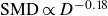 $\mathrm{SMD} \propto D^{-0.18}$
. Since varying
$\mathrm{SMD} \propto D^{-0.18}$
. Since varying
 $D$
is equivalent to varying the transverse dimension of the jet in the present study, i.e.
$D$
is equivalent to varying the transverse dimension of the jet in the present study, i.e.
 $\textit{AR}$
, while maintaining similar jet flow conditions. From the present experimental spray core data, it is observed that
$\textit{AR}$
, while maintaining similar jet flow conditions. From the present experimental spray core data, it is observed that
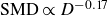 $\mathrm{SMD} \propto D^{-0.17}$
, indicating that an increase in
$\mathrm{SMD} \propto D^{-0.17}$
, indicating that an increase in
 $\textit{AR}$
leads to lower SMD, which is in line with the correlation of Amighi & Ashgriz (Reference Amighi and Ashgriz2019).
$\textit{AR}$
leads to lower SMD, which is in line with the correlation of Amighi & Ashgriz (Reference Amighi and Ashgriz2019).
Moreover, irrespective of the streamwise distance, the measured SMD for the spray with
 $\textit{AR} = 3.3$
near the tunnel floor is significantly higher than that for
$\textit{AR} = 3.3$
near the tunnel floor is significantly higher than that for
 $\textit{AR} = 0.3$
and
$\textit{AR} = 0.3$
and
 $\textit{AR} = 1$
. This is most likely due to the early breakup (figure 7), and large bending of the
$\textit{AR} = 1$
. This is most likely due to the early breakup (figure 7), and large bending of the
 $\textit{AR} = 3.3$
jet by the cross-flow. The larger droplets/liquid ligaments entrain into the low-velocity boundary layer near the tunnel floor. Subsequently, these droplets undergo a less intense secondary atomisation along the streamwise direction. Smaller droplets (more susceptible to the surrounding airflow) reach the tunnel floor for the sprays with
$\textit{AR} = 3.3$
jet by the cross-flow. The larger droplets/liquid ligaments entrain into the low-velocity boundary layer near the tunnel floor. Subsequently, these droplets undergo a less intense secondary atomisation along the streamwise direction. Smaller droplets (more susceptible to the surrounding airflow) reach the tunnel floor for the sprays with
 $\textit{AR} = 0.3$
and
$\textit{AR} = 0.3$
and
 $\textit{AR} = 1$
due to the delayed jet breakup and lifting of the spray plume from the tunnel wall. At downstream locations (
$\textit{AR} = 1$
due to the delayed jet breakup and lifting of the spray plume from the tunnel wall. At downstream locations (
 $x/D = 90$
and 115), the earlier larger droplets undergo secondary atomisation, resulting in the observed reduction in the SMD. It is observed from the instantaneous images (figure 4) that the lower part of the spray plume region in the case of
$x/D = 90$
and 115), the earlier larger droplets undergo secondary atomisation, resulting in the observed reduction in the SMD. It is observed from the instantaneous images (figure 4) that the lower part of the spray plume region in the case of
 $\textit{AR}$
= 1 (figure 4
b) contains relatively smaller droplets compared with those in the case of
$\textit{AR}$
= 1 (figure 4
b) contains relatively smaller droplets compared with those in the case of
 $\textit{AR}$
= 0.3 (figure 4
a). This is due to the difference in atomisation mechanism near the leeward side of the jet exit, as already discussed. The formation of denser spray on the leeward side (
$\textit{AR}$
= 0.3 (figure 4
a). This is due to the difference in atomisation mechanism near the leeward side of the jet exit, as already discussed. The formation of denser spray on the leeward side (
 $y/h_d$
< 0.5) due to the vigorous mass stripping in the case of
$y/h_d$
< 0.5) due to the vigorous mass stripping in the case of
 $\textit{AR}$
= 0.3 can lead to early fragmentation of ligaments or droplets in the spray plume. These fragmented droplets or ligaments are in continuous interaction with the low-speed boundary layer fluid near the tunnel floor as well as the lower momentum cross-flow fluid (caused by a stronger shockwave). Such delayed breakup in spray droplets causes the presence of larger droplets (higher SMD) at these heights (
$\textit{AR}$
= 0.3 can lead to early fragmentation of ligaments or droplets in the spray plume. These fragmented droplets or ligaments are in continuous interaction with the low-speed boundary layer fluid near the tunnel floor as well as the lower momentum cross-flow fluid (caused by a stronger shockwave). Such delayed breakup in spray droplets causes the presence of larger droplets (higher SMD) at these heights (
 $y/h_d$
< 0.5) of the downstream measurement stations (figure 24
i). In contrast, reduced mass stripping in the case of
$y/h_d$
< 0.5) of the downstream measurement stations (figure 24
i). In contrast, reduced mass stripping in the case of
 $\textit{AR}$
= 1 jet results in the formation of a dilute spray region in the downstream measurement locations at lower transverse heights (
$\textit{AR}$
= 1 jet results in the formation of a dilute spray region in the downstream measurement locations at lower transverse heights (
 $y/h_d$
< 0.5) without significant presence of larger droplets.
$y/h_d$
< 0.5) without significant presence of larger droplets.
The variation of mean streamwise velocity (
 $U$
), measured using the PTV technique, along the transverse direction for the sprays with different
$U$
), measured using the PTV technique, along the transverse direction for the sprays with different
 $\textit{AR}$
at different locations in the spray plume (
$\textit{AR}$
at different locations in the spray plume (
 $x/D$
= 60, 90 and 115), is shown in figure 24(ii). The cross-stream variation of
$x/D$
= 60, 90 and 115), is shown in figure 24(ii). The cross-stream variation of
 $U$
exhibits a C-shaped curve with a minimum of approximately 0.35
$U$
exhibits a C-shaped curve with a minimum of approximately 0.35
 $U_\infty$
and 0.4
$U_\infty$
and 0.4
 $U_\infty$
at
$U_\infty$
at
 $y = 0.5 h_d$
for
$y = 0.5 h_d$
for
 $\textit{AR} = 0.3$
and 1, respectively. The larger droplets present at this region (see figures 21
i and 21
ii) have higher inertia; hence, move with reduced velocities. However, for
$\textit{AR} = 0.3$
and 1, respectively. The larger droplets present at this region (see figures 21
i and 21
ii) have higher inertia; hence, move with reduced velocities. However, for
 $\textit{AR} = 3.3$
, the minimum mean streamwise velocity (0.35
$\textit{AR} = 3.3$
, the minimum mean streamwise velocity (0.35
 $U_\infty$
) is observed near the tunnel floor. For all jets, beyond
$U_\infty$
) is observed near the tunnel floor. For all jets, beyond
 $y = 0.5h_d$
, the value of
$y = 0.5h_d$
, the value of
 $U$
rises with the increase in
$U$
rises with the increase in
 $y$
inside the spray plume and reaches the maximum
$y$
inside the spray plume and reaches the maximum
 $U$
of approximately 0.85
$U$
of approximately 0.85
 $U_\infty$
at the top spray edge. From this, it can be concluded that the entire spray plume experiences a non-uniform velocity in the transverse direction, which most likely arises from the bow shock formation in the supersonic cross-flow.
$U_\infty$
at the top spray edge. From this, it can be concluded that the entire spray plume experiences a non-uniform velocity in the transverse direction, which most likely arises from the bow shock formation in the supersonic cross-flow.
To summarise, we see substantial differences in the droplet number, volume and velocity p.d.f.s in the core of the spray as the orifice
 $\textit{AR}$
is varied, with some of the key points being shown in table 7. In the case of
$\textit{AR}$
is varied, with some of the key points being shown in table 7. In the case of
 $\textit{AR}=0.3$
, although we see RT waves near the stagnation region of the injected jet, the primary atomisation likely is initiated by KH waves on the deformed lateral sides, leading to tongues of liquid that protrude into the cross-flow (as reported by Varga et al. (Reference Varga, Lasheras and Hopfinger2003)) that are broken by RTI. This results in a substantial increase in the contribution of liquid volume in the larger droplets after being fragmented due to mass stripping from the lateral sides as seen in the volume p.d.f. (see figure 21
c). Consequently, the volume p.d.f. in this case is significantly different from the other
$\textit{AR}=0.3$
, although we see RT waves near the stagnation region of the injected jet, the primary atomisation likely is initiated by KH waves on the deformed lateral sides, leading to tongues of liquid that protrude into the cross-flow (as reported by Varga et al. (Reference Varga, Lasheras and Hopfinger2003)) that are broken by RTI. This results in a substantial increase in the contribution of liquid volume in the larger droplets after being fragmented due to mass stripping from the lateral sides as seen in the volume p.d.f. (see figure 21
c). Consequently, the volume p.d.f. in this case is significantly different from the other
 $\textit{AR}$
cases with it having a broad peak centred at approximately 35
$\textit{AR}$
cases with it having a broad peak centred at approximately 35
 $\unicode{x03BC}$
m along with a higher SMD (27
$\unicode{x03BC}$
m along with a higher SMD (27
 $\unicode{x03BC}$
m) in the spray core. In the
$\unicode{x03BC}$
m) in the spray core. In the
 $\textit{AR}=1$
case, although RT waves are again present near the stagnation region of the injected jet, the primary atomisation would again result from KHI on the deformed small lateral sides (see figure 5) of the injected jet slice with RT that could occur subsequently (on the tongues) as in the
$\textit{AR}=1$
case, although RT waves are again present near the stagnation region of the injected jet, the primary atomisation would again result from KHI on the deformed small lateral sides (see figure 5) of the injected jet slice with RT that could occur subsequently (on the tongues) as in the
 $\textit{AR}=0.3$
case. However, it is important to note that there are large quantitative differences in the volume p.d.f. for the
$\textit{AR}=0.3$
case. However, it is important to note that there are large quantitative differences in the volume p.d.f. for the
 $\textit{AR}=1$
case compared with the
$\textit{AR}=1$
case compared with the
 $\textit{AR}=0.3$
case. In particular, the volume p.d.f. peak in this
$\textit{AR}=0.3$
case. In particular, the volume p.d.f. peak in this
 $\textit{AR}=1$
case is much narrower and the peak shifts substantially to smaller values (25
$\textit{AR}=1$
case is much narrower and the peak shifts substantially to smaller values (25
 $\unicode{x03BC}$
m), with the SMD in the core consequently also being reduced significantly reduced to 21
$\unicode{x03BC}$
m), with the SMD in the core consequently also being reduced significantly reduced to 21
 $\unicode{x03BC}$
m compared with the 27
$\unicode{x03BC}$
m compared with the 27
 $\unicode{x03BC}$
m for the
$\unicode{x03BC}$
m for the
 $\textit{AR}$
= 0.3 case. In contrast, in the case of
$\textit{AR}$
= 0.3 case. In contrast, in the case of
 $\textit{AR}=3.3$
, the atomisation occurs directly through RT instability in a catastrophic manner as observed by Joseph et al. (Reference Joseph, Belanger and Beavers1999). This results in the peak of the volume p.d.f. reducing to even lower droplet diameters (18
$\textit{AR}=3.3$
, the atomisation occurs directly through RT instability in a catastrophic manner as observed by Joseph et al. (Reference Joseph, Belanger and Beavers1999). This results in the peak of the volume p.d.f. reducing to even lower droplet diameters (18
 $\unicode{x03BC}$
m), and the relatively direct clear atomisation by RT results in the SMD (18
$\unicode{x03BC}$
m), and the relatively direct clear atomisation by RT results in the SMD (18
 $\unicode{x03BC}$
m) also being close to the peak in the volume p.d.f. (18
$\unicode{x03BC}$
m) also being close to the peak in the volume p.d.f. (18
 $\unicode{x03BC}$
m). Further, it may be noted that the catastrophic break up directly by RT in this
$\unicode{x03BC}$
m). Further, it may be noted that the catastrophic break up directly by RT in this
 $\textit{AR}=3.3$
case also results in early breakup of the liquid jet as seen in the relatively large droplet velocities as seen in the velocity p.d.f. (see figure 21
d).
$\textit{AR}=3.3$
case also results in early breakup of the liquid jet as seen in the relatively large droplet velocities as seen in the velocity p.d.f. (see figure 21
d).
Effect of AR on
 $\lambda /b$
, peak in the volume PDF, SMD and the destabilisation mechanism.
$\lambda /b$
, peak in the volume PDF, SMD and the destabilisation mechanism.

5.2. Temporal variation of spray characteristics
Having obtained the long-time averaged information on droplet size distribution, we shall now focus our attention on the unsteadiness involved in the spray characteristics which are significantly altered by AR. These are caused by surface wave-induced shock corrugations in the spray core for the
 $\textit{AR}=0.3$
case and at the spray edge for all
$\textit{AR}=0.3$
case and at the spray edge for all
 $\textit{AR}$
cases primarily due to the unsteadiness in jet penetration height that is mainly driven by the boundary layer velocity fluctuations as discussed in § 4.3.
$\textit{AR}$
cases primarily due to the unsteadiness in jet penetration height that is mainly driven by the boundary layer velocity fluctuations as discussed in § 4.3.
Temporal variation of SMD and
 $U$
at the (i) core (
$U$
at the (i) core (
 $y/h_d = 0.5$
and
$y/h_d = 0.5$
and
 $x/D = 60$
) and (ii) edge (
$x/D = 60$
) and (ii) edge (
 $y/h_d = 1$
and
$y/h_d = 1$
and
 $x/D = 60$
) of the spray in supersonic cross-flow with (a)
$x/D = 60$
) of the spray in supersonic cross-flow with (a)
 $\textit{AR} = 0.3$
, (b)
$\textit{AR} = 0.3$
, (b)
 $\textit{AR} = 1$
and (c)
$\textit{AR} = 1$
and (c)
 $\textit{AR} = 3.3$
, and
$\textit{AR} = 3.3$
, and
 $J = 9.7$
.
$J = 9.7$
.

Figures 29(a) and figures 29(b) (Appendix B) show a sample pair of droplet images acquired at the core of the spray plume (
 $y/h_d = 0.5$
) and top edge (
$y/h_d = 0.5$
) and top edge (
 $y/h_d = 1$
) of the spray, respectively, for
$y/h_d = 1$
) of the spray, respectively, for
 $\textit{AR} = 0.3$
, and
$\textit{AR} = 0.3$
, and
 $J = 9.7$
at
$J = 9.7$
at
 $x/D = 60$
. These pairs of images are separated by a very large time difference of 66 ms, which essentially means that these are completely independent realisations of the spray. Note that the PDIA technique is able to size also non-spherical drops and for these, an area equivalent diameter is used. Furthermore, the PDIA exhibits a high dynamic range in drop size. Figures 29(a) (i and ii) clearly distinguish the number of droplets, droplet size and shape between the time instants at
$x/D = 60$
. These pairs of images are separated by a very large time difference of 66 ms, which essentially means that these are completely independent realisations of the spray. Note that the PDIA technique is able to size also non-spherical drops and for these, an area equivalent diameter is used. Furthermore, the PDIA exhibits a high dynamic range in drop size. Figures 29(a) (i and ii) clearly distinguish the number of droplets, droplet size and shape between the time instants at
 $y/h_d = 0.5$
for the spray with
$y/h_d = 0.5$
for the spray with
 $\textit{AR} = 0.3$
. A similar pattern but at a reduced scale is observed for
$\textit{AR} = 0.3$
. A similar pattern but at a reduced scale is observed for
 $\textit{AR} = 1$
and 3.3. Although highly nonlinear spray dynamics in the form of intense ligaments/droplets formation, which undergo stretching followed by a breakup, is taking place by the time the spray arrives at the present measurement station, one of the possible reasons for this peculiar unsteady behaviour observed in the case of the
$\textit{AR} = 1$
and 3.3. Although highly nonlinear spray dynamics in the form of intense ligaments/droplets formation, which undergo stretching followed by a breakup, is taking place by the time the spray arrives at the present measurement station, one of the possible reasons for this peculiar unsteady behaviour observed in the case of the
 $\textit{AR} = 0.3$
jet could be due to the increased fluctuations of instantaneous formation of large-scale windward surface wavelengths resulting in variations in curvature/strength of the stronger bumpy shocks with time (see figures 8
ai and 8
aii). The quantified difference in this unsteady spray behaviour between the
$\textit{AR} = 0.3$
jet could be due to the increased fluctuations of instantaneous formation of large-scale windward surface wavelengths resulting in variations in curvature/strength of the stronger bumpy shocks with time (see figures 8
ai and 8
aii). The quantified difference in this unsteady spray behaviour between the
 $\textit{AR}$
s will be discussed in detail next.
$\textit{AR}$
s will be discussed in detail next.
At the spray edge (
 $y/h_d = 1$
), due to the continuous interaction of the spray plume with the oncoming supersonic air, the droplet size (narrower) and shape are similar between the instants, but there is a wide range in the number of droplets between the instants (figures 29
biii and 29
biv). Irrespective of AR, the unsteadiness in jet penetration heights governs the variations in droplet shape, size and number at all cross-streamwise directions.
$y/h_d = 1$
), due to the continuous interaction of the spray plume with the oncoming supersonic air, the droplet size (narrower) and shape are similar between the instants, but there is a wide range in the number of droplets between the instants (figures 29
biii and 29
biv). Irrespective of AR, the unsteadiness in jet penetration heights governs the variations in droplet shape, size and number at all cross-streamwise directions.
To quantify the unsteady behaviour showcased by the previous images, SMD and mean streamwise velocity (
 $U$
) for each instance are determined by identifying the droplet size and its velocity at each instant. Figures 25(i) and 25(ii) illustrate the temporal variation of SMD and
$U$
) for each instance are determined by identifying the droplet size and its velocity at each instant. Figures 25(i) and 25(ii) illustrate the temporal variation of SMD and
 $U/U_\infty$
at
$U/U_\infty$
at
 $y/h_d = 0.5$
and 1 for
$y/h_d = 0.5$
and 1 for
 $\textit{AR} = 0.3$
, 1 and 3.3. In the core of the spray plume (figure 25
i) for
$\textit{AR} = 0.3$
, 1 and 3.3. In the core of the spray plume (figure 25
i) for
 $\textit{AR} = 0.3$
, the SMD (10–45)
$\textit{AR} = 0.3$
, the SMD (10–45)
 $\unicode{x03BC}$
m and
$\unicode{x03BC}$
m and
 $U/U_\infty$
(0.2–0.45) vary over a larger range when compared with other
$U/U_\infty$
(0.2–0.45) vary over a larger range when compared with other
 $\textit{AR}$
cases. Also, these variations are much higher when compared with variations in long-time averaged SMD and
$\textit{AR}$
cases. Also, these variations are much higher when compared with variations in long-time averaged SMD and
 $U/U_\infty$
among the stations, as well as with
$U/U_\infty$
among the stations, as well as with
 $\textit{AR}$
. A substantial reduction of instantaneous difference in maximum and minimum SMD values was found with an increase in
$\textit{AR}$
. A substantial reduction of instantaneous difference in maximum and minimum SMD values was found with an increase in
 $\textit{AR}$
i.e. from 35
$\textit{AR}$
i.e. from 35
 $\unicode{x03BC}$
m (AR = 0.3) to 20
$\unicode{x03BC}$
m (AR = 0.3) to 20
 $\unicode{x03BC}$
m (AR = 3.3) because of the significant reduction in the variations in size of the windward liquid structures; hence, the shock bumpiness. At the spray edge, the temporal variation in SMD (10–25)
$\unicode{x03BC}$
m (AR = 3.3) because of the significant reduction in the variations in size of the windward liquid structures; hence, the shock bumpiness. At the spray edge, the temporal variation in SMD (10–25)
 $\unicode{x03BC}$
m and
$\unicode{x03BC}$
m and
 $U/U_\infty$
(0.7–0.9) exhibits significant reduction irrespective of the
$U/U_\infty$
(0.7–0.9) exhibits significant reduction irrespective of the
 $\textit{AR}$
, as shown in figure 25(ii). These fluctuations are attributed to the variations in the spray edge position/penetration height of the liquid jet between the instants (see figure 17). This is likely related to shock boundary layer interactions and the resulting low-frequency fluctuations that are known to occur with typical frequency (
$\textit{AR}$
, as shown in figure 25(ii). These fluctuations are attributed to the variations in the spray edge position/penetration height of the liquid jet between the instants (see figure 17). This is likely related to shock boundary layer interactions and the resulting low-frequency fluctuations that are known to occur with typical frequency (
 $f$
) represented by a Strouhal number, St =
$f$
) represented by a Strouhal number, St =
 $f\delta /U_\infty \sim$
0.01 (Clemens & Narayanaswamy Reference Clemens and Narayanaswamy2014), where
$f\delta /U_\infty \sim$
0.01 (Clemens & Narayanaswamy Reference Clemens and Narayanaswamy2014), where
 $\delta$
and
$\delta$
and
 $U_\infty$
represent the incoming boundary-layer thickness and the free stream velocity, respectively. In the case of liquid jet injection into supersonic cross-flow, Medipati et al. (Reference Medipati, Deivandren and Govardhan2023) have shown that this can lead to naturally induced pressure and mass flow fluctuations in the liquid line at
$U_\infty$
represent the incoming boundary-layer thickness and the free stream velocity, respectively. In the case of liquid jet injection into supersonic cross-flow, Medipati et al. (Reference Medipati, Deivandren and Govardhan2023) have shown that this can lead to naturally induced pressure and mass flow fluctuations in the liquid line at
 $f\delta /U_\infty \sim$
0.01, which can lead to significant unsteadiness in the penetration height and drop sizes.
$f\delta /U_\infty \sim$
0.01, which can lead to significant unsteadiness in the penetration height and drop sizes.
A quantitative correlation analysis is performed between the instantaneous values of SMD, and
 $U/U_\infty$
for different aspect ratios and spray plume stations. The correlation values fall in the range of -0.5 to -0.7. It indicates that an instant with larger droplets leads to higher SMD, resulting in lower streamwise droplet velocity (
$U/U_\infty$
for different aspect ratios and spray plume stations. The correlation values fall in the range of -0.5 to -0.7. It indicates that an instant with larger droplets leads to higher SMD, resulting in lower streamwise droplet velocity (
 $U$
). This strongly suggests that the values of SMD and
$U$
). This strongly suggests that the values of SMD and
 $U/U_\infty$
are highly correlated.
$U/U_\infty$
are highly correlated.
In summary, the unsteadiness in droplet sizes in the spray core, particularly seen at
 $\textit{AR}=0.3$
case, is seen to be related to the large wavelength surface waves and the associated shock corrugations. However, large variations in droplet sizes in time seen at the spray edge in all the
$\textit{AR}=0.3$
case, is seen to be related to the large wavelength surface waves and the associated shock corrugations. However, large variations in droplet sizes in time seen at the spray edge in all the
 $\textit{AR}$
cases are seen to be related to the unsteadiness in jet penetration height induced by low- and high-speed streaks within the boundary layer interacting with the shock foot.
$\textit{AR}$
cases are seen to be related to the unsteadiness in jet penetration height induced by low- and high-speed streaks within the boundary layer interacting with the shock foot.
6. Summary and conclusions
In the present work, we have experimentally investigated the flow field interactions when a liquid jet is injected transversely into supersonic cross-flow (
 $M_\infty$
= 2.5). The primary focus of the present study was to understand the influence of orifice aspect ratio (AR) on the formation of surface waves on the windward side, shock structures, jet penetration height and the atomisation mechanism along with their unsteady aspects. These studies were carried out for three orifice aspect ratios (
$M_\infty$
= 2.5). The primary focus of the present study was to understand the influence of orifice aspect ratio (AR) on the formation of surface waves on the windward side, shock structures, jet penetration height and the atomisation mechanism along with their unsteady aspects. These studies were carried out for three orifice aspect ratios (
 $\textit{AR}=b/a$
), namely, 0.3, 1 and 3.3, where
$\textit{AR}=b/a$
), namely, 0.3, 1 and 3.3, where
 $\textit{AR}$
is defined as the ratio of the orifice spanwise dimension (
$\textit{AR}$
is defined as the ratio of the orifice spanwise dimension (
 $b$
) to streamwise dimension (
$b$
) to streamwise dimension (
 $a$
). The study clearly shows that the orifice
$a$
). The study clearly shows that the orifice
 $\textit{AR}$
has a significant effect on different aspects of the flow field and spray such as surface wavelengths (
$\textit{AR}$
has a significant effect on different aspects of the flow field and spray such as surface wavelengths (
 $\lambda /b$
), penetration height (
$\lambda /b$
), penetration height (
 $\overline {h}/D$
) and its unsteadiness, shock locations (
$\overline {h}/D$
) and its unsteadiness, shock locations (
 $y_s/D$
), lateral jet spread (
$y_s/D$
), lateral jet spread (
 $\overline {W}/b$
), and droplet size (SMD) and velocity in the spray core, as summarised in figure 26 and discussed next.
$\overline {W}/b$
), and droplet size (SMD) and velocity in the spray core, as summarised in figure 26 and discussed next.
Plots of variation with AR in (a) surface wavelength (
 $\lambda /b$
), (b) penetration height (
$\lambda /b$
), (b) penetration height (
 $\overline {h}/D$
), (c) shock locations (
$\overline {h}/D$
), (c) shock locations (
 $y_s/D$
), (d) unsteadiness in penetration height (
$y_s/D$
), (d) unsteadiness in penetration height (
 $\sigma _{{h}}/\overline {h}$
), (e) lateral jet spread (
$\sigma _{{h}}/\overline {h}$
), (e) lateral jet spread (
 $\overline {W}/b$
) and (f) Sauter mean diameter (SMD) and droplet velocity (
$\overline {W}/b$
) and (f) Sauter mean diameter (SMD) and droplet velocity (
 $U/U_\infty$
) in the spray core.
$U/U_\infty$
) in the spray core.

Liquid jets, when injected into supersonic cross-flow, are prone to instability due to the rapid acceleration of the liquid jet by the high-speed air because of the well-known Rayleigh–Taylor instability (Taylor Reference Taylor1950). The Kelvin–Helmholtz (KH) instability can also be important as seen in coaxial liquid jet atomisation studies (Varga et al. Reference Varga, Lasheras and Hopfinger2003). In the present study, variation in orifice AR leads to large changes in the frontal and lateral area of the liquid jet as it interacts with the high-speed air. This has resulted in significant variation in the primary atomisation mechanism of the injected liquid jet.
In the case of
 $\textit{AR}$
= 0.3, the surface waves formed on the windward side have a larger wavelength (
$\textit{AR}$
= 0.3, the surface waves formed on the windward side have a larger wavelength (
 $\lambda /b$
), when compared with those for
$\lambda /b$
), when compared with those for
 $\textit{AR}$
= 1 (figure 26
a). This is due to the reduced acceleration of the liquid jet by the cross-flow fluid due to the lower drag because of the reduced frontal area of the jet. The resulting large wavelength liquid surface deformations lead to large-scale corrugations in the upstream shock that vary with time. This triggers strong unsteadiness in the flow field within the spray core, which can be seen in the droplet sizes downstream. The primary atomisation route in this case, is however likely initiated by KH waves on the already deformed lateral sides of the liquid jet by the windward stagnation pressure, which leads to mass stripping from the jet surface in the form of liquid ligaments/tongues. These ligaments/tongues will be strongly accelerated by the surrounding high-speed air, leading to the formation of a spray due to the RTI. This is closely related to the well-studied coaxial liquid jet configuration (Varga et al. Reference Varga, Lasheras and Hopfinger2003). The presence of vigorous mass stripping from the lateral surface also resulted in lower penetration height (figure 26
b) as well as an increase in spanwise spray width (figure 26
e) when compared with
$\textit{AR}$
= 1 (figure 26
a). This is due to the reduced acceleration of the liquid jet by the cross-flow fluid due to the lower drag because of the reduced frontal area of the jet. The resulting large wavelength liquid surface deformations lead to large-scale corrugations in the upstream shock that vary with time. This triggers strong unsteadiness in the flow field within the spray core, which can be seen in the droplet sizes downstream. The primary atomisation route in this case, is however likely initiated by KH waves on the already deformed lateral sides of the liquid jet by the windward stagnation pressure, which leads to mass stripping from the jet surface in the form of liquid ligaments/tongues. These ligaments/tongues will be strongly accelerated by the surrounding high-speed air, leading to the formation of a spray due to the RTI. This is closely related to the well-studied coaxial liquid jet configuration (Varga et al. Reference Varga, Lasheras and Hopfinger2003). The presence of vigorous mass stripping from the lateral surface also resulted in lower penetration height (figure 26
b) as well as an increase in spanwise spray width (figure 26
e) when compared with
 $\textit{AR}$
= 1 due to a decrease in effective jet-to-cross-flow momentum flux ratio (Mashayek et al. Reference Mashayek, Jafari and Ashgriz2008; Broumand & Birouk Reference Broumand and Birouk2016b
). In sharp contrast, in the
$\textit{AR}$
= 1 due to a decrease in effective jet-to-cross-flow momentum flux ratio (Mashayek et al. Reference Mashayek, Jafari and Ashgriz2008; Broumand & Birouk Reference Broumand and Birouk2016b
). In sharp contrast, in the
 $\textit{AR}$
= 3.3 case, the higher exposed area jet in supersonic air resulted in the rapid acceleration of the jet. Hence, the surface RT waves that form have lower surface wavelengths and have higher surface deformations. This leads to the atomisation in this case being purely due to RT instability, resulting in the rapid catastrophic breakup of the liquid jet with sharper deflection of the jet by the cross-flow. Further, as the windward waves in this case have a much smaller wavelength, the bow shock is relatively free from large-scale corrugations and the resulting velocity field ahead of the liquid jet is smoother. It may be noted that the trend of a rapid decrease in surface wavelength with an increase in AR found from experimental measurements (figure 26
a) are in close agreement with the predictions of Rayleigh–Taylor linear instability analysis pertaining to the maximum growth rate. Further, these near-field differences among the ARs have significantly altered the column breakup location and the breakup time. The enhanced RT instability in the case of
$\textit{AR}$
= 3.3 case, the higher exposed area jet in supersonic air resulted in the rapid acceleration of the jet. Hence, the surface RT waves that form have lower surface wavelengths and have higher surface deformations. This leads to the atomisation in this case being purely due to RT instability, resulting in the rapid catastrophic breakup of the liquid jet with sharper deflection of the jet by the cross-flow. Further, as the windward waves in this case have a much smaller wavelength, the bow shock is relatively free from large-scale corrugations and the resulting velocity field ahead of the liquid jet is smoother. It may be noted that the trend of a rapid decrease in surface wavelength with an increase in AR found from experimental measurements (figure 26
a) are in close agreement with the predictions of Rayleigh–Taylor linear instability analysis pertaining to the maximum growth rate. Further, these near-field differences among the ARs have significantly altered the column breakup location and the breakup time. The enhanced RT instability in the case of
 $\textit{AR}$
= 3.3 exhibits the lower breakup location and time. The value of
$\textit{AR}$
= 3.3 exhibits the lower breakup location and time. The value of
 $t_b/ t^*$
found is inline with the droplet in supersonic flow studies (Hsiang & Faeth Reference Hsiang and Faeth1992), indicating the reminiscence in the atomisation mechanism between the transverse jet and droplet in supersonic flow.
$t_b/ t^*$
found is inline with the droplet in supersonic flow studies (Hsiang & Faeth Reference Hsiang and Faeth1992), indicating the reminiscence in the atomisation mechanism between the transverse jet and droplet in supersonic flow.
To understand the source of unsteadiness in the penetration height, PIV measurements were carried out upstream of the liquid jet. It was found that there was a large variation in the incoming boundary-layer thickness between the instants due to the presence of low/high-speed boundary streaks similar to Ganapathisubramani et al. (Reference Ganapathisubramani, Clemens and Dolling2007) and Murugan & Govardhan (Reference Murugan and Govardhan2016). The natural occurrence of these streaks inside the turbulent boundary layer creates a large variation in the total momentum of the cross-flow fluid (boundary layer + cross-flow) as encountered by the liquid jet between the instants. This triggers fluctuations in the jet penetration height, as discussed by Munuswamy & Govardhan (Reference Munuswamy and Govardhan2022). In the present study, variation in
 $\textit{AR}$
has significantly changed the unsteadiness in jet penetration height and shock position due to the difference in the interaction area and frontal-to-streak width ratio of the injected liquid jet with the oncoming turbulent boundary layer. It was observed that
$\textit{AR}$
has significantly changed the unsteadiness in jet penetration height and shock position due to the difference in the interaction area and frontal-to-streak width ratio of the injected liquid jet with the oncoming turbulent boundary layer. It was observed that
 $\textit{AR}$
= 3.3 (frontal to streak width ratio = 0.5) and
$\textit{AR}$
= 3.3 (frontal to streak width ratio = 0.5) and
 $\textit{AR}$
= 1 (frontal to streak width ratio = 0.27) show the highest and least unsteadiness due to the stronger and weaker interaction with the boundary-layer streaks, whose streamwise and spanwise length scales are 40
$\textit{AR}$
= 1 (frontal to streak width ratio = 0.27) show the highest and least unsteadiness due to the stronger and weaker interaction with the boundary-layer streaks, whose streamwise and spanwise length scales are 40
 $\delta$
and 0.5
$\delta$
and 0.5
 $\delta$
, respectively (Ganapathisubramani et al. Reference Ganapathisubramani, Clemens and Dolling2007).
$\delta$
, respectively (Ganapathisubramani et al. Reference Ganapathisubramani, Clemens and Dolling2007).
The differences in the atomisation mechanism of the injected liquid jet with
 $\textit{AR}$
have eventually altered the dispersion as well as distribution of droplets across the spray plume substantially. It was found that in the case of
$\textit{AR}$
have eventually altered the dispersion as well as distribution of droplets across the spray plume substantially. It was found that in the case of
 $\textit{AR}$
= 0.3, the droplets formed are larger as well as non-spherical with a significant fragmented liquid volume carried by the larger droplets associated with lower droplet velocities. As discussed earlier, this is consistent with the atomisation occurring primarily due to KHI along the lateral surfaces similar to Varga et al. (Reference Varga, Lasheras and Hopfinger2003), which leads to mass stripping from the jet surface in the form of liquid ligaments/tongues that may further breakup due to the RTI. In contrast, in the case of
$\textit{AR}$
= 0.3, the droplets formed are larger as well as non-spherical with a significant fragmented liquid volume carried by the larger droplets associated with lower droplet velocities. As discussed earlier, this is consistent with the atomisation occurring primarily due to KHI along the lateral surfaces similar to Varga et al. (Reference Varga, Lasheras and Hopfinger2003), which leads to mass stripping from the jet surface in the form of liquid ligaments/tongues that may further breakup due to the RTI. In contrast, in the case of
 $\textit{AR}$
= 3.3, the droplets formed are smaller as well as more spherical as indicated by the fact that the fragmented liquid volume is mostly carried by smaller droplets (from volume p.d.f.) with higher droplet velocities (from velocity p.d.f.). These differences in atomisation mechanism with AR have significantly altered the profiles of Sauter mean diameter (SMD) and mean streamwise droplet velocity (
$\textit{AR}$
= 3.3, the droplets formed are smaller as well as more spherical as indicated by the fact that the fragmented liquid volume is mostly carried by smaller droplets (from volume p.d.f.) with higher droplet velocities (from velocity p.d.f.). These differences in atomisation mechanism with AR have significantly altered the profiles of Sauter mean diameter (SMD) and mean streamwise droplet velocity (
 $U$
/
$U$
/
 $U_\infty$
) along the cross-streamwise direction. The smaller surface wavelength with more intense surface deformations seen in this
$U_\infty$
) along the cross-streamwise direction. The smaller surface wavelength with more intense surface deformations seen in this
 $\textit{AR}=3.3$
case, along with the dominant contribution of the atomised liquid volume by the smaller droplets (lower SMD), indicates that the atomisation is purely due to RTI, as reported by Joseph et al. (Reference Joseph, Belanger and Beavers1999).
$\textit{AR}=3.3$
case, along with the dominant contribution of the atomised liquid volume by the smaller droplets (lower SMD), indicates that the atomisation is purely due to RTI, as reported by Joseph et al. (Reference Joseph, Belanger and Beavers1999).
Substantial unsteadiness is also seen in the drop sizes. This is particularly clear within the spray core for the
 $\textit{AR}=0.3$
case, and is seen to be related to the large wavelength surface waves and the associated shock corrugations. However, large variations in droplet sizes in time seen at the spray edge in all the
$\textit{AR}=0.3$
case, and is seen to be related to the large wavelength surface waves and the associated shock corrugations. However, large variations in droplet sizes in time seen at the spray edge in all the
 $\textit{AR}$
cases are seen to be related to the unsteadiness in jet penetration height induced by low- and high-speed streaks within the boundary layer interacting with the shock foot.
$\textit{AR}$
cases are seen to be related to the unsteadiness in jet penetration height induced by low- and high-speed streaks within the boundary layer interacting with the shock foot.
In summary, the present study shows the importance of the orifice
 $\textit{AR}$
on the flow around and the spray downstream of liquid injection into supersonic cross-flow, which can have consequences for applications where such flows occur.
$\textit{AR}$
on the flow around and the spray downstream of liquid injection into supersonic cross-flow, which can have consequences for applications where such flows occur.
Funding
The authors acknowledge support from the JATP programme at IISc for financial support of the experimental work. This research was supported by the SERB Visiting Advanced Joint Research Faculty Scheme (VAJRA) of the Indian Department of Science and Technology (DST) for C.T.
Declaration of interests
The authors report no conflict of interest.
Appendix A
In this Appendix, we present the details of the simple force balance model used to predict the windward edge trajectory of the jet when injected into supersonic cross-flow for different AR and J by modifying the models developed for existing subsonic studies (Wu et al. Reference Wu, Kirkendall, Fuller and Nejad1997; Ashgriz Reference Ashgriz2011).
The following are the assumptions used in the present model:
-
(i) deformation of the liquid fluid element is absent;
-
(ii) mass losses are neglected, e.g. through mass stripping;
-
(iii) the vertical velocity of the liquid fluid elements remains constant and equal to the exit velocity from the orifice;
-
(iv) forces due to gravity, surface tension and viscosity are neglected.
First, a fluid element with an area averaged vertical velocity of
 $U_j$
(injection velocity) that starts at a time
$U_j$
(injection velocity) that starts at a time
 $t = 0$
from the orifice exit is considered. At any given instant/location, the fluid element experiences a drag force (
$t = 0$
from the orifice exit is considered. At any given instant/location, the fluid element experiences a drag force (
 $F_D$
) in the streamwise direction due to the aerodynamic force exerted by the oncoming free stream air as illustrated in figure 14. This results in acceleration of the fluid (
$F_D$
) in the streamwise direction due to the aerodynamic force exerted by the oncoming free stream air as illustrated in figure 14. This results in acceleration of the fluid (
 $a_x$
) in the same direction. This determines the instantaneous streamwise velocity attained by the fluid element. With the known velocity information in both the streamwise and transverse directions, the displacement of the fluid element is determined according to the following equations. The
$a_x$
) in the same direction. This determines the instantaneous streamwise velocity attained by the fluid element. With the known velocity information in both the streamwise and transverse directions, the displacement of the fluid element is determined according to the following equations. The
 $x$
-direction momentum equation for this fluid element is written as
$x$
-direction momentum equation for this fluid element is written as
 \begin{equation} \Sigma F_x = ma_x = F_{D} \end{equation}
assuming that only the drag force acts on the fluid element in the
 $x$
-direction, where
$x$
-direction, where
 $F_{D}$
is the drag force due to the free stream air, and
$F_{D}$
is the drag force due to the free stream air, and
 $m$
and
$m$
and
 $a_x$
represent mass and acceleration in the
$a_x$
represent mass and acceleration in the
 $x$
-direction, respectively. Substituting the equation for drag of the fluid element into (A1) results in
$x$
-direction, respectively. Substituting the equation for drag of the fluid element into (A1) results in
 \begin{equation} \frac {1}{2}C_{D}\rho _2 U_2^2 A_f = \rho _l V_l \frac {{\rm d}U_x}{{\rm d}t}, \end{equation}
where
 $C_{D}$
represents the drag coefficient,
$C_{D}$
represents the drag coefficient,
 $\rho _2$
,
$\rho _2$
,
 $U_2$
represent the density and velocity of the free stream post-shock air, and
$U_2$
represent the density and velocity of the free stream post-shock air, and
 $A_f$
,
$A_f$
,
 $V_l$
,
$V_l$
,
 $U_x$
represent the frontal area, volume and the streamwise velocity of the fluid element, respectively. In the present study, jet injection into supersonic cross-flow at different
$U_x$
represent the frontal area, volume and the streamwise velocity of the fluid element, respectively. In the present study, jet injection into supersonic cross-flow at different
 $\textit{AR}$
resulted in different
$\textit{AR}$
resulted in different
 $ A_f$
and
$ A_f$
and
 $C_D$
as given in table 8. The assumed values of
$C_D$
as given in table 8. The assumed values of
 $C_{D}$
in this table correspond to values obtained experimentally in the case of supersonic flow over solid bodies of different aspect ratios by Gowen & Perkins (Reference Gowen and Perkins1953) and Heddleson et al. (Reference Heddleson, Brown and Cliffe1957). Using the inviscid shock relations over mean shock traces obtained from the experimental studies, the values/variation of
$C_{D}$
in this table correspond to values obtained experimentally in the case of supersonic flow over solid bodies of different aspect ratios by Gowen & Perkins (Reference Gowen and Perkins1953) and Heddleson et al. (Reference Heddleson, Brown and Cliffe1957). Using the inviscid shock relations over mean shock traces obtained from the experimental studies, the values/variation of
 $\rho _2$
,
$\rho _2$
,
 $U_2$
(after the shock) experienced by the fluid element are determined. Integrating (A2) results in
$U_2$
(after the shock) experienced by the fluid element are determined. Integrating (A2) results in
 \begin{equation} U_{(x,i)}=U_{(x,i-1)}+\left [\frac {0.5C_D \rho _{2i} U_{2i}^2 A_f}{\rho _l V_l}\right]t, \end{equation}
where ‘
 $i$
’ represents time step of the fluid element. By substituting
$i$
’ represents time step of the fluid element. By substituting
 $U_x = \mathrm{d}x/\mathrm{d}t$
, the streamwise location of the fluid element can be determined through integration of (A3):
$U_x = \mathrm{d}x/\mathrm{d}t$
, the streamwise location of the fluid element can be determined through integration of (A3):
 \begin{equation} x_i=x_{i-1}+\left [\frac {0.5C_D \rho _{2i} U_{2i}^2 A_f}{\rho _l V_l}\right]t^2. \end{equation}
As the vertical velocity of the fluid element is constant, the ‘
 $t$
’ is calculated as
$t$
’ is calculated as
 \begin{equation} t=\frac {y_i - y_{i-1}}{U_j}.\end{equation}
Solving (A4) and (A5) together enables the determination of the instantaneous
 $x$
and
$x$
and
 $y$
locations of the fluid element. Tracing the
$y$
locations of the fluid element. Tracing the
 $x$
and
$x$
and
 $y$
locations of the fluid element with time results in the windward edge trajectory of the liquid jet as presented in § 4.2.
$y$
locations of the fluid element with time results in the windward edge trajectory of the liquid jet as presented in § 4.2.
Values of
 $A_f$
,
$A_f$
,
 $C_D$
and
$C_D$
and
 $V_l$
used in the present model for different values of
$V_l$
used in the present model for different values of
 $\textit{AR}$
.
$\textit{AR}$
.

A typical instantaneous visualisation of the spray in supersonic cross-flow for
 $\textit{AR} = 1$
and
$\textit{AR} = 1$
and
 $J = 9.7$
. The spatial locations along the cross-stream direction at
$J = 9.7$
. The spatial locations along the cross-stream direction at
 $x/D = 60$
for the measurement of drop size distribution using PDIA are highlighted.
$x/D = 60$
for the measurement of drop size distribution using PDIA are highlighted.

Appendix B
In this appendix, we present sample images of the instantaneous visualisations for the PDIA measurements for different
 $\textit{AR}$
, locations and at different times. A sample instantaneous spray image highlighting the vertical measurement locations (different
$\textit{AR}$
, locations and at different times. A sample instantaneous spray image highlighting the vertical measurement locations (different
 $y/D$
) at
$y/D$
) at
 $x/D = 60$
in the spray, identified by white dots, is shown in figure 27 for
$x/D = 60$
in the spray, identified by white dots, is shown in figure 27 for
 $\textit{AR} = 1$
. These locations are marked as A, B, C, D and E for easy identification going from the lower wall (A) to the spray edge (E), with the spray core corresponding to the location (C). At each station, a large number of (approximately 500) instantaneous spray droplet images are acquired and used for the statistical analysis. The details of performing the experiment, as well as the process of quantification of spray characteristics like drop size and velocities using the PDIA technique, are explained in detail in our previous work (Medipati et al. Reference Medipati, Deivandren and Govardhan2023) and by Sinha et al. (Reference Sinha, Prakash, Mohan and Ravikrishna2015).
$\textit{AR} = 1$
. These locations are marked as A, B, C, D and E for easy identification going from the lower wall (A) to the spray edge (E), with the spray core corresponding to the location (C). At each station, a large number of (approximately 500) instantaneous spray droplet images are acquired and used for the statistical analysis. The details of performing the experiment, as well as the process of quantification of spray characteristics like drop size and velocities using the PDIA technique, are explained in detail in our previous work (Medipati et al. Reference Medipati, Deivandren and Govardhan2023) and by Sinha et al. (Reference Sinha, Prakash, Mohan and Ravikrishna2015).
The sample droplet images acquired at stations ‘C’ and ‘E’ are shown in figures 28(a) and 28(b), respectively, for different
 $\textit{AR}$
and
$\textit{AR}$
and
 $J$
= 9.7. Figures 29(a) and 29(b) shows the unsteadiness in the formation of the droplets at
$J$
= 9.7. Figures 29(a) and 29(b) shows the unsteadiness in the formation of the droplets at
 $y/h_d = 0.5$
and
$y/h_d = 0.5$
and
 $y/h_d = 1$
for the
$y/h_d = 1$
for the
 $\textit{AR}$
= 0.3 and
$\textit{AR}$
= 0.3 and
 $J$
= 9.7. A detailed analysis highlighting the effect of
$J$
= 9.7. A detailed analysis highlighting the effect of
 $\textit{AR}$
on the distribution of droplets and their velocity, along with their mean SMD and
$\textit{AR}$
on the distribution of droplets and their velocity, along with their mean SMD and
 $U/U_\infty$
trends, followed by the instantaneous variation of SMD and
$U/U_\infty$
trends, followed by the instantaneous variation of SMD and
 $U/U_\infty$
are discussed in § 5.
$U/U_\infty$
are discussed in § 5.
(a) High-resolution images of spray droplets at
 $y/h_d$
= 0.5 (station ‘C’) for (i)
$y/h_d$
= 0.5 (station ‘C’) for (i)
 $\textit{AR} = 0.3$
, (ii)
$\textit{AR} = 0.3$
, (ii)
 $\textit{AR} = 1$
and (iii)
$\textit{AR} = 1$
and (iii)
 $\textit{AR} = 3.3$
. (b) High-resolution images of spray droplets at
$\textit{AR} = 3.3$
. (b) High-resolution images of spray droplets at
 $y/h_d$
= 1 (station ‘E’) for (iv)
$y/h_d$
= 1 (station ‘E’) for (iv)
 $\textit{AR} = 0.3$
, (v)
$\textit{AR} = 0.3$
, (v)
 $\textit{AR} = 1$
and (vi)
$\textit{AR} = 1$
and (vi)
 $\textit{AR} = 3.3$
. All the measurements correspond to
$\textit{AR} = 3.3$
. All the measurements correspond to
 $x/D$
= 60 and
$x/D$
= 60 and
 $J$
= 9.7.
$J$
= 9.7.

(a) Instantaneous visualisations of spray droplets captured in the core (
 $y/h_d = 0.5$
) and (b) instantaneous visualisations of spray droplets captured at the edge (
$y/h_d = 0.5$
) and (b) instantaneous visualisations of spray droplets captured at the edge (
 $y/h_d = 0.5$
) of the spray in the supersonic cross-flow with
$y/h_d = 0.5$
) of the spray in the supersonic cross-flow with
 $\textit{AR} = 0.3$
and
$\textit{AR} = 0.3$
and
 $J = 9.7$
at
$J = 9.7$
at
 $x/D$
= 60. These visualisations indicate the unsteadiness involved in droplet characteristics (size, number of droplets and shape).
$x/D$
= 60. These visualisations indicate the unsteadiness involved in droplet characteristics (size, number of droplets and shape).


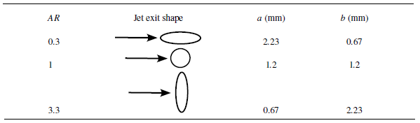


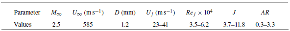
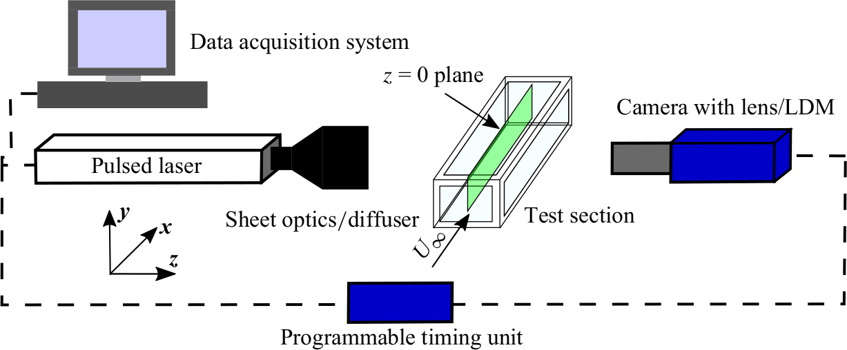

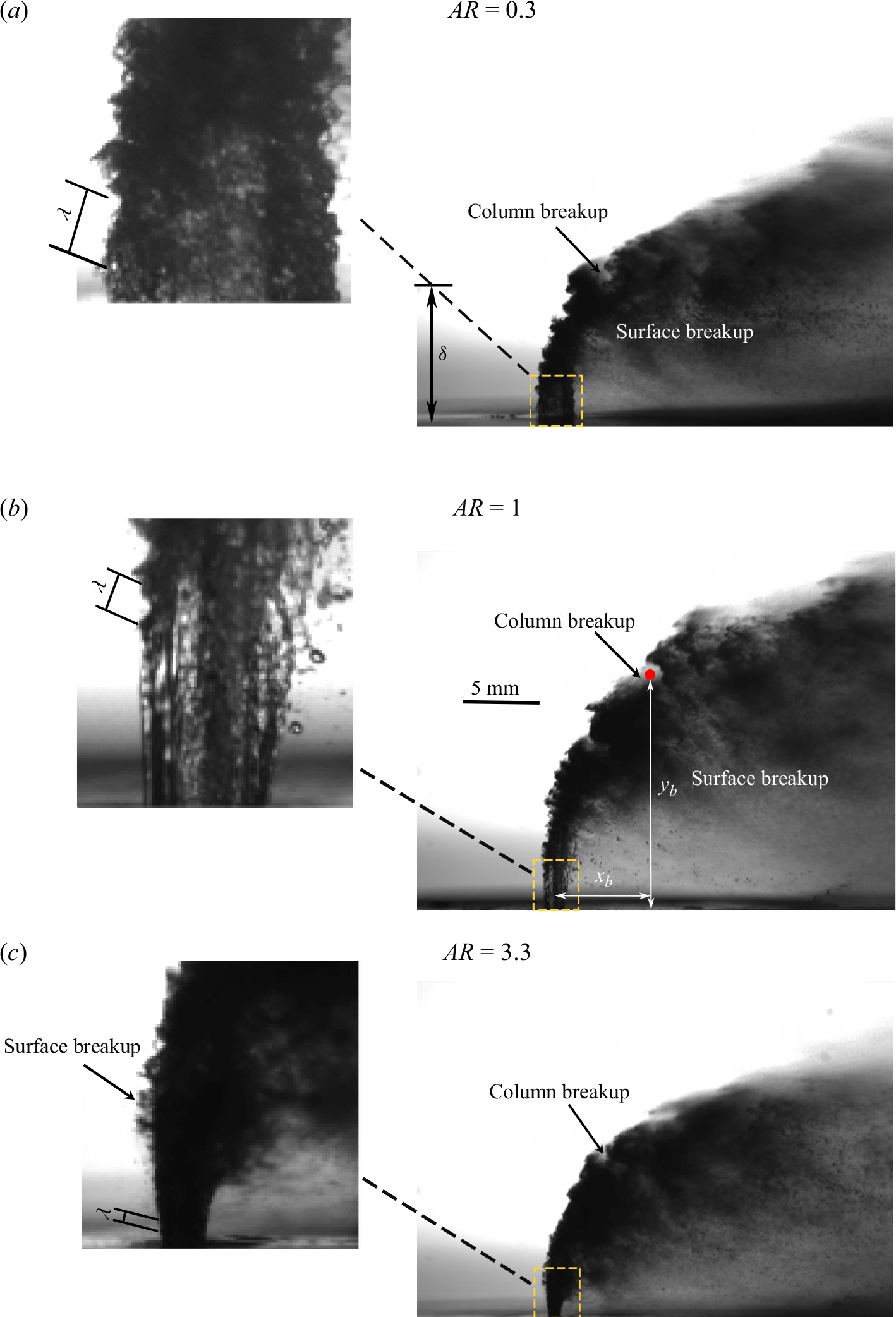


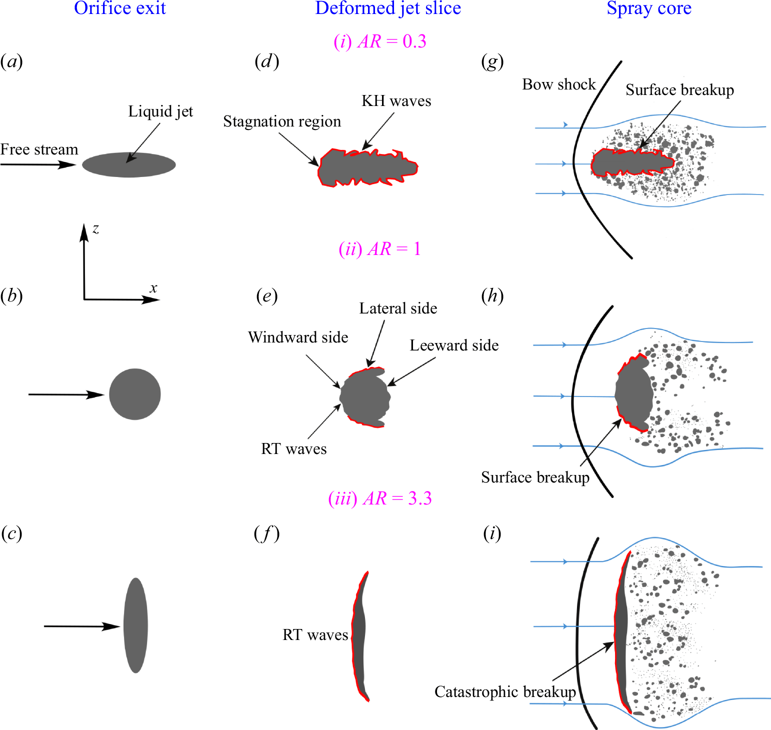
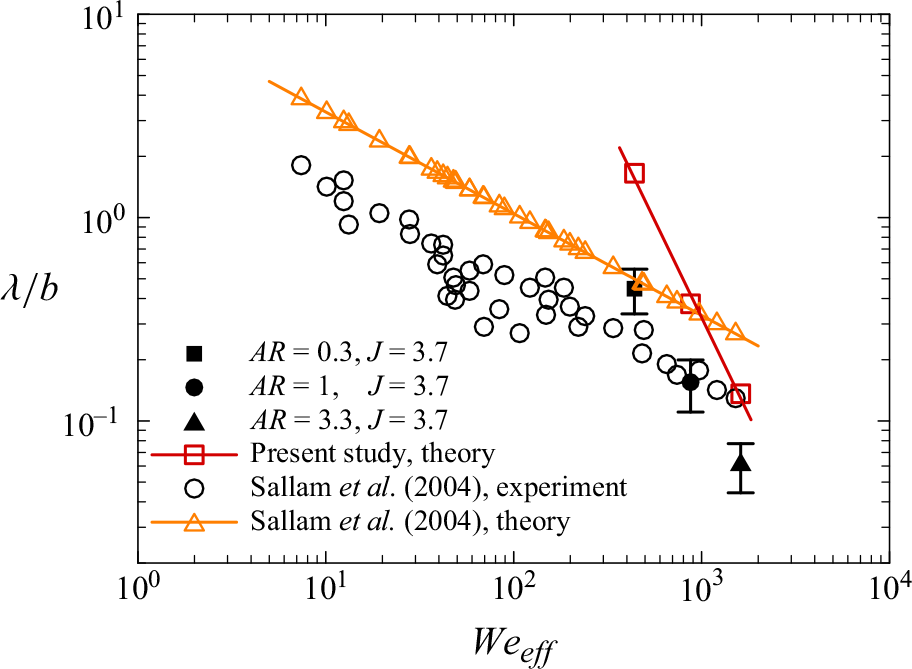


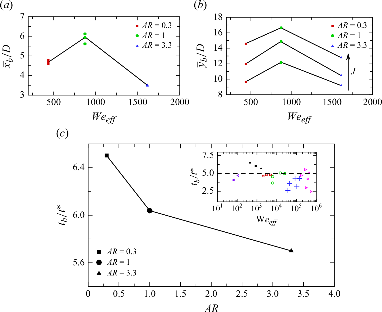


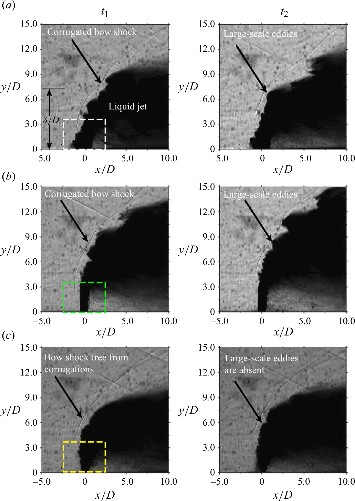


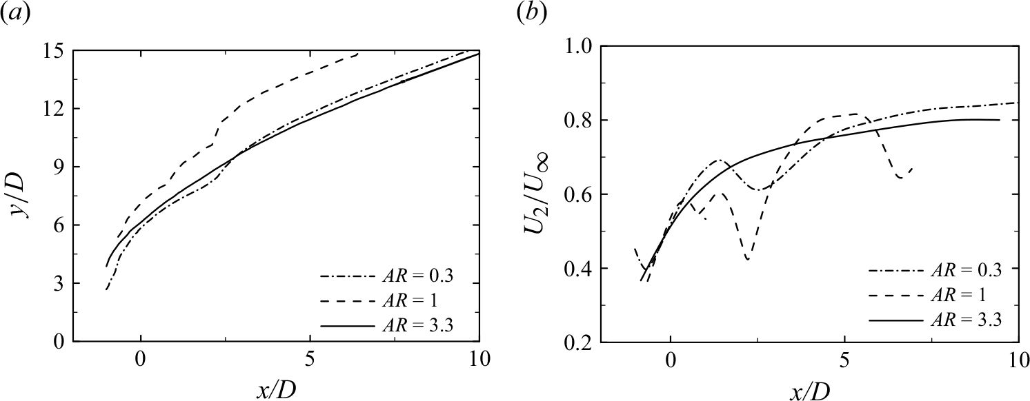


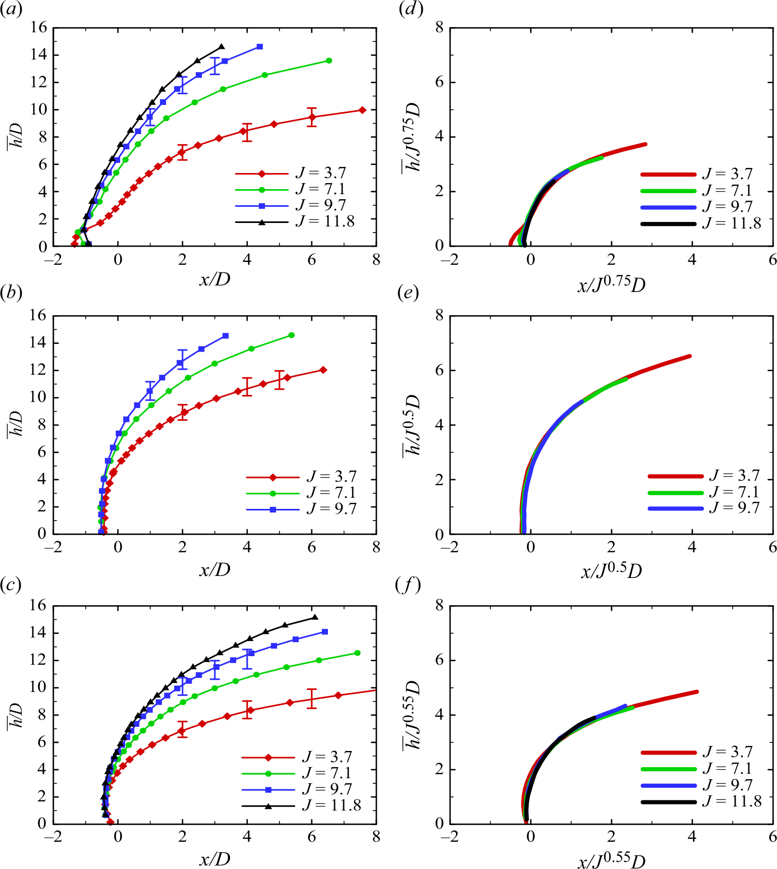


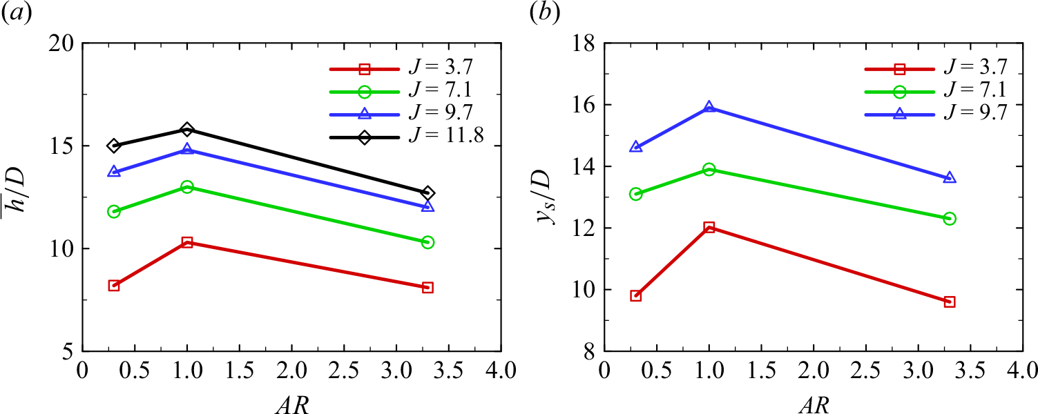


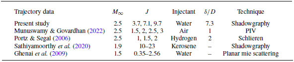
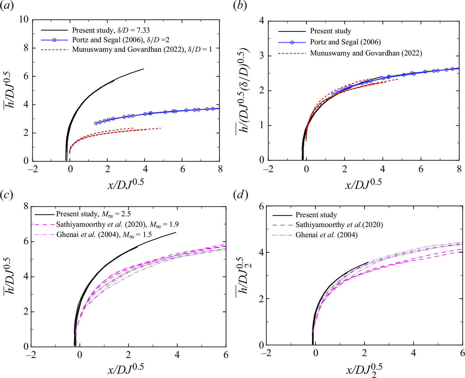


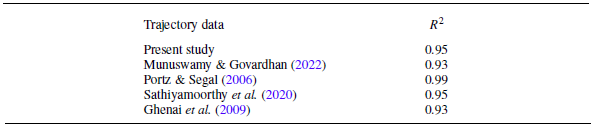


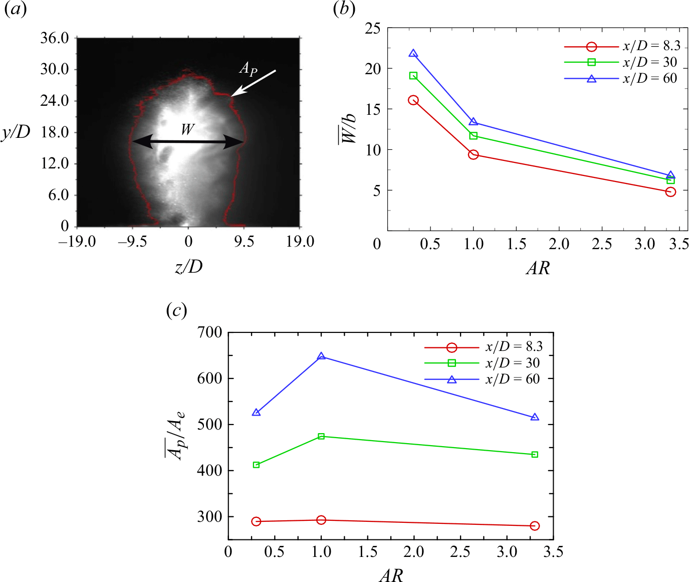


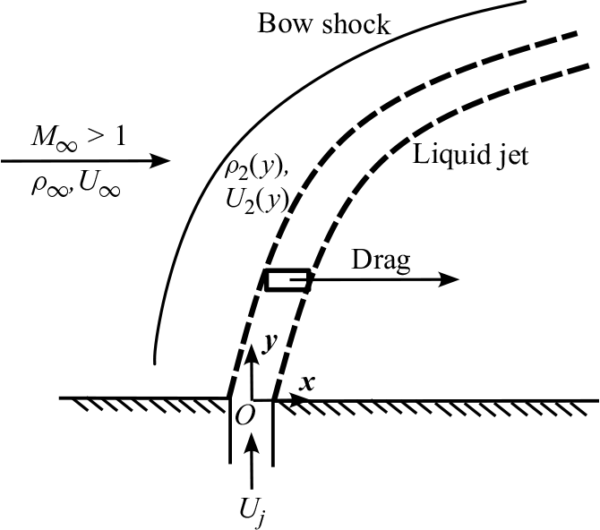

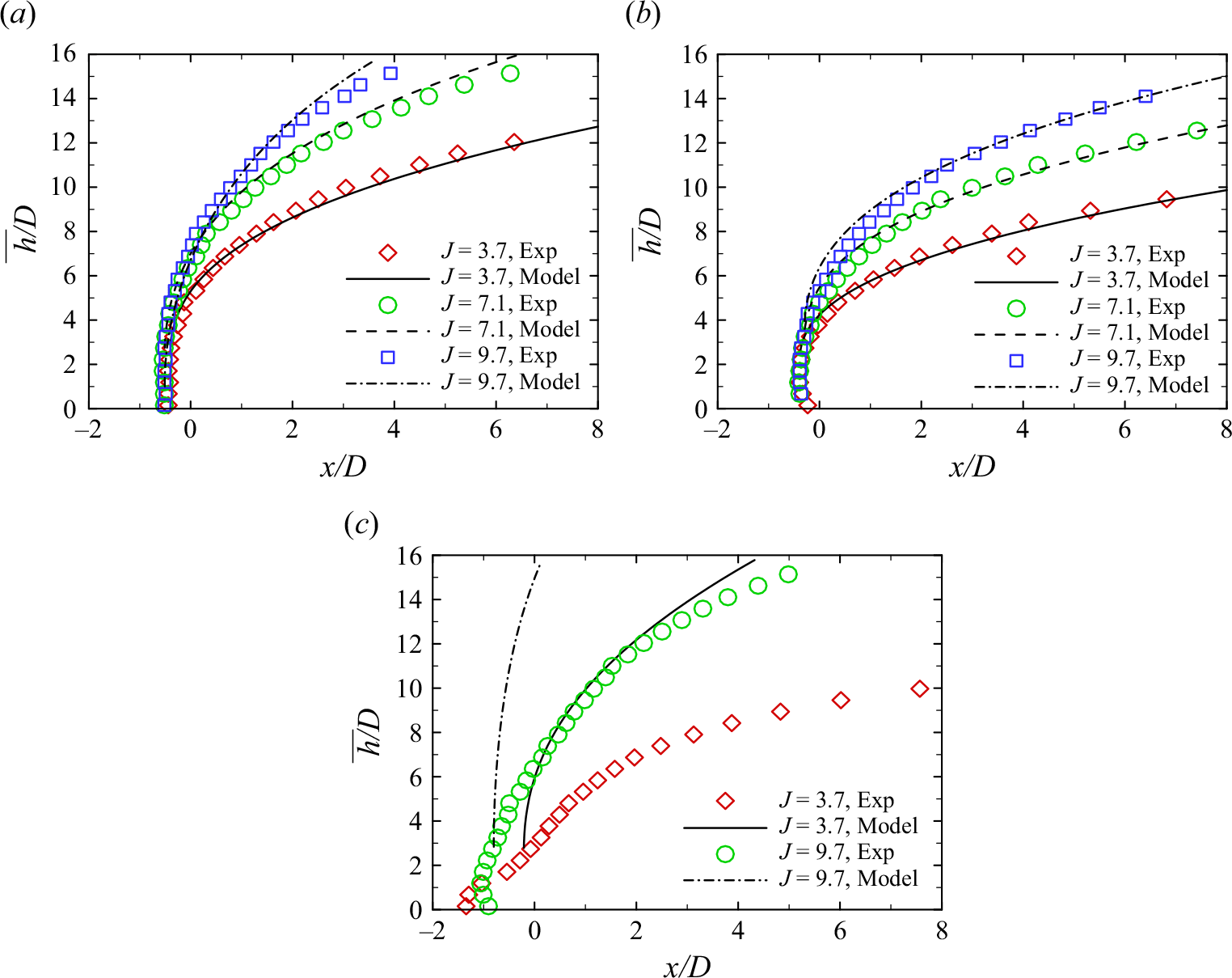


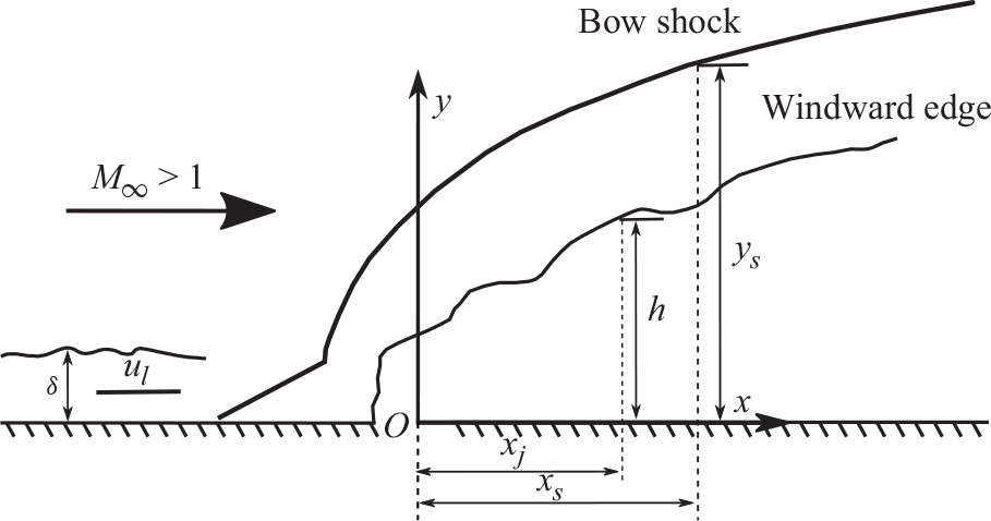


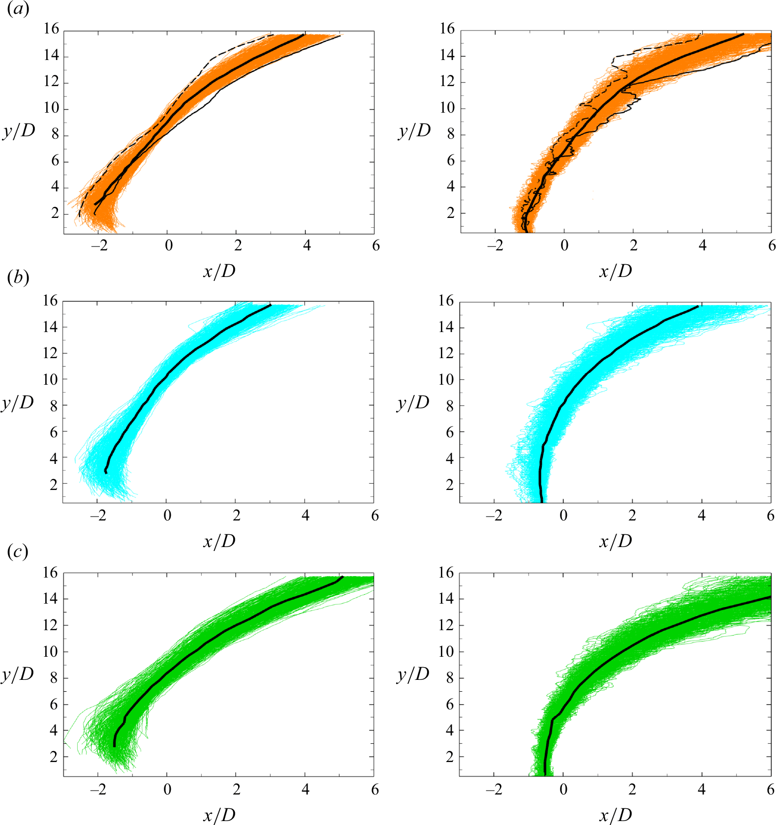


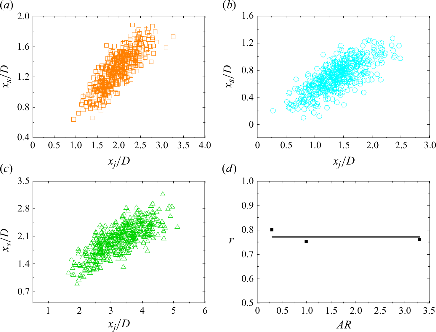


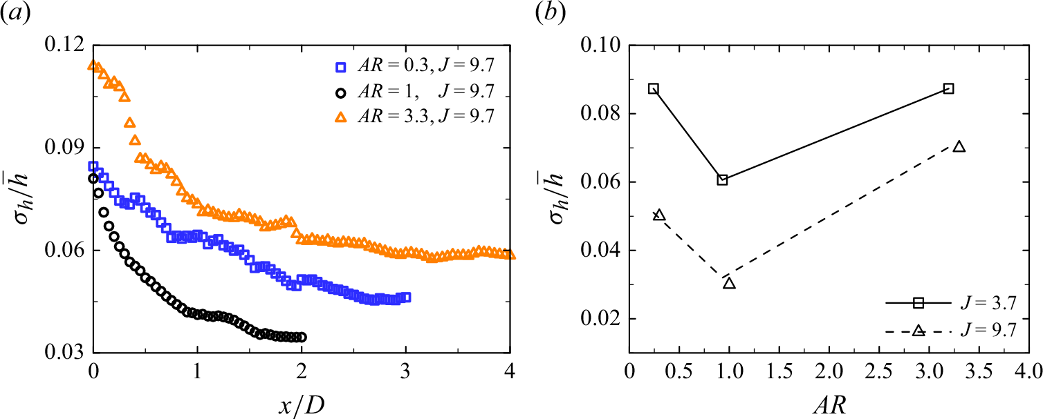


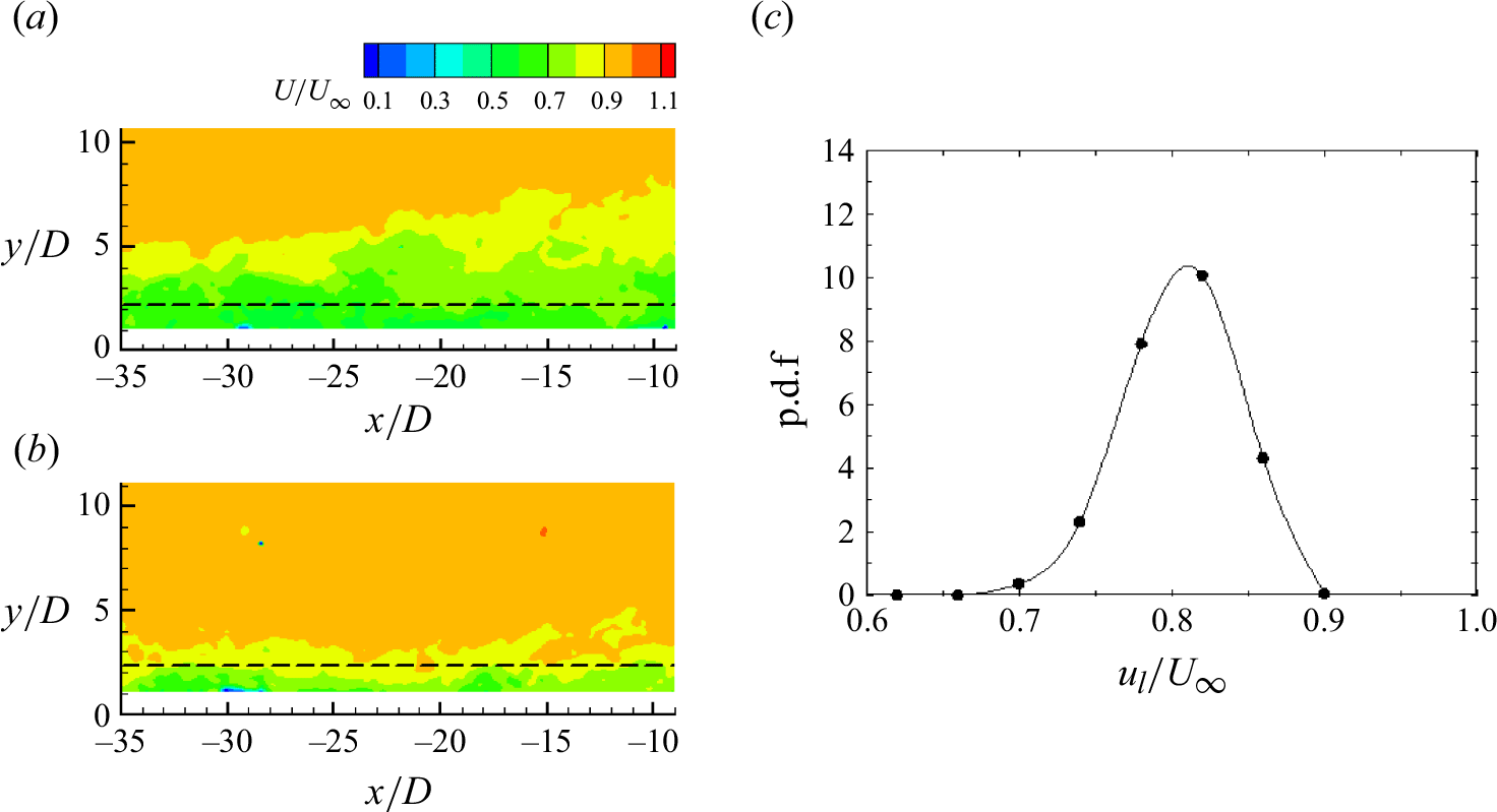


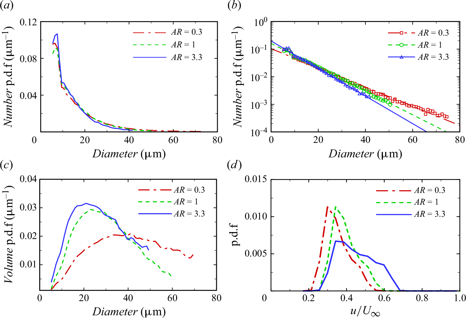


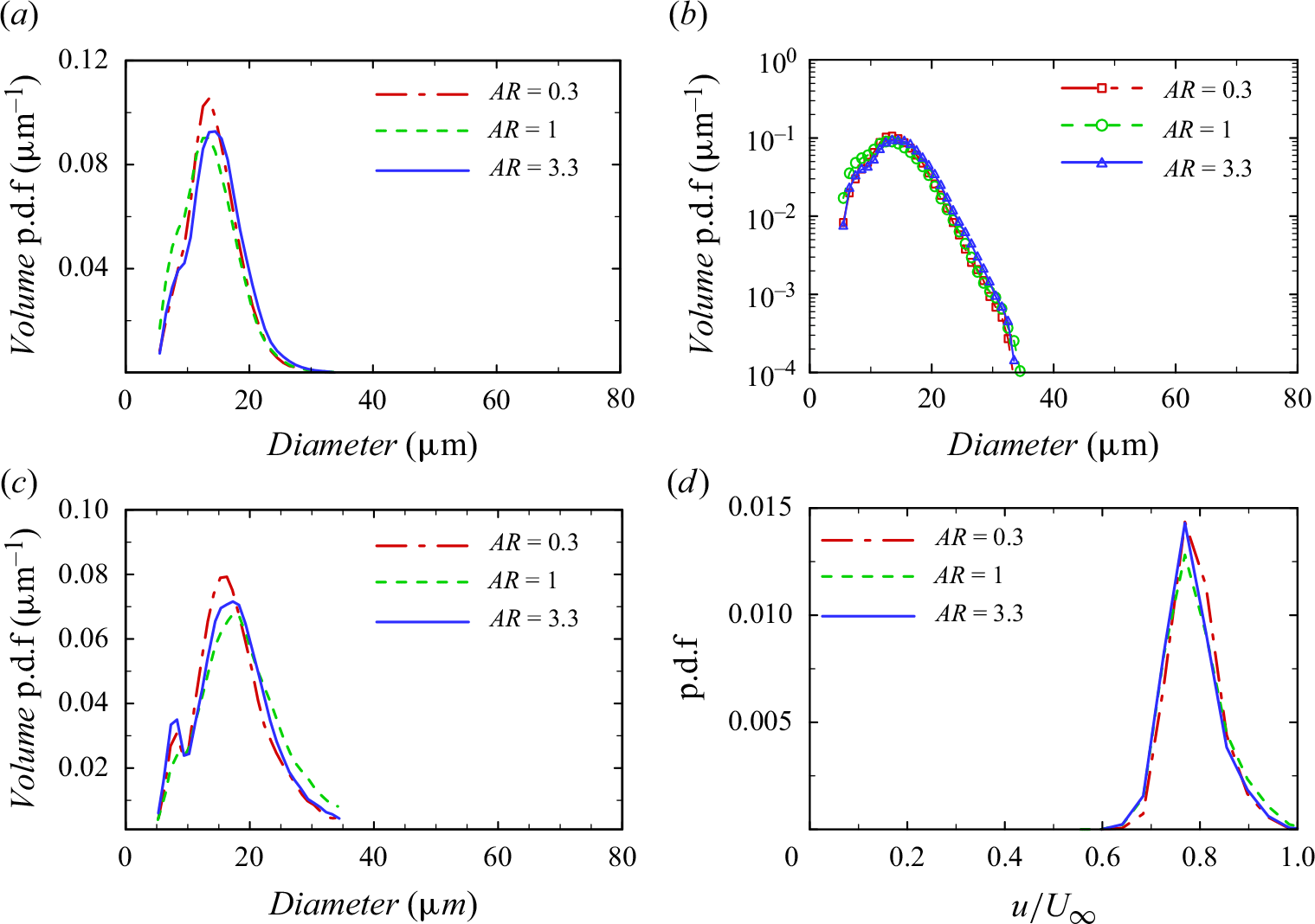


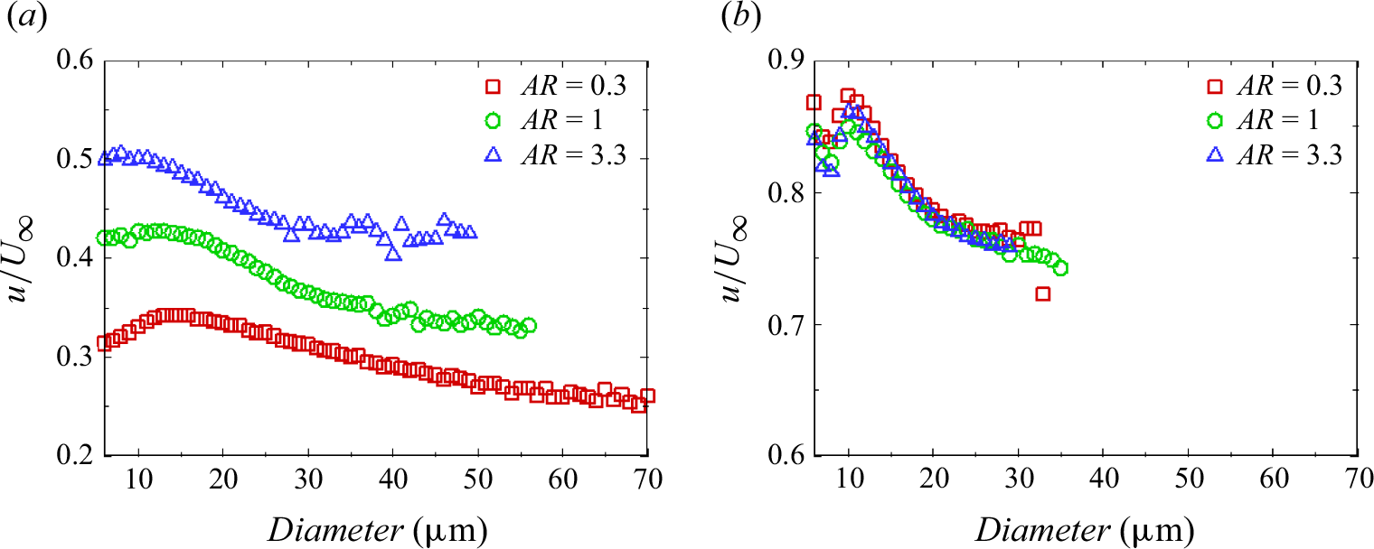


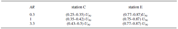

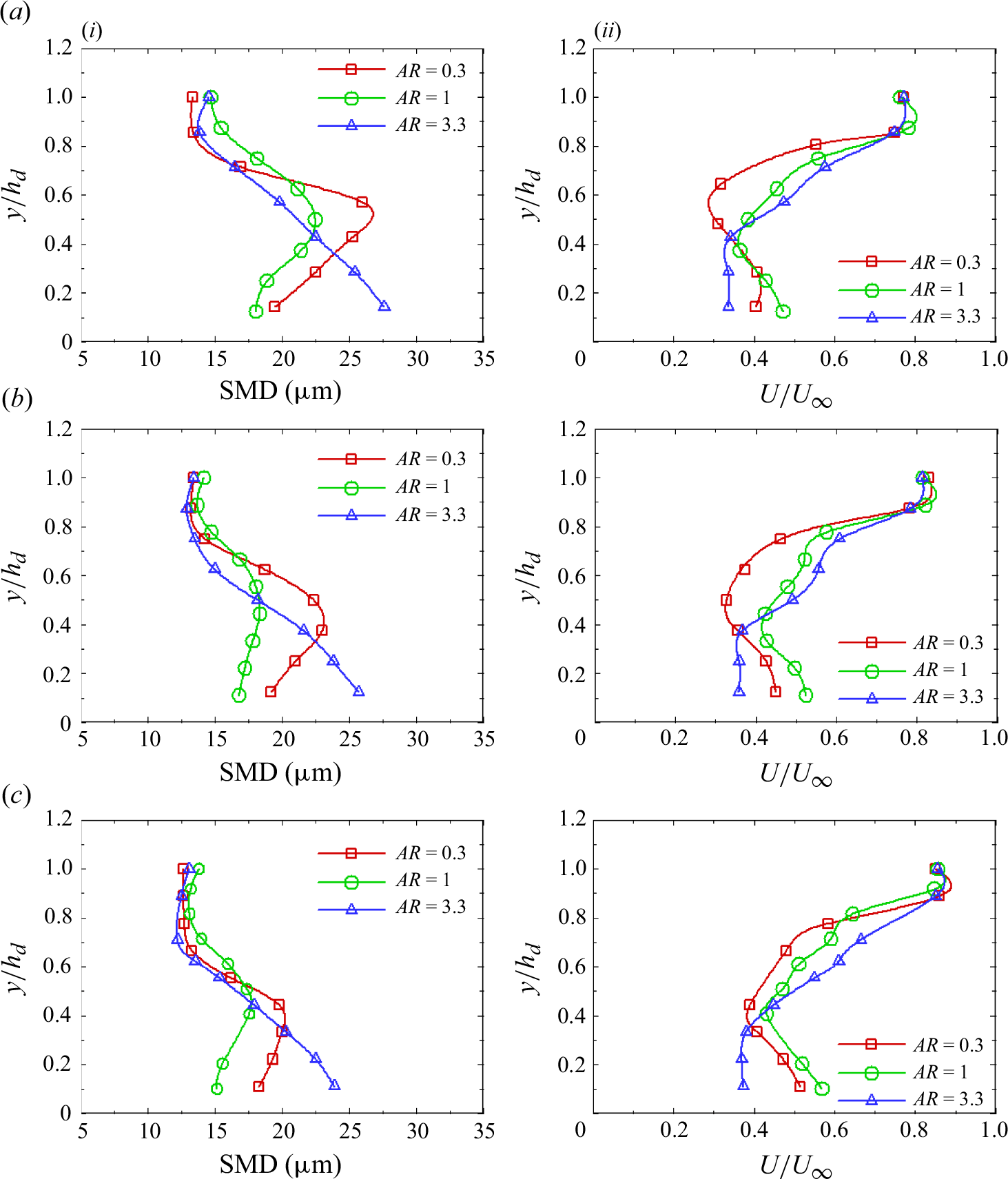


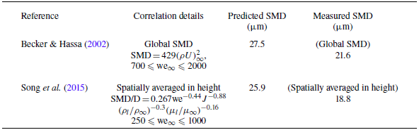


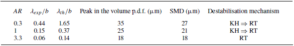

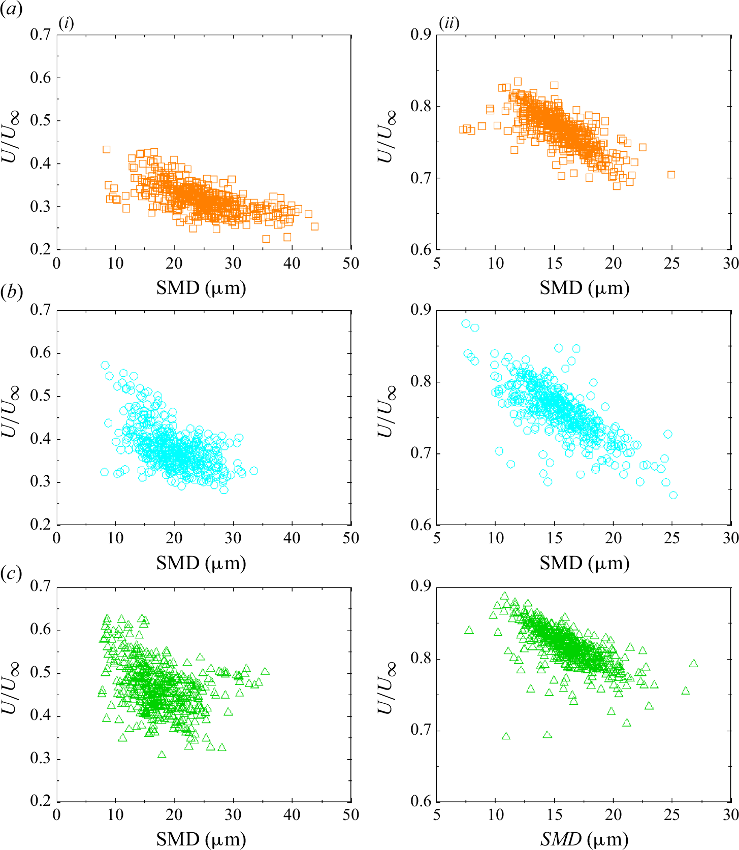


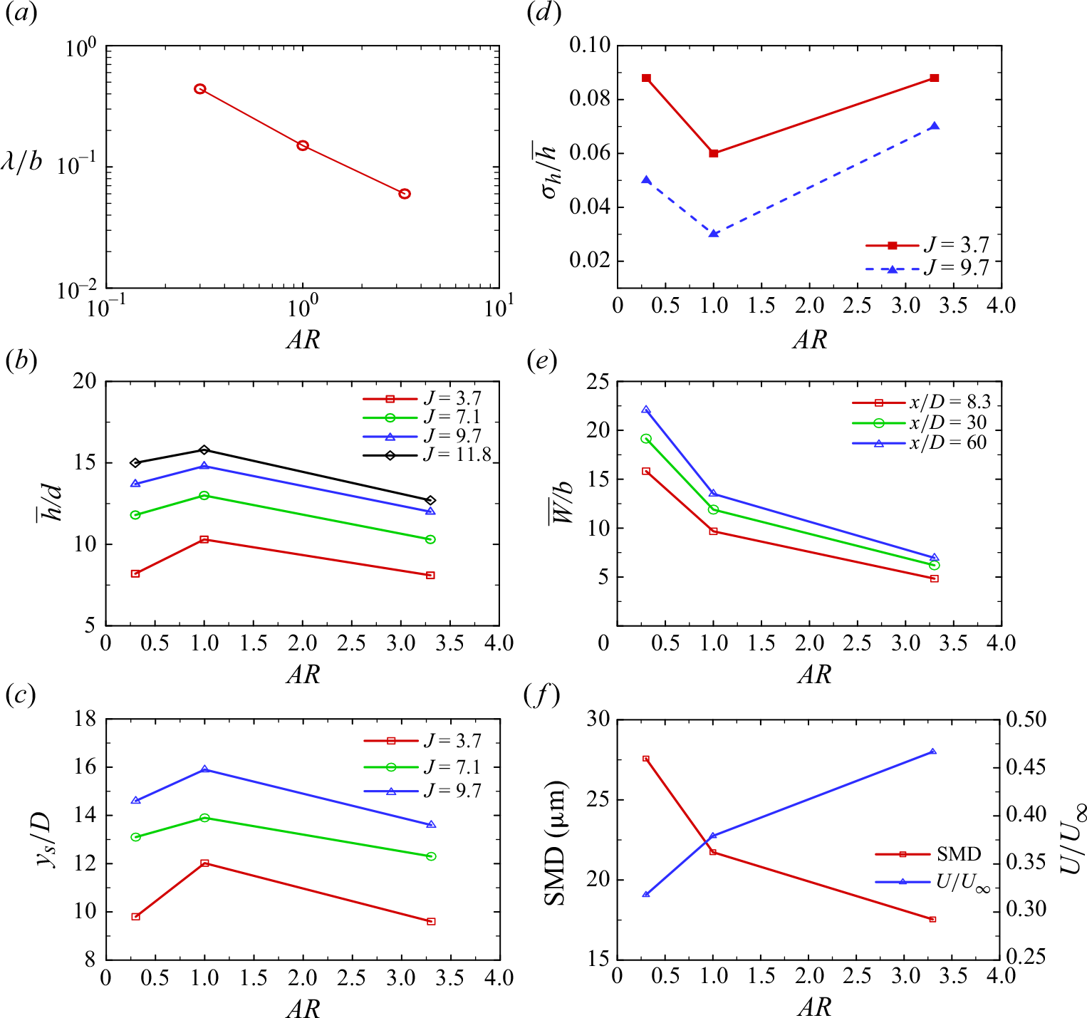


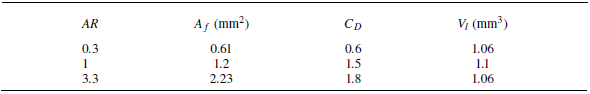


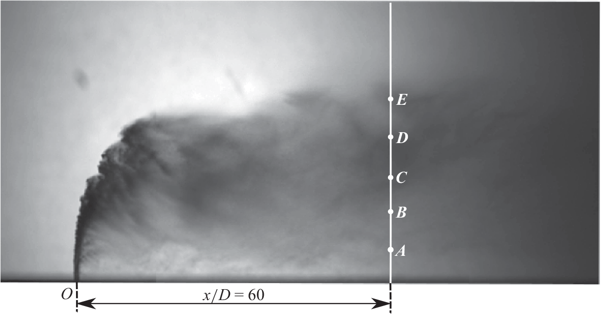


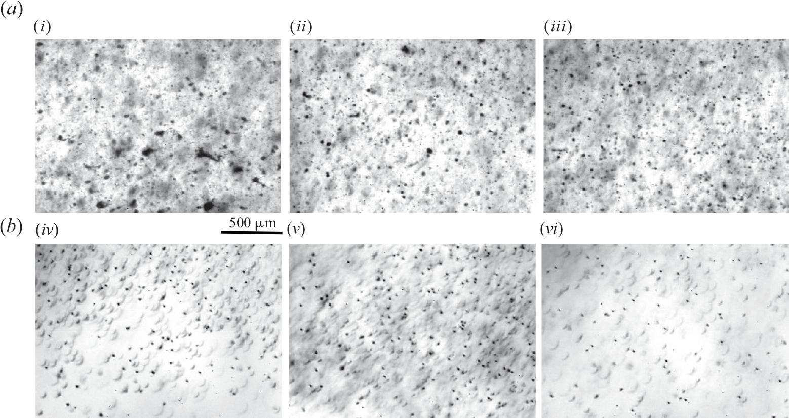


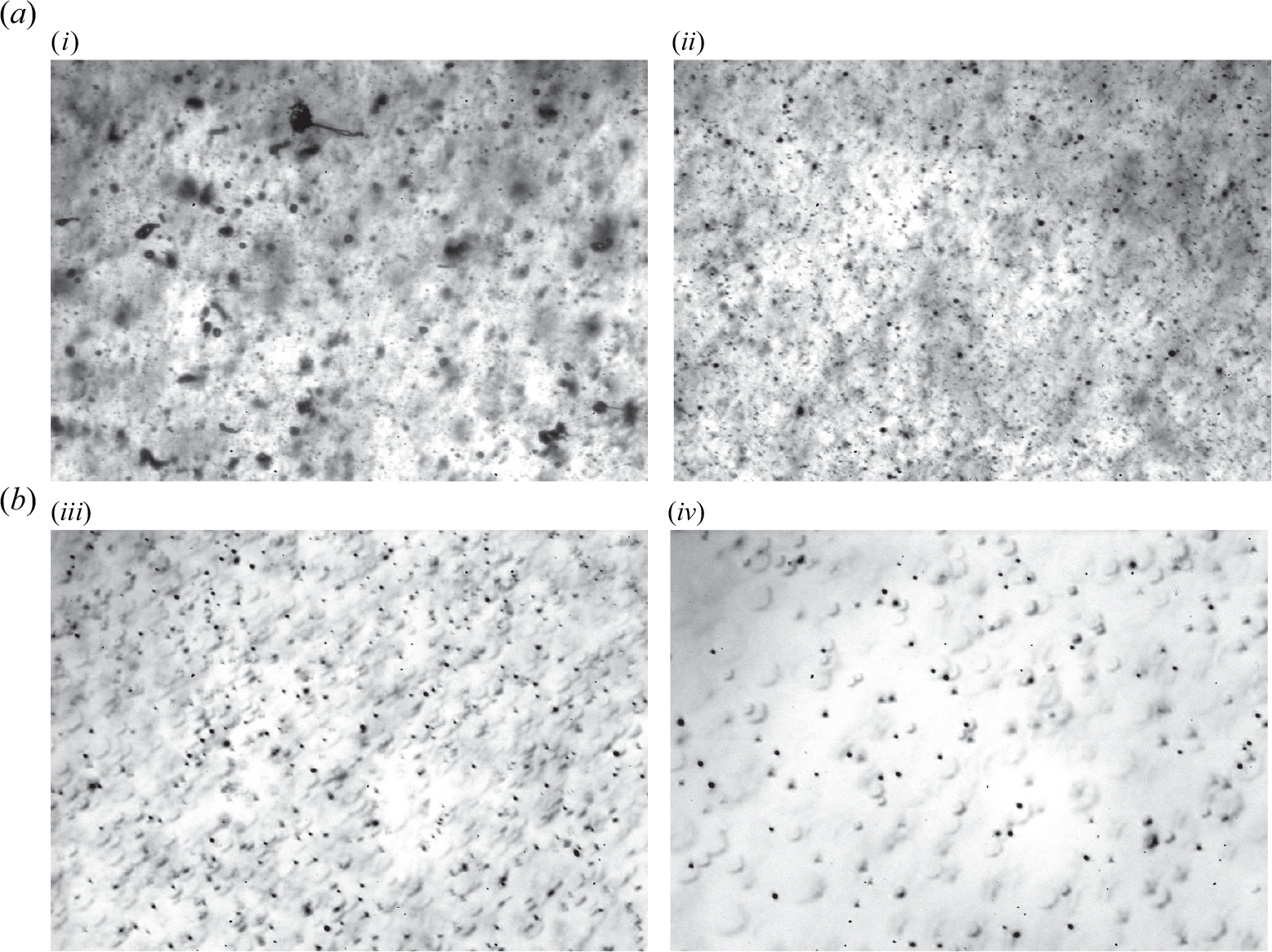


 Open access