


1. Introduction
Vertical natural convection boundary layers (NCBLs) are one of the most common configurations for buoyancy-driven flow and arise in a wide range of geophysical and engineering systems. Unlike the classical Rayleigh–Bénard convection (RBC), where the buoyancy force acts normal to the heated surface, vertical NCBLs are driven by buoyancy aligned parallel to the wall, leading to the development of a spatially developing boundary layer with mean shear.
A central parameter governing the dynamics of buoyancy-driven flows is the Prandtl number ( $ \textit{Pr}$
). While many studies have explored the flow mechanisms for vertical natural convection at individual Prandtl numbers, often air (
$ \textit{Pr}$
). While many studies have explored the flow mechanisms for vertical natural convection at individual Prandtl numbers, often air ( $ \textit{Pr} \approx 0.7$
, e.g. Tsuji & Nagano Reference Tsuji and Nagano1988; Nakao, Hattori & Suto Reference Nakao, Hattori and Suto2017) and water (
$ \textit{Pr} \approx 0.7$
, e.g. Tsuji & Nagano Reference Tsuji and Nagano1988; Nakao, Hattori & Suto Reference Nakao, Hattori and Suto2017) and water ( $ \textit{Pr} \approx 4{-} 7$
, e.g. Abedin, Tsuji & Hattori Reference Abedin, Tsuji and Hattori2009; Kogawa et al. Reference Kogawa, Okajima, Komiya, Armfield and Maruyama2016), there remains a lack of systematic investigations directly comparing flows across different Prandtl numbers under matched configurations to isolate and quantify the influence of Prandtl number. Carey & Mollendorf (Reference Carey and Mollendorf1978) experimentally investigated laminar natural convection along a vertical isoflux surface over a wide range of Prandtl numbers
$ \textit{Pr} \approx 4{-} 7$
, e.g. Abedin, Tsuji & Hattori Reference Abedin, Tsuji and Hattori2009; Kogawa et al. Reference Kogawa, Okajima, Komiya, Armfield and Maruyama2016), there remains a lack of systematic investigations directly comparing flows across different Prandtl numbers under matched configurations to isolate and quantify the influence of Prandtl number. Carey & Mollendorf (Reference Carey and Mollendorf1978) experimentally investigated laminar natural convection along a vertical isoflux surface over a wide range of Prandtl numbers $ (0.703\leqslant Pr \leqslant 8940 )$
and found good agreement with the similarity solution of Sparrow & Gregg (Reference Sparrow and Gregg1956) for low to moderate Prandtl numbers. However, at higher Prandtl number, their measured boundary layer becomes progressively thinner and deviates from the similarity prediction. Similar effects were also seen by Wickern (Reference Wickern1991), who investigated the laminar mixed convection along an arbitrarily inclined semi-infinite plate using low- and high-
$ (0.703\leqslant Pr \leqslant 8940 )$
and found good agreement with the similarity solution of Sparrow & Gregg (Reference Sparrow and Gregg1956) for low to moderate Prandtl numbers. However, at higher Prandtl number, their measured boundary layer becomes progressively thinner and deviates from the similarity prediction. Similar effects were also seen by Wickern (Reference Wickern1991), who investigated the laminar mixed convection along an arbitrarily inclined semi-infinite plate using low- and high- $ \textit{Pr}$
asymptotic expansions together with numerical solutions at finite Prandtl numbers (
$ \textit{Pr}$
asymptotic expansions together with numerical solutions at finite Prandtl numbers ( $0.02\leqslant \textit{Pr} \leqslant 50$
). Their analysis reveal that, in vertical configuration, the local heat transfer and the thicknesses of the velocity and temperature boundary layers inherit a strong
$0.02\leqslant \textit{Pr} \leqslant 50$
). Their analysis reveal that, in vertical configuration, the local heat transfer and the thicknesses of the velocity and temperature boundary layers inherit a strong $ \textit{Pr}$
dependence in both aiding and opposing cases, with the larger Prandtl number confining the buoyancy force to an increasingly thin near-wall region. Shapiro & Fedorovich (Reference Shapiro and Fedorovich2004) examined an unsteady laminar NCBL along an infinite vertical plate embedded in a stably stratified fluid with Prandtl numbers close to unity. Their numerical results for
$ \textit{Pr}$
dependence in both aiding and opposing cases, with the larger Prandtl number confining the buoyancy force to an increasingly thin near-wall region. Shapiro & Fedorovich (Reference Shapiro and Fedorovich2004) examined an unsteady laminar NCBL along an infinite vertical plate embedded in a stably stratified fluid with Prandtl numbers close to unity. Their numerical results for $0.5\leqslant \textit{Pr} \leqslant 1.5$
suggests that decreasing
$0.5\leqslant \textit{Pr} \leqslant 1.5$
suggests that decreasing $ \textit{Pr}$
produces thicker boundary layers that are more responsive to perturbations with stronger coupling between the thermal and velocity fields; whereas increasing
$ \textit{Pr}$
produces thicker boundary layers that are more responsive to perturbations with stronger coupling between the thermal and velocity fields; whereas increasing $ \textit{Pr}$
sharpens the near-wall gradients and the thermal layer, thereby modifying the transient growth of the momentum layer.
$ \textit{Pr}$
sharpens the near-wall gradients and the thermal layer, thereby modifying the transient growth of the momentum layer.
Such Prandtl number effects are shown to extend beyond the laminar regime. Linear stability analyses of the vertical NCBL reveal that the dominant instability mechanism shifts with Prandtl number (Hiebert & Gebhart Reference Hiebert and Gebhart1971; Janssen & Henkes Reference Janssen and Henkes1995; Janssen & Armfield Reference Janssen and Armfield1996; Xin & Le Quéré Reference Xin and Le Quéré2001) and strongly influences the transition Rayleigh number (Bejan & Lage Reference Bejan and Lage1990). Beyond the transition regime, previous experiments and simulations indicate that $ \textit{Pr}$
continues to affect vertical convection in the turbulent regime, though the nature and extent of this influence are less settled. An early theoretical work of Kraichnan (Reference Kraichnan1962) in RBC suggests that both heat transfer (in terms of the Nusselt number) and the flow structure are sensitive to the Prandtl number across all regimes. Using the mixing-length framework, Kraichnan (Reference Kraichnan1962) incorporated distinct eddy diffusivities for momentum and heat, and developed scaling estimates indicating that the turbulent heat transfer (in Nusselt number) and momentum development (in Reynolds number) exhibit distinct asymptotic dependencies on
$ \textit{Pr}$
continues to affect vertical convection in the turbulent regime, though the nature and extent of this influence are less settled. An early theoretical work of Kraichnan (Reference Kraichnan1962) in RBC suggests that both heat transfer (in terms of the Nusselt number) and the flow structure are sensitive to the Prandtl number across all regimes. Using the mixing-length framework, Kraichnan (Reference Kraichnan1962) incorporated distinct eddy diffusivities for momentum and heat, and developed scaling estimates indicating that the turbulent heat transfer (in Nusselt number) and momentum development (in Reynolds number) exhibit distinct asymptotic dependencies on $ \textit{Pr}$
. Based on their analysis, Kraichnan (Reference Kraichnan1962) further suggested this Prandtl number influence is more prominant for large Rayleigh number as the flow becomes more turbulent. These insights, while derived for RBC, have been widely extended to other buoyancy-driven flows, offering a conceptual framework for Prandtl-dependent scaling analyses (e.g. Ng et al. Reference Ng, Ooi, Lohse and Chung2018; Howland et al. Reference Howland, Ng, Verzicco and Lohse2022, in vertical NCBL). Recent experimental investigations have also demonstrated that variations in
$ \textit{Pr}$
. Based on their analysis, Kraichnan (Reference Kraichnan1962) further suggested this Prandtl number influence is more prominant for large Rayleigh number as the flow becomes more turbulent. These insights, while derived for RBC, have been widely extended to other buoyancy-driven flows, offering a conceptual framework for Prandtl-dependent scaling analyses (e.g. Ng et al. Reference Ng, Ooi, Lohse and Chung2018; Howland et al. Reference Howland, Ng, Verzicco and Lohse2022, in vertical NCBL). Recent experimental investigations have also demonstrated that variations in $ \textit{Pr}$
can significantly affect heat transfer in vertical convection systems, across a range of geometries and working fluids. Kang, Chung & Kim (Reference Kang, Chung and Kim2014) measured the heat transfer along a vertical heated cylinder in liquids with
$ \textit{Pr}$
can significantly affect heat transfer in vertical convection systems, across a range of geometries and working fluids. Kang, Chung & Kim (Reference Kang, Chung and Kim2014) measured the heat transfer along a vertical heated cylinder in liquids with $2094\leqslant \textit{Pr} \leqslant 5878$
. Their experimental results show that while laminar heat transfer closely follows the classical vertical flat plate correlations, turbulent heat transfer decreases with increasing
$2094\leqslant \textit{Pr} \leqslant 5878$
. Their experimental results show that while laminar heat transfer closely follows the classical vertical flat plate correlations, turbulent heat transfer decreases with increasing $ \textit{Pr}$
. Consistent with this trend, Chae & Chung (Reference Chae and Chung2015) conducted both experimental and numerical studies in a vertical rectangular chimney for
$ \textit{Pr}$
. Consistent with this trend, Chae & Chung (Reference Chae and Chung2015) conducted both experimental and numerical studies in a vertical rectangular chimney for $0.7\leqslant \textit{Pr} \leqslant 2094$
, where they found that the enhancement of heat transfer associated with the increased duct height diminishes at higher
$0.7\leqslant \textit{Pr} \leqslant 2094$
, where they found that the enhancement of heat transfer associated with the increased duct height diminishes at higher $ \textit{Pr}$
. More recently, Howland et al. (Reference Howland, Ng, Verzicco and Lohse2022) numerically investigated the vertical NCBL in a differentially heated channel for
$ \textit{Pr}$
. More recently, Howland et al. (Reference Howland, Ng, Verzicco and Lohse2022) numerically investigated the vertical NCBL in a differentially heated channel for $1\leqslant \textit{Pr} \leqslant 100$
up to
$1\leqslant \textit{Pr} \leqslant 100$
up to ${{Ra}}_H = 10^9$
, where
${{Ra}}_H = 10^9$
, where ${{Ra}}_H$
is the Rayleigh number based on the channel width. Using their direct numerical simulation (DNS) data, Howland et al. (Reference Howland, Ng, Verzicco and Lohse2022) showed that while the heat flux scales linearly with friction velocity at all Prandtl numbers considered, the boundary layer thickness and its structure are significantly affected by the Prandtl number. Similar observations are also seen in RBC studies, in which the flows are shown to have clear signs of persistent
${{Ra}}_H$
is the Rayleigh number based on the channel width. Using their direct numerical simulation (DNS) data, Howland et al. (Reference Howland, Ng, Verzicco and Lohse2022) showed that while the heat flux scales linearly with friction velocity at all Prandtl numbers considered, the boundary layer thickness and its structure are significantly affected by the Prandtl number. Similar observations are also seen in RBC studies, in which the flows are shown to have clear signs of persistent $ \textit{Pr}$
dependence in the thermal and velocity boundary layers in the turbulent regime (Belmonte, Tilgner & Libchaber Reference Belmonte, Tilgner and Libchaber1994; Xia & Zhou Reference Xia and Zhou2000; Pandey Reference Pandey2021). Consequently, although this Prandtl number dependence is clearly evident in both experimental and numerical literature, especially in the turbulent regime, its precise influence remains unresolved, particularly in the near-wall region, raising the question of whether separate scaling laws or corrections are needed to describe critical flow features across varying
$ \textit{Pr}$
dependence in the thermal and velocity boundary layers in the turbulent regime (Belmonte, Tilgner & Libchaber Reference Belmonte, Tilgner and Libchaber1994; Xia & Zhou Reference Xia and Zhou2000; Pandey Reference Pandey2021). Consequently, although this Prandtl number dependence is clearly evident in both experimental and numerical literature, especially in the turbulent regime, its precise influence remains unresolved, particularly in the near-wall region, raising the question of whether separate scaling laws or corrections are needed to describe critical flow features across varying $ \textit{Pr}$
.
$ \textit{Pr}$
.
In addition, more recent studies revealed a two-stage evolution of turbulence in the vertical NCBL (Wells & Worster Reference Wells and Worster2008; Ng et al. Reference Ng, Ooi, Lohse and Chung2015, Reference Ng, Ooi, Lohse and Chung2017; Ke et al. Reference Ke, Williamson, Armfield, Komiya and Norris2021, Reference Ke, Williamson, Armfield and Komiya2023; Wells Reference Wells2023): beyond the initial laminar–turbulent transition, the flow enters a classical weakly turbulent regime where turbulence is largely confined to the outer plume, while the near-wall region remains laminar-like. At higher Rayleigh numbers, the increasing near-wall shear triggers a second transition, giving rise to a fully turbulent boundary layer where both the near-wall and outer regions are turbulent. This regime, referred to as the ultimate turbulent regime, is consistent with the turbulence development in classical wall-bounded flows and RBC (Kraichnan Reference Kraichnan1962; Grossmann & Lohse Reference Grossmann and Lohse2000, Reference Grossmann and Lohse2011). These recent advances underscore the importance of shear–buoyancy interaction in governing the turbulent regime transitions. However, it remains unclear how Prandtl number influences near-wall turbulent structure across these regimes.
The present study investigates the influence of Prandtl number on the development of vertical NCBL. Direct numerical simulations are performed for $ \textit{Pr} =4.16$
(corresponding to water at
$ \textit{Pr} =4.16$
(corresponding to water at $315\,\rm K$
) and
$315\,\rm K$
) and $ \textit{Pr} =6$
(corresponding to water at
$ \textit{Pr} =6$
(corresponding to water at $298\,\rm K$
) in a temporally developing configuration, in which periodic boundary conditions are applied in the streamwise direction to ensure a spatially invariant flow. This temporal framework has been applied to a number of flows that are generally thought spatially developing (e.g. Kozul, Chung & Monty Reference Kozul, Chung and Monty2016; Abedin et al. Reference Abedin, Tsuji and Hattori2009, Reference Abedin, Tsuji and Hattori2010), with a greatly reduced computational domain size and grid resolution. The results are analysed together with the DNS dataset for
$298\,\rm K$
) in a temporally developing configuration, in which periodic boundary conditions are applied in the streamwise direction to ensure a spatially invariant flow. This temporal framework has been applied to a number of flows that are generally thought spatially developing (e.g. Kozul, Chung & Monty Reference Kozul, Chung and Monty2016; Abedin et al. Reference Abedin, Tsuji and Hattori2009, Reference Abedin, Tsuji and Hattori2010), with a greatly reduced computational domain size and grid resolution. The results are analysed together with the DNS dataset for $ \textit{Pr} =0.71$
previously reported by Ke et al. (Reference Ke, Williamson, Armfield and Komiya2023), enabling a direct statistical comparison across Prandtl numbers. The remainder of the paper is organised as follows. Section 2 provides an overview and the mathematical description of the problem. In § 3.1, the mean velocity and temperature profiles are compared across different Prandtl numbers. Section 3.2 introduces a thermal Rayleigh number based on the thermal boundary layer thickness, with which our DNS data show good collapse in the Nusselt number scaling across Prandtl numbers and flow regimes. Sections 3.3 and 3.4 further analyse the momentum field development using skin friction scaling and premultiplied spectra to examine the Prandtl number dependence of the onset of the ultimate regime and its associated near-wall streak structures. Section 4 briefly concludes the findings in this paper.
$ \textit{Pr} =0.71$
previously reported by Ke et al. (Reference Ke, Williamson, Armfield and Komiya2023), enabling a direct statistical comparison across Prandtl numbers. The remainder of the paper is organised as follows. Section 2 provides an overview and the mathematical description of the problem. In § 3.1, the mean velocity and temperature profiles are compared across different Prandtl numbers. Section 3.2 introduces a thermal Rayleigh number based on the thermal boundary layer thickness, with which our DNS data show good collapse in the Nusselt number scaling across Prandtl numbers and flow regimes. Sections 3.3 and 3.4 further analyse the momentum field development using skin friction scaling and premultiplied spectra to examine the Prandtl number dependence of the onset of the ultimate regime and its associated near-wall streak structures. Section 4 briefly concludes the findings in this paper.
2. Problem definition and numerical method
2.1. Mathematical description
The problem under consideration is a natural convection flow along an isothermally heated vertical wall of infinite extent. The fluid motion is governed by the conservation equations of mass, momentum and energy, which, under the assumptions of incompressibility and the Oberbeck–Boussinesq approximation, are given in dimensional form by
 \begin{align} \frac {\partial \hat {u_i}}{\partial {x_i}}& = 0, \end{align}
 \begin{align} \frac {\partial \hat {u_i}}{\partial {t}}+\frac {\partial \hat {u_i} \hat {u_j}}{\partial {x_j}} & = -\frac {1}{{\rho }}\frac {\partial \hat {p}}{\partial {x_i}}+{\nu }\frac {\partial ^2 \hat {u_i}}{\partial {x_j}^2}+ {g}{\beta }\big (\hat {T}-\hat {T}_\infty \big )\delta _{i1},\end{align}
 \begin{align} \frac {\partial \hat {T}}{\partial {t}}+\frac {\partial \hat {u_j} \hat {T}}{\partial {x_j}} & ={\kappa }\frac {\partial ^2 \hat {T}}{\partial {x_j}^2},\end{align}
where $\hat {u}$
and
$\hat {u}$
and $\hat {p}$
denote the dimensional velocity field and pressure field, respectively; and
$\hat {p}$
denote the dimensional velocity field and pressure field, respectively; and $\hat {T}$
represents the dimensional temperature field. The subscripts
$\hat {T}$
represents the dimensional temperature field. The subscripts $i, j = 1, 2, 3$
denote the
$i, j = 1, 2, 3$
denote the $x$
(streamwise),
$x$
(streamwise), $y$
(wall-normal) and
$y$
(wall-normal) and $z$
(spanwise) directions, respectively; and
$z$
(spanwise) directions, respectively; and $\delta _{i1}$
is the Kronecker delta, which indicates that the buoyancy force acts only in the
$\delta _{i1}$
is the Kronecker delta, which indicates that the buoyancy force acts only in the $x$
direction. In (2.1), we also specify
$x$
direction. In (2.1), we also specify $\beta$
as the thermal expansion coefficient,
$\beta$
as the thermal expansion coefficient, $g$
as the gravitational acceleration,
$g$
as the gravitational acceleration, $\nu$
as the viscosity and
$\nu$
as the viscosity and $\kappa$
as the thermal diffusivity of the working fluid – the ratio of which defines the Prandtl number,
$\kappa$
as the thermal diffusivity of the working fluid – the ratio of which defines the Prandtl number,
 \begin{equation} \textit{Pr} \equiv \frac {\nu }{\kappa }. \end{equation}
In the sections that follow, all results and analyses are reported in dimensionless form. The temperature field is made dimensionless with $\theta = (\hat {T}-\hat {T}_\infty )/\Delta \hat {T}$
, where
$\theta = (\hat {T}-\hat {T}_\infty )/\Delta \hat {T}$
, where $\Delta \hat {T} = \hat {T}_w - \hat {T}_\infty$
is the bulk temperature difference between the isothermal wall
$\Delta \hat {T} = \hat {T}_w - \hat {T}_\infty$
is the bulk temperature difference between the isothermal wall $\hat {T}_w$
and the ambient
$\hat {T}_w$
and the ambient $\hat {T}_\infty$
. For a doubly infinite free convection flow, the velocity fields are made dimensionless using the intrinsic velocity scale
$\hat {T}_\infty$
. For a doubly infinite free convection flow, the velocity fields are made dimensionless using the intrinsic velocity scale $U_s = (g\beta \kappa \Delta \hat {T} )^{1/3}$
such that the dimensionless velocity is given by
$U_s = (g\beta \kappa \Delta \hat {T} )^{1/3}$
such that the dimensionless velocity is given by $u_i = \hat {u_i}/U_s$
. Since there is no inherent natural length scale in this temporally evolving configuration, we adopt the intrinsic length scale
$u_i = \hat {u_i}/U_s$
. Since there is no inherent natural length scale in this temporally evolving configuration, we adopt the intrinsic length scale $L_s= \kappa ^{2/3}/ (g\beta \Delta \hat {T} )^{1/3}$
for non-dimensionalisation.
$L_s= \kappa ^{2/3}/ (g\beta \Delta \hat {T} )^{1/3}$
for non-dimensionalisation.
The fluid flow system (2.1) has an analytical laminar solution (Illingworth Reference Illingworth1950; Schetz & Eichhorn Reference Schetz and Eichhorn1962) – for $ \textit{Pr} \neq 1$
, the dimensionless temperature and streamwise velocity follows
$ \textit{Pr} \neq 1$
, the dimensionless temperature and streamwise velocity follows
 \begin{align} \theta & = \theta _w{\text{erfc}}\left (\eta \right ), \end{align}
 \begin{align} u & = \frac {4\theta _w t}{1- \textit{Pr} }\left [{\mathrm{i^2 erfc}}(\eta )-{\mathrm{i^2 erfc}}\left (\frac {\eta }{\sqrt { \textit{Pr} }}\right )\right ]\!,\end{align}
where $\eta =y/\sqrt {4\kappa t}$
is the similarity coordinate and i
$\eta =y/\sqrt {4\kappa t}$
is the similarity coordinate and i $^n$
erfc
$^n$
erfc $(\eta )$
is the
$(\eta )$
is the $n$
th integral of the complementary error function
$n$
th integral of the complementary error function ${\text{erfc}}(\eta )$
. Equation (2.3) represents a temporally developing, one-dimensional solution in which the flow is streamwise and spanwise invariant, and both the temperature and velocity fields depend solely on the wall-normal distance
${\text{erfc}}(\eta )$
. Equation (2.3) represents a temporally developing, one-dimensional solution in which the flow is streamwise and spanwise invariant, and both the temperature and velocity fields depend solely on the wall-normal distance $y$
and time
$y$
and time $t$
through the similarity parameter
$t$
through the similarity parameter $\eta$
. As a result, the streamwise extent
$\eta$
. As a result, the streamwise extent $x$
, which is typically used to characterise the local flow development in spatially developing configurations, is not applicable in the temporally developing case. In spatially developing flows (e.g. Tsuji & Nagano Reference Tsuji and Nagano1988; Tsuji & Kajitani Reference Tsuji and Kajitani2006; Nakao et al. Reference Nakao, Hattori and Suto2017), statistics are commonly obtained through time averaging since the flow is steady in the mean and develops in the downstream direction (
$x$
, which is typically used to characterise the local flow development in spatially developing configurations, is not applicable in the temporally developing case. In spatially developing flows (e.g. Tsuji & Nagano Reference Tsuji and Nagano1988; Tsuji & Kajitani Reference Tsuji and Kajitani2006; Nakao et al. Reference Nakao, Hattori and Suto2017), statistics are commonly obtained through time averaging since the flow is steady in the mean and develops in the downstream direction ( $x$
). In contrast, for the temporally developing NCBL, the parallel flow is unsteady in the mean and the instantaneous (local) statistics are obtained by averaging over the homogeneous
$x$
). In contrast, for the temporally developing NCBL, the parallel flow is unsteady in the mean and the instantaneous (local) statistics are obtained by averaging over the homogeneous $x$
–
$x$
– $z$
plane. Accordingly, the unsteady parallel flow at a given time is characterised by the instantaneous momentum boundary layer thickness
$z$
plane. Accordingly, the unsteady parallel flow at a given time is characterised by the instantaneous momentum boundary layer thickness $\delta (t)$
, which provides a natural length scale for defining the Grashof and Rayleigh numbers,
$\delta (t)$
, which provides a natural length scale for defining the Grashof and Rayleigh numbers,
 \begin{equation} {{Gr}}_\delta = \frac {g\beta \theta _w\delta ^3}{\nu ^2},\quad {{Ra}}_\delta = {{Gr}}_\delta \textit{Pr} ,\quad \delta =\int _0^\infty \frac {\bar {u}}{\overline {u}_m}\,\mathrm{d}y, \end{equation}
where $\bar {u}$
is the instantaneous mean streamwise velocity averaged over the homogeneous (
$\bar {u}$
is the instantaneous mean streamwise velocity averaged over the homogeneous ( $x$
–
$x$
– $z$
) plane and
$z$
) plane and $\overline {u}_m$
denotes the maximum value of the instantaneous mean
$\overline {u}_m$
denotes the maximum value of the instantaneous mean $\bar {u}$
. Notably, the resulting momentum boundary layer thickness, as well as the corresponding Grashof and Rayleigh number, are essentially functions of time only, i.e.
$\bar {u}$
. Notably, the resulting momentum boundary layer thickness, as well as the corresponding Grashof and Rayleigh number, are essentially functions of time only, i.e. $\delta (t)$
,
$\delta (t)$
, ${{Gr}}_\delta (t)$
and
${{Gr}}_\delta (t)$
and ${{Ra}}_\delta (t)$
. Similar definitions have been used in recent studies of temporally developing flows (e.g. Abedin et al. Reference Abedin, Tsuji and Hattori2009; Ke et al. Reference Ke, Williamson, Armfield, Norris and Komiya2020), where turbulence statistics are compared with those from spatially developing flows by matching the boundary layer thickness, showing excellent agreement.
${{Ra}}_\delta (t)$
. Similar definitions have been used in recent studies of temporally developing flows (e.g. Abedin et al. Reference Abedin, Tsuji and Hattori2009; Ke et al. Reference Ke, Williamson, Armfield, Norris and Komiya2020), where turbulence statistics are compared with those from spatially developing flows by matching the boundary layer thickness, showing excellent agreement.
2.2. Direct numerical simulation
In the present study, we conduct DNS at Prandtl numbers $ \textit{Pr} =4.16$
and
$ \textit{Pr} =4.16$
and $ \textit{Pr} =6$
, and analyse the dataset previously reported by Ke et al. (Reference Ke, Williamson, Armfield and Komiya2023) at
$ \textit{Pr} =6$
, and analyse the dataset previously reported by Ke et al. (Reference Ke, Williamson, Armfield and Komiya2023) at $ \textit{Pr} =0.71$
, thereby enabling a direct statistical comparison across Prandtl numbers. This Prandtl number range was chosen to represent fluids of broad practical relevance in engineering and geophysical applications. While extreme
$ \textit{Pr} =0.71$
, thereby enabling a direct statistical comparison across Prandtl numbers. This Prandtl number range was chosen to represent fluids of broad practical relevance in engineering and geophysical applications. While extreme $ \textit{Pr}$
regimes (e.g.
$ \textit{Pr}$
regimes (e.g. $ \textit{Pr} \ll 1$
, liquid metals;
$ \textit{Pr} \ll 1$
, liquid metals; $ \textit{Pr} \gg 10$
, highly viscous oils) are also of interest, DNS at these limits entails substantially increased computational cost due to disparate scales of motions and stricter resolution requirements, and a detailed exploration of such cases lies beyond the scope of the present study.
$ \textit{Pr} \gg 10$
, highly viscous oils) are also of interest, DNS at these limits entails substantially increased computational cost due to disparate scales of motions and stricter resolution requirements, and a detailed exploration of such cases lies beyond the scope of the present study.
The numerical set-up follows that of Ke et al. (Reference Ke, Williamson, Armfield, Komiya and Norris2021, Reference Ke, Williamson, Armfield and Komiya2023), in which a streamwise-invariant, temporally developing parallel flow is obtained by imposing periodic boundary conditions, as depicted in figure 1. A Cartesian finite volume grid is employed to discretise the computational domain, with uniform spacing in the homogeneous directions (streamwise and spanwise). In the wall-normal direction, a logarithmically stretched mesh is used up to half the domain width such that the $i$
th cell in this region is given by
$i$
th cell in this region is given by $\Delta y_i = \Delta y_{min }\,\gamma ^{\,i-1}$
, where
$\Delta y_i = \Delta y_{min }\,\gamma ^{\,i-1}$
, where $\Delta y_{min }$
is the first off-wall spacing and the stretching factor
$\Delta y_{min }$
is the first off-wall spacing and the stretching factor $\gamma$
is determined from
$\gamma$
is determined from $\Delta y_{min }(1-\gamma ^{N})/(1-\gamma ) = L_y/2$
with
$\Delta y_{min }(1-\gamma ^{N})/(1-\gamma ) = L_y/2$
with $N$
the number of stretched intervals. For
$N$
the number of stretched intervals. For $y\gt L_y/2$
, a coarser uniform grid is applied to efficiently resolve the outer region. The grid resolution is chosen to satisfy the criterion given by Grötzbach (Reference Grötzbach1983), where the mean grid spacing
$y\gt L_y/2$
, a coarser uniform grid is applied to efficiently resolve the outer region. The grid resolution is chosen to satisfy the criterion given by Grötzbach (Reference Grötzbach1983), where the mean grid spacing $\varDelta = (\Delta x \Delta y \Delta z )^{1/3}$
is smaller than the smaller of the Kolmogorov scale (
$\varDelta = (\Delta x \Delta y \Delta z )^{1/3}$
is smaller than the smaller of the Kolmogorov scale ( $L_k$
, for
$L_k$
, for $ \textit{Pr} \leqslant 1$
) and the Batchelor scales (
$ \textit{Pr} \leqslant 1$
) and the Batchelor scales ( $L_B=L_k/\sqrt { \textit{Pr} }$
, for
$L_B=L_k/\sqrt { \textit{Pr} }$
, for $ \textit{Pr} \gt 1$
) at all times. Additionally, the thin thermal and viscous boundary layers must be spatially resolved in the wall-normal direction. In the present study, this is achieved by placing at least seven grid points below the Batchelor scale, with the first grid adjacent to the wall set to
$ \textit{Pr} \gt 1$
) at all times. Additionally, the thin thermal and viscous boundary layers must be spatially resolved in the wall-normal direction. In the present study, this is achieved by placing at least seven grid points below the Batchelor scale, with the first grid adjacent to the wall set to $\Delta y_{{min}}\approx 0.08L_B$
by the end of the simulation. Details of the grid sizes are summarised in table 1.
$\Delta y_{{min}}\approx 0.08L_B$
by the end of the simulation. Details of the grid sizes are summarised in table 1.
Simulation parameters for the present study. Here, the domain sizes $L_x$
,
$L_x$
, $L_y$
and
$L_y$
and $L_z$
are made dimensionless using the intrinsic length scale
$L_z$
are made dimensionless using the intrinsic length scale $L_s= \kappa ^{2/3}/(g\beta \theta _w)^{1/3}$
; whereas
$L_s= \kappa ^{2/3}/(g\beta \theta _w)^{1/3}$
; whereas $N_x$
$N_x$ $N_y$
and
$N_y$
and $N_z$
denote the corresponding grid numbers.
$N_z$
denote the corresponding grid numbers. $\varDelta ^{L_B}$
and
$\varDelta ^{L_B}$
and $\varDelta ^{+}$
denote the respective grid size in Batchelor scale and wall units by the end of the simulation, with the subscript
$\varDelta ^{+}$
denote the respective grid size in Batchelor scale and wall units by the end of the simulation, with the subscript $min$
representing the smallest grid (first grid on the wall); and
$min$
representing the smallest grid (first grid on the wall); and $\delta _f$
represents the velocity integral thickness by the end of simulation.
$\delta _f$
represents the velocity integral thickness by the end of simulation.

A systematic sketch of the computational domain with velocity (black) and temperature (red) profiles (not to scale). The vertical isothermal wall at $\theta _w$
is coloured in grey.
$\theta _w$
is coloured in grey.

The flow is initialised using the laminar solution (2.3) at a specified time $t$
, which is equivalent to prescribing an initial
$t$
, which is equivalent to prescribing an initial ${{Gr}}_\delta$
(or
${{Gr}}_\delta$
(or ${{Ra}}_\delta$
) based on the instantaneous momentum boundary layer thickness
${{Ra}}_\delta$
) based on the instantaneous momentum boundary layer thickness $\delta$
. The laminar–turbulent transition is promoted by superimposing a temperature disturbance
$\delta$
. The laminar–turbulent transition is promoted by superimposing a temperature disturbance $\tilde {\theta }$
onto the laminar temperature field (2.3a
), such that the initial temperature field is given by
$\tilde {\theta }$
onto the laminar temperature field (2.3a
), such that the initial temperature field is given by $\theta _0 = \theta + \tilde {\theta }$
. The velocity field, however, is not artificially perturbed, but responds promptly to the temperature perturbation through the buoyancy coupling in (2.1b
) while remaining divergence-free (Janssen & Armfield Reference Janssen and Armfield1996; Zhao, Lei & Patterson Reference Zhao, Lei and Patterson2017). Here, the temperature broadband random noise is given by
$\theta _0 = \theta + \tilde {\theta }$
. The velocity field, however, is not artificially perturbed, but responds promptly to the temperature perturbation through the buoyancy coupling in (2.1b
) while remaining divergence-free (Janssen & Armfield Reference Janssen and Armfield1996; Zhao, Lei & Patterson Reference Zhao, Lei and Patterson2017). Here, the temperature broadband random noise is given by
 \begin{equation} \tilde {\theta }= A_0\left [\text{RAND}\left (0,1\right )-0.5 \right ], \end{equation}
where RAND $ (0,1 )$
generates uniformly distributed random numbers between 0 and 1, and
$ (0,1 )$
generates uniformly distributed random numbers between 0 and 1, and $A_0$
defines the amplitude of the temperature random noise. Table 2 compares the initial conditions used in the present study with those employed in the
$A_0$
defines the amplitude of the temperature random noise. Table 2 compares the initial conditions used in the present study with those employed in the $ \textit{Pr} =0.71$
case reported by Ke et al. (Reference Ke, Williamson, Armfield and Komiya2023).
$ \textit{Pr} =0.71$
case reported by Ke et al. (Reference Ke, Williamson, Armfield and Komiya2023).
Initial conditions for the DNS datasets.

To obtain a streamwise-invariant flow, periodic boundary conditions are imposed in the homogeneous directions ( $x$
and
$x$
and $z$
). At the heated wall, a non-slip and non-permeable condition is applied along with a fixed wall temperature,
$z$
). At the heated wall, a non-slip and non-permeable condition is applied along with a fixed wall temperature,
 \begin{equation} u=v=w=0, \quad \theta = \theta _w, \quad \text{at}\,y=0, \end{equation}
while a shear-free ambient is enforced in the far-field,
 \begin{equation} \frac {\partial u}{\partial y} = v = \frac {\partial w}{\partial y}= \theta = 0, \quad \text{at}\,y=L_y. \end{equation}
In our numerical simulations (table 1), the wall-normal domain is chosen to be sufficiently large such that both the velocity and temperature fields, as well as their gradients, are zero at the far-field boundary.
Trends of Nusselt number ${{Nu}}_\delta$
versus Rayleigh number
${{Nu}}_\delta$
versus Rayleigh number ${{Ra}}_\delta$
at
${{Ra}}_\delta$
at $ \textit{Pr} =$
0.71, 4.16 and 6. Coloured dotted lines indicate the laminar analytical values for each Prandtl number, while the grey dotted line represents the empirical 1/3-power-law correlation in the classical turbulent regime.
$ \textit{Pr} =$
0.71, 4.16 and 6. Coloured dotted lines indicate the laminar analytical values for each Prandtl number, while the grey dotted line represents the empirical 1/3-power-law correlation in the classical turbulent regime.

3. Results and discussion
3.1. Mean flow statistics
The heat transfer characteristics of natural convection flows are commonly quantified using the Nusselt number, which, based on the momentum integral thickness, is defined as
 \begin{equation} {{Nu}}_\delta = \frac {q_{w}\delta }{\rho C_p \kappa \theta _w}, \end{equation}
where $C_p$
represents the isobaric specific heat and
$C_p$
represents the isobaric specific heat and $q_w=-\rho C_p\kappa (\partial \overline {\theta }/\partial y )_w$
is the wall heat flux. Figure 2 compares the Nusselt number evolution obtained from our temporally developing DNS with that of steady, spatially developing flows (Vliet & Liu Reference Vliet and Liu1969; Tsuji & Nagano Reference Tsuji and Nagano1988; Tsuji & Kajitani Reference Tsuji and Kajitani2006) and other temporally evolving cases (Abedin et al. Reference Abedin, Tsuji and Hattori2009; Ke et al. Reference Ke, Williamson, Armfield and Komiya2023) for
$q_w=-\rho C_p\kappa (\partial \overline {\theta }/\partial y )_w$
is the wall heat flux. Figure 2 compares the Nusselt number evolution obtained from our temporally developing DNS with that of steady, spatially developing flows (Vliet & Liu Reference Vliet and Liu1969; Tsuji & Nagano Reference Tsuji and Nagano1988; Tsuji & Kajitani Reference Tsuji and Kajitani2006) and other temporally evolving cases (Abedin et al. Reference Abedin, Tsuji and Hattori2009; Ke et al. Reference Ke, Williamson, Armfield and Komiya2023) for $ \textit{Pr} = 0.71, 4.16$
and
$ \textit{Pr} = 0.71, 4.16$
and $6$
. In the laminar regime, since the mean temperature and velocity profiles of the NCBL follow the analytical solution (2.3), the momentum integral thickness
$6$
. In the laminar regime, since the mean temperature and velocity profiles of the NCBL follow the analytical solution (2.3), the momentum integral thickness $\delta$
and the corresponding Nusselt number can be obtained as
$\delta$
and the corresponding Nusselt number can be obtained as
 \begin{equation} \delta = 2\mathcal{C}\sqrt {\kappa t} , \quad {{Nu}}_\delta =\frac {2\mathcal{C}}{\theta _w\sqrt {\pi }}, \end{equation}
where $\mathcal{C}$
is an integral constant resulting from integrating the streamwise velocity (2.3b
),
$\mathcal{C}$
is an integral constant resulting from integrating the streamwise velocity (2.3b
),
 \begin{equation} \mathcal{C} = \frac {2\left (1-\sqrt { \textit{Pr} }\right )}{3\sqrt {\pi } \left [{\text{erfc}}(\eta _m)-{\text{erfc}}(\eta _m/\sqrt { \textit{Pr} })\right ]}, \end{equation}
and $\eta _m$
is the maximum velocity location in the similarity coordinate
$\eta _m$
is the maximum velocity location in the similarity coordinate $\eta$
that satisfies
$\eta$
that satisfies
 \begin{equation} \sqrt { \textit{Pr} }\,{\text{ierfc}}({\eta _m}) = {\text{ierfc}}\left (\frac {\eta _m}{\sqrt { \textit{Pr} }}\right ). \end{equation}
Both $\mathcal{C}$
and
$\mathcal{C}$
and $\eta _m$
are implicit functions of
$\eta _m$
are implicit functions of $ \textit{Pr}$
, for which no closed-form analytical expressions are available. As a result,
$ \textit{Pr}$
, for which no closed-form analytical expressions are available. As a result, ${{Nu}}_\delta$
also inherits an implicit dependence on
${{Nu}}_\delta$
also inherits an implicit dependence on $ \textit{Pr}$
in the laminar regime. Despite the absence of analytical solutions for
$ \textit{Pr}$
in the laminar regime. Despite the absence of analytical solutions for $\eta _m$
and
$\eta _m$
and $\mathcal{C}$
, we can derive the asymptotic limits of these similarity constants, along with the corresponding behaviour of
$\mathcal{C}$
, we can derive the asymptotic limits of these similarity constants, along with the corresponding behaviour of ${{Nu}}_\delta$
in low- and high-Prantdl number regimes. These results are summarised in equation (3.5) later, with detailed derivations provided in Appendix A:
${{Nu}}_\delta$
in low- and high-Prantdl number regimes. These results are summarised in equation (3.5) later, with detailed derivations provided in Appendix A:
 \begin{equation} \eta _m=\sqrt { \textit{Pr} \mathcal{W}_0\left (\frac {1}{2\sqrt { \textit{Pr} }}\right )},\quad \mathcal{C}\rightarrow \frac {2}{3\sqrt {\pi }}, \quad {{Nu}}_\delta \rightarrow \frac {4}{3\pi }, \quad \text{as } \textit{Pr} \rightarrow 0 \end{equation}
 \begin{align} \eta _m=\sqrt {\mathcal{W}_0\left (\frac {\sqrt { \textit{Pr} }}{2}\right )}, \quad & \mathcal{C}\rightarrow \frac {2}{3\sqrt {\pi }}\left (\sqrt { \textit{Pr} }-1\right )\propto \sqrt { \textit{Pr} },\nonumber\\ & {{Nu}}_\delta \rightarrow \frac {4}{3\pi }\left (\sqrt { \textit{Pr} }-1\right )\propto \sqrt { \textit{Pr} }, \text{as } \textit{Pr} \rightarrow \infty . \end{align}
Here, $\mathcal{W}_0(x)$
is the principle branch of the Lambert W function. In the intermediate
$\mathcal{W}_0(x)$
is the principle branch of the Lambert W function. In the intermediate $ \textit{Pr}$
range, the similarity constant
$ \textit{Pr}$
range, the similarity constant $\eta _m$
can be accurately approximated by
$\eta _m$
can be accurately approximated by
 \begin{equation} \eta _m \approx \sqrt {A\mathcal{W}_0\left (B \textit{Pr} ^{M}\right )}, \end{equation}
with which one can obtain $\mathcal{C}$
and
$\mathcal{C}$
and ${{Nu}}_\delta$
using (3.3) and (3.2). Here,
${{Nu}}_\delta$
using (3.3) and (3.2). Here, $A=0.525$
,
$A=0.525$
, $B=0.512$
and
$B=0.512$
and $M=0.688$
are all empirical constants obtained by calibrating the approximation in (3.6) against the numerical solution of (3.4) in the range
$M=0.688$
are all empirical constants obtained by calibrating the approximation in (3.6) against the numerical solution of (3.4) in the range $10^{-3}\leqslant \textit{Pr} \leqslant 10$
. The detailed derivation and a full comparison between the approximation and numerical results are provided in Appendix A. Table 3 lists the numerical solution to (3.4) for selected values of
$10^{-3}\leqslant \textit{Pr} \leqslant 10$
. The detailed derivation and a full comparison between the approximation and numerical results are provided in Appendix A. Table 3 lists the numerical solution to (3.4) for selected values of $ \textit{Pr}$
along with the corresponding
$ \textit{Pr}$
along with the corresponding $\mathcal{C}$
and
$\mathcal{C}$
and ${{Nu}}_\delta$
predictions for the laminar NCBL flow. From figure 2, our DNS results are seen to follow the laminar values of
${{Nu}}_\delta$
predictions for the laminar NCBL flow. From figure 2, our DNS results are seen to follow the laminar values of ${{Nu}}_\delta$
listed in table 3, as indicated by the coloured dotted lines. This agreement confirms that the early-time flow dynamics are well described by the laminar similarity solution, which captures the
${{Nu}}_\delta$
listed in table 3, as indicated by the coloured dotted lines. This agreement confirms that the early-time flow dynamics are well described by the laminar similarity solution, which captures the $ \textit{Pr}$
dependence of heat transfer prior to transition. The onset of laminar–turbulent transition, however, is marked by a clear deviation from these laminar predictions, occurring at progressively higher
$ \textit{Pr}$
dependence of heat transfer prior to transition. The onset of laminar–turbulent transition, however, is marked by a clear deviation from these laminar predictions, occurring at progressively higher ${{Ra}}_\delta$
for increasing
${{Ra}}_\delta$
for increasing $ \textit{Pr}$
in figure 2. For the range of Prandtl numbers considered (
$ \textit{Pr}$
in figure 2. For the range of Prandtl numbers considered ( $0.71\leqslant \textit{Pr} \leqslant 6$
), the transition begins between
$0.71\leqslant \textit{Pr} \leqslant 6$
), the transition begins between ${{Ra}}_\delta \approx 10^4$
and
${{Ra}}_\delta \approx 10^4$
and ${{Ra}}_\delta \approx 10^5$
, which is broadly consistent with the data reported by Abedin et al. (Reference Abedin, Tsuji and Hattori2009). As the flow undergoes transition, all
${{Ra}}_\delta \approx 10^5$
, which is broadly consistent with the data reported by Abedin et al. (Reference Abedin, Tsuji and Hattori2009). As the flow undergoes transition, all $ \textit{Pr}$
cases in figure 2 exhibit qualitatively similar trends, with a
$ \textit{Pr}$
cases in figure 2 exhibit qualitatively similar trends, with a $ \textit{Pr}$
-dependent offset in the magnitude of
$ \textit{Pr}$
-dependent offset in the magnitude of ${{Nu}}_\delta$
. Beyond the transitional regime, the flow enters a classical turbulent regime (Ke et al. Reference Ke, Williamson, Armfield and Komiya2023; Wells Reference Wells2023), in which all
${{Nu}}_\delta$
. Beyond the transitional regime, the flow enters a classical turbulent regime (Ke et al. Reference Ke, Williamson, Armfield and Komiya2023; Wells Reference Wells2023), in which all $ \textit{Pr}$
cases converge towards an empirical 1/3-power-law scaling, indicated by the grey dotted line. The precise
$ \textit{Pr}$
cases converge towards an empirical 1/3-power-law scaling, indicated by the grey dotted line. The precise ${{Ra}}_\delta$
marking the end of transition (and therefore the beginning of the classical turbulent regime) is difficult to determine accurately, owing to the gradual changes in the
${{Ra}}_\delta$
marking the end of transition (and therefore the beginning of the classical turbulent regime) is difficult to determine accurately, owing to the gradual changes in the ${{Nu}}_\delta$
scaling behaviour and statistical fluctuations inherent to turbulence. Nevertheless, it is clear from figure 2 that the completion of transition exhibits a strong
${{Nu}}_\delta$
scaling behaviour and statistical fluctuations inherent to turbulence. Nevertheless, it is clear from figure 2 that the completion of transition exhibits a strong $ \textit{Pr}$
dependence, occurring between
$ \textit{Pr}$
dependence, occurring between ${{Ra}}_\delta \approx 10^6$
and
${{Ra}}_\delta \approx 10^6$
and ${{Ra}}_\delta \approx 10^7$
, with the transition ending at progressively higher
${{Ra}}_\delta \approx 10^7$
, with the transition ending at progressively higher ${{Ra}}_\delta$
as
${{Ra}}_\delta$
as $ \textit{Pr}$
increases.
$ \textit{Pr}$
increases.


To gain further insight into the underlying flow behaviour across Prandtl numbers, we now examine the mean velocity and temperature profiles in the wall-normal direction. While the global heat transfer characteristics were discussed in terms of the Rayleigh number ${{Ra}}_\delta$
, it is more appropriate to compare local flow structures at matched
${{Ra}}_\delta$
, it is more appropriate to compare local flow structures at matched ${{Gr}}_\delta$
. This choice ensures that the boundary layers have comparable instantaneous (local) momentum boundary layer thicknesses
${{Gr}}_\delta$
. This choice ensures that the boundary layers have comparable instantaneous (local) momentum boundary layer thicknesses $\delta$
, hereby enabling a more meaningful comparison of mean profile structures and isolating the effect of
$\delta$
, hereby enabling a more meaningful comparison of mean profile structures and isolating the effect of $ \textit{Pr}$
on the shape of the profiles.
$ \textit{Pr}$
on the shape of the profiles.
Comparison of mean profiles at matched Grashof number ${{Gr}}_\delta \approx 1.58\times 10^6$
for different Prandtl numbers plotted against wall-normal coordinate scaled by the momentum boundary layer thickness
${{Gr}}_\delta \approx 1.58\times 10^6$
for different Prandtl numbers plotted against wall-normal coordinate scaled by the momentum boundary layer thickness $y/\delta$
. (a) Normalised streamwise velocity profiles
$y/\delta$
. (a) Normalised streamwise velocity profiles $\overline {u}/\overline {u}_m$
; (b) mean temperature profiles
$\overline {u}/\overline {u}_m$
; (b) mean temperature profiles $\theta$
. Results from the present DNS for
$\theta$
. Results from the present DNS for $ \textit{Pr} =4.16$
and
$ \textit{Pr} =4.16$
and $ \textit{Pr} =6$
are shown alongside the data from Tsuji & Kajitani (Reference Tsuji and Kajitani2006), Abedin et al. (Reference Abedin, Tsuji and Hattori2009), Ke et al. (Reference Ke, Williamson, Armfield and Komiya2023) for
$ \textit{Pr} =6$
are shown alongside the data from Tsuji & Kajitani (Reference Tsuji and Kajitani2006), Abedin et al. (Reference Abedin, Tsuji and Hattori2009), Ke et al. (Reference Ke, Williamson, Armfield and Komiya2023) for $ \textit{Pr} =0.71$
and
$ \textit{Pr} =0.71$
and $ \textit{Pr} =6$
.
$ \textit{Pr} =6$
.

Figure 3 compares the mean flow statistics at ${{Gr}}_\delta \approx 1.58\times 10^6$
, with all profiles scaled by the momentum integral thickness
${{Gr}}_\delta \approx 1.58\times 10^6$
, with all profiles scaled by the momentum integral thickness $\delta$
. We note that while figure 3 shows normalised profiles, the streamwise velocity magnitudes are seen to increase with increasing
$\delta$
. We note that while figure 3 shows normalised profiles, the streamwise velocity magnitudes are seen to increase with increasing $ \textit{Pr}$
at the same
$ \textit{Pr}$
at the same ${{Gr}}_\delta$
. Once this
${{Gr}}_\delta$
. Once this $ \textit{Pr}$
dependence is accounted for by normalising the profiles using the instantaneous maximum
$ \textit{Pr}$
dependence is accounted for by normalising the profiles using the instantaneous maximum $\overline {u}_m$
, the mean velocity profiles
$\overline {u}_m$
, the mean velocity profiles $\overline {u}/\overline {u}_m$
, as shown in figure 3(a), collapse remarkably well over the entire wall-normal extent for all
$\overline {u}/\overline {u}_m$
, as shown in figure 3(a), collapse remarkably well over the entire wall-normal extent for all $ \textit{Pr}$
cases considered. In contrast, the temperature profiles, depicted in figure 3(b), show a strong dependence on the
$ \textit{Pr}$
cases considered. In contrast, the temperature profiles, depicted in figure 3(b), show a strong dependence on the $ \textit{Pr}$
. With increasing
$ \textit{Pr}$
. With increasing $ \textit{Pr}$
, the thermal field becomes progressively more confined near the wall and the profiles develop sharper gradients near the wall as reflected by a higher
$ \textit{Pr}$
, the thermal field becomes progressively more confined near the wall and the profiles develop sharper gradients near the wall as reflected by a higher ${{Nu}}_\delta$
in figure 2. Such a
${{Nu}}_\delta$
in figure 2. Such a $ \textit{Pr}$
dependence on the thermal field is not surprising, as the flows are compared at the same momentum boundary layer thickness and, thus, experience similar viscous transport across the
$ \textit{Pr}$
dependence on the thermal field is not surprising, as the flows are compared at the same momentum boundary layer thickness and, thus, experience similar viscous transport across the $ \textit{Pr}$
; whereas increasing
$ \textit{Pr}$
; whereas increasing $ \textit{Pr}$
effectively reduces the thermal diffusivity, resulting in a thinner thermal boundary layer with less efficient molecular heat transport across the boundary layer.
$ \textit{Pr}$
effectively reduces the thermal diffusivity, resulting in a thinner thermal boundary layer with less efficient molecular heat transport across the boundary layer.
Comparison of mean profiles at matched Grashof number ${{Gr}}_\delta \approx 1.58\times 10^6$
for different Prandtl numbers plotted against wall-normal coordinate scaled by the momentum boundary layer thickness
${{Gr}}_\delta \approx 1.58\times 10^6$
for different Prandtl numbers plotted against wall-normal coordinate scaled by the momentum boundary layer thickness $y/\delta$
. (a) Reynolds shear stress
$y/\delta$
. (a) Reynolds shear stress $\overline {u^\prime v^\prime }$
normalised by its instantaneous maximum
$\overline {u^\prime v^\prime }$
normalised by its instantaneous maximum $(\overline {u^\prime v^\prime })_m$
; and (b) temperature turbulence intensity
$(\overline {u^\prime v^\prime })_m$
; and (b) temperature turbulence intensity $\overline {\theta ^\prime \theta ^\prime }$
normalised by its instantaneous maximum
$\overline {\theta ^\prime \theta ^\prime }$
normalised by its instantaneous maximum $(\overline {\theta ^\prime \theta ^\prime })_m$
.
$(\overline {\theta ^\prime \theta ^\prime })_m$
.

A similar trend is found in the second-order statistics, as shown in figure 4, where both the Reynolds shear stress $\overline {u^\prime v^\prime }$
and the temperature variance
$\overline {u^\prime v^\prime }$
and the temperature variance $\overline {\theta ^\prime \theta ^\prime }$
are normalised by their instantaneous maximum to remove the
$\overline {\theta ^\prime \theta ^\prime }$
are normalised by their instantaneous maximum to remove the $ \textit{Pr}$
dependence on the magnitude. Notably, at
$ \textit{Pr}$
dependence on the magnitude. Notably, at ${{Gr}}_\delta =1.58\times 10^6$
, the flow is in the classical (weakly) turbulent regime where the near-wall boundary layer remains laminar-like despite the presence of turbulence in the outer bulk (Ke et al. Reference Ke, Williamson, Armfield and Komiya2023). In this regime, the turbulent momentum transport near the wall is still emerging and remains relatively weak, and is particularly sensitive to the local dynamic balances: at different
${{Gr}}_\delta =1.58\times 10^6$
, the flow is in the classical (weakly) turbulent regime where the near-wall boundary layer remains laminar-like despite the presence of turbulence in the outer bulk (Ke et al. Reference Ke, Williamson, Armfield and Komiya2023). In this regime, the turbulent momentum transport near the wall is still emerging and remains relatively weak, and is particularly sensitive to the local dynamic balances: at different $ \textit{Pr}$
, the relative strengths of viscous and buoyancy forces vary, altering the onset and extent of turbulence generation in the near-wall region. Nevertheless, figure 4(a) shows excellent qualitative agreement in the Reynolds shear stress profiles across all
$ \textit{Pr}$
, the relative strengths of viscous and buoyancy forces vary, altering the onset and extent of turbulence generation in the near-wall region. Nevertheless, figure 4(a) shows excellent qualitative agreement in the Reynolds shear stress profiles across all $ \textit{Pr}$
cases throughout the boundary layer, with only minor deviations in the near-wall region (
$ \textit{Pr}$
cases throughout the boundary layer, with only minor deviations in the near-wall region ( $y/\delta \lt 0.1$
). Figure 4(b), however, shows clear
$y/\delta \lt 0.1$
). Figure 4(b), however, shows clear $ \textit{Pr}$
dependence on the temperature variance profiles
$ \textit{Pr}$
dependence on the temperature variance profiles $\overline {\theta ^\prime \theta ^\prime }$
. With increasing
$\overline {\theta ^\prime \theta ^\prime }$
. With increasing $ \textit{Pr}$
, the peak of the temperature variance shifts progressively closer to the wall, indicating a thinner thermal boundary layer due to reduced thermal diffusivity. Although there exist some discrepancies between our DNS data and the measurements of Tsuji & Kajitani (Reference Tsuji and Kajitani2006) and Abedin et al. (Reference Abedin, Tsuji and Hattori2009), the peak location of the temperature variance in their data still shows quantitatively consistent agreement with our
$ \textit{Pr}$
, the peak of the temperature variance shifts progressively closer to the wall, indicating a thinner thermal boundary layer due to reduced thermal diffusivity. Although there exist some discrepancies between our DNS data and the measurements of Tsuji & Kajitani (Reference Tsuji and Kajitani2006) and Abedin et al. (Reference Abedin, Tsuji and Hattori2009), the peak location of the temperature variance in their data still shows quantitatively consistent agreement with our $ \textit{Pr} =6$
case. The broader profiles they report may be attributed to differences in how the statistics were obtained: both studies used ensemble averaging across multiple simulations with varying initial conditions, whereas our results are based on instantaneous fields averaged over the homogeneous plane. Both Tsuji & Kajitani (Reference Tsuji and Kajitani2006) and Abedin et al. (Reference Abedin, Tsuji and Hattori2009) also observed that initial conditions can have a significant effect on the resulting flow statistics in this classical turbulent regime. This sensitivity is particularly evident for the thermal field, which exhibits steeper gradients and a thinner near-wall layer at higher
$ \textit{Pr} =6$
case. The broader profiles they report may be attributed to differences in how the statistics were obtained: both studies used ensemble averaging across multiple simulations with varying initial conditions, whereas our results are based on instantaneous fields averaged over the homogeneous plane. Both Tsuji & Kajitani (Reference Tsuji and Kajitani2006) and Abedin et al. (Reference Abedin, Tsuji and Hattori2009) also observed that initial conditions can have a significant effect on the resulting flow statistics in this classical turbulent regime. This sensitivity is particularly evident for the thermal field, which exhibits steeper gradients and a thinner near-wall layer at higher $ \textit{Pr}$
, making
$ \textit{Pr}$
, making $\overline {\theta ^\prime \theta ^\prime }$
more sensitive to variations in sampling and averaging than the momentum statistics such as
$\overline {\theta ^\prime \theta ^\prime }$
more sensitive to variations in sampling and averaging than the momentum statistics such as $\overline {u^\prime v^\prime }$
.
$\overline {u^\prime v^\prime }$
.
3.2. Thermal boundary layer thickness
The normalised statistics in figures 3 and 4 suggest that while the momentum integral thickness $\delta$
characterises the bulk momentum structure in the turbulent NCBL, it does not capture the growth of the thermal field. This limitation is evident in figure 2, where the transition locations vary with
$\delta$
characterises the bulk momentum structure in the turbulent NCBL, it does not capture the growth of the thermal field. This limitation is evident in figure 2, where the transition locations vary with $ \textit{Pr}$
despite matching
$ \textit{Pr}$
despite matching ${{Ra}}_\delta$
. The lack of universality in
${{Ra}}_\delta$
. The lack of universality in ${{Nu}}_\delta$
scaling highlights that the thermal boundary layer evolves differently from the momentum integral thickness and requires a separate, thermally relevant length scale to characterise the heat transfer. For vertical NCBL flows, definitions of the thermal boundary layer thickness have been less consistent and often motivated by practical considerations rather than rigorous scaling arguments. Here, we follow a similar approach to the momentum integral thickness and define a temperature integral thickness to characterise the thermal boundary layer, given by
${{Nu}}_\delta$
scaling highlights that the thermal boundary layer evolves differently from the momentum integral thickness and requires a separate, thermally relevant length scale to characterise the heat transfer. For vertical NCBL flows, definitions of the thermal boundary layer thickness have been less consistent and often motivated by practical considerations rather than rigorous scaling arguments. Here, we follow a similar approach to the momentum integral thickness and define a temperature integral thickness to characterise the thermal boundary layer, given by
 \begin{equation} \delta _\theta \equiv \int _0^\infty \frac {\overline {\theta }}{\theta _w }\, \mathrm{d}y. \end{equation}
This also allows the corresponding Rayleigh number and Nusselt number to be expressed as
 \begin{equation} {{Ra}}_\theta = {{Gr}}_\theta Pr = \frac {g\beta \theta _w\delta _\theta ^3}{\nu \kappa } , \quad \,{{Nu}}_\theta =\frac {q_w\delta _\theta }{\rho C_p \kappa \theta _w}={{Nu}}_\delta \frac {\delta _\theta }{\delta }. \end{equation}
Analogous to the momentum integral thickness, (3.7) integrates the mean temperature profile to capture the effective extent of thermal transport from the wall. A similar definition was adopted by Warner (Reference Warner1966), Warner & Arpaci (Reference Warner and Arpaci1968) and Talluru et al. (Reference Talluru, Pan, Patterson and Chauhan2020) to approximate the boundary layer thickness in the absence of direct momentum measurements. Figure 5(a) compares the ratio of the momentum to thermal integral thickness, $\delta /\delta _\theta$
, as a function of the Rayleigh number based on the thermal boundary layer thickness
$\delta /\delta _\theta$
, as a function of the Rayleigh number based on the thermal boundary layer thickness ${{Ra}}_\theta$
. In the laminar regime,
${{Ra}}_\theta$
. In the laminar regime, $\delta _\theta$
admits an analytical solution obtained by integrating the similarity solution (2.3a
) for the temperature field,
$\delta _\theta$
admits an analytical solution obtained by integrating the similarity solution (2.3a
) for the temperature field,
 \begin{equation} \delta _\theta = \int _0^\infty {\text{erfc}} \left ( \eta \right )\,\mathrm{d} y = \frac {2\sqrt {\kappa t}}{\sqrt {\pi }}, \end{equation}
yielding a $ \textit{Pr}$
-dependent constant for the thickness ratio,
$ \textit{Pr}$
-dependent constant for the thickness ratio, $\delta /\delta _\theta =\mathcal{C}\sqrt {\pi }$
, and
$\delta /\delta _\theta =\mathcal{C}\sqrt {\pi }$
, and $\mathcal{C}$
is the integration constant in (3.3), as seen in figure 5(a) for
$\mathcal{C}$
is the integration constant in (3.3), as seen in figure 5(a) for ${{Ra}}_\theta \lt 3\times 10^3$
. At larger
${{Ra}}_\theta \lt 3\times 10^3$
. At larger ${{Ra}}_\theta$
, the thickness ratio departs from this constant, marking the onset of laminar–turbulent transition. Unlike in figure 2 where the transition location exhibits a clear
${{Ra}}_\theta$
, the thickness ratio departs from this constant, marking the onset of laminar–turbulent transition. Unlike in figure 2 where the transition location exhibits a clear $ \textit{Pr}$
dependence, the use of
$ \textit{Pr}$
dependence, the use of ${{Ra}}_\theta$
removes this sensitivity and collapses the transition point across all
${{Ra}}_\theta$
removes this sensitivity and collapses the transition point across all $ \textit{Pr}$
cases at
$ \textit{Pr}$
cases at ${{Ra}}_\theta \approx 3.5\times 10^3$
(see the Nusselt number in figure 6). In the turbulent regime (
${{Ra}}_\theta \approx 3.5\times 10^3$
(see the Nusselt number in figure 6). In the turbulent regime ( ${{Ra}}_\theta \gt O(10^4)$
), all cases show a similar scaling behaviour despite differences in
${{Ra}}_\theta \gt O(10^4)$
), all cases show a similar scaling behaviour despite differences in $ \textit{Pr}$
. Notably, the experimental measurements of Miyamoto et al. (Reference Miyamoto, Kajino, Kurima and Takanami1982) and Tsuji & Nagano (Reference Tsuji and Nagano1989), both obtained at
$ \textit{Pr}$
. Notably, the experimental measurements of Miyamoto et al. (Reference Miyamoto, Kajino, Kurima and Takanami1982) and Tsuji & Nagano (Reference Tsuji and Nagano1989), both obtained at $ \textit{Pr} =0.71$
for spatially developing flows, deviate from results at the same
$ \textit{Pr} =0.71$
for spatially developing flows, deviate from results at the same $ \textit{Pr}$
and instead align more closely with the DNS data for
$ \textit{Pr}$
and instead align more closely with the DNS data for $ \textit{Pr} =4.16$
. Such a discrepancy may be due to flow development effects inherent in spatial configurations (e.g. entrainment), as well as a slight increase in ambient temperature (stratification) along the streamwise direction in experiments (Tsuji & Nagano Reference Tsuji and Nagano1989), both of which can suppress the thermal boundary layer growth and result in larger
$ \textit{Pr} =4.16$
. Such a discrepancy may be due to flow development effects inherent in spatial configurations (e.g. entrainment), as well as a slight increase in ambient temperature (stratification) along the streamwise direction in experiments (Tsuji & Nagano Reference Tsuji and Nagano1989), both of which can suppress the thermal boundary layer growth and result in larger $\delta /\delta _\theta$
values in the turbulent regime. This is supported by the observation that their experimental data show qualitatively better agreement with our DNS data and the analytical solution at
$\delta /\delta _\theta$
values in the turbulent regime. This is supported by the observation that their experimental data show qualitatively better agreement with our DNS data and the analytical solution at $ \textit{Pr} =0.71$
for
$ \textit{Pr} =0.71$
for ${{Ra}}_\theta \lt 10^3$
, where entrainment and ambient stratification effects are significantly weaker in the laminar regime.
${{Ra}}_\theta \lt 10^3$
, where entrainment and ambient stratification effects are significantly weaker in the laminar regime.
Development of the ratio of momentum to thermal integral boundary layer thickness with (a) ${{Ra}}_\theta$
and (b) time
${{Ra}}_\theta$
and (b) time $t$
. The (coloured)
$t$
. The (coloured) $ \textit{Pr}$
-dependent constants
$ \textit{Pr}$
-dependent constants $\mathcal{C}$
are taken from table 3 for the respective
$\mathcal{C}$
are taken from table 3 for the respective $ \textit{Pr}$
values. In both panels (a) and (b), the scaling exponent is taken as
$ \textit{Pr}$
values. In both panels (a) and (b), the scaling exponent is taken as $\xi =0.6156$
from Ke et al. (Reference Ke, Williamson, Armfield, Komiya and Norris2021) for all
$\xi =0.6156$
from Ke et al. (Reference Ke, Williamson, Armfield, Komiya and Norris2021) for all $ \textit{Pr}$
cases. Experiment measurements of Miyamoto et al. (Reference Miyamoto, Kajino, Kurima and Takanami1982) and Tsuji & Nagano (Reference Tsuji and Nagano1989) are taken from spatially developing flows with
$ \textit{Pr}$
cases. Experiment measurements of Miyamoto et al. (Reference Miyamoto, Kajino, Kurima and Takanami1982) and Tsuji & Nagano (Reference Tsuji and Nagano1989) are taken from spatially developing flows with $ \textit{Pr} =0.71$
. The inset in panel (b) shows the compensated thickness ratio
$ \textit{Pr} =0.71$
. The inset in panel (b) shows the compensated thickness ratio $\delta /\delta _\theta /( Pr ^{1/3}t^{1-\xi })$
development with time and the dotted lines indicate constant values of 0.52 (pastel blue) and 0.346 (grey).
$\delta /\delta _\theta /( Pr ^{1/3}t^{1-\xi })$
development with time and the dotted lines indicate constant values of 0.52 (pastel blue) and 0.346 (grey).

Trends of Nusselt number ${{Nu}}_\theta$
versus Rayleigh number
${{Nu}}_\theta$
versus Rayleigh number ${{Ra}}_\theta$
based on the thermal integral thickness. Dotted lines indicate the laminar analytical solution
${{Ra}}_\theta$
based on the thermal integral thickness. Dotted lines indicate the laminar analytical solution ${{Nu}}_\theta =2/\pi$
(black), the classical turbulent 1/3-power-law scaling (grey) and the log-law corrected 0.381-power-law scaling (violet) in the ultimate regime.
${{Nu}}_\theta =2/\pi$
(black), the classical turbulent 1/3-power-law scaling (grey) and the log-law corrected 0.381-power-law scaling (violet) in the ultimate regime.

The integral definition of $\delta _\theta$
can also be modelled by the scaling arguments derived from the plume-like integral model of turbulent NCBL (Ke et al. Reference Ke, Williamson, Armfield, Komiya and Norris2021), since (3.7) effectively integrates the buoyancy across the boundary layer and therefore is expected to scale with the integral buoyancy
$\delta _\theta$
can also be modelled by the scaling arguments derived from the plume-like integral model of turbulent NCBL (Ke et al. Reference Ke, Williamson, Armfield, Komiya and Norris2021), since (3.7) effectively integrates the buoyancy across the boundary layer and therefore is expected to scale with the integral buoyancy $\hat {b}\hat {l}/\theta _w$
. In that framework, the turbulent bulk flow is dominated by the outer plume whose integral width
$\hat {b}\hat {l}/\theta _w$
. In that framework, the turbulent bulk flow is dominated by the outer plume whose integral width $\hat {l}$
sets the characteristic wall-normal extent of the momentum-dominated region so that
$\hat {l}$
sets the characteristic wall-normal extent of the momentum-dominated region so that $\delta \propto \hat {l}\propto t^{\xi +1}$
; while its characteristic buoyancy
$\delta \propto \hat {l}\propto t^{\xi +1}$
; while its characteristic buoyancy $\hat {b}$
and velocity
$\hat {b}$
and velocity $\hat {u}$
scales evolve with time (
$\hat {u}$
scales evolve with time ( $t$
) as
$t$
) as $\hat {b}\propto t^{\xi -1}$
and
$\hat {b}\propto t^{\xi -1}$
and $\hat {u}\propto t^{\xi }$
, respectively. The scaling exponent
$\hat {u}\propto t^{\xi }$
, respectively. The scaling exponent $\xi$
results from the power law solution to the integral plume modelling (Ke et al. Reference Ke, Williamson, Armfield, Komiya and Norris2021, their Appendix A), and it varies only very weakly with the Rayleigh number and asymptotically approaches unity at extremely high Rayleigh numbers. As a result, the boundary layer thickness ratio,
$\xi$
results from the power law solution to the integral plume modelling (Ke et al. Reference Ke, Williamson, Armfield, Komiya and Norris2021, their Appendix A), and it varies only very weakly with the Rayleigh number and asymptotically approaches unity at extremely high Rayleigh numbers. As a result, the boundary layer thickness ratio, $\delta /\delta _\theta$
, follows
$\delta /\delta _\theta$
, follows
 \begin{equation} \frac {\delta }{\delta _\theta } \propto \frac {t^{\xi +1}}{t^{2\xi }} = t^{1-\xi } \propto {{Ra}}_\theta ^{{(1-\xi )}/{6\xi }}. \end{equation}
Evidently, given $0\lt \xi \leqslant 1$
, (3.10) suggests that the momentum boundary layer
$0\lt \xi \leqslant 1$
, (3.10) suggests that the momentum boundary layer $\delta$
is always growing faster than the thermal boundary layer
$\delta$
is always growing faster than the thermal boundary layer $\delta _\theta$
in the turbulent regime (i.e.
$\delta _\theta$
in the turbulent regime (i.e. $t\gg 0$
). This scaling is consistent with the experimental measurements of Tsuji & Nagano (Reference Tsuji and Nagano1989) where they showed that for a spatially developing turbulent NCBL in air (
$t\gg 0$
). This scaling is consistent with the experimental measurements of Tsuji & Nagano (Reference Tsuji and Nagano1989) where they showed that for a spatially developing turbulent NCBL in air ( $ \textit{Pr} =0.71$
), the thermal boundary layer defined by (3.7) grows at a slower rate than its momentum counterpart. For the current Rayleigh number range (
$ \textit{Pr} =0.71$
), the thermal boundary layer defined by (3.7) grows at a slower rate than its momentum counterpart. For the current Rayleigh number range ( ${{Ra}}_\delta \lt O(10^8)$
) considered, Ke et al. (Reference Ke, Williamson, Armfield, Komiya and Norris2021) demonstrated that
${{Ra}}_\delta \lt O(10^8)$
) considered, Ke et al. (Reference Ke, Williamson, Armfield, Komiya and Norris2021) demonstrated that $\xi$
can be treated as a constant
$\xi$
can be treated as a constant $\xi =0.6156$
for
$\xi =0.6156$
for $ \textit{Pr} =0.71$
. Here, we adopt the same value of
$ \textit{Pr} =0.71$
. Here, we adopt the same value of $\xi =0.6156$
for the present cases at
$\xi =0.6156$
for the present cases at $ \textit{Pr} =4.16$
and
$ \textit{Pr} =4.16$
and $ \textit{Pr} =6$
since
$ \textit{Pr} =6$
since $\xi$
is inherently linked to the large-scale plume dynamics – as we will show later in § 3.4, the bulk plume-like region is largely
$\xi$
is inherently linked to the large-scale plume dynamics – as we will show later in § 3.4, the bulk plume-like region is largely $ \textit{Pr}$
-independent.
$ \textit{Pr}$
-independent.
Figure 5(b) compares the development of $\delta /\delta _\theta$
across
$\delta /\delta _\theta$
across $ \textit{Pr}$
as a function of time
$ \textit{Pr}$
as a function of time $t$
. In the turbulent regime, all
$t$
. In the turbulent regime, all $ \textit{Pr}$
cases follow the power-law trend predicted by (3.10), albeit with a
$ \textit{Pr}$
cases follow the power-law trend predicted by (3.10), albeit with a $ \textit{Pr}$
-dependent prefactor
$ \textit{Pr}$
-dependent prefactor $c( Pr )$
, confirming that the growth of both
$c( Pr )$
, confirming that the growth of both $\delta$
and
$\delta$
and $\delta _\theta$
is governed by the plume-like outer dynamics. For the Prandtl numbers considered, this prefactor is empirically found to vary from
$\delta _\theta$
is governed by the plume-like outer dynamics. For the Prandtl numbers considered, this prefactor is empirically found to vary from $c=0.462$
to
$c=0.462$
to $c=0.562$
and
$c=0.562$
and $c=0.625$
for
$c=0.625$
for $ \textit{Pr} =0.71$
,
$ \textit{Pr} =0.71$
, $ \textit{Pr} =4.16$
and
$ \textit{Pr} =4.16$
and $ \textit{Pr} =6$
, respectively. In classical Rayleigh–Bénard convection, a similar thickness ratio has been analytically investigated using the Prandtl–Blasius formulation, albeit for wall-gradient based boundary thicknesses (Shishkina et al. Reference Shishkina, Stevens, Grossmann and Lohse2010). In particular, Shishkina et al. (Reference Shishkina, Stevens, Grossmann and Lohse2010) showed that in classical Rayleigh–Bénard convection, the prefactors of the thickness ratio based on wall gradients would follow
$ \textit{Pr} =6$
, respectively. In classical Rayleigh–Bénard convection, a similar thickness ratio has been analytically investigated using the Prandtl–Blasius formulation, albeit for wall-gradient based boundary thicknesses (Shishkina et al. Reference Shishkina, Stevens, Grossmann and Lohse2010). In particular, Shishkina et al. (Reference Shishkina, Stevens, Grossmann and Lohse2010) showed that in classical Rayleigh–Bénard convection, the prefactors of the thickness ratio based on wall gradients would follow $c( Pr )=E Pr ^{1/3}$
for
$c( Pr )=E Pr ^{1/3}$
for $ \textit{Pr} \gt 3$
, where the empirical constant
$ \textit{Pr} \gt 3$
, where the empirical constant $E$
is given by
$E$
is given by $E\approx 0.982^{-1}$
. Although our present vertical NCBL differs in gravity orientation and in the use of integral rather than slope thicknesses, the large-
$E\approx 0.982^{-1}$
. Although our present vertical NCBL differs in gravity orientation and in the use of integral rather than slope thicknesses, the large- $ \textit{Pr}$
behaviour is remarkably similar. As shown in the inset of figure 5(b), the compensated thickness ratio showed that the empirical constant
$ \textit{Pr}$
behaviour is remarkably similar. As shown in the inset of figure 5(b), the compensated thickness ratio showed that the empirical constant $E$
for our vertical NCBL may be approximated by
$E$
for our vertical NCBL may be approximated by
 \begin{equation} E = \frac {c( Pr )}{ Pr ^{1/3}}=\frac {\delta /\delta _\theta }{ Pr ^{1/3}t^{1-\xi }}\approx 0.346\pm 0.003 \quad \quad \text{for }\quad Pr = 4.16 \,\text{ and }\, Pr = 6, \end{equation}
such that the prefactor $c( Pr )$
appears consistent with the
$c( Pr )$
appears consistent with the $ \textit{Pr} ^{1/3}$
dependence predicted by Shishkina et al. (Reference Shishkina, Stevens, Grossmann and Lohse2010). This agreement implies that, in both Rayleigh–Bénard convection and vertical NCBL, the leading
$ \textit{Pr} ^{1/3}$
dependence predicted by Shishkina et al. (Reference Shishkina, Stevens, Grossmann and Lohse2010). This agreement implies that, in both Rayleigh–Bénard convection and vertical NCBL, the leading $ \textit{Pr}$
dependence (for large
$ \textit{Pr}$
dependence (for large $ \textit{Pr}$
) of
$ \textit{Pr}$
) of $\delta /\delta _\theta$
is controlled by the conductive thermal sublayer, whose balance is insensitive to the precise gravity orientation, while the outer plume dynamics set the common temporal evolution exponent
$\delta /\delta _\theta$
is controlled by the conductive thermal sublayer, whose balance is insensitive to the precise gravity orientation, while the outer plume dynamics set the common temporal evolution exponent $\xi$
. However, for
$\xi$
. However, for $ \textit{Pr} \lt 1$
, the two configurations differ more fundamentally in the conductive sublayer. In Rayleigh–Bénard convection, buoyancy acts normal to the plates and drives a large-scale circulation, so for
$ \textit{Pr} \lt 1$
, the two configurations differ more fundamentally in the conductive sublayer. In Rayleigh–Bénard convection, buoyancy acts normal to the plates and drives a large-scale circulation, so for $ \textit{Pr} \lt 1$
, the higher thermal diffusivity leads to a thermal layer that is thicker than the viscous one and, hence,
$ \textit{Pr} \lt 1$
, the higher thermal diffusivity leads to a thermal layer that is thicker than the viscous one and, hence, $\delta /\delta _\theta \lt 1$
; whereas in vertical NCBL, gravity is aligned with the wall and the buoyancy force extends throughout the region where the temperature departs from the ambient, driving the flow motion wherever the thermal field penetrates. Consequently, the momentum boundary layer is always locked to the thermal field, such that
$\delta /\delta _\theta \lt 1$
; whereas in vertical NCBL, gravity is aligned with the wall and the buoyancy force extends throughout the region where the temperature departs from the ambient, driving the flow motion wherever the thermal field penetrates. Consequently, the momentum boundary layer is always locked to the thermal field, such that $\delta /\delta _\theta \geqslant 1$
even for
$\delta /\delta _\theta \geqslant 1$
even for $ \textit{Pr} \ll 1$
(Gebhart Reference Gebhart1988, p. 53).
$ \textit{Pr} \ll 1$
(Gebhart Reference Gebhart1988, p. 53).
Figure 6 presents the Nusselt number based on the thermal integral thickness, ${{Nu}}_\theta$
, plotted against the corresponding Rayleigh number
${{Nu}}_\theta$
, plotted against the corresponding Rayleigh number ${{Ra}}_\theta$
. In the laminar regime, the wall heat flux follows directly from the analytical solution (2.3a
) so that
${{Ra}}_\theta$
. In the laminar regime, the wall heat flux follows directly from the analytical solution (2.3a
) so that $q_w = 1/\sqrt {\pi \kappa t}$
. With (3.9), it results in a
$q_w = 1/\sqrt {\pi \kappa t}$
. With (3.9), it results in a $ \textit{Pr}$
-independent Nusselt number
$ \textit{Pr}$
-independent Nusselt number ${{Nu}}_\theta =2/\pi$
for all cases. Although the flows are initialised at different Rayleigh numbers (table 2), they all undergo transition at nearly the same
${{Nu}}_\theta =2/\pi$
for all cases. Although the flows are initialised at different Rayleigh numbers (table 2), they all undergo transition at nearly the same ${{Ra}}_\theta$
, with the onset locations collapsing closely around
${{Ra}}_\theta$
, with the onset locations collapsing closely around ${{Ra}}_\theta \approx 3.5\times 10^3$
. It is important to note that the exact location of transition can depend on the perturbation method and amplitude, with larger amplitude disturbances typically lead to earlier transition (Ke et al. Reference Ke, Williamson, Armfield, McBain and Norris2019). However, in the present study, all cases are initialised with a fixed-amplitude broadband white noise (
${{Ra}}_\theta \approx 3.5\times 10^3$
. It is important to note that the exact location of transition can depend on the perturbation method and amplitude, with larger amplitude disturbances typically lead to earlier transition (Ke et al. Reference Ke, Williamson, Armfield, McBain and Norris2019). However, in the present study, all cases are initialised with a fixed-amplitude broadband white noise ( $A_0=1$
) in the temperature field, as listed in table 2, such that the velocity field will respond directly through buoyancy coupling, allowing the thermal and velocity fields to evolve self-consistently. This ensures that any observed differences in transition behaviour are attributed to intrinsic Prandtl number effects rather than external excitation. The consistent transition onset across
$A_0=1$
) in the temperature field, as listed in table 2, such that the velocity field will respond directly through buoyancy coupling, allowing the thermal and velocity fields to evolve self-consistently. This ensures that any observed differences in transition behaviour are attributed to intrinsic Prandtl number effects rather than external excitation. The consistent transition onset across $ \textit{Pr}$
indicates that this process is controlled by the thermal field rather than by the momentum structure – in the sense that it arises from a buoyancy-driven instability, rather than a shear-driven one. This is further supported by the recent linear stability results, which reveal that the buoyancy-driven modes dominate the instability for the NCBL flows, with shear-driven modes appearing only for
$ \textit{Pr}$
indicates that this process is controlled by the thermal field rather than by the momentum structure – in the sense that it arises from a buoyancy-driven instability, rather than a shear-driven one. This is further supported by the recent linear stability results, which reveal that the buoyancy-driven modes dominate the instability for the NCBL flows, with shear-driven modes appearing only for $ \textit{Pr} \lt 1$
under large-scale perturbations and sufficiently high Rayleigh number (Ke et al. Reference Ke, Armfield and Williamson2024, Reference Ke, Armfield and Williamson2025). As the flow undergoes laminar–turbulent transition,
$ \textit{Pr} \lt 1$
under large-scale perturbations and sufficiently high Rayleigh number (Ke et al. Reference Ke, Armfield and Williamson2024, Reference Ke, Armfield and Williamson2025). As the flow undergoes laminar–turbulent transition, ${{Nu}}_\theta$
increases quickly until it reaches a plateau around
${{Nu}}_\theta$
increases quickly until it reaches a plateau around ${{Ra}}_\theta \approx 10^4$
and
${{Ra}}_\theta \approx 10^4$
and ${{Nu}}_\theta \approx 3$
. We note that such a plateau follows naturally from combining the behaviour of
${{Nu}}_\theta \approx 3$
. We note that such a plateau follows naturally from combining the behaviour of ${{Nu}}_\delta$
in figure 2 and
${{Nu}}_\delta$
in figure 2 and $\delta /\delta _\theta$
in figure 5; and reflects an adjustment from the transition to the turbulent regime rather than a separate scaling regime. In this
$\delta /\delta _\theta$
in figure 5; and reflects an adjustment from the transition to the turbulent regime rather than a separate scaling regime. In this ${{Ra}}_\theta$
range, the outer plume has become turbulent and sets the extent of
${{Ra}}_\theta$
range, the outer plume has become turbulent and sets the extent of $\delta$
, so that
$\delta$
, so that $\delta _\theta /\delta$
decreases with
$\delta _\theta /\delta$
decreases with ${{Ra}}_\delta$
as per (3.10); while the heat transfer is still transitional (see
${{Ra}}_\delta$
as per (3.10); while the heat transfer is still transitional (see ${{Ra}}_\delta \approx 3\times 10^6$
for
${{Ra}}_\delta \approx 3\times 10^6$
for $ \textit{Pr} =4.16$
and
$ \textit{Pr} =4.16$
and $ \textit{Pr} =6$
in figure 2) and the
$ \textit{Pr} =6$
in figure 2) and the ${{Nu}}_\delta$
–
${{Nu}}_\delta$
– ${{Ra}}_\delta$
relation has a noticeably smaller effective exponent before it converges to the 1/3-power-law in the turbulent regime. The product of these two factors in
${{Ra}}_\delta$
relation has a noticeably smaller effective exponent before it converges to the 1/3-power-law in the turbulent regime. The product of these two factors in ${{Nu}}_\theta$
leads to a partial cancellation of their
${{Nu}}_\theta$
leads to a partial cancellation of their ${{Ra}}_\theta$
dependences, yielding only a very weak net variation of
${{Ra}}_\theta$
dependences, yielding only a very weak net variation of ${{Nu}}_\theta$
, which appears as a short plateau in figure 6. In the turbulent regime, the collapsed data recover a power-law scaling in the form
${{Nu}}_\theta$
, which appears as a short plateau in figure 6. In the turbulent regime, the collapsed data recover a power-law scaling in the form ${{Nu}}_\theta \propto {{Ra}}_\theta ^m$
. In figure 6, we show both
${{Nu}}_\theta \propto {{Ra}}_\theta ^m$
. In figure 6, we show both $m=1/3$
, as commonly seen in the classical turbulent regime (Versteegh & Nieuwstadt Reference Versteegh and Nieuwstadt1999; Abedin et al. Reference Abedin, Tsuji and Hattori2009; Nakao et al. Reference Nakao, Hattori and Suto2017), and
$m=1/3$
, as commonly seen in the classical turbulent regime (Versteegh & Nieuwstadt Reference Versteegh and Nieuwstadt1999; Abedin et al. Reference Abedin, Tsuji and Hattori2009; Nakao et al. Reference Nakao, Hattori and Suto2017), and $m=0.38$
, which is representative of a steeper log-law corrected scaling in the ultimate turbulent regime (where
$m=0.38$
, which is representative of a steeper log-law corrected scaling in the ultimate turbulent regime (where $m$
increases slowly with
$m$
increases slowly with ${Ra}$
, Ng et al. Reference Ng, Ooi, Lohse and Chung2017; Ke et al. Reference Ke, Williamson, Armfield, Komiya and Norris2021) for comparison. Over the limited
${Ra}$
, Ng et al. Reference Ng, Ooi, Lohse and Chung2017; Ke et al. Reference Ke, Williamson, Armfield, Komiya and Norris2021) for comparison. Over the limited ${{Ra}}_\theta$
range accessible to the present DNS, the distinction between these two power laws is subtle and an accurate determination of the exponent is hindered by turbulent fluctuations due to the instantaneous nature of the flow. The identification of the ultimate regime therefore rests primarily on the near-wall mechanisms (which will be discussed in §§ 3.3 and 3.4). Nonetheless, figure 6 shows an excellent collapse across
${{Ra}}_\theta$
range accessible to the present DNS, the distinction between these two power laws is subtle and an accurate determination of the exponent is hindered by turbulent fluctuations due to the instantaneous nature of the flow. The identification of the ultimate regime therefore rests primarily on the near-wall mechanisms (which will be discussed in §§ 3.3 and 3.4). Nonetheless, figure 6 shows an excellent collapse across $ \textit{Pr}$
in all flow regimes. This indicates that the thermal integral thickness
$ \textit{Pr}$
in all flow regimes. This indicates that the thermal integral thickness $\delta _\theta$
provides a unified and physically consistent scaling to characterise heat transfer in NCBL. In vertical NCBL, the wall heat flux is controlled by a thin near-wall region in which the mean temperature falls from the wall value to the bulk, and
$\delta _\theta$
provides a unified and physically consistent scaling to characterise heat transfer in NCBL. In vertical NCBL, the wall heat flux is controlled by a thin near-wall region in which the mean temperature falls from the wall value to the bulk, and $\delta _\theta$
is constructed to capture the thickness of this region and, hence, to provide the characteristic length scale for heat transfer and buoyancy, irrespective of whether the local dynamics are laminar or turbulent. This interpretation admits a convenient consistency check for
$\delta _\theta$
is constructed to capture the thickness of this region and, hence, to provide the characteristic length scale for heat transfer and buoyancy, irrespective of whether the local dynamics are laminar or turbulent. This interpretation admits a convenient consistency check for $ \textit{Pr} =4.16$
and
$ \textit{Pr} =4.16$
and $ \textit{Pr} =6$
using (3.11), analogous to the large
$ \textit{Pr} =6$
using (3.11), analogous to the large $ \textit{Pr}$
relation in Rayleigh–Bénard convection (Shishkina et al. Reference Shishkina, Stevens, Grossmann and Lohse2010), such that
$ \textit{Pr}$
relation in Rayleigh–Bénard convection (Shishkina et al. Reference Shishkina, Stevens, Grossmann and Lohse2010), such that ${{Ra}}_\theta ={{Ra}}_\delta ({\delta }/{\delta _\theta } )^{-3} \approx {{Ra}}_\delta E^{-3} Pr ^{-1} = {{Gr}}_\delta E^{-3}$
removes the explicit Prandtl number dependence. In addition, comparison of figures 2 and 6 shows that the Nusselt–Rayleigh relation has the same qualitative behaviour in all regimes for both definitions, indicating that using
${{Ra}}_\theta ={{Ra}}_\delta ({\delta }/{\delta _\theta } )^{-3} \approx {{Ra}}_\delta E^{-3} Pr ^{-1} = {{Gr}}_\delta E^{-3}$
removes the explicit Prandtl number dependence. In addition, comparison of figures 2 and 6 shows that the Nusselt–Rayleigh relation has the same qualitative behaviour in all regimes for both definitions, indicating that using $\delta _\theta$
does not alter the underlying
$\delta _\theta$
does not alter the underlying ${Nu}$
–
${Nu}$
– ${Ra}$
scaling.
${Ra}$
scaling.
3.3. Skin friction scaling
In this subsection, we examine the near-wall momentum transport, characterised by the skin friction coefficient $C_{\kern-1.5pt f}$
given by
$C_{\kern-1.5pt f}$
given by
 \begin{equation} C_{\kern-1.5pt f} = \frac {2\tau _w}{\rho \overline {u}_m^2}, \end{equation}
where $\tau _w= \rho \nu (\partial \overline {u}/\partial y)_w$
is the wall shear stress. Here, in (3.12), we adopted a definition analogous to those used in the forced flows, in which the characteristic velocity is typically taken to be the free stream or centreline velocity that drives the flow. In our NCBL, however, the wall shear balances both the shear by which the outer bulk plume imparts momentum into the near-wall boundary layer (characterised by the local plume scale; Ke et al. Reference Ke, Williamson, Armfield, Komiya and Norris2021, Reference Ke, Williamson, Armfield and Komiya2023), and the accumulated buoyancy across the near-wall and the plume (see (4.62) of Ke et al. Reference Ke, Williamson, Armfield, Komiya and Norris2021). We use the maximum streamwise velocity,
$\tau _w= \rho \nu (\partial \overline {u}/\partial y)_w$
is the wall shear stress. Here, in (3.12), we adopted a definition analogous to those used in the forced flows, in which the characteristic velocity is typically taken to be the free stream or centreline velocity that drives the flow. In our NCBL, however, the wall shear balances both the shear by which the outer bulk plume imparts momentum into the near-wall boundary layer (characterised by the local plume scale; Ke et al. Reference Ke, Williamson, Armfield, Komiya and Norris2021, Reference Ke, Williamson, Armfield and Komiya2023), and the accumulated buoyancy across the near-wall and the plume (see (4.62) of Ke et al. Reference Ke, Williamson, Armfield, Komiya and Norris2021). We use the maximum streamwise velocity, $\overline {u}_m$
, as the characteristic velocity scale representative of the plume-dominated region in the NCBL. The bulk Reynolds number is then defined as
$\overline {u}_m$
, as the characteristic velocity scale representative of the plume-dominated region in the NCBL. The bulk Reynolds number is then defined as
 \begin{equation} Re_m \equiv \frac {\delta _m \overline {u}_m}{\nu }, \end{equation}
where $\delta _m$
is the location at which the maximum mean streamwise velocity occurs. Although the momentum integral thickness
$\delta _m$
is the location at which the maximum mean streamwise velocity occurs. Although the momentum integral thickness $\delta$
effectively collapses the mean momentum statistics across
$\delta$
effectively collapses the mean momentum statistics across $ \textit{Pr}$
in § 3.1, here we instead employ
$ \textit{Pr}$
in § 3.1, here we instead employ $\delta _m$
to define the bulk Reynolds number, as it provides a clear marker separating the near-wall boundary layer structure from the outer plume-like region (Ke et al. Reference Ke, Williamson, Armfield and Komiya2023), and offers a more direct measure of the near-wall momentum layer in both numerical and experimental datasets. Similar outer scale based Reynolds numbers have also been employed in differentially heated channels (Ng et al. Reference Ng, Ooi, Lohse and Chung2015) and Rayleigh–Bénard convections (Grossmann & Lohse Reference Grossmann and Lohse2001, Reference Grossmann and Lohse2011). Figure 7 presents the skin friction coefficient
$\delta _m$
to define the bulk Reynolds number, as it provides a clear marker separating the near-wall boundary layer structure from the outer plume-like region (Ke et al. Reference Ke, Williamson, Armfield and Komiya2023), and offers a more direct measure of the near-wall momentum layer in both numerical and experimental datasets. Similar outer scale based Reynolds numbers have also been employed in differentially heated channels (Ng et al. Reference Ng, Ooi, Lohse and Chung2015) and Rayleigh–Bénard convections (Grossmann & Lohse Reference Grossmann and Lohse2001, Reference Grossmann and Lohse2011). Figure 7 presents the skin friction coefficient $C_{\kern-1.5pt f}$
as a function of the bulk Reynolds number
$C_{\kern-1.5pt f}$
as a function of the bulk Reynolds number $Re_m$
. From figure 7, in the laminar regime, all cases show excellent collapse across different
$Re_m$
. From figure 7, in the laminar regime, all cases show excellent collapse across different $ \textit{Pr}$
values and follow a linear scaling,
$ \textit{Pr}$
values and follow a linear scaling, $C_{\kern-1.5pt f}\propto Re_m^{-1}$
, as seen in the Prandtl–Blasius–Pohlhausen scaling (Landau & Lifshitz Reference Landau and Lifshitz1987). This laminar scaling persists up to a
$C_{\kern-1.5pt f}\propto Re_m^{-1}$
, as seen in the Prandtl–Blasius–Pohlhausen scaling (Landau & Lifshitz Reference Landau and Lifshitz1987). This laminar scaling persists up to a $ \textit{Pr}$
-dependent transition point, consistent with observations in figure 2. Such a
$ \textit{Pr}$
-dependent transition point, consistent with observations in figure 2. Such a $ \textit{Pr}$
dependence highlights that the onset of laminar–turbulent transition is driven by the thermal field and thus preventing a universal scaling based solely on momentum-based controlling parameters such as
$ \textit{Pr}$
dependence highlights that the onset of laminar–turbulent transition is driven by the thermal field and thus preventing a universal scaling based solely on momentum-based controlling parameters such as ${{Ra}}_\delta$
and
${{Ra}}_\delta$
and $Re_m$
. Although figure 7 shows the flow completes transition at distinct
$Re_m$
. Although figure 7 shows the flow completes transition at distinct $Re_m$
across
$Re_m$
across $ \textit{Pr}$
, due to differences in the thermal field, it subsequently converges to a
$ \textit{Pr}$
, due to differences in the thermal field, it subsequently converges to a $ \textit{Pr}$
-independent linear scaling similar to that observed in the laminar regime, albeit with a slightly different prefactor. This linear scaling is suggestive of a weakly turbulent regime (Ng et al. Reference Ng, Ooi, Lohse and Chung2015; Ke et al. Reference Ke, Williamson, Armfield and Komiya2023), in which the near-wall region remains laminar-like.
$ \textit{Pr}$
-independent linear scaling similar to that observed in the laminar regime, albeit with a slightly different prefactor. This linear scaling is suggestive of a weakly turbulent regime (Ng et al. Reference Ng, Ooi, Lohse and Chung2015; Ke et al. Reference Ke, Williamson, Armfield and Komiya2023), in which the near-wall region remains laminar-like.
Development of the skin friction coefficient $C_{\kern-1.5pt f}$
for the NCBL. The dashed lines indicate the
$C_{\kern-1.5pt f}$
for the NCBL. The dashed lines indicate the $ \textit{Pr}$
-independent linear scaling
$ \textit{Pr}$
-independent linear scaling $C_{\kern-1.5pt f}\propto Re_m^{-1}$
, characteristic of laminar boundary layers of Prandtl–Blasius–Pohlhausen type, in the laminar (violet) and classical turbulent (turquoise) regimes. The dotted lines indicate the log-law-type scaling (3.14) with
$C_{\kern-1.5pt f}\propto Re_m^{-1}$
, characteristic of laminar boundary layers of Prandtl–Blasius–Pohlhausen type, in the laminar (violet) and classical turbulent (turquoise) regimes. The dotted lines indicate the log-law-type scaling (3.14) with $ \textit{Pr}$
-dependent constant
$ \textit{Pr}$
-dependent constant $D$
. Inset shows the compensated skin friction coefficient for the log-law scaling (3.14),
$D$
. Inset shows the compensated skin friction coefficient for the log-law scaling (3.14), $C_{\kern-1.5pt f}^* = C_{\kern-1.5pt f}/[2D^2/\ln ^2(0.06Re_m)]$
, with
$C_{\kern-1.5pt f}^* = C_{\kern-1.5pt f}/[2D^2/\ln ^2(0.06Re_m)]$
, with $D$
empirically obtained to be
$D$
empirically obtained to be $D=0.31$
, 0.34 and 0.35 for
$D=0.31$
, 0.34 and 0.35 for $ \textit{Pr} =0.71$
, 4.16 and 6, respectively.
$ \textit{Pr} =0.71$
, 4.16 and 6, respectively.

At higher $Re_m$
, however, the flow gradually transitions into the ultimate turbulent regime, where the near-wall shear becomes strong enough to sustain turbulence (Grossmann & Lohse Reference Grossmann and Lohse2000, Reference Grossmann and Lohse2011; Ng et al. Reference Ng, Ooi, Lohse and Chung2015, Reference Ng, Ooi, Lohse and Chung2017; Ke et al. Reference Ke, Williamson, Armfield, Komiya and Norris2021, Reference Ke, Williamson, Armfield and Komiya2023). In this regime, the skin friction
$Re_m$
, however, the flow gradually transitions into the ultimate turbulent regime, where the near-wall shear becomes strong enough to sustain turbulence (Grossmann & Lohse Reference Grossmann and Lohse2000, Reference Grossmann and Lohse2011; Ng et al. Reference Ng, Ooi, Lohse and Chung2015, Reference Ng, Ooi, Lohse and Chung2017; Ke et al. Reference Ke, Williamson, Armfield, Komiya and Norris2021, Reference Ke, Williamson, Armfield and Komiya2023). In this regime, the skin friction $C_{\kern-1.5pt f}$
departs from the linear Prandtl–Blasius–Pohlhausen scaling, and starts to follow a log-law type scaling that is commonly seen in fully turbulent shear layers (Kestin & Persen Reference Kestin and Persen1962; White Reference White1991),
$C_{\kern-1.5pt f}$
departs from the linear Prandtl–Blasius–Pohlhausen scaling, and starts to follow a log-law type scaling that is commonly seen in fully turbulent shear layers (Kestin & Persen Reference Kestin and Persen1962; White Reference White1991),
 \begin{equation} C_{\kern-1.5pt f} = \frac {2D^2}{\ln ^2\left (0.06Re_m\right )}, \end{equation}
where $D$
is an empirical constant. For the data presented in figure 7, this coefficient
$D$
is an empirical constant. For the data presented in figure 7, this coefficient $D$
shows a weak
$D$
shows a weak $ \textit{Pr}$
dependence, with
$ \textit{Pr}$
dependence, with $D=0.31$
for
$D=0.31$
for $ \textit{Pr} =0.71$
,
$ \textit{Pr} =0.71$
, $D=0.34$
for
$D=0.34$
for $ \textit{Pr} = 4.16$
and
$ \textit{Pr} = 4.16$
and $D=0.35$
for
$D=0.35$
for $ \textit{Pr} =6$
. While the transition from the linear scaling in the classical regime to (3.14) is gradual, Ke et al. (Reference Ke, Williamson, Armfield and Komiya2023) identified the onset of this ultimate regime for
$ \textit{Pr} =6$
. While the transition from the linear scaling in the classical regime to (3.14) is gradual, Ke et al. (Reference Ke, Williamson, Armfield and Komiya2023) identified the onset of this ultimate regime for $ \textit{Pr} =0.71$
by setting thresholds for Reynolds stresses and near-wall streak developments, placing it around
$ \textit{Pr} =0.71$
by setting thresholds for Reynolds stresses and near-wall streak developments, placing it around $Re_m\approx 500{-} 550$
. Here, using additional data spanning a wider range of
$Re_m\approx 500{-} 550$
. Here, using additional data spanning a wider range of $ \textit{Pr}$
, we observe that the ultimate regime consistently emerges at this range (see inset of figure 7 where the log-law compensated skin friction coefficient
$ \textit{Pr}$
, we observe that the ultimate regime consistently emerges at this range (see inset of figure 7 where the log-law compensated skin friction coefficient $C_{\kern-1.5pt f}^*=1$
) and is largely independent of
$C_{\kern-1.5pt f}^*=1$
) and is largely independent of $ \textit{Pr}$
considered here. This apparent
$ \textit{Pr}$
considered here. This apparent $ \textit{Pr}$
insensitivity over
$ \textit{Pr}$
insensitivity over $0.71\leqslant Pr \leqslant 6$
is consistent with the notion that the ultimate regime is driven by a shear instability, marking the point at which turbulence in the near-wall region becomes self-sustaining and, thus, primarily governed by the momentum field rather than the thermal field. This critical bulk Reynolds number is close to the critical Reynolds number
$0.71\leqslant Pr \leqslant 6$
is consistent with the notion that the ultimate regime is driven by a shear instability, marking the point at which turbulence in the near-wall region becomes self-sustaining and, thus, primarily governed by the momentum field rather than the thermal field. This critical bulk Reynolds number is close to the critical Reynolds number $Re_c=420$
in the classical forced boundary layer theories (Schlichting Reference Schlichting1968; Landau & Lifshitz Reference Landau and Lifshitz1987), and similar concepts have been previously adapted to buoyancy-driven flows by Grossmann & Lohse (Reference Grossmann and Lohse2000) and Wells & Worster (Reference Wells and Worster2008) in the limit of asymptotically high Rayleigh number.
$Re_c=420$
in the classical forced boundary layer theories (Schlichting Reference Schlichting1968; Landau & Lifshitz Reference Landau and Lifshitz1987), and similar concepts have been previously adapted to buoyancy-driven flows by Grossmann & Lohse (Reference Grossmann and Lohse2000) and Wells & Worster (Reference Wells and Worster2008) in the limit of asymptotically high Rayleigh number.
Mean temperature profiles for the turbulent NCBL at different ${{Gr}}_\delta$
and
${{Gr}}_\delta$
and $ \textit{Pr}$
. Profiles are coloured light to dark to represent increasing
$ \textit{Pr}$
. Profiles are coloured light to dark to represent increasing ${{Gr}}_\delta$
(arrow direction). Data for
${{Gr}}_\delta$
(arrow direction). Data for $ \textit{Pr} =0.71$
are obtained from Ke et al. (Reference Ke, Williamson, Armfield and Komiya2023). The grey dotted lines indicates the near-wall profiles
$ \textit{Pr} =0.71$
are obtained from Ke et al. (Reference Ke, Williamson, Armfield and Komiya2023). The grey dotted lines indicates the near-wall profiles $\theta ^+ = Pr y^+$
; and the black dotted straight lines indicates the temperature log-law for the flows with their respective
$\theta ^+ = Pr y^+$
; and the black dotted straight lines indicates the temperature log-law for the flows with their respective $ \textit{Pr} _t$
values.
$ \textit{Pr} _t$
values.

The emergence of this log-law-type scaling in the skin friction is intrinsically linked to the development of an established logarithmic region in the thermal field, with which the momentum field must respond accordingly to follow a buoyancy-modified log-law (Ke et al. Reference Ke, Williamson, Armfield, Norris and Komiya2020). The corresponding development of the mean velocity field in the ultimate regime has been examined in detail by Ke et al. (Reference Ke, Williamson, Armfield, Norris and Komiya2020), who showed that the friction-scaled profiles exhibit only a very short buoyancy-modified logarithmic region extending up to the local velocity maximum. The present higher- $ \textit{Pr}$
cases display similar velocity development (not shown) behaviour to that reported by Ke et al. (Reference Ke, Williamson, Armfield, Komiya and Norris2021, their figure 7) and Ke et al. (Reference Ke, Williamson, Armfield and Komiya2023, their figure 3), so here we focus on the thermal field, where the self-similar structure is much clearer. Figure 8 shows the mean temperature profiles in wall units. In figure 8, all
$ \textit{Pr}$
cases display similar velocity development (not shown) behaviour to that reported by Ke et al. (Reference Ke, Williamson, Armfield, Komiya and Norris2021, their figure 7) and Ke et al. (Reference Ke, Williamson, Armfield and Komiya2023, their figure 3), so here we focus on the thermal field, where the self-similar structure is much clearer. Figure 8 shows the mean temperature profiles in wall units. In figure 8, all $ \textit{Pr}$
cases display a clear conductive sublayer close to the wall (
$ \textit{Pr}$
cases display a clear conductive sublayer close to the wall ( $y^+\leqslant 5$
), in which the mean temperature follows a Prandtl number dependent linear relation
$y^+\leqslant 5$
), in which the mean temperature follows a Prandtl number dependent linear relation $\theta ^+= Pr y^+$
(Tsuji & Nagano Reference Tsuji and Nagano1988; Ng et al. Reference Ng, Ooi, Lohse and Chung2017). At moderate Grashof number (
$\theta ^+= Pr y^+$
(Tsuji & Nagano Reference Tsuji and Nagano1988; Ng et al. Reference Ng, Ooi, Lohse and Chung2017). At moderate Grashof number ( ${{Gr}}_\delta \approx 1.6\times 10^6$
, as reported in figure 3), a log-law-like region is already discernible for all
${{Gr}}_\delta \approx 1.6\times 10^6$
, as reported in figure 3), a log-law-like region is already discernible for all $ \textit{Pr}$
cases, but the vertical offset of the profiles exhibits strong sensitivity to
$ \textit{Pr}$
cases, but the vertical offset of the profiles exhibits strong sensitivity to ${{Gr}}_\delta$
(or equivalently
${{Gr}}_\delta$
(or equivalently ${{Ra}}_\theta$
). As
${{Ra}}_\theta$
). As ${{Gr}}_\delta$
increases further, however, the bulk flow evolves towards a statistically self-similar state and the temperature log-law becomes increasingly insensitive to Grashof number; a well-defined logarithmic region is observed for each case, following the canonical log-law form,
${{Gr}}_\delta$
increases further, however, the bulk flow evolves towards a statistically self-similar state and the temperature log-law becomes increasingly insensitive to Grashof number; a well-defined logarithmic region is observed for each case, following the canonical log-law form,
 \begin{equation} \theta ^+ = \frac { Pr _t}{K_v} \ln (y^+)+B_\theta , \end{equation}
where $ \textit{Pr} _t$
is the turbulent Prandtl number and
$ \textit{Pr} _t$
is the turbulent Prandtl number and $K_v=0.41$
is the von Kàrmàn constant. Here,
$K_v=0.41$
is the von Kàrmàn constant. Here, $\theta ^+ = \overline {\theta }/\theta _\tau$
and
$\theta ^+ = \overline {\theta }/\theta _\tau$
and $y^+= y u_\tau /\nu$
are the mean temperature profile and wall-normal coordinate in wall units;
$y^+= y u_\tau /\nu$
are the mean temperature profile and wall-normal coordinate in wall units; $u_\tau =\sqrt {\tau _w/\rho }$
and
$u_\tau =\sqrt {\tau _w/\rho }$
and $\theta _\tau = q_w/u_\tau$
are the friction velocity and temperature. The slope of the logarithmic region,
$\theta _\tau = q_w/u_\tau$
are the friction velocity and temperature. The slope of the logarithmic region, $ \textit{Pr} _t/K_v$
, shows a subtle Prandtl number dependence, with fitted values of
$ \textit{Pr} _t/K_v$
, shows a subtle Prandtl number dependence, with fitted values of $ \textit{Pr} _t=0.85$
(see Yaglom Reference Yaglom1979; Ng et al. Reference Ng, Ooi, Lohse and Chung2017), 1.1 and 1.15 for
$ \textit{Pr} _t=0.85$
(see Yaglom Reference Yaglom1979; Ng et al. Reference Ng, Ooi, Lohse and Chung2017), 1.1 and 1.15 for $ \textit{Pr} =0.71$
, 4.16 and 6, respectively. The intercept of the log-law,
$ \textit{Pr} =0.71$
, 4.16 and 6, respectively. The intercept of the log-law, $B_\theta$
, varies more strongly with
$B_\theta$
, varies more strongly with $ \textit{Pr}$
, increasing from 7.5 to 37 and 54 for the same cases. Such an offset in
$ \textit{Pr}$
, increasing from 7.5 to 37 and 54 for the same cases. Such an offset in $B_\theta$
may be attributed to the near-wall conductive sublayer, in which the temperature follows a
$B_\theta$
may be attributed to the near-wall conductive sublayer, in which the temperature follows a $ \textit{Pr}$
-dependent linear relation. The near-wall
$ \textit{Pr}$
-dependent linear relation. The near-wall $\theta ^+$
is therefore higher for larger
$\theta ^+$
is therefore higher for larger $ \textit{Pr}$
at the edge of the conductive sublayer, which shifts the connection into the logarithmic region (buffer region) and produces higher intercept
$ \textit{Pr}$
at the edge of the conductive sublayer, which shifts the connection into the logarithmic region (buffer region) and produces higher intercept $B_\theta$
.
$B_\theta$
.
Development of the bulk Reynolds number $Re_m$
with the thermal Rayleigh number
$Re_m$
with the thermal Rayleigh number ${{Ra}}_\theta$
for
${{Ra}}_\theta$
for $ \textit{Pr} =0.71$
, 4.16 and 6. The grey shaded area indicates the onset threshold for the ultimate turbulent regime at
$ \textit{Pr} =0.71$
, 4.16 and 6. The grey shaded area indicates the onset threshold for the ultimate turbulent regime at $Re_m=500\pm 50$
.
$Re_m=500\pm 50$
.

Figure 9 shows the development of the bulk Reynolds number, $Re_m$
, plotted against the thermal Rayleigh number
$Re_m$
, plotted against the thermal Rayleigh number ${{Ra}}_\theta$
. In the laminar regime, the boundary layer is self-similar, such that all relevant boundary layer thicknesses (e.g.
${{Ra}}_\theta$
. In the laminar regime, the boundary layer is self-similar, such that all relevant boundary layer thicknesses (e.g. $\delta$
,
$\delta$
, $\delta _\theta$
and
$\delta _\theta$
and $\delta _m$
) scale with
$\delta _m$
) scale with $\sqrt {\kappa t}$
, while the velocity scales linearly with
$\sqrt {\kappa t}$
, while the velocity scales linearly with $t$
(Schetz & Eichhorn Reference Schetz and Eichhorn1962; Patterson & Imberger Reference Patterson and Imberger1980). The bulk Reynolds number therefore scales with
$t$
(Schetz & Eichhorn Reference Schetz and Eichhorn1962; Patterson & Imberger Reference Patterson and Imberger1980). The bulk Reynolds number therefore scales with $Re_m\propto t^{3/2}$
and follows a linear scaling with
$Re_m\propto t^{3/2}$
and follows a linear scaling with ${{Ra}}_\theta$
, where the
${{Ra}}_\theta$
, where the $ \textit{Pr}$
effects are reflected in the prefactors due to differences in the thermal field and resulting velocity responses. As the flow begins to transition at
$ \textit{Pr}$
effects are reflected in the prefactors due to differences in the thermal field and resulting velocity responses. As the flow begins to transition at ${{Ra}}_\theta \approx 3.5\times 10^3$
, the DNS data deviate from the linear scaling with clear
${{Ra}}_\theta \approx 3.5\times 10^3$
, the DNS data deviate from the linear scaling with clear $ \textit{Pr}$
dependence inherited from the laminar regime. Such
$ \textit{Pr}$
dependence inherited from the laminar regime. Such $ \textit{Pr}$
effects continue to influence the flow throughout the classical weakly turbulent regime (
$ \textit{Pr}$
effects continue to influence the flow throughout the classical weakly turbulent regime ( ${{Ra}}_\theta \gt O(10^4)$
), during which the flow remains sensitive to initial conditions and retains the imprint of its transitional history. As the flow approaches the critical Reynolds number
${{Ra}}_\theta \gt O(10^4)$
), during which the flow remains sensitive to initial conditions and retains the imprint of its transitional history. As the flow approaches the critical Reynolds number $Re_m\approx 500$
, the diverged DNS data begin to collapse and the
$Re_m\approx 500$
, the diverged DNS data begin to collapse and the $ \textit{Pr}$
dependence tends to diminish, suggesting that the thermal forcing required to generate sufficient near-wall shear for self-sustained turbulence is nearly
$ \textit{Pr}$
dependence tends to diminish, suggesting that the thermal forcing required to generate sufficient near-wall shear for self-sustained turbulence is nearly $ \textit{Pr}$
independent.
$ \textit{Pr}$
independent.
3.4. Ultimate regime and near-wall streaks
A key signature of the ultimate regime is the appearance of a near-wall peak in the velocity spectra, in addition to the already developed outer peak associated with large-scale plume-like structures (Ke et al. Reference Ke, Williamson, Armfield and Komiya2023). This near-wall peak signifies the emergence of coherent streaks forming in the wall-parallel plane – analogous to those observed in canonical forced-wall bounded flows, which are most prominent at $10\lt y^+\lt 30$
(Tomkins & Adrian Reference Tomkins and Adrian2003) with a typical streamwise length of
$10\lt y^+\lt 30$
(Tomkins & Adrian Reference Tomkins and Adrian2003) with a typical streamwise length of $\lambda _x^+ \approx 1000$
and a spanwise spacing of
$\lambda _x^+ \approx 1000$
and a spanwise spacing of $\lambda _z^+\approx 100$
–
$\lambda _z^+\approx 100$
– $120$
(Kline et al. Reference Kline, Reynolds, Schraub and Runstadler1967; Hutchins & Marusic Reference Hutchins and Marusic2007a
,
Reference Hutchins and Marusicb
). Figure 10(a–c) compares the premultiplied spectra
$120$
(Kline et al. Reference Kline, Reynolds, Schraub and Runstadler1967; Hutchins & Marusic Reference Hutchins and Marusic2007a
,
Reference Hutchins and Marusicb
). Figure 10(a–c) compares the premultiplied spectra $k_z E_{uu}$
(
$k_z E_{uu}$
( $k_z = 2\pi /\lambda _z$
is the spanwise wave number and
$k_z = 2\pi /\lambda _z$
is the spanwise wave number and $\lambda _z$
is the spanwise wavelength) in wall units for
$\lambda _z$
is the spanwise wavelength) in wall units for $ \textit{Pr} =0.71$
,
$ \textit{Pr} =0.71$
, $4.16$
and
$4.16$
and $6$
at
$6$
at $Re_m\approx 600$
, which is representative of the ultimate regime identified from the skin friction scaling. Note that the coloured contours of
$Re_m\approx 600$
, which is representative of the ultimate regime identified from the skin friction scaling. Note that the coloured contours of $k_zE_{uu}$
are normalised by their instantaneous maximum to emphasise the emergence and relative prominence of the near-wall peak and therefore allows a consistent comparison across
$k_zE_{uu}$
are normalised by their instantaneous maximum to emphasise the emergence and relative prominence of the near-wall peak and therefore allows a consistent comparison across $ \textit{Pr}$
, independent of differences in absolute turbulence intensity. From figure 10, although all three
$ \textit{Pr}$
, independent of differences in absolute turbulence intensity. From figure 10, although all three $ \textit{Pr}$
cases considered show a clear near-wall spectral peak located at
$ \textit{Pr}$
cases considered show a clear near-wall spectral peak located at $y^+\approx 18$
, the most energetic spanwise wavelengths demonstrate evident
$y^+\approx 18$
, the most energetic spanwise wavelengths demonstrate evident $ \textit{Pr}$
dependence – increasing from
$ \textit{Pr}$
dependence – increasing from $\lambda _z^+\approx 130$
for
$\lambda _z^+\approx 130$
for $ \textit{Pr} =0.71$
(Ke et al. Reference Ke, Williamson, Armfield and Komiya2023) to
$ \textit{Pr} =0.71$
(Ke et al. Reference Ke, Williamson, Armfield and Komiya2023) to $\lambda _z^+\approx 170$
and
$\lambda _z^+\approx 170$
and $260$
for
$260$
for $ \textit{Pr} =4.16$
and
$ \textit{Pr} =4.16$
and $6$
, respectively. At the same wall-normal location, weaker secondary local maxima also appear in the premultiplied spanwise spectra: this is most evident in figure 10(b) for
$6$
, respectively. At the same wall-normal location, weaker secondary local maxima also appear in the premultiplied spanwise spectra: this is most evident in figure 10(b) for $ \textit{Pr} =4.16$
(at
$ \textit{Pr} =4.16$
(at $\lambda _z^+\approx 110, 340$
), while in figure 10(a, c), the corresponding local maxima are less obvious due to smaller amplitude (at
$\lambda _z^+\approx 110, 340$
), while in figure 10(a, c), the corresponding local maxima are less obvious due to smaller amplitude (at $\lambda _z^+\approx 90, 100$
for
$\lambda _z^+\approx 90, 100$
for $ \textit{Pr} =0.71$
and at
$ \textit{Pr} =0.71$
and at $\lambda _z^+\approx 65, 95$
for
$\lambda _z^+\approx 65, 95$
for $ \textit{Pr} =6$
). These features are interpreted as secondary peaks within the same broadband near-wall streak band, associated with less energetic streaks of shorter spacings and with the buoyancy-modified larger-scale motions (see later in figure 11). Although the detailed mechanism by which the spectra reorganises with
$ \textit{Pr} =6$
). These features are interpreted as secondary peaks within the same broadband near-wall streak band, associated with less energetic streaks of shorter spacings and with the buoyancy-modified larger-scale motions (see later in figure 11). Although the detailed mechanism by which the spectra reorganises with $ \textit{Pr}$
is beyond the scope of this study, these secondary local maxima remain subdominant for all three cases and the wavelength of the dominant near-wall spectral peak at
$ \textit{Pr}$
is beyond the scope of this study, these secondary local maxima remain subdominant for all three cases and the wavelength of the dominant near-wall spectral peak at $y^+\approx 18$
increases monotonically with
$y^+\approx 18$
increases monotonically with $ \textit{Pr}$
over
$ \textit{Pr}$
over $0.71\leqslant Pr \leqslant 6$
. The corresponding wall-parallel visualisations of the instantaneous streamwise velocity field at
$0.71\leqslant Pr \leqslant 6$
. The corresponding wall-parallel visualisations of the instantaneous streamwise velocity field at $y^+\approx 18$
, shown in figure 10(d–f), display elongated regions of alternating high- and low-speed fluid packets, confirming the emergence of energetic spanwise motions identified in panels (a)–(c) across all
$y^+\approx 18$
, shown in figure 10(d–f), display elongated regions of alternating high- and low-speed fluid packets, confirming the emergence of energetic spanwise motions identified in panels (a)–(c) across all $ \textit{Pr}$
cases. Notably, the outer spectral peak located at
$ \textit{Pr}$
cases. Notably, the outer spectral peak located at $\lambda _z^+ \approx 1000$
, associated with the large-scale plume-like motions, remains consistently positioned across all
$\lambda _z^+ \approx 1000$
, associated with the large-scale plume-like motions, remains consistently positioned across all $ \textit{Pr}$
. This invariance in the outer spectral structure suggests that the energy-containing scales in the plume-like region appear insensitive to Prandtl number, consistent with the outer plumes reported by Ke et al. (Reference Ke, Williamson, Armfield and Komiya2023). These outer plume-like structures are analogous to the very-large-scale motions (VLSMs) seen in canonical wall-bounded flows, both in their spectral footprint (Lee & Moser Reference Lee and Moser2015; Wang, Wang & He Reference Wang, Wang and He2018, with spanwise wavelengths
$ \textit{Pr}$
. This invariance in the outer spectral structure suggests that the energy-containing scales in the plume-like region appear insensitive to Prandtl number, consistent with the outer plumes reported by Ke et al. (Reference Ke, Williamson, Armfield and Komiya2023). These outer plume-like structures are analogous to the very-large-scale motions (VLSMs) seen in canonical wall-bounded flows, both in their spectral footprint (Lee & Moser Reference Lee and Moser2015; Wang, Wang & He Reference Wang, Wang and He2018, with spanwise wavelengths $\lambda _z^+ \sim \mathcal{O}(10^3)$
) and in their potential to influence near-wall dynamics. In canonical turbulent boundary layers, VLSMs are known to exert a modulatory effect on the near-wall cycle, altering the amplitude and spatial arrangement of near-wall streaks through amplitude and frequency modulation (Hutchins & Marusic Reference Hutchins and Marusic2007a
; Mathis, Hutchins & Marusic Reference Mathis, Hutchins and Marusic2009). As seen from figure 10, the universality of the plume-like spectral structure across
$\lambda _z^+ \sim \mathcal{O}(10^3)$
) and in their potential to influence near-wall dynamics. In canonical turbulent boundary layers, VLSMs are known to exert a modulatory effect on the near-wall cycle, altering the amplitude and spatial arrangement of near-wall streaks through amplitude and frequency modulation (Hutchins & Marusic Reference Hutchins and Marusic2007a
; Mathis, Hutchins & Marusic Reference Mathis, Hutchins and Marusic2009). As seen from figure 10, the universality of the plume-like spectral structure across $ \textit{Pr}$
implies that any modulation exerted by these large energetic structures onto the near-wall region should also be largely independent of
$ \textit{Pr}$
implies that any modulation exerted by these large energetic structures onto the near-wall region should also be largely independent of $ \textit{Pr}$
. This suggests that the observed broadening of near-wall streak spacings with increasing
$ \textit{Pr}$
. This suggests that the observed broadening of near-wall streak spacings with increasing $ \textit{Pr}$
points to a fundamentally different control mechanism – while in isothermal turbulent boundary layers, the velocity streak spacing remains approximately constant at
$ \textit{Pr}$
points to a fundamentally different control mechanism – while in isothermal turbulent boundary layers, the velocity streak spacing remains approximately constant at $\lambda _z^+ \approx 100$
, independent of
$\lambda _z^+ \approx 100$
, independent of $ \textit{Pr}$
(Li et al. Reference Li, Schlatter, Brandt and Henningson2009), it has been demonstrated that external forcing can systematically alter streak width and spacing (Bai et al. Reference Bai, Zhou, Zhang, Xu, Wang and Antonia2014, Reference Bai, Zhou, Zhang and Antonia2018). In our NCBL, the progressive broadening of near-wall streak spacing is not imposed externally but instead arises intrinsically from the Prandtl-dependent buoyancy remnant in the near-wall, which modifies the local turbulence regeneration cycle while the outer plume modulatory forcing remains statistically similar across
$ \textit{Pr}$
(Li et al. Reference Li, Schlatter, Brandt and Henningson2009), it has been demonstrated that external forcing can systematically alter streak width and spacing (Bai et al. Reference Bai, Zhou, Zhang, Xu, Wang and Antonia2014, Reference Bai, Zhou, Zhang and Antonia2018). In our NCBL, the progressive broadening of near-wall streak spacing is not imposed externally but instead arises intrinsically from the Prandtl-dependent buoyancy remnant in the near-wall, which modifies the local turbulence regeneration cycle while the outer plume modulatory forcing remains statistically similar across $ \textit{Pr}$
.
$ \textit{Pr}$
.
(a–c) Premultiplied energy spectra of the velocity flucutation $k_zE_{uu}$
in the spanwise direction, normalised by its instantaneous maximum: (a)
$k_zE_{uu}$
in the spanwise direction, normalised by its instantaneous maximum: (a) $ \textit{Pr} =0.71$
at
$ \textit{Pr} =0.71$
at ${{Ra}}_\theta =5.9\times 10^4$
(
${{Ra}}_\theta =5.9\times 10^4$
( $Re_m=605$
); (b)
$Re_m=605$
); (b) $ \textit{Pr} =4.16$
at
$ \textit{Pr} =4.16$
at ${{Ra}}_\theta =6.8\times 10^4$
(
${{Ra}}_\theta =6.8\times 10^4$
( $Re_m=587$
); and (c)
$Re_m=587$
); and (c) $ \textit{Pr} =6$
at
$ \textit{Pr} =6$
at ${{Ra}}_\theta =6.4\times 10^4$
(
${{Ra}}_\theta =6.4\times 10^4$
( $Re_m=615$
). The red dotted lines indicate the most energetic structure, which is representative of the streak spacing, in the near-wall region at
$Re_m=615$
). The red dotted lines indicate the most energetic structure, which is representative of the streak spacing, in the near-wall region at $y^+\approx 18$
, with (a)
$y^+\approx 18$
, with (a) $\lambda _z^+=130$
; (b)
$\lambda _z^+=130$
; (b) $\lambda _z^+=170$
; and (c)
$\lambda _z^+=170$
; and (c) $\lambda _z^+=260$
. (d–f) Corresponding (truncated) visualisations of the streamwise velocity field in a wall-parallel plane at
$\lambda _z^+=260$
. (d–f) Corresponding (truncated) visualisations of the streamwise velocity field in a wall-parallel plane at $y^+\approx 18$
, showing the emergence of near-wall streaks. The green lines indicate the most energetic spanwise wavelength at
$y^+\approx 18$
, showing the emergence of near-wall streaks. The green lines indicate the most energetic spanwise wavelength at $y^+\approx 18$
in panels (a)–(c).
$y^+\approx 18$
in panels (a)–(c).

(a–c) Reynolds shear stress $-\overline {u^\prime v^\prime }$
budget for the same cases as in figure 10: (a)
$-\overline {u^\prime v^\prime }$
budget for the same cases as in figure 10: (a) $ \textit{Pr} =0.71$
at
$ \textit{Pr} =0.71$
at ${{Ra}}_\theta =5.9\times 10^4$
(
${{Ra}}_\theta =5.9\times 10^4$
( $Re_m=605$
); (b)
$Re_m=605$
); (b) $ \textit{Pr} =4.16$
at
$ \textit{Pr} =4.16$
at ${{Ra}}_\theta =6.8\times 10^4$
(
${{Ra}}_\theta =6.8\times 10^4$
( $Re_m=587$
); and (c)
$Re_m=587$
); and (c) $ \textit{Pr} =6$
at
$ \textit{Pr} =6$
at ${{Ra}}_\theta =6.4\times 10^4$
(
${{Ra}}_\theta =6.4\times 10^4$
( $Re_m=615$
). All terms are normalised by the respective local maximum of the instantaneous shear production
$Re_m=615$
). All terms are normalised by the respective local maximum of the instantaneous shear production $\mathcal{P}_m$
. (d) Buoyancy–production ratio
$\mathcal{P}_m$
. (d) Buoyancy–production ratio $\mathcal{R}$
in the wall-normal direction; the vertical black dotted line indicates
$\mathcal{R}$
in the wall-normal direction; the vertical black dotted line indicates $y^+=18$
and the shaded area represents the region
$y^+=18$
and the shaded area represents the region $10\lt y^+\lt 30$
where the near-wall streaks are most prominent.
$10\lt y^+\lt 30$
where the near-wall streaks are most prominent.

This interpretation is further supported by the Reynolds shear stress budget, which, for our unsteady parallel flow, takes the form
 \begin{equation} \frac {\partial {\big (-\overline {u^\prime v^\prime }\big )}}{\partial t} = \mathcal{P} + \mathcal{B} + \mathcal{T}_t + \mathcal{D} - \varepsilon + \mathcal{T}_p, \end{equation}
where the shear production $\mathcal{P}$
, buoyancy production
$\mathcal{P}$
, buoyancy production $\mathcal{B}$
, turbulent transport
$\mathcal{B}$
, turbulent transport $\mathcal{T}_t$
, viscous diffusion
$\mathcal{T}_t$
, viscous diffusion $\mathcal{D}$
, pseudo dissipation
$\mathcal{D}$
, pseudo dissipation $\varepsilon$
and the pressure transport
$\varepsilon$
and the pressure transport $\mathcal{T}_p$
are given by
$\mathcal{T}_p$
are given by
 \begin{equation} \mathcal{P} = \overline {v^\prime v^\prime } \frac {\partial \overline {u}}{\partial y}, \quad \mathcal{B} = -\overline {v^\prime \theta ^\prime }, \quad \mathcal{T}_t = \frac {\partial \overline {v^\prime u^\prime v^\prime }}{\partial y}, \quad \mathcal{D} = -\nu \frac {\partial ^2 \overline {u^\prime v^\prime }}{\partial y^2},\end{equation}
 \begin{equation} \varepsilon =2\nu \overline {\frac {\partial v^\prime }{\partial x_i}\frac {\partial u^\prime }{\partial x_i}}, \quad \mathcal{T}_p = \left (\frac {\partial \overline {p^\prime u^\prime }}{\partial y}+\frac {\partial \overline {p^\prime v^\prime }}{\partial x}\right )-\overline {p^\prime \left (\frac {\partial u^\prime }{\partial y}+\frac {\partial v^\prime }{\partial x}\right )}. \end{equation}
Note, in (3.16), we formulate the budget for $-\overline {u^\prime v^\prime }$
, since the near-wall streaks arise and are sustained by coherent sweep (
$-\overline {u^\prime v^\prime }$
, since the near-wall streaks arise and are sustained by coherent sweep ( $u^\prime \gt 0$
,
$u^\prime \gt 0$
, $v^\prime \lt 0$
) and ejection (
$v^\prime \lt 0$
) and ejection ( $u^\prime \lt 0$
,
$u^\prime \lt 0$
, $v^\prime \gt 0$
) events, both of which contribute to a net negative Reynolds shear stress
$v^\prime \gt 0$
) events, both of which contribute to a net negative Reynolds shear stress $\overline {u^\prime v^\prime }\lt 0$
. Figure 11 shows the individual contributors in (3.16) to the near-wall turbulent momentum transfer
$\overline {u^\prime v^\prime }\lt 0$
. Figure 11 shows the individual contributors in (3.16) to the near-wall turbulent momentum transfer $-\overline {u^\prime v^\prime }$
, where all terms are normalised by the local peak value of the shear production in the near-wall region, such that the maximum of
$-\overline {u^\prime v^\prime }$
, where all terms are normalised by the local peak value of the shear production in the near-wall region, such that the maximum of $\mathcal{P}$
becomes unity. This normalisation enables consistent comparison across
$\mathcal{P}$
becomes unity. This normalisation enables consistent comparison across $ \textit{Pr}$
by highlighting the relative contributions from the other budget terms with respect to the dominant turbulence transport generating mechanism. As seen from figure 11, all
$ \textit{Pr}$
by highlighting the relative contributions from the other budget terms with respect to the dominant turbulence transport generating mechanism. As seen from figure 11, all $ \textit{Pr}$
cases exhibit qualitatively similar distributions, in which shear production (
$ \textit{Pr}$
cases exhibit qualitatively similar distributions, in which shear production ( $\mathcal{P}$
) dominates the Reynolds stress generation in the near-wall region, with a peak located near
$\mathcal{P}$
) dominates the Reynolds stress generation in the near-wall region, with a peak located near $y^+ \approx 20$
. Meanwhile, the buoyancy term (
$y^+ \approx 20$
. Meanwhile, the buoyancy term ( $\mathcal{B}$
) is negative throughout the near-wall region for all
$\mathcal{B}$
) is negative throughout the near-wall region for all $ \textit{Pr}$
, indicating that buoyancy consistently acts as a sink opposing the turbulent momentum transfer sustained by the sweep–ejection cycle. As
$ \textit{Pr}$
, indicating that buoyancy consistently acts as a sink opposing the turbulent momentum transfer sustained by the sweep–ejection cycle. As $ \textit{Pr}$
increases from panel (a) to (c), the amplitude of the buoyancy sink remains appreciable relative to the other terms (e.g.
$ \textit{Pr}$
increases from panel (a) to (c), the amplitude of the buoyancy sink remains appreciable relative to the other terms (e.g. $\mathcal{D}$
and
$\mathcal{D}$
and $\varepsilon$
), suggesting that buoyancy-induced suppression of shear-driven turbulence is a persistent and dynamically significant feature across all cases.
$\varepsilon$
), suggesting that buoyancy-induced suppression of shear-driven turbulence is a persistent and dynamically significant feature across all cases.
To quantify the relative importance of buoyancy suppression against shear production, we define the buoyancy–production ratio $\mathcal{R}$
based on the magnitudes of their respective contributions to the Reynolds shear stress budget,
$\mathcal{R}$
based on the magnitudes of their respective contributions to the Reynolds shear stress budget,
 \begin{equation} \mathcal{R} = \left |\frac {\mathcal{B}}{\mathcal{P}}\right |. \end{equation}
Although our flow is not stratified, this ratio is analogous to a flux Richardson number, measuring the local efficiency with which buoyancy extracts energy from shear generated turbulence and suppresses the near-wall momentum transfer associated with the sweep–ejection cycle. Similar flux-Richardson-number-like measurements have also recently been used in mixed turbulent convection in a Poiseuille–Rayleigh–Bénard channel to characterise the local balance between buoyancy and shear (Xu, Li & Xi Reference Xu, Li and Xi2025), in which they revealed a shear-dominated near-wall region and a buoyancy-dominated core. Figure 11(d) plots $\mathcal{R}$
as a function of wall-normal coordinate
$\mathcal{R}$
as a function of wall-normal coordinate $y^+$
for all
$y^+$
for all $ \textit{Pr}$
considered. For the higher
$ \textit{Pr}$
considered. For the higher $ \textit{Pr}$
flows (
$ \textit{Pr}$
flows ( $ \textit{Pr} =4.16$
and
$ \textit{Pr} =4.16$
and $ \textit{Pr} =6$
), the buoyancy-shear ratio is highest immediately adjacent to the wall (
$ \textit{Pr} =6$
), the buoyancy-shear ratio is highest immediately adjacent to the wall ( $\mathcal{R}\sim O(1)$
) as the reduced thermal diffusivity confines temperature gradients to the first few viscous units. This indicates that buoyancy effects in these cases are sharply localised and act most strongly within the streak-forming layer. In contrast, for
$\mathcal{R}\sim O(1)$
) as the reduced thermal diffusivity confines temperature gradients to the first few viscous units. This indicates that buoyancy effects in these cases are sharply localised and act most strongly within the streak-forming layer. In contrast, for $ \textit{Pr} =0.71$
,
$ \textit{Pr} =0.71$
, $\mathcal{R}$
is smaller (
$\mathcal{R}$
is smaller ( $\mathcal{R}\approx 0.058$
) near the wall and begins to increase beyond
$\mathcal{R}\approx 0.058$
) near the wall and begins to increase beyond $y^+\approx 5$
, suggesting a further spread of temperature fluctuations that allows buoyancy to remain active over a wider region. Notably, since the momentum and thermal layers remain dynamically locked for all
$y^+\approx 5$
, suggesting a further spread of temperature fluctuations that allows buoyancy to remain active over a wider region. Notably, since the momentum and thermal layers remain dynamically locked for all $ \textit{Pr}$
in vertical NCBL (§ 3.2), here, we do not expect a singular change of behaviour at
$ \textit{Pr}$
in vertical NCBL (§ 3.2), here, we do not expect a singular change of behaviour at $ \textit{Pr} =1$
, as would be seen in Rayleigh–Bénard convection, but rather a smooth variation from the
$ \textit{Pr} =1$
, as would be seen in Rayleigh–Bénard convection, but rather a smooth variation from the $ \textit{Pr} =0.71$
case with slightly elevated near-wall buoyancy effects.
$ \textit{Pr} =0.71$
case with slightly elevated near-wall buoyancy effects.
In addition, within the range $10 \lt y^+ \lt 30$
, where near-wall streaks are most prominent (shaded region),
$10 \lt y^+ \lt 30$
, where near-wall streaks are most prominent (shaded region), $\mathcal{R}$
remains finite and non-negligible for all
$\mathcal{R}$
remains finite and non-negligible for all $ \textit{Pr}$
, with systematically larger values at higher
$ \textit{Pr}$
, with systematically larger values at higher $ \textit{Pr}$
. At
$ \textit{Pr}$
. At $y^+ = 18$
,
$y^+ = 18$
, $\mathcal{R}$
increases from approximately 0.0519 for
$\mathcal{R}$
increases from approximately 0.0519 for $ \textit{Pr} = 0.71$
to 0.0736 and 0.09 for
$ \textit{Pr} = 0.71$
to 0.0736 and 0.09 for $ \textit{Pr} = 4.16$
and
$ \textit{Pr} = 4.16$
and $6$
, respectively. This trend is consistent with the increasingly confined temperature gradients and intensified near-wall buoyancy forcing at higher
$6$
, respectively. This trend is consistent with the increasingly confined temperature gradients and intensified near-wall buoyancy forcing at higher $ \textit{Pr}$
, indicating that buoyancy contributes increasingly to the suppression of the small-scale turbulence and local momentum transport in the near-wall region. Comparable behaviour has also been observed in other buoyancy-influenced flows. In Rayleigh–Bénard convection with background Couette shear, Blass et al. (Reference Blass, Tabak, Verzicco, Stevens and Lohse2021) demonstrated that increasing
$ \textit{Pr}$
, indicating that buoyancy contributes increasingly to the suppression of the small-scale turbulence and local momentum transport in the near-wall region. Comparable behaviour has also been observed in other buoyancy-influenced flows. In Rayleigh–Bénard convection with background Couette shear, Blass et al. (Reference Blass, Tabak, Verzicco, Stevens and Lohse2021) demonstrated that increasing $ \textit{Pr}$
leads to stronger near-wall gradients but reduced small-scale turbulence, promoting broader coherent structures in the near-wall region. At a fixed pair of
$ \textit{Pr}$
leads to stronger near-wall gradients but reduced small-scale turbulence, promoting broader coherent structures in the near-wall region. At a fixed pair of ${Ra}$
and
${Ra}$
and $Re$
, the meandering streaks systematically broaden in spanwise with increasing
$Re$
, the meandering streaks systematically broaden in spanwise with increasing $ \textit{Pr}$
(see, figure 2 of Blass et al. Reference Blass, Tabak, Verzicco, Stevens and Lohse2021) – though in that configuration, the wall shear is an externally imposed control parameter rather than a flow response. Likewise, Howland et al. (Reference Howland, Ng, Verzicco and Lohse2022) examined vertical convection in a differentially heated channel and showed that larger
$ \textit{Pr}$
(see, figure 2 of Blass et al. Reference Blass, Tabak, Verzicco, Stevens and Lohse2021) – though in that configuration, the wall shear is an externally imposed control parameter rather than a flow response. Likewise, Howland et al. (Reference Howland, Ng, Verzicco and Lohse2022) examined vertical convection in a differentially heated channel and showed that larger $ \textit{Pr}$
smooth the wall-shear field and give rise to wider near-wall coherent structures (see, figure 2 of Howland et al. Reference Howland, Ng, Verzicco and Lohse2022). While the three
$ \textit{Pr}$
smooth the wall-shear field and give rise to wider near-wall coherent structures (see, figure 2 of Howland et al. Reference Howland, Ng, Verzicco and Lohse2022). While the three $\mathcal{R}$
profiles in figure 11(d) converge towards similar values near
$\mathcal{R}$
profiles in figure 11(d) converge towards similar values near $y^+\approx 30$
, this convergence does not imply that the streak spacing becomes identical at that height, for the streak structure is a result of the accumulated imprint of buoyancy–shear interactions across the entire inner layer. For high-
$y^+\approx 30$
, this convergence does not imply that the streak spacing becomes identical at that height, for the streak structure is a result of the accumulated imprint of buoyancy–shear interactions across the entire inner layer. For high- $ \textit{Pr}$
flows, the stronger local suppression of shear-driven transport near the wall leads to a fundamentally altered turbulence structure that persists throughout the inner layer. Beyond this streak-prominent region,
$ \textit{Pr}$
flows, the stronger local suppression of shear-driven transport near the wall leads to a fundamentally altered turbulence structure that persists throughout the inner layer. Beyond this streak-prominent region, $ \textit{Pr}$
diverges across cases with the lower
$ \textit{Pr}$
diverges across cases with the lower $ \textit{Pr}$
cases eventually overtaking the
$ \textit{Pr}$
cases eventually overtaking the $ \textit{Pr} =6$
profile at
$ \textit{Pr} =6$
profile at $y^+\approx 30$
and
$y^+\approx 30$
and $y^+\approx 45$
, respectively. However, such an increase is driven not only by buoyancy persistence (since the buoyancy extends farther out for the lower
$y^+\approx 45$
, respectively. However, such an increase is driven not only by buoyancy persistence (since the buoyancy extends farther out for the lower $ \textit{Pr}$
cases), but also by the weakening of shear production, which approaches zero and begins to reverse sign for the bulk flow.
$ \textit{Pr}$
cases), but also by the weakening of shear production, which approaches zero and begins to reverse sign for the bulk flow.
4. Concluding remarks
In this study, the vertical natural convection boundary layer (NCBL) has been investigated using direct numerical simulation (DNS) for $ \textit{Pr} =4.16$
and
$ \textit{Pr} =4.16$
and $ \textit{Pr} =6$
. Results are compared with the DNS dataset for
$ \textit{Pr} =6$
. Results are compared with the DNS dataset for $ \textit{Pr} =0.71$
(Ke et al. Reference Ke, Williamson, Armfield and Komiya2023) to allow a direct comparison on the Prandtl number effects across
$ \textit{Pr} =0.71$
(Ke et al. Reference Ke, Williamson, Armfield and Komiya2023) to allow a direct comparison on the Prandtl number effects across $0.71\leqslant Pr \leqslant 6$
.
$0.71\leqslant Pr \leqslant 6$
.
While the use of momentum integral thickness $\delta$
is shown to successfully collapse the mean momentum statistics for the
$\delta$
is shown to successfully collapse the mean momentum statistics for the $ \textit{Pr}$
considered (Tsuji & Kajitani Reference Tsuji and Kajitani2006; Abedin et al. Reference Abedin, Tsuji and Hattori2009), it does not account for the thermal boundary layer and results in a
$ \textit{Pr}$
considered (Tsuji & Kajitani Reference Tsuji and Kajitani2006; Abedin et al. Reference Abedin, Tsuji and Hattori2009), it does not account for the thermal boundary layer and results in a $ \textit{Pr}$
dependent critical Rayleigh number
$ \textit{Pr}$
dependent critical Rayleigh number ${{Ra}}_\delta$
that marks laminar–turbulent transition. To address this, we proposed a thermal Rayleigh number
${{Ra}}_\delta$
that marks laminar–turbulent transition. To address this, we proposed a thermal Rayleigh number ${{Ra}}_\theta$
and Nusselt number
${{Ra}}_\theta$
and Nusselt number ${{Nu}}_\theta$
based on the temperature integral thickness,
${{Nu}}_\theta$
based on the temperature integral thickness, $\delta _\theta$
. This thermally defined length scale enables a unified characterisation of the heat transfer across all
$\delta _\theta$
. This thermally defined length scale enables a unified characterisation of the heat transfer across all $ \textit{Pr}$
cases and flow regimes, with a transition onset identified at
$ \textit{Pr}$
cases and flow regimes, with a transition onset identified at ${{Ra}}_\theta \approx 3.5 \times 10^3$
. Such a result strongly suggests that the laminar–turbulent transition is governed by a buoyancy-driven instability, consistent with the linear stability analyses of Ke et al. (Reference Ke, Armfield and Williamson2024, Reference Ke, Armfield and Williamson2025), and that the temperature field provides a more appropriate dynamical scale in this regime than the momentum structure. In contrast, the momentum field development is shown to be more suitably characterised by the maximum velocity location,
${{Ra}}_\theta \approx 3.5 \times 10^3$
. Such a result strongly suggests that the laminar–turbulent transition is governed by a buoyancy-driven instability, consistent with the linear stability analyses of Ke et al. (Reference Ke, Armfield and Williamson2024, Reference Ke, Armfield and Williamson2025), and that the temperature field provides a more appropriate dynamical scale in this regime than the momentum structure. In contrast, the momentum field development is shown to be more suitably characterised by the maximum velocity location, $\delta _m$
, which is used to define a bulk Reynolds number
$\delta _m$
, which is used to define a bulk Reynolds number $Re_m$
.
$Re_m$
.
The skin friction coefficient $C_{\kern-1.5pt f}$
, evaluated using
$C_{\kern-1.5pt f}$
, evaluated using $Re_m$
, reveals a two-stage transition for all
$Re_m$
, reveals a two-stage transition for all $ \textit{Pr}$
as described by Ke et al. (Reference Ke, Williamson, Armfield and Komiya2023). Although the flow geometry, gravity alignment and unsteady development differ fundamentally from steady Rayleigh–Bénard convection, this two-stage evolution of the wall layers is structurally analogous to the transition from classical to shear-driven ultimate turbulence envisaged by Kraichnan (Reference Kraichnan1962) and Grossmann & Lohse (Reference Grossmann and Lohse2000, Reference Grossmann and Lohse2011). In this sense, the present results provide mechanistic insights that may be useful when extending generalised scaling theories of buoyancy-driven turbulence to wall-bounded natural convection configurations beyond Rayleigh–Bénard flow. In the classical weakly turbulent regime,
$ \textit{Pr}$
as described by Ke et al. (Reference Ke, Williamson, Armfield and Komiya2023). Although the flow geometry, gravity alignment and unsteady development differ fundamentally from steady Rayleigh–Bénard convection, this two-stage evolution of the wall layers is structurally analogous to the transition from classical to shear-driven ultimate turbulence envisaged by Kraichnan (Reference Kraichnan1962) and Grossmann & Lohse (Reference Grossmann and Lohse2000, Reference Grossmann and Lohse2011). In this sense, the present results provide mechanistic insights that may be useful when extending generalised scaling theories of buoyancy-driven turbulence to wall-bounded natural convection configurations beyond Rayleigh–Bénard flow. In the classical weakly turbulent regime, $C_{\kern-1.5pt f}$
follows a
$C_{\kern-1.5pt f}$
follows a $Re_m^{-1}$
scaling indicative of a laminar-like near-wall layer; while at some critical
$Re_m^{-1}$
scaling indicative of a laminar-like near-wall layer; while at some critical $Re_m$
,
$Re_m$
, $C_{\kern-1.5pt f}$
departs from the classical scaling and follows a log-law type scaling (White Reference White1991; Ke et al. Reference Ke, Williamson, Armfield, Norris and Komiya2020) as seen in the canonical fully turbulent wall-bounded flows, with the empirically fitted constant
$C_{\kern-1.5pt f}$
departs from the classical scaling and follows a log-law type scaling (White Reference White1991; Ke et al. Reference Ke, Williamson, Armfield, Norris and Komiya2020) as seen in the canonical fully turbulent wall-bounded flows, with the empirically fitted constant $D$
showing a weak
$D$
showing a weak $ \textit{Pr}$
dependence. This critical Reynolds number is found to be largely invariant with respect to
$ \textit{Pr}$
dependence. This critical Reynolds number is found to be largely invariant with respect to $ \textit{Pr}$
for our temporally developing NCBL, at
$ \textit{Pr}$
for our temporally developing NCBL, at $Re_m\approx 500$
, suggesting that the onset of the ultimate regime is primarily controlled by the shear dynamics of the momentum field. Notably, a similar shear-driven transition is expected for spatially developing flows, although the precise critical value may vary with the streamwise flow development.
$Re_m\approx 500$
, suggesting that the onset of the ultimate regime is primarily controlled by the shear dynamics of the momentum field. Notably, a similar shear-driven transition is expected for spatially developing flows, although the precise critical value may vary with the streamwise flow development.
While the transition scale and heat transfer in the ultimate regime appear largely $ \textit{Pr}$
-independent, the turbulent structure and energetics retain a
$ \textit{Pr}$
-independent, the turbulent structure and energetics retain a $ \textit{Pr}$
imprint. This is evidenced by the premultiplied spectra and instantaneous visualisations of the streamwise velocity field, which show the formation of near-wall streaks characteristic of canonical shear-driven turbulence. These streaks emerge at
$ \textit{Pr}$
imprint. This is evidenced by the premultiplied spectra and instantaneous visualisations of the streamwise velocity field, which show the formation of near-wall streaks characteristic of canonical shear-driven turbulence. These streaks emerge at $y^+ \approx 18$
across all
$y^+ \approx 18$
across all $ \textit{Pr}$
cases, but their spanwise spacing
$ \textit{Pr}$
cases, but their spanwise spacing $\lambda _z^+$
increases systematically with
$\lambda _z^+$
increases systematically with $ \textit{Pr}$
. Spectral analysis reveals that the outer plume-like motions, which are analogous to the very-large-scale motions (VLSMs) in canonical wall-bounded flows, maintain a universal spectral signature across
$ \textit{Pr}$
. Spectral analysis reveals that the outer plume-like motions, which are analogous to the very-large-scale motions (VLSMs) in canonical wall-bounded flows, maintain a universal spectral signature across $ \textit{Pr}$
, suggesting that the observed increase in streak spacing is not a consequence of outer-layer modulation. Instead, analysis of the Reynolds shear stress budget shows that buoyancy acts as a persistent sink in the inner layer, increasingly opposing shear production with rising
$ \textit{Pr}$
, suggesting that the observed increase in streak spacing is not a consequence of outer-layer modulation. Instead, analysis of the Reynolds shear stress budget shows that buoyancy acts as a persistent sink in the inner layer, increasingly opposing shear production with rising $ \textit{Pr}$
. A buoyancy–shear ratio,
$ \textit{Pr}$
. A buoyancy–shear ratio, $\mathcal{R}$
, confirms this trend, with elevated values in the streak-dominated region for higher
$\mathcal{R}$
, confirms this trend, with elevated values in the streak-dominated region for higher $ \textit{Pr}$
. This suppression of local momentum transfer weakens the turbulence regeneration cycle and is associated with the broader streaks that reflect the cumulative imprint of buoyancy–shear interaction across the inner layer – implying buoyancy and
$ \textit{Pr}$
. This suppression of local momentum transfer weakens the turbulence regeneration cycle and is associated with the broader streaks that reflect the cumulative imprint of buoyancy–shear interaction across the inner layer – implying buoyancy and $ \textit{Pr}$
continues to influence the near-wall region in fundamental ways even though the heat transfer appears to be
$ \textit{Pr}$
continues to influence the near-wall region in fundamental ways even though the heat transfer appears to be $ \textit{Pr}$
independent at sufficiently high Rayleigh numbers.
$ \textit{Pr}$
independent at sufficiently high Rayleigh numbers.
Acknowledgements
The authors gratefully acknowledge the support provided by the Australian Research Council under award DP220103209 and the computational resources provided by the Institute of Fluid Science, Tohoku University. This research was also supported by the Australian Government’s National Collaborative Research Infrastructure Strategy (NCRIS), with access to computational resources provided by the Australian National Computational Infrastracture (NCI) through the National Computational Merit Allocation Scheme and the University of Sydney Informatics Hub.
Declaration of interests
The authors report no conflict of interest.
Appendix A. The laminar similarity constants and the Nusselt number
As shown in (3.3) and (3.4), the integration constant $\mathcal{C}$
and the similarity maximum velocity location
$\mathcal{C}$
and the similarity maximum velocity location $\eta _m$
for the laminar flow that affects the profile shapes and the boundary layer thickness depend implicitly on
$\eta _m$
for the laminar flow that affects the profile shapes and the boundary layer thickness depend implicitly on $ \textit{Pr}$
. In this appendix, we derive the asymptotic limits at
$ \textit{Pr}$
. In this appendix, we derive the asymptotic limits at $ \textit{Pr} \rightarrow 0$
and
$ \textit{Pr} \rightarrow 0$
and $ \textit{Pr} \rightarrow \infty$
, as well as the empirical fits at the intermediate
$ \textit{Pr} \rightarrow \infty$
, as well as the empirical fits at the intermediate $ \textit{Pr}$
range for these constants at an arbitrarily fixed time
$ \textit{Pr}$
range for these constants at an arbitrarily fixed time $t$
. It is convenient to restate these implicit relations:
$t$
. It is convenient to restate these implicit relations:
 \begin{equation} \mathcal{C} = \frac {2\big (1-\sqrt { Pr }\big )}{3\sqrt {\pi } \left [{\text{erfc}}(\eta _m)-{\text{erfc}}(\eta _m/\sqrt { Pr })\right ]}, \end{equation}
where $\eta _m$
at a given
$\eta _m$
at a given $t$
satisfies
$t$
satisfies
 \begin{equation} \sqrt { \textit{Pr} }\,{\text{ierfc}}({\eta _m}) = {\text{ierfc}}\left (\frac {\eta _m}{\sqrt { Pr }}\right )\!. \end{equation}
Evidently, both Prandtl number $ \textit{Pr}$
and the maximum velocity location
$ \textit{Pr}$
and the maximum velocity location $\eta _m$
has to be greater than zero (
$\eta _m$
has to be greater than zero ( $ \textit{Pr} \gt 0$
and
$ \textit{Pr} \gt 0$
and $\eta _m\gt 0$
) in the physical space.
$\eta _m\gt 0$
) in the physical space.
A.1. Monotonicity of $\eta _m$
with respect to
$ \textit{Pr}$
$\eta _m$
with respect to
$ \textit{Pr}$


Let $a = \sqrt { Pr }$
and
$a = \sqrt { Pr }$
and $y = \eta _m/\sqrt { Pr }$
construct a function
$y = \eta _m/\sqrt { Pr }$
construct a function $H$
such that
$H$
such that
 \begin{equation} H(a,y) = {\text{ierfc}}(y) - a{\text{ierfc}}(ay), \end{equation}
where implicit relation (A2) gives the solution of $a$
and
$a$
and $y$
at which
$y$
at which $H(a,y)=0$
. The variation of
$H(a,y)=0$
. The variation of $y$
due to change in
$y$
due to change in $a$
can be written as
$a$
can be written as
 \begin{equation} \frac {\partial y}{\partial a } = -\frac {\partial H/\partial a}{\partial H/\partial y}, \end{equation}
by taking the derivative of (A3), where
 \begin{align} \frac {\partial H}{\partial a } & = -{\text{ierfc}}(ay)+ay{\text{erfc}}(ay), \\[-12pt] \nonumber\end{align}
 \begin{align} \frac {\partial H}{\partial y} & = a^2{\text{erfc}}(ay)-{\text{erfc}}(y). \\[9pt] \nonumber \end{align}
The monotonicity of $\eta _m$
with respect to
$\eta _m$
with respect to $a$
is therefore given by the sign of its derivative,
$a$
is therefore given by the sign of its derivative,
 \begin{equation} \frac {\partial \eta _m}{\partial a} = \frac {\partial ay}{\partial a} = \frac {{\text{ierfc}}(y)-y{\text{erfc}}(y)}{a^2{\text{erfc}}(ay)-{\text{erfc}}(y)} =\frac {\mathcal{N}}{\mathcal{M}}. \end{equation}
We note the following derivation applies to both $a\gt 1$
and
$a\gt 1$
and $0\lt a\lt 1$
(but with different inequality directions); for brevity, we present only the case of
$0\lt a\lt 1$
(but with different inequality directions); for brevity, we present only the case of $a\gt 1$
. The denominator
$a\gt 1$
. The denominator $\mathcal{M}$
in (A6) can be recast into
$\mathcal{M}$
in (A6) can be recast into
 \begin{equation} \mathcal{M} =\frac {\partial H}{\partial y}= a^2{\text{erfc}}(ay)-{\text{erfc}}(y) = a{\text{erfc}}(y)\left (G(a,y)-\frac {1}{a}\right )\!, \end{equation}
where
 \begin{equation} G(a,y) = \frac {a{\text{erfc}}(ay)}{{\text{erfc}}(y)}. \end{equation}
For $y\gt 0$
, it is easy to show that
$y\gt 0$
, it is easy to show that $\log [ G(a,y) ]$
is concave and, thus,
$\log [ G(a,y) ]$
is concave and, thus, $G(a,y)$
is strictly decreasing when
$G(a,y)$
is strictly decreasing when $a\gt 1$
(and strictly increasing when
$a\gt 1$
(and strictly increasing when $0\lt a\lt 1$
). Since
$0\lt a\lt 1$
). Since $G(a,0)=a\gt 1$
and
$G(a,0)=a\gt 1$
and $G(a,y)\rightarrow 0$
as
$G(a,y)\rightarrow 0$
as $y\rightarrow \infty$
, there must exist a unique
$y\rightarrow \infty$
, there must exist a unique $y_0\gt 0$
such that
$y_0\gt 0$
such that $G(a,y_0)=1/a$
for a given
$G(a,y_0)=1/a$
for a given $a\gt 1$
, making
$a\gt 1$
, making $\mathcal{M}=0$
. This also implies that for a given
$\mathcal{M}=0$
. This also implies that for a given $a\gt 1$
,
$a\gt 1$
, $H(a,y)$
is strictly increasing from 0 to
$H(a,y)$
is strictly increasing from 0 to $y_0$
and strictly decreasing from
$y_0$
and strictly decreasing from $y_0$
to
$y_0$
to $\infty$
. Similarly, for any
$\infty$
. Similarly, for any $a\gt 1$
, we have
$a\gt 1$
, we have $H(a,0)= (1-a )/\sqrt {\pi }\lt 0$
and
$H(a,0)= (1-a )/\sqrt {\pi }\lt 0$
and $H(a,y)\rightarrow 0$
as
$H(a,y)\rightarrow 0$
as $y\rightarrow \infty$
. Notably, at large
$y\rightarrow \infty$
. Notably, at large $y$
,
$y$
, $H(a,y)$
must be positive since
$H(a,y)$
must be positive since ${\text{ierfc}}(y)\gt 0$
and
${\text{ierfc}}(y)\gt 0$
and
 \begin{equation} \frac {H(a,y)}{{\text{ierfc}}(y)} = 1 - \frac {a{\text{ierfc}}(ay)}{{\text{ierfc}}(y)} \rightarrow 1, \quad \text{when } y\rightarrow \infty , \end{equation}
so that $H(a,y)$
asymptotes to zero from above at large
$H(a,y)$
asymptotes to zero from above at large $y$
. This means the solution
$y$
. This means the solution $y$
satisfying
$y$
satisfying $H(a,y)=0$
for
$H(a,y)=0$
for $a\gt 1$
must lie within the ascending branch of
$a\gt 1$
must lie within the ascending branch of $H$
, i.e.
$H$
, i.e. $0\lt y\lt y_0$
. In this branch, with
$0\lt y\lt y_0$
. In this branch, with $a\gt 1$
, one finds
$a\gt 1$
, one finds $G(a,y)\gt 1/a$
and
$G(a,y)\gt 1/a$
and $\mathcal{M}\gt 0$
.
$\mathcal{M}\gt 0$
.
Since ${\text{ierfc}} (x ) = \int _x^{\infty } {\text{erfc}}{(x)} \mathrm{d}x = \exp (-x^2)/\sqrt {\pi }-x {\text{erfc}}(x)$
is a strictly decreasing, convex function of
${\text{ierfc}} (x ) = \int _x^{\infty } {\text{erfc}}{(x)} \mathrm{d}x = \exp (-x^2)/\sqrt {\pi }-x {\text{erfc}}(x)$
is a strictly decreasing, convex function of $x$
in
$x$
in $x\geqslant 0$
, for any
$x\geqslant 0$
, for any $a\gt 0$
and
$a\gt 0$
and $y\gt 0$
, we have the tangent inequality
$y\gt 0$
, we have the tangent inequality
 \begin{align} {\text{ierfc}}(ay)&\geqslant {\text{ierfc}}(y)-(a-1)y{\text{erfc}}(y),\\[-12pt] \nonumber \end{align}
 \begin{align} {\text{ierfc}}(y)&\geqslant {\text{ierfc}}(ay)+(a-1)y{\text{erfc}}(ay).\end{align}
Eliminating ${\text{ierfc}}(ay)$
using (A2), one arrives at
${\text{ierfc}}(ay)$
using (A2), one arrives at
 \begin{equation} ay{\text{erfc}}(ay)\leqslant {\text{ierfc}}(y) \leqslant ay {\text{erfc}}(y) \quad \text{for } a\gt 1. \end{equation}
The lower bound of the numerator in (A6) is therefore
 \begin{equation} \mathcal{N} = {\text{ierfc}}(y)-y{\text{erfc}}(y) \geqslant y\left [a{\text{erfc}}(ay)-{\text{erfc}}(y)\right ]. \end{equation}
Since the solution $y$
lies in the range
$y$
lies in the range $0\lt y\lt y_0$
with which
$0\lt y\lt y_0$
with which $G(a,y)\gt 1$
, the lower bound
$G(a,y)\gt 1$
, the lower bound $y [a{\text{erfc}}(ay)-{\text{erfc}}(y) ]\gt 0$
. As a result, both
$y [a{\text{erfc}}(ay)-{\text{erfc}}(y) ]\gt 0$
. As a result, both $\mathcal{N}$
and
$\mathcal{N}$
and $\mathcal{M}$
are positive (they are both negative for
$\mathcal{M}$
are positive (they are both negative for $0\lt a\lt 1$
), yielding
$0\lt a\lt 1$
), yielding $\eta _m$
a strictly monotonic increasing function of
$\eta _m$
a strictly monotonic increasing function of $\sqrt { Pr }$
(i.e.
$\sqrt { Pr }$
(i.e. $\eta _m\rightarrow \infty$
as
$\eta _m\rightarrow \infty$
as $ \textit{Pr} \rightarrow \infty$
).
$ \textit{Pr} \rightarrow \infty$
).
A.2. Low-Prandtl-number limit
We note that ${\text{ierfc}}(x)$
is convex and strictly decreasing for
${\text{ierfc}}(x)$
is convex and strictly decreasing for $x\gt 0$
, with which one arrives at
$x\gt 0$
, with which one arrives at
 \begin{equation} {\text{ierfc}}\left ( ay \right )\leqslant {\text{ierfc}}(0) = \frac {1}{\sqrt {\pi }}. \end{equation}
Using (A2), it follows immediately that
 \begin{equation} 0\leqslant {\text{ierfc}}(y) = a {\text{ierfc}}(ay) \leqslant \frac {a}{\sqrt {\pi }}. \end{equation}
For $a\rightarrow 0$
(
$a\rightarrow 0$
( $ \textit{Pr} \rightarrow 0$
), (A14) becomes
$ \textit{Pr} \rightarrow 0$
), (A14) becomes ${\text{ierfc}}(y)\rightarrow 0$
, suggesting
${\text{ierfc}}(y)\rightarrow 0$
, suggesting $y=\eta _m/\sqrt { Pr }\rightarrow \infty$
. With the monotonicity of
$y=\eta _m/\sqrt { Pr }\rightarrow \infty$
. With the monotonicity of $\eta _m$
(i.e.
$\eta _m$
(i.e. $\eta _m=ay\rightarrow 0$
as
$\eta _m=ay\rightarrow 0$
as $a\rightarrow 0$
), the integration constant
$a\rightarrow 0$
), the integration constant $\mathcal{C}$
asymptotes towards
$\mathcal{C}$
asymptotes towards
 \begin{equation} \mathcal{C} \rightarrow \frac {2}{3\sqrt {\pi }}, \quad \text{as } Pr \rightarrow 0, \end{equation}
and the momentum layer based Nusselt number is therefore
 \begin{equation} {{Nu}}_\delta \rightarrow \frac {4}{3\pi }, \quad \text{as } Pr \rightarrow 0. \end{equation}
However, the asymptotic expansion of ${\text{erfc}}(y)$
at
${\text{erfc}}(y)$
at $y\rightarrow \infty$
(up to the leading order) suggests
$y\rightarrow \infty$
(up to the leading order) suggests
 \begin{equation} {\text{ierfc}}(y) \approx \frac {e^{-y^2}}{\sqrt {\pi }}-y \frac {e^{-y^2}}{\sqrt {\pi }y}\left [1-\frac {1}{y^2}\right ]=\frac {e^{-y^2}}{2\sqrt {\pi }y^2}. \end{equation}
With the implicit relation (A2) at small $a$
limit, it results in
$a$
limit, it results in
 \begin{equation} y^2e^{y^2}=\frac {1}{2a}, \end{equation}
which has a solution $\eta _m$
for a given small but finite
$\eta _m$
for a given small but finite $ \textit{Pr}$
,
$ \textit{Pr}$
,
 \begin{equation} \eta _m =\sqrt { Pr \mathcal{W}_0\left (\frac {1}{2\sqrt { Pr }}\right )}. \end{equation}
Here, $\mathcal{W}_0(x)$
is the principle branch of the Lambert W function.
$\mathcal{W}_0(x)$
is the principle branch of the Lambert W function.
A.3. High-Prandtl-number limit
Using integration by parts, the complementary error function ${\text{erfc}}(x)$
can be rewritten as
${\text{erfc}}(x)$
can be rewritten as
 \begin{equation} {\text{erfc}}(x) = \frac {2}{\sqrt {\pi }}\left ( \frac {e^{-x^2}}{2x} - \int _x^{\infty } \frac {1}{2t^2}e^{-t^2} \,\mathrm{d}t \right ). \end{equation}
Evidently, for $x\gt 0$
, the integrand is always non-negative such that it sets an upper bound for
$x\gt 0$
, the integrand is always non-negative such that it sets an upper bound for ${\text{erfc}}(x)$
,
${\text{erfc}}(x)$
,
 \begin{equation} {\text{erfc}}(x)\leqslant \frac {e^{-x^2}}{x\sqrt {\pi }}. \end{equation}
Let $x\geqslant z \gt 0$
, so that
$x\geqslant z \gt 0$
, so that $0\lt 1/x\leqslant 1/z$
and
$0\lt 1/x\leqslant 1/z$
and
 \begin{equation} {\text{ierfc}}(x)\leqslant \int _x^\infty \frac {e^{-x^2}}{x\sqrt {\pi }}\,\mathrm{d} x\leqslant \int _z^\infty \frac {e^{-x^2}}{z\sqrt {\pi }}\,\mathrm{d} x = \frac {1}{z\sqrt {\pi }}\int _z^\infty e^{-x^2}\,\mathrm{d} x , \end{equation}
which puts an upper bound for ${\text{ierfc}}(x)$
,
${\text{ierfc}}(x)$
,
 \begin{equation} {\text{ierfc}}(x)\leqslant \frac {{\text{erfc}}(x)}{2x}. \end{equation}
For some small positive $y=\xi \gt 0$
, the last term in (A3) has the inequality
$y=\xi \gt 0$
, the last term in (A3) has the inequality
 \begin{equation} a{\text{ierfc}}(a\xi )\leqslant \frac {{\text{erfc}}(a\xi )}{2\xi }, \end{equation}
so that the function $H$
has a lower bound
$H$
has a lower bound
 \begin{equation} H(a,\xi )\geqslant {\text{ierfc}}(\xi ) - \frac {{\text{erfc}}(a\xi )}{2\xi }. \end{equation}
As $ \textit{Pr} \rightarrow \infty$
,
$ \textit{Pr} \rightarrow \infty$
, $a=\sqrt { Pr }\rightarrow \infty$
and
$a=\sqrt { Pr }\rightarrow \infty$
and ${\text{erfc}}(a\xi )\rightarrow 0$
from above zero, it makes this lower bound
${\text{erfc}}(a\xi )\rightarrow 0$
from above zero, it makes this lower bound ${\text{ierfc}}(\xi ) - {{\text{erfc}}(a\xi )}/{2\xi }$
positive for all sufficiently large
${\text{ierfc}}(\xi ) - {{\text{erfc}}(a\xi )}/{2\xi }$
positive for all sufficiently large $ \textit{Pr}$
. Since
$ \textit{Pr}$
. Since $H(a,0)\lt 0$
(shown in Appendix A.1), the solution
$H(a,0)\lt 0$
(shown in Appendix A.1), the solution $y$
of
$y$
of $H(a,y)=0$
must lie within
$H(a,y)=0$
must lie within $0\lt y\lt \xi$
for a given large
$0\lt y\lt \xi$
for a given large $a$
. It is then evident that as
$a$
. It is then evident that as $\xi \rightarrow 0$
(note
$\xi \rightarrow 0$
(note $\xi$
is an arbitrarily chosen small number), we must also have the solution
$\xi$
is an arbitrarily chosen small number), we must also have the solution $y\rightarrow 0$
. With the high Prandtl number asymptotic limit of
$y\rightarrow 0$
. With the high Prandtl number asymptotic limit of $y=\eta _m/\sqrt { Pr }\rightarrow 0$
when
$y=\eta _m/\sqrt { Pr }\rightarrow 0$
when $ \textit{Pr} \rightarrow \infty$
, the constant
$ \textit{Pr} \rightarrow \infty$
, the constant $\mathcal{C}$
given by (A1) therefore has no upper bound,
$\mathcal{C}$
given by (A1) therefore has no upper bound,
 \begin{equation} \mathcal{C} \rightarrow \frac {2\left (\sqrt { Pr }-1\right )}{3\sqrt {\pi }} \propto \sqrt { Pr }, \quad \text{as } Pr \rightarrow \infty , \end{equation}
and the momentum layer based Nusselt number is therefore
 \begin{equation} {{Nu}}_\delta \rightarrow \frac {4}{3\pi }\left (\sqrt { Pr }-1\right ) \propto \sqrt { Pr }, \quad \text{as } Pr \rightarrow \infty . \end{equation}
Similar to the low Prandtl number limit case, applying the asymptotic expansion of ${\text{erfc}}(ay)$
at
${\text{erfc}}(ay)$
at $ay\rightarrow \infty$
and substituting into (A2) leads to a solution for
$ay\rightarrow \infty$
and substituting into (A2) leads to a solution for $\eta _m$
at large but finite
$\eta _m$
at large but finite $ \textit{Pr}$
in terms of the Lambert W function,
$ \textit{Pr}$
in terms of the Lambert W function,
 \begin{equation} \eta _m = \sqrt {\mathcal{W}_0\left (\frac {\sqrt { Pr }}{2}\right )}. \end{equation}
Similarity maximum velocity location $\eta _m$
obtained by numerically solving (A2). The dash-dotted lines are the low-
$\eta _m$
obtained by numerically solving (A2). The dash-dotted lines are the low- $ \textit{Pr}$
limit predicted by (A19) (in black) and high-
$ \textit{Pr}$
limit predicted by (A19) (in black) and high- $ \textit{Pr}$
limit predicted by (A28) (in blue); the dotted lines are the empirical fits at intermediate
$ \textit{Pr}$
limit predicted by (A28) (in blue); the dotted lines are the empirical fits at intermediate $ \textit{Pr}$
range. Inset show the zoomed-in data in the range
$ \textit{Pr}$
range. Inset show the zoomed-in data in the range $10^{-5}\leqslant Pr \leqslant 10^{-1}$
using log–log scale.
$10^{-5}\leqslant Pr \leqslant 10^{-1}$
using log–log scale.

A.4. Empirical fits at the intermediate Prandtl number range
As shown in (A19) and (A28), $\eta _m$
is a function of the Lambert W function at both asymptotic limits; it is therefore convenient to approximate
$\eta _m$
is a function of the Lambert W function at both asymptotic limits; it is therefore convenient to approximate $\eta _m$
in a similar form at the intermediate
$\eta _m$
in a similar form at the intermediate $ \textit{Pr}$
range
$ \textit{Pr}$
range
 \begin{equation} \eta _m \approx \sqrt {A\mathcal{W}_0\left (B Pr ^{M}\right )}, \end{equation}
with which one can estimate $\mathcal{C}$
using (A1). Here,
$\mathcal{C}$
using (A1). Here, $A( Pr )$
,
$A( Pr )$
, $B( Pr )$
and
$B( Pr )$
and $M( Pr )$
are all Prandtl-dependent empirical constants to be fitted using numerical solutions at intermediate Prandtl number range. Figure 12 shows the numerical values of
$M( Pr )$
are all Prandtl-dependent empirical constants to be fitted using numerical solutions at intermediate Prandtl number range. Figure 12 shows the numerical values of $\eta _m$
together with the asymptotic predictions (A19) and (A28). A least-squares calibration of (A29) against the numerical solution yields two parameter sets that perform best on complementary intervals:
$\eta _m$
together with the asymptotic predictions (A19) and (A28). A least-squares calibration of (A29) against the numerical solution yields two parameter sets that perform best on complementary intervals: $A=0.525$
,
$A=0.525$
, $B=0.512$
and
$B=0.512$
and $M=0.688$
collapse well with the numerical data for
$M=0.688$
collapse well with the numerical data for $10^{-3}\leqslant Pr \leqslant 10$
, while
$10^{-3}\leqslant Pr \leqslant 10$
, while $A=0.889$
,
$A=0.889$
, $B=0.268$
and
$B=0.268$
and $M=0.577$
matches the data most closely for
$M=0.577$
matches the data most closely for $10\leqslant Pr \leqslant 10^5$
. Both parameter sets are shown to connect smoothly to the low- and high-
$10\leqslant Pr \leqslant 10^5$
. Both parameter sets are shown to connect smoothly to the low- and high- $ \textit{Pr}$
asymptotic limits, respectively.
$ \textit{Pr}$
asymptotic limits, respectively.
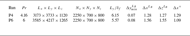


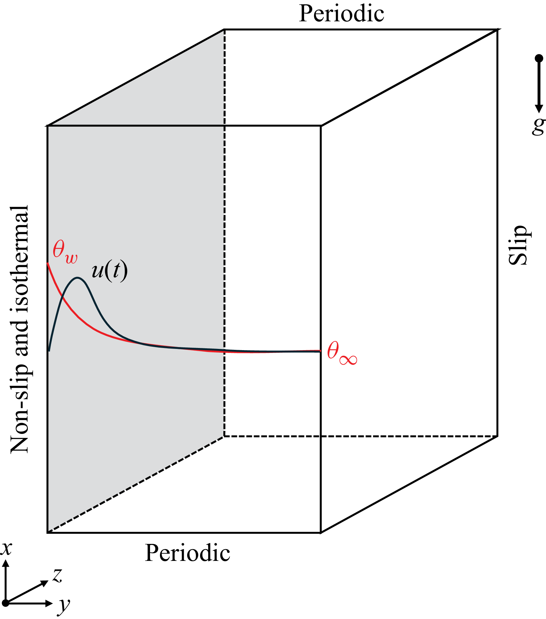

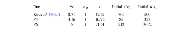


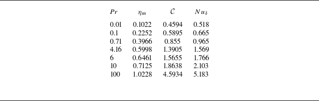


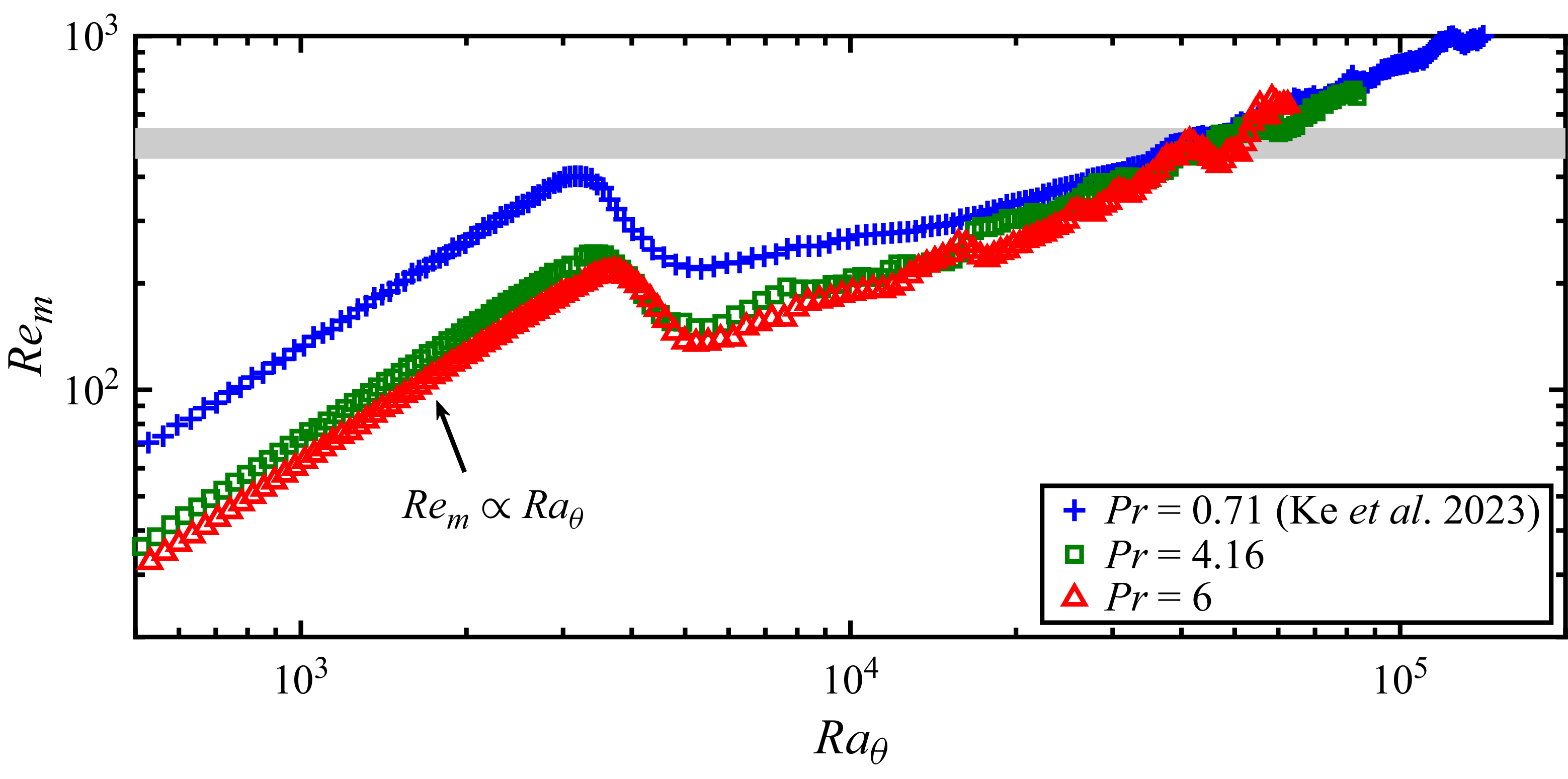


 Open access