2.1 Side-by-side rotor system

Two counter-rotating rotors, separated by one rotor diameter from rotor tip to rotor tip, were installed with their axes perpendicular to a ground plane. Both rotors were two-bladed and comprised a radius $R = 76.2$ mm, with $4''$ pitch and a parabolic tip. These are commercially available under model numbers APC 6X4E and APC 6X4EP (identical but mirrored, for the counter-rotating configuration). The ratio between the ground plane area and rotor disk area was approximately 35. Each rotor was driven by a geared in-runner brushless motor (Hacker, B20 26 L kv2020 + 4:1), at a shaft rotational speed of 167 Hz. Nominally, the blade passing frequency (BPF) was 333 Hz. No phase control between the rotors was present but this was monitored, together with the rotational speed, by using high-speed camera footage. From this followed a constant relative difference in rotational speed of less than 0.25 Hz over the acquisition duration of the measurement. The chord-based Reynolds number is $Re_c = 42\,000$ (with the chord taken at the 0.75$R$ location) and the tip Mach number is $M_t = 0.22$. The rotors were operated with a thrust coefficient of $C_t = 0.117$ and provided $T = 2.14$ N of thrust, in the out-of-ground effect condition. Two different ground stand-off heights were considered during the experiment: $H/R = 2$ and $H/R = 4$. A summary of the operating conditions is presented in table 1.

Table 1.

Side-by-side rotor operating conditions.

2.2 Planar particle image velocimetry (PIV) measurements

Planar PIV measurements were acquired in the domain illustrated in figure 2. The experiment was conducted inside an enclosure of $2 \times 2 \times 3$ m$^3$ that confines the helium-filled soap bubbles (HFSB) used as flow tracers (Reference Faleiros, Tuinstra, Sciacchitano and ScaranoFaleiros, Tuinstra, Sciacchitano, & Scarano, 2019). Any effects of re-circulation in the enclosure are observed at frequencies comparable to the BPF (Reference Weitsman, Stephenson and ZawodnyWeitsman, Stephenson, & Zawodny, 2020) and therefore do not affect the relatively large time scales of interest. Five HFSB generators delivered roughly 150 000 bubbles per second, which were nearly neutrally buoyant and had a mean diameter of 0.4 mm. The enclosure was seeded for two minutes prior to performing the measurement, and resulted in a density of roughly 0.01 particles per pixel corresponding to a spatial concentration of 12 particles cm$^{-2}$. Laser illumination was provided by a Nd:YAG Continuum Mesa PIV 532-120-M laser. The laser beam was expanded by a cylindrical lens allowing a light sheet thickness of 2 cm. Its effective thickness was estimated using three-dimensional (3-D) flow data as 8 mm. The centre of the laser sheet was positioned with an offset of 1.5 cm from the rotor axes (in positive $x$ direction) to avoid shadows from the rotor mounting. Illumination was given with a pulse width of $\delta t = 150$ ns and a rate of 4.0 kHz.

Figure 2.

A 3-D schematic of the experimental apparatus, coordinate system and measurement plane.

A high-speed CMOS camera (Photron Fastcam SA.5, $1024 \times 1024$ px$^2$) was used for imaging and placed outside the closed environment at a distance of 1 m from the measurement region. A lens with focal length $f = 50$ mm and a numerical aperture set to $f_{\#} = 8$ captured a field of view of $38.5 \times 38.5$ cm$^2$ ($5R \times 5R$) at a magnification of $M = 0.053$. Synchronization between the camera and the laser was obtained with a LaVision programmable timing unit (PTU X). Each experimental run captured 2.7 s of data (approximately 11 000 recordings) and was repeated six times, thus providing a total of roughly 16 s ($\approx$2750 rotor revolutions) of discontinuous measurements for each of the two configurations. Measurement parameters are summarized in table 2.

Table 2.

Illumination and imaging conditions.

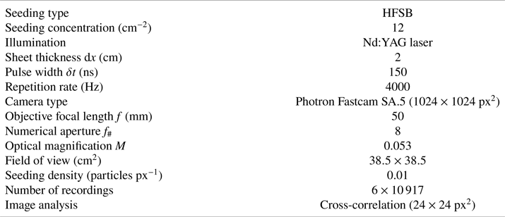
Two pre-processing steps were applied to the raw camera footage before computing PIV-based velocities. First, a minimum time filter was used to eliminate any stationary reflections from the ground plane and support struts of the rotors. Second, a sliding minimum filter with a length scale of 3 pixels was applied to reduce any unsteady rotor-blade reflections. Planar velocity components were inferred by cross-correlation between subsequent images, with a window size of $24 \times 24$ px$^2$ and an overlap of 75 %. This resulted in a vector resolution of 8 mm and a vector spacing of 2 mm. The velocity field was then cropped to a physical domain of $31 \times 27$ cm$^2$. As a final post-processing step, time super-sampling with a factor of 5 was applied to improve the quality of the velocity spectra.

The measurement uncertainty $\epsilon _w$ for the instantaneous velocity field was computed using the method of correlation statistics as described by Reference WienekeWieneke (2015). Values of $\epsilon _w$ were compared to the induced velocity of a single rotor without a ground plane ($w_{ind} = 14.25$ m s$^{-1}$). From this follows an average instantaneous uncertainty of approximately 4 % of the rotor-induced velocity. Conclusions drawn from these data on the large-scale flow dynamics are not affected by this relatively small uncertainty.

2.3 The 3-D dataset

Supplementary to the described experiments, the current work also makes use of a previously performed experiment, where the flow field was measured in a 3-D domain (see Reference Dekker, Ragni, Baars, Scarano and TuinstraDekker et al., 2022). Such data, although encompassing a shorter observation time (1 s in total), bring additional information on the instantaneous flow organization. A short summary of the Reference Dekker, Ragni, Baars, Scarano and TuinstraDekker et al. (2022) dataset is provided here. The HFSB were illuminated by a LaVision LED-Flashlight 300 device in a volume spanning $20 \times 31 \times 33$ cm$^3$. A tomographic imaging set-up comprised three high-speed CMOS cameras (Photron Fastcam SA1.1). Each measurement included 2000 image recordings at a rate of 2.0 kHz. The 3-D particle motion analysis was performed with the ‘shake-the-box’ method (Reference Schanz, Gesemann and SchröderSchanz, Gesemann, & Schröder, 2016). This delivered approximately 10 000 particle tracks for each time step with a maximum particle displacement of 20 pixels (a physical displacement of 6.4 mm). The instantaneous velocity field was reconstructed using the vortex-in-cell technique (VIC+) as described by Reference Schneiders and ScaranoSchneiders and Scarano (2016) for 3-D scattered particle data; calculations were done in DaVis, with the modified algorithm VIC# (Reference Jeon, Müller, Michaelis and WienekeJeon, Müller, Michaelis, & Wieneke, 2018). The instantaneous velocity field was reconstructed on a grid with $h = 3.8$ mm spacing between neighbouring vectors.

3.1 Three-dimensional flow topology

Observations of the unsteady flow behaviour of the multi-rotor system in ground proximity, based on the instantaneous and mean flow fields, are described in this section. An illustration of the fountain phenomenon is shown in figure 3(a), for a ground stand-off distance of four radii. Shown are the instantaneous velocity magnitude (blue) and positive axial velocity iso-surfaces (red); the velocity has been normalized by $w_{ind}$ and is adopted for all results displaying normalized velocity.

Figure 3.

Iso-surfaces of normalized velocity magnitude $V/w_{ind} = 0.5$ (blue) and $w/w_{ind} = 0.25$ (red) for (a) $H/R = 4$ and (b) $H/R = 2$. Iso-surfaces of $\lambda _2 = -60\,000\ {\rm s}^2$ (blue) and $\lambda _2 = -90\,000\ {\rm s}^2$ (red) for (c) $H/R = 4$ and (d) $H/R = 2$. The measurement volume is illustrated by the green box in (a).

In figure 3(a), the rotor slipstreams develop two wall jets that stagnate near the ground plane. The collision of these jets along the stagnation line between the rotors results in the fountain flow, highlighted by the red iso-surfaces, and reaches up to three rotor radii in height. When the ground stand-off distance is reduced to two rotor radii, the fountain remains similar in height (figure 3b) by the balance between the increase of stagnation pressure with reduced height (for constant thrust) and the reduced inflow to the rotor by the presence of the ground. In this case, the fountain reaches above the rotor disk and is inclined towards the left-sided rotor 1. Furthermore, the toroidal separation region in the centre of the wake has increased, as is particularly visible in the wake of rotor 2 not being affected by a re-ingestion. The rotor wake involves tip/root vortices of the blades, as well as the blade section wakes. Due to the relatively high loading in the hover scenario, the tip vortices are the dominant flow features carried to the fountain where they are ejected from the ground. This is confirmed by computing the $\lambda _2$-criterion, which is visualized for both ground stand-off distances in figures 3(c) and 3(d). In figure 3(c), the path of the blade tip vortices is clearly visible close to the blade. They are visible for wake ages up to three to four rotor revolutions before breakdown occurs. Even though the helical structure of the wake is lost after this, coherent structures are still present close to the ground and even within the upward fountain flow. A different phenomenon is present in figure 3(d) for $H/R = 2$, where the wake expands before the vortices break down. Consequently, the vorticity is increased by vortex stretching, similar to what is found for a single rotor in ground proximity (Reference Lee, Leishman and RamasamyLee, Leishman, & Ramasamy, 2010). This is likely to be the reason why larger vortex structures are present in the fountain for the lower ground stand-off distance. Furthermore, since the fountain reached above the rotor disk, coherent structures get re-ingested into rotor 1 (at the time instant of the instantaneous field in figure 3d). Note that the direction of re-ingestion was observed changing back and forth from rotor 1 to rotor 2. This re-ingestion switching occurred at a relatively large time scale, in comparison to 1 s acquisition period of the 3-D data. In order to further focus on the plane of the fountain switching, we proceed with the two-dimensional (2-D) dataset for a more detailed analysis of the velocity distribution. The choice to switch to planar velocimetry data is justified by the limited out-of-plane motions in the fountain plume. On a final note, the two different flow topologies presented in this section were found for constant thrust coefficient $C_t$. Since the height of the fountain is proportional to the induced velocity of the rotors and therefore to the thrust coefficient, it is expected that the minimal ground stand-off height $H/R$ for re-ingestion to occur decreases with increasing thrust.

3.2 Velocity field statistics

In the previous section, an asymmetric re-ingestion was noted on the basis of an instantaneous velocity field. This asymmetry is also noticeable in the time-averaged results of the 2-D velocity measurements, as evidenced by the axial velocity contours and velocity streamlines in figure 4.

Figure 4.

Time-averaged axial velocity contours and 2-D streamlines computed over one acquisition (2.7 s) for (a) $H/R = 4$ and (b) $H/R = 2$. Annotations $n_1$, $n_2$ and $n_3$ denote nodal points in the domain.

For a rotor height of four rotor radii in figure 4(a), the upward fountain flow is inclined towards the slipstream of rotor 1. Effects of the fountain flow inclination are visible throughout the domain: a missing toroidal separation region for the wake where the fountain is inclined towards (compare points A and B), and furthermore, a nodal point, $n_1$, appears near the fountain and highlights the entrainment of air to the fountain (Reference Cabrita, Saddington and KnowlesCabrita et al., 2005). When the rotor ground stand-off distance is reduced to two rotor radii (figure 4b), the fountain flow reaches above the rotor disk, after which it is re-ingested. In figure 4(b), two nodal points $n_2$ and $n_3$ are found with a slight offset in height, and the fountain is inclined towards the side with the lower nodal point. Ultimately, this affects the wake distribution, where rotor 1 has more momentum in the centre of the wake. As for figure 4(a), the toroidal separation regions are also affected in an asymmetric manner (points C and D).

The root mean square of the axial and lateral velocity fluctuations are presented in figure 5 for both ground stand-off distances. In the axial direction, the most intense fluctuations are found in the separation regions below each rotor (see figures 5a and 5b). The fluctuations are also intense along the boundaries of the slipstream, caused by the tip vortices (see points A and B in these figures). Moreover, the fluctuations are stronger in the slipstream of the rotor that re-ingests the fountain flow, which is expected due to the turbulence ingestion. The strongest fluctuations in the lateral direction are found in the stagnation points near the ground (figures 5c and 5d). For the lower rotor ground stand-off distance, the fluctuations comprise a larger magnitude and exhibit a larger extent into the fountain flow.

Figure 5.

Root mean square of velocity fluctuation in axial direction for (a) $H/R = 2$ and (b) $H/R = 4$, and in lateral direction for (c) $H/R = 2$ and (d) $H/R = 4$. Green rectangles denote the regions where the vectors are extracted for generating figure 6.

3.3 Fountain flow dynamics

In order to examine the relation between the fountain flow unsteadiness and the BPF, the pre-multiplied spectrum of the lateral velocity fluctuations is computed, at different heights within the fountain. For the calculation of the spectra, roughly 330 000 samples are collected. These are divided into ensembles of $2^{13}$ samples and processed using the Welch method (50 % overlap) and a Hanning window to reduce any spectral leakage. This results in a frequency resolution of 2.44 Hz (0.015 BPF). The pre-multiplied spectra are presented in figure 6 for three heights and both ground stand-off distances. All energy spectra are dominated with a broadband hump at lower frequencies compared to the BPF. Particularly, in figure 6(a), which is extracted close to the stagnation point near the ground, the fluctuations are energetic at frequencies one to two orders of magnitude lower than the BPF. Higher up within the fountain, towards $z/R = 1.0$ and $z/R = 2.2$ (figures 6b and 6c, respectively), the energy distribution shifts towards slightly higher frequencies by the increase in turbulent fluctuations after the collision of the two opposing wall jets. As discussed in § 3.2, the intensity of the velocity fluctuations increases when re-ingestion takes place (indicated by the arrows in figure 6).

Figure 6.

Pre-multiplied energy spectra of the lateral velocity fluctuations in the centre of the fountain flow, for $H/R = 2$ and $H/R = 4$, and at heights of (a) $z/R = 0.2$, (b) $z/R = 1.0$ and (c) $z/R = 2.2$.

Furthermore, the spectra corresponding to $H/R = 4$ are relatively smooth in comparison with the spectra from the case of $H/R = 2$. The latter comprises distinct peaks at multiples of approximately 7 Hz in figure 6(b), thus indicating that the flow unsteadiness for the $H/R = 2$ case is distinctly different. The occurrence of these spectral peaks is later shown to be related to the re-ingestion switching of the fountain flow.

3.4 Re-ingestion switching cycle and time scale

After having shown the occurrence of a low-frequency unsteadiness in the fountain flow structure, the time-resolved flow field will aid in identifying the spatial–temporal dynamics of this unsteadiness. For the case of $H/R = 2$, re-ingestion occurs at certain time instances (recall figure 3 and its discussion), while other time instances are characterized by the absence of re-ingestion. During these latter instances, the fountain can occasionally reach locations significantly higher than the rotor height. Two sequences in figures 7(a–d) and 7(e–h) show these two different scenarios using sliding averaged results. The length of each sequence is 113 ms, corresponding to an approximate frequency of 8.8 Hz, comparable with the frequency at which the dominant flow fluctuations were identified in § 3.3.

Figure 7.

Normalized velocity magnitude contours $V/w_{ind}$ and 2-D velocity vectors of two time sequences of sliding averages (ensembles of 100 samples/0.25 s), with a temporal increment of ${\rm d}t = 0.0375$ s. The series (a–d) is statistically independent from the series (e–h), with $t_2 = t_1+1.7$ s.

The sequence in figure 7(a–d) starting at $t_1$ captures a relatively stable fountain flow reaching above the rotor disks. Hence, the phenomenon of fountain flow re-ingestion, by one of the two rotors, is minimal. Contrary to this is the statistically independent time sequence starting at $t_2$, shown in figure 7(e–h). In the first frame, the fountain leans towards the right rotor, where re-ingestion takes place at point A. At $t_2+38$ ms, this results in an increase in momentum at point B and the fountain directs towards the left rotor (see point C). In the subsequent frame $t_2+75$ ms, re-ingestion takes place in point D and more momentum towards the centre of the wake is found in point E. Finally, the fountain re-orientates back towards the right rotor, visible in point F. Within a full measurement acquisition period, several similarly looking switching cycles were observed.

The occurrence of the two different flow states described above (fountain flow eruption above the rotor disk and re-ingestion switching) closely resembles a ‘bimodal’ behaviour of a fountain flow associated with impinging, twin jets (Reference Saddington, Cabrita and KnowlesSaddington et al., 2005; Reference Stahl, Prasad and GaitondeStahl et al., 2021) and is suggested to be caused by the orientation of vortical structures in the turbulent wall jet (Reference Stahl, Prasad and GaitondeStahl et al., 2021). On that note, the re-ingestion switching cycle as illustrated in figure 7(e–h) is not present for each sequence investigated along the measurement. Although not shown here for brevity, intermittent intervals of stable re-ingestion to either rotor are also present. On average, this happens more often for rotor 1 compared with rotor 2, which causes the slight inclination of the fountain to rotor 1 when computing the time-averaged results of figure 4. Given the unstable nature of the fountain and the low-Reynolds-number regime in which the rotor blades are operated, the bias is expected to be caused by minor discrepancies in the geometrical/performance parameters between the two rotors. Nonetheless, re-ingestion is still seen to switch along the loop presented in figure 7(e–h) during the majority of the acquisition period. To quantify the re-ingestion switching, a time scale can be assigned for the case of $H/R$ = 2. By following a particle trajectory during re-ingestion, the reciprocal of its velocity is integrated along a path $s$ to compute the convective flow-around time. Note that the velocity $V(s)$ and trajectory length $s$ depend on the system parameters of ground stand-off distance $H$ and rotor thrust $T$. The resultant flow-around time is approximately $T_{conv} \approx 0.1$ s and corresponds to a frequency of $f_{conv}$ = 1/$T_{conv}$ $\approx$ 10 Hz. This value is of the same order as the energy content at 7 Hz (and multiples of that) within the spectra of the lateral velocity fluctuations (figure 6). Furthermore, the flow-around time is representative of the fountain switching to the other rotor and back (see figure 7). Note that the velocity $V(s)$ and trajectory length $s$ depend on the system parameters of ground stand-off distance $H$ and rotor thrust $T$. Hence, for a given ground stand-off distance, and therefore constant trajectory length $s$, the convective frequency $f_{conv}$ is expected to increase with an enhancement of the thrust.

Next, the cycle of re-ingestion switching is explored in further detail in §§ 4 and 5, with a modal analysis to identify its underlying spatial–temporal flow structures.

4.1 Application of classical POD

A POD decomposition is performed using data corresponding to all six acquisition periods for the condition of $H/R = 2$. Thus, the total space–time data consist of $m \approx 65\,000$ temporal snapshots, corresponding to roughly 16 s of data. Spatially, the data of the full field of view are employed. For the POD, the formulation of Reference LumleyLumley (1967) is adopted, known as the classical POD (reviewed by Reference Berkooz, Holmes and LumleyBerkooz, Holmes, & Lumley, 1993). Considering that the amount of snapshots $m$ exceeds the spatial rank of the data ($n \approx 40\,000$), the classical approach is favoured so that ensemble averaging in time can be performed (e.g. Reference GeorgeGeorge, 1988; Reference Tinney, Shipman and PanickarTinney, Shipman, & Panickar, 2020). The decomposition deals with the velocity fluctuations only, computed as

(4.1)\begin{equation} \boldsymbol{u}'(\boldsymbol{x},t) = \boldsymbol{u}(\boldsymbol{x},t)- \bar{\boldsymbol{u}}(\boldsymbol{x}), \quad t = t_1, t_2,\ldots, t_m.\end{equation}

The velocity fluctuations are decomposed in a set of temporal coefficients, $a_i(t)$, and spatial modes, $\boldsymbol {\phi }_{i}(\boldsymbol {x})$, where $i$ is the mode number. A full reconstruction of a single instantaneous field, using all $n$ POD modes, is then generated through

(4.2)\begin{align} \boldsymbol{u}'(\boldsymbol{x},t) = \sum_{i = 1}^n a_{i}(t) \boldsymbol{\phi}_{i}(\boldsymbol{x}). \end{align}

In order to solve for the POD modes and temporal coefficients, an eigenvalue problem is constructed with the spatial modes $\boldsymbol {\phi }_{i}(\boldsymbol {x})$ defined as the eigenvectors of the covariance matrix, or two-point correlation tensor, $\boldsymbol {R}$, following

(4.3)\begin{equation} \boldsymbol{R}\boldsymbol{\phi}_i = \lambda_i\boldsymbol{\phi}_i, \quad \lambda_1\geq \cdots\geq \lambda_n. \end{equation}

The covariance matrix $\boldsymbol {R}$ is generated using ensemble-averaging in time, following

(4.4)\begin{equation} \boldsymbol{R} = \langle \boldsymbol{u}'(\boldsymbol{x},t)\boldsymbol{u}' (\boldsymbol{x}'',t)\rangle, \end{equation}

where the double prime is used to denote separations in space. In (4.3), $\lambda _i$ denotes an ordered sequence of eigenvalues. By indicating the total resolved kinetic energy with $E$, equal to the sum of the eigenvalues, the relative energy fraction of each spatial mode $\boldsymbol {\phi }_i$ is equal to

(4.5)\begin{equation} \tilde{\lambda}_i = \frac{\lambda_i}{\displaystyle \sum_{k = 1}^n \lambda_k} = \frac{\lambda_i}{E}. \end{equation}

Finally, the temporal coefficients $a_i(t)$ can be computed by projecting the original data on the spatial modes, according to

(4.6)\begin{equation} a_i(t) = \int \boldsymbol{u}'(\boldsymbol{x},t) \boldsymbol{\phi}_i(\boldsymbol{x}) \,{\rm d}\boldsymbol{x}. \end{equation}

4.2 Energy distribution and spatial POD mode shapes

Data reduction using the spatial POD ranks the modes according to their relative energy contribution to the total resolved energy in the flow domain. Figure 8 presents the relative energy fraction and cumulative energy for each mode. The system is relatively low-dimensional, given that 70 % of the total resolved energy is captured in less than 100 modes. The energy fractions of the first five modes are 7.0 %, 4.8 %, 4.3 %, 3.9 % and 3.3 %, respectively.

Figure 8.

Energy fraction and cumulative energy as a function of POD mode number $n$.

Figure 9 presents the first five POD mode shapes, split by their lateral and axial velocities. A sketch is included in figure 9(c) to show the contribution of each mode to the time-averaged flow field by highlighting the primary flow features. We now proceed with a brief discussion of each mode.

Figure 9.

The POD mode shapes: (a) $v$ and (b) $w$ component. (c) The contribution of the mode to the flow field when the time coefficient decays from positive unity (black streamlines) to negative unity (blue streamlines).

In the discussion of figure 7(a–d), an intermittent appearance of the fountain rising above the rotor disk was identified. Since no re-ingestion takes place in that case, the flow field is relatively symmetric with a large vertical velocity magnitude between/above the rotors. Mode 1 in figure 9 is representative of this flow state. A sideways inclination of the fountain is captured by mode 2 and predominantly shows activity below the rotor disk. When the associated temporal coefficient would decrease from a positive value to a negative one, the fountain will change inclination from the left rotor to the right. There is also an activity in the axial direction near the wall, showing a relation with the two toroidal separation regions. These two regions simultaneously grow/shrink in size. Similar to mode 1, mode 3 comprises an asymmetric mode shape. Here, most of the energy is contained at the inflow and toroidal separation region of rotor 1. Again, as for mode 2, we see an increase of the separation regions below rotor 1 when re-ingestion goes to the other rotor. Mode 4 contains most of the activity in the axial motions within the separation regions. These motions have opposite sign for the regions associated with rotors 1 and 2, e.g. one separation region grows while the other one shrinks, and vice versa. Finally, mode 5 represents a lateral drifting of the entire fountain column, where a positive time coefficient is associated with the fountain being closer to the left rotor. When time is retained in the analysis, the zero-mean temporal coefficient of each POD mode signifies the degree of activity of the mode, during the measurement time. Temporal coefficients are analysed next to show the dynamic behaviour and mode coupling.

4.3 Temporal POD coefficients

The temporal coefficients are inferred from projecting the raw data back on the POD modes. Recall that six different acquisition periods were used to compute the POD modes. Hence, the corresponding time coefficient of each mode consist of six independent segments, which are presented in figures 10(a) and 10(b) for modes 1 and 2, respectively.

Figure 10.

Temporal POD coefficient of (a) mode 1, $a_1$, and (b) mode 2, $a_2$. Pre-multiplied energy spectra of the temporal coefficients of (c) modes 1 and 3 and (d) modes 2, 4 and 5. The frequency has been normalized by the convective frequency, i.e. $f^*=f/f_{conv}$.

A simple visual inspection of the $a_1$ and $a_2$ time series in figures 10(a) and 10(b) already reveals that mode 1 resides at a lower frequency in comparison with mode 2. This is further explored by computing the energy spectra of the temporal mode coefficients. Pre-multiplied energy spectra, normalized with the resolved energy per mode, are shown in figure 10(c) for both modes 1 and 3 and in figure 10(d) for modes 2, 4 and 5. All spectra were computed with ensemble averaging each of the six segments of data, of which each segment itself was first split into bins of $2^{11}$ samples long (yielding a spectral resolution of ${\rm d}f \approx 2$ Hz). Note that the abscissa has been normalized with the convective frequency: $f^* = f/f_{conv}$ (see § 3.4).

Overall, the energy content resides at low frequencies compared with the BPF, as was already noted in the spectra of the raw, lateral velocity fluctuations presented in figure 6. Most interestingly, modes 2, 4 and 5 comprise a similar spectral distribution, concentrated around the convective frequency. This indicates that these modes are linked to the flow recirculation cycle. The coupling between these three modes is investigated in § 5 through a more detailed analysis of the temporal coefficients.

5.1 Modal coupling

The temporal coupling between modes 2, 4 and 5 is first confirmed by plotting a magnitude of the linear coherence for every combination of two temporal mode coefficients in the range $n = 1$ to 6. First, the linear coherence was computed between temporal coefficients $a_i$ and $a_j$, following

(5.1)\begin{equation} \gamma^2(f) = \frac{\vert G_{a_ia_j}(f) \vert^2}{G_{a_ia_i}(f)G_{a_ja_j}(f)}. \end{equation}

Here $G_{a_ia_i}(f)$ is the energy spectrum of temporal coefficient $a_i(t)$ and $G_{a_ia_j}(f)$ is the cross-spectrum of mode coefficients $a_i(t)$ and $a_j(t)$. The spectral coherence is calculated using windows of $2^{11}$ samples, similar to how the energy spectra of figure 10 were generated. The coherence indicates the fraction of energy corresponding to the coherent fluctuations in $a_i(t)$ and $a_j(t)$; note that $\gamma ^2$ is a normalized quantity, thus $0 \leq \gamma ^2 \leq 1$. When averaging $\gamma ^2$ over a frequency domain of interest, that is, the rate of the re-ingestion switching loop (0.75$f_{conv}\leq f \leq$ 1.25$f_{conv}$), the resultant magnitude $\overline {\gamma ^2}$ is obtained and its amplitude is plotted in figure 11. Here, coherence values between 0.3 and 0.5 are found across the convective frequency domain for the coupling between modes 2, 4 and 5. The coherence magnitudes between the other mode combinations remain below 0.25.

Figure 11.

Coherence magnitude $\overline {\gamma ^2}$ for combinations of temporal mode coefficients, taken as the average coherence value over $0.75 f_{conv}\leq f \leq 1.25 f_{conv}$.

The relation between modes 2, 4 and 5 is further examined in the time domain by computing the cross-correlation between each of the temporal coefficients of these modes. The results in figure 12(a) show a correlation and anti-correlation peak in the proximity of a lag of $\tau$ = 0 s. The zoomed-in plot of figure 12(b) reveals a similar shape of the cross-correlation signal for each of the three mode combinations. First of all, this is characterized by a correlation value of approximately 0.3 at a positive lag, indicated by $\tau _i$. Second, by the orthogonality definition in the modal decomposition, a zero correlation value for $\tau = 0$ s is found. Finally, a weaker but present anti-correlation value is visible at a negative lag, i.e. $\tau < 0$.

Figure 12.

(a) Overview and (b) zoomed-in plot of the temporal cross-correlation coefficient, and corresponding lags for modes 2, 4 and 5. (c) Same as (a,b) but subtraction of lags in (b) and normalization of lag $\tau$ by $T_{conv}$.

The sum of the lags $\tau _i$, effectively creating a loop from mode 2 back to 2 while passing modes 4 and 5, closely resembles the flow-around time introduced in § 3.4, i.e. $\sum \tau _i = 94\ {\rm ms} \approx T_{conv}$. Hence, these modes represent successive, energetic events that occur along the re-ingestion cycle. This apparent cyclic behaviour is also confirmed by translation of the cross-correlation signals. By subtracting the lag $\tau _i$ from figure 12(b) and normalizing $\tau$ by the flow-around time $T_{conv}$ (resulting in figure 12(c). The anti-correlation of each of the mode combinations is now shifted towards a value of 0.5. Moreover, a second positive correlation peak also becomes apparent for a lag value of $-1$, indicating similar behaviour between the modes which is a complete cycle ahead of the dominant correlation peak. The physical interpretation of the combination of modes 2, 4 and 5 and the meaning of their relative lag $\tau _i$ will become clear from a low-order reconstruction presented next.

5.2 Low-order reconstruction

The reduced-order flow with its energetic features will allow for a description of dynamic flow features that are a part of establishing the cycle of re-ingestion switching. The coupling between these modes is reconstructed using a pseudo time coefficient $b_i$, based on a harmonic wave of frequency $f_{conv}$, over a time interval of $0\leq t \leq 1.75 T_{conv}$, following

(5.2)\begin{equation} b_i = \sin(2\pi f_{conv}t + \psi_i) , \quad 0 \leq t \leq 1.75 T_{conv}. \end{equation}

Here the relative phase offset $\psi _i$ between the time coefficients $b_i$ is based on the sum of the cross-correlation lag $\tau _i$ between the modes:

(5.3)\begin{equation} \psi_i = 2\pi f_{conv} \sum_i\tau_i, \quad i \in\{2, 4, 5\}. \end{equation}

Figure 13 presents the adapted time coefficients $b_i$ computed from (5.2). The original temporal coefficients $a_i$, derived directly from the time-resolved velocity field, have a different shape from what is presented in figure 13. However, the purpose of using the pseudo time coefficients $b_i$ is to show how the modes statistically combine during the flow re-ingestion cycle.

Figure 13.

Pseudo time coefficients $b_i$ used for the low-order reconstruction. Intervals I, II and III indicate the time domains for velocity field reconstructions in figures 14(a), 14(b) and 14(c), respectively.

Sticking to the temporal simplification of harmonic waves, the velocity field can be reconstructed by the sum of the spatial modes 2, 4 and 5, multiplied by their corresponding time coefficient $b_i$, so that

(5.4)\begin{align} \hat{\boldsymbol{u}}(\boldsymbol{x},t) = \bar{\boldsymbol{u}}(\boldsymbol{x}) + \sum_{i}b_i(t)\phi_i(\boldsymbol{x}), \quad i\in\{2, 4, 5\}. \end{align}

By examining the reconstructed velocity field $\hat {\boldsymbol {u}}$, three successive events can be identified within the trajectory of re-ingestion. These events are investigated independently by the definition of spatial and temporal subdomains in the reconstructed velocity field $\hat {\boldsymbol {u}}$, denoted by I, II and III. These time interval are highlighted by the grey zones in figure 13. The spatial subdomains of I, II and III are based on a trajectory of re-ingestion to rotor 1, which is split into three parts. These spatial subdomains, alongside the corresponding time series of the reconstructed velocity field $\hat {\boldsymbol {u}}$, are presented in figure 14.

Figure 14.

Normalized velocity magnitude contours $V/w_{ind}$ of the reconstructed velocity field $\hat {u}$, visualized along the trajectory of re-ingestion to highlight successive critical events. (a) Convection of ejected structures to the inflow of rotor 1, (b) dynamic pressure increase in the wake and (c) lateral drifting of the saddle point. The left-hand plots in (a–c) illustrate the spatial domain, based on the trajectory of re-ingestion (blue arrow), corresponding to the time intervals of figure 13.

The three sequential events of figure 14(a–c) present the core mechanism of the flapping of the fountain and the re-ingestion switching. Subdomain I, illustrated in figure 14(a), shows three successive snapshots. The first of which, at $t/T_{conv} = 0.11$, presents the emerging fountain from the ground with an inclination towards the left. The fountain is then convected upwards and re-ingested into rotor 1 in the final snapshot at $t/T_{conv} = 0.58$. After re-ingestion, the momentum in the slipstream increases, as shown in figure 14(b). Stagnation in the centre of the slipstream, as indicated in the left snapshot, is removed and an attachment of the wake to the ground positions itself laterally below the rotor axis, at $t/T_{conv} = 1.00$. With more lateral momentum in the wall jet, the foot of the fountain drifts towards the right (see figure 14c). After this, ejection from the ground is inclined towards the right rotor, and the cycle is repeated in mirrored orientation. Each of the three events in figure 14 also resembles the results of the time-resolved flow-field analysis in figure 7.

One should note that, by the bias of the time-averaged flow field, the cycle of re-ingestion towards the right rotor is less pronounced. However, the same dynamic features are present. Moreover, as noted in § 3.4, intervals of stable re-ingestion to either rotor are also found, which means that re-ingestion does not switch after every flow-around cycle. During these intervals, the stronger wall jet is not able to push the foot of the fountain far enough towards the other rotor for the switch to occur. For completeness, the re-ingestion switching cycle, along with the corresponding (statistical) delays between the events, are schematically represented in figure 15.

Figure 15.

Schematic representation of events during the re-ingestion of the fountain column.

In the schematic of the re-ingestion loop of figure 15, the first three events show the observations as seen in figures 14(a) and 14(b). In the fourth event of figure 15, the fountain is seen to drift towards the right, as seen by the middle snapshot in figure 14(c). This completes the loop after a time delay of $T_{conv}$ from the first event. After this follow two possibilities: either the cycle is repeated with the same orientation but with a more pronounced inclination of the fountain, or the stagnation point has drifted far enough to the subsequent rotor to allow the re-ingestion to switch, effectively repeating the loop in mirrored orientation.