


1. Introduction
Basaltic fissure eruptions are the most common type of volcanic eruption on Earth (Sigurdsson Reference Sigurdsson, Sigurdsson, Houghton, Rymer, Stix and McNutt2000). Recent examples include the eruption of Kilauea’s Lower East Rift Zone (USA) in 2018 (Neal et al. Reference Neal2019) and the ongoing sequence of eruptions on the Reykjanes Peninsular (Iceland) that began in 2021 (Troll et al. Reference Troll, Deegan, Thordarson, Tryggvason, Krmíček, Moreland, Lund, Bindeman, Höskuldsson and Day2024). A fissure eruption occurs when a dyke – a magma-filled crack – intersects the Earth’s surface, creating an elongated eruptive vent. The eruption typically onsets as a near-continuous curtain of lava fountaining, which localises over hours to days into discrete vents that produce isolated lava fountains and feed lava flows (e.g. Richter et al. Reference Richter, Eaton, Murata, Ault and Krivoy1970; Thorarinsson et al. Reference Thorarinsson, Steinthórsson, Einarsson, Kristmannsdóttir and Oskarsson1973; Delaney & Pollard Reference Delaney and Pollard1982; Eibl et al. Reference Eibl, Bean, Jónsdóttir, Höskuldsson, Thordarson, Coppola, Witt and Walter2017). The hazard posed by a fissure eruption evolves as the fissure localises; in particular, the path taken by fissure-fed lava flows is strongly influenced by the vent location (Rongo et al. Reference Rongo, Lupiano, Spataro, D’ambrosio, Iovine and Crisci2016). Understanding the spatio-temporal evolution of a localising fissure eruption is, therefore, an important practical goal for the management of eruption hazards, as well as a problem of fundamental fluid dynamic interest.
Localisation is thought to arise from a thermoviscous instability, analogous to classical Saffmann–Taylor viscous fingering, by which hot, low-viscosity magma displaces cooled, higher viscosity fluid. The system becomes unstable to the formation of fingers of lower viscosity fluid (Pearson, Shah & Vieira Reference Pearson, Shah and Vieira1973; Whitehead & Helfrich Reference Whitehead and Helfrich1991; Helfrich Reference Helfrich1995; Wylie & Lister Reference Wylie and Lister1995; Morris Reference Morris1996; Wylie et al. Reference Wylie, Helfrich, Dade, Lister and Salzig1999) which become preferred transport pathways that feed localised flow. Bruce & Huppert (Reference Bruce and Huppert1989) suggested that the localisation process could be driven by a feedback between solidification at the walls and the resulting effect on heat advection through the fissure due to the evolving fissure geometry. However, Wylie et al. (Reference Wylie, Helfrich, Dade, Lister and Salzig1999) argued that the localisation that occurs via this feedback evolves on a longer time scale than the localisation caused by thermoviscous fingering, making the latter the dominant effect. Other work has explored the potential role of other processes in localisation, including dynamic wall rock deformation (Ida Reference Ida1992), drain-back of erupted lava (Jones et al. Reference Jones, Llewellin, Houghton, Brown and Vye-Brown2017), formation of plumes of decoupled bubbles of magmatic gas (Pioli et al. Reference Pioli, Azzopardi, Bonadonna, Brunet and Kurokawa2017; Houghton et al. Reference Houghton, Tisdale, Llewellin, Taddeucci, Orr, Walker and Patrick2021) and convective exchange flow within the dyke (Jones & Llewellin Reference Jones and Llewellin2021).
Previous work on thermoviscous localisation has made the simplifying assumption that magmatic dykes have walls that are initially planar and parallel. However, dyke emplacement involves pulsatory, stochastic failure of heterogeneous country rock (Allgood et al. Reference Allgood, Llewellin, Humphreys, Mathias, Brown and Vye-Brown2024), resulting in dykes that vary substantially in thickness along their length (Daniels et al. Reference Daniels, Kavanagh, Menand and Sparks2012; Parcheta et al. Reference Parcheta, Fagents, Swanson, Houghton and Ericksen2015). In this study, we explore the role that the non-planar geometry of dyke walls plays in localisation. We consider the flow of a viscous fluid with temperature-dependent viscosity through a dyke with variations in thickness along its length (i.e. the gap thickness varies perpendicular to the main flow direction; see figure 1). The full equations are reduced, taking advantage of the small aspect ratio of fissure width to length, as well as a number of additional physical assumptions, given in § 2. Furthermore, we employ a heat balance approach, detailed in § 2.1, to account for the temperature and viscosity field when averaging across the fissure width. A similar averaging approach has been used in a number of studies concerning cooling lava flows (Balmforth, Craster & Sassi Reference Balmforth, Craster and Sassi2004; Bernabeu, Saramito & Smutek Reference Bernabeu, Saramito and Smutek2016; Thorey & Michaut Reference Thorey and Michaut2016; Hyman, Dietterich & Patrick Reference Hyman, Dietterich and Patrick2022; Moyers-Gonzalez et al. Reference Moyers-Gonzalez, Hewett, Cusack, Kennedy and Sellier2023), as it maintains the key structure of the across-flow temperature profile in the model, while providing the numerical efficiency of averaging over the thin dimension of the flow. We first quantify behaviour in a dyke with sinusoidally varying width, constraining the role of amplitude and wavelength of the variation, and of the pressure difference driving the flow. We find that, under volcanologically relevant conditions, the thermoviscous fingering instability can be overprinted by the effect of geometry, which focusses hotter, faster flow into the wider portions of the dyke, and cooler, slower flow into the narrower portions. We then demonstrate the importance of this localisation mechanism in a more realistic dyke geometry, consistent with field observations (Parcheta et al. Reference Parcheta, Fagents, Swanson, Houghton and Ericksen2015) and country-rock fracture patterns (Brodsky, Kirkpatrick & Candela Reference Brodsky, Kirkpatrick and Candela2016).
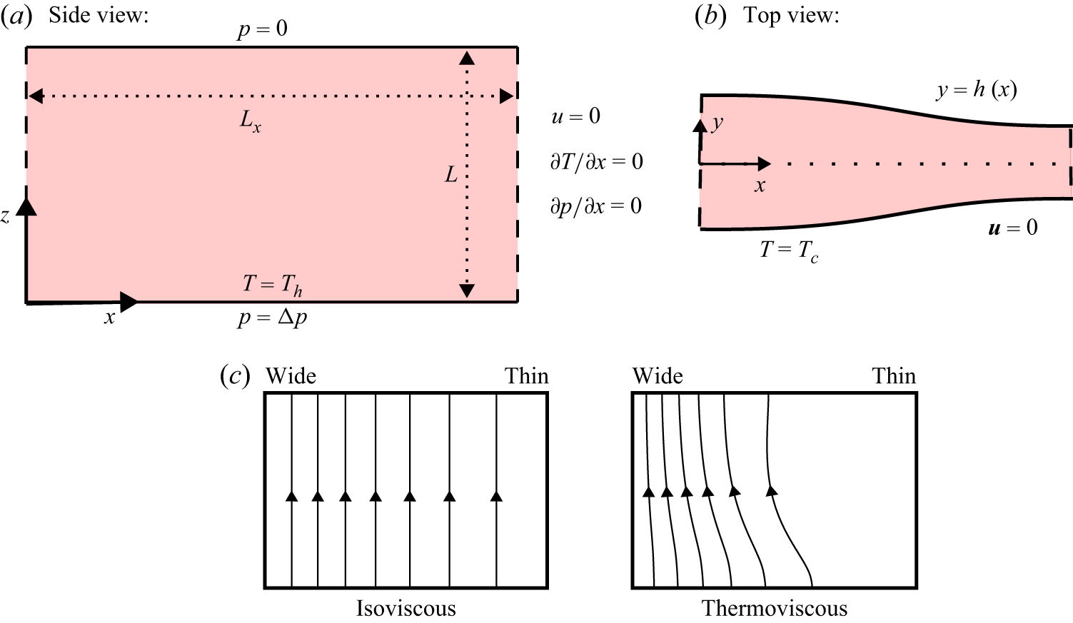
(a,b) Schematic of fissure geometry, coordinate system and boundary conditions. In the side view, panel (a), the bottom and top boundaries are the inflow and outflow, respectively, the dashed lines indicate no flux (symmetry) boundaries, and the double-headed arrows indicate the vertical and along-fissure length scales. In the top view, panel (b), the bottom and top boundaries are the side walls of the fissure, the dashed lines indicate no flux (symmetry) boundaries, and the dotted line indicates the assumed plane of symmetry down the centreline of the fissure. (c) Diagram indicating the effect that thermoviscosity has on the streamlines of volume flux in such a geometry. For an isoviscous fluid and the topography aligned with the flow direction, the streamlines are parallel. When the viscosity depends on temperature, the streamlines are diverted and flux is concentrated more strongly in the wider region of the fissure.
2. Problem definition
We consider a viscous fluid flowing through a narrow fissure. Figure 1(a,b) shows a diagram of the fissure geometry. We define a coordinate system such that
 $z$
measures distance up the fissure in the (vertical) primary flow direction,
$z$
measures distance up the fissure in the (vertical) primary flow direction,
 $y$
measures distance across the narrow dimension of the fissure and
$y$
measures distance across the narrow dimension of the fissure and
 $x$
measures distance along the fissure. The fissure height is
$x$
measures distance along the fissure. The fissure height is
 $L$
and its half-width varies via a prescribed dependence,
$L$
and its half-width varies via a prescribed dependence,
 $h(x,z)$
, with a typical value of
$h(x,z)$
, with a typical value of
 $h_0\ll L$
. We will consider the width to be independent of
$h_0\ll L$
. We will consider the width to be independent of
 $z$
and, in particular, predominantly impose a sinusoidal variation of the half-width,
$z$
and, in particular, predominantly impose a sinusoidal variation of the half-width,
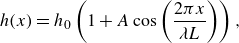 \begin{equation} h(x)=h_0\left (1+A\cos \left (\frac {2\pi x}{\lambda L}\right )\right ), \end{equation}
where
 $\lambda$
is the wavelength of the variation, non-dimensionalised by
$\lambda$
is the wavelength of the variation, non-dimensionalised by
 $L$
. The independence of
$L$
. The independence of
 $h$
on
$h$
on
 $z$
is not a requirement of the model and, in practice, there is likely to be some variation in this direction; however, we anticipate that variations in the
$z$
is not a requirement of the model and, in practice, there is likely to be some variation in this direction; however, we anticipate that variations in the
 $x$
-direction will couple most strongly with the advection of heat and, therefore, be most significant in driving flow localisation. For the sinusoidally varying geometry, the horizontal section considered in the model is of length
$x$
-direction will couple most strongly with the advection of heat and, therefore, be most significant in driving flow localisation. For the sinusoidally varying geometry, the horizontal section considered in the model is of length
 $L_x=\lambda L/2$
, such that a single half-wavelength fits inside the domain. The assumption of symmetry boundary conditions then restricts to symmetrical solutions that are periodic with the same wavelength as the geometry. Figure 1(c) shows the effect of thermoviscosity for the flow through such a geometry, with topography aligned with the (vertical) pressure gradient. For an isoviscous fluid, the streamlines would remain aligned in the vertical direction, with a flux that varies with the cube of the local width, as per Darcy flow. For a temperature-dependent viscosity, however, the viscosity gradients arising from differential cooling drive the streamlines away from the thinner region and towards the wider region of the fissure. This provides the essential mechanism by which localisation is enhanced.
$L_x=\lambda L/2$
, such that a single half-wavelength fits inside the domain. The assumption of symmetry boundary conditions then restricts to symmetrical solutions that are periodic with the same wavelength as the geometry. Figure 1(c) shows the effect of thermoviscosity for the flow through such a geometry, with topography aligned with the (vertical) pressure gradient. For an isoviscous fluid, the streamlines would remain aligned in the vertical direction, with a flux that varies with the cube of the local width, as per Darcy flow. For a temperature-dependent viscosity, however, the viscosity gradients arising from differential cooling drive the streamlines away from the thinner region and towards the wider region of the fissure. This provides the essential mechanism by which localisation is enhanced.
Neglecting viscous heating and thermal expansion, and making the lubrication approximation, the governing equations for the temperature,
 $T$
, pressure (modified to include the hydrostatic contribution),
$T$
, pressure (modified to include the hydrostatic contribution),
 $p$
, and velocity,
$p$
, and velocity,
 $\boldsymbol{u}=(u,v,w)$
, are given to leading order by (cf. Wylie & Lister Reference Wylie and Lister1995)
$\boldsymbol{u}=(u,v,w)$
, are given to leading order by (cf. Wylie & Lister Reference Wylie and Lister1995)
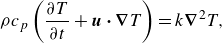 \begin{gather} \rho c_p\left (\frac {\partial T}{\partial t}+\boldsymbol{u\cdot \boldsymbol{\nabla}} T\right ) = k\boldsymbol{\nabla} ^2 T, \end{gather}
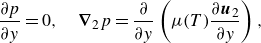 \begin{gather} \frac {\partial p}{\partial y}=0, \quad \boldsymbol{\nabla} _2 p =\frac {\partial }{\partial y}\left (\mu (T)\frac {\partial \boldsymbol{u}_2}{\partial y}\right ), \end{gather}
 \begin{gather} \boldsymbol{\boldsymbol{\nabla} \cdot u}=0, \end{gather}
where
 $\rho$
is the fluid density,
$\rho$
is the fluid density,
 $c_p$
is the specific heat capacity,
$c_p$
is the specific heat capacity,
 $k\equiv \rho c_p\kappa$
is the thermal conductivity,
$k\equiv \rho c_p\kappa$
is the thermal conductivity,
 $\mu (T)$
is the temperature-dependent viscosity, specified later, and
$\mu (T)$
is the temperature-dependent viscosity, specified later, and
 $\boldsymbol{u}_2=(u,0,w)$
and
$\boldsymbol{u}_2=(u,0,w)$
and
 $\boldsymbol{\nabla} _2=(\partial _x, 0,\partial _z)$
are the velocity and gradient in the plane of the fissure. These equations represent conservation of heat, conservation of momentum and incompressibility, respectively.
$\boldsymbol{\nabla} _2=(\partial _x, 0,\partial _z)$
are the velocity and gradient in the plane of the fissure. These equations represent conservation of heat, conservation of momentum and incompressibility, respectively.
Figure 1 shows the prescribed boundary conditions on the temperature,
 $T$
, pressure,
$T$
, pressure,
 $p$
, and velocity,
$p$
, and velocity,
 $\boldsymbol{u}$
. The fluid is assumed to enter at a hot source temperature,
$\boldsymbol{u}$
. The fluid is assumed to enter at a hot source temperature,
 $T_h$
, and with a prescribed pressure,
$T_h$
, and with a prescribed pressure,
 $\Delta p \gt 0$
, at
$\Delta p \gt 0$
, at
 $z=0$
. At
$z=0$
. At
 $x=0$
and
$x=0$
and
 $x=L_x$
, we assume symmetry conditions,
$x=L_x$
, we assume symmetry conditions,
 $u=\partial p/\partial x=\partial T/\partial x=0$
. At the outflow,
$u=\partial p/\partial x=\partial T/\partial x=0$
. At the outflow,
 $z=L$
, the pressure is atmospheric,
$z=L$
, the pressure is atmospheric,
 $p=0$
. We assume no-slip,
$p=0$
. We assume no-slip,
 $\boldsymbol{u}=0$
, and a fixed cold temperature,
$\boldsymbol{u}=0$
, and a fixed cold temperature,
 $T=T_c$
, on the fissure walls,
$T=T_c$
, on the fissure walls,
 $y=\pm h$
. While this fixed temperature boundary condition is a significant simplification of the full thermodynamic conditions at the fissure walls, it is chosen for simplicity and consistency with previous work on the problem (Helfrich Reference Helfrich1995; Wylie & Lister Reference Wylie and Lister1995; Morris Reference Morris1996; Wylie et al. Reference Wylie, Helfrich, Dade, Lister and Salzig1999). Similarly, for comparison to previous work, we assume an exponential dependence of viscosity on temperature
$y=\pm h$
. While this fixed temperature boundary condition is a significant simplification of the full thermodynamic conditions at the fissure walls, it is chosen for simplicity and consistency with previous work on the problem (Helfrich Reference Helfrich1995; Wylie & Lister Reference Wylie and Lister1995; Morris Reference Morris1996; Wylie et al. Reference Wylie, Helfrich, Dade, Lister and Salzig1999). Similarly, for comparison to previous work, we assume an exponential dependence of viscosity on temperature
 \begin{equation} \mu = \mu _0 \exp {\left (-\beta \left (T-T_0\right )\right )}, \end{equation}
where
 $T_0$
and
$T_0$
and
 $\mu _0$
are a reference temperature and viscosity, and
$\mu _0$
are a reference temperature and viscosity, and
 $\beta$
is a parameter that measures the strength of the dependence. This model, which has been used in previous fluid dynamical modelling of thermoviscous localisation, has also been proposed to capture the viscosity of molten basalt as a function of temperature in a number of other studies (Shaw Reference Shaw1969; Spera, Yuen & Kirschvink Reference Spera, Yuen and Kirschvink1982; Dragoni Reference Dragoni1989). More commonly, this dependence is parametrised by an Arrhenius viscosity law (McBirney & Murase Reference McBirney and Murase1984),
$\beta$
is a parameter that measures the strength of the dependence. This model, which has been used in previous fluid dynamical modelling of thermoviscous localisation, has also been proposed to capture the viscosity of molten basalt as a function of temperature in a number of other studies (Shaw Reference Shaw1969; Spera, Yuen & Kirschvink Reference Spera, Yuen and Kirschvink1982; Dragoni Reference Dragoni1989). More commonly, this dependence is parametrised by an Arrhenius viscosity law (McBirney & Murase Reference McBirney and Murase1984),
 $\mu =\mu _\infty \exp (B/T )$
, sufficiently far from the glass transition, or via the Vogel–Fulcher–Tammann (VFT) equation (Giordano, Russell & Dingwell Reference Giordano, Russell and Dingwell2008),
$\mu =\mu _\infty \exp (B/T )$
, sufficiently far from the glass transition, or via the Vogel–Fulcher–Tammann (VFT) equation (Giordano, Russell & Dingwell Reference Giordano, Russell and Dingwell2008),
 $\mu = \mu _\infty \exp (B/(T-T_g) )$
, when nearer the glass transition (at
$\mu = \mu _\infty \exp (B/(T-T_g) )$
, when nearer the glass transition (at
 $T=T_g$
). In any case, the exponential viscosity dependence (2.5) can be viewed as a linearisation of the argument of the exponential in a general dependence of the form
$T=T_g$
). In any case, the exponential viscosity dependence (2.5) can be viewed as a linearisation of the argument of the exponential in a general dependence of the form
 $\mu =\exp (f(T))$
, by writing
$\mu =\exp (f(T))$
, by writing
 $T=T_0+(T-T_0)$
and assuming
$T=T_0+(T-T_0)$
and assuming
 $T-T_0$
small (compared with
$T-T_0$
small (compared with
 $T_0$
in the case of the Arrhenius law or compared with
$T_0$
in the case of the Arrhenius law or compared with
 $T_0-T_g$
in the case of the VFT equation).
$T_0-T_g$
in the case of the VFT equation).
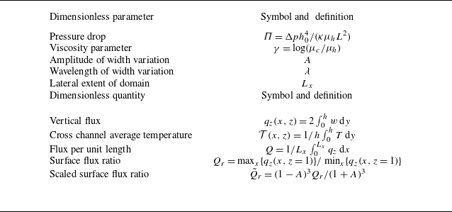
Definition of dimensionless parameters and evaluated quantities.
Following Wylie & Lister (Reference Wylie and Lister1995), we introduce dimensionless variables via
 \begin{gather} \hat {t}\equiv \frac {\kappa }{h_0^2}t, \quad \hat {y}\equiv \frac {y}{h_0}, \quad (\hat {x},\hat {z})\equiv \frac {1}{L}(x,z), \quad (\hat {u},\hat {w})\equiv \frac {h_0^2}{\kappa L}(u,w), \quad \hat {v}\equiv \frac {h_0}{\kappa }v, \quad \hat {p}\equiv \frac {p}{\Delta p}, \end{gather}
 \begin{gather} \hat {T}\equiv \frac {T-T_c}{T_h-T_c},\quad \hat {\mu }(\hat {T})\equiv \frac {\mu (T)}{\mu _h} = \exp (\gamma (1-\hat {T})), \quad \hat {h}\equiv \frac {h}{h_0}, \end{gather}
where
 $\mu _h=\mu (T_h)$
(similarly, we define
$\mu _h=\mu (T_h)$
(similarly, we define
 $\mu _c=\mu (T_c)$
) and
$\mu _c=\mu (T_c)$
) and
 $\gamma =(T_h-T_c)\beta$
. For the sinusoidal geometry, the dimensionless half-width is given by
$\gamma =(T_h-T_c)\beta$
. For the sinusoidal geometry, the dimensionless half-width is given by
 $\hat {h}=1+A\cos (2\pi \hat {x}/\lambda )$
. After non-dimensionalising, the lateral extent of the domain is
$\hat {h}=1+A\cos (2\pi \hat {x}/\lambda )$
. After non-dimensionalising, the lateral extent of the domain is
 $\hat {L}_x=L_x/L$
. The one difference here from the scalings adopted by Wylie & Lister (Reference Wylie and Lister1995) is that we have scaled the pressure by
$\hat {L}_x=L_x/L$
. The one difference here from the scalings adopted by Wylie & Lister (Reference Wylie and Lister1995) is that we have scaled the pressure by
 $\Delta p$
, rather than
$\Delta p$
, rather than
 $ \kappa \mu _h L^2 / h_0^4$
. The result is that a dimensionless pressure drop,
$ \kappa \mu _h L^2 / h_0^4$
. The result is that a dimensionless pressure drop,
 \begin{equation} \Pi = \frac {\Delta p h_0^4}{\kappa \mu _h L^2}, \end{equation}
appears in our governing equations, rather than in the boundary condition for
 $\hat {p}$
. We make the same assumptions of large Péclet number,
$\hat {p}$
. We make the same assumptions of large Péclet number,
 ${Pe}\equiv \Delta p h_0^3/\kappa \mu _h L \gg 1$
, and large Prandtl number,
${Pe}\equiv \Delta p h_0^3/\kappa \mu _h L \gg 1$
, and large Prandtl number,
 ${Pr}\equiv \mu _h/\rho \kappa \gg 1$
. In using the lubrication approximation (2.3), we have assumed a small aspect ratio,
${Pr}\equiv \mu _h/\rho \kappa \gg 1$
. In using the lubrication approximation (2.3), we have assumed a small aspect ratio,
 $\epsilon \equiv h_0/L\ll 1$
, and negligible inertia, which requires that the modified Reynolds number is small,
$\epsilon \equiv h_0/L\ll 1$
, and negligible inertia, which requires that the modified Reynolds number is small,
 ${\epsilon}{Re}\equiv \epsilon \rho \Delta p h_0^3/\mu _h^2 L\ll 1$
. A further assumption required in our non-uniform geometry is that
${\epsilon}{Re}\equiv \epsilon \rho \Delta p h_0^3/\mu _h^2 L\ll 1$
. A further assumption required in our non-uniform geometry is that
 $\lambda \gg \epsilon$
, which ensures the length scale of variations in the
$\lambda \gg \epsilon$
, which ensures the length scale of variations in the
 $x$
-direction remains significantly larger than the cross-channel length scale. At leading order, after dropping hats on all dimensionless variables, the dimensionless governing equations are
$x$
-direction remains significantly larger than the cross-channel length scale. At leading order, after dropping hats on all dimensionless variables, the dimensionless governing equations are
 \begin{align} \frac {\partial T}{\partial t}+\boldsymbol{u}_2\boldsymbol{\cdot}\boldsymbol{\nabla} _2 T + v\frac {\partial T}{\partial y}= \frac {\partial ^2 T}{\partial y^2}, \quad \frac {\partial }{\partial y}\left (\mu (T)\frac {\partial \boldsymbol{u}_2}{\partial y}\right )=\Pi \boldsymbol{\nabla} _2 p, \quad \boldsymbol{\nabla} _2\boldsymbol{\cdot} \boldsymbol{u}_2+\frac {\partial v}{\partial y}=0, \end{align}
where
 $p=p(x,z)$
. Table 1 lists the key dimensionless parameters of the model and the dimensionless quantities we later report for our solutions.
$p=p(x,z)$
. Table 1 lists the key dimensionless parameters of the model and the dimensionless quantities we later report for our solutions.
For parameter values appropriate for a typical Hawaiian fissure eruption, we take: thermal diffusivity
 $\kappa \approx 5\times 10^{-7}$
m
$\kappa \approx 5\times 10^{-7}$
m
 $^{2}$
s–1 (Kilburn Reference Kilburn, Sigurdsson, Houghton, Rymer, Stix and NcNutt2000); cross-channel length scale of
$^{2}$
s–1 (Kilburn Reference Kilburn, Sigurdsson, Houghton, Rymer, Stix and NcNutt2000); cross-channel length scale of
 $h_0\approx 0.25$
m (Walker Reference Walker1986); fissure height of
$h_0\approx 0.25$
m (Walker Reference Walker1986); fissure height of
 $L\approx 1$
km (e.g. Anderson et al. Reference Anderson, Shea, Lynn, Montgomery-Brown, Swanson, Patrick, Shiro and Neal2024); and initial viscosity,
$L\approx 1$
km (e.g. Anderson et al. Reference Anderson, Shea, Lynn, Montgomery-Brown, Swanson, Patrick, Shiro and Neal2024); and initial viscosity,
 $\mu _h\approx 300$
Pa s (Soldati, Houghton & Dingwell Reference Soldati, Houghton and Dingwell2021). The pressure drop,
$\mu _h\approx 300$
Pa s (Soldati, Houghton & Dingwell Reference Soldati, Houghton and Dingwell2021). The pressure drop,
 $\Delta p$
, arises primarily from the difference between the lithostatic pressure of the country rock and the hydrostatic pressure of the magma at the depth of the source. Taking the density of the country rock to be
$\Delta p$
, arises primarily from the difference between the lithostatic pressure of the country rock and the hydrostatic pressure of the magma at the depth of the source. Taking the density of the country rock to be
 $2500$
kg m–
$2500$
kg m–
 $^{3}$
(Moore Reference Moore2001) and the (vesicular) basaltic magma to have a density of
$^{3}$
(Moore Reference Moore2001) and the (vesicular) basaltic magma to have a density of
 $1500$
kg m–
$1500$
kg m–
 $^{3}$
, this gives
$^{3}$
, this gives
 $\Delta p \approx 10^7$
Pa for a source depth of 1 km, which is a feasible depth for the shallow crustal reservoirs that are thought to feed many fissure eruptions (e.g. Anderson et al. Reference Anderson, Shea, Lynn, Montgomery-Brown, Swanson, Patrick, Shiro and Neal2024). At this pressure drop, and the physical quantities assumed previously, we have
$\Delta p \approx 10^7$
Pa for a source depth of 1 km, which is a feasible depth for the shallow crustal reservoirs that are thought to feed many fissure eruptions (e.g. Anderson et al. Reference Anderson, Shea, Lynn, Montgomery-Brown, Swanson, Patrick, Shiro and Neal2024). At this pressure drop, and the physical quantities assumed previously, we have
 $\epsilon =2.5\times 10^{-4}\ll 1$
,
$\epsilon =2.5\times 10^{-4}\ll 1$
,
 $\epsilon {Re}=4\times 10^{-4}\ll 1$
,
$\epsilon {Re}=4\times 10^{-4}\ll 1$
,
 ${Pe}=1\times 10^6\gg 1$
and
${Pe}=1\times 10^6\gg 1$
and
 ${Pr}=6\times 10^5\gg 1$
, all satisfying the assumptions in the reduction of the governing equations. A typical value of the dimensionless pressure drop is around
${Pr}=6\times 10^5\gg 1$
, all satisfying the assumptions in the reduction of the governing equations. A typical value of the dimensionless pressure drop is around
 $\varPi =260$
, though this is likely to vary throughout an eruption, in particular reducing from a large value at the beginning of an eruption to a smaller value as the eruption wanes. An alternative scaling argument instead relies on observations of typical eruptive fluxes and an inference of the corresponding driving pressure drop (e.g. see Delaney & Pollard Reference Delaney and Pollard1982). Tilling et al. (Reference Tilling, Christiansen, Duffield, Endo, Holcomb, Koyanagi, Peterson and Unger1987) report estimates of erupted lava volumes over given time periods during the 1972–1974 Mauna Ulu eruption of Kilauea volcano. These estimates only provide a rough estimate of instantaneous eruptive rates and are likely lower bounds since they are based on lava volume remaining on the surface, excluding material that drained back into the fissures before the eruption ended. Nonetheless, from these figures, we can obtain a typical flux of between 0.001 and 0.05 m
$\varPi =260$
, though this is likely to vary throughout an eruption, in particular reducing from a large value at the beginning of an eruption to a smaller value as the eruption wanes. An alternative scaling argument instead relies on observations of typical eruptive fluxes and an inference of the corresponding driving pressure drop (e.g. see Delaney & Pollard Reference Delaney and Pollard1982). Tilling et al. (Reference Tilling, Christiansen, Duffield, Endo, Holcomb, Koyanagi, Peterson and Unger1987) report estimates of erupted lava volumes over given time periods during the 1972–1974 Mauna Ulu eruption of Kilauea volcano. These estimates only provide a rough estimate of instantaneous eruptive rates and are likely lower bounds since they are based on lava volume remaining on the surface, excluding material that drained back into the fissures before the eruption ended. Nonetheless, from these figures, we can obtain a typical flux of between 0.001 and 0.05 m
 $^{3}$
s–1 per metre length of fissure. This becomes non-dimensionalised by the scale
$^{3}$
s–1 per metre length of fissure. This becomes non-dimensionalised by the scale
 $\kappa L/h_0\approx 0.002$
m
$\kappa L/h_0\approx 0.002$
m
 $^{2}$
s–1 to obtain values of the dimensionless flux per unit length,
$^{2}$
s–1 to obtain values of the dimensionless flux per unit length,
 $Q$
, between 0.5 and 25. Later, we will show that this typical range of
$Q$
, between 0.5 and 25. Later, we will show that this typical range of
 $Q$
is indeed spanned by the results of the study and corresponds to dimensionless pressure drops roughly in the range
$Q$
is indeed spanned by the results of the study and corresponds to dimensionless pressure drops roughly in the range
 $150\lt \Pi \lt 350$
. Rescaling for the dimensional pressure drop,
$150\lt \Pi \lt 350$
. Rescaling for the dimensional pressure drop,
 $\Delta p = \kappa \mu _h L^2 \Pi /h_0^4$
, this gives
$\Delta p = \kappa \mu _h L^2 \Pi /h_0^4$
, this gives
 $6\times 10^6$
Pa
$6\times 10^6$
Pa
 $\lesssim \Delta p \lesssim 1.3\times 10^7$
Pa, which is consistent with the above mentioned pressure scale estimate.
$\lesssim \Delta p \lesssim 1.3\times 10^7$
Pa, which is consistent with the above mentioned pressure scale estimate.
2.1. Cross-fissure averaging
As evidenced by (2.9), the evolution of the temperature profile across the fissure remains important to the dynamics, in particular, modifying the velocity profile across the channel. This feature is treated in different ways by Helfrich (Reference Helfrich1995) and by Wylie & Lister (Reference Wylie and Lister1995) and Morris (Reference Morris1996). Wylie & Lister (Reference Wylie and Lister1995) and Morris (Reference Morris1996) solved for the temperature and velocity fields across the fissure explicitly, maintaining the full effect of the cross-channel structure. They were able to do this efficiently in the uniform channel geometry because the problem becomes independent of
 $x$
, and thus reduces to a two-dimensional problem in the
$x$
, and thus reduces to a two-dimensional problem in the
 $y{-}z$
plane. Wylie & Lister (Reference Wylie and Lister1995) further showed that three-dimensional steady states arising from the fingering instability, or due to a channel of non-uniform width, can be obtained from the two-dimensional steady state in a uniform channel. This is possible since along streamlines of the average flow field, the evolution of the cross-channel steady-state temperature profile can be mapped onto the down-channel evolution of the two-dimensional problem. This provides a method of finding non-uniform steady states without approximation; however, the time derivative in the temperature equation cannot be treated in the same manner and so this approach is unable to accurately calculate time-dependent states. For the purposes of searching for non-uniform steady states by time-stepping, Wylie & Lister (Reference Wylie and Lister1995) introduced a pseudo-time, but were unable to find any such steady solutions near the onset of the instability, instead observing that these unstable solutions appeared to continue to evolve back onto the uniform steady solution branch, at a higher flux.
$y{-}z$
plane. Wylie & Lister (Reference Wylie and Lister1995) further showed that three-dimensional steady states arising from the fingering instability, or due to a channel of non-uniform width, can be obtained from the two-dimensional steady state in a uniform channel. This is possible since along streamlines of the average flow field, the evolution of the cross-channel steady-state temperature profile can be mapped onto the down-channel evolution of the two-dimensional problem. This provides a method of finding non-uniform steady states without approximation; however, the time derivative in the temperature equation cannot be treated in the same manner and so this approach is unable to accurately calculate time-dependent states. For the purposes of searching for non-uniform steady states by time-stepping, Wylie & Lister (Reference Wylie and Lister1995) introduced a pseudo-time, but were unable to find any such steady solutions near the onset of the instability, instead observing that these unstable solutions appeared to continue to evolve back onto the uniform steady solution branch, at a higher flux.
In contrast, Helfrich (Reference Helfrich1995) averaged the viscosity, velocity and temperature across the gap, assuming a parabolic ‘Darcy’ flow profile for the velocity at a viscosity set by the average temperature and approximating the across-channel temperature profile by a single sine mode in determining the heat flux to the walls. While the qualitative results were the same (regarding multiplicity of steady states and the onset of the fingering instability), there was significant quantitative discrepancy due to the averaging. In particular, there is a region of the flow field in which the true temperature profile takes the form of a core region at the source temperature,
 $T=1$
, and a boundary layer at the wall in which the temperature decreases to the wall temperature,
$T=1$
, and a boundary layer at the wall in which the temperature decreases to the wall temperature,
 $T=0$
. This results in a larger heat flux to the walls than predicted by the averaged model of Helfrich (Reference Helfrich1995), and also a region of significantly enhanced viscosity at the walls, which alters the velocity profile substantially. Nonetheless, this averaging allowed for efficient calculation in the two dimensions in the plane of the fissure, providing the nonlinear evolution of the unstable non-planar perturbations associated with the fingering instability. Helfrich (Reference Helfrich1995) also encountered numerical difficulties in integrating towards non-uniform steady states after the onset of the fingering instability, but unlike Wylie & Lister (Reference Wylie and Lister1995), their solutions seemed to be approaching such states before the onset of numerical instability, leading them to conclude that the finite-amplitude fingered states are stable. In § 3.1, we revisit the uniform geometry, showing that both behaviours suggested by Wylie & Lister (Reference Wylie and Lister1995) and Helfrich (Reference Helfrich1995) (namely continued evolution onto the high-flux uniform solution branch, or establishment of stable, steady, non-planar solutions) can occur.
$T=0$
. This results in a larger heat flux to the walls than predicted by the averaged model of Helfrich (Reference Helfrich1995), and also a region of significantly enhanced viscosity at the walls, which alters the velocity profile substantially. Nonetheless, this averaging allowed for efficient calculation in the two dimensions in the plane of the fissure, providing the nonlinear evolution of the unstable non-planar perturbations associated with the fingering instability. Helfrich (Reference Helfrich1995) also encountered numerical difficulties in integrating towards non-uniform steady states after the onset of the fingering instability, but unlike Wylie & Lister (Reference Wylie and Lister1995), their solutions seemed to be approaching such states before the onset of numerical instability, leading them to conclude that the finite-amplitude fingered states are stable. In § 3.1, we revisit the uniform geometry, showing that both behaviours suggested by Wylie & Lister (Reference Wylie and Lister1995) and Helfrich (Reference Helfrich1995) (namely continued evolution onto the high-flux uniform solution branch, or establishment of stable, steady, non-planar solutions) can occur.
For treating the cross-temperature profile, we take an approach between the above mentioned two, making an assumption for the functional form of the cross-channel temperature profile, and then integrating over
 $y$
to obtain a consistent averaging of the momentum and heat equations. This approach follows the ‘skin-theory’ of Balmforth et al. (Reference Balmforth, Craster and Sassi2004) for a cooling shallow viscoplastic dome (in our case, in the absence of the yield stress). Similar approaches are also used by Bernabeu et al. (Reference Bernabeu, Saramito and Smutek2016), Thorey & Michaut (Reference Thorey and Michaut2016), Hyman et al. (Reference Hyman, Dietterich and Patrick2022) and Moyers-Gonzalez et al. (Reference Moyers-Gonzalez, Hewett, Cusack, Kennedy and Sellier2023) in the modelling of cooling lava flows. This has the computational advantages of reducing the problem to two dimensions, while treating the time evolution consistently (unlike the averaging of Wylie & Lister Reference Wylie and Lister1995) and capturing the effect of cross-channel viscosity variations more accurately than the averaging of Helfrich (Reference Helfrich1995). A comparison to these alternative averaging methods is made in Appendix B.
$y$
to obtain a consistent averaging of the momentum and heat equations. This approach follows the ‘skin-theory’ of Balmforth et al. (Reference Balmforth, Craster and Sassi2004) for a cooling shallow viscoplastic dome (in our case, in the absence of the yield stress). Similar approaches are also used by Bernabeu et al. (Reference Bernabeu, Saramito and Smutek2016), Thorey & Michaut (Reference Thorey and Michaut2016), Hyman et al. (Reference Hyman, Dietterich and Patrick2022) and Moyers-Gonzalez et al. (Reference Moyers-Gonzalez, Hewett, Cusack, Kennedy and Sellier2023) in the modelling of cooling lava flows. This has the computational advantages of reducing the problem to two dimensions, while treating the time evolution consistently (unlike the averaging of Wylie & Lister Reference Wylie and Lister1995) and capturing the effect of cross-channel viscosity variations more accurately than the averaging of Helfrich (Reference Helfrich1995). A comparison to these alternative averaging methods is made in Appendix B.
Specifically, we approximate the cross-channel temperature profile as consisting of a thermal boundary layer of width,
 $\delta (x,z)$
, at the wall, over which the temperature varies quadratically from the value at the centreline,
$\delta (x,z)$
, at the wall, over which the temperature varies quadratically from the value at the centreline,
 $T(x,0,z)\equiv \Theta (x,z)$
, to the wall temperature,
$T(x,0,z)\equiv \Theta (x,z)$
, to the wall temperature,
 $T=0$
. The variables
$T=0$
. The variables
 $\delta$
and
$\delta$
and
 $\Theta$
are not independent, since the hot core remains at source temperature until the thermal boundary layers extends over the width of the channel and so
$\Theta$
are not independent, since the hot core remains at source temperature until the thermal boundary layers extends over the width of the channel and so
 $\Theta =1$
if
$\Theta =1$
if
 $\delta \lt h$
, and
$\delta \lt h$
, and
 $\delta =h$
if
$\delta =h$
if
 $\Theta \lt 1$
. The cross-channel temperature profile is therefore approximated by
$\Theta \lt 1$
. The cross-channel temperature profile is therefore approximated by
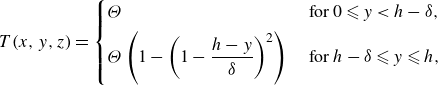 \begin{align} T(x,y,z)=\begin{cases} \Theta &\text{ for } 0\leqslant y\lt h-\delta , \\[4pt] \displaystyle \Theta \left (1-\left (1-\frac {h-y}{\delta }\right )^2\right ) &\text{ for } h-\delta \leqslant y\leqslant h, \end{cases} \end{align}
and
 $T$
defined in
$T$
defined in
 $-h\leqslant y\leqslant 0$
by symmetry. The suitability of this approximation is supported by a comparison to temperature profiles arising in the unaveraged model of Morris (Reference Morris1996), shown in figure 13(b). Since
$-h\leqslant y\leqslant 0$
by symmetry. The suitability of this approximation is supported by a comparison to temperature profiles arising in the unaveraged model of Morris (Reference Morris1996), shown in figure 13(b). Since
 $\delta$
and
$\delta$
and
 $\Theta$
are not independent, we can introduce a single variable capturing the temperature field (cf. Balmforth et al. Reference Balmforth, Craster and Sassi2004),
$\Theta$
are not independent, we can introduce a single variable capturing the temperature field (cf. Balmforth et al. Reference Balmforth, Craster and Sassi2004),
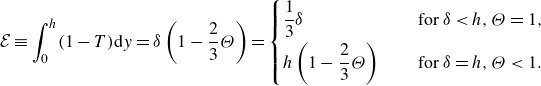 \begin{align} {\mathcal{E}}\equiv \int _0^h(1-T)\textrm {d}y=\delta \left (1-\frac {2}{3}\Theta \right )=\begin{cases} \dfrac {1}{3}\delta \quad &\text{ for } \delta \lt h, \Theta =1, \\[6pt] h\left(1-\dfrac {2}{3}\Theta \right) \quad &\text{ for } \delta = h, \Theta \lt 1. \end{cases} \end{align}
Thus, the variable
 ${\mathcal{E}}$
measures (half) the loss of dimensionless heat energy per unit area at a given point
${\mathcal{E}}$
measures (half) the loss of dimensionless heat energy per unit area at a given point
 $(x,z)$
, compared with at the inlet,
$(x,z)$
, compared with at the inlet,
 $z=0$
, and takes the value
$z=0$
, and takes the value
 $0$
when the fluid is at the hot, source temperature across the width of the channel, and the value
$0$
when the fluid is at the hot, source temperature across the width of the channel, and the value
 $h$
when the fluid is at the cooled, wall temperature across the width of the channel. We can invert the relationship (2.11) to relate
$h$
when the fluid is at the cooled, wall temperature across the width of the channel. We can invert the relationship (2.11) to relate
 $\delta$
and
$\delta$
and
 $\varTheta$
to
$\varTheta$
to
 ${\mathcal{E}}$
via
${\mathcal{E}}$
via
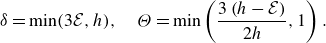 \begin{equation} \delta = \min (3{\mathcal{E}},h), \quad \Theta =\min \left (\frac {3\left (h- {\mathcal{E}}\right )}{2h},1\right ). \end{equation}
Another natural variable to define for interpretation is the cross-channel average temperature,
 ${\mathcal{T}}$
, which relates to the other variables via
${\mathcal{T}}$
, which relates to the other variables via
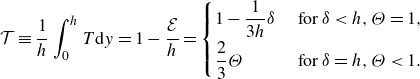 \begin{align} {\mathcal{T}}\equiv \frac {1}{h}\int _0^h T\textrm {d}y=1-\frac {{\mathcal{E}}}{h}=\begin{cases} 1-\dfrac {1}{3h}\delta & \text{ for } \delta \lt h, \Theta =1, \\[6pt] \dfrac {2}{3}\Theta & \text{ for } \delta =h, \Theta \lt 1. \end{cases} \end{align}
Integrating (2.9 b) twice, we obtain
 \begin{equation} \boldsymbol{u}_2=-\Pi \left (\int _y^h \frac {\hat {y}}{\mu (T)}\,\textrm{d}\hat {y}\right )\boldsymbol{\nabla} _2 p, \end{equation}
taking the divergence, substituting for the temperature dependent viscosity (2.5) and the temperature ansatz (2.10), and integrating over
 $-h\leqslant y\leqslant h$
gives
$-h\leqslant y\leqslant h$
gives
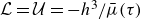
 \begin{equation} \boldsymbol{\boldsymbol{\nabla} \cdot q}\equiv 2\Pi \boldsymbol{\nabla} \boldsymbol{\cdot} \left ({\mathcal{L}}\boldsymbol{\nabla} p\right )=0, \end{equation}
where we have defined the flux,
 $\boldsymbol{q}\equiv 2\Pi {\mathcal{L}}\boldsymbol{\nabla} p$
, and we have now dropped the subscript
$\boldsymbol{q}\equiv 2\Pi {\mathcal{L}}\boldsymbol{\nabla} p$
, and we have now dropped the subscript
 $2$
from the in-plane gradient since we will consider all gradients to be in the plane of the fissure from now on. The flux factor,
$2$
from the in-plane gradient since we will consider all gradients to be in the plane of the fissure from now on. The flux factor,
 \begin{align} {\mathcal{L}}(x,z)&\equiv -\int _0^h\int _y^h\frac {\hat {y}}{\mu (T)}\,\textrm{d}\hat {y}\,\textrm{d}y \end{align}
 \begin{align}=-\delta ^3\exp (-{\gamma }(1-\Theta ))\left (\left (\frac {h}{\delta }-1\right )^2I_0+2\left (\frac {h}{\delta }-1\right )I_1+I_2+\frac {1}{3}\left (\frac {h}{\delta }-1\right )^3\right )\end{align},
where the
 $I_k$
terms are given by integrals,
$I_k$
terms are given by integrals,
 \begin{equation} I_k\equiv \int _0^1 \eta ^k\exp (-\gamma \Theta \eta ^2)\,\textrm{d}\eta , \end{equation}
which in turn can be evaluated analytically or in the form of error functions (cf. Balmforth et al. Reference Balmforth, Craster and Sassi2004). When
 $\delta \to 0$
and
$\delta \to 0$
and
 $\Theta =1$
, this reduces to
$\Theta =1$
, this reduces to
 ${\mathcal{L}}\to -h^3/3$
, which corresponds to
${\mathcal{L}}\to -h^3/3$
, which corresponds to
 $\boldsymbol{q}$
being given by Darcy’s law at the inlet viscosity
$\boldsymbol{q}$
being given by Darcy’s law at the inlet viscosity
 $\mu (1)=1$
, and when
$\mu (1)=1$
, and when
 $\delta =h$
and
$\delta =h$
and
 $\Theta =0$
, we find
$\Theta =0$
, we find
 ${\mathcal{L}}=-\exp (-\gamma )h^3/3$
, corresponding to Darcy flux at the final viscosity,
${\mathcal{L}}=-\exp (-\gamma )h^3/3$
, corresponding to Darcy flux at the final viscosity,
 $\mu (0)=\exp (\gamma )$
. Thus, the flux captures the expected results for the isothermal cases.
$\mu (0)=\exp (\gamma )$
. Thus, the flux captures the expected results for the isothermal cases.
Following Balmforth et al. (Reference Balmforth, Craster and Sassi2004), we now integrate the heat equation over the thermal boundary layer
 $h-\delta \leqslant y\leqslant h$
, obtaining a nonlinear conservation equation for
$h-\delta \leqslant y\leqslant h$
, obtaining a nonlinear conservation equation for
 ${\mathcal{E}}$
,
${\mathcal{E}}$
,
 \begin{equation} \frac {\partial {\mathcal{E}}}{\partial t}+\Pi \boldsymbol{\nabla} \cdot \left (\mathcal{S}\boldsymbol{\nabla} p\right ) = {\mathcal{C}}. \end{equation}
The right-hand side of (2.19),
 ${\mathcal{C}}\equiv 2\Theta /\delta$
, is a source term arising from cooling at the walls, while the flux of
${\mathcal{C}}\equiv 2\Theta /\delta$
, is a source term arising from cooling at the walls, while the flux of
 ${\mathcal{E}}$
,
${\mathcal{E}}$
,
 $\Pi \mathcal{S}\boldsymbol{\nabla} p$
, involves the nonlinear factor,
$\Pi \mathcal{S}\boldsymbol{\nabla} p$
, involves the nonlinear factor,
 $\mathcal{S}\equiv \mathcal{U}{\mathcal{E}}-\mathcal{G}$
, which contains a term due to advection,
$\mathcal{S}\equiv \mathcal{U}{\mathcal{E}}-\mathcal{G}$
, which contains a term due to advection,
 $\mathcal{U}{\mathcal{E}}$
, and a term arising from the vertical structure of the temperature field,
$\mathcal{U}{\mathcal{E}}$
, and a term arising from the vertical structure of the temperature field,
 $-\mathcal{G}$
. The functions
$-\mathcal{G}$
. The functions
 $\mathcal{U}$
and
$\mathcal{U}$
and
 $\mathcal{G}$
are given by
$\mathcal{G}$
are given by
 \begin{align} \mathcal{U}&=-\delta ^2\exp (-{\gamma }(1-\Theta ))\left (\left (\frac {h}{\delta }-1\right )I_1+I_2\right ), \end{align}
 \begin{align}\mathcal{G}&=-\frac {1}{3}\delta ^3\Theta \exp (-{\gamma }(1-\Theta ))\left (\left (\frac {h}{\delta }-1\right )I_1+I_2-\left (\frac {h}{\delta }-1\right )I_3-I_4\right ). \end{align}
Since we view
 $\delta$
and
$\delta$
and
 $\Theta$
as functions of
$\Theta$
as functions of
 ${\mathcal{E}}$
(via (2.12)), all of the terms
${\mathcal{E}}$
(via (2.12)), all of the terms
 ${\mathcal{L}}$
,
${\mathcal{L}}$
,
 ${\mathcal{C}}$
,
${\mathcal{C}}$
,
 $\mathcal{U}$
and
$\mathcal{U}$
and
 $\mathcal{G}$
(and hence
$\mathcal{G}$
(and hence
 $\mathcal{S}$
) are functions of
$\mathcal{S}$
) are functions of
 ${\mathcal{E}}$
(and the imposed
${\mathcal{E}}$
(and the imposed
 $h(x)$
). To summarise, we have the following system of equations for the unknown fields,
$h(x)$
). To summarise, we have the following system of equations for the unknown fields,
 ${\mathcal{E}}$
and
${\mathcal{E}}$
and
 $p$
:
$p$
:
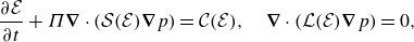 \begin{gather} \frac {\partial {\mathcal{E}}}{\partial t}+\Pi \boldsymbol{\nabla} \cdot \left (\mathcal{S}({\mathcal{E}})\boldsymbol{\nabla} p\right ) = {\mathcal{C}}({\mathcal{E}}), \quad \boldsymbol{\nabla} \cdot \left ({\mathcal{L}}({\mathcal{E}})\boldsymbol{\nabla} p\right )=0, \end{gather}
 \begin{gather} {\mathcal{C}}({\mathcal{E}})=\frac {2\Theta ({\mathcal{E}})}{\delta ({\mathcal{E}})}, \quad \delta ({\mathcal{E}}) = \min (3{\mathcal{E}},h), \quad \Theta ({\mathcal{E}})=\min \left (\frac {3\left (h- {\mathcal{E}}\right )}{2h},1\right ), \end{gather}
 \begin{gather} {\mathcal{L}}({\mathcal{E}})=-\delta ^3\exp (-{\gamma }(1-\Theta ))\left (\left (\frac {h}{\delta }-1\right )^2I_0+2\left (\frac {h}{\delta }-1\right )I_1+I_2+\frac {1}{3}\left (\frac {h}{\delta }-1\right )^3\right ), \end{gather}
 \begin{gather} \mathcal{S}({\mathcal{E}})=\mathcal{U}({\mathcal{E}}){\mathcal{E}}-\mathcal{G}({\mathcal{E}}), \quad \mathcal{U}({\mathcal{E}})=-\delta ^2\exp (-{\gamma }(1-\Theta ))\left (\left (\frac {h}{\delta }-1\right )I_1+I_2\right ), \end{gather}
 \begin{gather} \mathcal{G}({\mathcal{E}})=-\frac {1}{3}\delta ^3\Theta \exp (-{\gamma }(1-\Theta ))\left (\left (\frac {h}{\delta }-1\right )I_1+I_2-\left (\frac {h}{\delta }-1\right )I_3-I_4\right ), \end{gather}
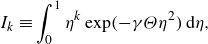 \begin{gather} I_k\equiv \int _0^1\eta ^k\exp (-\gamma \Theta \eta ^2)\,\textrm{d}\eta , \end{gather}
with boundary conditions
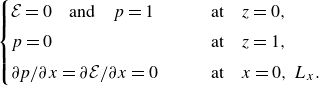 \begin{align} \begin{cases}{\mathcal{E}}=0 \quad \text{and} \quad p = 1 \quad\quad &\text{at} \quad z=0,\\[4pt] p= 0 \quad\quad &\text{at} \quad z=1, \\[4pt] \partial p/\partial x=\partial {\mathcal{E}}/{\partial x}=0 \quad\quad &\text{at} \quad x=0, \;L_x.\end{cases} \end{align}
Thus, (2.22) constitutes a nonlinear hyperbolic equation for
 ${\mathcal{E}}$
with an elliptic constraint on
${\mathcal{E}}$
with an elliptic constraint on
 $p$
. The remaining, algebraic, equations simply relate the nonlinear terms to the temperature field via
$p$
. The remaining, algebraic, equations simply relate the nonlinear terms to the temperature field via
 ${\mathcal{E}}$
. We discretise the spatial dependence of this system via a finite volume scheme, with upwinded fluxes in the
${\mathcal{E}}$
. We discretise the spatial dependence of this system via a finite volume scheme, with upwinded fluxes in the
 $z$
-direction, and we time step using a fourth-order, five-stage Rosenbrock method (Roche Reference Roche1987). Further details of the numerical method are given in Appendix A. Steady-state solutions are obtained either by natural continuation in
$z$
-direction, and we time step using a fourth-order, five-stage Rosenbrock method (Roche Reference Roche1987). Further details of the numerical method are given in Appendix A. Steady-state solutions are obtained either by natural continuation in
 $\Pi$
or by pseudo-arclength continuation. In the former, we start from a large value of
$\Pi$
or by pseudo-arclength continuation. In the former, we start from a large value of
 $\Pi$
(say
$\Pi$
(say
 $\Pi =400$
), where a temperature distribution close to the inlet temperature,
$\Pi =400$
), where a temperature distribution close to the inlet temperature,
 ${\mathcal{E}}\approx 0$
, is a good initial guess. Having obtained an initial solution, we then decrease
${\mathcal{E}}\approx 0$
, is a good initial guess. Having obtained an initial solution, we then decrease
 $\Pi$
in steps, using the previous solution as an initial guess for solving the nonlinear steady-state problem directly (i.e. by Newton iteration). If the direct solve fails, we time step to a steady state. With pseudo-arclength continuation (e.g. see Allgower & Georg Reference Allgower and Georg2003), we do not impose the step in
$\Pi$
in steps, using the previous solution as an initial guess for solving the nonlinear steady-state problem directly (i.e. by Newton iteration). If the direct solve fails, we time step to a steady state. With pseudo-arclength continuation (e.g. see Allgower & Georg Reference Allgower and Georg2003), we do not impose the step in
 $\Pi$
, but solve for a new steady state with an additional constraint that the new solution is a prescribed small distance along the solution curve from the previous one. This approach can capture fold bifurcations and unstable solution branches.
$\Pi$
, but solve for a new steady state with an additional constraint that the new solution is a prescribed small distance along the solution curve from the previous one. This approach can capture fold bifurcations and unstable solution branches.
The systems studied by Helfrich (Reference Helfrich1995) and Wylie & Lister (Reference Wylie and Lister1995) can be couched in the same manner as ours. For the Darcy averaging of Helfrich (Reference Helfrich1995), we can let
 ${\mathcal{E}}$
be instead defined by the difference between the average temperature across the fissure and the unit initial temperature, and we can set
${\mathcal{E}}$
be instead defined by the difference between the average temperature across the fissure and the unit initial temperature, and we can set
 ${\mathcal{L}}=\mathcal{U}h=-h^3/[3\mu (1-{\mathcal{E}})]$
,
${\mathcal{L}}=\mathcal{U}h=-h^3/[3\mu (1-{\mathcal{E}})]$
,
 $\mathcal{G}=0$
and
$\mathcal{G}=0$
and
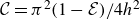 ${\mathcal{C}}=\pi ^2(1-{\mathcal{E}})/4h^2$
. For the system of Wylie & Lister (Reference Wylie and Lister1995), we let
${\mathcal{C}}=\pi ^2(1-{\mathcal{E}})/4h^2$
. For the system of Wylie & Lister (Reference Wylie and Lister1995), we let
 ${\mathcal{E}}$
represent the time-like variable they denote
${\mathcal{E}}$
represent the time-like variable they denote
 $\tau$
,
$\tau$
,
 ${\mathcal{C}}=1/h$
,
${\mathcal{C}}=1/h$
,
 $\mathcal{G}=0$
and
$\mathcal{G}=0$
and
 ${\mathcal{L}}=\mathcal{U}=-h^3/\bar {\mu }(\tau )$
, where
${\mathcal{L}}=\mathcal{U}=-h^3/\bar {\mu }(\tau )$
, where
 $\bar {\mu }(\tau )$
is an average viscosity defined by Wylie & Lister (Reference Wylie and Lister1995) and which is determined from the along-channel evolution of the full, across-channel temperature profile, requiring prior numerical evaluation. We will refer to this latter approach as the ‘unaveraged’ system, since Wylie & Lister (Reference Wylie and Lister1995) showed that it captures non-uniform steady states without approximation. Nonetheless, this system does involve an averaging over the channel and so is two-dimensional in space. As discussed by Wylie & Lister (Reference Wylie and Lister1995), the equivalence between three-dimensional and two-dimensional steady states does not carry across to time-dependent states.
$\bar {\mu }(\tau )$
is an average viscosity defined by Wylie & Lister (Reference Wylie and Lister1995) and which is determined from the along-channel evolution of the full, across-channel temperature profile, requiring prior numerical evaluation. We will refer to this latter approach as the ‘unaveraged’ system, since Wylie & Lister (Reference Wylie and Lister1995) showed that it captures non-uniform steady states without approximation. Nonetheless, this system does involve an averaging over the channel and so is two-dimensional in space. As discussed by Wylie & Lister (Reference Wylie and Lister1995), the equivalence between three-dimensional and two-dimensional steady states does not carry across to time-dependent states.
As shown in table 1, excluding the domain size,
 $L_x$
, there are essentially four parameters: the dimensionless pressure drop,
$L_x$
, there are essentially four parameters: the dimensionless pressure drop,
 $\Pi$
; the sensitivity of viscosity to temperature changes,
$\Pi$
; the sensitivity of viscosity to temperature changes,
 $\gamma$
; and the amplitude,
$\gamma$
; and the amplitude,
 $A$
, and wavelength,
$A$
, and wavelength,
 $\lambda$
, of the variations in the fissure width. As discussed by Wylie & Lister (Reference Wylie and Lister1995),
$\lambda$
, of the variations in the fissure width. As discussed by Wylie & Lister (Reference Wylie and Lister1995),
 $\Pi$
can be interpreted in a number of ways: as a dimensionless pressure drop; as a ratio of the thermal entry length to the length of the channel; or as the ratio of the characteristic rate at which heat is advected along the channel and the rate at which it is lost to the walls. Given our focus on the role of non-uniform fissure width, we largely take
$\Pi$
can be interpreted in a number of ways: as a dimensionless pressure drop; as a ratio of the thermal entry length to the length of the channel; or as the ratio of the characteristic rate at which heat is advected along the channel and the rate at which it is lost to the walls. Given our focus on the role of non-uniform fissure width, we largely take
 $\gamma$
fixed, and consider
$\gamma$
fixed, and consider
 $\Pi$
,
$\Pi$
,
 $A$
and
$A$
and
 $\lambda$
as our primary parameters. We first consider the uniform geometry (
$\lambda$
as our primary parameters. We first consider the uniform geometry (
 $A=0$
), in § 3.1, and identify the critical values of
$A=0$
), in § 3.1, and identify the critical values of
 $\gamma$
at which changes occur in the behaviour of steady-state solutions, as discussed by Helfrich (Reference Helfrich1995), Wylie & Lister (Reference Wylie and Lister1995) and Morris (Reference Morris1996). The choice of
$\gamma$
at which changes occur in the behaviour of steady-state solutions, as discussed by Helfrich (Reference Helfrich1995), Wylie & Lister (Reference Wylie and Lister1995) and Morris (Reference Morris1996). The choice of
 $\gamma =5.5$
is found to be sufficiently large that the system exhibits thermoviscous fingering and multiplicity of steady states, but not so large as to make the numerics intractable, since the numerical problem is found to become increasingly unstable with increasing
$\gamma =5.5$
is found to be sufficiently large that the system exhibits thermoviscous fingering and multiplicity of steady states, but not so large as to make the numerics intractable, since the numerical problem is found to become increasingly unstable with increasing
 $\gamma$
. This value of
$\gamma$
. This value of
 $\gamma$
corresponds to a viscosity ratio,
$\gamma$
corresponds to a viscosity ratio,
 $\mu _c/\mu _h=\exp (5.5)$
, on the order of several hundred between the source temperature and the wall temperature, which is within the range of plausible values for the volcanic application. For example, Shaw (Reference Shaw1969) suggests a value of
$\mu _c/\mu _h=\exp (5.5)$
, on the order of several hundred between the source temperature and the wall temperature, which is within the range of plausible values for the volcanic application. For example, Shaw (Reference Shaw1969) suggests a value of
 $\beta =0.1$
K
$\beta =0.1$
K
 $^{-1}$
and Spera et al. (Reference Spera, Yuen and Kirschvink1982) also suggest a value between
$^{-1}$
and Spera et al. (Reference Spera, Yuen and Kirschvink1982) also suggest a value between
 $0.02 \text{ K}^{-1}$
and
$0.02 \text{ K}^{-1}$
and
 $0.1\text{ K}^{-1}$
. Taking these two values for
$0.1\text{ K}^{-1}$
. Taking these two values for
 $\beta$
, we obtain a value of
$\beta$
, we obtain a value of
 $\gamma = 5.5$
for temperature differences,
$\gamma = 5.5$
for temperature differences,
 $T_h-T_c$
, of
$T_h-T_c$
, of
 $275\,^\circ\text{C}$
and
$275\,^\circ\text{C}$
and
 $55\,^\circ \text{C}$
, respectively.
$55\,^\circ \text{C}$
, respectively.
To explore the impact of non-uniform geometry, we then vary
 $\lambda$
between 0.2 and 20, and
$\lambda$
between 0.2 and 20, and
 $A$
between 0.01 and 0.1, solving for steady states of (2.22) over a wide range of pressure drops,
$A$
between 0.01 and 0.1, solving for steady states of (2.22) over a wide range of pressure drops,
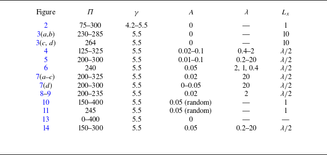
 $\Pi$
, using the numerical method detailed in Appendix A. Table 2 gives the particular values (or ranges) of the parameters used to produce each figure. We evaluate the vertical flux through the fissure,
$\Pi$
, using the numerical method detailed in Appendix A. Table 2 gives the particular values (or ranges) of the parameters used to produce each figure. We evaluate the vertical flux through the fissure,
 $q_z(x,z)=2\Pi {\mathcal{L}}\partial p/\partial z$
, which provides the total flux per unit length of the fissure,
$q_z(x,z)=2\Pi {\mathcal{L}}\partial p/\partial z$
, which provides the total flux per unit length of the fissure,
 $Q= (\int _0^{L_x} q_z \,\textrm {d}x )/L_x$
, which is independent of
$Q= (\int _0^{L_x} q_z \,\textrm {d}x )/L_x$
, which is independent of
 $z$
by conservation of mass. We also define the ratio of the maximum and minimum vertical fluxes at the surface,
$z$
by conservation of mass. We also define the ratio of the maximum and minimum vertical fluxes at the surface,
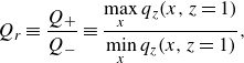 \begin{equation} Q_r\equiv \frac {Q_+}{Q_-}\equiv \frac {\displaystyle \max _{x} q_z(x,z=1)}{\displaystyle \min _x q_z(x,z=1)}, \end{equation}
which is a measure of degree of flow focussing. For comparison between sinusoidal geometries of different amplitudes, we scale this flux ratio by the value for the isothermal case (namely
 $(1+A)^3/(1-A)^3$
), defining
$(1+A)^3/(1-A)^3$
), defining
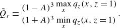 \begin{equation} \tilde {Q}_r\equiv \frac {(1-A)^3}{(1+A)^3}\frac {\displaystyle \max _x q_z(x,z=1)}{\displaystyle \min _x q_z(x,z=1)}. \end{equation}
We further evaluate the linear stability of the steady states to small perturbations. First, we revisit the uniform geometry,
 $A=0$
, and reproduce the main results of Helfrich (Reference Helfrich1995), Wylie & Lister (Reference Wylie and Lister1995) and Morris (Reference Morris1996).
$A=0$
, and reproduce the main results of Helfrich (Reference Helfrich1995), Wylie & Lister (Reference Wylie and Lister1995) and Morris (Reference Morris1996).
Values of dimensionless parameters used in each figure.
3. Results and analysis
3.1. Uniform geometry
Figure 2 shows the dimensionless flux per unit length,
 $Q$
, as a function of the dimensionless pressure drop,
$Q$
, as a function of the dimensionless pressure drop,
 $\Pi$
, for planar (i.e. independent of
$\Pi$
, for planar (i.e. independent of
 $x$
) steady-state solutions in the uniform geometry,
$x$
) steady-state solutions in the uniform geometry,
 $h=1$
, calculated using pseudo-arclength continuation. Here, we vary the value of the parameter governing the viscosity contrast,
$h=1$
, calculated using pseudo-arclength continuation. Here, we vary the value of the parameter governing the viscosity contrast,
 $\gamma =\log (\mu _c/\mu _h)$
. In the following discussion, we report the quantitative results of the current model system, while a direct comparison to the corresponding values obtained from the models of Wylie & Lister (Reference Wylie and Lister1995), Helfrich (Reference Helfrich1995) and Morris (Reference Morris1996) is given in Appendix B. The qualitative behaviour of the system is identical to that of the models in these previous studies. Namely, at low values of the viscosity contrast, the solution curve is single-valued and the planar steady states are stable. Above a first critical value,
$\gamma =\log (\mu _c/\mu _h)$
. In the following discussion, we report the quantitative results of the current model system, while a direct comparison to the corresponding values obtained from the models of Wylie & Lister (Reference Wylie and Lister1995), Helfrich (Reference Helfrich1995) and Morris (Reference Morris1996) is given in Appendix B. The qualitative behaviour of the system is identical to that of the models in these previous studies. Namely, at low values of the viscosity contrast, the solution curve is single-valued and the planar steady states are stable. Above a first critical value,
 $\gamma _c=4.8$
, the curve becomes multivalued, resulting in three branches of the solution curve: a ‘hot’, fast branch at high pressure drops; a ‘cold’, slow branch at low pressure drops; and an intermediate branch on which the flux increases with decreasing pressure drop. As in previous studies, the intermediate branch is found to be unstable to a planar instability (i.e. to perturbations with vanishing wavenumber in the
$\gamma _c=4.8$
, the curve becomes multivalued, resulting in three branches of the solution curve: a ‘hot’, fast branch at high pressure drops; a ‘cold’, slow branch at low pressure drops; and an intermediate branch on which the flux increases with decreasing pressure drop. As in previous studies, the intermediate branch is found to be unstable to a planar instability (i.e. to perturbations with vanishing wavenumber in the
 $x$
-direction), which acts to drive solutions off the intermediate branch and towards the fast or slow branches of the solution curve. Above a second, higher, viscosity ratio,
$x$
-direction), which acts to drive solutions off the intermediate branch and towards the fast or slow branches of the solution curve. Above a second, higher, viscosity ratio,
 $\gamma _{3d}\approx 5.2$
, there exist solutions which are most unstable to perturbations with non-vanishing wavenumber in the
$\gamma _{3d}\approx 5.2$
, there exist solutions which are most unstable to perturbations with non-vanishing wavenumber in the
 $x$
-direction (see the dotted region of the solution curves for
$x$
-direction (see the dotted region of the solution curves for
 $\gamma =5.37$
and
$\gamma =5.37$
and
 $\gamma =5.5$
in figure 2). This thus marks the onset of a fingering instability, analogous to classical Saffmann–Taylor viscous fingering, by which the uniform steady states go unstable to the formation of alternating regions of hot, low-viscosity fluid, and cold, high-viscosity fluid. At
$\gamma =5.5$
in figure 2). This thus marks the onset of a fingering instability, analogous to classical Saffmann–Taylor viscous fingering, by which the uniform steady states go unstable to the formation of alternating regions of hot, low-viscosity fluid, and cold, high-viscosity fluid. At
 $\gamma$
just above
$\gamma$
just above
 $\gamma _{3d}$
, the region of the solution curve which is most unstable to the fingering instability is limited to a small region near the fold bifurcation that joins the slow and intermediate solution branches. As
$\gamma _{3d}$
, the region of the solution curve which is most unstable to the fingering instability is limited to a small region near the fold bifurcation that joins the slow and intermediate solution branches. As
 $\gamma$
is increased further, this region extends down the slow solution branch and the entire slow branch becomes unstable to the fingering instability at a third critical value of the viscosity ratio,
$\gamma$
is increased further, this region extends down the slow solution branch and the entire slow branch becomes unstable to the fingering instability at a third critical value of the viscosity ratio,
 $\gamma _\infty \approx 5.4$
. Thus, by
$\gamma _\infty \approx 5.4$
. Thus, by
 $\gamma =5.5$
, the entire slow branch is unstable to the fingering instability and, as we will discuss later, we are able to find stable non-planar steady states reached after the onset of fingering. We report approximate values of
$\gamma =5.5$
, the entire slow branch is unstable to the fingering instability and, as we will discuss later, we are able to find stable non-planar steady states reached after the onset of fingering. We report approximate values of
 $\gamma _{3d}$
and
$\gamma _{3d}$
and
 $\gamma _\infty$
here, because these results were calculated using our numerical method, with a finite domain (
$\gamma _\infty$
here, because these results were calculated using our numerical method, with a finite domain (
 $L_x=1$
in the cases shown in figure 2) and symmetry boundary conditions. This does not affect the calculation of
$L_x=1$
in the cases shown in figure 2) and symmetry boundary conditions. This does not affect the calculation of
 $Q$
for the planar steady states, nor the stability of the solutions to the planar instability; however, it does impact the stability to non-planar perturbations, since the finite domain restricts perturbations to those fitting inside the domain (with a half-integer number of wavelengths). Thus, for an infinite domain,
$Q$
for the planar steady states, nor the stability of the solutions to the planar instability; however, it does impact the stability to non-planar perturbations, since the finite domain restricts perturbations to those fitting inside the domain (with a half-integer number of wavelengths). Thus, for an infinite domain,
 $\gamma _{3d}$
is likely slightly smaller than reported here. Similarly, the finite resolution of the grid sets a lower bound on the wavelengths that can be accurately captured. Since the wavelength of the most unstable mode decreases with decreasing
$\gamma _{3d}$
is likely slightly smaller than reported here. Similarly, the finite resolution of the grid sets a lower bound on the wavelengths that can be accurately captured. Since the wavelength of the most unstable mode decreases with decreasing
 $\Pi$
(see later and Wylie & Lister Reference Wylie and Lister1995; Morris Reference Morris1996), determining
$\Pi$
(see later and Wylie & Lister Reference Wylie and Lister1995; Morris Reference Morris1996), determining
 $\gamma _\infty$
(where the fingering instability first extends to arbitrarily small values of
$\gamma _\infty$
(where the fingering instability first extends to arbitrarily small values of
 $\Pi$
) is difficult with our numerical method. Ultimately, our aim is to study the impact of a spatially varying channel width at a fixed value of
$\Pi$
) is difficult with our numerical method. Ultimately, our aim is to study the impact of a spatially varying channel width at a fixed value of
 $\gamma$
and moderate values of
$\gamma$
and moderate values of
 $\Pi$
(in the neighbourhood of the fold bifurcation), and not to accurately capture these critical values of
$\Pi$
(in the neighbourhood of the fold bifurcation), and not to accurately capture these critical values of
 $\gamma$
for an infinite uniform geometry.
$\gamma$
for an infinite uniform geometry.
Dimensionless flux per unit length,
 $Q$
, against dimensionless pressure drop,
$Q$
, against dimensionless pressure drop,
 $\Pi \equiv \Delta p h_0^4/\kappa \mu _h L^2$
, for planar steady states in the uniform geometry,
$\Pi \equiv \Delta p h_0^4/\kappa \mu _h L^2$
, for planar steady states in the uniform geometry,
 $h=1$
. Results are shown for several values of
$h=1$
. Results are shown for several values of
 $\gamma =\log (\mu _c/\mu _h)$
. The dimensional flux per metre is given by
$\gamma =\log (\mu _c/\mu _h)$
. The dimensional flux per metre is given by
 $\kappa L Q/h_0$
. Solid lines show stable regions of the solution curve, and dashed and dotted lines show regions that are most unstable to planar and non-planar perturbations, respectively. See table 2 for other parameters used in these solutions.
$\kappa L Q/h_0$
. Solid lines show stable regions of the solution curve, and dashed and dotted lines show regions that are most unstable to planar and non-planar perturbations, respectively. See table 2 for other parameters used in these solutions.
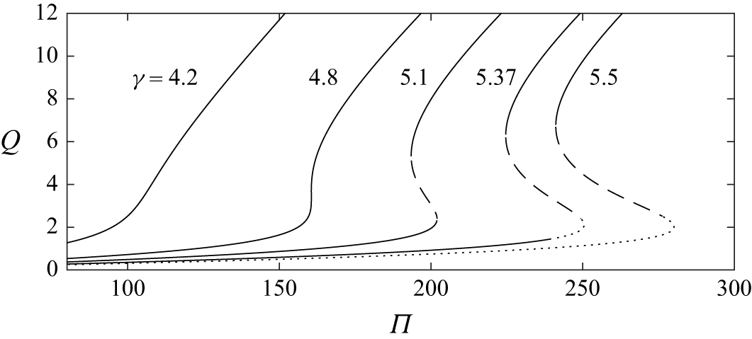
We now provide some more detail of the steady-state solutions for the uniform geometry,
 $h=1$
, and at
$h=1$
, and at
 $\gamma =5.5$
, fixed (now on a larger domain,
$\gamma =5.5$
, fixed (now on a larger domain,
 $L_x=10$
). Figure 3(a) again shows the total flux per unit length of the fissure,
$L_x=10$
). Figure 3(a) again shows the total flux per unit length of the fissure,
 $Q$
, as a function of
$Q$
, as a function of
 $\Pi$
at steady state. The black (solid, dashed and dotted) line shows the solution branch for the planar solutions (independent of
$\Pi$
at steady state. The black (solid, dashed and dotted) line shows the solution branch for the planar solutions (independent of
 $x$
), as in figure 2. Point A indicates the fold bifurcation, below which the planar steady states are unstable. The wavenumber,
$x$
), as in figure 2. Point A indicates the fold bifurcation, below which the planar steady states are unstable. The wavenumber,
 $k$
, of the most unstable mode for the unique planar steady state with flux,
$k$
, of the most unstable mode for the unique planar steady state with flux,
 $Q$
, is shown in figure 3(b). In panels (a) and (b), point B indicates the location at which the most unstable mode becomes non-planar (
$Q$
, is shown in figure 3(b). In panels (a) and (b), point B indicates the location at which the most unstable mode becomes non-planar (
 $k\neq 0$
). Assuming the eruption starts at a high pressure drop and wanes with time, the structure of the bifurcation diagram gives the potential for the system to pass through the fold bifurcation and exhibit a sudden reduction in flux before localising due to the fingering instability. As reported by Wylie & Lister (Reference Wylie and Lister1995) and Morris (Reference Morris1996), the wavenumber of the most unstable mode increases as
$k\neq 0$
). Assuming the eruption starts at a high pressure drop and wanes with time, the structure of the bifurcation diagram gives the potential for the system to pass through the fold bifurcation and exhibit a sudden reduction in flux before localising due to the fingering instability. As reported by Wylie & Lister (Reference Wylie and Lister1995) and Morris (Reference Morris1996), the wavenumber of the most unstable mode increases as
 $\Pi$
decreases, and scales with
$\Pi$
decreases, and scales with
 $1/Q$
(see the red dashed curve in figure 3
b) since the length scale is set by the thermal entry length. For our results, the wavenumber curve in figure 3(b) is stepped, which is simply the signature of the finite domain (in this case,
$1/Q$
(see the red dashed curve in figure 3
b) since the length scale is set by the thermal entry length. For our results, the wavenumber curve in figure 3(b) is stepped, which is simply the signature of the finite domain (in this case,
 $L_x=10$
) and symmetry boundary conditions, meaning that the wavenumers can only take half-integer multiples of
$L_x=10$
) and symmetry boundary conditions, meaning that the wavenumers can only take half-integer multiples of
 $1/L_x$
– however, by taking the domain size to infinity, we could retrieve a perfectly continuous spectrum of wavenumbers.
$1/L_x$
– however, by taking the domain size to infinity, we could retrieve a perfectly continuous spectrum of wavenumbers.
(a) Dimensionless flux per unit length of the fissure,
 $Q$
, as a function of dimensionless pressure drop,
$Q$
, as a function of dimensionless pressure drop,
 $\Pi$
, for stable steady states with
$\Pi$
, for stable steady states with
 $h=1$
and
$h=1$
and
 $\gamma =5.5$
(as in figure 2). The colour indicates the surface flux ratio,
$\gamma =5.5$
(as in figure 2). The colour indicates the surface flux ratio,
 $Q_r$
defined by (2.29), and the planar steady-state solution curve is shown by the black dashed and dotted line. Point A shows the fold bifurcation at which the solutions go unstable to planar perturbations, and point B indicates the location at which the solutions become most unstable to non-planar perturbations. (b) Wavenumber of the most unstable mode,
$Q_r$
defined by (2.29), and the planar steady-state solution curve is shown by the black dashed and dotted line. Point A shows the fold bifurcation at which the solutions go unstable to planar perturbations, and point B indicates the location at which the solutions become most unstable to non-planar perturbations. (b) Wavenumber of the most unstable mode,
 $k$
, as a function of
$k$
, as a function of
 $Q$
(black). The red dashed line shows a curve proportional to
$Q$
(black). The red dashed line shows a curve proportional to
 $1/Q$
. Points A and B as in panel (a). (c) Dimensionless cross-fissure average temperature,
$1/Q$
. Points A and B as in panel (a). (c) Dimensionless cross-fissure average temperature,
 ${\mathcal{T}}$
defined in (2.13), for the last stable steady state near the slow branch at
${\mathcal{T}}$
defined in (2.13), for the last stable steady state near the slow branch at
 $\Pi =264$
. The domain has been reduced to show a single wavelength of the fingering pattern (of wavelength
$\Pi =264$
. The domain has been reduced to show a single wavelength of the fingering pattern (of wavelength
 $0.909$
). The contours are plotted from
$0.909$
). The contours are plotted from
 ${\mathcal{T}}=0.1$
near the top and increase in increments of 0.1. (d) Contour plot of vertical flux,
${\mathcal{T}}=0.1$
near the top and increase in increments of 0.1. (d) Contour plot of vertical flux,
 $q_z=2\Pi {\mathcal{L}}\partial p/\partial z$
, for the solution shown in panel (c). The central (closed) contour is for
$q_z=2\Pi {\mathcal{L}}\partial p/\partial z$
, for the solution shown in panel (c). The central (closed) contour is for
 $q_z=2.4$
, and values decrease in increments of 0.2 moving out from here. Note that the results in
$q_z=2.4$
, and values decrease in increments of 0.2 moving out from here. Note that the results in
 $x\lt 0$
have been produced by reflecting in
$x\lt 0$
have been produced by reflecting in
 $x=0$
and have not been explicitly calculated. See table 2 for other parameters used in these solutions.
$x=0$
and have not been explicitly calculated. See table 2 for other parameters used in these solutions.
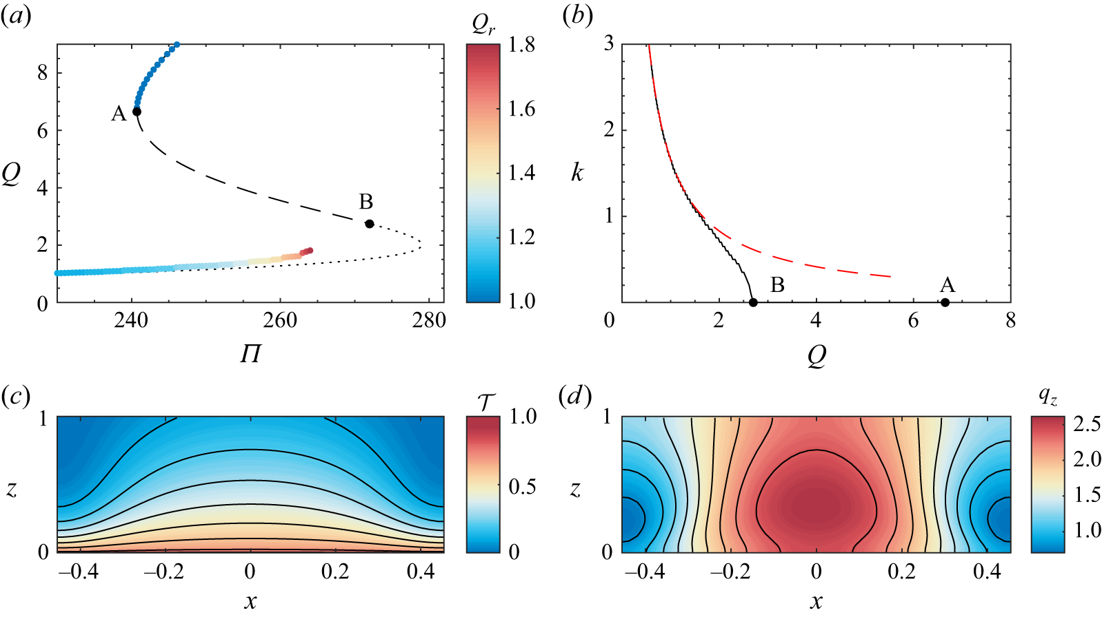
Figure 3(a) also shows coloured points representing stable steady states. As noted previously, the fast branch of the planar solutions is stable. The stable solutions near the slow branch were obtained by natural continuation, starting at
 $\Pi =200$
and increasing
$\Pi =200$
and increasing
 $\Pi$
in steps of 0.5. At each step, the new steady state is either stable, in which case, it is kept; or else, it is unstable, in which case, it is perturbed by its most unstable perturbation and evolved forwards in time until a new steady state is reached. The colour is set by the surface flux ratio,
$\Pi$
in steps of 0.5. At each step, the new steady state is either stable, in which case, it is kept; or else, it is unstable, in which case, it is perturbed by its most unstable perturbation and evolved forwards in time until a new steady state is reached. The colour is set by the surface flux ratio,
 $Q_r$
, defined by (2.29). Thus,
$Q_r$
, defined by (2.29). Thus,
 $Q_r=1$
on the fast, planar branch, and
$Q_r=1$
on the fast, planar branch, and
 $Q_r\gt 1$
near the slow branch where there are flow-focussed regions. We found that at values of
$Q_r\gt 1$
near the slow branch where there are flow-focussed regions. We found that at values of
 $\Pi$
close to the onset of the non-planar instability (point B in figure 3), the perturbed solutions evolve onto the fast branch of the solution curve, resulting in no non-planar steady states, as was observed by Wylie & Lister (Reference Wylie and Lister1995) when trying to find non-planar steady states. However, at lower
$\Pi$
close to the onset of the non-planar instability (point B in figure 3), the perturbed solutions evolve onto the fast branch of the solution curve, resulting in no non-planar steady states, as was observed by Wylie & Lister (Reference Wylie and Lister1995) when trying to find non-planar steady states. However, at lower
 $\Pi$
, we find that the non-planar solutions evolve towards stable steady states with localised finger regions, as suggested by the solutions of Helfrich (Reference Helfrich1995). This result was also reproduced for the unaveraged system of Wylie & Lister (Reference Wylie and Lister1995), but at a higher viscosity ratio,
$\Pi$
, we find that the non-planar solutions evolve towards stable steady states with localised finger regions, as suggested by the solutions of Helfrich (Reference Helfrich1995). This result was also reproduced for the unaveraged system of Wylie & Lister (Reference Wylie and Lister1995), but at a higher viscosity ratio,
 $\gamma =6\gt \gamma _\infty$
, such that the entire slow branch is unstable to the fingering instability. The total flux of these flow-focussed states is slightly increased compared with the unstable steady state, and is distributed into higher and lower flux regions along the fissure. Among these solutions, the surface flux ratio and the wavelength of the finite amplitude fingering pattern both increase with
$\gamma =6\gt \gamma _\infty$
, such that the entire slow branch is unstable to the fingering instability. The total flux of these flow-focussed states is slightly increased compared with the unstable steady state, and is distributed into higher and lower flux regions along the fissure. Among these solutions, the surface flux ratio and the wavelength of the finite amplitude fingering pattern both increase with
 $\Pi$
, reaching a maximum surface flux ratio of
$\Pi$
, reaching a maximum surface flux ratio of
 $Q_r\approx 1.8$
at the last pressure drop before the non-planar solutions become unstable and instead evolve onto the fast branch (in this case,
$Q_r\approx 1.8$
at the last pressure drop before the non-planar solutions become unstable and instead evolve onto the fast branch (in this case,
 $\Pi =264$
). We again note that on this steady flow-focussed branch, the finite domain size and symmetry boundary conditions are relevant, since only a half-integer number of wavelengths can fit in the domain. Thus, the increase of the wavelength with increasing
$\Pi =264$
). We again note that on this steady flow-focussed branch, the finite domain size and symmetry boundary conditions are relevant, since only a half-integer number of wavelengths can fit in the domain. Thus, the increase of the wavelength with increasing
 $\Pi$
does not occur continuously, but in discrete jumps marked by a sequence of bifurcations. Indeed, since the solutions are calculated by natural continuation, figure 3(a) does not capture all stable steady-state branches; rather, there is a separate solution branch corresponding to each half-integer number of fingers within the domain, and the regions over which each branch is stable are overlapping. Thus, in figure 3(a), we follow a branch up to the
$\Pi$
does not occur continuously, but in discrete jumps marked by a sequence of bifurcations. Indeed, since the solutions are calculated by natural continuation, figure 3(a) does not capture all stable steady-state branches; rather, there is a separate solution branch corresponding to each half-integer number of fingers within the domain, and the regions over which each branch is stable are overlapping. Thus, in figure 3(a), we follow a branch up to the
 $\Pi$
at which it goes unstable, and then land on the next stable branch which is again captured up until the
$\Pi$
at which it goes unstable, and then land on the next stable branch which is again captured up until the
 $\Pi$
at which it goes unstable, and so on. The bifurcation which results in the onset of instability on one branch, and the transition to the next, is a subcritical pitchfork bifurcation (e.g. see Strogatz Reference Strogatz2015a
), involving the symmetry-breaking selection of which end of the domain switches from a hot to a cold finger (or vice versa). In contrast, for an infinite domain,
$\Pi$
at which it goes unstable, and so on. The bifurcation which results in the onset of instability on one branch, and the transition to the next, is a subcritical pitchfork bifurcation (e.g. see Strogatz Reference Strogatz2015a
), involving the symmetry-breaking selection of which end of the domain switches from a hot to a cold finger (or vice versa). In contrast, for an infinite domain,
 $L_x=\infty$
, we would anticipate that the flow-focussed steady-state branch would be a single continuous curve with a continually varying wavelength.
$L_x=\infty$
, we would anticipate that the flow-focussed steady-state branch would be a single continuous curve with a continually varying wavelength.
Figure 3(c,d) shows contour plots of the cross-channel average temperature,
 ${\mathcal{T}}$
, and vertical flux,
${\mathcal{T}}$
, and vertical flux,
 $q_z$
, for the final stable steady solution on the non-planar steady-state curve at
$q_z$
, for the final stable steady solution on the non-planar steady-state curve at
 $\Pi =264$
, evidencing a finger structure with a wavenumber of
$\Pi =264$
, evidencing a finger structure with a wavenumber of
 $k=1.1$
(i.e. 11 wavelengths in the domain of width
$k=1.1$
(i.e. 11 wavelengths in the domain of width
 $L_x=10$
), which is close to the most unstable wavenumber,
$L_x=10$
), which is close to the most unstable wavenumber,
 $k=1.2$
, predicted for the uniform steady state at the same pressure drop. This figure also demonstrates why the ratio of fluxes at the surfaces,
$k=1.2$
, predicted for the uniform steady state at the same pressure drop. This figure also demonstrates why the ratio of fluxes at the surfaces,
 $Q_r=1.8$
, is not particularly large (compared with values obtained for the non-uniform geometry discussed later, see § 3.2), since the localisation occurs most significantly at depth before becoming more uniform nearer the surface where the magma is close to the wall temperature,
$Q_r=1.8$
, is not particularly large (compared with values obtained for the non-uniform geometry discussed later, see § 3.2), since the localisation occurs most significantly at depth before becoming more uniform nearer the surface where the magma is close to the wall temperature,
 $T=0$
. Under the model of a waning eruptive pressure drop (and assuming that the pressure drop varies sufficiently gradually that the system progresses through steady states), the system would drop off the fast branch at the fold bifurcaton around
$T=0$
. Under the model of a waning eruptive pressure drop (and assuming that the pressure drop varies sufficiently gradually that the system progresses through steady states), the system would drop off the fast branch at the fold bifurcaton around
 $\Pi =240$
and first attain a non-planar solution at this value. In this case, the surface flux ratio would be smaller, resulting in a
$\Pi =240$
and first attain a non-planar solution at this value. In this case, the surface flux ratio would be smaller, resulting in a
 $14\,\%$
difference in flux between the hot and cold regions of the outflow. It should be noted that at
$14\,\%$
difference in flux between the hot and cold regions of the outflow. It should be noted that at
 $\gamma =5.5$
, we are not particularly far above the onset of the fingering instability (at
$\gamma =5.5$
, we are not particularly far above the onset of the fingering instability (at
 $\gamma _{3d}\approx 5.2$
), and one would anticipate that at larger viscosity ratios, the steady-state fingered solutions would exhibit a greater degree of flow-focussing. This will also be true of the geometrically flow-focussed states, discussed in the following sections, and which we will show are associated with the fold instability arising first at
$\gamma _{3d}\approx 5.2$
), and one would anticipate that at larger viscosity ratios, the steady-state fingered solutions would exhibit a greater degree of flow-focussing. This will also be true of the geometrically flow-focussed states, discussed in the following sections, and which we will show are associated with the fold instability arising first at
 $\gamma _c=4.8$
.
$\gamma _c=4.8$
.
In this section, we have revisited the uniform geometry case, and shown that our results provide close qualitative agreement with the previous findings of Helfrich (Reference Helfrich1995), Wylie & Lister (Reference Wylie and Lister1995) and Morris (Reference Morris1996), evidencing multiple steady states and the onset of the thermoviscous fingering instability at low pressure drops. Crucially, these results provide the baseline case against which to interpret the results in the non-uniform geometry, which we consider next. A quantitative comparison to the alternative averaging approaches of Helfrich (Reference Helfrich1995), Wylie & Lister (Reference Wylie and Lister1995) and Morris (Reference Morris1996) is made in Appendix B, showing that the heat balance averaging of § 2.1 improves on the averaging of Helfrich (Reference Helfrich1995), but that there are nonetheless quantitative discrepancies with the unaveraged system. We note that there are multiple other approximations that are likely to have equally significant effects on the quantitative predictions of all models, in particular, the simple treatment of the thermodynamics at the fissure walls and the particular choice of the viscosity function, (2.5). For example, results of Wylie & Lister (Reference Wylie and Lister1995, p. 248) employing a step-function model for the viscosity find a critical viscosity ratio,
 $\mu _c/\mu _h$
, an order of magnitude smaller than when employing the exponential viscosity model (12 compared with 190), and Morris (Reference Morris1996, p. 126) finds a critical viscosity ratio of just 7.3 when the temperature of the fissure walls vary linearly with flow direction. In using the heat balance averaging detailed in § 2.1, we thus accept an additional source of approximation and associated quantitative discrepancy with the unaveraged system, in exchange for a number of advantages. As noted before, in employing the heat balance averaging, we consistently average the time derivative in the heat equation, meaning that time-dependent states (for example, those discussed in §§ 3.4 and 4) can be meaningfully considered alongside the steady states of the system – with both arising from the same assumed structure of the temperature profile and resulting average of the heat equation. Second, from a purely practical standpoint, in the unaveraged approach, evaluation of the functions
$\mu _c/\mu _h$
, an order of magnitude smaller than when employing the exponential viscosity model (12 compared with 190), and Morris (Reference Morris1996, p. 126) finds a critical viscosity ratio of just 7.3 when the temperature of the fissure walls vary linearly with flow direction. In using the heat balance averaging detailed in § 2.1, we thus accept an additional source of approximation and associated quantitative discrepancy with the unaveraged system, in exchange for a number of advantages. As noted before, in employing the heat balance averaging, we consistently average the time derivative in the heat equation, meaning that time-dependent states (for example, those discussed in §§ 3.4 and 4) can be meaningfully considered alongside the steady states of the system – with both arising from the same assumed structure of the temperature profile and resulting average of the heat equation. Second, from a purely practical standpoint, in the unaveraged approach, evaluation of the functions
 ${\mathcal{L}}$
and
${\mathcal{L}}$
and
 $\mathcal{S}$
, and their derivatives, relies on interpolation and numerical differentiation of a precomputed table of values,
$\mathcal{S}$
, and their derivatives, relies on interpolation and numerical differentiation of a precomputed table of values,
 $\bar {\mu }(\tau )$
. Furthermore, the derivative
$\bar {\mu }(\tau )$
. Furthermore, the derivative
 $\textrm {d}{\mathcal{L}}/\textrm {d}\tau$
diverges at
$\textrm {d}{\mathcal{L}}/\textrm {d}\tau$
diverges at
 $\tau =0$
. These features make the numerical solution of the resulting equations harder than when employing the analytical expressions for
$\tau =0$
. These features make the numerical solution of the resulting equations harder than when employing the analytical expressions for
 ${\mathcal{L}}$
and
${\mathcal{L}}$
and
 $\mathcal{S}$
arising from the heat balance averaging.
$\mathcal{S}$
arising from the heat balance averaging.
Steady-state solution curves for different amplitudes and wavelengths of the dimensionless fissure half-width,
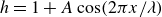 $h=1+A\cos (2\pi x/\lambda )$
. Each panel shows average flux per unit length,
$h=1+A\cos (2\pi x/\lambda )$
. Each panel shows average flux per unit length,
 $Q$
, as a function of the dimensionless pressure drop,
$Q$
, as a function of the dimensionless pressure drop,
 $\Pi$
, as in figure 2, with points coloured by the scaled surface flux ratio,
$\Pi$
, as in figure 2, with points coloured by the scaled surface flux ratio,
 $\tilde {Q}_r$
, defined by (2.30) (note the logarithmic colour scale). The wavelength,
$\tilde {Q}_r$
, defined by (2.30) (note the logarithmic colour scale). The wavelength,
 $\lambda$
, is shown in the title and the three coloured curves correspond to amplitudes of
$\lambda$
, is shown in the title and the three coloured curves correspond to amplitudes of
 $A=0.02$
,
$A=0.02$
,
 $0.05$
and
$0.05$
and
 $0.1$
(increasing in the direction shown). The solution curve for the planar steady states in the uniform geometry (
$0.1$
(increasing in the direction shown). The solution curve for the planar steady states in the uniform geometry (
 $A=0$
) is shown as the black dotted curve in all panels. See table 2 for other parameters used in these solutions.
$A=0$
) is shown as the black dotted curve in all panels. See table 2 for other parameters used in these solutions.
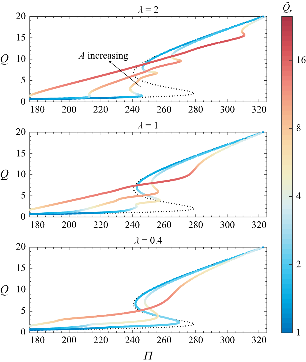
Colour plot of scaled surface flux ratio,
 $\tilde {Q}_r$
(2.30), as a function of dimensionless pressure drop,
$\tilde {Q}_r$
(2.30), as a function of dimensionless pressure drop,
 $\Pi$
, and the wavelength of the variations in width,
$\Pi$
, and the wavelength of the variations in width,
 $\lambda$
, at different values of the amplitude,
$\lambda$
, at different values of the amplitude,
 $A$
. Contours (black) are plotted at flux ratios of
$A$
. Contours (black) are plotted at flux ratios of
 $\tilde {Q}_r=4$
and 8 in all panels, and at the additional level
$\tilde {Q}_r=4$
and 8 in all panels, and at the additional level
 $\tilde {Q}_r=16$
, in panel (d). The axis ticks indicate the location of solutions used to construct the contour plot, and red dots indicate that an average over the period of a periodic solution was used as opposed to a steady-state solution. Note the extended
$\tilde {Q}_r=16$
, in panel (d). The axis ticks indicate the location of solutions used to construct the contour plot, and red dots indicate that an average over the period of a periodic solution was used as opposed to a steady-state solution. Note the extended
 $\Pi$
-axis in the final panel. See table 2 for other parameters used in these solutions.
$\Pi$
-axis in the final panel. See table 2 for other parameters used in these solutions.
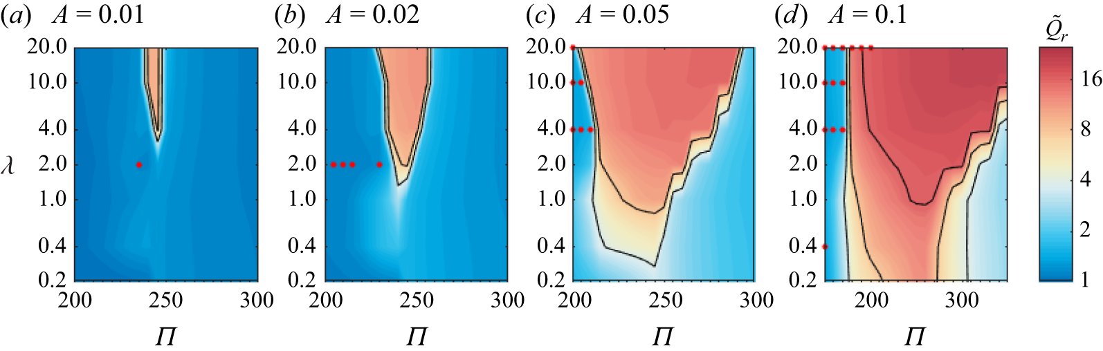
3.2. Non-uniform geometry
We now introduce a sinusoidal perturbation to the fissure width, at different amplitudes and wavelengths. Figure 4 shows the corresponding
 $Q\! (\Pi )$
steady-state solution curves for
$Q\! (\Pi )$
steady-state solution curves for
 $\lambda =0.4, 1$
and
$\lambda =0.4, 1$
and
 $2$
, and
$2$
, and
 $A=0.02, 0.05$
and
$A=0.02, 0.05$
and
 $0.1$
. The solution curve corresponding to the planar solutions of the uniform geometry (
$0.1$
. The solution curve corresponding to the planar solutions of the uniform geometry (
 $A=0$
) is shown as a dashed line and the colours now indicate the scaled surface flux ratio,
$A=0$
) is shown as a dashed line and the colours now indicate the scaled surface flux ratio,
 $\tilde {Q}_r$
defined by (2.30). We also now use a logarithmic scale for the colour bar. We see that the effect of the non-uniform geometry is generally to replace the unstable intermediate branch of the planar solutions with a stable solution branch, exhibiting significant flux focussing. This stable, ‘focussed’, branch is either part of a continuous single-valued solution curve, or is connected to the original fast and/or slow branches by one or two pairs of fold bifurcations (for example, for
$\tilde {Q}_r$
defined by (2.30). We also now use a logarithmic scale for the colour bar. We see that the effect of the non-uniform geometry is generally to replace the unstable intermediate branch of the planar solutions with a stable solution branch, exhibiting significant flux focussing. This stable, ‘focussed’, branch is either part of a continuous single-valued solution curve, or is connected to the original fast and/or slow branches by one or two pairs of fold bifurcations (for example, for
 $A=0.05$
and
$A=0.05$
and
 $\lambda =2$
, there are two pairs of fold bifurcations, one at either end of the stable central branch). The deviation from the uniform geometry solution increases with both amplitude and wavelength. Further results for the scaled surface flux ratio,
$\lambda =2$
, there are two pairs of fold bifurcations, one at either end of the stable central branch). The deviation from the uniform geometry solution increases with both amplitude and wavelength. Further results for the scaled surface flux ratio,
 $\tilde {Q}_r$
, are shown for a wider range of wavelengths and amplitudes in figure 5. For this plot, the solutions were found by natural continuation in the pressure drop,
$\tilde {Q}_r$
, are shown for a wider range of wavelengths and amplitudes in figure 5. For this plot, the solutions were found by natural continuation in the pressure drop,
 $\Pi$
, starting on the fast branch with
$\Pi$
, starting on the fast branch with
 $\Pi =400$
and integrating forwards in time to obtain stable steady states as
$\Pi =400$
and integrating forwards in time to obtain stable steady states as
 $\Pi$
is decreased in discrete steps. This clearly evidences the existence of the highly localised solutions at intermediate pressure drops, and the dependence on the wavelength and amplitude of the fissure geometry. There are a small number of parameter values, primarily lying on the slow solution branch, at which no steady state was found (indicated by red dots in figure 5), and the solutions were instead found to be periodic. Oscillatory dynamics have previously been observed by Pailha et al. (Reference Pailha, Hazel, Glendinning and Juel2012) in experiments on isothermal fingers of air displacing viscous fluids, where geometrical constraints were found to play a key role (see also Thompson, Juel & Hazel Reference Thompson, Juel and Hazel2014; Franco-Gómez et al. Reference Franco-Gómez, Thompson, Hazel and Juel2016; Lawless, Hazel & Juel Reference Lawless, Hazel and Juel2024). The structure of the periodic solutions observed in these cases is rather different from those observed here. We explore the periodic solutions in more detail in § 3.4, but note that since these have a period-averaged surface flux ratio in line with neighbouring steady solutions (see figure 5), the implication for the degree of fissure localisation is minimal. The temperature and flux distributions are shown in figure 6 for steady-state solutions at
$\Pi$
is decreased in discrete steps. This clearly evidences the existence of the highly localised solutions at intermediate pressure drops, and the dependence on the wavelength and amplitude of the fissure geometry. There are a small number of parameter values, primarily lying on the slow solution branch, at which no steady state was found (indicated by red dots in figure 5), and the solutions were instead found to be periodic. Oscillatory dynamics have previously been observed by Pailha et al. (Reference Pailha, Hazel, Glendinning and Juel2012) in experiments on isothermal fingers of air displacing viscous fluids, where geometrical constraints were found to play a key role (see also Thompson, Juel & Hazel Reference Thompson, Juel and Hazel2014; Franco-Gómez et al. Reference Franco-Gómez, Thompson, Hazel and Juel2016; Lawless, Hazel & Juel Reference Lawless, Hazel and Juel2024). The structure of the periodic solutions observed in these cases is rather different from those observed here. We explore the periodic solutions in more detail in § 3.4, but note that since these have a period-averaged surface flux ratio in line with neighbouring steady solutions (see figure 5), the implication for the degree of fissure localisation is minimal. The temperature and flux distributions are shown in figure 6 for steady-state solutions at
 $\Pi =240$
on the focussed branch for
$\Pi =240$
on the focussed branch for
 $A=0.05$
and
$A=0.05$
and
 $\lambda =2$
, 1 and 0.5. These can be compared with figure 3(d,e) for the focussed solutions arising from thermoviscous fingering in a uniform geometry at
$\lambda =2$
, 1 and 0.5. These can be compared with figure 3(d,e) for the focussed solutions arising from thermoviscous fingering in a uniform geometry at
 $\Pi =264$
, showing that the temperature variations penetrate further up the fissure and that the vertical flux variations are several times larger.
$\Pi =264$
, showing that the temperature variations penetrate further up the fissure and that the vertical flux variations are several times larger.
(a) Cross-channel average temperature,
 ${\mathcal{T}}$
, defined in (2.13), for steady-state solutions at
${\mathcal{T}}$
, defined in (2.13), for steady-state solutions at
 $\Pi =240$
with
$\Pi =240$
with
 $A=0.05$
and
$A=0.05$
and
 $\lambda =2,\,1,\,0.4$
(from left to right). The colour bar is shared between panels, and the contours are plotted from
$\lambda =2,\,1,\,0.4$
(from left to right). The colour bar is shared between panels, and the contours are plotted from
 ${\mathcal{T}}=0.1$
near the top left/right and increase in increments of 0.1. (b) Vertical flux,
${\mathcal{T}}=0.1$
near the top left/right and increase in increments of 0.1. (b) Vertical flux,
 $q_z\equiv 2{\mathcal{L}}\partial p/\partial z$
, for the same solutions. Contours are plotted from
$q_z\equiv 2{\mathcal{L}}\partial p/\partial z$
, for the same solutions. Contours are plotted from
 $q_z=2$
at the left and right, and increase inwards in increments of 2. Note that the results in
$q_z=2$
at the left and right, and increase inwards in increments of 2. Note that the results in
 $x\lt 0$
have been produced by reflecting in
$x\lt 0$
have been produced by reflecting in
 $x=0$
, and have not been explicitly calculated. See table 2 for other parameters used in these solutions.
$x=0$
, and have not been explicitly calculated. See table 2 for other parameters used in these solutions.
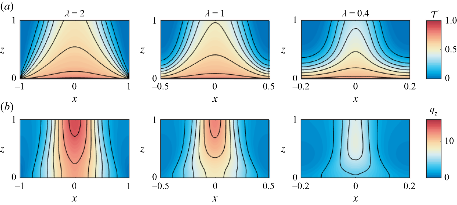
The physical origin of the stable, highly localised branch can be readily understood as the wider region of the fissure remaining in the hot, fast flowing state, while the thinner region transitions to the cold, slow state as the pressure drop decreases. The flow in the wider region is cognate with the fast branch of the planar solution, and the flow in the narrower region is cognate with the slow branch of the planar solution. Thus, the occurrence of geometrical focussing is more closely associated with the fold bifurcation and planar instability exhibited by the uniform-width system than it is with the thermoviscous fingering instability. The dependence on amplitude and wavelength can also be easily explained. Naturally, a larger amplitude results in a greater difference in flow rate and hence heat advection through the different regions of the fissure. However, if the wavelength is small, then the hot and cold regions can exchange heat more easily, resulting in a more uniform temperature and a reduction in the geometric effect. Note that this exchange of heat does not occur diffusively, since the reduced heat equation includes no diffusion in the plane of the fissure (see (2.9)); rather, it occurs through advection due to along-fissure pressure gradients. These pressure gradients are stronger when the length scale between the regions of the fissure are smaller, and thus the solutions become more uniform for smaller
 $\lambda$
(e.g. compare solutions for
$\lambda$
(e.g. compare solutions for
 $\lambda = 2$
and
$\lambda = 2$
and
 $\lambda = 0.4$
in figure 6). Another way to understand the suppression of geometrical localisation at short geometrical wavelength is by reference to the fingering instability in the uniform geometry. Here, Wylie & Lister (Reference Wylie and Lister1995) and Morris (Reference Morris1996) showed that the preferred wavelength of the fingering instability is comparable to, or larger than, the thermal entry length, which scales with
$\lambda = 0.4$
in figure 6). Another way to understand the suppression of geometrical localisation at short geometrical wavelength is by reference to the fingering instability in the uniform geometry. Here, Wylie & Lister (Reference Wylie and Lister1995) and Morris (Reference Morris1996) showed that the preferred wavelength of the fingering instability is comparable to, or larger than, the thermal entry length, which scales with
 $Q$
. The geometrical localisation occurs via the above mentioned mechanism at values of
$Q$
. The geometrical localisation occurs via the above mentioned mechanism at values of
 $\Pi$
near the location of the fold bifurcations associated with multiplicity of steady states in the planar problem (see figure 4), and hence at solutions which have fluxes of the order
$\Pi$
near the location of the fold bifurcations associated with multiplicity of steady states in the planar problem (see figure 4), and hence at solutions which have fluxes of the order
 $1\lesssim Q\lesssim 10$
. Therefore, by analogy with the result for the uniform geometry, for geometrical wavelengths significantly smaller than these
$1\lesssim Q\lesssim 10$
. Therefore, by analogy with the result for the uniform geometry, for geometrical wavelengths significantly smaller than these
 $O(1)$
thermal entry lengths, the localisation into features on the length scale of the topography is suppressed.
$O(1)$
thermal entry lengths, the localisation into features on the length scale of the topography is suppressed.
3.3. Long-wavelength regime
In the regime of long wavelength,
 $\lambda \gg 1$
, the different regions of the fissure are unable to ‘communicate’ with one another and a leading order analysis can be undertaken in which
$\lambda \gg 1$
, the different regions of the fissure are unable to ‘communicate’ with one another and a leading order analysis can be undertaken in which
 $x$
-derivatives vanish, and every vertical slice of the fissure can be considered as a planar problem of a different thickness. This regime is an interesting end member and could represent the variation of fissure width on the length scale set by the full length of the fissure – typically fissures are widest at their centres and get increasingly thin towards their ends. When the wavelength of the perturbation to the width is long, we can rescale the
$x$
-derivatives vanish, and every vertical slice of the fissure can be considered as a planar problem of a different thickness. This regime is an interesting end member and could represent the variation of fissure width on the length scale set by the full length of the fissure – typically fissures are widest at their centres and get increasingly thin towards their ends. When the wavelength of the perturbation to the width is long, we can rescale the
 $x$
-coordinate by
$x$
-coordinate by
 $\lambda$
and consider the variables to be asymptotic series in
$\lambda$
and consider the variables to be asymptotic series in
 $1/\lambda \ll 1$
. Taking only the leading order of the governing equations, we obtain
$1/\lambda \ll 1$
. Taking only the leading order of the governing equations, we obtain
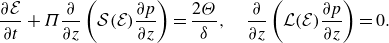 \begin{equation} \frac {\partial {\mathcal{E}}}{\partial t}+\Pi \frac {\partial }{\partial z}\left ( \mathcal{S}({\mathcal{E}})\frac {\partial p}{\partial z}\right )=\frac {2\Theta }{\delta }, \quad \frac {\partial }{\partial z}\left ({\mathcal{L}}({\mathcal{E}})\frac {\partial p}{\partial z}\right )=0. \end{equation}
Namely, the equations for the planar problem, with
 $x$
entering only as a parameter via the width,
$x$
entering only as a parameter via the width,
 $h(x)$
. These equations and the resulting steady-state flux,
$h(x)$
. These equations and the resulting steady-state flux,
 $Q$
, can then be rescaled to the case with
$Q$
, can then be rescaled to the case with
 $h=1$
, by writing
$h=1$
, by writing
 \begin{equation} {\mathcal{E}}=h\tilde {{\mathcal{E}}}, \,\,\delta =h\tilde {\delta }, \,\,{\mathcal{S}}=h^3\tilde {\mathcal{S}}, \,\,{\mathcal{L}}=h^3\tilde {\mathcal{L}}, \,\,\Pi =\tilde {\Pi }/h^4, \,t=h^2\tilde {t}, \text{ and } Q=\tilde {Q}/h. \end{equation}
Thus, given the uniform steady-state solution curve
 $(\Pi _0, Q_0)$
, we can find a steady-state solution curve for the position
$(\Pi _0, Q_0)$
, we can find a steady-state solution curve for the position
 $x$
in the non-uniform fissure, as
$x$
in the non-uniform fissure, as
 $(\Pi _0/h^4, Q_0/h)$
. In particular, at the widest region, we have
$(\Pi _0/h^4, Q_0/h)$
. In particular, at the widest region, we have
 $h=1+A$
and at the thinnest region, we have
$h=1+A$
and at the thinnest region, we have
 $h=1-A$
. Figure 7(a) shows the result of this rescaling for
$h=1-A$
. Figure 7(a) shows the result of this rescaling for
 $A=0.02$
: the wider geometry (dashed) exhibits a higher flux and consequently transitions from the fast branch to the slow branch via a pair of fold bifurcations at a lower pressure drop; conversely, the narrower geometry (dotted) exhibits a lower flux and transitions between the branches at a higher pressure drop. If we then consider the average of the fluxes at each pressure drop, we obtain a new curve shown by the solid curve. The curve in figure 7(b) shows the prediction for the ratio of fluxes,
$A=0.02$
: the wider geometry (dashed) exhibits a higher flux and consequently transitions from the fast branch to the slow branch via a pair of fold bifurcations at a lower pressure drop; conversely, the narrower geometry (dotted) exhibits a lower flux and transitions between the branches at a higher pressure drop. If we then consider the average of the fluxes at each pressure drop, we obtain a new curve shown by the solid curve. The curve in figure 7(b) shows the prediction for the ratio of fluxes,
 $Q_r\equiv Q_+/Q_-$
, in the wider and thinner regions of the fissure, from this long-wavelength analysis. From these two panels, we observe that the solution curve exhibits the key features of the non-uniform geometries at larger wavelengths, namely a stable middle branch with significant flux localisation (large
$Q_r\equiv Q_+/Q_-$
, in the wider and thinner regions of the fissure, from this long-wavelength analysis. From these two panels, we observe that the solution curve exhibits the key features of the non-uniform geometries at larger wavelengths, namely a stable middle branch with significant flux localisation (large
 $Q_r$
), connected to the fast and slow branches by two pairs of fold bifurcations. Also shown as points in each panel are the results of numerical solutions for
$Q_r$
), connected to the fast and slow branches by two pairs of fold bifurcations. Also shown as points in each panel are the results of numerical solutions for
 $A=0.02$
and
$A=0.02$
and
 $\lambda =20$
. These were obtained by natural continuation in decreasing
$\lambda =20$
. These were obtained by natural continuation in decreasing
 $\Pi$
, so the whole solution curve is not obtained; however, the branches that are obtained match the predictions well, closely capturing the maximum and minimum fluxes,
$\Pi$
, so the whole solution curve is not obtained; however, the branches that are obtained match the predictions well, closely capturing the maximum and minimum fluxes,
 $Q_+$
and
$Q_+$
and
 $Q_-$
, and their ratio,
$Q_-$
, and their ratio,
 $Q_r$
, and showing roughly the same critical pressure drops where the solutions change from one branch to another.
$Q_r$
, and showing roughly the same critical pressure drops where the solutions change from one branch to another.
(a) Steady-state solution curve (as in figure 3) for the uniform geometry,
 $h=1$
, re-scaled to the width of the widest,
$h=1$
, re-scaled to the width of the widest,
 $h=1+A$
(black dashed), and thinnest,
$h=1+A$
(black dashed), and thinnest,
 $h=1-A$
(black dotted), regions of the non-uniform geometry with
$h=1-A$
(black dotted), regions of the non-uniform geometry with
 $A=0.02$
and
$A=0.02$
and
 $\lambda \to \infty$
according to (3.2). These represent the maximum,
$\lambda \to \infty$
according to (3.2). These represent the maximum,
 $Q_+$
, and minimum,
$Q_+$
, and minimum,
 $Q_-$
, surface fluxes in the non-uniform geometry. The black solid curve shows the average of the fluxes,
$Q_-$
, surface fluxes in the non-uniform geometry. The black solid curve shows the average of the fluxes,
 $(Q_++Q_-)/2$
. Points are shown from numerical solutions with
$(Q_++Q_-)/2$
. Points are shown from numerical solutions with
 $A=0.02$
and
$A=0.02$
and
 $\lambda =20$
, obtained by natural parameter continuation in decreasing
$\lambda =20$
, obtained by natural parameter continuation in decreasing
 $\Pi$
(
$\Pi$
(
 $Q_+$
, squares;
$Q_+$
, squares;
 $Q_-$
, crosses; average, circles). (b) Ratio of maximum and minimum flux,
$Q_-$
, crosses; average, circles). (b) Ratio of maximum and minimum flux,
 $Q_r=Q_+/Q_-$
, as a function of
$Q_r=Q_+/Q_-$
, as a function of
 $\Pi$
. The line is obtained from taking the ratio of the fluxes represented by the dashed and dotted lines in panel (a), and the circles are obtained from the numerical simulations, as in panel (a). (c) Average flux per unit length,
$\Pi$
. The line is obtained from taking the ratio of the fluxes represented by the dashed and dotted lines in panel (a), and the circles are obtained from the numerical simulations, as in panel (a). (c) Average flux per unit length,
 $Q$
, as a function of
$Q$
, as a function of
 $\Pi$
. The lines are obtained by the long wavelength approximation (3.4). The different curves correspond to continuation in
$\Pi$
. The lines are obtained by the long wavelength approximation (3.4). The different curves correspond to continuation in
 $\Pi$
in either the decreasing (solid) or increasing (dashed) directions. Also shown as circles are the numerical results as in panels (a) and (b). (d) Colour plot of scaled surface flux ratio,
$\Pi$
in either the decreasing (solid) or increasing (dashed) directions. Also shown as circles are the numerical results as in panels (a) and (b). (d) Colour plot of scaled surface flux ratio,
 $\tilde {Q}_r$
(defined by (2.29)), as a function of
$\tilde {Q}_r$
(defined by (2.29)), as a function of
 $\Pi$
and
$\Pi$
and
 $A$
for numerical solutions with
$A$
for numerical solutions with
 $\lambda =20$
. The solid red lines show the boundaries predicted by the long-wavelength analysis (
$\lambda =20$
. The solid red lines show the boundaries predicted by the long-wavelength analysis (
 $\Pi =241/(1+A)^4$
and
$\Pi =241/(1+A)^4$
and
 $\Pi =241/(1-A)^4$
), and the red dotted line shows the predicted lower boundary offset by a pressure drop of
$\Pi =241/(1-A)^4$
), and the red dotted line shows the predicted lower boundary offset by a pressure drop of
 $5$
. Note the logarithmic colour scale. See table 2 for other parameters used in these solutions.
$5$
. Note the logarithmic colour scale. See table 2 for other parameters used in these solutions.
We note that the use of the average of the largest and smallest fluxes,
 $(Q_++Q_-)/2$
, in figure 7(a) is not the same as the average flux per unit length,
$(Q_++Q_-)/2$
, in figure 7(a) is not the same as the average flux per unit length,
 $Q$
, used previously, but was chosen here for illustrative purposes. To obtain the prediction for
$Q$
, used previously, but was chosen here for illustrative purposes. To obtain the prediction for
 $Q$
, we must account for the continuous variation of the width,
$Q$
, we must account for the continuous variation of the width,
 $h$
. Suppose we have the flux as a function of the pressure drop,
$h$
. Suppose we have the flux as a function of the pressure drop,
 $Q_0(\Pi _0)$
, from the uniform geometry results (the choices made in defining such a function are discussed later). To obtain a long wavelength prediction for the average flux per unit length of the non-uniform geometry, we can then calculate
$Q_0(\Pi _0)$
, from the uniform geometry results (the choices made in defining such a function are discussed later). To obtain a long wavelength prediction for the average flux per unit length of the non-uniform geometry, we can then calculate
 \begin{equation} Q(\Pi ) \approx \frac {1}{L_x}\int _0^{L_x} \frac {Q_0(h(x)^4\Pi )}{h(x)}\, \textrm {d}x, \end{equation}
which, for the sinusoidal width,
 $h=1+A\cos (2\pi x/\lambda )$
, is independent of wavelength
$h=1+A\cos (2\pi x/\lambda )$
, is independent of wavelength
 \begin{equation} Q(\Pi ) \approx \frac {2}{\lambda }\int _0^{\lambda /2} \frac {Q_0(h^4\Pi )}{h}\, \textrm {d}x=\frac {1}{\pi }\int _{1-A}^{1+A} \frac {Q_0(h^4\Pi )}{h\sqrt {A^2-(1-h)^2}} \,\textrm {d}h . \end{equation}
We note that the solution curve
 $(\Pi _0,Q_0)$
does not immediately provide a well-defined function
$(\Pi _0,Q_0)$
does not immediately provide a well-defined function
 $Q_0(\Pi _0)$
, due to the multiplicity of steady states. There is, however, a natural choice by which to define two such functions, corresponding to natural parameter continuation in either decreasing or increasing
$Q_0(\Pi _0)$
, due to the multiplicity of steady states. There is, however, a natural choice by which to define two such functions, corresponding to natural parameter continuation in either decreasing or increasing
 $\Pi$
. For the former, wherever
$\Pi$
. For the former, wherever
 $Q_0(\Pi _0)$
is multivalued, we choose to take
$Q_0(\Pi _0)$
is multivalued, we choose to take
 $Q_0$
from the fast, hot branch, while in the latter, we instead evaluate the flux from the slow, cold branch. The resulting predictions for the average flux,
$Q_0$
from the fast, hot branch, while in the latter, we instead evaluate the flux from the slow, cold branch. The resulting predictions for the average flux,
 $Q$
, for the sinusoidal geometry with
$Q$
, for the sinusoidal geometry with
 $A=0.02$
are shown in figure 7(c). Here, the solid line is for the natural continuation in decreasing
$A=0.02$
are shown in figure 7(c). Here, the solid line is for the natural continuation in decreasing
 $\Pi$
and is compared against the fluxes obtained from the numerical solutions with
$\Pi$
and is compared against the fluxes obtained from the numerical solutions with
 $\lambda =20$
(circles, also obtained by continuation in decreasing
$\lambda =20$
(circles, also obtained by continuation in decreasing
 $\Pi$
). These show good agreement. The dashed line, for comparison, shows the prediction for natural continuation in increasing
$\Pi$
). These show good agreement. The dashed line, for comparison, shows the prediction for natural continuation in increasing
 $\Pi$
, giving a lower flux where the two differ.
$\Pi$
, giving a lower flux where the two differ.
For the current parameters and the uniform geometry,
 $h=1$
, the fold bifurcation on the fast branch occurs at
$h=1$
, the fold bifurcation on the fast branch occurs at
 $\Pi \approx 241$
at which the flux drops from
$\Pi \approx 241$
at which the flux drops from
 $Q\approx 6.6$
to
$Q\approx 6.6$
to
 $Q\approx 1$
(when continuing naturally in decreasing
$Q\approx 1$
(when continuing naturally in decreasing
 $\Pi$
). Thus, for the long-wavelength approximation, we anticipate the first fold bifurcation to occur at
$\Pi$
). Thus, for the long-wavelength approximation, we anticipate the first fold bifurcation to occur at
 $\Pi =241/(1-A)^4$
. At this bifurcation, the thinner region exhibits a reduction in flux by a factor of
$\Pi =241/(1-A)^4$
. At this bifurcation, the thinner region exhibits a reduction in flux by a factor of
 $6.6/(1-A)$
, while the wider region maintains the same flux. Thus, the surface flux ratio increases by a factor of
$6.6/(1-A)$
, while the wider region maintains the same flux. Thus, the surface flux ratio increases by a factor of
 $6.6/(1-A)$
when the solution drops onto the focussed branch at this point. The second fold bifurcation is predicted to occur at
$6.6/(1-A)$
when the solution drops onto the focussed branch at this point. The second fold bifurcation is predicted to occur at
 $\Pi =241/(1+A)^4$
, where the surface flux ratio decreases by a factor of
$\Pi =241/(1+A)^4$
, where the surface flux ratio decreases by a factor of
 $6.6/(1+A)$
. Thus, as the amplitude,
$6.6/(1+A)$
. Thus, as the amplitude,
 $A$
, decreases towards zero, the stable focussed branch shortens but persists, ultimately shrinking to the point
$A$
, decreases towards zero, the stable focussed branch shortens but persists, ultimately shrinking to the point
 $\Pi =241$
, with
$\Pi =241$
, with
 $Q_+=6.6$
and
$Q_+=6.6$
and
 $Q_-=1$
, as
$Q_-=1$
, as
 $A\to 0$
. The prediction for the critical values of
$A\to 0$
. The prediction for the critical values of
 $\Pi$
which bound the focussed branch is compared with numerical solutions for
$\Pi$
which bound the focussed branch is compared with numerical solutions for
 $\lambda =20$
in figure 7(c) showing good agreement for the upper boundary,
$\lambda =20$
in figure 7(c) showing good agreement for the upper boundary,
 $\Pi =241/(1-A)^4$
, but weaker agreement for the lower boundary where the long-wavelength analysis under-predicts the critical pressure drops observed in the numerical solutions by roughly
$\Pi =241/(1-A)^4$
, but weaker agreement for the lower boundary where the long-wavelength analysis under-predicts the critical pressure drops observed in the numerical solutions by roughly
 $5$
at all amplitudes (this is also noticeable in the other panels of figure 7 for the specific choice of
$5$
at all amplitudes (this is also noticeable in the other panels of figure 7 for the specific choice of
 $A=0.02$
). It is unclear what causes this discrepancy. However, since the thinner region lies on the slow branch of the solution curve, it becomes unstable to the thermoviscous fingering instability, resulting in finger structures within the cool, slow region of the fissure. The wavelength of these fingers decreases with decreasing pressure drop,
$A=0.02$
). It is unclear what causes this discrepancy. However, since the thinner region lies on the slow branch of the solution curve, it becomes unstable to the thermoviscous fingering instability, resulting in finger structures within the cool, slow region of the fissure. The wavelength of these fingers decreases with decreasing pressure drop,
 $\Pi$
, and so it is possible that the assumption of large length scale in the
$\Pi$
, and so it is possible that the assumption of large length scale in the
 $x$
-direction becomes invalid at the boundary between the hot and cold regions as the critical pressure drop is approached. In general, if gradients are greater in the
$x$
-direction becomes invalid at the boundary between the hot and cold regions as the critical pressure drop is approached. In general, if gradients are greater in the
 $x$
-direction than implied by the rough scaling,
$x$
-direction than implied by the rough scaling,
 $1/\lambda \ll 1$
, this will promote heat fluxes between the regions, resulting in a transition to the uniformly slow branch at larger
$1/\lambda \ll 1$
, this will promote heat fluxes between the regions, resulting in a transition to the uniformly slow branch at larger
 $\Pi$
. Nonetheless, the predictions of the long-wavelength analysis give a decent agreement to the numerical solutions, particularly for the critical pressure drop resulting in the onset of localisation, which is perhaps of greatest concern for the volcanological application.
$\Pi$
. Nonetheless, the predictions of the long-wavelength analysis give a decent agreement to the numerical solutions, particularly for the critical pressure drop resulting in the onset of localisation, which is perhaps of greatest concern for the volcanological application.
(a,b) Scaled surface flux ratios,
 $\tilde {Q}_r$
, as a function of the dimensionless pressure drop,
$\tilde {Q}_r$
, as a function of the dimensionless pressure drop,
 $\Pi$
, for steady and periodic solutions with
$\Pi$
, for steady and periodic solutions with
 $A=0.02$
and
$A=0.02$
and
 $\lambda =2$
over two ranges of
$\lambda =2$
over two ranges of
 $\Pi$
corresponding to the absence of stable steady states in figure 5(b). For periodic solutions, the maximum and minimum values of
$\Pi$
corresponding to the absence of stable steady states in figure 5(b). For periodic solutions, the maximum and minimum values of
 $\tilde {Q}_r$
are plotted as solid lines, and the average over the period is plotted as a dotted line. Markers indicate the bifurcations at which the steady branches lose stability, with triangles corresponding to infinite period bifurcations and the dot indicating a supercritical Hopf bifurcation. (c,d) Period of the solutions as a function of
$\tilde {Q}_r$
are plotted as solid lines, and the average over the period is plotted as a dotted line. Markers indicate the bifurcations at which the steady branches lose stability, with triangles corresponding to infinite period bifurcations and the dot indicating a supercritical Hopf bifurcation. (c,d) Period of the solutions as a function of
 $\Pi$
, with the two panels corresponding to the branches shown in panel (a,b). Red dashed lines indicate the ends of the stable steady-state solution branches at either side. See table 2 for other parameters used in these solutions.
$\Pi$
, with the two panels corresponding to the branches shown in panel (a,b). Red dashed lines indicate the ends of the stable steady-state solution branches at either side. See table 2 for other parameters used in these solutions.
3.4. Periodic solutions
Here, we detail the origin and the bifurcation structure of the periodic solutions evidenced by the absence of steady states at points marked in red in figure 5(b). We take two examples of branches of periodic solutions along the solution curve for
 $A=0.02$
and
$A=0.02$
and
 $\lambda =2$
, tracking the solutions as
$\lambda =2$
, tracking the solutions as
 $\Pi$
is varied. For these solutions, we took
$\Pi$
is varied. For these solutions, we took
 $L_x=1$
, i.e. the smallest domain that captures the
$L_x=1$
, i.e. the smallest domain that captures the
 $\lambda =2$
wavelength, given the symmetry boundary conditions at either end. The scaled surface flux ratio,
$\lambda =2$
wavelength, given the symmetry boundary conditions at either end. The scaled surface flux ratio,
 $\tilde {Q}_r$
, and the period are plotted as functions of
$\tilde {Q}_r$
, and the period are plotted as functions of
 $\Pi$
in figure 8, showing that one periodic solution branch persists over the range
$\Pi$
in figure 8, showing that one periodic solution branch persists over the range
 $202.6\lesssim \Pi \lesssim 216$
and two different periodic branches occur over the range
$202.6\lesssim \Pi \lesssim 216$
and two different periodic branches occur over the range
 $229.4\lesssim \Pi \lesssim 233.8$
. At
$229.4\lesssim \Pi \lesssim 233.8$
. At
 $\Pi \approx 233.8$
, on the steady solution branch, a pair of complex eigenvalues of the stability problem cross the imaginary axis, indicating a Hopf bifurcation. The amplitude of the stable periodic solutions obtained near
$\Pi \approx 233.8$
, on the steady solution branch, a pair of complex eigenvalues of the stability problem cross the imaginary axis, indicating a Hopf bifurcation. The amplitude of the stable periodic solutions obtained near
 $\Pi =233.8$
grows from zero, and their period starts at that of the unstable periodic mode at the bifurcation,
$\Pi =233.8$
grows from zero, and their period starts at that of the unstable periodic mode at the bifurcation,
 $2\pi/\textrm{Im} (\sigma )\approx 38$
. Thus, the bifurcation to the periodic solution is a supercritical Hopf bifurcation (e.g. see Strogatz Reference Strogatz2015b
). The periodic solution branch arising at the Hopf bifurcation is short-lived, becoming unstable to a fold bifurcation at
$2\pi/\textrm{Im} (\sigma )\approx 38$
. Thus, the bifurcation to the periodic solution is a supercritical Hopf bifurcation (e.g. see Strogatz Reference Strogatz2015b
). The periodic solution branch arising at the Hopf bifurcation is short-lived, becoming unstable to a fold bifurcation at
 $\Pi \approx 233.45$
, resulting in the system transitioning to a new stable periodic solution branch, with a longer period and larger amplitude. At the other end of this periodic solution branch, the periodic solution is destroyed in an infinite period bifurcation at
$\Pi \approx 233.45$
, resulting in the system transitioning to a new stable periodic solution branch, with a longer period and larger amplitude. At the other end of this periodic solution branch, the periodic solution is destroyed in an infinite period bifurcation at
 $\Pi \approx 229.4$
, where a saddle-node point appears on the periodic orbit and the system follows the new stable steady-state solution branch at lower
$\Pi \approx 229.4$
, where a saddle-node point appears on the periodic orbit and the system follows the new stable steady-state solution branch at lower
 $\Pi$
. The period-averaged scaled surface flux ratio,
$\Pi$
. The period-averaged scaled surface flux ratio,
 $\tilde {Q}_r$
, is naturally continuous at this bifurcation, since the periodic solution spends an increasing proportion of its (diverging) period close to the state that becomes the stable steady solution after the bifurcation. For the second periodic solution branch, shown in figure 8(a,c), the bifurcation structure is slightly different, with the transition between the steady-state and periodic solution branch resulting from an infinite period bifurcation at both ends.
$\tilde {Q}_r$
, is naturally continuous at this bifurcation, since the periodic solution spends an increasing proportion of its (diverging) period close to the state that becomes the stable steady solution after the bifurcation. For the second periodic solution branch, shown in figure 8(a,c), the bifurcation structure is slightly different, with the transition between the steady-state and periodic solution branch resulting from an infinite period bifurcation at both ends.
Figure 9 shows the dimensionless average temperature,
 ${\mathcal{T}}(x,z)$
(see (2.13)), for a selection of solutions along the same solution branch (i.e. for the sinusoidal geometry with
${\mathcal{T}}(x,z)$
(see (2.13)), for a selection of solutions along the same solution branch (i.e. for the sinusoidal geometry with
 $A=0.02$
and
$A=0.02$
and
 $\lambda =2$
). Panels (a)–(c) show steady solutions at
$\lambda =2$
). Panels (a)–(c) show steady solutions at
 $\Pi =200$
,
$\Pi =200$
,
 $220$
and
$220$
and
 $234$
, representing solutions on the three steady-state branches separated by the periodic solution branches in figure 8. These indicate how the spatial structure of the fingered states changes after passing through the periodic solution branches. The other panels show three states obtained at particular times (with
$234$
, representing solutions on the three steady-state branches separated by the periodic solution branches in figure 8. These indicate how the spatial structure of the fingered states changes after passing through the periodic solution branches. The other panels show three states obtained at particular times (with
 $t=0$
chosen arbitrarily) during the periodic solutions at
$t=0$
chosen arbitrarily) during the periodic solutions at
 $\Pi =210$
(panels d–f) and
$\Pi =210$
(panels d–f) and
 $\Pi =232$
(panels g–i), indicating that these solutions exhibit oscillations between states that are similar in structure to stable steady solutions at larger and smaller values of
$\Pi =232$
(panels g–i), indicating that these solutions exhibit oscillations between states that are similar in structure to stable steady solutions at larger and smaller values of
 $\Pi$
. While the exact details of two fingered solutions might vary subtly, there are two main factors that govern the broad configuration of a solution. The first is the number of fingers in the domain or, equivalently, the average wavelength of the fingers. The second is the location of these fingers, which (given the symmetry boundary conditions) largely corresponds to a binary choice of whether
$\Pi$
. While the exact details of two fingered solutions might vary subtly, there are two main factors that govern the broad configuration of a solution. The first is the number of fingers in the domain or, equivalently, the average wavelength of the fingers. The second is the location of these fingers, which (given the symmetry boundary conditions) largely corresponds to a binary choice of whether
 $x=0$
corresponds to a (relatively) hot or cold region of the fissure. As for the uniform case (see figure 3
b), the preferred wavelength of fingers scales with the thermal entry length and, thus, the average wavelength increases as
$x=0$
corresponds to a (relatively) hot or cold region of the fissure. As for the uniform case (see figure 3
b), the preferred wavelength of fingers scales with the thermal entry length and, thus, the average wavelength increases as
 $\Pi$
increases. For example, at
$\Pi$
increases. For example, at
 $\Pi =200$
(figure 9
a), the solution exhibits five hot fingers per wavelength of the fissure geometry (half of this wavelength,
$\Pi =200$
(figure 9
a), the solution exhibits five hot fingers per wavelength of the fissure geometry (half of this wavelength,
 $\lambda =2$
, is shown in each panel), while at
$\lambda =2$
, is shown in each panel), while at
 $\Pi =220$
and
$\Pi =220$
and
 $\Pi =234$
(figure 9
b,c), there are four. In the non-uniform geometry, the preferred wavelength also depends on the local width of the channel, with longer wavelengths preferred in wider regions (since the thermal entry length also increases with channel width). This effect is visible in figure 9, where the wavelength of the fingering pattern generally gets shorter between the widest region of the channel, at
$\Pi =234$
(figure 9
b,c), there are four. In the non-uniform geometry, the preferred wavelength also depends on the local width of the channel, with longer wavelengths preferred in wider regions (since the thermal entry length also increases with channel width). This effect is visible in figure 9, where the wavelength of the fingering pattern generally gets shorter between the widest region of the channel, at
 $x=0$
, and the narrowest, at
$x=0$
, and the narrowest, at
 $x=1$
. The dependence on
$x=1$
. The dependence on
 $\Pi$
of the choice between a hot or cold region at
$\Pi$
of the choice between a hot or cold region at
 $x=0$
is less clear. Naively, one might anticipate that the most stable configuration would be one in which the widest point of the channel is hot and/or the narrowest point is cold. However, given the continuous variation of fissure width, the situation turns out to be more subtle than this. For example, at
$x=0$
is less clear. Naively, one might anticipate that the most stable configuration would be one in which the widest point of the channel is hot and/or the narrowest point is cold. However, given the continuous variation of fissure width, the situation turns out to be more subtle than this. For example, at
 $\Pi =200$
, both choices result in stable steady states. Similarly, both configurations arise during the periodic solution at
$\Pi =200$
, both choices result in stable steady states. Similarly, both configurations arise during the periodic solution at
 $\Pi =210$
(see figure 9
e,f). In figure 9(a), we show the state with a cold region at
$\Pi =210$
(see figure 9
e,f). In figure 9(a), we show the state with a cold region at
 $x=0$
, which is the solution reached when continuing in
$x=0$
, which is the solution reached when continuing in
 $\Pi$
from the periodic solution branch at
$\Pi$
from the periodic solution branch at
 $202.6\lessapprox \Pi \lessapprox 216$
(i.e. it is a state similar to that shown in figure 9(f), and not panel (e), that becomes the saddle-node point in the infinite period bifurcation at
$202.6\lessapprox \Pi \lessapprox 216$
(i.e. it is a state similar to that shown in figure 9(f), and not panel (e), that becomes the saddle-node point in the infinite period bifurcation at
 $\Pi \approx 202.6$
). This is also the configuration which is the more stable of the two at
$\Pi \approx 202.6$
). This is also the configuration which is the more stable of the two at
 $\Pi =200$
(in the sense that the growth rate of its least stable mode is more negative). In general, the preferred configuration depends on
$\Pi =200$
(in the sense that the growth rate of its least stable mode is more negative). In general, the preferred configuration depends on
 $\Pi$
. For example, both the solutions at
$\Pi$
. For example, both the solutions at
 $\Pi =220$
and
$\Pi =220$
and
 $\Pi =234$
in figure 9(b,c) have an average wavelength of 0.5, but the solutions have opposite configurations. There are thus several (potentially) competing influences on the configuration of fingers in a flow-focussed state: the preferred wavelength of fingers in an average sense; the preferred wavelength of fingers locally, due to the local channel width; and the relative stability of the two choices of finger location. The periodic solution branches then arise where these influences are in conflict and no choice of configuration is stable, with the solution instead oscillating between multiple, weakly unstable states. During a periodic orbit, the evolution between these states happens in two main ways: a propagation of the fingers down the length of the fissure (e.g. panels e
,f and g,
i in figure 9); or the removal or addition of a finger at one or both ends of the domain (e.g. the evolution to and from panels d and h). As demonstrated in figure 8, the periodic solution branches can evidence a range of different behaviours, and we do not claim to have provided an exhaustive exploration of these states. We also note that no periodic solutions were observed for the uniform geometry. Two of the factors previously discussed (the spatially varying preferred wavelength, and the choice for the location of the hot and cold fingers) are absent without the presence of wider and narrower regions of the fissure, and so it is perhaps unsurprising that the uniform geometry does not exhibit oscillatory dynamics.
$\Pi =234$
in figure 9(b,c) have an average wavelength of 0.5, but the solutions have opposite configurations. There are thus several (potentially) competing influences on the configuration of fingers in a flow-focussed state: the preferred wavelength of fingers in an average sense; the preferred wavelength of fingers locally, due to the local channel width; and the relative stability of the two choices of finger location. The periodic solution branches then arise where these influences are in conflict and no choice of configuration is stable, with the solution instead oscillating between multiple, weakly unstable states. During a periodic orbit, the evolution between these states happens in two main ways: a propagation of the fingers down the length of the fissure (e.g. panels e
,f and g,
i in figure 9); or the removal or addition of a finger at one or both ends of the domain (e.g. the evolution to and from panels d and h). As demonstrated in figure 8, the periodic solution branches can evidence a range of different behaviours, and we do not claim to have provided an exhaustive exploration of these states. We also note that no periodic solutions were observed for the uniform geometry. Two of the factors previously discussed (the spatially varying preferred wavelength, and the choice for the location of the hot and cold fingers) are absent without the presence of wider and narrower regions of the fissure, and so it is perhaps unsurprising that the uniform geometry does not exhibit oscillatory dynamics.
Colour plots and contours of average temperature,
 ${\mathcal{T}}$
, for several solutions in the sinusoidal geometry with
${\mathcal{T}}$
, for several solutions in the sinusoidal geometry with
 $A=0.02$
and
$A=0.02$
and
 $\lambda =2$
. (a–c) Steady solutions at (a)
$\lambda =2$
. (a–c) Steady solutions at (a)
 $\Pi =200$
, (b)
$\Pi =200$
, (b)
 $\Pi =220$
and (c)
$\Pi =220$
and (c)
 $\Pi =234$
. Panels (d)–(f) and (g)–(i) show snapshots at several times in the periodic solutions at
$\Pi =234$
. Panels (d)–(f) and (g)–(i) show snapshots at several times in the periodic solutions at
 $\Pi =210$
(period
$\Pi =210$
(period
 $\approx 182$
) and
$\approx 182$
) and
 $\Pi =232$
(period
$\Pi =232$
(period
 $\approx 115$
), as indicated in the titles, and
$\approx 115$
), as indicated in the titles, and
 $t=0$
chosen without loss of generality. Contours are plotted from
$t=0$
chosen without loss of generality. Contours are plotted from
 ${\mathcal{T}}=0.1$
nearest the top of each panel, increasing in increments of
${\mathcal{T}}=0.1$
nearest the top of each panel, increasing in increments of
 ${\mathcal{T}}=0.1$
. The axes are the same in all panels, and are omitted from all but panel (a) to avoid crowding. See table 2 for other parameters used in these solutions.
${\mathcal{T}}=0.1$
. The axes are the same in all panels, and are omitted from all but panel (a) to avoid crowding. See table 2 for other parameters used in these solutions.
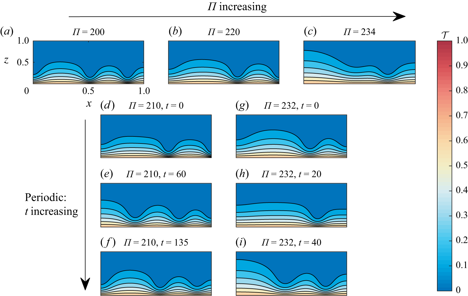
4. Discussion and implications
The results in § 3 indicate that geometric localisation in a dyke with sinusoidally varying width tends to overprint localisation via the thermoviscous fingering instability observed in planar dykes. It also leads to a greater degree of localisation under similar conditions: the magnitude of the surface flux ratio on the focussed branch takes substantially larger values (in the range
 $2{-}16$
for the results shown in figure 4) than those obtained for the steady state that arises through viscous fingering (see figure 3). Furthermore, the localisation occurs at higher pressure drops, before the entire system lies on the cold, slow branch. A 5 % non-uniformity,
$2{-}16$
for the results shown in figure 4) than those obtained for the steady state that arises through viscous fingering (see figure 3). Furthermore, the localisation occurs at higher pressure drops, before the entire system lies on the cold, slow branch. A 5 % non-uniformity,
 $A=0.05$
, is fairly modest compared with the variations seen in volcanic fissures (Parcheta et al. Reference Parcheta, Fagents, Swanson, Houghton and Ericksen2015), and figures 4 and 5 indicate that above this amplitude, there are large regions of the parameter space where there is significant localisation through geometric effects, particularly at large wavelengths. While many of the irregularities observed in natural systems have relatively short wavelengths (Parcheta et al. Reference Parcheta, Fagents, Swanson, Houghton and Ericksen2015), at the very least, fissures are typically wider at their centre and taper towards their ends (Daniels et al. Reference Daniels, Kavanagh, Menand and Sparks2012). The model we present does not extend to a fissure which is completely closed at its ends, but the full length of the fissure does set a large wavelength variation in fissure width. It therefore seems very plausible that the localisation of these natural systems is dominated by the non-uniformity of the geometry, rather than the spontaneous localisation driven by viscous fingering.
$A=0.05$
, is fairly modest compared with the variations seen in volcanic fissures (Parcheta et al. Reference Parcheta, Fagents, Swanson, Houghton and Ericksen2015), and figures 4 and 5 indicate that above this amplitude, there are large regions of the parameter space where there is significant localisation through geometric effects, particularly at large wavelengths. While many of the irregularities observed in natural systems have relatively short wavelengths (Parcheta et al. Reference Parcheta, Fagents, Swanson, Houghton and Ericksen2015), at the very least, fissures are typically wider at their centre and taper towards their ends (Daniels et al. Reference Daniels, Kavanagh, Menand and Sparks2012). The model we present does not extend to a fissure which is completely closed at its ends, but the full length of the fissure does set a large wavelength variation in fissure width. It therefore seems very plausible that the localisation of these natural systems is dominated by the non-uniformity of the geometry, rather than the spontaneous localisation driven by viscous fingering.
In practice, fissure geometries are not strictly sinusoidal, and natural variability is likely better represented by a random superposition of a range of wavelengths and amplitudes. While the nonlinearity of the system means that solutions cannot be formed simply by superposition of the solutions for the sinusoidal geometries, we nonetheless anticipate that the qualitative results regarding the occurrence of geometry-dominated flow focussing will carry across to such geometries. Rather than explore a wide range of different randomised geometries, here we give one example of the implications of the above mentioned conclusions for such a geometry. Fault and fracture geometries are often modelled by a power-law roughness,
 $P(\lambda )\propto \lambda ^{\alpha }$
, where
$P(\lambda )\propto \lambda ^{\alpha }$
, where
 $P(\lambda )$
is the power spectral density of the mode with wavelength
$P(\lambda )$
is the power spectral density of the mode with wavelength
 $\lambda$
and
$\lambda$
and
 $\alpha$
is a constant typically between 2 and 3 (Méheust & Schmittbuhl Reference Méheust and Schmittbuhl2000; Auradou et al. Reference Auradou, Drazer, Hulin and Koplik2005; Candela et al. Reference Candela, Renard, Klinger, Mair, Schmittbuhl and Brodsky2012; Brodsky et al. Reference Brodsky, Kirkpatrick and Candela2016). The geometry we consider has been generated with
$\alpha$
is a constant typically between 2 and 3 (Méheust & Schmittbuhl Reference Méheust and Schmittbuhl2000; Auradou et al. Reference Auradou, Drazer, Hulin and Koplik2005; Candela et al. Reference Candela, Renard, Klinger, Mair, Schmittbuhl and Brodsky2012; Brodsky et al. Reference Brodsky, Kirkpatrick and Candela2016). The geometry we consider has been generated with
 $L_x=1$
and
$L_x=1$
and
 $\alpha =2.2$
(the value reported by Brodsky et al. (Reference Brodsky, Kirkpatrick and Candela2016) for the geometry of fault surfaces), and we cut off the power-spectrum below a wavelength of
$\alpha =2.2$
(the value reported by Brodsky et al. (Reference Brodsky, Kirkpatrick and Candela2016) for the geometry of fault surfaces), and we cut off the power-spectrum below a wavelength of
 $\lambda =0.01$
, which would be poorly resolved at the resolution of the discrete grid. We further scale the values of
$\lambda =0.01$
, which would be poorly resolved at the resolution of the discrete grid. We further scale the values of
 $h$
such that
$h$
such that
 $0.95\leqslant h\leqslant 1.05$
, corresponding to
$0.95\leqslant h\leqslant 1.05$
, corresponding to
 $A=0.05$
in the case of the sinusoidal non-uniformity. The resulting randomised geometry is shown in the inset of figure 10(a). We then calculate steady and unsteady states of the system at different dimensionless pressure drops,
$A=0.05$
in the case of the sinusoidal non-uniformity. The resulting randomised geometry is shown in the inset of figure 10(a). We then calculate steady and unsteady states of the system at different dimensionless pressure drops,
 $\Pi$
, using the same numerical method as for the sinusoidal cases.
$\Pi$
, using the same numerical method as for the sinusoidal cases.
Figure 10(a) shows the surface flux,
 $q_z(x,z=1)$
, scaled by the total flux per unit length of the fissure,
$q_z(x,z=1)$
, scaled by the total flux per unit length of the fissure,
 $Q$
. As anticipated from the results for the sinusoidal case, when the pressure drop is sufficiently large or sufficiently small, the variation in the surface flux is fairly minor and is dictated primarily by the
$Q$
. As anticipated from the results for the sinusoidal case, when the pressure drop is sufficiently large or sufficiently small, the variation in the surface flux is fairly minor and is dictated primarily by the
 $h(x)^3$
factor for an isothermal fluid. In contrast, when the pressure drop takes intermediate values,
$h(x)^3$
factor for an isothermal fluid. In contrast, when the pressure drop takes intermediate values,
 $200\lesssim \Pi \lesssim 300$
, the system localises strongly at the positions of maximal width, due to the interaction between the geometry and the thermoviscosity. The region of
$200\lesssim \Pi \lesssim 300$
, the system localises strongly at the positions of maximal width, due to the interaction between the geometry and the thermoviscosity. The region of
 $\Pi$
and the magnitude of the flux ratio is consistent with the results for
$\Pi$
and the magnitude of the flux ratio is consistent with the results for
 $A=0.05$
in the sinusoidal case (see figures 4 and 5
c). Figure 10(b) shows the steady-state solution branch, with colours indicating the degree of flux localisation. Whereas the sinusoidal fissure geometries exhibit a single focussed branch, the solution curve for the randomised geometry suggests two successive stages of localisation. On decreasing the pressure drop, the system first transitions to a focussed state in which the left side of the fissure reduces in flux significantly, but three wider sections of the fissure remain at high flux states (see
$A=0.05$
in the sinusoidal case (see figures 4 and 5
c). Figure 10(b) shows the steady-state solution branch, with colours indicating the degree of flux localisation. Whereas the sinusoidal fissure geometries exhibit a single focussed branch, the solution curve for the randomised geometry suggests two successive stages of localisation. On decreasing the pressure drop, the system first transitions to a focussed state in which the left side of the fissure reduces in flux significantly, but three wider sections of the fissure remain at high flux states (see
 $\Pi =245$
in figure 10
a). A second transition occurs before
$\Pi =245$
in figure 10
a). A second transition occurs before
 $\Pi =235$
, where the thinner of these three sections enters the slow regime, leaving the fissure localised in the central region (see
$\Pi =235$
, where the thinner of these three sections enters the slow regime, leaving the fissure localised in the central region (see
 $\Pi =235$
in figure 10
a). Finally, the system transitions to the slow branch at
$\Pi =235$
in figure 10
a). Finally, the system transitions to the slow branch at
 $\Pi \approx 225$
, although the fissure remains fairly localised at the single widest point, where the flux gradually weakens as the pressure drop is decreased. The flux is largely uniform again by
$\Pi \approx 225$
, although the fissure remains fairly localised at the single widest point, where the flux gradually weakens as the pressure drop is decreased. The flux is largely uniform again by
 $\Pi =150$
. These transitions are further shown in figure 10(c), which plots the surface flux,
$\Pi =150$
. These transitions are further shown in figure 10(c), which plots the surface flux,
 $q_z$
, scaled by both the total flux per unit length of fissure,
$q_z$
, scaled by both the total flux per unit length of fissure,
 $Q$
, and the isothermal factor,
$Q$
, and the isothermal factor,
 $h^3$
. The localised branches are evidenced by regions of varying colour along slices of constant
$h^3$
. The localised branches are evidenced by regions of varying colour along slices of constant
 $\Pi$
.
$\Pi$
.
(a) Scaled vertical flux at the surface,
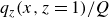 $q_z(x,z=1)/Q$
, as a function of position,
$q_z(x,z=1)/Q$
, as a function of position,
 $x$
, for the randomised geometry,
$x$
, for the randomised geometry,
 $h(x)$
, shown in the inset. The different coloured lines correspond to different dimensionless pressure drops,
$h(x)$
, shown in the inset. The different coloured lines correspond to different dimensionless pressure drops,
 $\Pi$
(see legend). The black dashed line shows the isothermal factor,
$\Pi$
(see legend). The black dashed line shows the isothermal factor,
 $h^3$
. (b) Steady-state solution curve for the randomised fissure geometry. Coloured points are stable solutions coloured according to the scaled surface flux ratio,
$h^3$
. (b) Steady-state solution curve for the randomised fissure geometry. Coloured points are stable solutions coloured according to the scaled surface flux ratio,
 $\tilde {Q}_r$
((2.30) with A = 0.05), and black circles indicate the solutions shown in panel (a), excluding
$\tilde {Q}_r$
((2.30) with A = 0.05), and black circles indicate the solutions shown in panel (a), excluding
 $\Pi =400$
which is off the scale. (c) Colour plot of surface flux,
$\Pi =400$
which is off the scale. (c) Colour plot of surface flux,
 $q_z(x,z=1)$
, scaled by
$q_z(x,z=1)$
, scaled by
 $h^3Q$
, as a function of position,
$h^3Q$
, as a function of position,
 $x$
, and pressure drop,
$x$
, and pressure drop,
 $\Pi$
. See table 2 for other parameters used in these solutions.
$\Pi$
. See table 2 for other parameters used in these solutions.
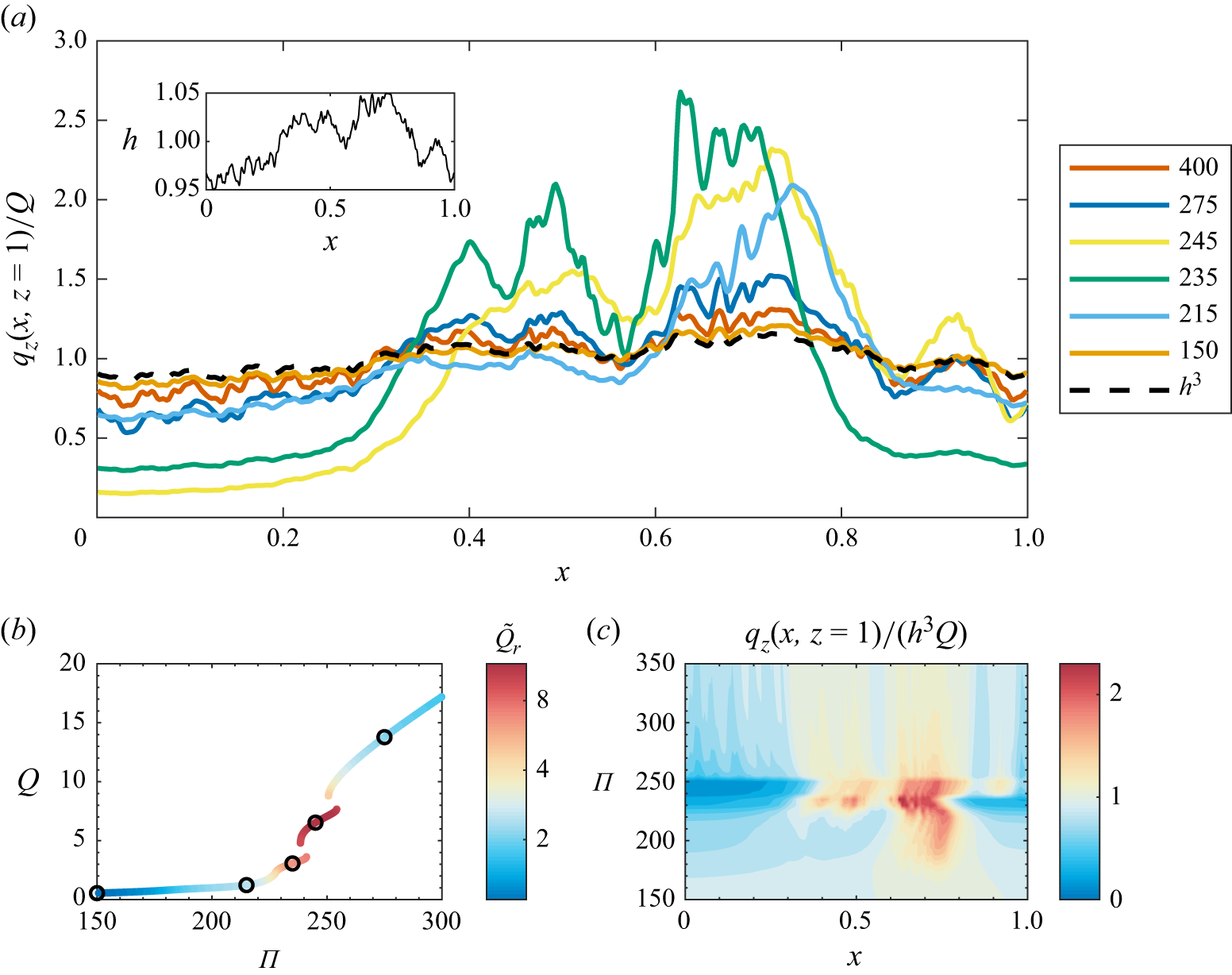
It is informative to consider the dimensional quantities for plausible volcanological parameters. As an illustrative example, we consider parameter values appropriate for a typical Hawaiian fissure eruption, as given in § 2. In this case, the flux scale is
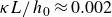 $\kappa L/h_0\approx 0.002$
m
$\kappa L/h_0\approx 0.002$
m
 $^{3}$
s–1 per metre length of the fissure. Thus, for the ranges of dimensionless flux per unit length,
$^{3}$
s–1 per metre length of the fissure. Thus, for the ranges of dimensionless flux per unit length,
 $Q$
, reported here, a kilometre of fissure would have a volume flux between 2 and 40 m
$Q$
, reported here, a kilometre of fissure would have a volume flux between 2 and 40 m
 $^{3}$
s–1, with the localisation occuring when the flux drops below approximately 20 m
$^{3}$
s–1, with the localisation occuring when the flux drops below approximately 20 m
 $^{3}$
s–1. This range of fluxes is consistent with estimates from fissure eruptions in Hawaii (Tilling et al. Reference Tilling, Christiansen, Duffield, Endo, Holcomb, Koyanagi, Peterson and Unger1987). It is also of interest to obtain some measure of the time scale on which the system evolves. Figure 11 shows one example of a time-dependent solution for the randomised fissure geometry shown in the inset of figure 10(a). In this case, the system was initiated with
$^{3}$
s–1. This range of fluxes is consistent with estimates from fissure eruptions in Hawaii (Tilling et al. Reference Tilling, Christiansen, Duffield, Endo, Holcomb, Koyanagi, Peterson and Unger1987). It is also of interest to obtain some measure of the time scale on which the system evolves. Figure 11 shows one example of a time-dependent solution for the randomised fissure geometry shown in the inset of figure 10(a). In this case, the system was initiated with
 $\Pi =245$
and with a temperature distribution close to the inlet temperature,
$\Pi =245$
and with a temperature distribution close to the inlet temperature,
 $T=1$
, throughout the fissure (specifically,
$T=1$
, throughout the fissure (specifically,
 ${\mathcal{E}}/h=0.01\implies {\mathcal{T}}=0.99$
everywhere). The system then evolves towards the steady state, which lies on one of the flow-focussed branches of the solution curve. As shown in figure 11, this relaxation to the new steady state occurs of the order of 2 dimensionless time units (becoming very close for
${\mathcal{E}}/h=0.01\implies {\mathcal{T}}=0.99$
everywhere). The system then evolves towards the steady state, which lies on one of the flow-focussed branches of the solution curve. As shown in figure 11, this relaxation to the new steady state occurs of the order of 2 dimensionless time units (becoming very close for
 $t\gtrapprox 4$
). This is also in line with the time scale implied by the decay rate of the least stable perturbation to the steady state, given by
$t\gtrapprox 4$
). This is also in line with the time scale implied by the decay rate of the least stable perturbation to the steady state, given by
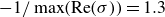 $-1/\max (\textrm{Re}(\sigma))=1.3$
. With the dimensional parameters for a typical Hawaiian fissure eruption given in § 2, the time scale,
$-1/\max (\textrm{Re}(\sigma))=1.3$
. With the dimensional parameters for a typical Hawaiian fissure eruption given in § 2, the time scale,
 $h_0^2/\kappa$
, is of the order of a day or two, and thus the adjustment shown in figure 11 would occur over the course of a few days. This is comparable to, although perhaps on the longer end of, the time scales for localisation observed in fissure eruptions (Richter et al. Reference Richter, Eaton, Murata, Ault and Krivoy1970; Thorarinsson et al. Reference Thorarinsson, Steinthórsson, Einarsson, Kristmannsdóttir and Oskarsson1973; Eibl et al. Reference Eibl, Bean, Jónsdóttir, Höskuldsson, Thordarson, Coppola, Witt and Walter2017). Additional physical effects, not incorporated into this model and discussed later, are likely to enhance localisation and thus shorten the time scale on which it occurs. Finally, we note that the typical dimensionless pressure drop,
$h_0^2/\kappa$
, is of the order of a day or two, and thus the adjustment shown in figure 11 would occur over the course of a few days. This is comparable to, although perhaps on the longer end of, the time scales for localisation observed in fissure eruptions (Richter et al. Reference Richter, Eaton, Murata, Ault and Krivoy1970; Thorarinsson et al. Reference Thorarinsson, Steinthórsson, Einarsson, Kristmannsdóttir and Oskarsson1973; Eibl et al. Reference Eibl, Bean, Jónsdóttir, Höskuldsson, Thordarson, Coppola, Witt and Walter2017). Additional physical effects, not incorporated into this model and discussed later, are likely to enhance localisation and thus shorten the time scale on which it occurs. Finally, we note that the typical dimensionless pressure drop,
 $\Pi =260$
, estimated for a dimensional pressure drop of
$\Pi =260$
, estimated for a dimensional pressure drop of
 $10^7$
Pa, is within the range where the geometrically flow-focussed solutions are typically found (
$10^7$
Pa, is within the range where the geometrically flow-focussed solutions are typically found (
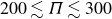 $200\lesssim \Pi \lesssim 300$
, see figures 4 and 10), and so it is plausible that this is a significant factor in the localisation of fissure eruptions.
$200\lesssim \Pi \lesssim 300$
, see figures 4 and 10), and so it is plausible that this is a significant factor in the localisation of fissure eruptions.
Evolution of surface flux,
 $q_z(x, z=1)$
, for the randomised fissure geometry when initiated at
$q_z(x, z=1)$
, for the randomised fissure geometry when initiated at
 $t=0$
from a uniformly hot state,
$t=0$
from a uniformly hot state,
 ${\mathcal{E}}/h=0.01$
, with
${\mathcal{E}}/h=0.01$
, with
 $\Pi =245$
. The steady-state solution for
$\Pi =245$
. The steady-state solution for
 $\Pi =245$
is indicated by the dashed black line, while the dotted line corresponds to the time scale implied by the slowest decay rate of linear perturbations to the steady state,
$\Pi =245$
is indicated by the dashed black line, while the dotted line corresponds to the time scale implied by the slowest decay rate of linear perturbations to the steady state,
 $t=-1/\max (\textrm{Re} (\sigma ))\approx 1.3$
. See table 2 for other parameters used in these solutions.
$t=-1/\max (\textrm{Re} (\sigma ))\approx 1.3$
. See table 2 for other parameters used in these solutions.
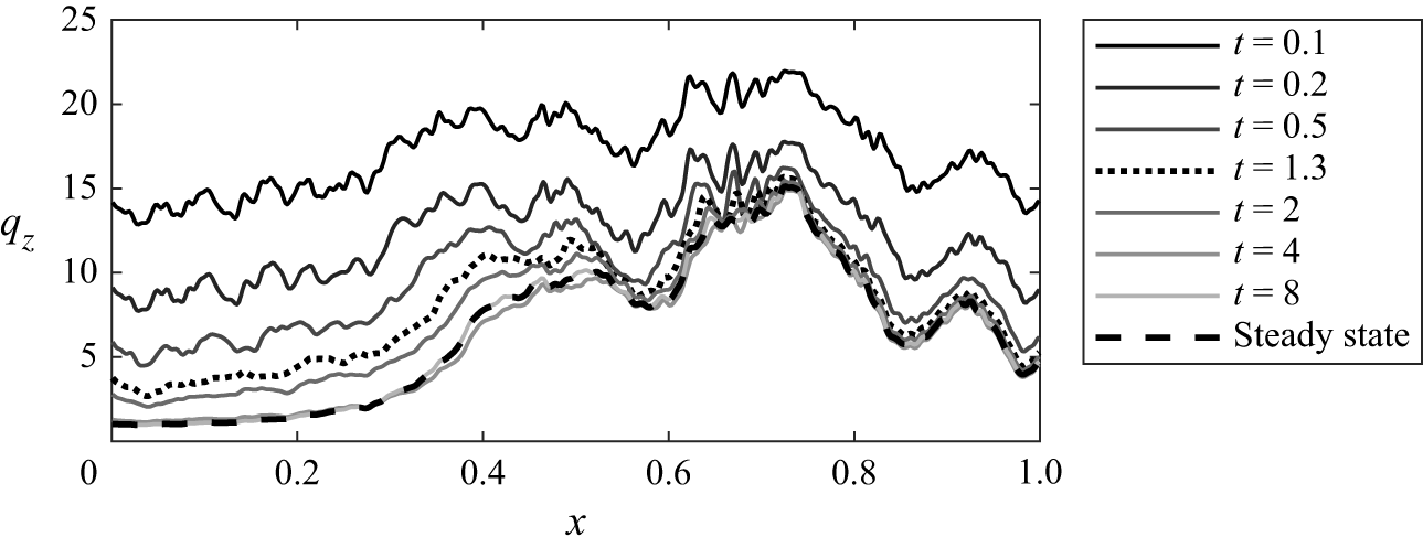
This work predominantly employed a width-averaged model, while retaining the essential structure of the cross-channel temperature profile, to efficiently capture the key qualitative behaviours of the non-uniform model. This averaging does introduce a quantitative departure from the true cross-channel temperature field, as discussed in Appendix B, and so comparisons to full three-dimensional numerical solutions, and analogue experiments, would be valuable. In addition to the full three-dimensional temperature field, there are a number of physical processes neglected in this model. A more complete treatment would include the thermodynamics at the fissure walls (including solidification), viscous heating and dissolution of volatiles from the magma in response to the vertically decreasing pressure. In particular, the latter would both introduce buoyant forcing (Pioli et al. Reference Pioli, Azzopardi, Bonadonna, Brunet and Kurokawa2017) and also couple to the rheology of the fluid (Mader, Llewellin & Mueller Reference Mader, Llewellin and Mueller2013), which could further enhance localisation. Solidification is likely to eventually transition the localised channel flow into a circular conduit flow, although the impact of solidification on the onset of localisation is believed to be minor due to the relatively slow time scale on which it occurs (Wylie et al. Reference Wylie, Helfrich, Dade, Lister and Salzig1999). Finally, here we considered only width variations that are aligned with the imposed pressure gradient. Such variations were considered most likely to support geometrically localised flow states; however, fissure geometries are typically more complex than this, and width variations in the flow direction are also common. It would therefore be valuable to explore the process of thermoviscous flow localisation in more general geometries.
5. Conclusion
We have studied the impact of a non-uniform fissure geometry on the localisation of a pressure-driven flow of fluid of a temperature-dependent viscosity, demonstrating that for topography aligned with the pressure gradient, relatively modest width variations and sufficiently long wavelengths, the most dramatic localisation occurs in response to the interaction between the thermoviscosity and the fissure geometry, rather than through spontaneous localisation through viscous fingering. This geometry-dominated localisation occurs due to the wider region of the fissure remaining on the hot, fast branch of the planar solution curve, while the thinner region transitions to the cold, slow branch. The resulting system is stable over a range of pressure drops and exhibits flux localisation roughly an order of magnitude larger than that of the steady flow-focussed states obtained through the viscous fingering instability in planar geometries. Furthermore, the geometry-dominated localisation typically occurs at larger pressure drops, since the fingering instability only occurs once the system lies on the slow branch of the solution curve. We have demonstrated that geometric localisation is effective for conditions appropriate to a typical Hawaiian fissure eruption and operates over time scales that are consistent with observations. It seems very plausible, therefore, that the localisation of volcanic fissure eruptions is controlled in large part by the pre-existing geometry of the fissure. This highlights the value in methods to accurately measure fissure geometry, both post-eruption (for example, using robotics, see Parcheta et al. Reference Parcheta, Pavlov, Wiltsie, Carpenter, Nash, Parness and Mitchell2016, or from measurements of eroded feeder dykes, see Daniels et al. Reference Daniels, Kavanagh, Menand and Sparks2012) and ideally also syneruptively, to help constrain the future localisation of the eruption and inform hazard prediction and mitigation.
Funding
This work was funded by the Engineering and Physical Sciences Research Council, UK, via the National Fellowship in Fluid Dynamics scheme [EP/X028011/1].
Declaration of interests
The authors report no conflict of interest.
Data availability statement
The data that support the findings of this study are available at https://doi.org/10.5281/zenodo.15660211 (Taylor-West & LLewellin Reference Taylor-West, LLewellin and Llewellin2025).
Appendix A. Numerical method
The governing equations in (2.22) are hyperbolic for
 ${\mathcal{E}}$
and elliptic for
${\mathcal{E}}$
and elliptic for
 $p$
. To avoid numerical instability of the nonlinear advection equation for
$p$
. To avoid numerical instability of the nonlinear advection equation for
 ${\mathcal{E}}$
, we discretise the system of equations via a first-order finite volume method, using upwinded fluxes in the
${\mathcal{E}}$
, we discretise the system of equations via a first-order finite volume method, using upwinded fluxes in the
 $z$
-direction. We define a grid with cell centres
$z$
-direction. We define a grid with cell centres
 $\{\boldsymbol{x}_{i,j}=(x_i,z_j): 1\leqslant i \leqslant N, 1\leqslant j \leqslant M\}$
, and cell size
$\{\boldsymbol{x}_{i,j}=(x_i,z_j): 1\leqslant i \leqslant N, 1\leqslant j \leqslant M\}$
, and cell size
 $\Delta x_i$
and
$\Delta x_i$
and
 $\Delta z_j$
in the
$\Delta z_j$
in the
 $x$
- and
$x$
- and
 $z$
-directions respectively (see figure 12
a). The cell-averaged values of
$z$
-directions respectively (see figure 12
a). The cell-averaged values of
 ${\mathcal{E}}$
and
${\mathcal{E}}$
and
 $p$
are written
$p$
are written
 $E_{i,j}$
and
$E_{i,j}$
and
 $P_{i,j}$
, respectively. Here,
$P_{i,j}$
, respectively. Here,
 $x_1=\Delta x_1/2$
,
$x_1=\Delta x_1/2$
,
 $x_N=L_x-\Delta x_N/2$
,
$x_N=L_x-\Delta x_N/2$
,
 $z_1=0$
and
$z_1=0$
and
 $z_M=1$
. In general, the size in the
$z_M=1$
. In general, the size in the
 $x$
-direction is taken uniform,
$x$
-direction is taken uniform,
 \begin{equation} \Delta x_i=\frac {L_x}{N_x}, \end{equation}
whereas the grid is concentrated near the inflow,
 $z=0$
, in the
$z=0$
, in the
 $z$
-direction to improve the resolution of the rapidly varying temperature here. In particular, we choose
$z$
-direction to improve the resolution of the rapidly varying temperature here. In particular, we choose
 \begin{equation} \Delta z_j = \frac {2j}{M^2-1}, \end{equation}
resulting in a quadratic spacing of the grid in this direction. We checked that solutions converge with
 $N$
and
$N$
and
 $M$
and chose a grid-size of
$M$
and chose a grid-size of
 $N=500$
and
$N=500$
and
 $M=200$
for the results reported here. For further verification of the numerical method, we employed our code with the averaging approach suggested by Wylie & Lister (Reference Wylie and Lister1995) in a uniform geometry (
$M=200$
for the results reported here. For further verification of the numerical method, we employed our code with the averaging approach suggested by Wylie & Lister (Reference Wylie and Lister1995) in a uniform geometry (
 $A=0$
) and confirmed that the resulting solution curve agreed closely with the results reported by Wylie & Lister (Reference Wylie and Lister1995) and Morris (Reference Morris1996) for several values of the parameter
$A=0$
) and confirmed that the resulting solution curve agreed closely with the results reported by Wylie & Lister (Reference Wylie and Lister1995) and Morris (Reference Morris1996) for several values of the parameter
 $\gamma$
.
$\gamma$
.
We then discretise the equations in conservative form, writing the divergence terms as (for example)
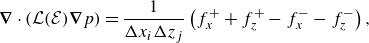 \begin{equation} \boldsymbol{\nabla} \cdot \left ({\mathcal{L}}({\mathcal{E}})\boldsymbol{\nabla} p\right ) = \frac {1}{\Delta x_{i}\Delta z_{j}}\left (f_{x}^{+}+f_{z}^{+}-f_{x}^{-}-f_{z}^{-}\right ), \end{equation}
where the fluxes are upwinded in the
 $z$
-direction, giving
$z$
-direction, giving
 \begin{gather} f_x^\pm \approx \Delta z_j\left .\left (\!{\mathcal{L}}\frac {\partial p}{\partial x}\!\right )\right |_{i+1/2,j} \approx \pm \Delta z_j\frac {\Delta x_{i\pm 1}{\mathcal{L}}(E_{i,j})+\Delta x_{i}{\mathcal{L}}(E_{i\pm 1,j})}{\Delta x_i + \Delta x_{i\pm 1}}\left (\!\frac {P_{i\pm 1,j}-P_{i,j}}{(\Delta x_i+\Delta x_{i\pm 1})/2}\!\right)\kern2.5pt,\end{gather}
 \begin{gather} f_z^+ \approx \Delta x_i{\mathcal{L}}(E_{i,j})\left .\frac {\partial p}{\partial z}\right |_{i,j+1/2}\approx \Delta x_i{\mathcal{L}}(E_{i,j})\left (\frac {P_{i,j+1}-P_{i,j}}{(\Delta z_{j+1}+\Delta z_j)/2}\right)\kern-2.5pt,\end{gather}
 \begin{gather} f_z^- \approx \Delta x_i{\mathcal{L}}(E_{i,j-1})\left .\frac {\partial p}{\partial z}\right |_{i,j-1/2}\approx \Delta x_i{\mathcal{L}}(E_{i,j-1})\left (\frac {P_{i,j}-P_{i,j-1}}{(\Delta z_{j}+\Delta z_{j-1})/2}\right)\kern-2.5pt. \end{gather}
The same discretisation is used for the flux,
 $\mathcal{S}({\mathcal{E}})\boldsymbol{\nabla} p$
, in the heat equation, simply replacing
$\mathcal{S}({\mathcal{E}})\boldsymbol{\nabla} p$
, in the heat equation, simply replacing
 ${\mathcal{L}}$
with
${\mathcal{L}}$
with
 $\mathcal{S}$
. We then flatten the grid via
$\mathcal{S}$
. We then flatten the grid via
 $\{\boldsymbol{x}_I=\boldsymbol{x}_{i,j}: \text{ where } 1\leqslant I\equiv N(j-1)+i\leqslant NM\}$
and obtain matrix equations for the vectors
$\{\boldsymbol{x}_I=\boldsymbol{x}_{i,j}: \text{ where } 1\leqslant I\equiv N(j-1)+i\leqslant NM\}$
and obtain matrix equations for the vectors
 $\boldsymbol{E}= ( E_{N+1}, E_{N+2}, \ldots , E_{N(M-1)} )$
and
$\boldsymbol{E}= ( E_{N+1}, E_{N+2}, \ldots , E_{N(M-1)} )$
and
 $\boldsymbol{P}= (P_{N+1},P_{N+2},\ldots ,P_{N(M-1)} )$
, where
$\boldsymbol{P}= (P_{N+1},P_{N+2},\ldots ,P_{N(M-1)} )$
, where
 $E_I={\mathcal{E}}(\boldsymbol{x}_I)$
and
$E_I={\mathcal{E}}(\boldsymbol{x}_I)$
and
 $P_I$
defined similarly. Note that
$P_I$
defined similarly. Note that
 $E_{1}=E_2=\ldots =E_N=0$
and
$E_{1}=E_2=\ldots =E_N=0$
and
 $P_1=P_2=\ldots =P_N=1$
by the boundary conditions at
$P_1=P_2=\ldots =P_N=1$
by the boundary conditions at
 $z=0$
and
$z=0$
and
 $P_{N(M-1)+1}=P_{N(M-1)+2}=\ldots =P_{NM}=0$
by the boundary condition at
$P_{N(M-1)+1}=P_{N(M-1)+2}=\ldots =P_{NM}=0$
by the boundary condition at
 $z=1$
. There is no equivalent boundary condition for
$z=1$
. There is no equivalent boundary condition for
 ${\mathcal{E}}$
at
${\mathcal{E}}$
at
 $z=1$
, as appropriate given the hyperbolic nature of the equation, and so
$z=1$
, as appropriate given the hyperbolic nature of the equation, and so
 $E_{N(M-1)+1}, E_{N(M-1)+2}, \ldots , E_{NM}$
are never determined and do not enter the discretised equations due to the flux being up-winded in the
$E_{N(M-1)+1}, E_{N(M-1)+2}, \ldots , E_{NM}$
are never determined and do not enter the discretised equations due to the flux being up-winded in the
 $z$
-direction (see A5). The discrete equations take the form
$z$
-direction (see A5). The discrete equations take the form
 \begin{align}\frac {1}{\Pi }\dot { E}_I&= A_{IJK}\mathcal{S}({ E}_J){ P}_K + a_{IJ}\mathcal{S}({ E}_J)+\frac {1}{\Pi }{\mathcal{C}}(E_I)\equiv F_I(\boldsymbol{E},\boldsymbol{P}), \end{align}
 \begin{align} 0 &=A_{IJK}{\mathcal{L}}({ E}_J){ P}_K+ a_{IJ}{\mathcal{L}}({ E}_J)+ b_{IJ}{ P}_J\equiv G_I(\boldsymbol{E},\boldsymbol{P}), \end{align}
where
 $A_{IJK}$
is a sparse third-order tensor arising from the flux terms, and
$A_{IJK}$
is a sparse third-order tensor arising from the flux terms, and
 $a_{IJ}$
and
$a_{IJ}$
and
 $b_{IJ}$
are sparse matrices arising from the boundary conditions at
$b_{IJ}$
are sparse matrices arising from the boundary conditions at
 $z=1$
and
$z=1$
and
 $z=0$
, respectively. The no-flux conditions at
$z=0$
, respectively. The no-flux conditions at
 $x=0, L_x$
are imposed by setting the fluxes,
$x=0, L_x$
are imposed by setting the fluxes,
 $f_x^\pm$
, to zero, and thus these boundary conditions do not contribute additional terms to the equations.
$f_x^\pm$
, to zero, and thus these boundary conditions do not contribute additional terms to the equations.
Since the nonlinear functions of
 ${\mathcal{E}}$
are known analytically, the Jacobian of the system can be written down explicitly, given in block form by
${\mathcal{E}}$
are known analytically, the Jacobian of the system can be written down explicitly, given in block form by
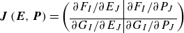 \begin{align} \boldsymbol{J} \left(\boldsymbol{E},\boldsymbol{P} \right)&= \left (\displaystyle \begin{array}{c|c} \partial F_I/\partial E_J & \partial F_I/\partial P_J \\[4pt] \hline \partial G_I/\partial E_J & \partial G_I/\partial P_J \end{array} \right ) \end{align}
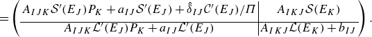 \begin{align} &=\left (\begin{array}{c|c} A_{IJK}\mathcal{S}'(E_J)P_K + a_{IJ}\mathcal{S}'(E_J)+\hat {\delta }_{IJ}{\mathcal{C}}'(E_J)/\Pi & A_{IKJ}\mathcal{S}(E_K) \\[4pt] \hline A_{IJK}{\mathcal{L}}'(E_J)P_K + a_{IJ}{\mathcal{L}}'(E_J) & A_{IKJ}{\mathcal{L}}(E_K)+b_{IJ} \end{array}\right ). \end{align}
Here,
 $K$
is summed over, but
$K$
is summed over, but
 $I$
and
$I$
and
 $J$
are not, and
$J$
are not, and
 $\hat {\delta }_{IJ}$
represents the Kronecker-delta function. This Jacobian is used throughout the numerical procedures: for Newton iterations when solving directly for the steady state,
$\hat {\delta }_{IJ}$
represents the Kronecker-delta function. This Jacobian is used throughout the numerical procedures: for Newton iterations when solving directly for the steady state,
 $F_I(\boldsymbol{E},\boldsymbol{P})=G_I(\boldsymbol{E},\boldsymbol{P})=0$
; for time-stepping of the advection equation (A7) using a fourth-order, five-stage Rosenbrock method (Roche Reference Roche1987); and in determining the linear stability of steady solutions to perturbations of the form
$F_I(\boldsymbol{E},\boldsymbol{P})=G_I(\boldsymbol{E},\boldsymbol{P})=0$
; for time-stepping of the advection equation (A7) using a fourth-order, five-stage Rosenbrock method (Roche Reference Roche1987); and in determining the linear stability of steady solutions to perturbations of the form
 ${ (\boldsymbol{E},\boldsymbol{P})}={ (\boldsymbol{E}_0,\boldsymbol{P}_0)}+{ (\boldsymbol{E}',\boldsymbol{P}')}e^{\sigma t}$
, for which the modes and corresponding growth-rates are found from the generalised eigenvalue problem:
${ (\boldsymbol{E},\boldsymbol{P})}={ (\boldsymbol{E}_0,\boldsymbol{P}_0)}+{ (\boldsymbol{E}',\boldsymbol{P}')}e^{\sigma t}$
, for which the modes and corresponding growth-rates are found from the generalised eigenvalue problem:
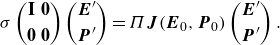 \begin{equation} \sigma \begin{pmatrix} \textbf{I} & \textbf{0} \\[4pt] \textbf{0} & \textbf{0} \end{pmatrix} \begin{pmatrix} { \boldsymbol{E}'} \\[4pt] { \boldsymbol{P}'} \end{pmatrix} = \Pi \boldsymbol{J}({ \boldsymbol{E}_0}, { \boldsymbol{P}_0}) \begin{pmatrix} { \boldsymbol{E}'} \\[4pt] { \boldsymbol{P}'} \end{pmatrix}. \end{equation}
All of these procedures are carried out in MATLAB (The MathWorks Inc. 2023a , b ), employing algorithms for large sparse arrays.
Appendix B. Comparison of averaging approaches
In this appendix, we make a quantitative comparison between the results of our heat-balance averaging and the approaches of Helfrich (Reference Helfrich1995), Wylie & Lister (Reference Wylie and Lister1995) and Morris (Reference Morris1996). We first compare the critical values of
 $\gamma$
in the uniform geometry, we denote
$\gamma$
in the uniform geometry, we denote
 $\gamma _c$
,
$\gamma _c$
,
 $\gamma _{3d}$
and
$\gamma _{3d}$
and
 $\gamma _\infty$
, as discussed in § 3.1. Not all of these are reported for the exponential viscosity function in all studies. Helfrich (Reference Helfrich1995) reports a value of
$\gamma _\infty$
, as discussed in § 3.1. Not all of these are reported for the exponential viscosity function in all studies. Helfrich (Reference Helfrich1995) reports a value of
 $\gamma _c=3.03$
for their averaging, while the unaveraged system first exhibits multiplicity of steady states at a larger value (
$\gamma _c=3.03$
for their averaging, while the unaveraged system first exhibits multiplicity of steady states at a larger value (
 $\gamma _c=5.19$
reported by Morris Reference Morris1996 and
$\gamma _c=5.19$
reported by Morris Reference Morris1996 and
 $\gamma _c=5.25$
reported by Wylie & Lister Reference Wylie and Lister1995). Thus, the value of
$\gamma _c=5.25$
reported by Wylie & Lister Reference Wylie and Lister1995). Thus, the value of
 $\gamma _c=4.8$
, found using our heat balance averaging, agrees better with the value for the unaveraged case than when employing the Darcy averaging, but still underestimates the critical viscosity ratio. For the unaveraged model with the exponential viscosity model,
$\gamma _c=4.8$
, found using our heat balance averaging, agrees better with the value for the unaveraged case than when employing the Darcy averaging, but still underestimates the critical viscosity ratio. For the unaveraged model with the exponential viscosity model,
 $\gamma _{3d}\approx 5.5$
(see Morris Reference Morris1996, figures 5 and 6) and
$\gamma _{3d}\approx 5.5$
(see Morris Reference Morris1996, figures 5 and 6) and
 $\gamma _\infty =5.78$
(Morris Reference Morris1996), compared with the values
$\gamma _\infty =5.78$
(Morris Reference Morris1996), compared with the values
 $\gamma _{3d}\approx 5.2$
and
$\gamma _{3d}\approx 5.2$
and
 $\gamma _\infty \approx 5.4$
for our system. Thus, as well as reproducing the behaviour qualitatively, the heat balance averaging does not significantly underestimate the critical values of the viscosity ratio at which the system changes behaviour (compared with say the Darcy averaging of Helfrich Reference Helfrich1995).
$\gamma _\infty \approx 5.4$
for our system. Thus, as well as reproducing the behaviour qualitatively, the heat balance averaging does not significantly underestimate the critical values of the viscosity ratio at which the system changes behaviour (compared with say the Darcy averaging of Helfrich Reference Helfrich1995).
Nonetheless, the approximation of the temperature field by (2.10) does introduce quantitative differences from the unaveraged system. This is demonstrated in figure 13(a), which shows the steady-state solution curve for
 $\gamma =5.5$
, calculated with the Darcy averaging of Helfrich (Reference Helfrich1995), the unaveraged approach of Wylie & Lister (Reference Wylie and Lister1995) and Morris (Reference Morris1996), and the heat balance method detailed in § 2.1. All three approaches agree at low
$\gamma =5.5$
, calculated with the Darcy averaging of Helfrich (Reference Helfrich1995), the unaveraged approach of Wylie & Lister (Reference Wylie and Lister1995) and Morris (Reference Morris1996), and the heat balance method detailed in § 2.1. All three approaches agree at low
 $\Pi$
and
$\Pi$
and
 $Q$
, where the majority of the fissure has a uniform cold temperature across its width, but differ elsewhere. The origin of the discrepancies can be understood by considering the approximations to the temperature profile. Figure 13(b) shows example across-channel temperature profiles for the three models at the same average temperature. When the fluid is hot and the temperature profile is significantly non-uniform across the channel, the averaging of Helfrich (Reference Helfrich1995) tends to underestimate the temperature gradient at the wall (since it does not account for thin thermal boundary layers). As a result, the material cools less quickly and the dimensionless pressure drop at which the slow branch joins the intermediate branch is underestimated by this averaging. More dramatically, the flux on the fast branch is significantly overestimated. By contrast, the parabolic approximation to the temperature profile, (2.10), tends to overestimate the heat flux to the walls, and so the fold bifurcations happen at larger
$Q$
, where the majority of the fissure has a uniform cold temperature across its width, but differ elsewhere. The origin of the discrepancies can be understood by considering the approximations to the temperature profile. Figure 13(b) shows example across-channel temperature profiles for the three models at the same average temperature. When the fluid is hot and the temperature profile is significantly non-uniform across the channel, the averaging of Helfrich (Reference Helfrich1995) tends to underestimate the temperature gradient at the wall (since it does not account for thin thermal boundary layers). As a result, the material cools less quickly and the dimensionless pressure drop at which the slow branch joins the intermediate branch is underestimated by this averaging. More dramatically, the flux on the fast branch is significantly overestimated. By contrast, the parabolic approximation to the temperature profile, (2.10), tends to overestimate the heat flux to the walls, and so the fold bifurcations happen at larger
 $\Pi$
than in the unaveraged system. The flux on the fast branch (large
$\Pi$
than in the unaveraged system. The flux on the fast branch (large
 $\Pi$
and
$\Pi$
and
 $Q$
) agrees with the unaveraged model much more closely than when employing the averaging of Helfrich (Reference Helfrich1995), since the variation of the viscosity across the channel is included in the model, and the assumed temperature profile is able to more closely represent the true profile when the fluid is at the eruption temperature across most of the channel, with thermal boundary layers at the walls. As discussed in § 3.3, the strength of geometrically driven flow focussing is largely controlled by the relative magnitude of fluxes on the fast and slow branches, and so capturing this is particularly important in the current study.
$Q$
) agrees with the unaveraged model much more closely than when employing the averaging of Helfrich (Reference Helfrich1995), since the variation of the viscosity across the channel is included in the model, and the assumed temperature profile is able to more closely represent the true profile when the fluid is at the eruption temperature across most of the channel, with thermal boundary layers at the walls. As discussed in § 3.3, the strength of geometrically driven flow focussing is largely controlled by the relative magnitude of fluxes on the fast and slow branches, and so capturing this is particularly important in the current study.
Diagrams of the finite volume grid used for the numerical solutions. (a) Diagram showing layout of cells. (b) Close up of a single stencil, showing direction of fluxes into and out of a given cell.
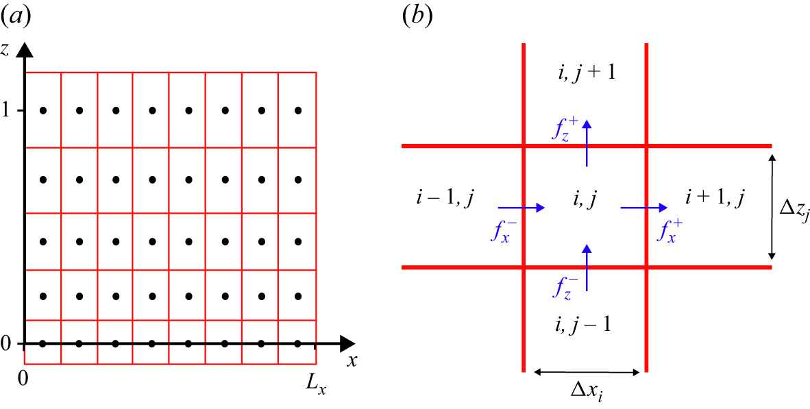
(a) Steady-state dimensionless flux per unit length,
 $Q$
, against dimensionless pressure drop,
$Q$
, against dimensionless pressure drop,
 $\Pi$
, for the uniform geometry,
$\Pi$
, for the uniform geometry,
 $h=1$
, and
$h=1$
, and
 $\gamma =5.5$
(as in figure 2). Solution curves are shown for the unaveraged approach of Morris (Reference Morris1996) (solid), the Darcy averaging employed by Helfrich (Reference Helfrich1995) (dotted) and the heat balance averaging detailed in § 2.1 (dashed). (b) Example across-channel temperature profiles,
$\gamma =5.5$
(as in figure 2). Solution curves are shown for the unaveraged approach of Morris (Reference Morris1996) (solid), the Darcy averaging employed by Helfrich (Reference Helfrich1995) (dotted) and the heat balance averaging detailed in § 2.1 (dashed). (b) Example across-channel temperature profiles,
 $T(y)$
. The solid curves show two temperature profiles that occur at different points along the channel in the unaveraged model of Morris (Reference Morris1996). These profiles were calculated using the numerical method detailed in Appendix B of Morris (Reference Morris1996), and are taken at the locations
$T(y)$
. The solid curves show two temperature profiles that occur at different points along the channel in the unaveraged model of Morris (Reference Morris1996). These profiles were calculated using the numerical method detailed in Appendix B of Morris (Reference Morris1996), and are taken at the locations
 $s=0.1$
(top) and
$s=0.1$
(top) and
 $s=0.6$
(bottom) in the notation of their appendix. Dashed lines show corresponding temperature profiles from the approximation (2.10), giving the same average temperature across the gap. The dotted lines show the sinusoidal profile giving the same average, as used by Helfrich (Reference Helfrich1995) in modelling the heat flux at the wall (but not the variation of viscosity across the channel).
$s=0.6$
(bottom) in the notation of their appendix. Dashed lines show corresponding temperature profiles from the approximation (2.10), giving the same average temperature across the gap. The dotted lines show the sinusoidal profile giving the same average, as used by Helfrich (Reference Helfrich1995) in modelling the heat flux at the wall (but not the variation of viscosity across the channel).
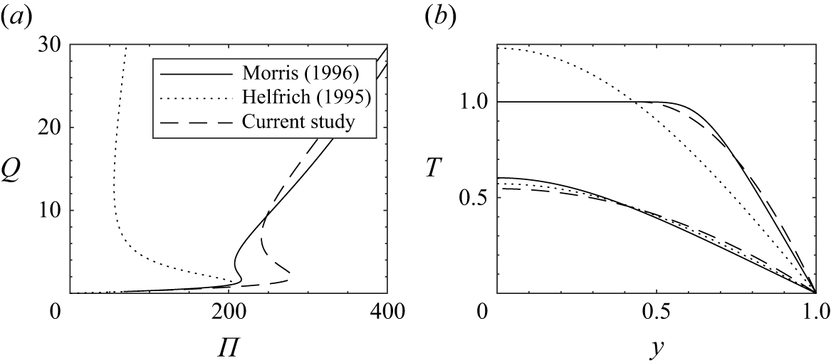
In figure 14, we include some results for a non-uniform geometry and the ‘unaveraged’ model of Wylie & Lister (Reference Wylie and Lister1995) for comparison with the results of the heat balance averaging. Panels (a)–(c) show the steady-state curves for the sinusoidal geometries with
 $A=0.05$
and
$A=0.05$
and
 $\lambda =2$
, 1 and 0.4, and
$\lambda =2$
, 1 and 0.4, and
 $\gamma =5.5$
, to be compared with the middle column of figure 4, while panel (d) corresponds to figure 5(c). The qualitative behaviour is very similar, with the unstable middle branch of the solution curve being replaced with a stable, flow-focussed branch. The range of
$\gamma =5.5$
, to be compared with the middle column of figure 4, while panel (d) corresponds to figure 5(c). The qualitative behaviour is very similar, with the unstable middle branch of the solution curve being replaced with a stable, flow-focussed branch. The range of
 $\Pi$
that is spanned by this branch is shorter and is shifted to lower values of
$\Pi$
that is spanned by this branch is shorter and is shifted to lower values of
 $\Pi$
, as anticipated from a comparison of the locations of the fold bifurcations for the uniform geometry (see figure 13
a). The degree of flux focussing, indicated by the scaled surface flux ratio,
$\Pi$
, as anticipated from a comparison of the locations of the fold bifurcations for the uniform geometry (see figure 13
a). The degree of flux focussing, indicated by the scaled surface flux ratio,
 $\tilde {Q}_r$
, is also not as large as for the heat balance averaging, but is still significantly stronger than that obtained from steady fingered solutions, typically exceeding a factor of 4. We note that, since
$\tilde {Q}_r$
, is also not as large as for the heat balance averaging, but is still significantly stronger than that obtained from steady fingered solutions, typically exceeding a factor of 4. We note that, since
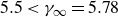 $5.5\lt \gamma _\infty =5.78$
for the unaveraged system (Morris Reference Morris1996), at this value of
$5.5\lt \gamma _\infty =5.78$
for the unaveraged system (Morris Reference Morris1996), at this value of
 $\gamma$
, the region of the solution branch which becomes unstable to the fingering instability is rather limited. We were unable to find any steady flow-focussed states for the uniform geometry at this parameter value, with the unstable solutions instead continuing to evolve onto the fast branch, as observed by Wylie & Lister (Reference Wylie and Lister1995). Thus, in this case, the non-uniform geometry provides a mechanism for the existence of steady flow-focussed solutions which are otherwise absent in the case of the uniform geometry. We further note that, in this case, there are no periodic solutions, which also relates to the absence of steady fingered states in the uniform geometry at this viscosity ratio, since the periodic orbits arise from oscillations between different fingered states (see § 3.4).
$\gamma$
, the region of the solution branch which becomes unstable to the fingering instability is rather limited. We were unable to find any steady flow-focussed states for the uniform geometry at this parameter value, with the unstable solutions instead continuing to evolve onto the fast branch, as observed by Wylie & Lister (Reference Wylie and Lister1995). Thus, in this case, the non-uniform geometry provides a mechanism for the existence of steady flow-focussed solutions which are otherwise absent in the case of the uniform geometry. We further note that, in this case, there are no periodic solutions, which also relates to the absence of steady fingered states in the uniform geometry at this viscosity ratio, since the periodic orbits arise from oscillations between different fingered states (see § 3.4).
Example steady-state results for the ‘unaveraged’ model of Wylie & Lister (Reference Wylie and Lister1995) with
 $\gamma =5.5$
and the sinusoidal geometry with
$\gamma =5.5$
and the sinusoidal geometry with
 $A=0.05$
. (a) Steady-state solution curves,
$A=0.05$
. (a) Steady-state solution curves,
 $Q$
as a function of
$Q$
as a function of
 $\Pi$
, as in figure 4, with colour corresponding to the scaled surface flux ratio,
$\Pi$
, as in figure 4, with colour corresponding to the scaled surface flux ratio,
 $\tilde {Q}_r$
, as shown in the logarithmic colour bar on the right. The three coloured curves are for geometrical wavelengths,
$\tilde {Q}_r$
, as shown in the logarithmic colour bar on the right. The three coloured curves are for geometrical wavelengths,
 $\lambda =0.4, 1$
and
$\lambda =0.4, 1$
and
 $2$
(increasing in the direction shown) and the black dotted curve shows the steady-state solution curve for the uniform geometry,
$2$
(increasing in the direction shown) and the black dotted curve shows the steady-state solution curve for the uniform geometry,
 $A=0$
. The corresponding results for the heat balance averaging can be found in the middle curve of each panel in figure 4. (b) Contour plot of scaled surface flux ratio,
$A=0$
. The corresponding results for the heat balance averaging can be found in the middle curve of each panel in figure 4. (b) Contour plot of scaled surface flux ratio,
 $\tilde {Q}_r$
, as a function of dimensionless pressure drop and wavelength, as in figure 5(c). The black contours are plotted at
$\tilde {Q}_r$
, as a function of dimensionless pressure drop and wavelength, as in figure 5(c). The black contours are plotted at
 $\tilde {Q}_r=4$
and 8. See table 2 for other parameters used in these solutions.
$\tilde {Q}_r=4$
and 8. See table 2 for other parameters used in these solutions.
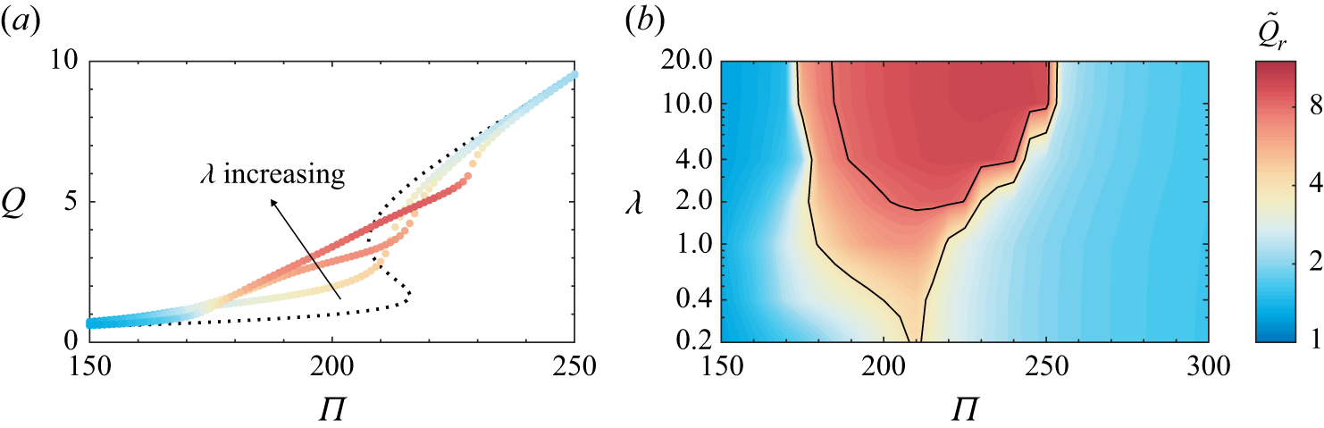


 Open access