2.1. The second-order p.d.f. of $\zeta$ derived from the moment generating function

The moment generating function of $\zeta$, $M_\zeta (s)$, is defined as

(2.2)\begin{equation} M_\zeta(s) \equiv \langle \exp(\zeta s) \rangle, \end{equation}

where $s$ is a dimensionless (possibly complex) variable and $\langle {\cdot } \rangle$ denotes the expectation operator. Letting $p(\zeta )$ denote the p.d.f. of $\zeta$ and substituting $i s$ for $s$ gives the integral equation

(2.3)\begin{equation} M_\zeta({\rm i}s) = \int_{-\infty}^{\infty} \exp ({\rm i} \zeta s) p(\zeta) \,\mathrm{d}\zeta, \end{equation}

which is readily inverted for $p(\zeta )$ by means of the inverse Fourier transform

(2.4)\begin{equation} p(\zeta) = \frac{1}{2{\rm \pi}} \int_{-\infty}^{\infty} M_\zeta(is) \exp(- {\rm i}\zeta s) \,\mathrm{d} s. \end{equation}

Thus, it is seen that one way to obtain the p.d.f. of a random variable is through the inverse Fourier transform of its moment generating function. Now, to compute the moment generating function of $\zeta$, we make use of its power series form

(2.5)\begin{equation} M_\zeta(s) = \sum_{q = 0}^{\infty} \frac{s^q}{q!} \langle \zeta^q \rangle, \end{equation}

which can be derived by Taylor expanding the exponential function in (2.2) and exploiting the linearity of the expectation operator. To compute the moments we will consider the cases where $q$ is even and odd separately.

When $q$ is even we may write $q = 2m$, where $m$ is a non-negative integer, and hence

(2.6)\begin{equation} \langle \zeta^q \rangle = \langle \zeta^{2m} \rangle = \langle ( \zeta_1 + \zeta_2 )^{2m} \rangle \end{equation}

upon using (2.1). The binomial theorem then gives that

(2.7)\begin{equation} \langle \zeta^{q} \rangle = \sum_{n = 0}^{2m} {2m \choose n} \langle \zeta_1^{2m-n} \zeta_2^{n} \rangle, \end{equation}

where $(\begin{smallmatrix}{2m}\\ {n}\end{smallmatrix})$ is the $2m$ choose $n$ binomial coefficient. Assuming $\zeta _1$ to be a linear combination of sine waves with random, independent phases implies that any term containing an odd power of $\zeta _1$ vanishes. By additionally assuming their frequencies to be densely distributed, to second order in the wave steepness, we have

(2.8)\begin{equation} \langle \zeta^{q} \rangle = \langle \zeta_1^{2m} \rangle = \frac{(2m)!}{2^m m!} \langle \zeta_1^{2} \rangle^m = \frac{(2m)!}{2^m m!}, \end{equation}

where the second equality above may be shown to hold using arguments identical to those used by e.g. Reference Longuet-HigginsLH63 (see e.g. his p. 462) in addition to Song & Wu (Reference Song and Wu2000) or Klahn et al. (Reference Klahn, Madsen and Fuhrman2021a) (their § 4.1.1). The last equality follows from the fact that $\zeta$, by definition, has unit variance i.e. to second order $\langle \zeta ^2\rangle =\langle \zeta _1^2\rangle =1$. We note that the even moments are $O(1)$.

When $q$ is odd we may instead write $q = 2m+1$, and using the same arguments as above, we find that

(2.9)\begin{equation} \langle \zeta^q \rangle = \langle \zeta^{2m+1} \rangle = (2m+1) \langle \zeta_1^{2m} \zeta_2 \rangle \end{equation}

when keeping the terms consistent with the second-order approximation. Again using a calculation analogous to that of Song & Wu (Reference Song and Wu2000) (see their Appendix), this result may further be shown to be

(2.10)\begin{equation} \langle \zeta^{q} \rangle = \frac{(2m+1)!}{2^{m-1} (m-1)!} \frac{\mathcal{S}}{6}, \end{equation}

where it has been used that, to second order, the skewness is $\mathcal {S} \equiv \langle \zeta ^3\rangle =3\langle \zeta _1^2\zeta _2\rangle$, which we note is $O(\varepsilon )$. Combining the even and odd moments with the power series form of the moment generating function (2.5), and shifting indices in the odd terms, then gives

(2.11)\begin{equation} M_\zeta(s) = \sum_{q = 0}^{\infty} \frac{1}{q!} \left( \frac{s^2}{2} \right)^q \left( 1 + \frac{1}{6} \mathcal{S} s^3 \right) = \exp\left( \frac{s^2}{2} \right) \left( 1 + \frac{1}{6} \mathcal{S} s^3 \right). \end{equation}

It now follows from (2.4) that, to second order in the wave steepness, the moment generating function predicts the p.d.f. of the surface elevation to be

(2.12)\begin{equation} p(\zeta) = \frac{1}{2{\rm \pi}} \int_{-\infty}^{\infty} \exp \left(-\frac{1}{2} (s^2 + {\rm i} \zeta s) \right) \left(1 + \frac{1}{6} \mathcal{S} ({\rm i}s)^3 \right) \mathrm{d} s. \end{equation}

Upon integrating, the result is

(2.13)\begin{equation} p(\zeta) = \frac{1}{\sqrt{2{\rm \pi}}} \exp \left( - \frac{\zeta^2}{2} \right) \left( 1 + \frac{1}{6} \mathcal{S} (\zeta^3 - 3\zeta) \right). \end{equation}

This concludes our derivation of the p.d.f. of the surface elevation based on the moment generating function.

Interestingly, the resulting expression for $p(\zeta )$ above was also found to second order by Reference Longuet-HigginsLH63, who based his derivation on the cumulant generating function, rather than the moment generating function utilized above. His derivation will be briefly reviewed and discussed further in § 3.

2.2. The second-order p.d.f. of $\zeta$ derived from the cumulant generating function

From the above it is seen that obtaining the p.d.f. of $\zeta$ from its moment generating function requires the calculation of an infinite number of moments. This is due to the fact that each moment, in general, consists of a first-order contribution, a second-order contribution and so on. In that regard utilizing the cumulant generating function of $\zeta$, $C_\zeta (s)$ is much simpler, as its terms are ordered in powers of $\varepsilon$. It is defined as

(2.14)\begin{equation} C_\zeta(s) \equiv \ln\left( M_\zeta(s) \right). \end{equation}

Moreover, the cumulants of $\zeta$ correspond directly to the coefficients $C_q$ in the Taylor expansion

(2.15)\begin{equation} C_\zeta(s) = \sum_{q = 1}^{\infty} \frac{C_q}{q!} s^q. \end{equation}

Upon insertion of the power series form of the moment generating function (2.5) into (2.14), and then Taylor expanding the logarithm, one finds that the first three cumulants are

(2.16a)$$\begin{gather} C_1 = \langle \zeta \rangle = 0, \end{gather}$$

(2.16b)$$\begin{gather}C_2 = \langle \zeta^2 \rangle - \langle \zeta \rangle^2 = 1, \end{gather}$$

(2.16c)$$\begin{gather}C_3 = \langle \zeta \rangle^3 - 3 \langle \zeta^2 \rangle\langle \zeta \rangle + 2 \langle \zeta \rangle^3 = \mathcal{S}, \end{gather}$$

and that all other cumulants are $O(\varepsilon ^2)$ or smaller. To second order in the wave steepness the cumulant generating function thus reads

(2.17)\begin{equation} C_\zeta(s) = \tfrac{1}{2}s^2 + \tfrac{1}{6}\mathcal{S}s^3. \end{equation}

Combining this result with (2.14) and (2.4) then implies that

(2.18)\begin{equation} p(\zeta) = \frac{1}{2{\rm \pi}} \int_{-\infty}^{\infty} \exp \left( -\frac{1}{2} s^2 + {\rm i}\zeta s + \frac{{\rm i}}{6} \mathcal{S} s^3 \right) \mathrm{d} s, \end{equation}

where it has been utilized that the sign of imaginary terms within the exponential may be freely reversed without modifying the integral. To work out the integral, we start by making a change of variables. Setting

(2.19)\begin{equation} s = \left( \frac{2}{\mathcal{S}}\right)^{1/3} \tau - \frac{{\rm i}}{\mathcal{S}} \end{equation}

transforms the integral to

(2.20)\begin{equation} p(\zeta) = \frac{1}{2{\rm \pi}} \left( \frac{2}{\mathcal{S}}\right)^{1/3} \exp \left( \frac{1}{3 \mathcal{S}^2} + \frac{\zeta}{\mathcal{S}}\right) \int_{-\infty + {\rm i}\gamma}^{\infty + {\rm i}\gamma} \exp \left( {\rm i} \left( \frac{\tau^3}{3} + \chi \tau \right) \right) \mathrm{d}\tau, \end{equation}

in which

(2.21)\begin{equation} \gamma = \frac{1}{2^{1/3} \mathcal{S}^{2/3}} \end{equation}

and

(2.22)\begin{equation} \chi = \left(\frac{2}{\mathcal{S}} \right)^{1/3} \left( \frac{1}{2 \mathcal{S}} + \zeta \right)\end{equation}

are introduced for notational convenience. Now, (2.20) is a contour integral in the complex plane with the contour being a straight line lying a distance $\gamma$ above the real line. However, as we will now show, the contour can be pushed down to the real line. To demonstrate this, consider the contour integral

(2.23)\begin{equation} \int_{\varGamma} \exp \left( {\rm i} \left( \frac{z^3}{3} + \chi z \right) \right) \mathrm{d} z = \sum_{n=1}^4 \underbrace{\int_{\varGamma_n} \exp \left( {\rm i} \left( \frac{z^3}{3} + \chi z \right) \right) \mathrm{d} z}_{I_n} \equiv \sum_{n=1}^4 I_n, \end{equation}

where the contour $\varGamma$, and its sub-contours, are defined in figure 1 and should be considered in the limit $R \rightarrow \infty$. Since the integrand is analytic, the residue theorem implies that the integral along $\varGamma$ is exactly zero (see e.g. Berg Reference Berg2013) for any value of $R$. Hence, if it can be proved that $I_2$ and $I_4$ vanish when $R$ becomes large, we will have shown that (2.20) may, in fact, be evaluated by integrating along the real line. Considering $I_2$ first, it is clear that

(2.24)\begin{equation} |I_2|= \left| \int_{\varGamma_2} \exp \left( {\rm i} \left( \frac{z^3}{3} + \chi z \right) \right) \mathrm{d} z \right| \leqslant \int_{\varGamma_2} \left| \exp \left( {\rm i} \left( \frac{z^3}{3} + \chi z \right) \right) \right| \mathrm{d} z. \end{equation}

If we parameterize $\varGamma _2$ letting $z(\delta ) = R + i\gamma (1-\delta )$ with $0 \leqslant \delta \leqslant 1$, and utilize the fact that $\gamma$ is positive, this leads directly to

(2.25)\begin{equation} |I_2|\leqslant\gamma \int_{0}^{1} \exp \left( -\gamma \left( R^2 + \chi\right) (1-\delta) + \frac{\gamma^3}{3}(1-\delta)^3\right) \mathrm{d}\delta. \end{equation}

Now, since $(1-\delta )^3\leqslant (1-\delta )$ over the range of $\delta$ considered, we may replace the former with the latter in the final (positive) term within the exponential. This then yields that

(2.26)\begin{equation} |I_2|\leqslant \gamma \int_{0}^{1} \exp \left( -\gamma \left( R^2 + \chi - \frac{\gamma^2}{3}\right) (1-\delta) \right) \mathrm{d}\delta, \end{equation}

and working out the integral then gives that

(2.27)\begin{equation} |I_2| \leqslant \frac{1-\exp(-\gamma(R^2+\chi-\gamma^2/3))}{R^2+\chi-\gamma^2/3}, \end{equation}

and hence

(2.28)\begin{equation} |I_2| \leqslant\frac{1}{R^2 + \chi - \gamma^2/3}, \end{equation}

whose limit is zero as $R\to \infty$. We have thus shown that $I_2$ vanishes in this limit. As an identical argument can be used to show that $I_4$ also becomes negligible when $R$ becomes large, we do not present it here, but conclude that the contour in (2.23) can indeed be pushed down to the real line. Doing so yields

(2.29)\begin{equation} p(\zeta) = \frac{1}{2{\rm \pi}} \left( \frac{2}{\mathcal{S}}\right)^{1/3} \exp \left( \frac{1}{3 \mathcal{S}^2} + \frac{\zeta}{\mathcal{S}}\right) \int_{-\infty}^{\infty } \exp \left( {\rm i} \left( \frac{\tau^3}{3} + \chi \tau \right) \right) \mathrm{d}\tau. \end{equation}

Since the argument of the exponential function in the integrand is an odd function of $\tau$, using the polar form of the integrand gives

(2.30)\begin{equation} p(\zeta) = \frac{1}{\rm \pi} \left( \frac{2}{\mathcal{S}}\right)^{1/3} \exp \left( \frac{1}{3 \mathcal{S}^2} + \frac{\zeta}{\mathcal{S}}\right) \int_{0}^{\infty } \cos \left( \frac{\tau^3}{3} + \chi \tau \right) \mathrm{d}\tau. \end{equation}

This may be equivalently written as

(2.31)\begin{equation} p(\zeta) = \left( \frac{2}{\mathcal{S}}\right)^{1/3} \exp \left( \frac{1}{3 \mathcal{S}^2} + \frac{\zeta}{\mathcal{S}}\right) \text{Ai} (\chi), \end{equation}

where

(2.32)\begin{equation} \text{Ai}(\chi)\equiv\frac{1}{\rm \pi}\int_0^\infty \cos\left(\frac{\tau^3}{3}+\chi\tau\right)\mathrm{d}\tau \end{equation}

defines the integral representation of the Airy function of the first kind, which is explicitly available in most any mathematical software or programming language.

Figure 1.

The contour $\varGamma = \cup _{n = 1}^4 \varGamma _n$, which should be considered in the limit where $R$ tends to $\infty$. The arrows indicate the direction of integration along the segments.

The result found in (2.31) is new, and seemingly corresponds to the first time the second-order p.d.f. has been derived from the cumulant generating function, without resorting to any further approximation.

2.3. Asymptotic equivalence of the two approaches for small steepness

At first glance, the p.d.f.s derived from the moment (2.13) and cumulant generating functions (2.31) appear quite different. However, they are both second-order approximations of the exact p.d.f., and it is therefore natural to expect that they become equivalent in the limit of small wave steepness. In this section we demonstrate that this is indeed the case by showing that (2.31) reduces to (2.13) when $\varepsilon$ is small.

To do so, we start by noting that, when $\varepsilon$ is small, $\mathcal {S}$ becomes small, and hence $\chi$ becomes large. For large, positive and real arguments (see e.g. Abramowitz & Stegun Reference Abramowitz and Stegun1964) the asymptotic form of the Airy function is

(2.33)\begin{equation} \text{Ai}(\chi) \sim \frac{1}{2 {\rm \pi}^{1/2} \chi^{1/4}} \exp\left( - \frac{2}{3} \chi^{3/2} \right) \sum_{n = 0}^{\infty} \frac{ \left( -\frac{3}{4} \right)^n \, \varGamma \left(n + \frac{5}{6} \right) \varGamma \left(n + \frac{1}{6} \right)}{2{\rm \pi} n! \chi^{3n/2}}. \end{equation}

Since $\chi \sim \varepsilon ^{-4/3}$ in the limit $\varepsilon \rightarrow 0$, the $n$th term in the series is asymptotically of order $\varepsilon ^{2n}$. For consistency with the assumption made in the previous section, we only retain terms up to $O(\varepsilon )$, and by using that $\varGamma (5/6) \varGamma (1/6) = 2{\rm \pi}$, we obtain

(2.34)\begin{equation} \text{Ai}(\chi) = \frac{1}{2 {\rm \pi}^{1/2} \chi^{1/4}} \exp\left( - \frac{2}{3} \chi^{3/2} \right) + O(\varepsilon^2). \end{equation}

Now, a first-order Taylor series expansion in $\mathcal {S}$ of $(1 + 2 \mathcal {S} \zeta )^{-1/4}$ yields

(2.35)\begin{equation} \frac{1}{2 {\rm \pi}^{1/2} \chi^{1/4}} = \frac{1}{\sqrt{2{\rm \pi}}} \left(\frac{2}{\mathcal{S}} \right)^{-1/3} \left( 1 - \frac{1}{2} \mathcal{S} \zeta + O ( \varepsilon^2 ) \right). \end{equation}

Moreover, from a third-order Taylor series expansion of $(1 + 2 \mathcal {S} \zeta )^{3/2}$ it follows that

(2.36)\begin{align} \exp \left( -\frac{2}{3} \chi^{3/2} \right) & = \exp \left( - \frac{1}{3 \mathcal{S}^2} \left( 1 + 3 \mathcal{S} \zeta + \frac{3}{2} \mathcal{S}^2 \zeta^2 - \frac{1}{2} \mathcal{S}^3 \zeta^3 + O (\varepsilon^4) \right)\right) \nonumber\\ & = \exp \left( - \frac{1}{3 \mathcal{S}^2} - \frac{\zeta}{\mathcal{S}} - \frac{\zeta^2}{2} \right) \left( 1 + \frac{\mathcal{S}}{6} \zeta^3 + O (\varepsilon^2) \right). \end{align}

Hence, we may rewrite the asymptotic approximation of the Airy function as

(2.37)\begin{equation} \text{Ai}(\chi) = \frac{1}{\sqrt{2{\rm \pi}}} \left(\frac{2}{\mathcal{S}} \right)^{-1/3} \exp \left( - \frac{1}{3 \mathcal{S}^2} - \frac{\zeta}{\mathcal{S}} - \frac{\zeta^2}{2} \right) \left( 1 + \frac{\mathcal{S}}{6} (\zeta^3 - 3\zeta ) + O ( \varepsilon^2 ) \right). \end{equation}

Inserting this into (2.31), we then find that

(2.38)\begin{equation} p(\zeta) = \frac{1}{\sqrt{2{\rm \pi}}} \exp \left( -\frac{\zeta^2}{2} \right) \left( 1+\frac{\mathcal{S}}{6}(\zeta^3-3\zeta) + O (\varepsilon^2)\right), \end{equation}

which matches the result seen in (2.13). Thus, we have shown that the second-order results implied by the moment and cumulant generating functions are asymptotically equivalent in the limit of small wave steepness. Obviously, both reduce to the Gaussian (normal) distribution

(2.39)\begin{equation} p(\zeta) = \frac{1}{\sqrt{2{\rm \pi}}} \exp \left( -\frac{\zeta^2}{2} \right)\end{equation}

in the linear limit.

5.1. Removal of spurious oscillations in the negative tail

As shown in figure 2 (full line), for finite $\mathcal {S}$ and moderate to large, negative $\zeta$, the p.d.f. given in (2.31) results in spurious oscillations, and even negative probability densities. Such features can obviously be dismissed as non-physical. A semi-theoretical method for addressing the oscillations inherent in (2.31), valid for small but finite $\mathcal {S}$, will be developed in the present section, inspired by inspection of the Airy functions with negative arguments. For later use within this section, note that the Airy function of the second kind is defined by

(5.1)\begin{equation} \text{Bi}(\chi)\equiv\frac{1}{\rm \pi} \int_0^\infty\left[ \exp\left(-\frac{\tau^3}{3}+\chi\tau\right) +\sin\left(\frac{\tau^3}{3}+\chi\tau\right) \right]\mathrm{d}\tau. \end{equation}

To begin, both $\text {Ai}(\chi )$ (grey dashed line) and $\text {Bi}(\chi )$ (grey dotted line) are plotted in figure 4. It is additionally noted that the envelope of both Airy functions (with negative arguments) follows

(5.2)\begin{equation} \mbox{Ci}(\chi)\equiv [\text{Ai}(\chi)^2+\text{Bi}(\chi)^2]^{1/2}, \end{equation}

which is depicted as the full line in figure 4. The asymptotic limit as $\chi \to -\infty$, $\mbox {Ci}(\chi )\sim {\rm \pi}^{-1/2}(-\chi )^{-1/4}$, is also shown for completeness.

Figure 4.

Plot demonstrating the behaviour of the Airy functions $\text {Ai}(\chi )$ and $\text {Bi}(\chi )$, their envelope $\mbox {Ci}(\chi )$ as well as its asymptotic form $\mbox{Ci}(\chi)\sim{\rm \pi}^{-1/2}(-\chi)^{-1/4}$.

Inspired by the observations above, we propose the following as a suitable generalization of (2.31) for some practical purposes:

(5.3)\begin{equation} p(\zeta)= \left(\frac{2}{\mathcal{S}}\right)^{1/3} \exp\left[\frac{1}{3\mathcal{S}^2} + \frac{\zeta}{\mathcal{S}}\right] \mbox{Zi}\left(\chi\right), \end{equation}

wherein $\text {Ai}(\chi )$ has been replaced with

(5.4)\begin{equation} \mbox{Zi}(\chi)\equiv \begin{cases} \text{Ai}(\chi) & \text{for} \ \chi\geqslant\chi_0 \\ \mbox{Ci}(\chi) & \text{for} \ \chi<\chi_0. \end{cases}\end{equation}

To ensure smoothness of the modified p.d.f., we require that $\text {Ai}(\chi _0)=\mbox {Ci}(\chi _0)$ and $\text {Ai}^\prime (\chi _0)=\mbox {Ci}^\prime (\chi _0)$, both of which are satisfied at $\chi _0\approx -1.17371$, see figure 4. The modification above enables direct use of the $\text {Ai}(\chi )$ function for $\chi \geqslant \chi _0$, fully consistent with the theory from (2.31). Conversely, it switches to the envelope $\mbox {Ci}(\chi )$ for $\chi <\chi _0$, where the theoretical solution clearly breaks down.

To check the practical validity of (5.3), we plot the integral of the resulting p.d.f., as well as its first four statistical moments, vs the input skewness $\mathcal {S}$ in figure 5. All plotted quantities are thus of the general form

(5.5)\begin{equation} \int_{-\infty}^{\infty} \zeta^m p(\zeta)\,\mathrm{d}\zeta, \end{equation}

where $m=0, 1, \ldots, 4$, where each is normalized and/or vertically shifted as indicated in the figure legend, such that they should theoretically be equal to zero. It is seen that for all quantities plotted reasonable accuracy is maintained for say $\mathcal {S}\lesssim 0.2$. At the upper limit $\mathcal {S}=0.2$ the modified p.d.f. from (5.3) yields a mean of $-0.00015$, a variance of 1.0005, a skewness of 0.199 and a kurtosis of 3.007. These may be compared with their respective theoretical values of zero, unity, 0.2 (as input) and 3. It is emphasized that if the theoretical p.d.f. from (2.31) is maintained then the theoretical values are matched exactly, regardless of $\mathcal {S}$.

Figure 5.

Integral and statistical moments computed from the modified p.d.f. (5.3). All integrals have been shifted and/or normalized as indicated in the legend, such that plotted quantities should theoretically be zero.

An example using the modified p.d.f. defined in (5.3), now with $\mathcal {S}=0.2$ (again, the upper recommended limit), can be seen as the full black line in figure 6. This result can be compared with the previously discussed result based on (2.31), which is similarly plotted as the grey dashed line in figure 6. It is seen that the two are, by design, identical for positive and moderately negative $\zeta$. Importantly, (5.3) avoids any spurious non-physical oscillations for negative $\zeta$, which are erroneously exhibited by (2.31).

Figure 6.

Comparison of p.d.f.s from (5.3) (full line) and (2.31) (dashed line), with $\mathcal {S}=0.2$. Note the removal of spurious oscillations in the negative tail using (5.3).

To conclude: the theoretically derived new second-order p.d.f. corresponds to (2.31). Should it be desired, for weakly nonlinear cases having $\mathcal {S}\leqslant 0.2$, this may be replaced in practice with (5.3), which will remove spurious oscillations of the negative tail, while maintaining reasonably accurate statistical moments. The accuracy of the resulting p.d.f.s will be directly tested in § 6, where the limits in $\mathcal {S}$ suggested above will be strictly followed.

5.2. Numerical precision

Regarding practical issues, it should be finally mentioned that the evaluation of $\text {Ai}(\chi )$ can face problems associated with loss of numerical precision, particularly when considering cases having small $\mathcal {S}$. When making calculations in double precision we find that such issues can arise whenever this argument becomes $\chi >\chi _{thresh}\approx 108$, which will return zero, rather than an extremely small number (which in turn must be multiplied by an extremely large number stemming from the exponential function, see (2.31) or (5.3)). From the definition in (2.22), this issue will manifest in $p(\zeta )$ whenever

(5.6)\begin{equation} \zeta \gtrsim \frac{2^{2/3}\mathcal{S}^{4/3}\chi_{thresh}-1}{2\mathcal{S}}. \end{equation}

Fortunately, this issue is easily overcome in practice simply by ensuring that the argument $\chi$ is evaluated to high precision e.g. using vpi in Matlab or SetPrecision in Mathematica, and we recommend doing similarly for the argument of the exponential function for the sake of consistency. Such high-precision calculations have been utilized in all relevant plots presented throughout the present work. As an example implementation, a Matlab function pdfAiry.m evaluating the p.d.f. defined in (5.3) if $\mathcal {S}\leqslant 0.2$ and (2.31) otherwise is provided at the link indicated in the Data Availability section towards the end of the present paper.

6.1. Comparison with results from second-order irregular wave theory

As a first means of validation we will compare the new p.d.f.s against those generated from time series utilizing the directionally spread (third-order) irregular wave theory of Madsen & Fuhrman (Reference Madsen and Fuhrman2012), carried out to second order. (Note that some errors unfortunately appeared in their original publication, which are pointed out for clarity in Appendix A.) For validation purposes we will consider three cases, each based on a Joint North Sea Wave Project (JONSWAP) spectrum (Hasselmann et al. Reference Hasselmann1973)

(6.1)\begin{equation} S(\omega)=S_0\left(\frac{\omega}{\omega_p}\right)^{-5} \exp\Bigg(-\frac{5}{4}\left(\frac{\omega}{\omega_p}\right)^{-4}\Bigg)\gamma_s^{\exp\left(-(\omega/\omega_p-1)^2/(2\sigma_s^2)\right)}, \end{equation}

where $\omega$ is the angular frequency, $\omega _p$ is the peak angular frequency, $\gamma _s=3.3$ and $\sigma _s=0.07$ if $\omega <\omega _p$ and 0.09 otherwise. A cutoff frequency of $\omega _{c}=3\omega _p$ is utilized, such that $S(\omega >\omega _{c})=0$. The constant $S_0$ is defined such that the linearized spectrum satisfies

(6.2)\begin{equation} \int_0^\infty S(\omega) \,\mathrm{d}\omega = \sigma^2, \end{equation}

with second-order components added afterwards. The waves are directionally spread (utilizing single summation) based on

(6.3)\begin{equation} D(\theta)= \begin{cases} \dfrac{\varGamma(N_D/2+1)}{\sqrt{\rm \pi}(\varGamma(N_D+1)/2)} \cos^{N_D}(\theta) & \text{if} \ |\theta|\leqslant\dfrac{\rm \pi}{2} \\[10pt] 0 & \text{otherwise}, \end{cases} \end{equation}

where $\varGamma ({\cdot })$ denotes the gamma function and $N_D$ is the directional-spreading parameter, which governs the width of the directional spectrum.

All cases utilize a finite depth such that $k_ph=1.2$, where $k_p$ is the peak wavenumber, determined from the dispersion relation

(6.4)\begin{equation} \omega_p^2=g k_p\tanh{k_p h}, \end{equation}

and $h=70$ m is the water depth, with gravitational acceleration $g=9.81\ {\rm m}\ {\rm s}^{-2}$ such that the peak period is $T_p=16.8$ s. All cases utilize the directional-spreading parameter $N_D=50$. We will consider three cases representing storm conditions with linear steepness $\varepsilon =k_pH_{m0}/2=2k_p\sigma =0.10$, $0.15$ and $0.20$, where $H_{m0}$ is the spectral significant wave height. The primary purpose of the present comparisons is thus to test the performance of the new p.d.f.s for irregular wave fields having variable nonlinearity in finite depth. For each case numerous (${\approx }120\,000$) discrete time series segments have been independently generated, each spanning a duration $100T_p$, resolved with time step $\Delta t=T_p/20$. This means that, for each condition considered, approximately $6.4$ years of storm data are collectively generated and analysed. The resulting statistics (steepness $\varepsilon$, variance $\sigma ^2$, skewness $\mathcal {S}$ and kurtosis $\mathcal {K}$) are summarized in table 1.

Selected time series segments are exemplified in figure 7, corresponding to those containing the largest crest elevation generated for each case. Insets are provided on each panel, depicting a zoomed-in region surrounding the large crests. It is seen that these selected events contain isolated rogue waves, with crest elevations in the most extreme case generated reaching nearly $\zeta =8$. Interestingly, these extreme events are typically surrounded by otherwise rather ordinary conditions for the sea states considered, typically with $-3\leqslant \zeta \leqslant 3$. That the extreme waves would appear to have ‘come from nowhere’ seems consistent with anecdotal accounts often reported by mariners and as occasionally even measured. Note e.g. the qualitative similarity with the famous ‘New Year’ rogue wave, measured in the North Sea on 1 January 1995 from the Draupner oil platform (water depth $h=70$ m), similarly presented in figure 8. Based on analysis of this measured time series segment alone, the storm conditions there would correspond to $\sigma ^2\approx 8.9\ {\rm m}^2$, $k_ph\approx 1.2$ and $\varepsilon \approx 0.10$, similar to the input conditions leading to the event depicted in figure 7(a). (The close similarity in input for this case is intentional, as we were curious to see if similar peak events might indeed be generated stochastically using a second-order theory.)

Figure 7.

Example time series involving the largest crests (occurring at time $t=t_p$) generated by the irregular, directionally spread wave theory of Madsen & Fuhrman (Reference Madsen and Fuhrman2012) to second order. Insets depicting the region immediately surrounding the largest crest are added on each panel. Cases utilize $k_ph=1.2$ and $N_D=50$ coupled with linear steepness (a) $\varepsilon =0.10$, (b) 0.15 and (c) 0.20.

Figure 8.

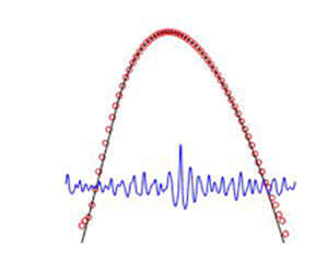
Time series segment containing the famous ‘New Year’ rogue wave measured from the Draupner oil platform in the North Sea on 1 January 1995.

For each case the numerous time series segments have been collectively analysed, with a $\zeta$ bin size corresponding to $0.2$, resulting in the three p.d.f.s (circles) shown in figure 9. Error bars are also included, estimated as $\pm p(\zeta )/\sqrt {N_b}$, where $N_b$ is the number of samples in each bin, following Onorato et al. (Reference Onorato2009). Also shown for comparison are the p.d.f.s from (i) the Gaussian distribution (dotted lines), (ii) Reference Longuet-HigginsLH63 (second order: dashed lines, third order: dashed-dotted lines) and (iii) the presently proposed p.d.f.s (full lines). In line with the recommendation made in § 5.1, the modified variant (5.3) is only utilized in the case where $\mathcal {S}\leqslant 0.2$ (figure 9a), whereas the theoretical p.d.f. (2.31) is utilized in figure 9(b,c). It is seen that the proposed new p.d.f. provides superior accuracy to both the Gaussian distributions (expected from linear theory), as well as those of Reference Longuet-HigginsLH63, especially in the positive tail. Somewhat remarkably, and as mentioned previously, even though effects of kurtosis are not at all accounted for, the present distribution even outperforms the third-order distribution of Reference Longuet-HigginsLH63. As should be expected from § 5.1, the distribution from (5.3) (figure 9a) is free of spurious oscillations in the negative tail, in contrast to those of Reference Longuet-HigginsLH63 or (2.31) which fail for roughly $\zeta <-3$. The comparison in figure 9(a) suggests that this modification provides similar accuracy for predicting the probability density of negative surface elevations as for positive ones, at least for cases having $\mathcal {S}\leqslant 0.2$ where it can be reasonably applied. Remaining differences between the generated data and the new p.d.f.s seem likely due to neglected third-order effects in the distribution (e.g. kurtosis). Obviously, none of the methods employed account for any effects of wave breaking on the p.d.f., although there is considerable evidence that these do not necessarily have a significant impact in the probability domain, see e.g. the discussion in Tayfun & Alkhalidi (Reference Tayfun and Alkhalidi2020).

Figure 9.

Comparison of p.d.f.s computed from the second-order directionally spread irregular wave theory of Madsen & Fuhrman (Reference Madsen and Fuhrman2012, referred to as MF12) (circles, with error bars) with (3.4) from Reference Longuet-HigginsLH63 (second order, dashed lines; third order, dashed-dotted lines) and the present work using (a) (5.3) and (b,c) (2.31) (full lines). Cases utilize $k_ph=1.2$ and $N_D=50$ coupled with (a) $\varepsilon =0.1007$, (b) 0.1524 and (c) 0.2057, with other statistical quantities given in table 1.

6.2. Comparison with results from fully nonlinear numerical simulations

As an additional means of validation, we will consider data generated utilizing the fully nonlinear pseudospectral Fourier–Legendre (PFL) potential flow simulation model of Klahn et al. (Reference Klahn, Madsen and Fuhrman2021c), as used previously by Klahn et al. (Reference Klahn, Madsen and Fuhrman2021a,Reference Klahn, Madsen and Fuhrmanb). This model is spectrally accurate in all three spatial directions and maintains good computational efficiency. This method makes use of an artificial lower boundary condition based on Nicholls (Reference Nicholls2011), with iterative solutions to the resulting Laplace equation utilizing a linearized preconditioner, following the strategy of Fuhrman & Bingham (Reference Fuhrman and Bingham2004). For full details on this model and features, see Klahn et al. (Reference Klahn, Madsen and Fuhrman2021a,Reference Klahn, Madsen and Fuhrmanb,Reference Klahn, Madsen and Fuhrmanc).

We simulate irregular, directionally spread wave fields, again based on JONSWAP spectra, with $k_ph=1.0$, $1.5$ and $\infty$ (deep water), now utilizing the directional-spreading parameter $N_D=2$. For all cases simulations utilize a large $2048\times 2048$ (horizontal) grid, coupled with $11$ points distributed in the vertical direction. The computational domain has lengths $L_x=100\lambda _p$ and $L_y=100(1+N_D)^{1/2}\lambda _p$, where $\lambda _p=2{\rm \pi} /k_p=275$ m, which provides similar resolution of wavelengths in both horizontal directions, following Klahn et al. (Reference Klahn, Madsen and Fuhrman2021a). Note that the resolution utilized implies that the spectrum is effectively cut off at $\omega _{c}\approx 4.86\omega _p$, see (3.24) of Klahn et al. (Reference Klahn, Madsen and Fuhrman2021a). The computational domains can be considered extremely large for such fully nonlinear simulations, covering a physical area corresponding to $28.2\ {\rm km} \times 48.8\ {\rm km}$. Starting with linearized initial conditions, the nonlinear terms are ramped to fully on over a duration of $10T_p$, following the same procedure described in Klahn et al. (Reference Klahn, Madsen and Fuhrman2021a,Reference Klahn, Madsen and Fuhrmanb), and then continued for a total duration of $100T_p$. The characteristic wave steepness for the linearized initial conditions are set according to $\varepsilon = \varepsilon _0\tanh (0.8863k_ph)$, where $\varepsilon _0 = 0.15$ is a deep water ‘equivalent steepness’. This ensures that, for a given $\varepsilon _0$, cases in any $k_ph$ will have roughly the same degree of nonlinearity, relative to the maximum steepness criterion of Battjes (Reference Battjes1974). The primary purpose of the present tests is thus to compare the performance of the new p.d.f.s in irregular wave fields having similar nonlinearity, but with variable dimensionless water depth. Note that above the steepness $\varepsilon _0=0.15$ it becomes difficult to maintain stable nonlinear statistics, as shown e.g. in figure 2(a) of Klahn et al. (Reference Klahn, Madsen and Fuhrman2021b). This is due to dissipative effects introduced through filtering, which is necessary for stability purposes when extremely steep (potentially breaking) waves are encountered. The time step is set such that $\Delta t=T_p/50$. For each case, we have carried out the time integration with five different initial conditions, with the phase of each wave component determined randomly. Each simulation considered requires several months of simulation time on a single processor. The resulting statistics (steepness $\varepsilon$, variance $\sigma ^2$, skewness $\mathcal {S}$ and kurtosis $\mathcal {K}$), based on data accumulated from all five simulations of each case at time $t=50T_p$, are summarized in table 2. Note that at this time the nonlinear wave fields can be considered well developed, with reasonably stable statistics, as established in previous simulations performed by Klahn et al. (Reference Klahn, Madsen and Fuhrman2021a,Reference Klahn, Madsen and Fuhrmanb).

An example snapshot of the computational line in $x$ containing the largest rogue wave peak elevation generated at time $t=50T_p$ from the simulated case with $k_ph=1.5$ is depicted in figure 10. Reasonable similarity with the time series from figures 7(a) and 8 can be there observed, with the free surface again reaching $\zeta \approx 6$. A small three-dimensional segment of the simulated large domain containing this rogue wave is likewise provided in figure 11, as an example.

Figure 10.

Example free surface elevation along the line containing the largest crest generated by the fully nonlinear wave model of Klahn et al. (Reference Klahn, Madsen and Fuhrman2021c) for the case with $k_ph=1.5$, $N_D=2$ and $\varepsilon =0.1270$. The inset depicts a zoomed-in region immediately surrounding the largest crest. Variable $x_p$ denotes the $x$ position of the highest crest peak.

Figure 11.

Snapshot of the surface elevation in the vicinity of the largest rogue wave crest generated by the fully nonlinear model of Klahn et al. (Reference Klahn, Madsen and Fuhrman2021c) for the case with $k_ph=1.5$, $N_D=2$ and $\varepsilon =0.1270$. The horizontal axes are to scale, whereas the vertical axis is exaggerated by a factor of two. The horizontal area shown is $4\lambda _p\times 4\lambda _p$.

The resulting p.d.f.s for the surface elevations accumulated from the fully nonlinear simulations for all three cases are presented as circles (with error bars, computed as previously described) in figure 12. For each case considered it is seen that isolated rogue waves having surface elevations reaching up to the previously mentioned $\zeta \approx 6$ have been generated in each case. As references the Gaussian distribution, as well as those from Reference Longuet-HigginsLH63 (both second and third order) are additionally shown in this figure. Good accuracy is confirmed with the present method utilizing (2.31) (figure 12a) and (5.3) (figure 12b,c as $\mathcal {S}\leqslant 0.2$) (full lines). The heavy positive tail associated with the present method is again evident, and is closer to the data than even the third-order distribution of Reference Longuet-HigginsLH63. In cases where the modified variant (5.3) has been utilized (again, figure 12b,c) oscillations in the negative tails are removed and the result matches the data reasonably. Based on these comparisons, it seems that the new p.d.f.s given in (2.31) or (5.3) (provided that $\mathcal {S}\leqslant 0.2$) are appropriate for practical use.

Figure 12.

Comparison of the p.d.f.s from (a) (2.31) and (b,c) (5.3) (full lines) with those from data generated using the fully nonlinear model of Klahn et al. (Reference Klahn, Madsen and Fuhrman2021c) (circles, with error bars). The Gaussian distribution (dotted lines) and those from Reference Longuet-HigginsLH63 (second order, dashed lines; third order, dashed-dotted lines) are also provided as a reference. Cases utilize $N_D=2$ coupled with (a) $\varepsilon =0.1048$, $k_ph=1.0$; (b) $\varepsilon =0.1270$, $k_ph=1.5$; and (c) $\varepsilon =0.1443$, $k_ph=\infty$, with other statistical quantities given in table 2. The legend applies to all panels.