2.1. Membrane energy

The energy of the lipid membrane is governed by three factors: bending, phase energy and surface tension. The bending energy is given by the classic Canham–Helfrich model (Helfrich Reference Helfrich1973):

(2.1)\begin{equation} W_{bend} = \int{\frac{1}{2}\kappa_{c} H^{2}\, {\rm d} S} +{\int{\frac{1}{2}\kappa_{g}K\, {\rm d} S}}. \end{equation}

In the above equation, $H = \frac {1}{2} \boldsymbol {\nabla }_s \boldsymbol {\cdot } \boldsymbol {n}$ is the mean curvature of the membrane and $K$ is the Gaussian curvature (see § A.1), where $\boldsymbol {n}$ is the outward-pointing normal vector and $\boldsymbol {\nabla }_s = (\boldsymbol {I} - \boldsymbol {nn}) \boldsymbol {\cdot } \boldsymbol {\nabla }$ is the surface gradient operator. The bending modulus $\kappa _{c}$ depends on the lipid distribution on the membrane. We represent it as $\kappa _c= (({\kappa _{lo}+\kappa _{ld}})/{2}) + (({\kappa _{lo}-\kappa _{ld}})/{2})q$, where $\kappa _{lo}$ and $\kappa _{ld}$ are bending moduli of the $L_o$ and $L_d$ phases, and $q$ is an order parameter that represents the phase behaviour of the system ($q = -1$ corresponds to pure $L_d$ phase, while $q = +1$ corresponds to pure $L_o$ phase). Going forward, we will denote $k_0 = (({\kappa _{lo}+\kappa _{ld}})/{2})$ as the average bending rigidity and $k_1 =(({\kappa _{lo}-\kappa _{ld}})/{2})$ as half the bending difference. Thus, $\kappa _c = k_0 + k_1 q$.

In our paper, we will neglect the effect of Gaussian bending rigidity $\kappa _G$. While some studies show that the membrane tractions and chemical potentials are altered by a linear variation $\kappa _G$ with respect to the order parameter $q$ (Amazon, Goh & Feigenson Reference Amazon, Goh and Feigenson2013; Barrett, Garcke & Nürnberg Reference Barrett, Garcke and Nürnberg2017), this effect plays no role in the linear stability analysis as its effect on these quantities is $O(\epsilon ^2)$, where $\epsilon$ is the magnitude of the perturbation. A future study can consider its role in the nonlinear coarsening dynamics.

The order parameter $q$ is determined by the thermodynamics of mixing between the membrane's phospholipids. There are many thermodynamic models available in the literature depending on the specific type of lipids involved and the level of accuracy required (Almeida Reference Almeida2009). However, the simplest model that qualitatively captures the physics of phase separation is the Landau–Ginzberg equation (Safran Reference Safran2018). Physically, when one marches along the coordinate that represents a tie line in a phase diagram, the free energy will have two local minima with a barrier in-between if phase separation occurs. The simplest shape that represents this behaviour is a quartic polynomial, and hence one can write the free energy as

(2.2)\begin{equation} W_{phase} = \int{\left(\frac{a}{2}|q|^{2}+\frac{b}{4}|q|^{4} + \frac{\gamma^{2}}{2}|\boldsymbol{\nabla}_{s}q|^{2}\right){\rm d} S}, \end{equation}

where $q$ is the order parameter (i.e. coordinate along the tie line for the two phases). The first two terms in the equation represent a quartic free energy with two minima (i.e. two phases) when $a < 0$, and one minima (i.e. one phase) when $a > 0$. The last term is the free energy penalty for creating phases that is related to line tension $(\xi ^{line})$ and the interface width $(\varepsilon ^{width})$:

(2.3)$$\begin{gather} \xi^{line} = \frac{2\sqrt{2}}{3b}a^{3/2}\gamma, \end{gather}$$

(2.4)$$\begin{gather}\varepsilon^{width} = \sqrt{\frac{2\gamma^{2}}{a}}. \end{gather}$$

The Landau–Ginzberg equation has been used to qualitatively model bilayer membranes (Gera & Salac Reference Gera and Salac2017). Specifically, the symmetric form of the Landau–Ginzberg equation listed above gives reasonable estimates for the $L_o$/$L_d$ phase-coexistence for the case of a 1 : 1 : 1 ratio of DOPC : DPPC : cholesterol membranes – see the appendix of Camley & Brown (Reference Camley and Brown2014) for the estimated dependence of $a,b$ and $\gamma$ for a specific experimental system ($R\sim O(nm)$).

The last contribution to the free energy arises from surface tension,

(2.5)\begin{equation} W_{\sigma} = \int \sigma \, {\rm d} S. \end{equation}

Since the number of lipids per unit area is conserved, the membrane surface is incompressible. Thus, $\sigma$ is a Lagrange multiplier used to ensure this constraint. The surface tension is determined up to an isotropic component $\sigma _0$, which is specified beforehand. When $\sigma _0 > 0$, the membrane is initially under tension, while when $\sigma _0 < 0$, the membrane is initially under compression.

2.2. Dynamical equations

We solve the fluid flow inside and outside the membrane in the limit of vanishing Reynolds number. The Stokes equations are

(2.6a)$$\begin{gather} \mu^{in}\nabla^{2}\boldsymbol{u}^{in} = \boldsymbol{\nabla} p^{in} ; \quad \boldsymbol{\nabla} \boldsymbol{\cdot} \boldsymbol{u}^{in} = 0, \end{gather}$$

(2.6b)$$\begin{gather}\mu^{out}\nabla^{2}\boldsymbol{u}^{out} = \boldsymbol{\nabla} p^{out} ; \quad \boldsymbol{\nabla} \boldsymbol{\cdot} \boldsymbol{u}^{out} = 0, \end{gather}$$

where $(\boldsymbol {u}, p)$ are the velocity and pressure fields, and $\mu ^{in/out}$ are the viscosities inside and outside the vesicle ($\mu ^{in} = \lambda \mu$, $\mu ^{out} = \mu$). These equations satisfy continuous velocity across the interface:

(2.7)\begin{equation} [\![\boldsymbol{u}]\!] = 0 \quad \boldsymbol{x} \in S, \end{equation}

where $[\![\ldots ]\!]$ represents the jump across the interface (outer minus inner). The membrane is surface incompressible:

(2.8)\begin{equation} \boldsymbol{\nabla}_s \boldsymbol{\cdot} \boldsymbol{u} = 0 \quad \boldsymbol{x} \in S. \end{equation}

Lastly, the hydrodynamic tractions on the interface are balanced by the membrane tractions,

(2.9)\begin{equation} [\![\boldsymbol{n}\boldsymbol{\cdot} \boldsymbol{\tau} ]\!] = \frac{\delta W}{\delta \boldsymbol{x}} + {\boldsymbol{f}^{s-v}} \quad \boldsymbol{x}\in S. \end{equation}

In the above equation, $\boldsymbol {\tau }^{in/out} = -p^{in/out}\boldsymbol {I} + \mu ^{in/out} ( \boldsymbol {\nabla } \boldsymbol {u}^{in/out} + ( \boldsymbol {\nabla } \boldsymbol {u}^{in/out} )^T )$ is the viscous stress tensor. The term $\boldsymbol {f}^{s-v}$ represents the tractions arising from the surface viscosity effects in the bilayer. This term is representative of the frictional forces existing within the bilayer due to phospholipids. The other term on the right side is the first variation of the membrane energy with respect to position. This term can be broken into different contributions ${\delta W}/{\delta \boldsymbol {x}} = \boldsymbol {f}^{phase} + \boldsymbol {f}^{bend} + \boldsymbol {f}^{\sigma }$, with expressions for each of them listed below:

(2.10a)$$\begin{gather} \boldsymbol{f}^{phase} = \frac{\delta W_{phase}}{\delta \boldsymbol{x}} ={-}\gamma^2 (\boldsymbol{\nabla}_s^2 q) \boldsymbol{\nabla}_s q - \boldsymbol{\nabla}_s g + 2H \left( \frac{1}{2} \gamma^2 | \boldsymbol{\nabla}_s q |^2 + g \right) \boldsymbol{n}, \end{gather}$$

(2.10b)$$\begin{gather}\boldsymbol{f}^{bend} = \frac{\delta W_{bend}}{\delta \boldsymbol{x}} ={-}\boldsymbol{n} \boldsymbol{\nabla}_{s}^{2}(2H \kappa_{c}) + \kappa_{c}(4HK - 4H^3)\boldsymbol{n} - 2H^2 \boldsymbol{\nabla}_s \kappa_c, \end{gather}$$

(2.10c)$$\begin{gather}\boldsymbol{f}^{\sigma} = \frac{\delta W_{\sigma}}{\delta \boldsymbol{x}} = 2H\sigma \boldsymbol{n} - \boldsymbol{\nabla}_{s}\sigma, \end{gather}$$

(2.10d)$$\begin{gather}\boldsymbol{f}^{s-v} = \boldsymbol{\nabla}_{s}\boldsymbol{\cdot}[ \eta_{s} (\boldsymbol{P} (\boldsymbol{\nabla}_{s}\boldsymbol{\cdot}\boldsymbol{u}) - \boldsymbol{P}\boldsymbol{\cdot}(\boldsymbol{\nabla}_{s}\boldsymbol{u}+\boldsymbol{\nabla}_{s}\boldsymbol{u}^{T}) \boldsymbol{\cdot} \boldsymbol{P} ) ]. \end{gather}$$

The reader is directed to the following publications for details on how these equations are derived (Napoli & Vergori Reference Napoli and Vergori2010; Gera Reference Gera2017; Sahu, Sauer & Mandadapu Reference Sahu, Sauer and Mandadapu2017). In the above equations, $g = ({a}/{2}) q^2 + ({b}/{4})q^4$ is the quartic free energy and $\boldsymbol {P} \equiv \boldsymbol {I}-\boldsymbol {nn}$. Additionally, $K = \text {det}(\boldsymbol {L}) = C_{1}C_{2}$ is the Gaussian curvature of the interface, where $\boldsymbol {L} = \boldsymbol {\nabla }_{s}\boldsymbol {n}$ is the surface curvature tensor and $C_{1},C_{2}$ denote the principal curvatures. The surface tension $\sigma$ is a Lagrange multiplier (up to a specified isotropic constant), which one determines from the surface incompressibility constraint equation (2.8) listed above.

Along with the above flow equations, we also solve a convection-diffusion equation on the vesicle interface for the order parameter $q$. This equation takes the form of a Cahn–Hilliard equation, the details of which can be found from Gera (Reference Gera2017),

(2.11)\begin{equation} \frac{\partial q}{\partial t} + \boldsymbol{u}\boldsymbol{\cdot} \boldsymbol{\nabla}_{s}q = \frac{\nu}{\zeta_{0}} \boldsymbol{\nabla}_{s}^{2}(\zeta) \quad \boldsymbol{x} \in S. \end{equation}

In the above equation, $\nu$ is the characteristic mobility of the phospholipids and $\zeta$ is the surface chemical potential with units of energy per unit area. This chemical potential is the first variation of the membrane energy with respect to the order parameter, while $\zeta _0$ is a reference value provided by Gera (Reference Gera2017),

(2.12)\begin{equation} \zeta = \frac{\delta W}{\delta q} = aq+bq^{3} - \gamma^{2} \nabla_{s}^{2}q + \frac{k_{1}}{2}(2H)^{2}. \end{equation}

Lastly, the interface satisfies a kinematic boundary condition. If the vesicle's shape is characterized by the level set $r = f(z, \phi, t)$, this condition is

(2.13a,b)\begin{equation} \frac{ {\rm D}}{{\rm D} t} (r - f(z,\phi, t) )= 0, \quad \frac{{\rm D}}{{\rm D}t} = \frac{\partial}{\partial t} + \boldsymbol{u} \boldsymbol{\cdot} \boldsymbol{\nabla}. \end{equation}

2.3. Physical parameters and dimensionless numbers

Unless otherwise noted, all remaining quantities in the manuscript will be in dimensionless form. We non-dimensionalize all lengths by cylinder radius $R$, all times by the bending time scale $t_{b} = \mu R^{3}/k_{0}$ and all velocities by $U_b = R/t_{b} = k_{0}/(\mu R^{2})$. All pressures and stresses are scaled by $\mu U_b/R = k_{0}/R^{3}$, and the surface tension is scaled by $k_{0}/R^{2}$. Energies are scaled by $k_0$ and chemical potential is scaled by $k_0/R^2$. Table 1 lists the set of physical parameters for this problem and their typical experimental values, while table 2 lists the dimensionless numbers for this problem. These dimensionless groups are related to the effects of line tension between the phospholipids, the relative magnitudes of bending stiffness of phospholipids and size of the vesicle – depicting an interplay between bending, coarsening and flow. The most important ones in particular are the viscosity ratio $\lambda$ between the inner and outer fluid, the dimensionless surface tension $\varGamma = \sigma _o R^2/k_0$, the dimensionless bending stiffness difference between the two phases $\beta = k_1/k_0 = (\kappa _{lo} - \kappa _{ld})/(\kappa _{lo}+\kappa _{ld})$, the Cahn number $Cn = \gamma /(R\sqrt {\zeta _0})$ (i.e. ratio of line tension energy to the energy scale of phase separation), the surface Péclet number $Pe = k_0/(\nu \mu R)$ (i.e. ratio of coarsening time to bending time from diffusion) and the line tension parameter $\alpha = k_0/\gamma ^2$ (ratio between bending and line tension energies). Another important variable to consider is the membrane viscosity $\eta _{s}$ (Faizi, Dimova & Vlahovska Reference Faizi, Dimova and Vlahovska2022). This parameter represents the frictional forces that exist between the phospholipids. On non-dimensionalizing this variable, we get the Boussinesq number $Bq=\eta _{s}/(\mu R)$. Some studies have reported simple correlations to relate the surface viscosity to the phospholipid phase concentration, which could be traced to the order parameter $q$ (Sakuma et al. Reference Sakuma, Kawakatsu, Taniguchi and Imai2020). We treat the surface viscosity to vary linearly with the order parameter $\eta _{s} = \eta _{1}+\eta _{2}q$, along similar lines as the bending modulus variation where $\eta _{1} = ({\eta _{so}+\eta _{sd}})/{2}$ is the average surface viscosity of the two phases and $\eta _{2} = ({\eta _{so}-\eta _{sd}})/{2}$ is half the difference of surface viscosities between the two phases. Lastly, we note that for $\zeta _0 = |a|$, as is the case for most studies, the Cahn number has the alternative interpretation as the ratio of interface width to vesicle radius: $Cn = \varepsilon ^{width}/(\sqrt {2} R)$. See § A.2 for details.

Table 1. Physical parameter ranges and orders of magnitude.

Table 2. Dimensionless parameter ranges and orders of magnitude.

3.1. Derivation

We consider a vesicle that has its base state equal to that of a cylinder at rest (i.e. $r_0 = 1, \boldsymbol {u}^{in}_{0} = \boldsymbol {u}^{out}_0 =0$). The membrane is uniformly mixed as one phase with an equal amount of stiff and soft lipids (i.e. $q_0 = 0$). The membrane tension is uniform with a non-dimensional value $\varGamma = \sigma _{0}R^2/k_0$. The base pressure inside and outside the cylinder is given by the Young–Laplace law with bending rigidity, which corresponds to $p^{out}_0 = 0, p^{in}_0 = \varGamma - \frac {1}{2}$.

We perform a linear stability analysis on this base state. We perturb all geometric and physical quantities an infinitesimal amount $\epsilon \ll 1$, as follows:

(3.1a)$$\begin{gather} r = 1 + \epsilon r_{kn}\exp({\rm i}kz+{\rm i}n\phi), \end{gather}$$

(3.1b)$$\begin{gather}\sigma = \varGamma + \epsilon \sigma_{kn}\exp({\rm i}kz+{\rm i}n\phi), \end{gather}$$

(3.1c)$$\begin{gather}\boldsymbol{u}^{in/out} =\epsilon\boldsymbol{u}_{kn}^{in/out} \exp({\rm i}kz+{\rm i}n\phi), \end{gather}$$

(3.1d)$$\begin{gather}q = \epsilon q_{kn}\exp({\rm i}kz+{\rm i}n\phi), \end{gather}$$

(3.1e)$$\begin{gather}p^{in} = \varGamma - \tfrac{1}{2} + \epsilon p_{kn}^{in} \exp({\rm i}kz+{\rm i}n\phi), \end{gather}$$

(3.1f)$$\begin{gather}p^{out} = \epsilon p_{kn}^{out}\exp({\rm i}kz+{\rm i}n\phi). \end{gather}$$

We then solve the Stokes equations and Cahn–Hilliard equations, linearized to $O(\epsilon )$, and determine how the radius $r$ and concentration field $q$ evolve over time. The thread is considered unstable if a perturbation causes the radius and concentration to grow over time. Due to the geometric nature of the problem, all perturbations are decomposed into Fourier modes, where $k$ and $n$ represent axial and azimuthal wavenumbers.

The first step we perform is to linearize the Cahn–Hilliard equation (that is, (2.11) and (2.12)). Doing so yields a differential equation for the order parameter $q_{kn}$:

(3.2)\begin{equation} F_{kn} \dot{q}_{kn} = M_{kn} r_{kn} + V_{kn} q_{kn}. \end{equation}

In the above equation, the right-hand side is equal to the linearized chemical potential $\delta W/\delta q$, while the left-hand side is a dynamical factor. The coefficients are given by

(3.3a)$$\begin{gather} F_{kn} ={-}\frac{Pe}{Cn^2 \alpha} \frac{1}{k^2 + n^2}, \end{gather}$$

(3.3b)$$\begin{gather}M_{kn} = \beta ( k^2 + n^2 - 1), \end{gather}$$

(3.3c)$$\begin{gather}V_{kn} = \frac{1}{Cn^2 \alpha} [ \tilde{a} + Cn^2 (k^2 + n^2 )]. \end{gather}$$

To obtain the differential equation for the vesicle shape $r_{kn}$, we follow a procedure similar the previous publications for single-component vesicles (see Narsimhan Reference Narsimhan2014; Narsimhan et al. Reference Narsimhan, Spann and Shaqfeh2015). First, we solve the Stokes equations inside and outside the vesicle. We use the cylindrical harmonics solution given by Happel & Brenner (Reference Happel and Brenner1973):

(3.4a)$$\begin{gather} \boldsymbol{u}_{kn}\exp({{\rm i}kz+{\rm i}n\phi}) = \boldsymbol{\nabla} \psi + \boldsymbol{\nabla} \times (\varOmega \hat{\boldsymbol{z}}) + r\frac{\partial}{\partial r}(\boldsymbol{\nabla} \varPi) + \boldsymbol{\hat{z}}\frac{\partial \varPi}{\partial z}, \end{gather}$$

(3.4b)$$\begin{gather}p_{kn}\exp({{\rm i}kz+{\rm i}n\phi}) ={-}2\tilde{\eta}\frac{\partial^{2}\varPi}{\partial z^{2}}, \end{gather}$$

where $\tilde {\eta }$ is the non-dimensional viscosity ($\tilde {\eta } = 1$ outside the vesicle and $\tilde {\eta } = \lambda$ inside), and $\psi,\varOmega$ and $\varPi$ are scalar harmonic functions:

(3.5)\begin{equation} {\{\psi,\varOmega,\varPi\}} = {\{A_{kn},{\rm i}B_{kn},C_{kn}\}}G_{n}(kr)\exp({\rm i}kz+{\rm i}n\phi). \end{equation}

In the above equation, the functions $G_{n}(kr)$ are modified Bessel functions, equal to $I_{n}(kr)$ inside the vesicle and $(-1)^n K_{n}(kr)$ outside the vesicle. Writing the velocity and pressure fields in this form yields seven unknowns for each Fourier mode, which we solve through appropriate boundary conditions. The unknowns are the coefficients $\{ A_{kn}^{out}, B_{kn}^{out}, C_{kn}^{out} \}$ outside the vesicle, the coefficients $\{ A_{kn}^{in}, B_{kn}^{in}, C_{kn}^{in} \}$ inside the vesicle and the non-isotropic surface tension $\sigma _{kn}$ that arises from membrane incompressibility.

Below is the structure of the linear equations we solve. The structure is given by $\boldsymbol {W} \boldsymbol {\cdot } \boldsymbol {y}=\boldsymbol {b}$, where $\boldsymbol {W}$ is a matrix, $\boldsymbol {y} =\{ A_{kn}^{out}, B_{kn}^{out}, C_{kn}^{out}, A_{kn}^{in}, B_{kn}^{in}, C_{kn}^{in}, \sigma _{kn}^M \}$ is the vector of unknowns where $\sigma _{kn}^M = \sigma _{kn} + ({\beta }/{2}) q_{kn}$ is a modified surface tension, and $\boldsymbol {b}$ is the right-hand side. We use a modified surface tension for convenience since the linear system below becomes exactly the same as in previous literature for single-component vesicles (Narsimhan et al. Reference Narsimhan, Spann and Shaqfeh2015):

(3.6) \begin{equation} \begin{bmatrix} W_{11} & W_{12} & W_{13} & W_{14} & W_{15} & W_{16} & W_{17} \\ W_{21} & W_{22} & W_{23} & W_{24} & W_{25} & W_{26} & W_{27} \\ W_{31} & W_{32} & W_{33} & W_{34} & W_{35} & W_{36} & W_{37} \\ W_{41} & W_{42} & W_{43} & W_{44} & W_{45} & W_{46} & W_{47} \\ W_{51} & W_{52} & W_{53} & W_{54} & W_{55} & W_{56} & W_{57} \\ W_{61} & W_{62} & W_{63} & W_{64} & W_{65} & W_{66} & W_{67} \\ W_{71} & W_{72} & W_{73} & W_{74} & W_{75} & W_{76} & W_{77} \\ \end{bmatrix} \begin{bmatrix} A^{in}_{kn} \\ B^{in}_{kn} \\ C^{in}_{kn} \\ A^{out}_{kn} \\ B^{out}_{kn} \\ C^{out}_{kn} \\ \sigma_{kn}^{M} \\ \end{bmatrix} = \begin{bmatrix} b_1 \\ b_2 \\ b_3 \\ b_4 \\ b_5 \\ b_6 \\ b_7 \\ \end{bmatrix}. \end{equation}

In the above linear system, each row arises from a boundary condition. The entries are summarized below, where $I_n$ and $K_n$ are evaluated at wavenumber $k$ and $I_n', I_n'', K_n', K_n''$ are single and double derivatives evaluated at $k$. The entries below are exactly the same as those found in the prior literature.

• • Row 1: continuity of velocity ($[\![u_z]\!]=0$ at $r=1$)

  (3.7)\begin{equation} \left.\begin{array}{@{}c@{}} W_{11} ={-}kI_{n}; \quad W_{12} = 0; \quad W_{13} ={-}k^{2} I_{n}' - kI_{n}; \quad W_{14} = ({-}1)^n kK_{n};\\ W_{15} = 0; \quad W_{16} = ({-}1)^{n}k^2 K_{n}'+({-}1)^n kK_{n}; \quad W_{17} = 0; \quad b_1 = 0 \end{array}\right\}, \end{equation}

• • Row 2: continuity of velocity ($[\![u_{\phi }]\!]=0$ at $r=1$)

  (3.8)\begin{equation} \left.\begin{array}{@{}c@{}} W_{21} ={-}n I_{n}; \quad W_{22} = kI_{n}'; \quad W_{23} ={-}nk I_{n}'+nI_{n}; \quad W_{24} = ({-}1)^{n} nK_{n}\\ W_{25} = ({-}1)^{n+1}k K_{n}'; \quad W_{26} = ({-}1)^{n} nk K_{n}'-({-}1)^{n}nK_{n}; \quad W_{27} = 0; \quad b_2 = 0 \end{array}\right\}, \end{equation}

• • Row 3: kinematic boundary condition ($u_r^{in}={\textrm {d} r}/{\textrm {d} t}$ at $r=1$)

  (3.9)\begin{equation} \left.\begin{array}{@{}c@{}} W_{31} = k I_{n}'; \quad W_{32} ={-}n I_{n}; \quad W_{33} = k^2 I_{n}''; \quad W_{34} = 0\\ W_{35} = 0; \quad W_{36} = 0; \quad W_{37} = 0; \quad b_3 = \dot{r}_{kn} \end{array}\right\}, \end{equation}

• • Row 4: kinematic boundary condition ($u_r^{out}={\textrm {d} r}/{\textrm {d} t}$ at $r=1$)

  (3.10)\begin{equation} \left.\begin{array}{@{}c@{}} W_{41} = 0; \quad W_{42} = 0; \quad W_{43} = 0; \quad W_{44} = ({-}1)^{n} k K_{n}'\\ W_{45} = ({-}1)^{n+1} n K_{n}; \quad W_{46} = ({-}1)^{n} k^2 K_{n}''; \quad W_{47} = 0; \quad b_4 = \dot{r}_{kn} \end{array}\right\}, \end{equation}

• • Row 5: surface incompressibility ($\boldsymbol {\nabla }_s \boldsymbol {\cdot } \boldsymbol {u}^{out} =0$ at $r=1$)

  (3.11)\begin{equation} \left.\begin{array}{@{}c@{}} W_{51} = W_{52} = W_{53} = 0; \quad W_{54} = ({-}1)^{n} ( k K_n' - (n^2 + k^2)K_n )\\ W_{55} = ({-}1)^{n} ({-}n K_n + kn K_n' ) ; \\ W_{56} = ({-}1)^{n} ( k^2 K_n'' - k (n^2 + k^2) K_n' + (n^2 - k^2) K_n ); \quad W_{57} = 0; \quad b_5 = 0 \end{array}\right\}, \end{equation}

• • Row 6: tangential stress balance ($[\![\tau _{zr}]\!] + {\partial \sigma ^M}/{\partial z} - {\boldsymbol {\hat {z}}\boldsymbol {\cdot } \boldsymbol {f}^{s-v}} = 0$ at $r=1$)

  (3.12)\begin{gather} \left.\begin{array}{@{}c@{}} W_{61} ={-}2 \lambda k I_n' {-Bq((2k^{2}+n^{2})I_{n} +n^{2}I_{n})}; \quad W_{62} = \lambda n I_n {-BqnkI'_{n}}; \\ W_{63} ={-}\lambda ( 2k^2 I_n'' + 2 k I_n') {-Bq((2k^{2}+n^{2})(kI'_{n}+I_{n}) +n ({-}nI_{n}+nkI'_{n}))};\\ W_{64} = ({-}1)^n 2k K_n'; \quad W_{65} = ({-}1)^{n+1} n K_n ; \quad W_{66} = ({-}1)^n ( 2k^2 K_n'' + 2 k K_n'); \\ W_{67} = 1; \quad b_6 = 0 \end{array}\right\}, \end{gather}

• • Row 7: tangential stress balance ($[\![\tau _{\phi r}]\!] + ({1}/{r})({\partial \sigma ^M}/{\partial \phi }) {-\boldsymbol {\hat {\phi }}\boldsymbol {\cdot } \boldsymbol {f}^{s-v}}= 0$ at $r=1$)

  (3.13)\begin{equation} \left.\begin{array}{@{}c@{}} W_{71} ={-}\lambda ( 2nk I_n' - 2n I_n)-{Bqnk^{2}I_n + Bqk^{2}nI_{n}};\\ W_{72} ={-}\lambda ({-}n^2 I_n + k I_n' - k^2 I_n'') {+ Bqk^{3}I'_{n}}; \\ W_{73} ={-}\lambda ( 2nk^2 I_n'' - 2nk I_n' + 2n I_n ) {+ Bqnk^{2}I_{n}}; \\ W_{74} = ({-}1)^n ( 2nk K_n' - 2n K_n);\quad W_{75} = ({-}1)^{n} ({-}n^2 K_n + k K_n' - k^2 K_n'');\\ W_{76} = ({-}1)^n ( 2nk^2 K_n'' - 2nk K_n' + 2n K_n );\quad W_{77} = n; \quad b_7 = 0 \end{array}\right\}. \end{equation}

After we solve for the unknowns, we apply the last boundary condition – the normal stress balance – to obtain the final differential equation for the vesicle shape. The linearized normal stress boundary condition ((2.9)) is

(3.14)\begin{equation} -[\![p_{kn}]\!] - \sigma_{kn}^M {- (\boldsymbol{f}^{sv} \boldsymbol{\cdot} \boldsymbol{n})_{kn}} = L_{kn}r_{kn} + M_{kn} q_{kn}, \end{equation}

where the left-hand side comes from the pressure, surface tension and surface viscous tractions obtained from the unknowns solved above, and the right-hand side comes from the linearized membrane traction $\boldsymbol {f} = \delta W/\delta \boldsymbol {x}$ (minus the modified surface tension contribution $\sigma _{kn}^M$). The expression for $M_{kn}$ is the same as in (3.3b), while $L_{kn}$ is

(3.15)\begin{equation} L_{kn} = \varGamma ( n^{2}+k^{2}-1)+\tfrac{3}{2} + 2k^{2} + (n^{2}+k^{2}) (n^{2}+k^{2}-\tfrac{5}{2} ). \end{equation}

The expression for the left-hand side in (3.14) in terms of the solved coefficients is

(3.16)\begin{align} -[\![p_{kn}]\!] - \sigma_{kn}^M {- (\boldsymbol{f}^{sv} \boldsymbol{\cdot} \boldsymbol{n})_{kn}} &= 2k^2 ( \lambda I_n C_{kn}^{in} + ({-}1)^{n+1} K_n C_{kn}^{out} ) - \sigma_{kn}^M \nonumber\\ &\quad {-Bq(2k^{2}I_{n}A_{kn}^{in}+C_{kn}^{in} (2k^{3}I'_{n}+2k^{2}I_{n}))}. \end{align}

Since the latter quantities are linear in the rate of interface deformation $\dot{r}_{kn}$, we can rewrite the above expression ((3.14)) as

(3.17)\begin{equation} \varLambda_{kn} \dot{r}_{kn} = L_{kn}r_{kn} + M_{kn} q_{kn}. \end{equation}

This (3.17) along with the linearized Cahn–Hilliard equation (3.2) are the dynamical equations obtained for the linear stability analysis. In general, there is no analytical solution for the coefficient $\varLambda _{kn}$ – it must be computed numerically by inverting the system of (3.6). However, for the specific case of axisymmetric modes $(n=0)$, analytical expressions are available; details are provided in the Appendix, § A.3.

3.2. Final structure of equations

The final form of the dynamical equations are

(3.18)\begin{equation} \begin{bmatrix} \varLambda_{kn} & 0 \\ 0 & F_{kn} \\ \end{bmatrix} {\cdot} \frac{{\rm d}}{{\rm d} t} \begin{bmatrix} r_{kn} \\ q_{kn} \\ \end{bmatrix} = \begin{bmatrix} L_{kn} & M_{kn} \\ M_{kn} & V_{kn} \\ \end{bmatrix} \boldsymbol{\cdot} \begin{bmatrix} r_{kn} \\ q_{kn} \\ \end{bmatrix}, \end{equation}

where entries $\varLambda _{kn}$, $F_{kn}$, $L_{kn}$, $M_{kn}$ and $V_{kn}$ were described in the previous section (see (3.3a)–(3.3c), (3.15) and text below (3.15)). A few comments are made here.

1. (i) The left-hand side entries $\varLambda _{kn}$ and $F_{kn}$ are purely dynamical quantities that depend on the hydrodynamics of the surrounding fluid as well as the diffusion characteristics of the lipids. They are negative definite – i.e. $\varLambda _{kn}, F_{kn} < 0$, so they do not alter the stability of the system, but play a role in the time scale of the instability as well as mode selection. Here, $\varLambda _{kn}$ depends on the viscosity ratio $\lambda$ and Boussinesq number $Bq$, while $F_{kn}$ depends on the quantity $Pe/(\alpha Cn^2)$, which equals the diffusion time divided by the chemical potential relaxation time.

2. (ii) The right-hand side entries $L_{kn}, M_{kn}, V_{kn}$ are related to the second variation in the free energy at the base state $r_{kn}, q_{kn} = 0$:

   (3.19)\begin{equation} \begin{bmatrix} L_{kn} & M_{kn} \\ M_{kn} & V_{kn} \\ \end{bmatrix} \sim \begin{bmatrix} \dfrac{\partial^2 W}{\partial r_{kn} \partial r_{kn}} & \dfrac{\partial^2 W}{\partial r_{kn} \partial q_{kn}} \\ \dfrac{\partial^2 W}{\partial r_{kn} \partial q_{kn}} & \dfrac{\partial^2 W}{\partial q_{kn} \partial q_{kn}} \\ \end{bmatrix}. \end{equation}
   Thus, the matrices are only related to the elastic and mixing energies of the system, and depend only on quantities related to the bending moduli, surface tension, line tension and quartic energy potential. Since these matrices are related to the local curvature of the free energy landscape, the sign of eigenvalues determine the relative stability of the system. For example, if the energy is concave down, the system is unstable.

3.3. Modal analysis

We will perform an eigenvalue/eigenvector analysis on the ordinary differential equations (ODEs) in (3.18). For each set of wavenumbers $(k, n)$, we will write the system of equations in the form $\boldsymbol {\dot {y}} = \boldsymbol {M} \boldsymbol {\cdot } \boldsymbol {y}$, where $\boldsymbol {y} = [r_{kn}, q_{kn}]$, and then obtain the two eigenvalue/eigenvector pairs for the matrix $\boldsymbol {M}$. The shape is considered to be unstable if there is at least one eigenpair that has a positive eigenvalue and a non-zero component in the $r_{kn}$ direction. The most dangerous of the two eigenpairs is the one that has the largest eigenvalue.

We denote the growth rate $s$ for a given wavenumber $(k, n)$ as the largest eigenvalue:

(3.20)\begin{equation} s = \max{ \text{eig}(\boldsymbol{M}}). \end{equation}

We will determine the range of wavenumbers that lead to instability by obtaining the set of $(k,n)$ that lead to a positive growth rate. The most dangerous mode $(k_{max}, n_{max})$ is determined by finding $(k,n)$ that maximize the growth rate. Unlike the single-component vesicle case where only the axisymmetric $(n = 0)$ modes are unstable under tension, the multicomponent case can have non-axisymmetric modes ($n > 1$) being unstable; thus, we will examine a wide range of values $(n,k)$ in this paper and comment on the type of instabilities formed.

5.1. General observations and choice of parameter space

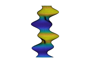
Unlike the single-component system that showed only pearling beyond a particular membrane tension (Boedec et al. Reference Boedec, Jaeger and Leonetti2014; Narsimhan et al. Reference Narsimhan, Spann and Shaqfeh2015), multicomponent vesicles can exhibit richer dynamics. The existence of phase separation, line tension and bending rigidity inhomogeneities can give rise to a combination of pearling, buckling or wrinkling modes at zero or positive membrane tension. We visualize the shape of some of these modes in figure 6. The blue colour indicates the cholesterol-rich ordered $L_{o}$ phase whereas the yellow phase indicates the cholesterol-less disordered $L_{d}$ phase.

Figure 6. Different unstable modes for multicomponent vesicle: (a) pearling $(n=0)$; (b) buckling $(n=1)$; (c) wrinkling $(n=2)$ and (d) wrinkling $(n=3)$.

In the following subsections, we will explore these instabilities in greater detail. We will choose the following parameters in our simulations. We will examine equiviscous vesicles $(\lambda = 1$) as experiments typically inspect this value (Yanagisawa et al. Reference Yanagisawa, Imai and Taniguchi2010). Unless otherwise noted, we will choose a bending difference parameter $\beta = (\kappa _{lo} - \kappa _{ld})/(\kappa _{l0} + \kappa _{ld}) = 0.5$, since we find that $\beta$ in the range listed in table 2 does not qualitatively alter results. We will also choose the Péclet number $1 \leq Pe \leq 100$ consistent with experimental studies (Negishi et al. Reference Negishi, Seto, Hase and Yoshikawa2008; Luo & Maibaum Reference Luo and Maibaum2020).

The structure of the remaining sections are as follows. Section 5.2 characterizes which modes are the most dominant and provides a discussion when multimodal instabilities can be present. Section 5.3 quantifies the most unstable wavenumbers. Section 5.4 discusses the role of Péclet number on the instability, while § 5.5 discusses the role of surface viscosity and provides an analytic expression for when instability occurs. Section 5.6 performs an energy analysis to understand the mechanism of these instabilities. Lastly, we make a side note for the special case of $Pe \ll 1$, where analytical solutions to the eigenvalues and eigenvectors are available. While we believe this case is not physically relevant (see table 2), § A.4 provides details of this analysis for those who are interested.

5.2. Which modes are most dominant?

Here, we delineate the conditions under which the axisymmetric $(n=0)$ instability has the largest growth rate, and the conditions under which the non-axisymmetric instabilities ($n \geq 1$) have the largest growth rate. We will examine the $n = 0,1,2,3$ modes here since we find that $n > 3$ does not dominate for the parameter ranges simulated. When calculating the most dangerous mode, we explore the wavenumber range $0 < k < 3$.

Figure 7 plots which mode has the largest growth rate for different values of the non-dimensional surface tension $(\varGamma )$, Cahn number ($Cn$) and line tension parameter ($\alpha$). Figure 7(a) shows results for a highly compressed vesicle ($\varGamma = -4$), figure 7(b) for a moderately compressed vesicle ($\varGamma = -2$), figure 7(c) for a vesicle under no tension $({\varGamma = 0})$ and figure 7(d) for a vesicle under strong tension $(\varGamma = 30)$. Under strong compression ($\varGamma = -4$, figure 7a), we see that only the non-axisymmetric modes are dominant $(n \neq 0)$. This observation is similar to what is seen for single-component vesicles, although we note that for this value of tension $\varGamma = -4$, only the $n = 1$ and $n = 2$ modes are unstable for the single-component case, while $n=2$ and $n=3$ mostly dominate for the multicomponent case. For very small values of the Cahn number (sharp interface), the dominant modes become more non-axisymmetric, a trend that is seen in all four plots here.

Figure 7. Phase plots for the most dominant mode. The black circles represent the case where $n=0$ dominates, the blue squares where $n=1$ dominates, the red diamonds where $n=2$ dominates and the green diamonds where $n=3$ dominates. The simulation parameters are $\lambda = 1, Pe = 1, \beta = 0.5, {Bq=0}$.

When the vesicle is under moderate compression ($\varGamma = -2$, figure 7b) or no compression ($\varGamma = 0$, figure 7c), all modes $n = 0, 1, 2, 3$ can be unstable depending on the value of Cahn number $(Cn)$ and line tension parameter $(\alpha$). These results are very different than what is seen for single-component vesicles where no modes are unstable at zero tension ($\varGamma = 0$) and only the $n=1$ mode is unstable at moderate compression ($\varGamma = -2$). It also appears that $\alpha$ plays a more significant role in the mode selection than the highly compressed vesicle case ($\varGamma = -4$, figure 7a).

When the vesicle is under large tension ($\varGamma = 30$, figure 7d), the phase plot looks similar to the zero-tension case, except that a larger portion of the phase space shows axisymmetric modes ($n = 0$) being dominant. When the tension becomes very large $(\varGamma \rightarrow \infty )$, one will only observe pearling modes, recovering the results from the single-component case.

We note that while this analysis shows phase plots for the most unstable modes, it does not comment on the magnitude of these growth rates compared with other modes. Below, we will see that in many situations, the growth rates of different modes can be comparable. When this is the case, mode mixing can arise in nonlinear simulations (discussed in § 6).

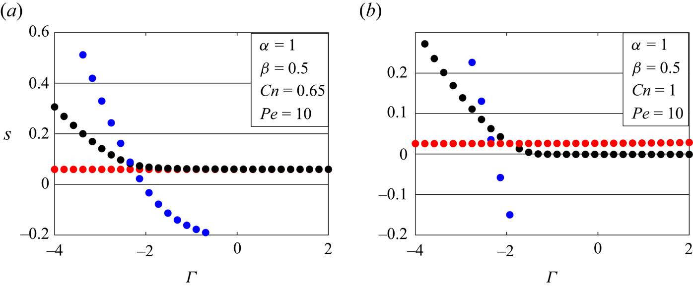
Figure 8 presents the magnitude of the most unstable growth rates for the three modes $n=0,1,2$ with respect to the isotropic membrane tension $\varGamma$. The dimensionless parameters $\lambda = 1$, $\alpha = 1$, $\beta = 0.5$ and $Pe=10$ are chosen to be representative of the experimental values of Yanagisawa et al. (Reference Yanagisawa, Imai and Taniguchi2010) (see § 6.2 for more details). Based on the interface width between the ordered and disordered phases, we could have different values of the Cahn number. We pick two values here: $Cn=0.65,1$. We observe that for lower Cahn numbers $(Cn = 0.65)$, the buckling and wrinkling modes dominate over pearling modes at compressive values of membrane tension. As the tension increases, the growth rates become comparable for pearling and buckling. As the Cahn number increases to 1 (figure 8b), the wrinkling and buckling modes dominate for highly compressive tensions ($\varGamma <-2$), but become stabilized for small compressive and positive values of $\varGamma$, where the pearling modes become dominant. This leads to pure pearling instabilities that will be discussed in detail in § 6.2.

Figure 8. Most unstable growth rates with respect to the isotropic membrane tension $\varGamma$ for multicomponent vesicles. The red circles represent $n=0$ pearling modes, black circles represent $n=1$ buckling modes and blue circles represent $n=2$ wrinkling modes. The dimensionless parameters are (a) $\lambda =1, Pe=10, \alpha = 1, {\beta = 0.5}, Cn =0.65,Bq=0$ and (b) $\lambda =1, Pe=10, \alpha = 1, \beta = 0.5, Cn =1, {Bq=0}$.

5.3. Wavenumber dependence of growth rates

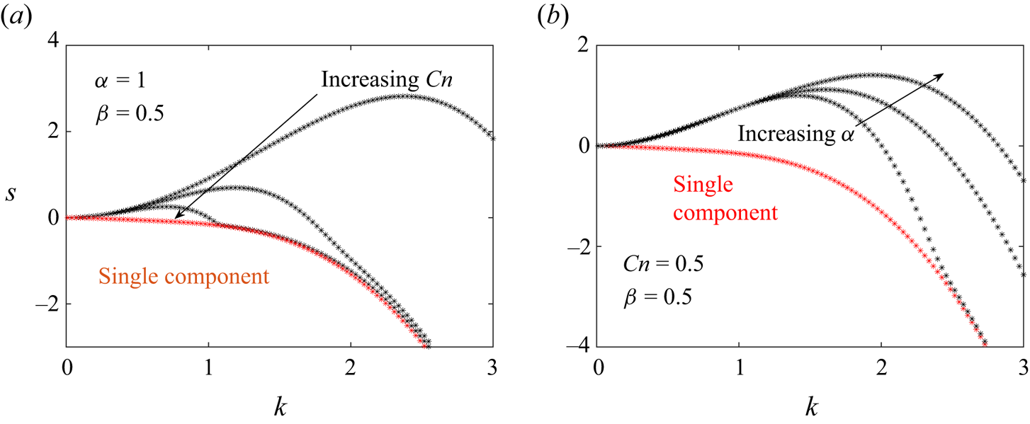
Figures 9–11 plot the wavenumber dependence of the growth rates for different instabilities – the pearling mode ($n = 0$, figure 9), buckling mode ($n = 1$, figure 10) and wrinkling mode ($n=2$, figure 11). In these plots, the membrane tension is $\varGamma =0$. Generally, we observe the following trends: as the Cahn number $Cn$ increases and the line tension parameter $\alpha$ decreases, the maximum growth rate decreases and the most dangerous wavenumber decreases (i.e. the wavenumber $k$ corresponding to the maximum growth rate). These trends occur because large $Cn$ and small $\alpha$ values correspond to large line tensions, which suppresses growth rates and disfavours short wavelength (i.e. large $k$) instabilities. We note that the extent to which the growth rates are altered depends greatly on the mode number ($n$) – this is why for certain values of ($\alpha, Cn$), the pearling modes have the largest growth rate, but for other values, the non-axisymmetric modes have the largest growth rate. We also see that while large $Cn$ and small $\alpha$ values suppress short wavelength (i.e. $k > 1$) instabilities, $Cn$ plays a more significant role in altering the low wavenumber ($k < 1$) growth rates compared with $\alpha$.

Figure 9. Growth rate ($s$) versus wavenumber ($k$) for pearling ($n = 0$) mode. (a) Dependence on Cahn number ($Cn=0.3,0.6,1$) for $\alpha =1, \beta = 0.5, Pe = 1$. (b) Dependence on line tension parameter ($\alpha =0.1,10,20$) for $Cn = 0.5, \beta = 0.5, Pe = 1$. In both graphs, the multicomponent (black) results are compared against single-component (red) results for $\varGamma = 0, \lambda = 1, {Bq=0}$. (a) Variation with $Cn$ and (b) variation with $\alpha$.

Figure 10. Growth rate ($s$) versus wavenumber ($k$) for buckling $(n = 1)$ mode. (a) Dependence on Cahn number ($Cn=0.3,0.6,1$) for $\alpha =1, \beta = 0.5, Pe = 1,{Bq=0}$. (b) Dependence on line tension parameter ($\alpha =0.1,10,20$) for $Cn = 0.5, \beta = 0.5, Pe = 1,{Bq=0}$. In both graphs, the multicomponent (black) results are compared against single-component (red) results for $\varGamma = 0, \lambda = 1$. (a) Variation with $Cn$ and (b) variation with $\alpha$.

Figure 11. Growth rate ($s$) versus wavenumber ($k$) for wrinkling ($n = 2$) mode. (a) Dependence on Cahn number ($Cn=0.2, 0.3, 0.6$) for $\alpha = 1, \beta = 0.5, Pe = 1, {Bq=0}$. (b) Dependence on line tension parameter ($\alpha =0.1, 10, 20$) for $Cn = 0.2, \beta = 0.5, Pe = 1,{Bq=0}$. In both graphs, the multicomponent (black) results are compared against single-component (red) results for $\varGamma = 0, \lambda = 1$. (a) Variation with $Cn$ and (b) variation with $\alpha$.

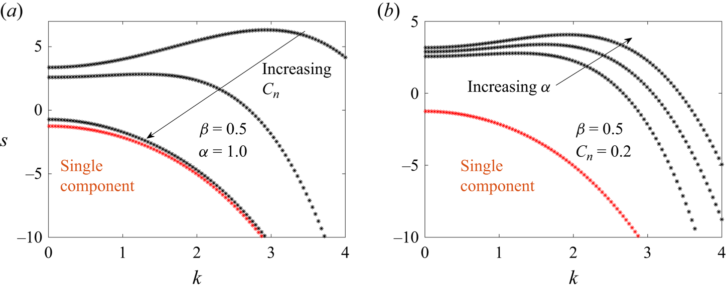
Some of our trends seem consistent with previous simulations of non-tubular vesicles (Gera Reference Gera2017). Specifically, the cited study found that increasing $\alpha$ forms shorter wavelength (larger $k$) stripes on the vesicle, consistent with our study. However, Gera finds that as $\alpha$ rises, it appears that the time slows down to reach the observed behaviour, which is opposite of the growth rate trends observed here (see figures 9b–11b). We point the reader to several caveats: first, the study by Gera inspects non-tubular vesicles, which is different than the geometry considered here. Second, the study examines the full nonlinear dynamics, whereas this section inspects the linearized dynamics and hence the onset of instabilities. Section 6 will provide some results for a weakly nonlinear analysis and compare the results to the linear theory.

Lastly, we inspect the variation of the most unstable wavenumber with respect to the membrane tension $\varGamma$ for different modes $n=0,1,2$ at the experimentally realizable ranges of parameters. Since this variation is not large, we have added these plots to the Appendix (see § A.5).

5.4. Effect of Péclet number on instability

In figure 12, we explore the effect of $Pe$ on the growth rates of instabilities. From (3.18), we can see that the $Pe$ does not alter the onset of instability (determined by the right-hand side of that equation). However, it heavily influences the growth rate of the most unstable mode. We choose a particular set of values $\alpha =1,Cn=0.65, Bq=1,\varGamma =2,\lambda =1$ and vary the $Pe$ over a wide range since it is governed by the average bending stiffness $(k_{0})$, viscosity $(\mu )$, mobility of phospholipids $(\nu )$ and the size $(R)$. From previous experiments (Yanagisawa et al. Reference Yanagisawa, Imai and Taniguchi2010), we see that $R\sim O(1{-}10)\ \mathrm {\mu }$m. This sets the $Pe\sim O(10{-}100), Cn\sim O(0.1{-}1),\alpha \sim O(1)$. At experimentally relevant conditions, as discussed in § 6.2, $Pe\sim O(100)$ and the bending time scale is $t_{b} = \mu R^{3}/k_{0} \sim 0.01$ s, which implies that the coarsening time scale $t_{coarsen} = R^{2}/\nu \sim 1$ s. At these $Pe$ values, the coarsening dynamics decides the magnitude of growth rate, which gives rise to the $s_{max} \sim Pe^{-1}$ scaling in figure 12.

Figure 12. Dependence of the most unstable growth rate on Péclet number $Pe={k_{0}}/{\nu \mu R}$. The other values are $\alpha =1,\beta = 0.5, Cn=0.65,Bq=1,\varGamma =2,\lambda =1$.

5.5. Effect of surface viscosity and general condition for instability

Surface viscosity is a fundamental parameter that affects dynamics of vesicles significantly. One study is worth mentioning here since it pertains to the effect of surface viscosity on the dynamics of vesicles and curved surfaces (Ambruş et al. Reference Ambruş, Busuioc, Wagner, Paillusson and Kusumaatmaja2019). The authors considered inertial dynamics driven by convective coarsening in the system.

To understand the effect of $Bq$, we did the following. For a given value of planar wavenumber $n$ ($n = 0,1$), we found the most dangerous wavenumber $k_{max}$ that yields the largest growth rate. For this wavenumber $k_{max}$, there are two eigenvalues and eigenvectors associated with the $2 \times 2$ linear system in (3.18) – one that corresponds to the most dangerous mode ($\lambda _1$) and another that is subdominant ($\lambda _2$). We plot the eigenvalues ($\lambda _{1},\lambda _{2}$) corresponding to $n=0$ and $n=1$ in figures 13 and 14, respectively. The main observation that can be made is that $\lambda _{2}$ is largely suppressed as $Bq$ increases, whereas the most dangerous mode $\lambda _1$ is largely unaffected. The behaviour of the subdominant eigenvalue $\lambda _2$ is similar to the behaviour seen in single-component vesicles. We believe the reason for these observations is the following: the eigenvector $[r_{kn},q_{kn}]$ corresponding to $\lambda _2$ tends to have a larger component in the shape ($r_{kn}$) direction compared with the concentration ($q_{kn}$) direction. The Boussinesq number $Bq$ primarily affects the shape dynamics $r_{kn}$ as it appears in the term $\varLambda _{kn}$ in (3.18), but plays a smaller role in the $q_{kn}$ dynamics.

Figure 13. Pearling mode ($n=0$) eigenvalues corresponding to (3.18) at the most dangerous wavevector $k_{max}$. The parameters are $\alpha =1,\beta =0.5,Pe=0.1,Cn=0.65,a=-1,b=1$. We choose $Bq=0.1,1,1000$.

Figure 14. Buckling mode ($n=1$) eigenvalues corresponding to (3.18) at the most dangerous wavevector $k_{max}$. The parameters are $\alpha =1,\beta =0.5,Pe=0.1,Cn=0.65,a=-1,b=1$. We choose $Bq=0.1,1,1000$.

A limit often relevant in the case of two-dimensional (2-D) hydrodynamics corresponds to $Bq\to \infty$. This case has been explored by Bachini et al. (Reference Bachini, Krause, Nitschke and Voigt2023b), where they considered the Saffman–Delbruck length to be $l_{SD} \rightarrow \infty$. In this limit, we expect that the dynamics would be governed by the mixing terms $M_{kn},V_{kn}$ in (3.17). This would be very similar to the surface Cahn–Hilliard equation on curved surfaces as explored by the authors.

To conclude this discussion, we leave the reader with a more general condition for stability. From (3.18), we can evaluate the condition for instability to be

(5.1)\begin{equation} \text{det}\begin{bmatrix} L_{kn} & M_{kn} \\ M_{kn} & V_{kn} \\ \end{bmatrix}<0. \end{equation}

This gives us

(5.2)\begin{align} &\left[\varGamma(n^{2}+k^{2}-1) + \frac{3}{2}+2k^{2} +(n^{2}+k^{2})\left(n^{2}+k^{2}-\frac{5}{2}\right)\right] [\tilde{a}+Cn^{2}(n^{2}+k^{2})] \nonumber\\ &\quad <\alpha\beta Cn^{2}(n^{2}+k^{2}-1)^{2}. \end{align}

Based on the choice of $\tilde {a}, Cn,\varGamma,\alpha,\beta$, we can generate the set of unstable pairs of $n,k$. Note that from the above analysis, there are situations where a vesicle that would otherwise be stable in the absence of coupling (i.e. $\beta = 0$, $L_{kn}, V_{kn} > 0$) is unstable when coupling is present ($\beta \neq 0$). Figure 22 in § A.6 gives an example of this situation.

5.6. Energy analysis

There are three energetic contributions to the instability: bending energy, phase energy and surface tension energy (see § 2.1). To understand which contributions play the largest role, we perform the following analysis. We take the base state of the cylindrical vesicle ($r_0 = 1, q_0 = 0$), and perturb the radius and concentration as follows:

(5.3)$$\begin{gather} r = 1 + \epsilon r_{kn} \cos{(kz+n\phi)} - \tfrac{1}{4}\epsilon^{2} r_{kn}^2, \end{gather}$$

(5.4)$$\begin{gather}q = \epsilon q_{kn} \cos{(kz+n\phi)} - \tfrac{1}{2} \epsilon^2 q_{kn} r_{kn}. \end{gather}$$

The higher order terms are present to conserve the volume and order parameter to $O(\epsilon ^2)$: i.e. $V = V_0$ and $\int q dS = 0$. We then compute the change in energy between the perturbed and base states, and break them into the bending ($b$), phase ($p$) and surface tension ($\sigma$) contributions:

(5.5)\begin{align} \Delta E &= E(r_{kn}, q_{kn}) -{-} E(r_{kn} = 0, q_{kn} = 0) \end{align}

(5.6)\begin{align} &= \Delta E_b + \Delta E_p + \Delta E_{\sigma}. \end{align}

If $\Delta E < 0$, the perturbation has a lower energy than the base state, which leads to instability. If $\Delta E > 0$, the perturbation has a higher energy than the base state, and thus the base state is locally stable. Below are the bending, phase and surface tension contributions to the energy change per unit length of the vesicle. The algebraic details are given in § A.7.

(5.7)\begin{gather} \Delta E_b = \frac{{\rm \pi} \epsilon^2 {r_{kn}}^2}{2}\left(2k^{2} +{(k^{2}+n^{2})\left(k^{2}+n^{2}-\frac{5}{2}\right) + \frac{3}{2}}\right) \nonumber\\ \quad + \beta {\rm \pi}\epsilon^{2} r_{kn} q_{kn} (k^{2}+n^{2}-1), \end{gather}

(5.8)$$\begin{gather} \Delta E_p = \frac{{\rm \pi} \epsilon^2 q_{kn}^2}{2 \alpha Cn^2}[\tilde{a} + Cn^2 (n^2 + k^2)], \end{gather}$$

(5.9)$$\begin{gather}\Delta E_{\sigma} = \frac{\varGamma{\rm \pi}\epsilon^2 r_{kn}^2}{2}(n^2 + k^2 -1). \end{gather}$$

In figure 15, we examine the energetic contributions to the pearling $(n = 0)$ mode at $\lambda =1,Pe=3,\alpha =1$. Here, we use the linear stability theory to compute the dominant eigenvector $[r_{kn}, q_{kn}]$ at the most unstable wavenumber $k$, and then compute the energetic contributions ($\Delta E_b, \Delta E_p, \Delta E_{\sigma }$) as stated above for perturbation value $\epsilon = 0.1$. We vary the value of $Cn$ while keeping $\varGamma$ fixed at $-4$ and $5$, both representing extremes of compression and tension, respectively. It can be seen that for experimentally relevant values of the Cahn number $Cn$, the phase energy is the primary driver for the destabilization of the vesicle shape for highly compressive values of $\varGamma$ (figure 15a). The bending energy seems to have a stabilizing effect on the vesicle pearling whereas the tension has a weakly destabilizing effect. When the value of $\varGamma$ is largely positive, as the $Cn$ increases, the tension energy begins destabilizing the vesicle more than the phase energy whereas the bending energy is always stabilizing (figure 15b).

Figure 15. Energetic contributions to the pearling mode ($n=0$) for different values of $Cn$ and $\varGamma$. The red circles represent phase energy ($\Delta E_p$), blue circles represent the bending energy ($\Delta E_b$) and the black circles represent the surface tension energy ($\Delta E_{\sigma }$). The parameters are $\lambda = 1, Pe = 3, \alpha = 1,\epsilon =0.1,{Bq=0}$. (a) $\varGamma =-4$ and (b) $\varGamma =5$.

In figure 16, we examine the energetic contributions to the buckling $(n = 1)$ mode at $\lambda =1,Pe=3,\alpha =1$. We vary the value of $Cn$ while keeping $\varGamma$ fixed at $-4$ and $5$, both representing extremes of compression and tension, respectively. It can be seen that for experimentally relevant values of the Cahn number $Cn$, for highly compressive values of $\varGamma$, the tension energy causes the largest destabilization of the vesicle shape as the $Cn$ increases whereas the phase energy contributes less (figure 16a). The bending energy seems to have a stabilizing effect on the buckling. When the value of $\varGamma$ is largely positive (figure 16b), we see that the phase energy is the primary driver for the destabilization of the vesicle shape.

Figure 16. Energetic contributions to the buckling mode ($n=1$) for different values of $Cn$ and $\varGamma$. The red circles represent phase energy ($\Delta E_p$), blue circles represent the bending energy ($\Delta E_b$) and the black circles represent the surface tension energy ($\Delta E_{\sigma }$). The parameters are $\lambda = 1, Pe = 3,{Bq=0}, \alpha = 1,\epsilon =0.1$. (a) $\varGamma =-4$ and (b) $\varGamma =5$.

6.1. Solving nonlinear equations

We perform a weakly nonlinear stability analysis on the base state mentioned in § 3.1. We perturb all geometric and physical quantities an infinitesimal amount $\epsilon \ll 1$ as shown below:

(6.1a)$$\begin{gather} r = 1 + \epsilon \sum_{kn}{r_{kn}\exp({\rm i}kz+{\rm i}n\phi)}, \end{gather}$$

(6.1b)$$\begin{gather}\sigma = \varGamma + \epsilon \sum_{kn}{\sigma_{kn}\exp({\rm i}kz+{\rm i}n\phi)}, \end{gather}$$

(6.1c)$$\begin{gather} \boldsymbol{u}^{in/out} =\epsilon\sum_{kn}{\boldsymbol{u}_{kn}^{in/out} \exp({\rm i}kz+{\rm i}n\phi)}, \end{gather}$$

(6.1d)$$\begin{gather}q = \epsilon \sum_{kn}{q_{kn}\exp({\rm i}kz+{\rm i}n\phi)}, \end{gather}$$

(6.1e)$$\begin{gather}p^{in} = \varGamma - \frac{1}{2} + \epsilon \sum_{kn}{p_{kn}^{in}\exp({\rm i}kz+{\rm i}n\phi)}, \end{gather}$$

(6.1f)$$\begin{gather}p^{out} = \epsilon \sum_{kn}{p_{kn}^{out}\exp({\rm i}kz+{\rm i}n\phi)}. \end{gather}$$

To understand the coarsening dynamics more quantitatively, we solve the linearized shape equation ((3.17)) along with the Cahn–Hilliard equation given by

(6.2)\begin{align} \frac{{\rm d}q_{kn}}{{\rm d}t} &={-}\frac{\mathscr{F}(\boldsymbol{u}\boldsymbol{\cdot}\boldsymbol{\nabla}_{s}q)}{Pe} -\frac{(n^{2}+k^2)}{Pe}[\tilde{a}+Cn^{2}(n^2+k^2)]q_{kn} -\frac{\tilde{b}(n^{2}+k^{2})}{Pe}\mathscr{F}(q^{3})\nonumber\\ &\quad -\alpha\beta Cn^{2}(n^{2}+k^{2})(n^{2}+k^{2}-1)r_{kn}. \end{align}

The equation above is the same as (3.2), except that two nonlinearities are added: a convective term $-{\mathscr {F}(\boldsymbol {u}\boldsymbol {\cdot }\boldsymbol {\nabla }_{s}q)}/{Pe}$ and the chemical potential from the quartic portion of the free energy $-({\tilde {b}(n^{2}+k^{2})}/{Pe})\mathscr {F}(q^{3})$, where $\mathscr {F}(\cdots )$ represents a Fourier transform. Keeping the entire quartic potential in the Cahn–Hilliard equation allows the concentration and shape fields to evolve to an equilibrium state. We emphasize that we solve the full Cahn–Hilliard equations in the small deformation limit by retaining the nonlinear convective and quartic potential terms. The numerical procedure is mentioned in § A.8.

In figure 17, we perform a one-to-one comparison of linear and nonlinear simulations from the same initial condition, to understand when these two simulations start deviating from each other. In this figure, based on the parameters mentioned in the caption, the linear stability analysis predicts most unstable growth rates to be $s_{max}=0.04152$ for $n=0$, $s_{max}=0.04237$ for $n=1$, $s_{max}=0.02977$ for $n=2$. According to these values, at early times, there should be a mix of buckling, pearling and wrinkling, whereas at longer times, buckling should dominate with some pearling effects. The corresponding nonlinear simulations predict similar dynamics up to $t\sim 250$, which can translate to 12–25 s, beyond which we see buckling dominating with spiral order parameter patterns due to mode-mixing. The time window of matching between the linear and nonlinear dynamics is experimentally relevant and depends heavily on the $Pe$ value. As discussed previously, for higher $Pe$ values, the linear growth rates reduce in magnitude thereby delaying the nonlinear effects. For larger $Cn$ values, the dynamics become comparable over an even longer time window. This comparison is done in figure 18 where we can see that the patterns look similar up to $t\sim 1000$, which corresponds to $t\sim 50{-}100$ s. This is an example of the linear theory working well at experimental time scales. Generally, linear and nonlinear dynamics show qualitatively similar shapes and concentration profiles at long times when only one mode is considered to be dominant (e.g. figure 18 where only pearling is the dominant mode for $Cn \geq 0.8$ with the other parameters kept the same as figure 17).

Figure 17. Linear versus nonlinear simulations for $\alpha =1,\beta =0.5,\varGamma =2,a=-1,b=1,Cn=0.45, Pe=30,Bq=1$. The initial condition is $r=1, q=\epsilon (2\times rand-1)$ on a $32\times 32$ grid where $z \in [-10,10]$, $\phi \in [0,2{\rm \pi} ]$, with both simulations using the same seed in random number generation. The time step size is $\Delta t = 0.01$ and $\epsilon = 0.001$. The colourbar represents the value of ${q}/{|q|}$. The nonlinear simulation video (figure 17a) is given in Movie 4 of the supplementary movies at https://doi.org/10.1017/jfm.2024.1120.

Figure 18. Linear versus nonlinear simulations for $\alpha =1,\beta =0.5,\varGamma =2,a=-1,b=1,Cn=0.8, Pe=30,Bq=1$. The initial condition is $r=1, q=\epsilon (2\times rand-1)$ on a $32\times 32$ grid where $z \in [-10,10]$, $\phi \in [0,2{\rm \pi} ]$, with both simulations using the same seed in random number generation. The time step size is $\Delta t = 0.01$ and $\epsilon = 0.001$. The colourbar represents the value ${q}/{|q|}$. The nonlinear simulation video (figure 18a) is given in Movie 3 of the supplementary movies.

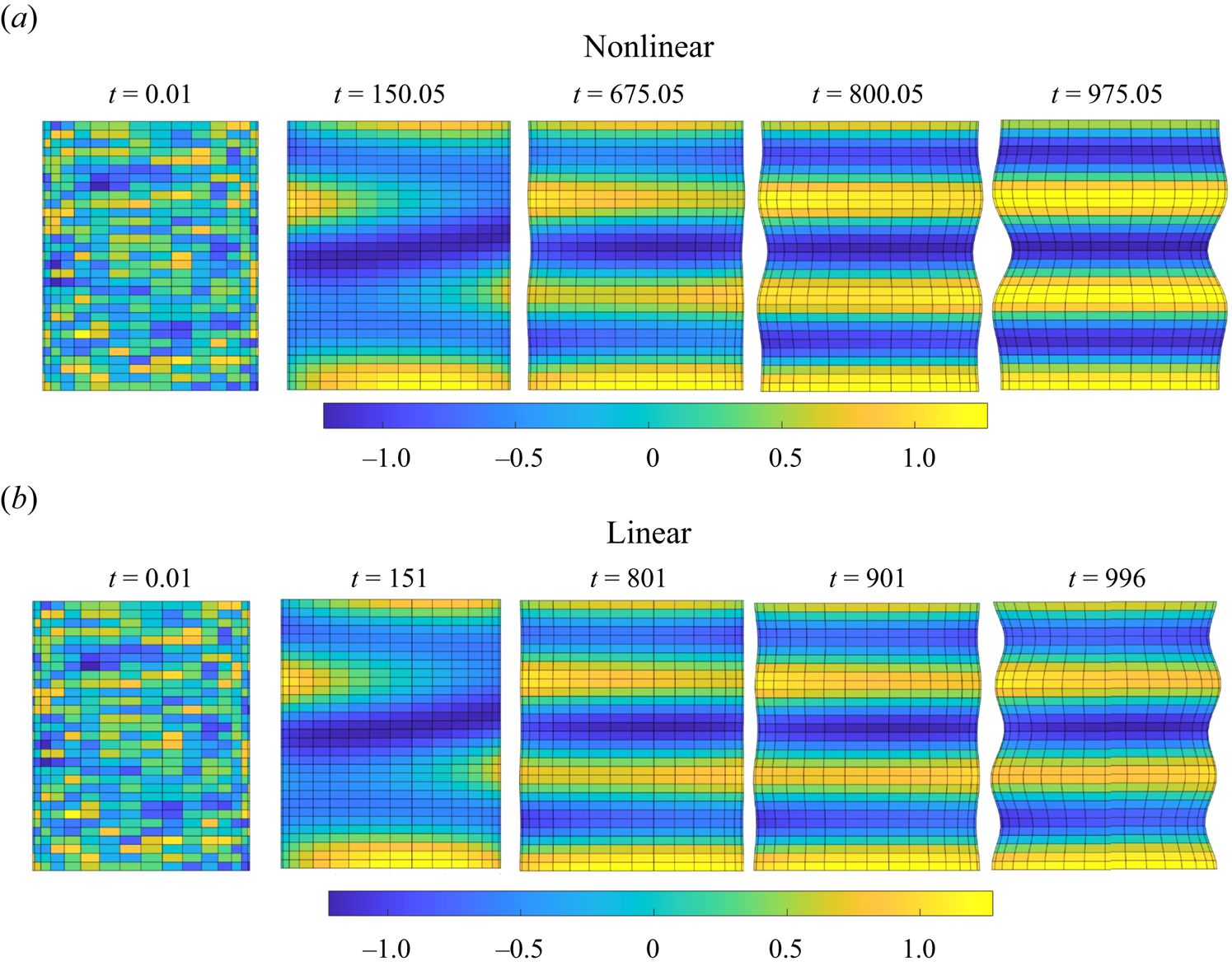
6.2. Experimental comparison

In this section, we compare our nonlinear dynamical simulations with experimental observations from (Yanagisawa et al. Reference Yanagisawa, Imai and Taniguchi2010). In this paper, the authors explored periodic modulations in cylindrical, multicomponent vesicles containing DOPC/DPPC/cholesterol at 1 : 1 DOPC : : DPPC and different amounts of cholesterol. The vesicles were created by taking spherical giant unilamellar vesicles (GUVs) with these lipids, and osmotically deflating them to create tubular shapes of radius $R \approx 0.5{-}3\ \mathrm {\mu }$m with aspect ratios between $L = 5\textrm { and }20$. The modulations observed arose due to the phase separation into liquid-ordered $(L_o)$ and liquid-disordered $(L_d)$ phases, similar to what is seen in our theories. The interior and exterior fluids were the same (up to the sugars used for osmotic deflation), yielding a viscosity ratio $\lambda \approx 1$. Based on the ratios of DOPC : DPPC : Chol in their studies, the average bending stiffness was estimated to be $k_0 \approx 10^{-19}\ \textrm {J}$ and the difference in bending stiffness between domains varied in the range $\beta = 0.1{-}0.5$. The line tension was estimated to be roughly $1$ pN, yielding a line tension parameter $\alpha \approx 1$. Examining the interface width yields a Cahn number $Cn = \varepsilon ^{width}/(\sqrt {2}R) \approx 0.3{-}1$. We find that results are highly sensitive to this parameter as shown below. The Péclet number was estimated to be $Pe = O(10){-}O(100)$ based on limited data of lipid diffusivities (Negishi et al. Reference Negishi, Seto, Hase and Yoshikawa2008).

The only non-dimensional number we were not able to infer from experimental data was the dimensionless surface tension $\varGamma = \sigma _0 R^2/k_0$, since the surface tension $\sigma _0$ was not provided. In principle, one could obtain $\sigma _0$ by performing an equilibrium simulation of vesicle shape since this quantity arises as a Lagrange multiplier that enforces the constant area of the membrane. However, this simulation is quite difficult to do for highly deflated, multicomponent vesicles (and to our knowledge has yet to be performed). Instead, we make a note that $\sigma _0$ is likely to be very small since the vesicles are under no external force, and for values $\sigma _0 = 10^{-7}\ \textrm {N}\ \textrm {m}^{-1}$, this yields $\varGamma \sim O(1)$. Thus, we will perform simulations for several different values of $\varGamma$ and see how they compare against experimental data. We will also vary $Cn$ since the results are sensitive to this value. For the other parameters, we set $\lambda = 1, Pe =10, \alpha = 1, \beta = 0.5,{Bq=1}$ consistent with estimated values listed above. The characteristic time scale using the parameters chosen above corresponds to the bending scale $t_{b}=\eta R^{3}/k_{0} \approx 0.01$ s. In the following results (figures 19 and 20), we simulate the dynamics up to $t \sim 1000$ bending times, which would correspond to ${\sim }10$ s. From the experimental paper in discussion (Yanagisawa et al. Reference Yanagisawa, Imai and Taniguchi2010), the dynamics are observed over ${\sim }45$ s. This seems comparable but not exactly accurate. We note that the choice of $Pe$ plays a very important role here. We have assumed the lipid diffusivity to be $\nu = 10^{-11}\ \textrm {m}^2\ \textrm {s}^{-1}$, but there have been recent studies that have shown this value to be potentially even lower $O(10^{-12}\ \textrm {m}^2\ \textrm {s}^{-1})$ (Pöhnl, Trollmann & Böckmann Reference Pöhnl, Trollmann and Böckmann2023). In these cases, the $Pe$ could go to $100$ for the same set of experimental parameters chosen by us. If this happens, the dynamics would be governed by the coarsening time scale and not the bending time scale. This would reduce the growth rate of our instabilities and could cause the simulation time scale to be comparable to the experimental time scale.

Figure 19. Pearling visual qualitative comparison with experiments (Yanagisawa et al. Reference Yanagisawa, Imai and Taniguchi2010) where the yellow domains represent the cholesterol rich $L_{o}$ phase (black in experiments) and the blue domains (white in experiments) represent the cholesterol-lacking $L_{d}$ phase. The parameters for the simulation are $\lambda = 1, Pe =10, \alpha = 1, \beta = 0.5,{Bq=1}, Cn =0.8,$ and $\varGamma = 0$ corresponding to a vesicle radius $R\approx 1\ \mathrm {\mu }$m. The system is simulated up to time $t = 1000$, which translates to a physical time of $10$ s. The initial condition is $q=\epsilon ( 2*\textrm {rand} - 1)$ on a $64\times 64$ grid with $z \in [-10,10]$, $\phi \in [0,2{\rm \pi} ]$, where $\epsilon = 0.01$. The scale bar represents a length of $5\ \mathrm {\mu }$m. The mole fraction ratio of DOPC : DPPC : Chol is 9 : 9 : 22. The colourbar represents the value of ${q}/{|q|}$. The nonlinear simulation video is given in Movie 2 of supplementary movies. Experimental image is reproduced with permission from Yanagisawa et al. (Reference Yanagisawa, Imai and Taniguchi2010).

Figure 20. Mixed mode instability found in experiments (Yanagisawa et al. Reference Yanagisawa, Imai and Taniguchi2010) and simulations. The pearling mode $(n = 0)$ can have a larger wavenumber compared with the buckling mode $({n = 1})$. The parameters for the simulation are $\lambda = 1, Pe = 10, \alpha = 1,{Bq=1}, \beta = 0.5, Cn=0.3$ and $\varGamma =2$ corresponding to $R=1\ \mathrm {\mu }$m. The system is simulated up to time $t = 1000$, which translates to a physical time of $10$ s. The initial condition is $q=\epsilon ( 2*\textrm {rand} - 1)$ on a $32\times 32$ grid where $z \in [-10,10]$, $\phi \in [0,2{\rm \pi} ]$, where $\epsilon = 0.01$. The inset scale bar represents a length of $2\ {\rm \mu}$m. The mole fraction ratio DOPC : DPPC : Chol is 3 : 3 : 4. The colourbar represents the value of ${q}/{|q|} \in [-1,1]$. The nonlinear simulation video is given in Movie 1 of supplementary files. Experimental image is reproduced with permission from Yanagisawa et al. (Reference Yanagisawa, Imai and Taniguchi2010).

In figure 19, we show one snapshot of an experimental image where the vesicle forms a straight line with pearls. The bright regions represent the disordered $L_{d}$ phase and the dark regions represent the ordered $L_{o}$ phase. The interface width is fairly diffuse, leading to $Cn \approx 0.8$. If we perform nonlinear simulations with no tension $\varGamma = 0$, we observe qualitatively similar behaviour to experiments. These snapshots are shown at various time steps, with similar behaviour also seen for $\varGamma >0$ (not shown). For the simulated case, the linear stability analysis also predicts pearling shapes like the nonlinear analysis, albeit with a more aggressive growth rate ($s = 0.039$ for linear result, corresponding to time scale $t = 1/s \approx 25$ as opposed to $t \sim O(100)$ for nonlinear simulations). However, if $Pe \geq 50$ (which could be realistic based on the uncertainty for lipid diffusivities), the growth rates from the linear analysis could be comparable to the experimentally relevant time scales $t \sim O(100)$ s.

In the experiments, vesicles occasionally exhibited buckling in addition to pearling. In these situations, the interface width appears sharper than the case when pearls form. Figure 20 shows a snapshot of such an example using nonlinear simulations with a sharper interface $Cn = 0.3$ and slightly positive tension $\varGamma = 2$. The nonlinear simulations at intermediate times show pearling and buckling modes (the corresponding linear stability analysis shows that $s=0.1802$ for $n=0$, $s=0.24$ for $n=1$ and $s=0.28$ for $n=2$, thereby showing buckling, wrinkling and pearling), but at long time, the nonlinear analysis shows buckling with a diagonal concentration stripe. The long-wavelength buckling shape appears similar to the experiment, but the short wavelength pearls are not observed. This may be due to the fact that the simulations assume small deformations, which are clearly not followed in experiments. We note that the shape observed in our simulations is sensitive to the initial condition in the simulation. Just like the pearling case, we believe that based on the $Pe$, the linear dynamics could get delayed thereby giving accurate dynamics at experimentally relevant time scales.