


1. Introduction
Measures of divergence between probability distributions are significant due to their applications in reliability, survival analysis, testing of hypotheses, and classification problems. Divergence measures based on entropy and extropy measures are introduced in the literature. Based on Shannon entropy [Reference Shannon15], Kullback and Leibler [Reference Kullback and Leibler4] introduced Kullback–Leibler (KL) divergence, which is the pioneering work on divergence measures in information theory. Following the KL divergence, a considerable number of divergence measures have been put forward by different authors, either due to their theoretical foundations or practical applications. Some of them are Rényi’s divergence [Reference Rényi12], Tsallis’s divergence [Reference Tsallis18], etc.
More recently, extropy has emerged as a complementary dual to entropy, offering a novel perspective on uncertainty quantification. According to Lad et al. [Reference Lad, Sanfilippo and Agro5], the extropy of a nonnegative and absolutely continuous random variable  $X$ with a probability density function (p.d.f.) $f$, is defined by
 \begin{equation}
J(X)=-\frac{1}{2}\int_0^{\infty} f^2(x) dx.
\end{equation}
\begin{equation}
J(X)=-\frac{1}{2}\int_0^{\infty} f^2(x) dx.
\end{equation}  $J(X)$ is always nonpositive because of the negative sign in front of the quadratic term. Lad et al. [Reference Lad, Sanfilippo and Agro5] also introduced the concept of relative extropy (RE), which measures the discrepancy between two probability distributions with p.d.f.’s $f$ and $g$ as
 \begin{equation}
d(\,f,g)=\frac{1}{2}\int_0^\infty \left(\,{f(x)}-{g(x)}\right)^2 dx.
\end{equation}
\begin{equation}
d(\,f,g)=\frac{1}{2}\int_0^\infty \left(\,{f(x)}-{g(x)}\right)^2 dx.
\end{equation} In contrast to entropy-based divergence measures, RE possesses the property of symmetry, implying that  $d(\,f,g)=d(g,f)$. A new measure of inaccuracy based on extropy for record statistics between distributions of the $n$th upper (lower) record value and parent random variable was introduced by Hashempour and Mohammadi [Reference Hashempour and Mohammadi1], which is given in the form,
 \begin{equation}
\xi J(X,Y)=-\frac{1}{2}\int_0^\infty f(x)g(x)dx.
\end{equation}
\begin{equation}
\xi J(X,Y)=-\frac{1}{2}\int_0^\infty f(x)g(x)dx.
\end{equation} It is observed that  $d(\,f,g)= 2\xi J(X,Y)-J(X)-J(Y)$. $ \xi J(X,Y)$ measures the inaccuracy caused by assuming $g$ instead of $f$. The dynamic extropy inaccuracy for residual lifetimes, $X_t = (X - t| X \gt t)$ and $Y_t = (Y - t| Y \gt t)$, defined by Hashempour et al. [Reference Hashempour, Toomaj and Kazemi2] as
 \begin{equation}
\xi J_r(X,Y,t)=-\frac{1}{2}\int_t^\infty \frac{f(x)}{\bar{F}(t)}\frac{g(x)}{\bar{G}(t)}dx,
\end{equation}
\begin{equation}
\xi J_r(X,Y,t)=-\frac{1}{2}\int_t^\infty \frac{f(x)}{\bar{F}(t)}\frac{g(x)}{\bar{G}(t)}dx,
\end{equation}equals  $J_t(X) = - \frac{1}{2}\int_{t}^{\infty}{\left(\frac{f(x)}{\bar{F}(t)}\right)^2 dx}$, the dynamic residual extropy when $f(x)=g(x)$. Let $X_{(t)} = (t - X | X \leq t)$ and $Y_{(t)} = (t - Y | Y \leq t)$ be two past lifetime random variables, then the dynamic past inaccuracy measure defined by Mohammadi et al. [Reference Mohammadi, Hashempour and Kamari8] is given as
 \begin{equation}
\xi J_p(X,Y,t)=-\frac{1}{2}\int_0^t\frac{f(x)g(x)}{F(t)G(t)}dx,
\end{equation}
\begin{equation}
\xi J_p(X,Y,t)=-\frac{1}{2}\int_0^t\frac{f(x)g(x)}{F(t)G(t)}dx,
\end{equation}equals  $J(X_{(t)}) = - \frac{1}{2}\int_{0}^{t}{\left(\frac{f(x)}{F(t)}\right)^2 dx}$, the dynamic past extropy when $f(x)=g(x)$. The discrimination measure based on extropy and inaccuracy between density functions $f(x)$ and $g(x)$ is defined by
 \begin{equation}
J(\,f|g)=\frac{1}{2}\int_0^\infty [\,f(x)-g(x)]\,f(x)dx = \frac{1}{2}E_f[\,f(X)-g(X)],
\end{equation}
\begin{equation}
J(\,f|g)=\frac{1}{2}\int_0^\infty [\,f(x)-g(x)]\,f(x)dx = \frac{1}{2}E_f[\,f(X)-g(X)],
\end{equation}which is the expectation of  $(\,f - g)$ with respect to $f$.
$f$.  $J(\,f|g)$ is a measure of directional divergence between two distributions since it is asymmetric, and $J(\,f|g)$ and $J(g|\,f)$ cannot be equal for all $f$ and $g$.
$g$.
Divergence measures based on extropy and its variants are an emerging area of interest due to their advantages in theory and applications. Saranya and Sunoj [Reference Saranya and Sunoj13] proposed a measure of symmetric divergence based on survival extropy and studied its properties and applications. Recently, Saranya and Sunoj [Reference Saranya and Sunoj14] introduced an inaccuracy and divergence measure based on survival extropy, and obtained their various properties and applications in image classification and reliability analysis. Although the literature includes symmetric and asymmetric information measures based on entropy and extropy, each with distinct advantages and applications, the interconnections between the symmetric and asymmetric measures remain relatively unexplored. Investigating these relationships can provide deeper insight into their properties and lead to significant results in information theory and reliability. Lad et al. [Reference Lad, Sanfilippo and Agro5] introduced the concept of a symmetric divergence measure called RE, and Mohammadi et al. [Reference Mohammadi, Hashempour and Kamari8] defined a directional divergence measure called extropy divergence based on extropy. The interrelationships between these two are not explored. Accordingly, the present study focuses on exploring extropy-based relative information measures through their interrelationships.
The paper is organized as follows. In Section 2, we discuss some properties of RE and extropy divergence. We explore the dynamic extensions of RE, extropy divergence, and extropy inaccuracy for residual and past lifetimes, their properties, and characterizations in Section 3. Section 4 investigates the estimation of RE and simulation studies to validate the performance of the estimator. Section 5 demonstrates the practical applications of the measure in the context of lifetime data analysis and image analysis.
2. RE and extropy divergence
The concept of RE is a foundational contribution as a symmetric divergence measure between two probability distributions based on extropy. In this section, we further study the measure, derive some properties of RE and the relationship with extropy divergence. For two nonnegative continuous random variables  $X$ and $Y$ with p.d.f.’s $f$ and $g$, respectively, we have the relationship between RE, extropy inaccuracy, and extropy as:
 \begin{equation*}
d(\,f,g)=2\xi J(X,Y)-J(Y)-J(X).
\end{equation*}
\begin{equation*}
d(\,f,g)=2\xi J(X,Y)-J(Y)-J(X).
\end{equation*} The RE is always nonnegative and zero if and only if  $f(x)=g(x)$ for every $x$. It is a measure of discrimination between two probability distributions based on their density functions. Note that the measure $d(\,f,g)$ is unnormalized and its value is inherently influenced by the support over which the distributions are defined.
Note that  $E_f$ and $E_g$ denote the expectation over density functions $f$ and $g$, respectively. Let $E_f[h(X)] = \displaystyle \int h(x) f(x)\, dx.$ The expression in (1.2) can be rewritten by splitting it as follows:
 \begin{equation*}
\begin{split}
d(\,f,g)&=\frac{1}{2}\int_0^\infty \left(\,{f(x)}-{g(x)}\right)^2 dx \\
&=\frac{1}{2}\left(\int_0^\infty (\,{f(x)}-{g(x)})\,f(x) dx+ \int_0^\infty ({g(x)}-{f(x)}) g(x) dx\right).
\end{split}
\end{equation*}
\begin{equation*}
\begin{split}
d(\,f,g)&=\frac{1}{2}\int_0^\infty \left(\,{f(x)}-{g(x)}\right)^2 dx \\
&=\frac{1}{2}\left(\int_0^\infty (\,{f(x)}-{g(x)})\,f(x) dx+ \int_0^\infty ({g(x)}-{f(x)}) g(x) dx\right).
\end{split}
\end{equation*}In the following theorem, we express the relationship between RE and extropy divergences.
Theorem 2.1. Let  $X$ and $Y$ be two nonnegative random variables with density functions $f$ and $g$, respectively. Then the RE of $X$ and $Y$ can be expressed as the sum of extropy divergences as follows.
 \begin{equation}
d(\,f,g)=J(\,f|g)+J(g|\,f)=\frac{1}{2}(E_f[\,f(X)-g(X)]+E_g[g(X)-f(X)]),
\end{equation}
\begin{equation}
d(\,f,g)=J(\,f|g)+J(g|\,f)=\frac{1}{2}(E_f[\,f(X)-g(X)]+E_g[g(X)-f(X)]),
\end{equation}where  $J(g|\,f)$ is the extropy divergence from $g$ to $f$ with respect to $g$ given as follows:
 \begin{equation*}
J(g|\,f)=\frac{1}{2}\int_0^\infty [g(x)-f(x)]g(x)dx.
\end{equation*}
\begin{equation*}
J(g|\,f)=\frac{1}{2}\int_0^\infty [g(x)-f(x)]g(x)dx.
\end{equation*}Thus, we can represent the symmetric divergence measure based on extropy as the sum of asymmetric divergences based on extropy of both orders.
Corollary 2.1. The quantities  $J(\,f\,|\,g)$ and $J(g\,|\,f)$ can each be negative, positive, or zero. However, their sum yields RE, which is always nonnegative, which in turn implies
 \begin{equation*}
J(\,f\,|\,g) \;\ge\; -\,J(g\,|\,f).
\end{equation*}
\begin{equation*}
J(\,f\,|\,g) \;\ge\; -\,J(g\,|\,f).
\end{equation*} Kullback [Reference Kullback3] studied the approximation of the KL information of  $f(x)$ and $f(x;\theta+\Delta\theta)$. In the following theorem, we provide a theoretical approximation to the RE of two similar densities, that is, between $f(x,\theta)$ and $f(x,\theta+\Delta\theta)$, as follows:
Theorem 2.2. Let  $X$ be a nonnegative random variable with density function $f$ with parameter $\theta$. Let $f(x,\theta)$ be twice differentiable in $\theta$ and $\int \left(\frac{d}{d\theta} f(x,\theta)\right)^2 dx \lt \infty$ and applying the dominated convergence theorem, we obtain
 \begin{equation}
d(\,f(x,\theta),f(x,\theta+\Delta\theta)) \approx \frac{\Delta\theta^2}{2}\int_0^\infty \left(\frac{d}{d\theta}f(x,\theta)\right)^2dx.
\end{equation}
\begin{equation}
d(\,f(x,\theta),f(x,\theta+\Delta\theta)) \approx \frac{\Delta\theta^2}{2}\int_0^\infty \left(\frac{d}{d\theta}f(x,\theta)\right)^2dx.
\end{equation}Proof. Using the Taylor series expansion, for a fixed  $x$ and a small $\Delta\theta$, we obtain
 \begin{equation}
\begin{split}
f(x,\theta+\Delta\theta)&=f(x,\theta)+f'(x,\theta)\Delta\theta+f''(x,\theta)\frac{(\Delta\theta)^2}{2!}+...\\
f(x,\theta+\Delta\theta)-f(x,\theta)&= f'(x,\theta)\Delta\theta+o{(\Delta\theta)^2}.
\end{split}
\end{equation}
\begin{equation}
\begin{split}
f(x,\theta+\Delta\theta)&=f(x,\theta)+f'(x,\theta)\Delta\theta+f''(x,\theta)\frac{(\Delta\theta)^2}{2!}+...\\
f(x,\theta+\Delta\theta)-f(x,\theta)&= f'(x,\theta)\Delta\theta+o{(\Delta\theta)^2}.
\end{split}
\end{equation} Since higher order terms are significantly small for smaller  $\Delta\theta$, (2.3) reduces to
 \begin{equation*}
(\,f(x,\theta+\Delta\theta)-f(x,\theta))^2\approx (\Delta\theta f'(x,\theta))^2.
\end{equation*}
\begin{equation*}
(\,f(x,\theta+\Delta\theta)-f(x,\theta))^2\approx (\Delta\theta f'(x,\theta))^2.
\end{equation*}Then,
 \begin{equation*}
\frac{1}{2}\int_0^\infty (\,f(x,\theta+\Delta\theta)-f(x,\theta))^2 dx\approx \frac{(\Delta\theta)^2}{2}\int_0^\infty f'(x,\theta)^2 dx.
\end{equation*}
\begin{equation*}
\frac{1}{2}\int_0^\infty (\,f(x,\theta+\Delta\theta)-f(x,\theta))^2 dx\approx \frac{(\Delta\theta)^2}{2}\int_0^\infty f'(x,\theta)^2 dx.
\end{equation*} The approximation in (2.2) reveals an interesting connection between the RE and the Fisher information. For small parameter perturbations  $\Delta\theta$, the quantity
 \begin{equation}
\begin{split}
d(\,f(x,\theta),f(x,\theta+\Delta\theta)) &\approx \frac{\Delta\theta^2}{2}\int_0^\infty \left(\frac{\partial f(x,\theta)}{\partial \theta}\right)^2 dx.\\
\end{split}
\end{equation}
\begin{equation}
\begin{split}
d(\,f(x,\theta),f(x,\theta+\Delta\theta)) &\approx \frac{\Delta\theta^2}{2}\int_0^\infty \left(\frac{\partial f(x,\theta)}{\partial \theta}\right)^2 dx.\\
\end{split}
\end{equation} Since the Fisher information of the density function  $f(x,\theta)$ is expressed as
 \begin{equation}
I_f(\theta)=E_f\left[\frac{\partial}{\partial\theta}\log f(x,\theta)\right]^2=\int_0^\infty \left(\frac{\partial}{\partial\theta} f(x,\theta)\right)^2\times \frac{1}{f(x,\theta)}dx ,
\end{equation}
\begin{equation}
I_f(\theta)=E_f\left[\frac{\partial}{\partial\theta}\log f(x,\theta)\right]^2=\int_0^\infty \left(\frac{\partial}{\partial\theta} f(x,\theta)\right)^2\times \frac{1}{f(x,\theta)}dx ,
\end{equation}we define a weighted Fisher information with weight  $w(x,\theta)=\sqrt{f(x,\theta)}$ as
 \begin{equation}
I_{f}^w (\theta) =E_f\left[\sqrt{f(x,\theta)}\ \frac{\partial}{\partial \theta}\log f(x,\theta)\right]^2=\int_0^\infty \left(\frac{\partial}{\partial\theta} f(x,\theta)\right)^2 dx.
\end{equation}
\begin{equation}
I_{f}^w (\theta) =E_f\left[\sqrt{f(x,\theta)}\ \frac{\partial}{\partial \theta}\log f(x,\theta)\right]^2=\int_0^\infty \left(\frac{\partial}{\partial\theta} f(x,\theta)\right)^2 dx.
\end{equation} It can be observed that  $I_{f}^w (\theta)=I_f(\theta)$ when $w(x,\theta)=1$. Comparing (2.4) and (2.6), we derive the following relationship.
 \begin{equation}
d(\,f(x,\theta),f(x,\theta+\Delta\theta)) \approx \frac{(\Delta\theta)^2}{2} I_{f}^w (\theta).
\end{equation}
\begin{equation}
d(\,f(x,\theta),f(x,\theta+\Delta\theta)) \approx \frac{(\Delta\theta)^2}{2} I_{f}^w (\theta).
\end{equation} When  $\Delta\theta \to 0$, $d(\,f(x,\theta),f(x,\theta+\Delta\theta)) \approx I_{f}^w (\theta).$
Example 2.1. Consider two Weibull random variables with p.d.f. of the form:
 \begin{equation*}
f(x; k,\lambda) = \frac{k}{\lambda} \left(\frac{x}{\lambda}\right)^{k-1} e^{-\left(\frac{x}{\lambda}\right)^k}, \quad x \gt 0.
\end{equation*}
\begin{equation*}
f(x; k,\lambda) = \frac{k}{\lambda} \left(\frac{x}{\lambda}\right)^{k-1} e^{-\left(\frac{x}{\lambda}\right)^k}, \quad x \gt 0.
\end{equation*}  $k=1$ implies an exponential distribution. Let $k=1$ and $\lambda=2$. Figure 1 shows the shape of $d(\,f(x,\lambda,k),f(x,\lambda,k+\Delta k))$ over different values of $\Delta k$. As $\Delta k \to 0$, $d(\,f(x,\lambda,k),f(x,\lambda,k+\Delta k))\to 0$.
RE,  $d(\,f(x,\lambda,k),f(x,\lambda,k+\Delta k))$ of Weibull distributions with $k=1$ and $\lambda=2$ for varying $\Delta k$.

The following result gives an approximation for the RE of two exponential distributions with a small parameter shift.
Corollary 2.2. Let  $X$ follow an exponential with the mean $1/\lambda$. Then (2.2) becomes
 \begin{equation*}
d(\,f(x,\lambda),f(x,\lambda+\Delta\lambda))\approx \frac{(\Delta\lambda)^2}{4\lambda}.
\end{equation*}
\begin{equation*}
d(\,f(x,\lambda),f(x,\lambda+\Delta\lambda))\approx \frac{(\Delta\lambda)^2}{4\lambda}.
\end{equation*} Figure 2 shows the approximated and actual RE value between two exponential densities with parameters  $\lambda$ and $\lambda + \Delta \lambda$. We see that for smaller $\Delta \lambda$, the RE is significantly closer to the approximation and increases with an increase in $\Delta \lambda$.
Comparison of approximation with the actual value of RE of two exponential distributions for  $\lambda=2$.

Note that  $X$ is said to be smaller (larger) than or equal to $Y$ in the
(i) Extropy ordering, denoted by $X\leq_{ex}(\geq_{ex})Y$ if
$J(X)\leq (\geq) J(Y)$.
$X\leq_{ex}(\geq_{ex})Y$ if
$J(X)\leq (\geq) J(Y)$.(ii) Extropy divergence ordering, denoted by
$X\leq_{ed} (\geq_{ed})Y$, if
$J(\,f|g)\leq(\geq)J(g|\,f)$.


Since  $J(\,f|g)=\xi\,J(X,Y)-J(X)$ and $J(g|\,f)=\xi\,J(X,Y)-J(Y)$, it follows that
 \begin{equation*}
J(\,f|g)-J(g|\,f)=J(Y)-J(X).
\end{equation*}
\begin{equation*}
J(\,f|g)-J(g|\,f)=J(Y)-J(X).
\end{equation*}This identity directly yields Theorem 2.3 and Corollary 2.3.
Theorem 2.3. The extropy ordering and the extropy divergence ordering between two continuous random variables are equivalent and can be expressed as follows:
 \begin{equation*}
X \lt _{ex}( \gt _{ex})Y \iff X \gt _{ed}( \lt _{ed})Y.\end{equation*}
\begin{equation*}
X \lt _{ex}( \gt _{ex})Y \iff X \gt _{ed}( \lt _{ed})Y.\end{equation*}From Theorem 2.3, a characterization for the additive extropy divergence model can be derived as follows.
Corollary 2.3. Two continuous nonnegative random variables  $X$ and $Y$ satisfy the additive extropy model
 \begin{equation*}
J(Y) = J(X) +c,
\end{equation*}
\begin{equation*}
J(Y) = J(X) +c,
\end{equation*}if and only if they satisfy the additive extropy divergence model
 \begin{equation*}
J(\,f|g)+c=J(g|\,f).
\end{equation*}
\begin{equation*}
J(\,f|g)+c=J(g|\,f).
\end{equation*} Under the conditions of Corollary 2.3, the RE has the form  $d(\,f,g)=2J(\,f|g)+c$, which further leads to $J(\,f|g) \gt -c/2$. In the following theorem, we obtain the bounds of extropy divergence based on the orderings.
Theorem 2.4. The following are the conditions for which  $J(\,f|g)$ and $J(g|\,f)$ are nonnegative.
(i)
$X \gt _{ed}Y\iff Y \gt _{ex}X \implies J(\,f|g) \gt 0$(ii)
$Y \gt _{ed}X\iff Y \lt _{ex}X \implies J(g|\,f) \gt 0$


Proof. Since RE is always nonnegative, it follows that  $J(\,f|g) + J(g|\,f) \gt 0$. Given that $J(Y) \gt J(X)$, we obtain $J(\,f|g) \gt J(g|\,f)$, which implies $J(\,f|g) - J(g|\,f) \gt 0$. Adding these inequalities results in $2J(\,f|g) \gt 0$. The proof of (ii) follows in a similar way.
Theorem 2.5. Let  $f$ and $g$ be p.d.f.’s of continuous random variables $X$ and $Y$, respectively. Let $X_b=X/b$ and $Y_b=Y/b$ be the corresponding scaled random variables with density functions $f_b$ and $g_b$, respectively. Then the RE satisfies
 \begin{equation*}
d(\,f,g)=b\times d(\,f_b,g_b)
\end{equation*}
\begin{equation*}
d(\,f,g)=b\times d(\,f_b,g_b)
\end{equation*}Proof. By definition,
 \begin{equation*}
d(\,f_b,g_b) = \frac{1}{2} \int_0^\infty \big(\,f_b(x) - g_b(x)\big)^2 \, dx
= \frac{1}{2} \int_0^\infty \left[ \frac{1}{b} f\left(\frac{x}{b}\right) - \frac{1}{b} g\left(\frac{x}{b}\right) \right]^2 dx.
\end{equation*}
\begin{equation*}
d(\,f_b,g_b) = \frac{1}{2} \int_0^\infty \big(\,f_b(x) - g_b(x)\big)^2 \, dx
= \frac{1}{2} \int_0^\infty \left[ \frac{1}{b} f\left(\frac{x}{b}\right) - \frac{1}{b} g\left(\frac{x}{b}\right) \right]^2 dx.
\end{equation*} Perform the substitution  $y = x/b$, so that $dx = b \, dy$. Then
 \begin{equation*}
d(\,f_b,g_b) = \frac{1}{2b^2} \int_0^\infty (\,f(y)-g(y))^2 \, b \, dy = \frac{1}{2b} \int_0^\infty (\,f(y)-g(y))^2 \, dy.
\end{equation*}
\begin{equation*}
d(\,f_b,g_b) = \frac{1}{2b^2} \int_0^\infty (\,f(y)-g(y))^2 \, b \, dy = \frac{1}{2b} \int_0^\infty (\,f(y)-g(y))^2 \, dy.
\end{equation*}Therefore,
 \begin{equation*}
d(\,f_b,g_b) = \frac{1}{b} d(\,f,g).
\end{equation*}
\begin{equation*}
d(\,f_b,g_b) = \frac{1}{b} d(\,f,g).
\end{equation*}3. Dynamic relative, inaccuracy, and divergence measures of extropy
In many practical contexts, lifetime data are often truncated or incomplete due to experimental, observational, or design-related constraints [Reference Lawless7]. Truncation occurs when the observation of a random variable is restricted to a subset of its possible range; that is, only those lifetimes falling within a specific interval are recorded or available for analysis. In reliability and survival studies, such truncation naturally leads to the consideration of residual and past lifetime distributions, which describe the remaining lifetime beyond a specified time and the elapsed lifetime up to that time, respectively. This section discusses the dynamic scenario of the information measures for residual lifetimes. We focus on deriving some interesting relationships between those information measures. The following is the definition of dynamic RE for residual lifetimes.
Definition 3.1. Let  $X$ and $Y$ be nonnegative and absolutely continuous random variables with density functions $f$ and $g$, and survival functions $\bar{F}$ and $\bar{G}$, respectively. Then the dynamic RE for residual lifetimes, $X_t = (X - t| X \gt t)$ and $Y_t = (Y - t| Y \gt t)$ is given as
 \begin{equation}
d_{r}(\,f,g,t)=\frac{1}{2}\int_t^\infty \left(\frac{f(x)}{\bar{F}(t)}-\frac{g(x)}{\bar{G}(t)}\right)^2 dx.
\end{equation}
\begin{equation}
d_{r}(\,f,g,t)=\frac{1}{2}\int_t^\infty \left(\frac{f(x)}{\bar{F}(t)}-\frac{g(x)}{\bar{G}(t)}\right)^2 dx.
\end{equation}  $d_r(\,f,g,t)$ is a nonnegative symmetric measure that measures the divergence between two residual life distributions. It is a function of $t$ but always independent of $t$ for exponential distributions, and is discussed in the following example.
Example 3.1. Let  $X$ and $Y$ be two exponential random variables with means $1/\lambda_1$ and $1/\lambda_2$, respectively. Then the dynamic RE $d_r(\,f,g,t)$ is given by
 \begin{equation*}
d_r(\,f,g,t)=\frac{1}{4}\left(\lambda_1+\lambda_2-\frac{4\lambda_1 \lambda_2}{\lambda_1+\lambda_2}\right)=\frac{(\lambda_1-\lambda_2)^2}{4(\lambda_1+\lambda_2)},
\end{equation*}
\begin{equation*}
d_r(\,f,g,t)=\frac{1}{4}\left(\lambda_1+\lambda_2-\frac{4\lambda_1 \lambda_2}{\lambda_1+\lambda_2}\right)=\frac{(\lambda_1-\lambda_2)^2}{4(\lambda_1+\lambda_2)},
\end{equation*}is a constant.
Analogous to Theorem 2.1, dynamic RE can also be expressed as the sum of dynamic extropy divergences as follows:
 \begin{equation}
d_{r}(\,f,g,t)=J_r(\,f_t|g_t)+J_r(g_t|\,f_t),
\end{equation}
\begin{equation}
d_{r}(\,f,g,t)=J_r(\,f_t|g_t)+J_r(g_t|\,f_t),
\end{equation}where the dynamic extropy divergence between  $f$ and $g$ for residual lifetimes (see [Reference Mohammadi, Hashempour and Kamari8]) is given by
 \begin{equation*}
J_r(\,f_t|g_t)=\frac{1}{2}\int_t^\infty \left(\frac{f(x)}{\bar{F}(t)}-\frac{g(x)}{\bar{G}(t)}\right)\frac{f(x)}{\bar{F}(t)}dx=\xi J(X,Y,t)-J_t(X),
\end{equation*}
\begin{equation*}
J_r(\,f_t|g_t)=\frac{1}{2}\int_t^\infty \left(\frac{f(x)}{\bar{F}(t)}-\frac{g(x)}{\bar{G}(t)}\right)\frac{f(x)}{\bar{F}(t)}dx=\xi J(X,Y,t)-J_t(X),
\end{equation*}and the corresponding dynamic extropy divergence between  $g$ and $f$ for residual lifetimes is expressed as
 \begin{equation*}
J_r(g_t|\,f_t)=\frac{1}{2}\int_t^\infty \left(\frac{g(x)}{\bar{G}(t)}-\frac{f(x)}{\bar{F}(t)}\right)\frac{g(x)}{\bar{G}(t)}dx=\xi J(X,Y,t)-J_t(Y).
\end{equation*}
\begin{equation*}
J_r(g_t|\,f_t)=\frac{1}{2}\int_t^\infty \left(\frac{g(x)}{\bar{G}(t)}-\frac{f(x)}{\bar{F}(t)}\right)\frac{g(x)}{\bar{G}(t)}dx=\xi J(X,Y,t)-J_t(Y).
\end{equation*}A unique representation of the discussed information measures under the exponential distribution is established in the following theorem.
Theorem 3.1. Let the random variable  $X$ follow an exponential distribution with parameter $\lambda$. Then the dynamic residual extropy inaccuracy, dynamic residual RE, and dynamic residual extropy divergence are uniquely determined by the hazard rate of $Y$ as follows.
(i) Dynamic residual extropy inaccuracy
(3.3)\begin{equation}
\small
\xi J_r(X,Y,t) = -e^{\lambda t + \int_0^t h_Y(t) dt} \left(\int_t^\infty \frac{\lambda h_Y(t)}{2}e^{-\lambda t - \int_0^t h_Y(t) dt} dt\right).
\end{equation}(ii) Dynamic residual RE
(3.4)\begin{align}
&d_r(\,f,g,t)= -2e^{\lambda t + \int_0^t h_Y(x) dx} \left(\int_t^\infty \frac{\lambda h_Y(t)}{2}e^{-\lambda t - \int_0^x h_Y(u) du} dx\right)\nonumber\\
&+ e^{2\int_0^t h_Y(u) du} \left( \int_t^\infty \frac{h_Y(x)^2}{2} e^{-2\int_0^x h_Y(u)du}\right) dx + \frac{\lambda}{4}.\end{align}(iii) Dynamic residual extropy divergence
(3.5)\begin{equation}
J_r(\,f_t|g_t)=-e^{\lambda t + \int_0^t h_Y(t) dt} \left(\int_t^\infty \frac{\lambda h_Y(t)}{2}e^{-\lambda t - \int_0^t h_Y(t) dt} dt\right)+\frac{\lambda}{4}.
\end{equation}


Proof. The survival extropy inaccuracy for residual life is given by (1.4). Note that  $g(x)=\bar{G}(x)h_Y(x)$. Given that $X$ follows an exponential distribution with rate $\lambda$, $h_X(t)=\lambda$. Then
 \begin{equation}
\xi J_r(X,Y,t) = -\frac{1}{2 e^{-\lambda t} \bar{G}(t)} \int_t^\infty \lambda e^{-\lambda x} g(x) dx
= -\frac{\lambda}{2 e^{-\lambda t} \bar{G}(t)} \int_t^\infty e^{-\lambda x} \bar{G}(x) h_Y(x)dx.
\end{equation}
\begin{equation}
\xi J_r(X,Y,t) = -\frac{1}{2 e^{-\lambda t} \bar{G}(t)} \int_t^\infty \lambda e^{-\lambda x} g(x) dx
= -\frac{\lambda}{2 e^{-\lambda t} \bar{G}(t)} \int_t^\infty e^{-\lambda x} \bar{G}(x) h_Y(x)dx.
\end{equation} Since  $\bar{G}(x)=e^{-\int_0^t h_Y(x)dx}$, it follows that
 \begin{equation}
\xi J_r(X,Y,t) = -e^{\lambda t + \int_0^t h_Y(x) dx} \left(\int_t^\infty \frac{\lambda h_Y(t)}{2}e^{-\lambda t - \int_0^x h_Y(u) du} dx\right).
\end{equation}
\begin{equation}
\xi J_r(X,Y,t) = -e^{\lambda t + \int_0^t h_Y(x) dx} \left(\int_t^\infty \frac{\lambda h_Y(t)}{2}e^{-\lambda t - \int_0^x h_Y(u) du} dx\right).
\end{equation} We now derive the dynamic residual RE in terms of the hazard rate of  $Y$ if $X$ is exponential. The dynamic RE is given as:
 \begin{equation}
d_r(\,f,g,t) = 2\xi J_r(X,Y,t) - J_t(Y) - J_t(X).
\end{equation}
\begin{equation}
d_r(\,f,g,t) = 2\xi J_r(X,Y,t) - J_t(Y) - J_t(X).
\end{equation} Using  $g(x) = h_Y(x) \bar{G}(x)$, we get:
 \begin{equation}
J_t(Y) = -\frac{1}{2} e^{2\int_0^t h_Y(u) du} \int_t^\infty h_Y(x)^2 e^{-2\int_0^x h_Y(u)du} dx.
\end{equation}
\begin{equation}
J_t(Y) = -\frac{1}{2} e^{2\int_0^t h_Y(u) du} \int_t^\infty h_Y(x)^2 e^{-2\int_0^x h_Y(u)du} dx.
\end{equation} Since  $X$ is exponential with rate $\lambda$:
 \begin{equation}
J_t(X) = -\frac{\lambda}{4}.
\end{equation}
\begin{equation}
J_t(X) = -\frac{\lambda}{4}.
\end{equation}Substituting (3.3), (3.9), and (3.10) in (3.8), we derive the required expression (3.4). Similarly, (iii) can be proved.
The following is the relationship with dynamic RE with hazard rates and dynamic extropies of  $X$ and $Y$.
$Y$.
Theorem 3.2. Let the dynamic residual RE be differentiable in  $t$. Assume that the dynamic residual RE $d_r(\,f,g,t)$ and the quantities $J_t(X)$, $J_t(Y)$, and $\xi J(X,Y,t)$ are finite, continuous, and differentiable under the integral sign. Then, $d_r(\,f,g,t)$ satisfies the differential equation,
 \begin{equation}
\frac{d}{dt}d_r (\,f,g,t)-d_r(\,f,g,t)(h_X(t)+h_Y(t))=(h_Y(t)-h_X(t))(J_t(X)-J_t(Y))-\frac{1}{2}(h_X(t)+h_Y(t))^2.
\end{equation}
\begin{equation}
\frac{d}{dt}d_r (\,f,g,t)-d_r(\,f,g,t)(h_X(t)+h_Y(t))=(h_Y(t)-h_X(t))(J_t(X)-J_t(Y))-\frac{1}{2}(h_X(t)+h_Y(t))^2.
\end{equation}Proof. Differentiating (3.1) with respect to  $t$, we get
 \begin{equation}
\begin{split}
\frac{d}{dt}d_r (\,f,g,t)&= h_X(t)h_Y(t)-\frac{h^2_X(t)+h^2_Y(t)}{2}+2\xi J(X,Y,t) (h_X(t)+h_Y(t))\\
& \quad -2h_X(t)J_t(X)-2h_Y(t)J_t(Y).
\end{split}
\end{equation}
\begin{equation}
\begin{split}
\frac{d}{dt}d_r (\,f,g,t)&= h_X(t)h_Y(t)-\frac{h^2_X(t)+h^2_Y(t)}{2}+2\xi J(X,Y,t) (h_X(t)+h_Y(t))\\
& \quad -2h_X(t)J_t(X)-2h_Y(t)J_t(Y).
\end{split}
\end{equation}Substituting
 \begin{equation*}
\frac{2h_X(t)h_Y(t)-h^2_X(t)-h^2_Y(t)}{2}=-\frac{(h_X(t)+h_Y(t))^2}{2},
\end{equation*}
\begin{equation*}
\frac{2h_X(t)h_Y(t)-h^2_X(t)-h^2_Y(t)}{2}=-\frac{(h_X(t)+h_Y(t))^2}{2},
\end{equation*}and
 \begin{equation*}
d_r(\,f,g,t)+J_t(Y)+J_t(X)=2\xi J(X,Y,t)
\end{equation*}
\begin{equation*}
d_r(\,f,g,t)+J_t(Y)+J_t(X)=2\xi J(X,Y,t)
\end{equation*}into (3.12), and then simplifying, yields the differential equation (3.11).
Corollary 3.1. Using (3.11) and  $d_r(\,f,g,t)$ is nondecreasing then we obtain the lower bound for $d_r(\,f,g,t)$ in terms of the dynamic extropies and hazard rates of $X$ and $Y$ as
 \begin{equation*}
d_r(\,f,g,t)\geq \frac{(h_X(t)-h_Y(t))}{h_X(t)+h_Y(t)}(J_t(X)-J_t(Y)).
\end{equation*}
\begin{equation*}
d_r(\,f,g,t)\geq \frac{(h_X(t)-h_Y(t))}{h_X(t)+h_Y(t)}(J_t(X)-J_t(Y)).
\end{equation*} Qiu and Jia [Reference Qiu and Jia11] proved that  $J_t(X)$ be the dynamic extropy of $X$ and is a constant if and only if $X$ is exponential. Now, we establish characterizations of the exponential distribution using dynamic extropy inaccuracy and dynamic extropy divergence for the residual lifetime. The proof proceeds in a manner analogous to the proof of Theorem 3.2.
Lemma 3.1. Assume that the dynamic residual extropy inaccuracy and the dynamic residual extropy divergence are finite, continuous and differentiable under the integral sign. Then  $\xi J_r(X,Y,t)$ and $J_r(\,f_t|g_t)$ satisfy the differential equations
 \begin{equation}
\frac{d}{dt}{\xi J_r(X,Y,t)}= \frac{h_X(t)h_Y(t)}{2}+(h_X(t)+h_Y(t))\xi J_r(X,Y,t).
\end{equation}
\begin{equation}
\frac{d}{dt}{\xi J_r(X,Y,t)}= \frac{h_X(t)h_Y(t)}{2}+(h_X(t)+h_Y(t))\xi J_r(X,Y,t).
\end{equation} \begin{equation}
\frac{d}{dt}J_r(\,f_t|g_t)=(h_X(t)+h_Y(t))J_r(\,f_t|g_t)+(h_Y(t)-h_X(t))\left(\frac{h_X(t)}{2}+J_t(X)\right).
\end{equation}
\begin{equation}
\frac{d}{dt}J_r(\,f_t|g_t)=(h_X(t)+h_Y(t))J_r(\,f_t|g_t)+(h_Y(t)-h_X(t))\left(\frac{h_X(t)}{2}+J_t(X)\right).
\end{equation}Remark 3.1. Let  $X$ and $Y$ be two exponential random variables with means $1/\lambda_1$ and $1/\lambda_2$, respectively. Then
 \begin{equation*}
J_r(\,f_t|g_t)=\frac{\lambda_1(\lambda_1-\lambda_2)}{4(\lambda_1+\lambda_2)}, \quad J_r(g_t|\,f_t)=\frac{\lambda_2(\lambda_2-\lambda_1)}{4(\lambda_1+\lambda_2)}, \quad \xi J_r(X,Y,t)= -\frac{\lambda_1\lambda_2}{2(\lambda_1+\lambda_2)}
\end{equation*}
\begin{equation*}
J_r(\,f_t|g_t)=\frac{\lambda_1(\lambda_1-\lambda_2)}{4(\lambda_1+\lambda_2)}, \quad J_r(g_t|\,f_t)=\frac{\lambda_2(\lambda_2-\lambda_1)}{4(\lambda_1+\lambda_2)}, \quad \xi J_r(X,Y,t)= -\frac{\lambda_1\lambda_2}{2(\lambda_1+\lambda_2)}
\end{equation*}Under the assumptions of Lemma 3.1, we have the following result.
Theorem 3.3. Let  $X$ be an exponential random variable. Then the dynamic extropy inaccuracy $\xi J_r(X,Y,t) = c, \; c \lt 0$ and the dynamic residual extropy divergence $J_r(\,f_t|g_t) = k$, where $c, k$ are constants, for all $t\geq0$ if and only if $Y$ is exponential.
Proof. Let  $\xi J_r(X,Y,t)=c$ with $c \lt 0$, a constant and $X$ is exponential with $h_X(t)=\lambda$. Then (3.13) becomes
 \begin{equation*}
\frac{\lambda h_Y(t)}{2}=-(\lambda+h_Y(t))c,
\end{equation*}
\begin{equation*}
\frac{\lambda h_Y(t)}{2}=-(\lambda+h_Y(t))c,
\end{equation*}which further leads to
 \begin{equation*}
h_Y(t)\left(c+\frac{\lambda}{2}\right)=-c \lambda\implies h_Y(t)=\frac{-c\lambda}{\left(c+\frac{\lambda}{2}\right)}.
\end{equation*}
\begin{equation*}
h_Y(t)\left(c+\frac{\lambda}{2}\right)=-c \lambda\implies h_Y(t)=\frac{-c\lambda}{\left(c+\frac{\lambda}{2}\right)}.
\end{equation*} Since  $c \lt 0$, the hazard rate $h_Y(t)$ is a positive constant; therefore, $Y$ follows an exponential distribution.
Let  $X$ follows exponential with $h_X(t)=\lambda$ and $J_t(X)=-\lambda/4$. Also if dynamic extropy divergence $J_r(\,f_t|g_t)=k$, a constant, then $\frac{d}{dt}J_r(\,f_t|g_t)=0$. Then, (3.14) becomes
 \begin{equation*}
(\lambda+h_Y(t))k+(h_Y(t)-\lambda)\left(\frac{\lambda}{2}-\frac{\lambda}{4}\right)=0.
\end{equation*}
\begin{equation*}
(\lambda+h_Y(t))k+(h_Y(t)-\lambda)\left(\frac{\lambda}{2}-\frac{\lambda}{4}\right)=0.
\end{equation*}Rearranging the equation, we obtain
 \begin{equation*}
4k{(\lambda+h_Y(t))}=-{\lambda(h_Y(t)-\lambda)},
\end{equation*}
\begin{equation*}
4k{(\lambda+h_Y(t))}=-{\lambda(h_Y(t)-\lambda)},
\end{equation*}which gives
 \begin{equation*}
h_Y(t)=\frac{\lambda^2-4k\lambda}{4k+\lambda},
\end{equation*}
\begin{equation*}
h_Y(t)=\frac{\lambda^2-4k\lambda}{4k+\lambda},
\end{equation*}implies that  $h_Y(t)$ is constant and $Y$ is exponential. The converse part can be derived directly and is given in Remark 3.1.
Theorem 3.4. Let  $J_r(g_t|\,f_t)$ be a constant for all $t\geq 0$. Then if $Y$ follows an exponential distribution, then
(i)
$\xi J_r(X,Y,t)$ is a constant for all
$t\geq 0$.(ii)
$X$ follows exponential.(iii)
$J_r(\,f_t|g_t)$ is a constant for all
$t\geq 0$.(iv)
$d_r(\,f,g,t)$ is a constant for all
$t\geq 0$.


Proof. Consider  $J_r(g_t | f_t) = a$, a constant, in all the following cases. Also, if $Y$ follows an exponential distribution, then $J_t(Y) = c$, a constant. We now prove each part of the theorem.
(i) Given that
$J_r(g_t | f_t) = \xi J_r(X, Y, t) - J_t(Y) = a$. If
$Y$ follows an exponential distribution, then
$\xi J_r(X, Y, t)$ will be constant. Conversely, under the same condition, if
$\xi J_r(X, Y, t)$ is constant, then
$Y$ must be exponential by Theorem 3.3.(ii) Under the given condition, if
$Y$ follows an exponential distribution, then
$\xi J_r(X,Y,t)$ is a constant implies
$X$ is exponential. The converse part is also true by Remark 3.1.(iii) From
we obtain
\begin{equation*}
J_r(g_t | f_t) - J_r(\,f_t | g_t) = J_t(X) - J_t(Y),
\end{equation*}which further implies
\begin{equation*}
a - J_r(\,f_t | g_t) = J_t(X) - c,
\end{equation*}
\begin{equation*}
a + c = J_t(X) + J_r(\,f_t | g_t).
\end{equation*}From part (ii),
$X$ is exponential under the given assumptions. Let
$J_t(X) = b$, a constant. Therefore,
implying that
\begin{equation*}
a + c - b = J_r(\,f_t | g_t),
\end{equation*}
$J_r(\,f_t | g_t)$ is a constant.(iv) Since we have
$d_r(\,f,g,t)=J_r(\,f_t|g_t)+J_r(g_t|\,f_t)$,
$d_r(\,f,g,t)$ is a constant under the given assumptions.


The random variable  $ X $ is said to be smaller (larger) than or equal to $ Y $ in the
(i) Hazard rate ordering, denoted by
$ X \leq _{hr}(\geq _{hr}) Y $, if
$ h_X(x) \geq (\leq) h_Y (x) $ for all
$ x \geq 0 $,(ii) Dynamic residual extropy ordering, denoted by
$ X \leq _{rex} (\geq _{rex}) Y $, if
$ J_t(X) \leq (\geq) J_t(Y) $ for all
$ x \geq 0 $.(iii) Dynamic residual extropy divergence ordering, denoted by
$X \leq_{red} (\geq_{red})Y$, if
$J_r(\,f_t|g_t)\leq\\ (\geq) J_r(g_t|\,f_t)$ for all
$x$.


The following theorem establishes the non-negativity condition for dynamic residual extropy divergence measures in terms of extropy-based stochastic orderings and equivalence of (ii) and (iii).
Theorem 3.5. The following are the conditions for which  $J_r(\,f_t|g_t)$ and $J_r(g_t|\,f_t)$ are nonnegative.
(i)
$X\geq_{red} Y$
$\iff$
$Y\geq_{rex} X \implies J_r(\,f_t|g_t)\geq 0$.(ii)
$Y\geq_{red} X \iff X\geq_{rex} Y \implies J_r(g_t|\,f_t)\geq 0$.


Proof.  $d_r(\,f,g,t)$ is always nonnegative and we get
 \begin{equation}
J_r(\,f_t|g_t)+J_r(g_t|\,f_t)\geq 0.
\end{equation}
\begin{equation}
J_r(\,f_t|g_t)+J_r(g_t|\,f_t)\geq 0.
\end{equation} Since  $J_t(Y) \gt J_t(X)\iff J_r(\,f_t|g_t) \gt J_r(g_t|\,f_t)$,
 \begin{equation}
J_r(\,f_t|g_t)-J_r(g_t|\,f_t)=J_t(Y)-J_t(X)\geq 0.
\end{equation}
\begin{equation}
J_r(\,f_t|g_t)-J_r(g_t|\,f_t)=J_t(Y)-J_t(X)\geq 0.
\end{equation} Adding (3.15) and (3.16), we get  $2J_r(\,f_t|g_t)\geq 0$, which proves (i). Similarly, (ii) is also obtained.
The strict monotonicity of dynamic RE is explained using hazard rate ordering in the following theorem.
Theorem 3.6. Let  $f(x)$ and $g(x)$ be the strictly decreasing p.d.f.’s in $x$ corresponding to nonnegative continuous random variables $X$ and $Y$, respectively. Then if $X\geq_{hr} Y$, then the dynamic RE is always a strictly increasing function of $t$.
$t$.
Proof. Using  $d_r(\,f,g,t) = J_r(\,f|g) + J_r(g|\,f)$, we get
 \begin{equation}
\begin{split}
\frac{d}{dt}d_r(\,f,g,t)&= (h_X(t)+h_Y(t))d_r(\,f,g,t)+(h_Y(t)-h_X(t))\times\\
& \quad \left(\frac{h_X(t)}{2}+J_t(X)+\frac{h_Y(t)}{2}+J_t(Y)\right).
\end{split}
\end{equation}
\begin{equation}
\begin{split}
\frac{d}{dt}d_r(\,f,g,t)&= (h_X(t)+h_Y(t))d_r(\,f,g,t)+(h_Y(t)-h_X(t))\times\\
& \quad \left(\frac{h_X(t)}{2}+J_t(X)+\frac{h_Y(t)}{2}+J_t(Y)\right).
\end{split}
\end{equation} If  $f$ and $g$ are strictly decreasing functions, we have $J_t(X) \gt -\frac{h_X(t)}{2}$ and $J_t(Y) \gt -\frac{h_Y(t)}{2}$, which further implies,
 \begin{equation*}
\left(\frac{h_X(t)}{2}+J_t(X)+\frac{h_Y(t)}{2}+J_t(Y)\right) \gt 0.
\end{equation*}
\begin{equation*}
\left(\frac{h_X(t)}{2}+J_t(X)+\frac{h_Y(t)}{2}+J_t(Y)\right) \gt 0.
\end{equation*} Also, if  $h_Y(t) \gt h_X(t)$, (3.17) becomes
 \begin{equation*}
\frac{d}{dt}d_r(\,f,g,t) \gt (h_X(t)+h_Y(t))d_r(\,f,g,t) \gt 0,
\end{equation*}
\begin{equation*}
\frac{d}{dt}d_r(\,f,g,t) \gt (h_X(t)+h_Y(t))d_r(\,f,g,t) \gt 0,
\end{equation*}implies  $d_r(\,f,g,t)$ is a strictly increasing function of $t$.
$t$.
The following example illustrates Theorem 3.6.
Example 3.2. Let  $X \sim \textit{Weibull} (1.5,1)$ and $Y \sim \textit{Weibull} (2.5,1)$. The p.d.f.’s are given by:
 \begin{equation*}f_X(x) = 1.5 x^{0.5} e^{-x^{1.5}}, \quad x \gt 0;\ \ f_Y(x) = 2.5 x^{1.5} e^{-x^{2.5}}, \quad x \gt 0.\end{equation*}
The hazard functions are
 \begin{equation*}h_X(x) = \frac{1.5 x^{0.5} e^{-x^{1.5}}}{e^{-x^{1.5}}} = 1.5 x^{0.5}, \ \ h_Y(x) = \frac{2.5 x^{1.5} e^{-x^{2.5}}}{e^{-x^{2.5}}} = 2.5 x^{1.5}.
\end{equation*}
\begin{equation*}h_X(x) = \frac{1.5 x^{0.5} e^{-x^{1.5}}}{e^{-x^{1.5}}} = 1.5 x^{0.5}, \ \ h_Y(x) = \frac{2.5 x^{1.5} e^{-x^{2.5}}}{e^{-x^{2.5}}} = 2.5 x^{1.5}.
\end{equation*}  $h_X(x) \leq h_Y(x)$ for all $x \geq 0.6$ implies $X \geq_{hr} Y$. To verify the theorem, we compute and plot $h_X(x)$ and $h_Y(x)$, and $d_r(\,f,g,t)$ (see Figure 3). For $t \gt 0.6$, it satisfies $X\geq_{hr} Y$ and the dynamic RE is a strictly increasing function of $t \gt 0.6$.
An illustration of Theorem 3.6 using two Weibull distributions.

The theorem provides an upper bound for the rate of change of the logarithm of the dynamic RE in terms of the hazard rate functions. In other words, the following inequality establishes a relationship between RE and the hazard rates of two random variables. Note that a random variable  $X$ is said to have a decreasing (increasing) failure rate (decreasing failure rate (DFR)) if its hazard rate $h_X(t)$ is nonincreasing (nondecreasing) in $t$.
$t$.
Theorem 3.7. Let  $X$ and $Y$ be two nonnegative continuous random variables with p.d.f.’s $f$ and $g$. Then the dynamic residual RE satisfies the following bound
 \begin{equation}
\frac{d}{dt}\log d_r(\,f,g,t)\leq h_X(t)+h_Y(t),
\end{equation}
\begin{equation}
\frac{d}{dt}\log d_r(\,f,g,t)\leq h_X(t)+h_Y(t),
\end{equation}if any one of the following conditions is satisfied
(i)
$X\leq_{hr}Y$ either
$X$ or
$Y$ is
$DFR$.(ii)
$f(x)$ and
$g(x)$ be strictly decreasing functions of
$x$ and
$X\leq_{hr} Y$.


Proof. Toomaj et al. [Reference Toomaj, Hashempour and Balakrishnan17] proved that if  $X\leq_{hr}Y$, either $X$ or $Y$ is $DFR$, then $J_t(X)\leq J_t(Y)$. We have
 \begin{equation*}
(h_Y(t)-h_X(t))(J_t(X)-J_t(Y))\leq 0.
\end{equation*}
\begin{equation*}
(h_Y(t)-h_X(t))(J_t(X)-J_t(Y))\leq 0.
\end{equation*}Substituting in (3.11),
 \begin{equation*}
\frac{d}{dt}d_r(\,f,g,t)-d_r(\,f,g,t)(h_X(t)+h_Y(t))\leq 0,
\end{equation*}
\begin{equation*}
\frac{d}{dt}d_r(\,f,g,t)-d_r(\,f,g,t)(h_X(t)+h_Y(t))\leq 0,
\end{equation*}which implies
 \begin{equation*}
\frac{d}{dt}\log d_r(\,f,g,t)\leq h_X(t)+h_Y(t).
\end{equation*}
\begin{equation*}
\frac{d}{dt}\log d_r(\,f,g,t)\leq h_X(t)+h_Y(t).
\end{equation*} Let  $f(x)$ and $g(x)$ are strictly decreasing in $x$. For $h_X(t) \gt h_Y(t)$, (3.17) becomes
 \begin{equation*}
d'_r(\,f,g,t) \lt (h_X(t)+h_Y(t))d_r(\,f,g,t)\implies \frac{d}{dt}\log d_r(\,f,g,t) \lt h_X(t)+h_Y(t).
\end{equation*}
\begin{equation*}
d'_r(\,f,g,t) \lt (h_X(t)+h_Y(t))d_r(\,f,g,t)\implies \frac{d}{dt}\log d_r(\,f,g,t) \lt h_X(t)+h_Y(t).
\end{equation*} The following theorem provides a characterization property of the dynamic residual RE,  $ d_r(\,f,g,t) $.
Theorem 3.8. The equality
 \begin{equation*}
\frac{d}{dt}\log d_r(\,f,g,t) = h_X(t) + h_Y(t)
\end{equation*}
\begin{equation*}
\frac{d}{dt}\log d_r(\,f,g,t) = h_X(t) + h_Y(t)
\end{equation*}holds if and only if
 \begin{equation*}
d_r(\,f,g,t) = \left[\bar{F}(t)\bar{G}(t)\right]^{-1}.
\end{equation*}
\begin{equation*}
d_r(\,f,g,t) = \left[\bar{F}(t)\bar{G}(t)\right]^{-1}.
\end{equation*} This establishes a direct link between the dynamic RE and the hazard rate functions of the underlying random variables. It characterizes the condition under which the evolution of RE over time is completely determined by the combined survival probabilities of  $ X $ and $ Y $.
We now extend the concept of RE to past lifetime scenarios and study their properties. Let  $X$ and $Y$ be nonnegative and absolutely continuous random variables with p.d.f.’s $f$ and $g$, and cumulative distribution functions $F$ and $G$, respectively. The following is the definition of the dynamic RE of the past lifetime random variables.
Definition 3.2. Let  $X_{(t)}$ and $Y_{(t)}$ be two past lifetime random variables. Let $X_{(t)} = (t - X | X \leq t)$ and $Y_{(t)} = (t - Y | Y \leq t)$ be the corresponding past lifetime random variables. Then the RE of the past lifetimes of $X_{(t)}$ and $Y_{(t)}$ is given by
 \begin{equation}
d_p(\,f,g,t)=\frac{1}{2}\int_0^t\left(\frac{f(x)}{F(t)}-\frac{g(x)}{G(t)}\right)^2 dx.
\end{equation}
\begin{equation}
d_p(\,f,g,t)=\frac{1}{2}\int_0^t\left(\frac{f(x)}{F(t)}-\frac{g(x)}{G(t)}\right)^2 dx.
\end{equation}  $d_p(\,f,g,t)$ is always nonnegative and symmetric with respect to $f$ and $g$. It is equal to zero if and only if $f(x)=g(x)$ for every $x$. The relationship between $\xi J_p(X,Y,t)$, $J(_t X)$, and $J(_t Y)$ is given by
 \begin{equation*}
d_p(\,f,g,t)=2\xi J_p(X,Y,t)-J(_tX)-J(_t Y).
\end{equation*}
\begin{equation*}
d_p(\,f,g,t)=2\xi J_p(X,Y,t)-J(_tX)-J(_t Y).
\end{equation*}Dynamic past RE is the sum of the corresponding dynamic past extropy divergences. i.e.,
 \begin{equation*}
d_p(\,f,g,t)= J_{p}(\,f_t|g_t)+ J_{p}(g_t|\,f_t),
\end{equation*}
\begin{equation*}
d_p(\,f,g,t)= J_{p}(\,f_t|g_t)+ J_{p}(g_t|\,f_t),
\end{equation*}where
 \begin{equation*}
J_{p}(g_t|\,f_t)=-\frac{1}{2}\int_0^t \left(\frac{g(x)}{G(t)}-\frac{f(x)}{F(t)}\right)\frac{g(x)}{G(t)}dx,
\end{equation*}
\begin{equation*}
J_{p}(g_t|\,f_t)=-\frac{1}{2}\int_0^t \left(\frac{g(x)}{G(t)}-\frac{f(x)}{F(t)}\right)\frac{g(x)}{G(t)}dx,
\end{equation*}and  $ J_{p}(\,f_t|g_t)$ can be represented using inaccuracy and extropy as follows
 \begin{equation}
J_{p}(\,f_t|g_t)=\xi J_p(X,Y,t)-J(_t X).
\end{equation}
\begin{equation}
J_{p}(\,f_t|g_t)=\xi J_p(X,Y,t)-J(_t X).
\end{equation} The random variable  $ X $ is said to be smaller (larger) than or equal to $Y$ in the
(i) Reversed hazard rate ordering, denoted by
$ X \leq _{rh}(\geq _{rh}) Y $, if
$ \lambda_X(x) \geq (\leq) \lambda_Y (x) $ for all
$ x \geq 0 $,(ii) Dynamic past extropy ordering, denoted by
$ X \leq _{pex} (\geq _{pex}) Y $, if
$ J(_t X) \leq (\geq) J(_t Y) $ for all
$ x \geq 0 $.(iii) Dynamic past extropy divergence ordering, denoted by
$X \leq_{ped} (\geq_{ped})Y$, if
$J_p(\,f_t|g_t)\leq (\geq) J_p(g_t|\,f_t)$ for all
$x$.


From (3.20),  $J_p(\,f_t|g_t)-J_p(g_t|\,f_t)=J(_tY)-J(_tX)$. The following theorem gives the relationship between (ii) and (iii). The $J_{p}(\,f_t|g_t)$ and $J_{p}(g_t|\,f_t)$ can have both nonnegative and nonpositive values. The theorem also gives the conditions under which they are always positive.
Theorem 3.9. The following are the conditions under which  $J_{p}(\,f_t|g_t)$ and $J_{p}(g_t|\,f_t)$ are always positive for all $t$.
$t$.
(i)
$X \lt _{ped}Y\iff X \gt _{pex}Y\implies J_{p}(g_t|\,f_t) \gt 0$.(ii)
$Y \lt _{ped}X\iff X \lt _{pex}Y\implies J_{p}(\,f_t|g_t) \gt 0$.


The following is a characterization of the distribution having a constant reversed hazard rate distribution defined by Nair et al. [Reference Nair, Sunoj and Rajesh9] with distribution function:
 \begin{equation}
G(x)=e^{c(x-d)},0\leq x \leq d, c \gt 0.
\end{equation}
\begin{equation}
G(x)=e^{c(x-d)},0\leq x \leq d, c \gt 0.
\end{equation}Theorem 3.10. Let  $\xi J_p(X,Y,t)$ be a constant for all $t\geq 0$. Then $X$ follows the distribution function of the form ( 3.21) with
 \begin{equation}
F(x)=e^{a(x-b)},0\leq x \leq b, a \gt 0,
\end{equation}
\begin{equation}
F(x)=e^{a(x-b)},0\leq x \leq b, a \gt 0,
\end{equation}if and only if  $Y$ follows ( 3.21).
Proof. The differential equation of  $\xi J_p(X,Y,t)$ is given by
 \begin{equation}
\xi J'_p(X,Y,t)+\xi J_p(X,Y,t)(\lambda_X(t)+\lambda_Y(t))=\frac{-\lambda_X(t)\lambda_Y(t)}{2}.
\end{equation}
\begin{equation}
\xi J'_p(X,Y,t)+\xi J_p(X,Y,t)(\lambda_X(t)+\lambda_Y(t))=\frac{-\lambda_X(t)\lambda_Y(t)}{2}.
\end{equation} Assume that  $\xi J_p(X,Y,t)=k$, a constant, which implies $\xi J'_p(X,Y,t)=0$. Now, (3.23) becomes
 \begin{equation*}
k(\lambda_X(t)+\lambda_Y(t))=\frac{-\lambda_X(t)\lambda_Y(t)}{2},
\end{equation*}
\begin{equation*}
k(\lambda_X(t)+\lambda_Y(t))=\frac{-\lambda_X(t)\lambda_Y(t)}{2},
\end{equation*}implies
 \begin{equation*}
\frac{1}{\lambda_Y(t)}+\frac{1}{\lambda_X(t)}=-\frac{1}{2c}.
\end{equation*}
\begin{equation*}
\frac{1}{\lambda_Y(t)}+\frac{1}{\lambda_X(t)}=-\frac{1}{2c}.
\end{equation*} If  $X$ follows (3.22) with a constant reversed hazard rate:
 \begin{equation*}
\lambda(x)=
\begin{cases}
1 & x=0 \\
a & 0 \lt x\leq b\\
\end{cases}
\end{equation*}
\begin{equation*}
\lambda(x)=
\begin{cases}
1 & x=0 \\
a & 0 \lt x\leq b\\
\end{cases}
\end{equation*}then,  $\lambda_Y(t)$ is also a constant. Similarly, for $Y$ follows (3.21) with a constant reversed hazard rate, then $\xi J_p(X,Y,t)$ is a constant if $X$ follows (3.22).
Now, we derive a relationship between extropy divergence and its dynamic forms.
Theorem 3.11.  $J(\,f|g),J_r(\,f_t|g_t)$, and $J_p(g_t|\,f_t)$ satisfy the following relationship:
 \begin{equation}
J(\,f|g)=\bar{F}(t)\bar{G}(t)J_r(\,f_t|g_t)+F(t)G(t)J_p(g_t|\,f_t)+(\bar{G}(t)-\bar{F}(t))(J_t(X)-J(_t X)).
\end{equation}
\begin{equation}
J(\,f|g)=\bar{F}(t)\bar{G}(t)J_r(\,f_t|g_t)+F(t)G(t)J_p(g_t|\,f_t)+(\bar{G}(t)-\bar{F}(t))(J_t(X)-J(_t X)).
\end{equation}Proof. The relationship between extropy inaccuracy and its dynamic forms is given by Mohammadi et al. [Reference Mohammadi, Hashempour and Kamari8] as follows:
 \begin{equation}
\xi J(X,Y)=F(t)G(t) \xi J_p(X,Y,t)+\bar{F}(t)\bar{G}(t)\xi J_r(X,Y,t).
\end{equation}
\begin{equation}
\xi J(X,Y)=F(t)G(t) \xi J_p(X,Y,t)+\bar{F}(t)\bar{G}(t)\xi J_r(X,Y,t).
\end{equation} We have  $J(X)=\bar{F}^2(t)J_t(X)+F^2(t)J(_t X)$, applying in $J(\,f|g)= \xi J(X,Y)-J(X)$, we get
 \begin{align*}
\xi J(X,Y)-J(X)&=F(t)G(t)\xi J_p(X,Y,t)+\bar{F}(t)\bar{G}(t)\xi J_r(X,Y,t)-\bar{F}^2(t)J_t(X)-F^2(t)J(_t X)\\
&=\bar{F}(t)(\bar{G}(t)\xi J_r(X,Y,t)-\bar{F}(t)J_t(X))+F(t)(G(t)\xi J_p(X,Y,t)-F(t)J(_t X)).
\end{align*}
\begin{align*}
\xi J(X,Y)-J(X)&=F(t)G(t)\xi J_p(X,Y,t)+\bar{F}(t)\bar{G}(t)\xi J_r(X,Y,t)-\bar{F}^2(t)J_t(X)-F^2(t)J(_t X)\\
&=\bar{F}(t)(\bar{G}(t)\xi J_r(X,Y,t)-\bar{F}(t)J_t(X))+F(t)(G(t)\xi J_p(X,Y,t)-F(t)J(_t X)).
\end{align*} Substituting  $J_r(\,f_t|g_t)+J_t(X)=\xi J_r(X,Y,t)$ and $J_p(\,f_t|g_t)+J(_t X)=\xi J_p(X,Y,t)$, we obtain
 \begin{equation*}
J(\,f|g)=\bar{F}(t)(\bar{G}(t)J_r(\,f_t|g_t)+J_t(X)(\bar{G}(t)-\bar{F}(t))+F(t)(G(t)J_p(\,f_t|g_t)+J(_t X)(G(t)-F(t)).
\end{equation*}
\begin{equation*}
J(\,f|g)=\bar{F}(t)(\bar{G}(t)J_r(\,f_t|g_t)+J_t(X)(\bar{G}(t)-\bar{F}(t))+F(t)(G(t)J_p(\,f_t|g_t)+J(_t X)(G(t)-F(t)).
\end{equation*} We have  $G(t)-F(t)=\bar{F}(t)-\bar{G}(t)$. Then,
 \begin{equation*}
J(\,f|g)= \bar{F}(t)(\bar{G}(t)J_r(\,f_t|g_t)+ F(t)(G(t)J_p(\,f_t|g_t)+(\bar{G}(t)-\bar{F}(t))(J_t(X)-J(_t X)).
\end{equation*}
\begin{equation*}
J(\,f|g)= \bar{F}(t)(\bar{G}(t)J_r(\,f_t|g_t)+ F(t)(G(t)J_p(\,f_t|g_t)+(\bar{G}(t)-\bar{F}(t))(J_t(X)-J(_t X)).
\end{equation*}The following theorem gives the relationship between RE with its dynamic forms.
Theorem 3.12.  $d(\,f,g)$, $d_p(\,f,g,t)$, and $d_r(\,f,g,t)$ satisfies the relationship,
 \begin{equation}
\begin{split}
d(\,f,g)-d_p(\,f,g,t)F(t)G(t)&-d_r(\,f,g,t)\bar{F}(t)\bar{G}(t)=(\bar{F}(t)-\bar{G}(t))\times\\
&\left(\bar{G}(t)J_t(Y)+F(t)J(_t X)-\bar{F}(t)J_t(X)-G(t)J(_t Y)\right).
\end{split}
\end{equation}
\begin{equation}
\begin{split}
d(\,f,g)-d_p(\,f,g,t)F(t)G(t)&-d_r(\,f,g,t)\bar{F}(t)\bar{G}(t)=(\bar{F}(t)-\bar{G}(t))\times\\
&\left(\bar{G}(t)J_t(Y)+F(t)J(_t X)-\bar{F}(t)J_t(X)-G(t)J(_t Y)\right).
\end{split}
\end{equation}4. Estimation of RE
Since RE quantifies the discrepancy between two probability distributions, it can serve as a useful tool for pattern comparison. In this study, we utilize it to compare customer shopping patterns based on various contributing factors. Prior to this, we estimate the measure. In this section, we estimate the RE function and demonstrate some real-data applications of the measure. Let  $X_1, X_2, X_3, \ldots, X_n$ be a random sample drawn from a population that has a distribution function $F$ and $Y_1, Y_2, Y_3, \ldots, Y_n$ be a random sample drawn from a population that has a distribution function $G$. We propose a nonparametric estimator for the RE using kernel density estimation. We assume that the kernel $k(.)$ satisfies the following conditions.
•
$k(x)\geq 0$ for all
$x$.•
$\int k(x)dx=1.$•
$k(.)$ is symmetric about zero.•
$\int k^2(x)dx \lt \infty.$•
$Sup_x|k(x)| \lt \infty.$


The kernel density estimator of  $f(x)$ is given by Parzen [Reference Parzen10]
 \begin{equation*}
\hat{f}_n(x)=\frac{1}{nb_n}\sum_{j=1}^{n}k\left(\frac{x-X_j}{b_n}\right),
\end{equation*}
\begin{equation*}
\hat{f}_n(x)=\frac{1}{nb_n}\sum_{j=1}^{n}k\left(\frac{x-X_j}{b_n}\right),
\end{equation*}where  $k(\cdot)$ is a kernel of order $s$ and ${b_n}$, the bandwidths, is a sequence of positive numbers such that $b_n\rightarrow 0$ and $nb_n\rightarrow\infty$ as $n\rightarrow \infty$. Let $a=max(min(X_i),min(Y_j))$ and $b=min(max(X_i),max(Y_j))$, $i,j=1,2,..., n.$ Based on this, we define the nonparametric kernel estimator of $d(\,f,g)$ as
 \begin{equation}
\begin{split}
\hat{d}({f}_n,{g}_n)=& \frac{1}{2}\int_a^{b}(\hat{{f}}_n(x)-\hat{{g}}_n(x))^2 dx.\\
\end{split}
\end{equation}
\begin{equation}
\begin{split}
\hat{d}({f}_n,{g}_n)=& \frac{1}{2}\int_a^{b}(\hat{{f}}_n(x)-\hat{{g}}_n(x))^2 dx.\\
\end{split}
\end{equation} We use the Gaussian kernel function since it is the most frequently used and produces the smoothest estimate among other kernel functions. The bandwidth  $b_n$ was chosen using Silverman’s Rule of Thumb (see Silverman [Reference Silverman16]). Numerical integration in R is employed to compute the values of (4.1). The integral defining the RE is approximated using a composite trapezoidal (Riemann sum) rule over a fine uniform grid.
Tables 1, 2, and 3 show the bias, mean squared error (MSE), and standard error of the RE estimator for exponential and Weibull distributions. It is observed that with an increase in the sample size  $n$, the bias, standard error, and MSE of the estimator decrease.
Bias and MSE of two exponential distributions with  $\lambda_1=2$ and $\lambda_2=5$ with actual value 0.3214286.

Bias and MSE of two exponential distributions with  $\lambda_X=10$ and $\lambda_Y=5$ with actual value 0.4166667.

Bias and MSE of two Weibull distributions ( $k_X=2$, $\lambda_X=6$, $k_Y=3$, $\lambda_Y=0.6$) with actual value 0.73365.

5. Data analysis
To demonstrate the applicability of RE, we consider a lifetime dataset reported by Lagakos and Mosteller [Reference Lagakos and Mosteller6], which records the observed times to death and causes of death for 400 mice exposed to varying doses of Red Dye No. 40 in a lifetime feeding experiment designed to assess its carcinogenic potential. The mice are classified into low, medium, and high dose treatment groups based on exposure levels. Using RE, we investigate differences in time-to-death distributions across these treatment groups. For a potential comparison with an entropy-based divergence measure, we consider the kernel density estimator of symmetric KL (SKL) divergence, which is given as follows:
 \begin{equation*}
SKL(\hat{f}_n, \hat{g}_n) = KL(\hat{f}_n, \hat{g}_n) + KL(\hat{g}_n, \hat{f}_n),
\end{equation*}
\begin{equation*}
SKL(\hat{f}_n, \hat{g}_n) = KL(\hat{f}_n, \hat{g}_n) + KL(\hat{g}_n, \hat{f}_n),
\end{equation*}where  $KL(\,f, g) = \int_{a}^{b}{\log \frac{f(x)}{g(x)}f(x)dx}$, and $KL(g, f) = \int_{a}^{b}{\log \frac{g(x)}{f(x)}g(x)dx}$ respectively, and $\hat{f}_n$ and $\hat{g}_n$ as defined in Section 4.
Table 4 gives the estimated RE and SKL values, which quantify the differences in lifetime distributions between various treatment groups of mice. A similar trend is observed for both divergence measures, with larger disparities corresponding to greater differences in dose levels.
RE and SKL divergence estimates of mice under different treatment groups.

Next, we use a mall customer dataset (see https://www.kaggle.com/datasets/customer-data), which typically includes information about 200 individual mall shoppers. This usually contains details like their unique customer ID, gender, age, annual income, and a spending score that reflects their purchasing behavior and spending patterns within the mall. This allows for customer segmentation and analysis to understand shopping trends and effectively target specific demographics. We assume that the shopping pattern of each customer is independent of the shopping patterns of others. We now estimate the difference in patterns of spending score based on annual income and the age of customers. The discrepancy between shopping patterns of different customer groups is calculated using estimates of RE.
The analysis of spending scores across income groups using RE is given in Table 5. The income is given in  $1000\$ $ (1000 dollars). We have divided customers into five income groups based on four quantile values (20 percentile, 40 percentile, 60 percentile, and 80 percentile) and calculated the estimate of the RE of spending scores for all possible income group combinations. The income groups based on four quantile values using the given data set are $[15, 37.8], (37.8, 54], (54, 67], (67, 78.2]$, and $(78.2, 137]$. Higher RE implies high dissimilarity in spending score patterns. Figure 4 shows the heat map showing the RE between all pairs of income groups. The highest RE (0.02389467) occurs between the (54, 67] and (78.2, 137] income groups, indicating significant differences in spending patterns. Similarly, the (15, 37.8] and (54, 67] groups also show notable variation (0.02204038), suggesting that spending scores shift considerably as income increases. In contrast, the lowest RE (0.0001550714) is observed between (15, 37.8] and (67, 78.2], implying highly similar spending patterns. Another low divergence (0.0003740169) between (67, 78.2] and (78.2, 137] suggests stability in spending behavior among higher-income individuals. Overall, while spending habits evolve with income, the most substantial behavioral shifts occur in the middle-income range, whereas lower and higher-income groups exhibit more similar and stable spending patterns.
Heatmap of RE between income groups in Table 5.

RE between spending scores of different income groups.

Next, we estimate similarities and differences in spending behavior based on different age groups in Table 6. The grouping is based on four quantiles, so we have five age groups of customers. They are [18, 26.8], (26.8, 32], (32, 40], (40, 50.2], and (50.2, 70]. Figure 5 shows the heatmap of RE between different age groups. The highest divergence (0.009462067) is observed between the (26.8, 32] and (40, 50.2] age groups, suggesting a significant shift in spending habits as individuals move from early adulthood to middle age. A similarly high divergence (0.009404873) between (26.8, 32] and (50.2, 70] indicates that younger adults and older individuals have distinct financial priorities. The findings indicate that spending behavior evolves gradually with age, with the most significant shifts occurring as individuals transition from their late 20s to middle age.
Heatmap of RE between age groups in Table 6.

RE between spending scores of different age groups.

5.1. Image analysis
Resolution reduction in image analysis refers to converting a high-resolution image into a lower-resolution version. Since high-resolution images contain a large number of pixels, they require more computational power, storage, and transmission bandwidth. Reducing the resolution helps lower this data burden while still preserving essential image information. To check the dissimilarity between images using RE, we considered two grey-scale images and generated their resolution-reduced counterparts. The resolution-reduced versions of images A and B, with their resolutions decreased to  $75\%$, $50\%$, and $25\%$ of the original, are given in Figure 6. The parent image $\mathbf{A}$ and its reduced forms $\mathbf{A75}$, $\mathbf{A50}$, and $\mathbf{A25}$ correspond to resolution reductions of 75%, 50%, and 25%, respectively. Similarly, the parent image $\mathbf{B}$ and its reduced forms $\mathbf{B75}$, $\mathbf{B50}$, and $\mathbf{B25}$ represent the same levels of resolution reduction. Here, we used the resampling method in Python, in which the number of pixels is reduced while maintaining the aspect ratio. We estimated the RE between the pixel intensity distributions of images, where pixel values range from 0 (black) to 1 (white). Table 7 presents the corresponding changes in pixel count and file size (in KB) resulting from resolution reduction. Reducing image resolution leads to a substantial decrease in pixel count for both Image A and Image B. The RE and SKL divergence estimates for the original images and their resolution-reduced versions are reported in Table 8. It is observed that the magnitude of RE and SKL remains very small (close to zero) even at 25% resolution, showing that the pixel value distributions are largely preserved. Table 8 further reveals that the estimator of RE is relatively stable and close to zero in comparison with the SKL divergence, suggesting a better performance for the RE. Similarly, we estimated the same for finding dissimilarity between images A and B for various resolutions in Table 9. It is observed that the estimated divergences are less sensitive to the change in resolutions. Also, the dissimilarity estimated by RE is less disturbed by the resolution changes compared to SKL.
Original images and their corresponding resolution-reduced versions.

File size and pixel count of original and resolution-reduced images.

RE and SKL divergence between the same images with reduced resolutions.

RE and SKL divergence between a pair of images with reduced resolutions.

Acknowledgments
The first author would like to thank Cochin University of Science and Technology, India, for the financial support.
Conflict of interest
On behalf of all authors, the corresponding author declares that there is no conflict of interest.
Appendix
Summary of stochastic orderings based on extropy and hazard measures.

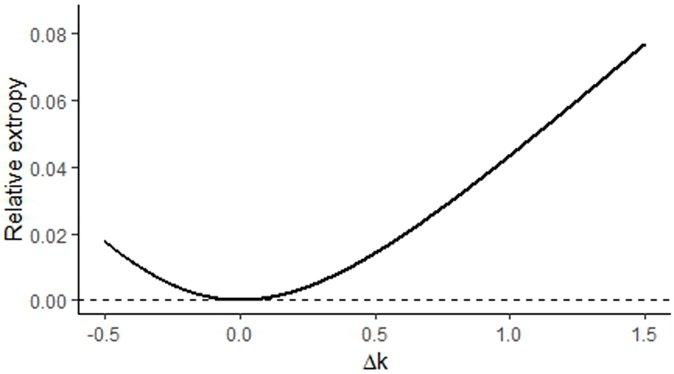


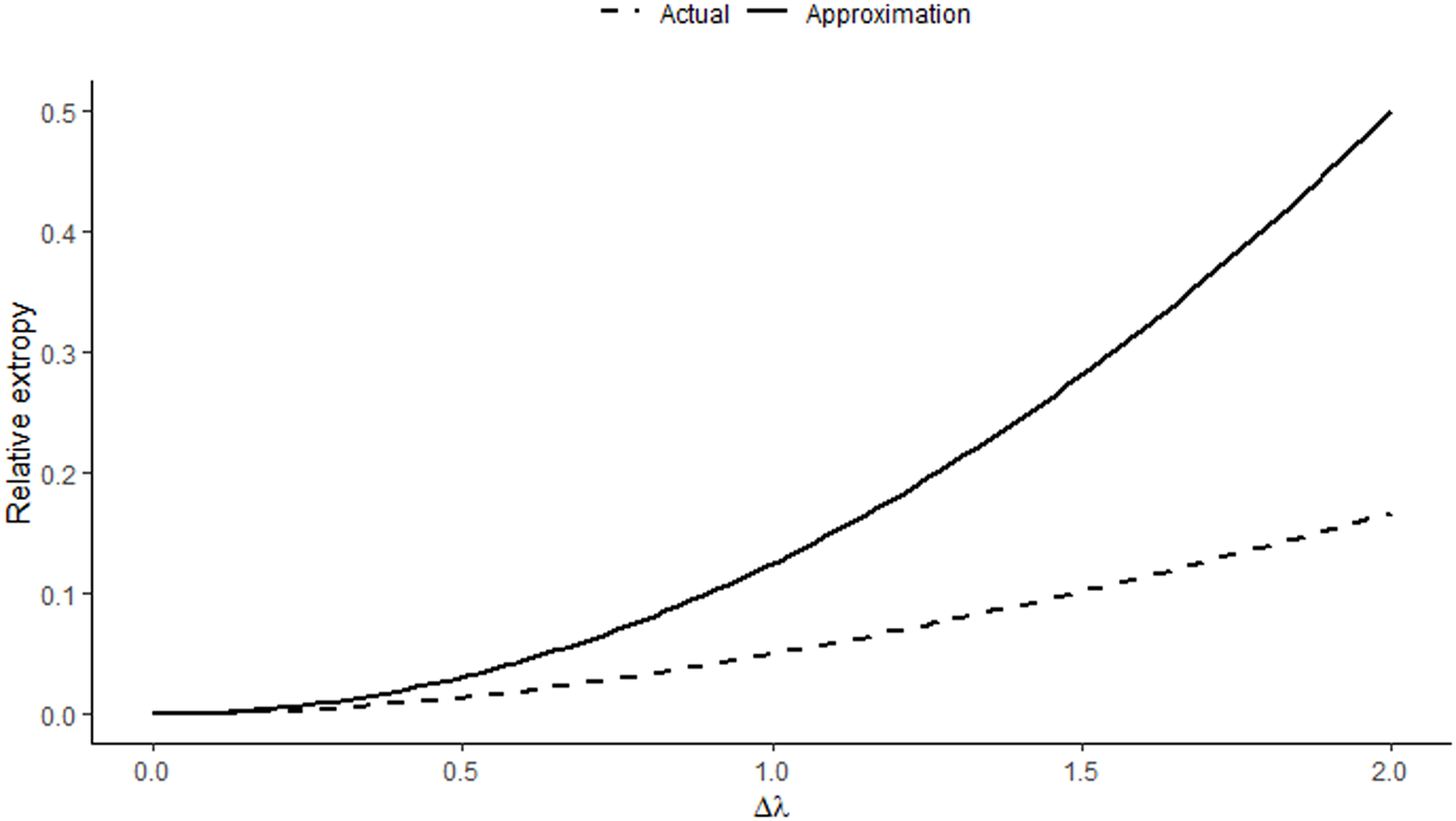

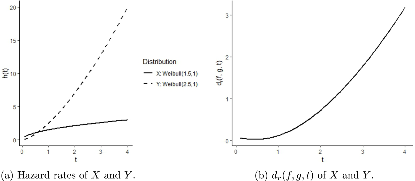


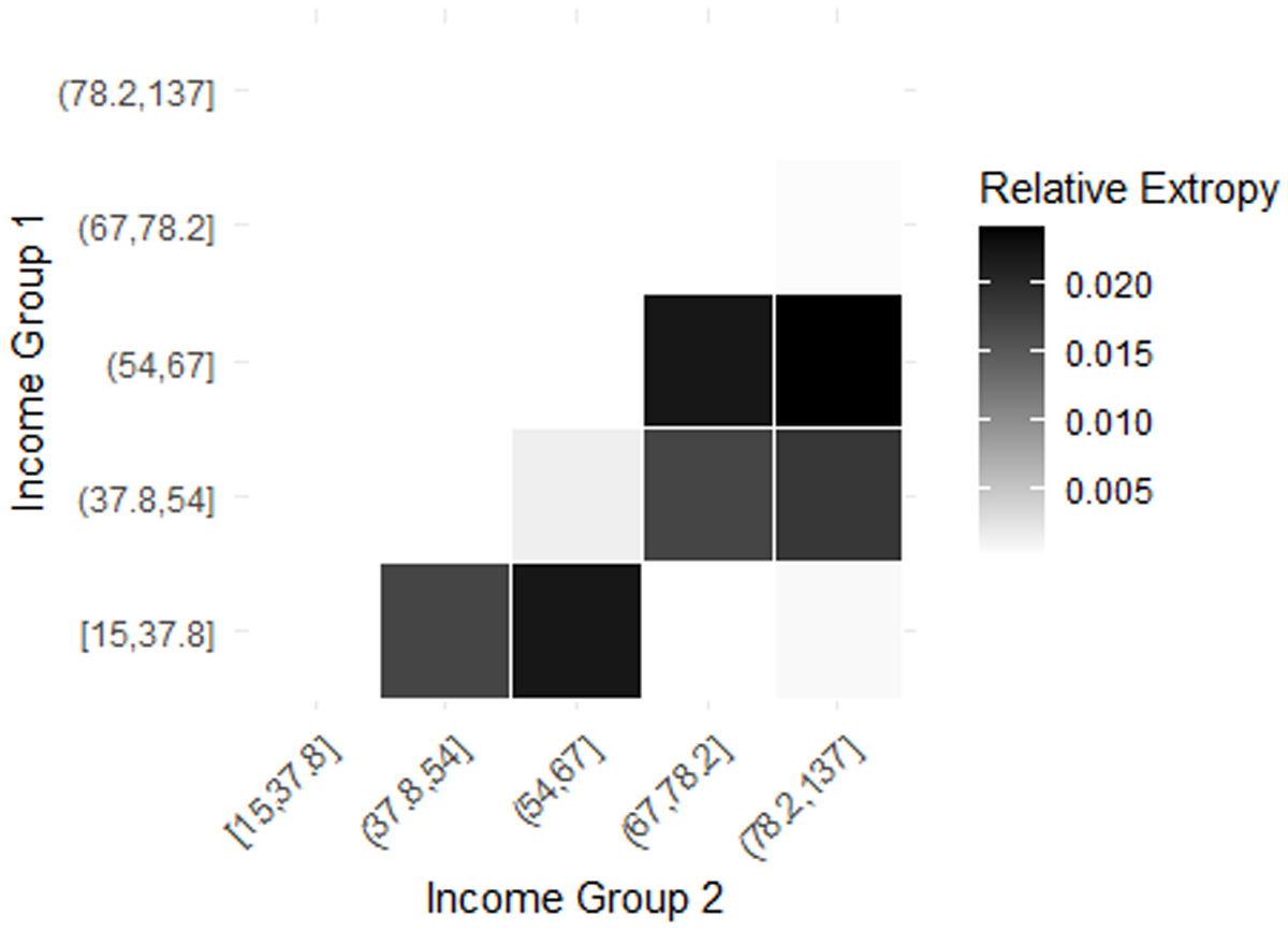


 Open access