


1. Introduction
In the study of coherent systems in reliability theory, the notion of signature, introduced originally by Samaniego [Reference Samaniego13], has become a key tool in examining reliability properties, assessing better system structures, and developing inferential procedures based on system lifetime data; see Kochar et al. [Reference Kochar, Mukerjee and Samaniego9], Shaked and Suarez-Llorens [Reference Shaked and Suarez-Llorens16], Balakrishnan et al. [Reference Balakrishnan, Ng and Navarro1, Reference Balakrishnan, Ng and Navarro2], and Izadkhah et al. [Reference Izadkhah, Amini-Seresht and Balakrishnan8]. Furthermore, based on this signature, several other related notions such as survival signature, extended signature, joint signature, and ordered signature have also been introduced in the literature; see, for example, Coolen and Tahani-Maturi [Reference Coolen and Coolen-Maturi4], Navarro et al. [Reference Navarro, Ruiz and Sandoval11], Navarro et al. [Reference Navarro, Samaniego, Balakrishnan and Bhattacharya12], and Balakrishnan and Volterman [Reference Balakrishnan and Volterman3]. These notions have also been subsequently generalized to multi-state systems as can be seen, for example, in the works of Coolen and Tahani-Maturi [Reference Coolen, Coolen-Maturi, Zamojski, Mazurkiewicz, Sugier, Walkowiak and Kacprzyk5] and Yi et al. [Reference Yi, Balakrishnan and Cui17–Reference Yi, Balakrishnan and Li22]. For a comprehensive discussion on signatures and their applications, one may refer to the elaborate book by Samaniego [Reference Samaniego14].
It is worth stating that all the works mentioned above focused on coherent systems comprising components with continuous lifetimes. But, in practice, coherent systems comprising discrete components arise naturally in many circumstances when, for example, the systems are monitored only at discrete epoch times, or when the systems operate in cycles, and the observations are then the number of cycles completed successfully before the failure of the system.
Yet, for coherent systems with discrete component lifetimes, relatively few works exist, like the ones by Shaked et al. [Reference Shaked, Shanthikumar, Valdez-Torres and Özekici15], Fiondella and Xing [Reference Fiondella and Xing7], and Dembińska and Eryilmaz [Reference Dembinska and Eryilmaz6]. They also seem to deal with specific forms of systems rather than consider a general approach such as the one available through signatures in the continuous case.
For this reason, to fill this gap, we introduce here the notion of discrete-time signature to provide a general approach for studying coherent systems comprising independent components with discrete lifetimes, and then discuss some of its properties and associated results. The rest of this paper proceeds as follows. In Section 2, we first give the basic definition of the discrete-time signature, and then present the reliability function of the system based on it. In Section 3, some series and parallel systems are considered for understanding the discrete-time signature. In Section 4, we use it to establish a stochastic ordering result between the lifetimes of two coherent systems with discrete components. Next, in Section 5, we introduce transformation formula to facilitate the comparison of systems of different sizes. Finally, Section 6 presents some concluding remarks.
2. Definition and reliability function
First, let us recall the definition of signature in the continuous case, as given by Samaniego [Reference Samaniego13]. For a coherent system consisting of  $n$ components, let $T$ denote the system lifetime and $X_1, \ldots , X_n$ denote the lifetimes of the $n$ components. Then, when $X_i$’s are i.i.d. continuous random variables with a cumulative distribution function (cdf) $F(\cdot)$ and probability density function (pdf) $f(\cdot)$, the signature of the system is an $n$-dimensional vector $\boldsymbol{s} = (s_1, \ldots , s_n)$, with its $i$-th element $s_i = P(T=X_{i:n})$, where $X_{1:n} \leq \cdots \leq X_{n:n}$ are the order statistics corresponding to the lifetimes $X_1, \ldots , X_n$. In other words, $s_i$ is simply the probability that the $i$-th ordered component failure causes the failure of the system.
Remark 2.1. First thing to note in the above definition is that the failure of the system is at the failure of some component (due to the system being coherent). The second point is that the failure of the system can be caused by the failure of only one component (due to the assumption of continuous lifetimes for the components).
Remark 2.2. Naturally, when the lifetimes of components in a coherent system are discrete (like the number of successful cycles completed), the second point in the above Remark will not hold, while the first point will continue to hold due to the system being coherent.
A natural question that arises here then is as to how to define a signature in this discrete lifetime set-up. Intuitively, it is clear that we need to identify which ordered lifetime results in the failure of the system (just as in the continuous case), but also we need to specify the nature of ties among the lifetimes (due to the discreteness of the lifetimes). This intuition leads to the following definition of a discrete-time signature, which naturally is two-dimensional in nature and is therefore presented in the form of a matrix.
Definition 2.1. For a coherent system with  $n$ components and lifetime $T$, suppose the components have i.i.d. discrete lifetimes ${X_1}, \ldots ,{X_n}$ from a cdf $F(\cdot)$ and a probability mass function (pmf) $f(\cdot)$. Denoting the $i$-th smallest component lifetime by ${X_{i:n}}$, the signature of the system can be defined as
 \begin{equation*}\boldsymbol{s}=\left(s_i^{j_1,\dots,j_m},\;j_1+\cdots+j_m=n,\;1\leq i\leq m\leq n\right),\end{equation*}
where
 \begin{equation*}{s_{i}^{j_1,\ldots,j_m}} = P\{T = {X_{j_{(i-1)}+1 :n}}\left|{{E_{j_1,\ldots,j_m}}}\right.\} \end{equation*}
 is the conditional probability that failure of the system is caused by the  $j_{(i-1)+1}$-th component failure, given the event
 \begin{equation*}{E_{j_1,\ldots,j_m}}=\{X_{(1,\ldots,j_{(1)}):n} \lt {X_{(j_{(1)}+1,\ldots,j_{(2)}):n}} \lt \cdots \lt {X_{(j_{(m-1)} +1,\ldots,j_{(m)} ):n}}\},\end{equation*}
 where  ${j_1},\ldots,{j_m}$ are the numbers of order statistics $X_{1:n},\ldots,X_{n:n}$ that are equal to the first, second, $\ldots$, $m$-th distinct values, respectively. Here, ${X_{(u,\ldots,v):n}}$ is an abbreviation for ${X_{u:n}}=\cdots={X_{v:n}}$ ( $1\le u \le v\le n$) and $j_{(i)}={j_1}+\cdots+{j_i}$ is the $i$-th partial sum for $i=1,\ldots,m$. It is clear that $j_{(1)}=j_1$ and $j_{(m)}=\sum\nolimits_{i=1}^{m} {j_i} =n$. Without loss of generality, we set $j_{(0)}=0$ and $j_{(-1)} =-1$.
Remark 2.3. It is useful to observe that the discrete-time signature is distribution-free, namely, the elements  ${s_{i}^{j_1,\ldots,j_m}}$ do not depend on the components’ lifetime distribution $F$. Besides, note that $\sum\nolimits_{i=1}^m{s_{i}^{j_1,\ldots,j_m}}=1$ holds for all $j_1 +\cdots +j_m= n$ ( $1\le m\le n$), which is due to the fact that the discrete-time signature has been defined based on conditional events ${E_{j_1,\ldots,j_m}}$. If not, we can redefine the discrete-time signature in an unconditional way, namely, we can set
 \begin{equation*}s_i^{j_1,\dots,j_m}=P\{T=X_{j_{(i-1)}+1:n},\;E_{j_1,\dots,j_m}\},\end{equation*}
 which would lead to  $\sum\nolimits_{j_1 +\cdots +j_m= n}\sum\nolimits_{i=1}^m{s_{i}^{j_1,\ldots,j_m}}=1$ instead.
Remark 2.4. The discrete-time signature can be regarded as a matrix of dimension  $C_n\times n$, where
  $C_n=\sum\limits_{m = 1}^n {\left( {\begin{matrix}
{n - 1} \\
{m - 1} \end{matrix} } \right)}=2^{n-1} $ is the total number of compositions (i.e., distinguishable partitions) of an integer
$C_n=\sum\limits_{m = 1}^n {\left( {\begin{matrix}
{n - 1} \\
{m - 1} \end{matrix} } \right)}=2^{n-1} $ is the total number of compositions (i.e., distinguishable partitions) of an integer  $n$. For example, consider a $2$-out-of- $3$: F system. Its discrete-time signature can be regarded as a matrix of dimension $C_3\times 3$ with
  $C_3=\left( {\begin{matrix}
{2} \\
{0} \end{matrix} } \right)+\left( {\begin{matrix}
{2} \\
{1} \end{matrix} } \right)+\left( {\begin{matrix}
{2} \\
{2} \end{matrix} } \right)=4$ as follows:
$C_3=\left( {\begin{matrix}
{2} \\
{0} \end{matrix} } \right)+\left( {\begin{matrix}
{2} \\
{1} \end{matrix} } \right)+\left( {\begin{matrix}
{2} \\
{2} \end{matrix} } \right)=4$ as follows:
 \begin{align*}
\boldsymbol s=\left( {\begin{matrix}
{s_1^{1,1,1}} & {s_2^{1,1,1}} &{s_3^{1,1,1}} \\
{s_1^{1,2}} & {s_2^{1,2}} & 0 \\
{s_1^{2,1}} & {s_2^{2,1}} & 0 \\
{s_1^{3}} & 0 & 0
\end{matrix} } \right)=\left( {\begin{matrix}
0 & 1 & 0\\
0 & 1 & 0 \\
1 & 0 & 0 \\
1 & 0 & 0
\end{matrix} } \right).
\end{align*}
\begin{align*}
\boldsymbol s=\left( {\begin{matrix}
{s_1^{1,1,1}} & {s_2^{1,1,1}} &{s_3^{1,1,1}} \\
{s_1^{1,2}} & {s_2^{1,2}} & 0 \\
{s_1^{2,1}} & {s_2^{2,1}} & 0 \\
{s_1^{3}} & 0 & 0
\end{matrix} } \right)=\left( {\begin{matrix}
0 & 1 & 0\\
0 & 1 & 0 \\
1 & 0 & 0 \\
1 & 0 & 0
\end{matrix} } \right).
\end{align*} Observe that the first row of the discrete-time signature matrix  $\boldsymbol s$, which corresponds to the case ${j_1} = \cdots = {j_m} = 1$ ( $m=n$), can be written as $(s_1^{1, \ldots 1}, \ldots ,s_n^{1, \ldots 1})$ with
 \begin{equation*}s_i^{1, \ldots 1} = P\{T = {X_{i:n}}\left| {{X_{1:n}} \lt {X_{2:n}} \lt \cdots \lt {X_{n:n}}} \right.\} ,{\rm{~~~~ }}i = 1, \ldots ,n.\end{equation*}
 That is exactly the continuous-time signature for the same coherent system, because the conditional probability  $s_i^{1,\ldots,1}$ should be the same as the probability $P\{T = {X_{i:n}}\}$ in continuous-time case due to the fact that both the discrete-time signature and the continuous-time signature are distribution-free and they can be evaluated in the same way by considering all permutations of component lifetimes; see Examples 3.1 and 3.3 for relevant details.
The above definition of discrete signature can be used readily to present the following proposition.
Proposition 2.1. The pmf of the system lifetime  $T$ can be given as
 \begin{equation*} P\{T = t\} = \sum\limits_{m=1}^n\sum\limits_{j_1 +\cdots +j_m= n}\left( {\begin{matrix}
n \\
{j_1,\ldots,j_m} \end{matrix} } \right) \sum\limits_{i = 1}^{m} {s_{i}^{j_1,\ldots,j_m}} \left[ \sum_{\scriptstyle 1 \le {t_1} \lt \cdots \lt {t_i} = \atop \scriptstyle t \lt \cdots \lt {t_m} \lt \infty } {{\prod\limits_{u = 1}^m {{f^{{j_u}}}({t_u})} } } \right] ,\end{equation*}
\begin{equation*} P\{T = t\} = \sum\limits_{m=1}^n\sum\limits_{j_1 +\cdots +j_m= n}\left( {\begin{matrix}
n \\
{j_1,\ldots,j_m} \end{matrix} } \right) \sum\limits_{i = 1}^{m} {s_{i}^{j_1,\ldots,j_m}} \left[ \sum_{\scriptstyle 1 \le {t_1} \lt \cdots \lt {t_i} = \atop \scriptstyle t \lt \cdots \lt {t_m} \lt \infty } {{\prod\limits_{u = 1}^m {{f^{{j_u}}}({t_u})} } } \right] ,\end{equation*}the survival function as
 \begin{equation*}P\{T \gt t\}=\sum_{m=1}^n\sum_{j_1+\cdots+j_m=n}\begin{pmatrix}n\\j_1,\dots,j_m\end{pmatrix}\sum_{i=0}^{m-1}\left(\sum_{l=i+1}^ms_l^{j_1,\dots,j_m}\right)\left[\sum_{\textstyle\begin{array}{c}1\leq t_1 \lt \cdots \lt t_i\leq t \lt \\t_{i+1} \lt \cdots \lt t_m \lt \infty\end{array}}\prod_{u=1}^m{f^{j_u}(t_u)}\right],\end{equation*}
and the cumulative distribution function as
 \begin{equation*}P\{T\leq t\}=\sum_{m=1}^n\sum_{j_1+\cdots+j_m=n}\begin{pmatrix}n\\j_1,\dots,j_m\end{pmatrix}\sum_{i=1}^m\left(\sum_{l=1}^is_l^{j_1,\dots,j_m}\right)\left[\sum_{\textstyle\begin{array}{c}1\leq t_1 \lt \cdots \lt t_i\leq t \lt \\t_{i+1} \lt \cdots \lt t_m \lt \infty\end{array}}\prod_{u=1}^m{f^{j_u}(t_u)}\right].\end{equation*}
Proof. According to Definition 2.1, we have
 \begin{align*}
P\{T = t\} & =\sum\limits_{m=1}^n \sum\limits_{j_1 +\cdots +j_m= n} {\sum\limits_{i = 1}^{m} {P\{T =t\left|T = {X_{j_{(i-1)}+1 :n}},~E_{j_1,\ldots,j_m}\right.\} } } \cdot P\{T = {X_{j_{(i-1)}+1 :n}},~{E_{j_1,\ldots,j_m}}\} \\
& =\sum\limits_{m=1}^n \sum\limits_{j_1 +\cdots +j_m= n} {\sum\limits_{i = 1}^{m} {P\{{X_{j_{(i-1)}+1 :n}} =t\left|E_{j_1,\ldots,j_m}\right.\} } } \cdot {s_{i}^{j_1,\ldots,j_m}} \cdot P\{E_{j_1,\ldots,j_m}\} \\
& =\sum\limits_{m=1}^n \sum\limits_{j_1 +\cdots +j_m= n} {\sum\limits_{i = 1}^{m} {{s_{i}^{j_1,\ldots,j_m}} \cdot P\{{X_{j_{(i-1)}+1 :n}} =t,~ E_{j_1,\ldots,j_m}\} } }, \\
P\{T \gt t\} & = \sum\limits_{m=1}^n\sum\limits_{j_1 +\cdots +j_m= n} {\sum\limits_{l = 1}^{m} {P\{T \gt t\left|T = {X_{j_{(l-1)}+1 :n}},~E_{j_1,\ldots,j_m}\right.\} } } \cdot P\{T = {X_{j_{(l-1)}+1 :n}},~{E_{j_1,\ldots,j_m}}\} \\
& = \sum\limits_{m=1}^n\sum\limits_{j_1 +\cdots +j_m= n} {\sum\limits_{l = 1}^{m} {P\{{X_{j_{(l-1)} +1:n}} \gt t\left|E_{j_1,\ldots,j_m}\right.\} } } \cdot {s_{l}^{j_1,\ldots,j_m}} \cdot P\{E_{j_1,\ldots,j_m}\} \\
& =\sum\limits_{m=1}^n \sum\limits_{j_1 +\cdots +j_m= n} {\sum\limits_{l = 1}^{m} {{s_{l}^{j_1,\ldots,j_m}} \cdot P\{{X_{j_{(l-1)}+1 :n}} \gt t,~ E_{j_1,\ldots,j_m}\} } }\\
& =\sum\limits_{m=1}^n \sum\limits_{j_1 +\cdots +j_m= n} {\sum\limits_{l = 1}^{m} {{s_{l}^{j_1,\ldots,j_m}} \cdot \sum\limits_{i=0}^{l-1}P\{{X_{j_{(i-1)}+1 :n}} \le t \lt {X_{j_{(i)}+1 :n}},~ E_{j_1,\ldots,j_m}\} } }\\
&=\sum\limits_{m=1}^n \sum\limits_{j_1 +\cdots +j_m= n}
\sum\limits_{i=0}^{m-1} \left(\sum\limits_{l = i+1}^{m} {s_{l}^{j_1,\ldots,j_m}}\right) \cdot P\{{X_{j_{(i-1)} +1:n}} \le t \lt {X_{j_{(i)}+1 :n}},~ E_{j_1,\ldots,j_m}\} ,\end{align*}
\begin{align*}
P\{T = t\} & =\sum\limits_{m=1}^n \sum\limits_{j_1 +\cdots +j_m= n} {\sum\limits_{i = 1}^{m} {P\{T =t\left|T = {X_{j_{(i-1)}+1 :n}},~E_{j_1,\ldots,j_m}\right.\} } } \cdot P\{T = {X_{j_{(i-1)}+1 :n}},~{E_{j_1,\ldots,j_m}}\} \\
& =\sum\limits_{m=1}^n \sum\limits_{j_1 +\cdots +j_m= n} {\sum\limits_{i = 1}^{m} {P\{{X_{j_{(i-1)}+1 :n}} =t\left|E_{j_1,\ldots,j_m}\right.\} } } \cdot {s_{i}^{j_1,\ldots,j_m}} \cdot P\{E_{j_1,\ldots,j_m}\} \\
& =\sum\limits_{m=1}^n \sum\limits_{j_1 +\cdots +j_m= n} {\sum\limits_{i = 1}^{m} {{s_{i}^{j_1,\ldots,j_m}} \cdot P\{{X_{j_{(i-1)}+1 :n}} =t,~ E_{j_1,\ldots,j_m}\} } }, \\
P\{T \gt t\} & = \sum\limits_{m=1}^n\sum\limits_{j_1 +\cdots +j_m= n} {\sum\limits_{l = 1}^{m} {P\{T \gt t\left|T = {X_{j_{(l-1)}+1 :n}},~E_{j_1,\ldots,j_m}\right.\} } } \cdot P\{T = {X_{j_{(l-1)}+1 :n}},~{E_{j_1,\ldots,j_m}}\} \\
& = \sum\limits_{m=1}^n\sum\limits_{j_1 +\cdots +j_m= n} {\sum\limits_{l = 1}^{m} {P\{{X_{j_{(l-1)} +1:n}} \gt t\left|E_{j_1,\ldots,j_m}\right.\} } } \cdot {s_{l}^{j_1,\ldots,j_m}} \cdot P\{E_{j_1,\ldots,j_m}\} \\
& =\sum\limits_{m=1}^n \sum\limits_{j_1 +\cdots +j_m= n} {\sum\limits_{l = 1}^{m} {{s_{l}^{j_1,\ldots,j_m}} \cdot P\{{X_{j_{(l-1)}+1 :n}} \gt t,~ E_{j_1,\ldots,j_m}\} } }\\
& =\sum\limits_{m=1}^n \sum\limits_{j_1 +\cdots +j_m= n} {\sum\limits_{l = 1}^{m} {{s_{l}^{j_1,\ldots,j_m}} \cdot \sum\limits_{i=0}^{l-1}P\{{X_{j_{(i-1)}+1 :n}} \le t \lt {X_{j_{(i)}+1 :n}},~ E_{j_1,\ldots,j_m}\} } }\\
&=\sum\limits_{m=1}^n \sum\limits_{j_1 +\cdots +j_m= n}
\sum\limits_{i=0}^{m-1} \left(\sum\limits_{l = i+1}^{m} {s_{l}^{j_1,\ldots,j_m}}\right) \cdot P\{{X_{j_{(i-1)} +1:n}} \le t \lt {X_{j_{(i)}+1 :n}},~ E_{j_1,\ldots,j_m}\} ,\end{align*}and
 \begin{align*}
P\{T \le t\} & =\sum\limits_{m=1}^n \sum\limits_{j_1 +\cdots +j_m= n} {\sum\limits_{l = 1}^{m} {P\{T \le t\left|T = {X_{j_{(l-1)}+1 :n}},~E_{j_1,\ldots,j_m}\right.\} } } \cdot P\{T = {X_{j_{(l-1)}+1 :n}},~{E_{j_1,\ldots,j_m}}\} \\
& =\sum\limits_{m=1}^n \sum\limits_{j_1 +\cdots +j_m= n} {\sum\limits_{l = 1}^{m} {P\{{X_{j_{(l-1)}+1 :n}} \le t\left|E_{j_1,\ldots,j_m}\right.\} } } \cdot {s_{l}^{j_1,\ldots,j_m}} \cdot P\{E_{j_1,\ldots,j_m}\} \\
& =\sum\limits_{m=1}^n \sum\limits_{j_1 +\cdots +j_m= n} {\sum\limits_{l = 1}^{m} {{s_{l}^{j_1,\ldots,j_m}} \cdot P\{{X_{j_{(l-1)}+1 :n}} \le t,~ E_{j_1,\ldots,j_m}\} } }\\
& =\sum\limits_{m=1}^n \sum\limits_{j_1 +\cdots +j_m= n} {\sum\limits_{l = 1}^{m} {{s_{l}^{j_1,\ldots,j_m}} \cdot \sum\limits_{i=l}^{m}P\{{X_{j_{(i-1)} +1:n}} \le t \lt {X_{j_{(i)}+1 :n}},~ E_{j_1,\ldots,j_m}\} } }\\
&= \sum\limits_{m=1}^n\sum\limits_{j_1 +\cdots +j_m= n}
\sum\limits_{i=1}^{m} \left(\sum\limits_{l = 1}^{i} {s_{l}^{j_1,\ldots,j_m}}\right) \cdot P\{{X_{j_{(i-1)}+1 :n}} \le t \lt {X_{j_{(i)}+1 :n}},~ E_{j_1,\ldots,j_m}\} ,
\end{align*}
\begin{align*}
P\{T \le t\} & =\sum\limits_{m=1}^n \sum\limits_{j_1 +\cdots +j_m= n} {\sum\limits_{l = 1}^{m} {P\{T \le t\left|T = {X_{j_{(l-1)}+1 :n}},~E_{j_1,\ldots,j_m}\right.\} } } \cdot P\{T = {X_{j_{(l-1)}+1 :n}},~{E_{j_1,\ldots,j_m}}\} \\
& =\sum\limits_{m=1}^n \sum\limits_{j_1 +\cdots +j_m= n} {\sum\limits_{l = 1}^{m} {P\{{X_{j_{(l-1)}+1 :n}} \le t\left|E_{j_1,\ldots,j_m}\right.\} } } \cdot {s_{l}^{j_1,\ldots,j_m}} \cdot P\{E_{j_1,\ldots,j_m}\} \\
& =\sum\limits_{m=1}^n \sum\limits_{j_1 +\cdots +j_m= n} {\sum\limits_{l = 1}^{m} {{s_{l}^{j_1,\ldots,j_m}} \cdot P\{{X_{j_{(l-1)}+1 :n}} \le t,~ E_{j_1,\ldots,j_m}\} } }\\
& =\sum\limits_{m=1}^n \sum\limits_{j_1 +\cdots +j_m= n} {\sum\limits_{l = 1}^{m} {{s_{l}^{j_1,\ldots,j_m}} \cdot \sum\limits_{i=l}^{m}P\{{X_{j_{(i-1)} +1:n}} \le t \lt {X_{j_{(i)}+1 :n}},~ E_{j_1,\ldots,j_m}\} } }\\
&= \sum\limits_{m=1}^n\sum\limits_{j_1 +\cdots +j_m= n}
\sum\limits_{i=1}^{m} \left(\sum\limits_{l = 1}^{i} {s_{l}^{j_1,\ldots,j_m}}\right) \cdot P\{{X_{j_{(i-1)}+1 :n}} \le t \lt {X_{j_{(i)}+1 :n}},~ E_{j_1,\ldots,j_m}\} ,
\end{align*} where \begin{align*}
& P\{{X_{j_{(i-1)}+1 :n}} =t,~ E_{j_1,\ldots,j_m}\} = \left( {\begin{matrix}
n \\
{j_1,\ldots,j_m} \end{matrix} } \right)\left[ \sum\limits_{\scriptstyle 1 \le {t_1} \lt \cdots \lt {t_i}=\atop \scriptstyle t \lt \cdots \lt {t_m} \lt \infty } {{\prod\limits_{u = 1}^m {{f^{{j_u}}}({t_u})} } } \right] , \\
& P\{{X_{j_{(i-1)}+1 :n}} \le t \lt {X_{j_{(i)}+1 :n}},~ E_{j_1,\ldots,j_m}\} = \left( {\begin{matrix}
n \\
{j_1,\ldots,j_m} \end{matrix} } \right)\left[ \sum\limits_{\scriptstyle 1 \le {t_1} \lt \cdots \lt {t_i} \le t \lt \atop \scriptstyle \lt t_{i+1} \cdots \lt {t_m} \lt \infty } {{\prod\limits_{u = 1}^m {{f^{{j_u}}}({t_u})}}} \right] .
\end{align*}
\begin{align*}
& P\{{X_{j_{(i-1)}+1 :n}} =t,~ E_{j_1,\ldots,j_m}\} = \left( {\begin{matrix}
n \\
{j_1,\ldots,j_m} \end{matrix} } \right)\left[ \sum\limits_{\scriptstyle 1 \le {t_1} \lt \cdots \lt {t_i}=\atop \scriptstyle t \lt \cdots \lt {t_m} \lt \infty } {{\prod\limits_{u = 1}^m {{f^{{j_u}}}({t_u})} } } \right] , \\
& P\{{X_{j_{(i-1)}+1 :n}} \le t \lt {X_{j_{(i)}+1 :n}},~ E_{j_1,\ldots,j_m}\} = \left( {\begin{matrix}
n \\
{j_1,\ldots,j_m} \end{matrix} } \right)\left[ \sum\limits_{\scriptstyle 1 \le {t_1} \lt \cdots \lt {t_i} \le t \lt \atop \scriptstyle \lt t_{i+1} \cdots \lt {t_m} \lt \infty } {{\prod\limits_{u = 1}^m {{f^{{j_u}}}({t_u})}}} \right] .
\end{align*}
Hence, the proposition.
Remark 2.5. In the case of Geometric( $p$) distribution with pmf $f(t)=pq^{t-1},~t=1,\ldots,\infty,~q=1-p$, we can derive the following expression explicitly:
 \begin{align*}
& P\{E_{j_1,\ldots,j_m}\} = \left( {\begin{matrix}
n \\
{j_1,\ldots,j_m} \end{matrix} } \right)\left[ \sum\limits_{1 \le {t_1} \lt \cdots \lt {t_m} \lt \infty } {{\prod\limits_{u = 1}^m {p^{j_u}q^{{j_u}({t_u}-1)}} } } \right] ,
\end{align*}
\begin{align*}
& P\{E_{j_1,\ldots,j_m}\} = \left( {\begin{matrix}
n \\
{j_1,\ldots,j_m} \end{matrix} } \right)\left[ \sum\limits_{1 \le {t_1} \lt \cdots \lt {t_m} \lt \infty } {{\prod\limits_{u = 1}^m {p^{j_u}q^{{j_u}({t_u}-1)}} } } \right] ,
\end{align*}where
 \begin{align*}
&\sum\limits_{1 \le {t_1} \lt \cdots \lt {t_m} \lt \infty} {{\prod\limits_{u = 1}^m {p^{j_u}q^{{j_u}({t_u}-1)}} }} \\
&= \sum\limits_{1 \le {t_1} \lt \cdots \lt {t_{m-1}} \lt \infty} {{\prod\limits_{u = 1}^{m-1} {p^{j_u}q^{{j_u}({t_u}-1)}} }} \sum\limits_{t_{m}={t_{m-1}+1}}^{\infty}{{p^{j_m}q^{{j_m}({t_m}-1)}}}\\
&= {q^{j_m}\over{1-q^{j_m}}}\sum\limits_{1 \le {t_1} \lt \cdots \lt {t_{m-1}} \lt \infty} {\left( {\prod\limits_{u = 1}^{m-2} {p^{j_u}q^{{j_u}({t_u}-1)}} }\right)}{{p^{j_{m-1}+j_m}q^{({j_{m-1}+j_m})({t_{m-1}}-1)}}}\\
&=\left(\prod\limits_{u = 2}^m {{{{q^{{j_u} + \cdots + {j_m}}}} \over {1 - {q^{{j_u} + \cdots + {j_m}}}}}}\right)\sum\limits_{1 \le {t_1} \lt \infty } {{p^{j_{1}+\cdots+j_m}q^{({j_{1}+\cdots+j_m})({t_{1}}-1)}}}\\
&=\left(\prod\limits_{u = 2}^m {{{{q^{{j_{(m)}} - {j_{(u-1)}}}}} \over {1 - {q^{{j_{(m)}} - {j_{(u-1)}}}}}}}\right){{{{p^{n}}} \over {1 - {q^{n}}}}}.
\end{align*}
\begin{align*}
&\sum\limits_{1 \le {t_1} \lt \cdots \lt {t_m} \lt \infty} {{\prod\limits_{u = 1}^m {p^{j_u}q^{{j_u}({t_u}-1)}} }} \\
&= \sum\limits_{1 \le {t_1} \lt \cdots \lt {t_{m-1}} \lt \infty} {{\prod\limits_{u = 1}^{m-1} {p^{j_u}q^{{j_u}({t_u}-1)}} }} \sum\limits_{t_{m}={t_{m-1}+1}}^{\infty}{{p^{j_m}q^{{j_m}({t_m}-1)}}}\\
&= {q^{j_m}\over{1-q^{j_m}}}\sum\limits_{1 \le {t_1} \lt \cdots \lt {t_{m-1}} \lt \infty} {\left( {\prod\limits_{u = 1}^{m-2} {p^{j_u}q^{{j_u}({t_u}-1)}} }\right)}{{p^{j_{m-1}+j_m}q^{({j_{m-1}+j_m})({t_{m-1}}-1)}}}\\
&=\left(\prod\limits_{u = 2}^m {{{{q^{{j_u} + \cdots + {j_m}}}} \over {1 - {q^{{j_u} + \cdots + {j_m}}}}}}\right)\sum\limits_{1 \le {t_1} \lt \infty } {{p^{j_{1}+\cdots+j_m}q^{({j_{1}+\cdots+j_m})({t_{1}}-1)}}}\\
&=\left(\prod\limits_{u = 2}^m {{{{q^{{j_{(m)}} - {j_{(u-1)}}}}} \over {1 - {q^{{j_{(m)}} - {j_{(u-1)}}}}}}}\right){{{{p^{n}}} \over {1 - {q^{n}}}}}.
\end{align*}Remark 2.6. In the case of Geometric( $p$) distribution with pmf $f(t)=pq^{t-1},~t=1,\ldots,\infty,~q=1-p$, we can similarly derive the following explicit expression:
 \begin{align*}
& P\{{X_{j_{(i-1)}+1 :n}} =t,~ E_{j_1,\ldots,j_m}\} = \left( {\begin{matrix}
n \\
{j_1,\ldots,j_m} \end{matrix} } \right)\left[ \sum\limits_{\scriptstyle 1 \le {t_1} \lt \cdots \lt {t_i}= \atop \scriptstyle t \lt \cdots \lt {t_m} \lt \infty} {{\prod\limits_{u = 1}^m {p^{j_u}q^{{j_u}({t_u}-1)}} } } \right] ,
\end{align*}
\begin{align*}
& P\{{X_{j_{(i-1)}+1 :n}} =t,~ E_{j_1,\ldots,j_m}\} = \left( {\begin{matrix}
n \\
{j_1,\ldots,j_m} \end{matrix} } \right)\left[ \sum\limits_{\scriptstyle 1 \le {t_1} \lt \cdots \lt {t_i}= \atop \scriptstyle t \lt \cdots \lt {t_m} \lt \infty} {{\prod\limits_{u = 1}^m {p^{j_u}q^{{j_u}({t_u}-1)}} } } \right] ,
\end{align*}where
 \begin{align*}
&\sum\limits_{1 \le {t_1} \lt \cdots \lt {t_i}= t \lt \cdots \lt {t_m} \lt \infty} {{\prod\limits_{u = 1}^m {p^{j_u}q^{{j_u}({t_u}-1)}} }} \\
&= \sum\limits_{1 \le {t_1} \lt \cdots \lt {t_i}= t \lt \cdots \lt {t_{m-1}} \lt \infty} {{\prod\limits_{u = 1}^{m-1} {p^{j_u}q^{{j_u}({t_u}-1)}} }} \sum\limits_{t_{m}={t_{m-1}+1}}^{\infty}{{p^{j_m}q^{{j_m}({t_m}-1)}}}\\
&= {q^{j_m}\over{1-q^{j_m}}}\sum\limits_{1 \le {t_1} \lt \cdots \lt {t_i}= t \lt \cdots \lt {t_{m-1}} \lt \infty} {\left( {\prod\limits_{u = 1}^{m-2} {p^{j_u}q^{{j_u}({t_u}-1)}} }\right)}{{p^{j_{m-1}+j_m}q^{({j_{m-1}+j_m})({t_{m-1}}-1)}}}\\
&=\left(\prod\limits_{u = i + 1}^m {{{{q^{{j_u} + \cdots + {j_m}}}} \over {1 - {q^{{j_u} + \cdots + {j_m}}}}}}\right)^{I_{\{i\le m-1\}}}\sum\limits_{1 \le {t_1} \lt \cdots \lt {t_i}= t } {\left( {\prod\limits_{u = 1}^{i-1} {p^{j_u}q^{{j_u}({t_u}-1)}} }\right)}{{p^{j_{i}+\cdots+j_m}q^{({j_{i}+\cdots+j_m})({t_{i}}-1)}}}\\
&=\left(\prod\limits_{u = i + 1}^m {{{{q^{{j_{(m)}} - {j_{(u-1)}}}}} \over {1 - {q^{{j_{(m)}} - {j_{(u-1)}}}}}}}\right)^{I_{\{i\le m-1\}}}{{p^{j_{(m)}-j_{(i-1)}}q^{({j_{(m)}-j_{(i-1)}})(t-1)}}}\sum\limits_{1 \le {t_1} \lt \cdots \lt {t_{i-1}} \lt t } {\left( {\prod\limits_{u = 1}^{i-1} {p^{j_u}q^{{j_u}({t_u}-1)}} }\right)}.
\end{align*}
\begin{align*}
&\sum\limits_{1 \le {t_1} \lt \cdots \lt {t_i}= t \lt \cdots \lt {t_m} \lt \infty} {{\prod\limits_{u = 1}^m {p^{j_u}q^{{j_u}({t_u}-1)}} }} \\
&= \sum\limits_{1 \le {t_1} \lt \cdots \lt {t_i}= t \lt \cdots \lt {t_{m-1}} \lt \infty} {{\prod\limits_{u = 1}^{m-1} {p^{j_u}q^{{j_u}({t_u}-1)}} }} \sum\limits_{t_{m}={t_{m-1}+1}}^{\infty}{{p^{j_m}q^{{j_m}({t_m}-1)}}}\\
&= {q^{j_m}\over{1-q^{j_m}}}\sum\limits_{1 \le {t_1} \lt \cdots \lt {t_i}= t \lt \cdots \lt {t_{m-1}} \lt \infty} {\left( {\prod\limits_{u = 1}^{m-2} {p^{j_u}q^{{j_u}({t_u}-1)}} }\right)}{{p^{j_{m-1}+j_m}q^{({j_{m-1}+j_m})({t_{m-1}}-1)}}}\\
&=\left(\prod\limits_{u = i + 1}^m {{{{q^{{j_u} + \cdots + {j_m}}}} \over {1 - {q^{{j_u} + \cdots + {j_m}}}}}}\right)^{I_{\{i\le m-1\}}}\sum\limits_{1 \le {t_1} \lt \cdots \lt {t_i}= t } {\left( {\prod\limits_{u = 1}^{i-1} {p^{j_u}q^{{j_u}({t_u}-1)}} }\right)}{{p^{j_{i}+\cdots+j_m}q^{({j_{i}+\cdots+j_m})({t_{i}}-1)}}}\\
&=\left(\prod\limits_{u = i + 1}^m {{{{q^{{j_{(m)}} - {j_{(u-1)}}}}} \over {1 - {q^{{j_{(m)}} - {j_{(u-1)}}}}}}}\right)^{I_{\{i\le m-1\}}}{{p^{j_{(m)}-j_{(i-1)}}q^{({j_{(m)}-j_{(i-1)}})(t-1)}}}\sum\limits_{1 \le {t_1} \lt \cdots \lt {t_{i-1}} \lt t } {\left( {\prod\limits_{u = 1}^{i-1} {p^{j_u}q^{{j_u}({t_u}-1)}} }\right)}.
\end{align*} Denote  $A(i,t)=\sum\limits_{1 \le {t_1} \lt \cdots \lt {t_i}\le t } {\left( {\prod\limits_{u = 1}^{i} {p^{j_u}q^{{j_u}({t_u}-1)}} }\right)}$ for $i=1,\ldots,n,~t=1,\ldots,\infty$. Then, we have
 \begin{align*}
A(i,t)&=\sum\limits_{1 \le {t_1} \lt \cdots \lt {t_{i-1}}\le t-1} {\left( {\prod\limits_{u = 1}^{i-1} {p^{j_u}q^{{j_u}({t_u}-1)}} }\right)}\sum\limits_{t_i=t_{i-1}+1}^{t}{p^{j_i}q^{{j_i}({t_i}-1)}}\\
&={p{^{j_i}}\over{1-q^{{j_i}}}}\sum\limits_{1 \le {t_1} \lt \cdots \lt {t_{i-1}}\le t-1 } {\left( {\prod\limits_{u = 1}^{i-1} {p^{j_u}q^{{j_u}({t_u}-1)}} }\right)}({q^{{j_i}{t_{i-1}}}}-q^{{j_i}t})\\
&={q^{{j_i}}\over{1-q^{{j_i}}}}\sum\limits_{1 \le {t_1} \lt \cdots \lt {t_{i-1}}\le t-1 } {\left( {\prod\limits_{u = 1}^{i-1} {p^{j_u}q^{{j_u}({t_u}-1)}} }\right)}{p{^{j_i}}q^{{j_i}({t_{i-1}}-1)}}\\
&{\rm{~~~~}}-{p{^{j_i}}q^{j_it}\over{1-q^{{j_i}}}}\sum\limits_{1 \le {t_1} \lt \cdots \lt {t_{i-1}}\le t-1 } {\left( {\prod\limits_{u = 1}^{i-1} {p^{j_u}q^{{j_u}({t_u}-1)}} }\right)}\\
&={q^{{j_i}}\over{1-q^{{j_i}}}}B(i-1,t-1,j_i)-{p{^{j_i}}q^{j_it}\over{1-q^{{j_i}}}}A(i-1,t-1),\end{align*}
\begin{align*}
A(i,t)&=\sum\limits_{1 \le {t_1} \lt \cdots \lt {t_{i-1}}\le t-1} {\left( {\prod\limits_{u = 1}^{i-1} {p^{j_u}q^{{j_u}({t_u}-1)}} }\right)}\sum\limits_{t_i=t_{i-1}+1}^{t}{p^{j_i}q^{{j_i}({t_i}-1)}}\\
&={p{^{j_i}}\over{1-q^{{j_i}}}}\sum\limits_{1 \le {t_1} \lt \cdots \lt {t_{i-1}}\le t-1 } {\left( {\prod\limits_{u = 1}^{i-1} {p^{j_u}q^{{j_u}({t_u}-1)}} }\right)}({q^{{j_i}{t_{i-1}}}}-q^{{j_i}t})\\
&={q^{{j_i}}\over{1-q^{{j_i}}}}\sum\limits_{1 \le {t_1} \lt \cdots \lt {t_{i-1}}\le t-1 } {\left( {\prod\limits_{u = 1}^{i-1} {p^{j_u}q^{{j_u}({t_u}-1)}} }\right)}{p{^{j_i}}q^{{j_i}({t_{i-1}}-1)}}\\
&{\rm{~~~~}}-{p{^{j_i}}q^{j_it}\over{1-q^{{j_i}}}}\sum\limits_{1 \le {t_1} \lt \cdots \lt {t_{i-1}}\le t-1 } {\left( {\prod\limits_{u = 1}^{i-1} {p^{j_u}q^{{j_u}({t_u}-1)}} }\right)}\\
&={q^{{j_i}}\over{1-q^{{j_i}}}}B(i-1,t-1,j_i)-{p{^{j_i}}q^{j_it}\over{1-q^{{j_i}}}}A(i-1,t-1),\end{align*}where
 \begin{align*}
B(i,t,j_{i+1})&=\sum\limits_{1 \le {t_1} \lt \cdots \lt {t_{i}}\le t } {\left( {\prod\limits_{u = 1}^{i} {p^{j_u}q^{{j_u}({t_u}-1)}} }\right)}{p{^{j_{i+1}}}q^{{j_{i+1}}({t_{i}}-1)}}\\
&=\sum\limits_{1 \le {t_1} \lt \cdots \lt {t_{i-1}}\le t-1 } {\left( {\prod\limits_{u = 1}^{i-1} {p^{j_u}q^{{j_u}({t_u}-1)}} }\right)}\sum\limits_{t_i=t_{i-1}+1}^t{p{^{j_i+j_{i+1}}}q^{({j_i+j_{i+1})}({t_i}-1)}}\\
&={{p{^{j_i+j_{i+1}}}}\over {1-q^{j_i+j_{i+1}}}}\sum\limits_{1 \le {t_1} \lt \cdots \lt {t_{i-1}}\le t-1 } {\left( {\prod\limits_{u = 1}^{i-1} {p^{j_u}q^{{j_u}({t_u}-1)}} }\right)}[q^{({j_i+j_{i+1}}){t_{i-1}}}-q^{({j_i+j_{i+1}})t}]\\
&={{q{^{j_i+j_{i+1}}}}\over {1-q^{j_i+j_{i+1}}}}\sum\limits_{1 \le {t_1} \lt \cdots \lt {t_{i-1}}\le t-1 } {\left( {\prod\limits_{u = 1}^{i-1} {p^{j_u}q^{{j_u}({t_u}-1)}} }\right)}{p{^{j_i+j_{i+1}}}}q^{({j_i+j_{i+1}})({t_{i-1}}-1)}\\
&\quad-{{p{^{j_i+j_{i+1}}}}q^{({j_i+j_{i+1}})t}\over {1-q^{j_i+j_{i+1}}}}\sum\limits_{1 \le {t_1} \lt \cdots \lt {t_{i-1}}\le t-1 } {\left( {\prod\limits_{u = 1}^{i-1} {p^{j_u}q^{{j_u}({t_u}-1)}} }\right)}\\
&={{q{^{j_i+j_{i+1}}}}\over {1-q^{j_i+j_{i+1}}}}B(i-1,t-1,j_i+j_{i+1})-{{p{^{j_i+j_{i+1}}}}q^{({j_i+j_{i+1}})t}\over {1-q^{j_i+j_{i+1}}}}A(i-1,t-1),
\end{align*}
\begin{align*}
B(i,t,j_{i+1})&=\sum\limits_{1 \le {t_1} \lt \cdots \lt {t_{i}}\le t } {\left( {\prod\limits_{u = 1}^{i} {p^{j_u}q^{{j_u}({t_u}-1)}} }\right)}{p{^{j_{i+1}}}q^{{j_{i+1}}({t_{i}}-1)}}\\
&=\sum\limits_{1 \le {t_1} \lt \cdots \lt {t_{i-1}}\le t-1 } {\left( {\prod\limits_{u = 1}^{i-1} {p^{j_u}q^{{j_u}({t_u}-1)}} }\right)}\sum\limits_{t_i=t_{i-1}+1}^t{p{^{j_i+j_{i+1}}}q^{({j_i+j_{i+1})}({t_i}-1)}}\\
&={{p{^{j_i+j_{i+1}}}}\over {1-q^{j_i+j_{i+1}}}}\sum\limits_{1 \le {t_1} \lt \cdots \lt {t_{i-1}}\le t-1 } {\left( {\prod\limits_{u = 1}^{i-1} {p^{j_u}q^{{j_u}({t_u}-1)}} }\right)}[q^{({j_i+j_{i+1}}){t_{i-1}}}-q^{({j_i+j_{i+1}})t}]\\
&={{q{^{j_i+j_{i+1}}}}\over {1-q^{j_i+j_{i+1}}}}\sum\limits_{1 \le {t_1} \lt \cdots \lt {t_{i-1}}\le t-1 } {\left( {\prod\limits_{u = 1}^{i-1} {p^{j_u}q^{{j_u}({t_u}-1)}} }\right)}{p{^{j_i+j_{i+1}}}}q^{({j_i+j_{i+1}})({t_{i-1}}-1)}\\
&\quad-{{p{^{j_i+j_{i+1}}}}q^{({j_i+j_{i+1}})t}\over {1-q^{j_i+j_{i+1}}}}\sum\limits_{1 \le {t_1} \lt \cdots \lt {t_{i-1}}\le t-1 } {\left( {\prod\limits_{u = 1}^{i-1} {p^{j_u}q^{{j_u}({t_u}-1)}} }\right)}\\
&={{q{^{j_i+j_{i+1}}}}\over {1-q^{j_i+j_{i+1}}}}B(i-1,t-1,j_i+j_{i+1})-{{p{^{j_i+j_{i+1}}}}q^{({j_i+j_{i+1}})t}\over {1-q^{j_i+j_{i+1}}}}A(i-1,t-1),
\end{align*}and
 \begin{align*}
&A(1,t)=\sum\limits_{t_1=1 }^t {p^{j_1}q^{{j_1}({t_1}-1)}} ={{p^{j_1}(1-q^{j_1t})}\over {1-q^{j_1}}},\\
&B(1,t,j_2+\cdots+j_{i+1})=\sum\limits_{t_1=1}^t {{p^{j_1+\cdots+j_{i+1}}q^{{j_1+\cdots+j_{i+1}}({t_1}-1)}} }={{p^{j_1\cdots+j_{i+1}}(1-q^{(j_1+\cdots+j_{i+1})t})}\over {1-q^{j_1\cdots+j_{i+1}}}}.
\end{align*}
\begin{align*}
&A(1,t)=\sum\limits_{t_1=1 }^t {p^{j_1}q^{{j_1}({t_1}-1)}} ={{p^{j_1}(1-q^{j_1t})}\over {1-q^{j_1}}},\\
&B(1,t,j_2+\cdots+j_{i+1})=\sum\limits_{t_1=1}^t {{p^{j_1+\cdots+j_{i+1}}q^{{j_1+\cdots+j_{i+1}}({t_1}-1)}} }={{p^{j_1\cdots+j_{i+1}}(1-q^{(j_1+\cdots+j_{i+1})t})}\over {1-q^{j_1\cdots+j_{i+1}}}}.
\end{align*}We can now write
 \begin{align*}
&\left(\begin{matrix}
A(i,t)\\
B(i,t,j_{i+1})
\end{matrix}\right) =\boldsymbol P_{i,t}
\cdot\left(\begin{matrix}
A(i-1,t-1)\\
B(i-1,t-1,j_i+j_{i+1})
\end{matrix}\right)=\prod\limits_{u=0}^{i-1} \boldsymbol P_{i-u,t-u} \cdot\left(\begin{matrix}
A(1,t-i+1)\\
B(1,t-i+1,j_2+\cdots+j_{i+1})
\end{matrix}\right),
\end{align*}
\begin{align*}
&\left(\begin{matrix}
A(i,t)\\
B(i,t,j_{i+1})
\end{matrix}\right) =\boldsymbol P_{i,t}
\cdot\left(\begin{matrix}
A(i-1,t-1)\\
B(i-1,t-1,j_i+j_{i+1})
\end{matrix}\right)=\prod\limits_{u=0}^{i-1} \boldsymbol P_{i-u,t-u} \cdot\left(\begin{matrix}
A(1,t-i+1)\\
B(1,t-i+1,j_2+\cdots+j_{i+1})
\end{matrix}\right),
\end{align*} with  $
\boldsymbol P_{u,v}={\left(\begin{matrix}
-{p{^{j_u}}q^{j_uv}\over{1-q^{{j_u}}}}&{q^{{j_u}}\over{1-q^{{j_u}}}}\\
-{{p{^{j_u+\cdots+j_{i+1}}}}q^{({j_u+\cdots+j_{i+1}})v}\over {1-q^{j_u+\cdots+j_{i+1}}}}&{{q{^{j_u+\cdots+j_{i+1}}}}\over {1-q^{j_u+\cdots+j_{i+1}}}}
\end{matrix}\right)}
$ (
$
\boldsymbol P_{u,v}={\left(\begin{matrix}
-{p{^{j_u}}q^{j_uv}\over{1-q^{{j_u}}}}&{q^{{j_u}}\over{1-q^{{j_u}}}}\\
-{{p{^{j_u+\cdots+j_{i+1}}}}q^{({j_u+\cdots+j_{i+1}})v}\over {1-q^{j_u+\cdots+j_{i+1}}}}&{{q{^{j_u+\cdots+j_{i+1}}}}\over {1-q^{j_u+\cdots+j_{i+1}}}}
\end{matrix}\right)}
$ ( $u=1,\ldots,i$, $t=1,\ldots,\infty$).
Remark 2.7. In the case of Geometric( $p$) distribution with pmf $f(t)=pq^{t-1},~t=1,\ldots,\infty,~q=1-p$, we can finally derive the following explicit expression:
 \begin{align*}
& P\{{X_{j_{(i-1)}+1 :n}} \le t \lt {X_{j_{(i)}+1 :n}},~ E_{j_1,\ldots,j_m}\} = \left( {\begin{matrix}
n \\
{j_1,\ldots,j_m} \end{matrix} } \right)\left[ \sum\limits_{\scriptstyle 1 \le {t_1} \lt \cdots \lt {t_i} \le t \lt \atop \scriptstyle \lt t_{i+1} \cdots \lt {t_m} \lt \infty} {{\prod\limits_{u = 1}^m {p^{j_u}q^{{j_u}({t_u}-1)}}}} \right] ,
\end{align*}
\begin{align*}
& P\{{X_{j_{(i-1)}+1 :n}} \le t \lt {X_{j_{(i)}+1 :n}},~ E_{j_1,\ldots,j_m}\} = \left( {\begin{matrix}
n \\
{j_1,\ldots,j_m} \end{matrix} } \right)\left[ \sum\limits_{\scriptstyle 1 \le {t_1} \lt \cdots \lt {t_i} \le t \lt \atop \scriptstyle \lt t_{i+1} \cdots \lt {t_m} \lt \infty} {{\prod\limits_{u = 1}^m {p^{j_u}q^{{j_u}({t_u}-1)}}}} \right] ,
\end{align*}where
 \begin{align*}
&\sum\limits_{1 \le {t_1} \lt \cdots \lt {t_i}\le t \lt \cdots \lt {t_m} \lt \infty} {{\prod\limits_{u = 1}^m {p^{j_u}q^{{j_u}({t_u}-1)}} }} \\
&= \sum\limits_{1 \le {t_1} \lt \cdots \lt {t_i}\le t \lt \cdots \lt {t_{m-1}} \lt \infty} {{\prod\limits_{u = 1}^{m-1} {p^{j_u}q^{{j_u}({t_u}-1)}} }} \sum\limits_{t_{m}={t_{m-1}+1}}^{\infty}{{p^{j_m}q^{{j_m}({t_m}-1)}}}\\
&= {q^{j_m}\over{1-q^{j_m}}}\sum\limits_{1 \le {t_1} \lt \cdots \lt {t_i}\le t \lt \cdots \lt {t_{m-1}} \lt \infty} {\left( {\prod\limits_{u = 1}^{m-2} {p^{j_u}q^{{j_u}({t_u}-1)}} }\right)}{{p^{j_{m-1}+j_m}q^{({j_{m-1}+j_m})({t_{m-1}}-1)}}}\\
&=\left(\prod\limits_{u = i + 1}^m {{{{q^{{j_{(m)}} - {j_{(u-1)}}}}} \over {1 - {q^{{j_{(m)}} - {j_{(u-1)}}}}}}}\right)^{I_{\{i\le m-1\}}}\sum\limits_{1 \le {t_1} \lt \cdots \lt {t_i}\le t } {\left( {\prod\limits_{u = 1}^{i-1} {p^{j_u}q^{{j_u}({t_u}-1)}} }\right)}{{p^{j_{i}+\cdots+j_m}q^{({j_{i}+\cdots+j_m})({t_{i}}-1)}}}\\
&=\left(\prod\limits_{u = i + 1}^m {{{{q^{{j_{(m)}} - {j_{(u-1)}}}}} \over {1 - {q^{{j_{(m)}} - {j_{(u-1)}}}}}}}\right)^{I_{\{i\le m-1\}}}B(i,t,j_{i+1}+\ldots+j_m),
\end{align*}
\begin{align*}
&\sum\limits_{1 \le {t_1} \lt \cdots \lt {t_i}\le t \lt \cdots \lt {t_m} \lt \infty} {{\prod\limits_{u = 1}^m {p^{j_u}q^{{j_u}({t_u}-1)}} }} \\
&= \sum\limits_{1 \le {t_1} \lt \cdots \lt {t_i}\le t \lt \cdots \lt {t_{m-1}} \lt \infty} {{\prod\limits_{u = 1}^{m-1} {p^{j_u}q^{{j_u}({t_u}-1)}} }} \sum\limits_{t_{m}={t_{m-1}+1}}^{\infty}{{p^{j_m}q^{{j_m}({t_m}-1)}}}\\
&= {q^{j_m}\over{1-q^{j_m}}}\sum\limits_{1 \le {t_1} \lt \cdots \lt {t_i}\le t \lt \cdots \lt {t_{m-1}} \lt \infty} {\left( {\prod\limits_{u = 1}^{m-2} {p^{j_u}q^{{j_u}({t_u}-1)}} }\right)}{{p^{j_{m-1}+j_m}q^{({j_{m-1}+j_m})({t_{m-1}}-1)}}}\\
&=\left(\prod\limits_{u = i + 1}^m {{{{q^{{j_{(m)}} - {j_{(u-1)}}}}} \over {1 - {q^{{j_{(m)}} - {j_{(u-1)}}}}}}}\right)^{I_{\{i\le m-1\}}}\sum\limits_{1 \le {t_1} \lt \cdots \lt {t_i}\le t } {\left( {\prod\limits_{u = 1}^{i-1} {p^{j_u}q^{{j_u}({t_u}-1)}} }\right)}{{p^{j_{i}+\cdots+j_m}q^{({j_{i}+\cdots+j_m})({t_{i}}-1)}}}\\
&=\left(\prod\limits_{u = i + 1}^m {{{{q^{{j_{(m)}} - {j_{(u-1)}}}}} \over {1 - {q^{{j_{(m)}} - {j_{(u-1)}}}}}}}\right)^{I_{\{i\le m-1\}}}B(i,t,j_{i+1}+\ldots+j_m),
\end{align*}which can be given similar by as in Remark 2.6.
3. Series and parallel systems
In this section, series and parallel systems are considered for a better understanding of the discrete-time signature introduced in the last section.
Proposition 3.1. A series system with  $n$ components has its signature as
 \begin{equation*}\boldsymbol{s}^{(ser)}= \left(s_{(ser),i}^{j_1,\ldots,j_{m}},~ j_1 +\cdots +j_m= n,~ 1\le i\le m\le n \right),\end{equation*}
 with  ${s_{(ser),i}^{j_1,\ldots,j_{m}}}=I_{\{i=1\}}$ for all $ j_1 +\cdots +j_m= n$ ( $1\le m\le n$), while a parallel system with $n$ components has its signature as
 \begin{equation*}\boldsymbol{s}^{(par) }= \left( {{s_{(par),i}^{j_1,\ldots,j_{m}}},~ j_1 +\cdots +j_m= n,~ 1\le i\le m\le n} \right),\end{equation*}
 with  ${s_{(par),i}^{j_1,\ldots,j_{m}}}=I_{\{i=m\}}$ for all $ j_1 +\cdots +j_m= n$ ( $1\le m\le n$). More generally, a $k$-out-of- $n$: F system has its signature as
 \begin{equation*} \boldsymbol{s}^{(k:n) }= \left( s_{(k:n),i}^{j_1,\ldots,j_{m}},~ j_1 +\cdots +j_m= n,~1\le i\le m\le n \right),\end{equation*}
 with  ${s_{(k:n),i}^{j_1,\ldots,j_{m}}}=I_{\{j_{(i-1)} \lt k \le j_{(i)}\}}$ for all $ j_1 +\cdots +j_m= n$ ( $1\le m\le n$).
Remark 3.1. A coherent system with  $n$ components with signature
 \begin{equation*}{\boldsymbol{s}}= \left( {{s_{i}^{j_1,\ldots,j_{m}}},~ j_1 +\cdots +j_m= n,~1\le i\le m\le n} \right)\end{equation*}
 can be regarded as a mixture of several  $k$-out-of- $n$: F systems, namely, ${\boldsymbol{s}}=\sum\nolimits_{k = 1}^n {s_k^{1, \ldots ,n}}$ $ \cdot {{\boldsymbol{s}}^{(k:n)}} $, which leads to the fact that
 \begin{equation*}{s_{i}^{j_1,\ldots,j_{m}}}=\sum\limits_{k = 1}^n {s_k^{1, \ldots ,n} \cdot I_{\{j_{(i-1)} \lt k \le j_{(i)}\}}}=\sum\limits_{k = {j_{(i-1)}}+1}^{j_{(i)}} {s_k^{1, \ldots ,n}}.\end{equation*}
This means that we can present discrete-time signature directly by using continuous-time signature of the same coherent system, which is the same as the first row of the discrete-time signature matrix as discussed in Remark 2.4. See Remarks 3.2 and 3.5 for some illustrative examples.
We now present a few examples to illustrate the introduced notion which, incidentally, also provides a logical motivation for the given definition.
Example 3.1. Consider a coherent system with  $\phi(\boldsymbol X)=\min(\max(X_1,X_2),X_3)$ (a series-parallel system) with three i.i.d. discrete component lifetimes. In this case, there are 13 different possible outcomes for the ordered component lifetimes, as shown in Table 1, and the corresponding system lifetimes are also shown in the table. The discrete-time signature for this system is then given by
 \begin{equation*}{\boldsymbol{s}} = \left( {\begin{matrix}
{s_1^{1,1,1}} & {s_2^{1,1,1}} & {s_3^{1,1,1}} \\
{s_1^{1,2}} & {s_2^{1,2}} & {0} \\
{s_1^{2,1}} & {s_2^{2,1}} & {0} \\
{s_1^3} & {0} & {0} \end{matrix}} \right) = \left( {\begin{matrix}
{1/3} & {2/3} & 0 \\
{1/3} & {2/3} & {0} \\
1 & 0 & {0} \\
1 & {0} & {0} \end{matrix} } \right).\end{equation*}
\begin{equation*}{\boldsymbol{s}} = \left( {\begin{matrix}
{s_1^{1,1,1}} & {s_2^{1,1,1}} & {s_3^{1,1,1}} \\
{s_1^{1,2}} & {s_2^{1,2}} & {0} \\
{s_1^{2,1}} & {s_2^{2,1}} & {0} \\
{s_1^3} & {0} & {0} \end{matrix}} \right) = \left( {\begin{matrix}
{1/3} & {2/3} & 0 \\
{1/3} & {2/3} & {0} \\
1 & 0 & {0} \\
1 & {0} & {0} \end{matrix} } \right).\end{equation*}Detailed results for the system  $\phi(\boldsymbol X)=\min(\max(X_1,X_2),X_3)$.

Table 1 Long description
The table lists how the system lifetime depends on the ordering of three component lifetimes, including cases with ties. For six strict orderings, the system lifetime is the middle lifetime in four cases and the earliest lifetime in two cases. The earliest lifetime occurs specifically when the third component has the longest lifetime, regardless of whether the first or second component is shortest. When the third component is not the longest, the system lifetime matches the middle lifetime. For tie cases with two distinct lifetime levels, the system lifetime is the middle lifetime when the third component ties with the longer of the other two, and it is the earliest lifetime when the third component ties with the shorter pair or is the unique longest. When all three components have the same lifetime, the system lifetime equals that common lifetime. Results assume only relative ordering and ties, not any probability model or numeric values.
Then, the reliability function of this system can be given as
 \begin{align*}
& P\{T \gt t\} \\
&= \sum\limits_{m=1}^3\sum\limits_{j_1 +\cdots +j_m= 3} \left( {\begin{matrix}
3 \\
{{j_1}, \ldots ,{j_m}} \end{matrix} } \right)\sum\limits_{i = 0}^{m-1} \left(\sum\limits_{l = i+1}^{m}{s_{l}^{j_1,\ldots,j_m}}\right) \left[ \sum\limits_{\scriptstyle 1\le{t_1} \lt \cdots \lt {t_i} \le t \lt \atop \scriptstyle {t_{i + 1}} \lt \cdots \lt {t_m} \lt \infty} {{\prod\limits_{u = 1}^m {{f^{{j_u}}}({t_u})} } } \right] \\
&= 6 \sum\limits_{i = 0}^{2} {\left(\sum\limits_{l = i+1}^{3}{s_{l}^{1,1,1}}\right)\sum\limits_{(t \lt {t_1} \lt {t_2} \lt {t_3} \lt \infty){I_{\{i = 0\} }} + ({t_1} \le t \lt {t_2} \lt {t_3} \lt \infty){I_{\{i = 1\} }} + ({t_1} \lt {t_2} \le t \lt {t_3} \lt \infty){I_{\{i = 2\} }}} {f({t_1})f({t_2})f({t_3})} } \\
&\quad +3\sum\limits_{i = 0}^{1} {\left(\sum\limits_{l = i+1}^{2}{s_{l}^{1,2}}\right) \sum\limits_{(t \lt {t_1} \lt {t_2} \lt \infty){I_{\{i = 0\} }} + ({t_1} \le t \lt {t_2} \lt \infty){I_{\{i = 1\} }}} {f({t_1})f^2({t_2})} } \\
&\quad +3\sum\limits_{i = 0}^{1} {\left(\sum\limits_{l = i+1}^{2}{s_{l}^{2,1}}\right) \sum\limits_{(t \lt {t_1} \lt {t_2} \lt \infty){I_{\{i = 0\} }} + ({t_1} \le t \lt {t_2} \lt \infty){I_{\{i = 1\} }}} {f^2({t_1})f({t_2})} } +\sum\limits_{i = 0}^{0} {\left(\sum\limits_{l = i+1}^{1}{s_{l}^{3}}\right) \sum\limits_{t \lt {t_1} \lt \infty} {f^3({t_1})} }.
\end{align*}
\begin{align*}
& P\{T \gt t\} \\
&= \sum\limits_{m=1}^3\sum\limits_{j_1 +\cdots +j_m= 3} \left( {\begin{matrix}
3 \\
{{j_1}, \ldots ,{j_m}} \end{matrix} } \right)\sum\limits_{i = 0}^{m-1} \left(\sum\limits_{l = i+1}^{m}{s_{l}^{j_1,\ldots,j_m}}\right) \left[ \sum\limits_{\scriptstyle 1\le{t_1} \lt \cdots \lt {t_i} \le t \lt \atop \scriptstyle {t_{i + 1}} \lt \cdots \lt {t_m} \lt \infty} {{\prod\limits_{u = 1}^m {{f^{{j_u}}}({t_u})} } } \right] \\
&= 6 \sum\limits_{i = 0}^{2} {\left(\sum\limits_{l = i+1}^{3}{s_{l}^{1,1,1}}\right)\sum\limits_{(t \lt {t_1} \lt {t_2} \lt {t_3} \lt \infty){I_{\{i = 0\} }} + ({t_1} \le t \lt {t_2} \lt {t_3} \lt \infty){I_{\{i = 1\} }} + ({t_1} \lt {t_2} \le t \lt {t_3} \lt \infty){I_{\{i = 2\} }}} {f({t_1})f({t_2})f({t_3})} } \\
&\quad +3\sum\limits_{i = 0}^{1} {\left(\sum\limits_{l = i+1}^{2}{s_{l}^{1,2}}\right) \sum\limits_{(t \lt {t_1} \lt {t_2} \lt \infty){I_{\{i = 0\} }} + ({t_1} \le t \lt {t_2} \lt \infty){I_{\{i = 1\} }}} {f({t_1})f^2({t_2})} } \\
&\quad +3\sum\limits_{i = 0}^{1} {\left(\sum\limits_{l = i+1}^{2}{s_{l}^{2,1}}\right) \sum\limits_{(t \lt {t_1} \lt {t_2} \lt \infty){I_{\{i = 0\} }} + ({t_1} \le t \lt {t_2} \lt \infty){I_{\{i = 1\} }}} {f^2({t_1})f({t_2})} } +\sum\limits_{i = 0}^{0} {\left(\sum\limits_{l = i+1}^{1}{s_{l}^{3}}\right) \sum\limits_{t \lt {t_1} \lt \infty} {f^3({t_1})} }.
\end{align*}Remark 3.2. According to Remark 3.1, the above result can also be obtained by the fact that continuous-time signature of the same system is known as  $\tilde{\boldsymbol{s}}=(1/3,2/3,0)$, which leads to its discrete-time signature as
 \begin{equation*}\boldsymbol{s}={1\over 3}\boldsymbol{s}_{1:3}+{2\over 3}\boldsymbol{s}_{2:3}={1\over 3}\left( {\begin{matrix}
{1} & {0} & 0 \\
{1} & {0} & {0} \\
1 & 0 & {0} \\
1 & {0} & {0} \end{matrix} } \right)+{2\over 3}\left( {\begin{matrix}
{0} & {1} & 0 \\
{0} & {1} & {0} \\
1 & 0 & {0} \\
1 & {0} & {0} \end{matrix} } \right)=\left( {\begin{matrix}
{1/3} & {2/3} & 0 \\
{1/3} & {2/3} & {0} \\
1 & 0 & {0} \\
1 & {0} & {0} \end{matrix} } \right).\end{equation*}
\begin{equation*}\boldsymbol{s}={1\over 3}\boldsymbol{s}_{1:3}+{2\over 3}\boldsymbol{s}_{2:3}={1\over 3}\left( {\begin{matrix}
{1} & {0} & 0 \\
{1} & {0} & {0} \\
1 & 0 & {0} \\
1 & {0} & {0} \end{matrix} } \right)+{2\over 3}\left( {\begin{matrix}
{0} & {1} & 0 \\
{0} & {1} & {0} \\
1 & 0 & {0} \\
1 & {0} & {0} \end{matrix} } \right)=\left( {\begin{matrix}
{1/3} & {2/3} & 0 \\
{1/3} & {2/3} & {0} \\
1 & 0 & {0} \\
1 & {0} & {0} \end{matrix} } \right).\end{equation*}Remark 3.3. The definition of signature matrix given earlier in Definition 2.1 is conditional on the event  $E_{i_1,\ldots,j_m}$, i.e., the failure pattern among all the components. However, one can alternatively consider a definition conditional on event $E_{i_1,\ldots,j_i}$ given the pattern of failures only among the first $i$ groups of failures. In this case, for Example 3.1, we will obtain such a signature to be (based on Table 2)
 \begin{equation*}{\boldsymbol{s}} =\left( {{s_{i}^{j_1,\ldots,j_{i}}},~1\le i \le 3,~ j_1 +\cdots +j_i \le 3} \right)= \left( {\begin{matrix}
{s_1^{1}} & {s_1^{2}} & {s_1^{3}} \\
{s_2^{1,1}} & {s_2^{1,2}} & {s_2^{2,1}} \\
{s_3^{1,1,1}} & {0} & {0} \end{matrix}} \right) = \left( {\begin{matrix}
{1/3} & {1} & 1 \\
{2/3} & 2/3 & 0 \\
0 & 0 & {0} \end{matrix} } \right).\end{equation*}
\begin{equation*}{\boldsymbol{s}} =\left( {{s_{i}^{j_1,\ldots,j_{i}}},~1\le i \le 3,~ j_1 +\cdots +j_i \le 3} \right)= \left( {\begin{matrix}
{s_1^{1}} & {s_1^{2}} & {s_1^{3}} \\
{s_2^{1,1}} & {s_2^{1,2}} & {s_2^{2,1}} \\
{s_3^{1,1,1}} & {0} & {0} \end{matrix}} \right) = \left( {\begin{matrix}
{1/3} & {1} & 1 \\
{2/3} & 2/3 & 0 \\
0 & 0 & {0} \end{matrix} } \right).\end{equation*}Detailed results for Remark 3.3 with positive probabilities.

Table 2 Long description
The table lists scenarios grouped by the index i and a corresponding sequence of j values, alongside a component ordering condition and the resulting system lifetime category. For i equal to 1, five cases are shown, covering one case with a single component singled out and four cases with ties among two or three components. In every i equal to 1 case, the system lifetime is the smallest of the three component lifetimes. For i equal to 2, six cases are shown, including four strict pairwise orderings and two cases where one component is strictly smaller while the other two are tied. In every i equal to 2 case, the system lifetime is the second smallest of the three component lifetimes. The key pattern is that changing which components are ordered or tied does not change the lifetime category within each i group; only the i group determines whether the minimum or the second smallest lifetime applies. Interpret results as categorical mappings rather than numeric probabilities, since no probability values are displayed in the table.
It seems that the earlier given definition is more natural as it facilitates stochastic representations, mixture forms, stochastic orders, extended signatures, etc. The latter, though is also distribution-free does not seem to be natural in terms of its features and properties. For example, with the continuous-time signature for Example 3.1 being  $\boldsymbol s=(s_1,s_2,s_3)=(1/3,2/3,0)$, the discrete-time signature defined on $E_{j_1,\ldots,j_m}$ can be rewritten as
 \begin{equation*}\boldsymbol s=\left( \begin{matrix}
s_1&s_2&s_3 \\
s_1&s_2+s_3&0\\ s_1+s_2& s_3 &0\\
s_1+s_2+s_3&0&0
\end{matrix} \right),\end{equation*}
\begin{equation*}\boldsymbol s=\left( \begin{matrix}
s_1&s_2&s_3 \\
s_1&s_2+s_3&0\\ s_1+s_2& s_3 &0\\
s_1+s_2+s_3&0&0
\end{matrix} \right),\end{equation*} which provides an explicit one-to-one relationship as discussed in Remark 2.4, while the latter one defined on  $E_{j_1,\ldots,j_i}$ does not.
Example 3.2. Consider the same system as in Example 3.1, but with components having the discrete Weibull distribution (see Nakagawa and Osaki [Reference Nakagawa and Osaki10]) with reliability function  $\bar F(t) = {q^{{t^\alpha }}}$, where $p=1-q=0.5$. Using the result in Proposition 2.1, we computed the reliability function of the system for different choices of $\alpha$, and these are plotted in Figure 1. From Figure 1, it can be readily seen that the system becomes less reliable than the system with geometric components (the case when $\alpha=1$) when $\alpha$ increases away from 1 and becomes more reliable when $\alpha$ decreases away from 1.
Reliability functions for the discrete Weibull distribution with  $\bar F(t) = {q^{{t^\alpha }}}$ and $p=0.5$ for the system in Example 3.1 for different choices of $\alpha$.

Figure 1 Long description
The graph displays reliability on the vertical axis and time t on the horizontal axis. The vertical axis ranges from 0 to 1 and the horizontal axis ranges from 0 to 5. Five lines represent different alpha values: alpha equals 3, alpha equals 2, alpha equals 1, alpha equals 1 over 2 and alpha equals 1 over 3. The line for alpha equals 3 starts high and drops sharply, flattening around t equals 2. The line for alpha equals 1 over 3 starts lower and decreases more gradually. Lines for alpha equals 2 and alpha equals 1 show moderate declines. The line for alpha equals 1 over 2 shows a steep initial drop, then levels off. Lines are distinguished by different markers and styles. The graph illustrates how reliability decreases over time for each alpha value, with higher alpha values showing steeper declines initially.
Remark 3.4. If we consider the unconditional definition of discrete-time signature mentioned in Remark 2.3, we observe that for the system in Example 3.1, the discrete-time signature should be
 \begin{equation*}\boldsymbol{s}=\left( {\begin{matrix}
{1\over3}{p_{1,1,1}} & {2\over3}{p_{1,1,1}} & 0 \\
{1\over3}{p_{1,2}} & {2\over3}{p_{1,2}} & {0} \\
{p_{2,1}} & 0 & {0} \\
{p_{3}} & {0} & {0} \end{matrix} } \right),\end{equation*}
\begin{equation*}\boldsymbol{s}=\left( {\begin{matrix}
{1\over3}{p_{1,1,1}} & {2\over3}{p_{1,1,1}} & 0 \\
{1\over3}{p_{1,2}} & {2\over3}{p_{1,2}} & {0} \\
{p_{2,1}} & 0 & {0} \\
{p_{3}} & {0} & {0} \end{matrix} } \right),\end{equation*}where
 \begin{align*}
&{p_{1,1,1}}=6\sum\nolimits_{t = 1}^\infty {F(t-)f(t)\bar F(t)}, \qquad {p_{1,2}}=3\sum\nolimits_{t = 1}^\infty {F(t-){f^2}(t) },\\
& {p_{2,1}}=3\sum\nolimits_{t = 1}^\infty {{f^2}(t)\bar F(t)}, \qquad {p_3}=\sum\nolimits_{t = 1}^\infty {{f^3}(t)}.
\end{align*}
\begin{align*}
&{p_{1,1,1}}=6\sum\nolimits_{t = 1}^\infty {F(t-)f(t)\bar F(t)}, \qquad {p_{1,2}}=3\sum\nolimits_{t = 1}^\infty {F(t-){f^2}(t) },\\
& {p_{2,1}}=3\sum\nolimits_{t = 1}^\infty {{f^2}(t)\bar F(t)}, \qquad {p_3}=\sum\nolimits_{t = 1}^\infty {{f^3}(t)}.
\end{align*} We can prove that the sum of the elements in  $\boldsymbol s$ is 1 as follows:
 \begin{align*}
& {p_{1,1,1}}+{p_{1,2}}+{p_{2,1}}+{p_3}\\
&= 6\sum\limits_{t = 1}^\infty {F(t-)f(t)\bar F(t)} + 3~\sum\limits_{t = 1}^\infty {F(t-){f^2}(t)} + 3~\sum\limits_{t = 1}^\infty {{f^2}(t)\bar F(t)} + \sum\limits_{t = 1}^\infty {{f^3}(t)} \\
&= \sum\limits_{t = 1}^\infty {f(t)\left[ {6F(t-)\bar F(t) + 3F(t-)f(t)+ 3f(t)\bar F(t) + {f^2}(t)} \right]}
\\
&= \sum\limits_{t = 1}^\infty {\left[ {\bar F(t - 1) - \bar F(t)} \right]\left\{{6\left[ {1 - \bar F(t - 1)} \right]\bar F(t) + 3\left[ {1 - \bar F(t - 1)} \right]\left[ {\bar F(t - 1) - \bar F(t)} \right]} \right.} \\
&\quad \left. {+ 3\left[ {\bar F(t - 1) - \bar F(t)} \right]\bar F(t) + {{\left[ {\bar F(t - 1) - \bar F(t)} \right]}^2}} \right\} \\
&= \sum\limits_{t = 1}^\infty {\left[ {\bar F(t - 1) - \bar F(t)} \right]\left\{{\left[ {6\bar F(t) - 6\bar F(t - 1)\bar F(t)} \right] + \left[ {3\bar F(t - 1)}- 3\bar F(t) - 3{{\bar F}^2}(t - 1) \right.} \right.} \\
& \quad \left. {\left.{+ 3\bar F(t - 1)\bar F(t)} \right] + \left[ {3\bar F(t - 1)\bar F(t) - 3{{\bar F}^2}(t)} \right]+ \left[ {{{\bar F}^2}(t - 1) + {{\bar F}^2}(t) - 2\bar F(t - 1)\bar F(t)} \right]} \right\}\\
&= \sum\limits_{t = 1}^\infty {\left[ {\bar F(t - 1) - \bar F(t)} \right]\left\{{3\bar F(t - 1) + 3\bar F(t) - 2{{\bar F}^2}(t - 1) - 2{{\bar F}^2}(t) - 2\bar F(t - 1)\bar F(t)} \right\}} \\
& = \sum\limits_{t = 1}^\infty {\left\{{3{{\bar F}^2}(t - 1) + 3\bar F(t - 1)\bar F(t) - 2{{\bar F}^3}(t - 1) - 2\bar F(t - 1){{\bar F}^2}(t) - 2{{\bar F}^2}(t - 1)\bar F(t)} \right\}} \\
& \quad - \sum\limits_{t = 1}^\infty {\left\{{3\bar F(t - 1)\bar F(t) + 3{{\bar F}^2}(t) - 2{{\bar F}^2}(t - 1)\bar F(t) - 2{{\bar F}^3}(t) - 2\bar F(t - 1){{\bar F}^2}(t)} \right\}} \\
&= \sum\limits_{t = 1}^\infty {\left[ {3{{\bar F}^2}(t - 1) - 2{{\bar F}^3}(t - 1) - 3{{\bar F}^2}(t) + 2{{\bar F}^3}(t)} \right]} \\
&= 3\left[ {\sum\limits_{t = 1}^\infty {{{\bar F}^2}(t - 1)} - \sum\limits_{t = 1}^\infty {{{\bar F}^2}(t)} } \right] - 2\left[ {\sum\limits_{t = 1}^\infty {{{\bar F}^3}(t - 1)} - \sum\limits_{t = 1}^\infty {{{\bar F}^3}(t)} } \right]\\
&= 3{{\bar F}^2}(0) - 2{{\bar F}^3}(0) = 3 - 2 = 1,
\end{align*}
\begin{align*}
& {p_{1,1,1}}+{p_{1,2}}+{p_{2,1}}+{p_3}\\
&= 6\sum\limits_{t = 1}^\infty {F(t-)f(t)\bar F(t)} + 3~\sum\limits_{t = 1}^\infty {F(t-){f^2}(t)} + 3~\sum\limits_{t = 1}^\infty {{f^2}(t)\bar F(t)} + \sum\limits_{t = 1}^\infty {{f^3}(t)} \\
&= \sum\limits_{t = 1}^\infty {f(t)\left[ {6F(t-)\bar F(t) + 3F(t-)f(t)+ 3f(t)\bar F(t) + {f^2}(t)} \right]}
\\
&= \sum\limits_{t = 1}^\infty {\left[ {\bar F(t - 1) - \bar F(t)} \right]\left\{{6\left[ {1 - \bar F(t - 1)} \right]\bar F(t) + 3\left[ {1 - \bar F(t - 1)} \right]\left[ {\bar F(t - 1) - \bar F(t)} \right]} \right.} \\
&\quad \left. {+ 3\left[ {\bar F(t - 1) - \bar F(t)} \right]\bar F(t) + {{\left[ {\bar F(t - 1) - \bar F(t)} \right]}^2}} \right\} \\
&= \sum\limits_{t = 1}^\infty {\left[ {\bar F(t - 1) - \bar F(t)} \right]\left\{{\left[ {6\bar F(t) - 6\bar F(t - 1)\bar F(t)} \right] + \left[ {3\bar F(t - 1)}- 3\bar F(t) - 3{{\bar F}^2}(t - 1) \right.} \right.} \\
& \quad \left. {\left.{+ 3\bar F(t - 1)\bar F(t)} \right] + \left[ {3\bar F(t - 1)\bar F(t) - 3{{\bar F}^2}(t)} \right]+ \left[ {{{\bar F}^2}(t - 1) + {{\bar F}^2}(t) - 2\bar F(t - 1)\bar F(t)} \right]} \right\}\\
&= \sum\limits_{t = 1}^\infty {\left[ {\bar F(t - 1) - \bar F(t)} \right]\left\{{3\bar F(t - 1) + 3\bar F(t) - 2{{\bar F}^2}(t - 1) - 2{{\bar F}^2}(t) - 2\bar F(t - 1)\bar F(t)} \right\}} \\
& = \sum\limits_{t = 1}^\infty {\left\{{3{{\bar F}^2}(t - 1) + 3\bar F(t - 1)\bar F(t) - 2{{\bar F}^3}(t - 1) - 2\bar F(t - 1){{\bar F}^2}(t) - 2{{\bar F}^2}(t - 1)\bar F(t)} \right\}} \\
& \quad - \sum\limits_{t = 1}^\infty {\left\{{3\bar F(t - 1)\bar F(t) + 3{{\bar F}^2}(t) - 2{{\bar F}^2}(t - 1)\bar F(t) - 2{{\bar F}^3}(t) - 2\bar F(t - 1){{\bar F}^2}(t)} \right\}} \\
&= \sum\limits_{t = 1}^\infty {\left[ {3{{\bar F}^2}(t - 1) - 2{{\bar F}^3}(t - 1) - 3{{\bar F}^2}(t) + 2{{\bar F}^3}(t)} \right]} \\
&= 3\left[ {\sum\limits_{t = 1}^\infty {{{\bar F}^2}(t - 1)} - \sum\limits_{t = 1}^\infty {{{\bar F}^2}(t)} } \right] - 2\left[ {\sum\limits_{t = 1}^\infty {{{\bar F}^3}(t - 1)} - \sum\limits_{t = 1}^\infty {{{\bar F}^3}(t)} } \right]\\
&= 3{{\bar F}^2}(0) - 2{{\bar F}^3}(0) = 3 - 2 = 1,
\end{align*} where  $\bar F(t)=1-F(t)$.
Example 3.3. Consider a coherent system with  $\phi(\boldsymbol X)=\min(\max(X_1,X_2),\max(X_3, $ $X_4))$ with four i.i.d. discrete-time components. In this case, all possible outcomes for the ordered component lifetimes are shown in Table 3, and the corresponding system lifetimes are also shown in the table. The discrete-time signature of this system is
 \begin{equation*}{\boldsymbol{s}}=\left( {\begin{matrix}
{s_1^{1,1,1,1}} & {s_2^{1,1,1,1}} & {s_3^{1,1,1,1}} & {s_4^{1,1,1,1}} \\
{s_1^{1,1,2}} & {s_2^{1,1,2}} & {s_3^{1,1,2}} & {0} \\
{s_1^{1,2,1}} & {s_2^{1,2,1}} & {s_3^{1,2,1}} & {0} \\
{s_1^{2,1,1}} & {s_2^{2,1,1}} & {s_3^{2,1,1}} & {0} \\
{s_1^{1,3}} & {s_2^{1,3}} & {0} & {0} \\
{s_1^{2,2}} & {s_2^{2,2}} & {0} & {0} \\
{s_1^{3,1}} & {s_2^{3,1}} & {0} & {0} \\
{s_1^4} & {0} & {0} & {0} \end{matrix}} \right) = \left( {\begin{matrix}
0 & {1/3} & {2/3} & 0 \\
0 & {1/3} & {2/3} & {0} \\
0 & 1 & 0 & {0} \\
{1/3} & {2/3} & 0 & {0} \\
0 & 1 & {0} & {0} \\
{1/3} & {2/3} & {0} & {0} \\
1 & 0 & {0} & {0} \\
1 & {0} & {0} & {0} \end{matrix}} \right).\end{equation*}
\begin{equation*}{\boldsymbol{s}}=\left( {\begin{matrix}
{s_1^{1,1,1,1}} & {s_2^{1,1,1,1}} & {s_3^{1,1,1,1}} & {s_4^{1,1,1,1}} \\
{s_1^{1,1,2}} & {s_2^{1,1,2}} & {s_3^{1,1,2}} & {0} \\
{s_1^{1,2,1}} & {s_2^{1,2,1}} & {s_3^{1,2,1}} & {0} \\
{s_1^{2,1,1}} & {s_2^{2,1,1}} & {s_3^{2,1,1}} & {0} \\
{s_1^{1,3}} & {s_2^{1,3}} & {0} & {0} \\
{s_1^{2,2}} & {s_2^{2,2}} & {0} & {0} \\
{s_1^{3,1}} & {s_2^{3,1}} & {0} & {0} \\
{s_1^4} & {0} & {0} & {0} \end{matrix}} \right) = \left( {\begin{matrix}
0 & {1/3} & {2/3} & 0 \\
0 & {1/3} & {2/3} & {0} \\
0 & 1 & 0 & {0} \\
{1/3} & {2/3} & 0 & {0} \\
0 & 1 & {0} & {0} \\
{1/3} & {2/3} & {0} & {0} \\
1 & 0 & {0} & {0} \\
1 & {0} & {0} & {0} \end{matrix}} \right).\end{equation*}Detailed results for the system with  $\phi(\boldsymbol X)=\min(\max(X_1,X_2),\max(X_3, X_4))$.

Table 3 Long description
The table lists how the system lifetime changes under every possible ordering of four component lifetimes, including cases where some components are tied. For each case it reports the number of distinct lifetime levels, the tie pattern, the component ordering, and which ranked lifetime the system equals. With all four lifetimes distinct, the system is usually the third smallest lifetime, but it becomes the second smallest in a smaller set of orderings. When two components share the smallest lifetime and the other two are larger, the system becomes the smallest lifetime; when the two tied components are the largest, it also becomes the smallest lifetime. When three components are tied and one differs, the system lifetime is either the smallest or the second smallest depending on whether the single component is the smallest or not. When all four components are tied, the system lifetime is the smallest lifetime, which is the same as any component lifetime in that case. Overall, the system lifetime never equals the largest lifetime; it is always the first, second, or third smallest of the four.
Remark 3.5. According to Remark 3.1, the same result can also be obtained by the fact that continuous-time signature of the same system is known as  $\tilde{\boldsymbol{s}}=(0,1/3,2/3,0)$, which leads to its discrete-time signature as
 \begin{equation*}\boldsymbol{s}={1\over 3}\boldsymbol{s}_{2:4}+{2\over 3}\boldsymbol{s}_{3:4}={1\over 3}\left( {\begin{matrix}
0 & {1} & {0} & 0 \\
0 & {1} & {0} & {0} \\
0 & 1 & 0 & {0} \\
{1} & {0} & 0 & {0} \\
0 & 1 & {0} & {0} \\
{1} & {0} & {0} & {0} \\
1 & 0 & {0} & {0} \\
1 & {0} & {0} & {0} \end{matrix}} \right)+{2\over 3}\left( {\begin{matrix}
0 & {0} & {1} & 0 \\
0 & {0} & {1} & {0} \\
0 & 1 & 0 & {0} \\
{0} & {1} & 0 & {0} \\
0 & 1 & {0} & {0} \\
{0} & {1} & {0} & {0} \\
1 & 0 & {0} & {0} \\
1 & {0} & {0} & {0} \end{matrix}} \right)=\left( {\begin{matrix}
0 & {1/3} & {2/3} & 0 \\
0 & {1/3} & {2/3} & {0} \\
0 & 1 & 0 & {0} \\
{1/3} & {2/3} & 0 & {0} \\
0 & 1 & {0} & {0} \\
{1/3} & {2/3} & {0} & {0} \\
1 & 0 & {0} & {0} \\
1 & {0} & {0} & {0} \end{matrix}} \right).\end{equation*}
\begin{equation*}\boldsymbol{s}={1\over 3}\boldsymbol{s}_{2:4}+{2\over 3}\boldsymbol{s}_{3:4}={1\over 3}\left( {\begin{matrix}
0 & {1} & {0} & 0 \\
0 & {1} & {0} & {0} \\
0 & 1 & 0 & {0} \\
{1} & {0} & 0 & {0} \\
0 & 1 & {0} & {0} \\
{1} & {0} & {0} & {0} \\
1 & 0 & {0} & {0} \\
1 & {0} & {0} & {0} \end{matrix}} \right)+{2\over 3}\left( {\begin{matrix}
0 & {0} & {1} & 0 \\
0 & {0} & {1} & {0} \\
0 & 1 & 0 & {0} \\
{0} & {1} & 0 & {0} \\
0 & 1 & {0} & {0} \\
{0} & {1} & {0} & {0} \\
1 & 0 & {0} & {0} \\
1 & {0} & {0} & {0} \end{matrix}} \right)=\left( {\begin{matrix}
0 & {1/3} & {2/3} & 0 \\
0 & {1/3} & {2/3} & {0} \\
0 & 1 & 0 & {0} \\
{1/3} & {2/3} & 0 & {0} \\
0 & 1 & {0} & {0} \\
{1/3} & {2/3} & {0} & {0} \\
1 & 0 & {0} & {0} \\
1 & {0} & {0} & {0} \end{matrix}} \right).\end{equation*}Remark 3.6. If we consider the unconditional definition of discrete-time signature in Remark 2.3, we observe that for the system in Example 3.3, the discrete-time signature should be
 \begin{equation*}\boldsymbol{s}=\left( {\begin{matrix}
0 & {1\over 3}{p_{1,1,1,1}} & {2\over3}{p_{1,1,1,1}} & 0 \\
0 & {1\over3}{p_{1,1,2}} & {2\over3}{p_{1,1,2}} & {0} \\
0 & {p_{1,2,1}} & 0 & {0} \\
{1\over3}{p_{2,1,1}} & {2\over3}{p_{2,1,1}} & 0 & {0} \\
0 & {p_{1,3}} & {0} & {0} \\
{1\over3}{p_{2,2}} & {2\over3}{p_{2,2}} & {0} & {0} \\
{p_{3,1}} & 0 & {0} & {0} \\
{p_{4}} & {0} & {0} & {0} \end{matrix}} \right),\end{equation*}
\begin{equation*}\boldsymbol{s}=\left( {\begin{matrix}
0 & {1\over 3}{p_{1,1,1,1}} & {2\over3}{p_{1,1,1,1}} & 0 \\
0 & {1\over3}{p_{1,1,2}} & {2\over3}{p_{1,1,2}} & {0} \\
0 & {p_{1,2,1}} & 0 & {0} \\
{1\over3}{p_{2,1,1}} & {2\over3}{p_{2,1,1}} & 0 & {0} \\
0 & {p_{1,3}} & {0} & {0} \\
{1\over3}{p_{2,2}} & {2\over3}{p_{2,2}} & {0} & {0} \\
{p_{3,1}} & 0 & {0} & {0} \\
{p_{4}} & {0} & {0} & {0} \end{matrix}} \right),\end{equation*}where
 \begin{align*}
&{p_{1,1,1,1}}=24\sum\limits_{{t_2} = 2}^\infty {\sum\limits_{{t_1} = 1}^{{t_2} - 1} {F({t_1}-)f({t_1})f({t_2})} } \bar F({t_2}),{\rm{~~~~~~}}
{p_{1,1,2}}=12\sum\limits_{{t_2} = 2}^\infty {\sum\limits_{{t_1} = 1}^{{t_2} - 1} {F({t_1}-)f({t_1})f^2({t_2})} } ,\\ &{p_{1,2,1}}=12\sum\limits_{{t} = 1}^{\infty} {F(t-)f^2({t})} \bar F({t}), {\rm{~~~~~~}}
{p_{2,1,1}}=12\sum\limits_{{t_2} = 2}^\infty {\sum\limits_{{t_1} = 1}^{{t_2} - 1} {f^2({t_1})f({t_2})} } \bar F({t_2}), {\rm{~~~~~~}}{p_{1,3}}=4\sum\limits_{{t} = 1}^{\infty}{{f^3(t)} F(t-)}
,\\
& {p_{2,2}}=6\sum\limits_{{t_2} = 2}^\infty {\sum\limits_{{t_1} = 1}^{{t_2} - 1} {f^2({t_1})f^2({t_2})} } ,{\rm{~~~~~~}}{p_{3,1}}=4\sum\limits_{{t} = 1}^{\infty}{{f^3(t)} \bar F({t})} , {\rm{~~~~~~}}
{p_4}=\sum\limits_{{t} = 1}^{\infty}{{f^4(t)} }.
\end{align*}
\begin{align*}
&{p_{1,1,1,1}}=24\sum\limits_{{t_2} = 2}^\infty {\sum\limits_{{t_1} = 1}^{{t_2} - 1} {F({t_1}-)f({t_1})f({t_2})} } \bar F({t_2}),{\rm{~~~~~~}}
{p_{1,1,2}}=12\sum\limits_{{t_2} = 2}^\infty {\sum\limits_{{t_1} = 1}^{{t_2} - 1} {F({t_1}-)f({t_1})f^2({t_2})} } ,\\ &{p_{1,2,1}}=12\sum\limits_{{t} = 1}^{\infty} {F(t-)f^2({t})} \bar F({t}), {\rm{~~~~~~}}
{p_{2,1,1}}=12\sum\limits_{{t_2} = 2}^\infty {\sum\limits_{{t_1} = 1}^{{t_2} - 1} {f^2({t_1})f({t_2})} } \bar F({t_2}), {\rm{~~~~~~}}{p_{1,3}}=4\sum\limits_{{t} = 1}^{\infty}{{f^3(t)} F(t-)}
,\\
& {p_{2,2}}=6\sum\limits_{{t_2} = 2}^\infty {\sum\limits_{{t_1} = 1}^{{t_2} - 1} {f^2({t_1})f^2({t_2})} } ,{\rm{~~~~~~}}{p_{3,1}}=4\sum\limits_{{t} = 1}^{\infty}{{f^3(t)} \bar F({t})} , {\rm{~~~~~~}}
{p_4}=\sum\limits_{{t} = 1}^{\infty}{{f^4(t)} }.
\end{align*} Here again, we can prove that the sum of elements in  $\boldsymbol s$ is 1 as done earlier in Remark 3.4.
4. Stochastic ordering
The discrete-time signature introduced earlier in Definition 2.1 can also be readily used to establish some stochastic ordering results, as done below.
Theorem 4.1. Let  $\boldsymbol s_1 =\left( {{s^{{j_1},\ldots,{j_m}}_{1,i}},~ {j_1}+\cdots+{j_m}=n,~1 \le i \le m\le n} \right)$ and
 \begin{equation*}{\boldsymbol s_2 =\left( {{s^{{j_1},\ldots,{j_m}}_{2,i}},~ {j_1}+\cdots+{j_m}=n,~1 \le i \le m\le n} \right)}\end{equation*}
 be the signatures of two coherent systems of size  $n$ with discrete component lifetimes, and $T_1$ and $T_2$ be their corresponding lifetimes. If
 \begin{equation*}{ \sum\limits_{l = i+1}^{m}{s_{1,l}^{j_1,\ldots,j_m}}
\le \sum\limits_{l = i+1}^{m}{s_{2,l}^{j_1,\ldots,j_m}},}\end{equation*}
\begin{equation*}{ \sum\limits_{l = i+1}^{m}{s_{1,l}^{j_1,\ldots,j_m}}
\le \sum\limits_{l = i+1}^{m}{s_{2,l}^{j_1,\ldots,j_m}},}\end{equation*} for all  $i=1,\ldots,m-1$ and ${j_1}+\cdots+{j_m}=n$ ( $1\le m\le n$), then $T_1 \le _{st} T_2$.
Proof. For any  $t=1,\cdots,\infty$, we have
 \begin{align*}
P\{{T_1} \gt t\} &= \sum\limits_{m=1}^n\sum\limits_{j_1 +\cdots +j_m= n}\left( {\begin{matrix}
n \\
{j_1,\ldots,j_m} \end{matrix} } \right)
\sum\limits_{i=0}^{m-1} \left(\sum\limits_{l = i+1}^{m} {s_{1,l}^{j_1,\ldots,j_m}}\right) \left[ \sum\limits_{\scriptstyle 1 \le {t_1} \lt \cdots \lt {t_i} \le t \lt \atop \scriptstyle {t_{i+1}} \lt \cdots \lt {t_m} \lt \infty } {{\prod\limits_{u = 1}^m {{f^{{j_u}}}({t_u})} } } \right] \\
&\le \sum\limits_{m=1}^n\sum\limits_{j_1 +\cdots +j_m= n}\left( {\begin{matrix}
n \\
{j_1,\ldots,j_m} \end{matrix} } \right)
\sum\limits_{i=0}^{m-1} \left(\sum\limits_{l = i+1}^{m} {s_{2,l}^{j_1,\ldots,j_m}}\right) \left[ \sum\limits_{\scriptstyle 1 \le {t_1} \lt \cdots \lt {t_i} \le t \lt \atop \scriptstyle {t_{i+1}} \lt \cdots \lt {t_m} \lt \infty} {{\prod\limits_{u = 1}^m {{f^{{j_u}}}({t_u})} } } \right] \\
& = P\{{T_2} \gt t\}.
\end{align*}
\begin{align*}
P\{{T_1} \gt t\} &= \sum\limits_{m=1}^n\sum\limits_{j_1 +\cdots +j_m= n}\left( {\begin{matrix}
n \\
{j_1,\ldots,j_m} \end{matrix} } \right)
\sum\limits_{i=0}^{m-1} \left(\sum\limits_{l = i+1}^{m} {s_{1,l}^{j_1,\ldots,j_m}}\right) \left[ \sum\limits_{\scriptstyle 1 \le {t_1} \lt \cdots \lt {t_i} \le t \lt \atop \scriptstyle {t_{i+1}} \lt \cdots \lt {t_m} \lt \infty } {{\prod\limits_{u = 1}^m {{f^{{j_u}}}({t_u})} } } \right] \\
&\le \sum\limits_{m=1}^n\sum\limits_{j_1 +\cdots +j_m= n}\left( {\begin{matrix}
n \\
{j_1,\ldots,j_m} \end{matrix} } \right)
\sum\limits_{i=0}^{m-1} \left(\sum\limits_{l = i+1}^{m} {s_{2,l}^{j_1,\ldots,j_m}}\right) \left[ \sum\limits_{\scriptstyle 1 \le {t_1} \lt \cdots \lt {t_i} \le t \lt \atop \scriptstyle {t_{i+1}} \lt \cdots \lt {t_m} \lt \infty} {{\prod\limits_{u = 1}^m {{f^{{j_u}}}({t_u})} } } \right] \\
& = P\{{T_2} \gt t\}.
\end{align*}Remark 4.1. The condition
 \begin{equation*} \sum\limits_{i = l+1}^{m}{s_{1,i}^{j_1,\ldots,j_m}}
\le \sum\limits_{i = l+1}^{m}{s_{2,i}^{j_1,\ldots,j_m}}, {\rm{~~~~}} l=1,\ldots,m-1,\end{equation*}
\begin{equation*} \sum\limits_{i = l+1}^{m}{s_{1,i}^{j_1,\ldots,j_m}}
\le \sum\limits_{i = l+1}^{m}{s_{2,i}^{j_1,\ldots,j_m}}, {\rm{~~~~}} l=1,\ldots,m-1,\end{equation*} holds for all  ${j_1}+\cdots+{j_m}=n$ ( $1\le m\le n$) as long as it holds for the case ${j_1}=\cdots={j_n}=1$, that is, the stochastic ordering of discrete-time signature can be obtained from the stochastic ordering of continuous-time signature. This is so because according to Remark 3.1, we have
 \begin{equation*} \sum\limits_{i = l+1}^{m}{s_{u,i}^{j_1,\ldots,j_m}}
=\sum\limits_{i = l+1}^{m}\sum\limits_{k = {j_{(i-1)}}+1}^{j_{(i)}} {s_{u,k}^{1, \ldots ,n}}=\sum\limits_{k = {j_{(l)}}+1}^{n} {s_{u,k}^{1, \ldots ,n}},{\rm{~~}}u=1,2.\end{equation*}
\begin{equation*} \sum\limits_{i = l+1}^{m}{s_{u,i}^{j_1,\ldots,j_m}}
=\sum\limits_{i = l+1}^{m}\sum\limits_{k = {j_{(i-1)}}+1}^{j_{(i)}} {s_{u,k}^{1, \ldots ,n}}=\sum\limits_{k = {j_{(l)}}+1}^{n} {s_{u,k}^{1, \ldots ,n}},{\rm{~~}}u=1,2.\end{equation*}Theorem 4.2. Let  $\boldsymbol s^{(ser)}$ be the signature of a series system with $n$ discrete components. Then, its lifetime $T^{(ser)}$ is such that $T^{(ser)} \le_{st} T$, where $T$ is the lifetime of any coherent system with $n$ discrete components.
Proof. Denote the discrete-time signature of the system with lifetime  $T$ by $\boldsymbol s$. Then, for all $l=1,\ldots,m-1$ and ${j_1}+\cdots+{j_m}=n$ ( $1\le m\le n$), from Proposition 3.1, we have
 \begin{equation*} \sum\limits_{i = l+1}^{m}{s_{(ser),i}^{j_1,\ldots,j_m}}
=\sum\limits_{i = l+1}^{m}{I_{\{i=1\}}}=0\le \sum\limits_{i = l+1}^{m}{s_{i}^{j_1,\ldots,j_m}} ,\end{equation*}
\begin{equation*} \sum\limits_{i = l+1}^{m}{s_{(ser),i}^{j_1,\ldots,j_m}}
=\sum\limits_{i = l+1}^{m}{I_{\{i=1\}}}=0\le \sum\limits_{i = l+1}^{m}{s_{i}^{j_1,\ldots,j_m}} ,\end{equation*} which leads to  $T^{(ser)} \le_{st} T$ by Theorem 4.1.
Theorem 4.3. Let  $\boldsymbol s^{(par)}$ be the signature of a parallel system with $n$ discrete components. Then, its lifetime $T^{(par)}$ is such that $T^{(par)} \ge_{st} T$, where $T$ is the lifetime of any coherent system with $n$ discrete components.
Proof. Denote the discrete-time signature of the system with lifetime  $T$ by $\boldsymbol s$. Then, for all $l=1,\cdots,m-1$ and ${j_1}+\cdots+{j_m}=n$ ( $1\le m\le n$), from Proposition 3.1, we have
 \begin{equation*} \sum\limits_{i = l+1}^{m}{s_{(par),i}^{j_1,\ldots,j_m}}
=\sum\limits_{i = l+1}^{m}{I_{\{i=m\}}}=1\ge \sum\limits_{i = l+1}^{m}{s_{i}^{j_1,\ldots,j_m}} ,\end{equation*}
\begin{equation*} \sum\limits_{i = l+1}^{m}{s_{(par),i}^{j_1,\ldots,j_m}}
=\sum\limits_{i = l+1}^{m}{I_{\{i=m\}}}=1\ge \sum\limits_{i = l+1}^{m}{s_{i}^{j_1,\ldots,j_m}} ,\end{equation*} which leads to  $T^{(par)} \ge_{st} T$ by Theorem 4.1.
We now present two examples to illustrate these results.
Example 4.1. Consider two coherent systems  $\phi_1(\boldsymbol X)=\min(\max(X_1,X_2),X_3)$ and $\phi_2(\boldsymbol X)=\max(\min(X_1,X_2),X_3)$. Then, proceeding as in Example 3.1, their discrete-time signatures can be given as
 \begin{align*}
&{\boldsymbol{s}}^1 = \left( {\begin{matrix}
{s_{1,1}^{1,1,1}} & {s_{1,2}^{1,1,1}} & {s_{1,3}^{1,1,1}} \\
{s_{1,1}^{1,2}} & {s_{1,2}^{1,2}} & {0} \\
{s_{1,1}^{2,1}} & {s_{1,2}^{2,1}} & {0} \\
{s_{1,1}^3} & {0} & {0} \end{matrix}} \right) = \left( {\begin{matrix}
{1/3} & {2/3} & 0 \\
{1/3} & {2/3} & {0} \\
1 & 0 & {0} \\
1 & {0} & {0} \end{matrix} } \right),{\rm{~~~~}}{\boldsymbol{s}}^2 = \left( {\begin{matrix}
{s_{2,1}^{1,1,1}} & {s_{2,2}^{1,1,1}} & {s_{2,3}^{1,1,1}} \\
{s_{2,1}^{1,2}} & {s_{2,2}^{1,2}} & {0} \\
{s_{2,1}^{2,1}} & {s_{2,2}^{2,1}} & {0} \\
{s_{2,1}^3} & {0} & {0} \end{matrix}} \right) = \left( {\begin{matrix}
{0} & {2/3} & {1/3} \\
{0} & {1} & {0} \\
{2/3} & {1/3} & {0} \\
1 & {0} & {0} \end{matrix} } \right),
\end{align*}
\begin{align*}
&{\boldsymbol{s}}^1 = \left( {\begin{matrix}
{s_{1,1}^{1,1,1}} & {s_{1,2}^{1,1,1}} & {s_{1,3}^{1,1,1}} \\
{s_{1,1}^{1,2}} & {s_{1,2}^{1,2}} & {0} \\
{s_{1,1}^{2,1}} & {s_{1,2}^{2,1}} & {0} \\
{s_{1,1}^3} & {0} & {0} \end{matrix}} \right) = \left( {\begin{matrix}
{1/3} & {2/3} & 0 \\
{1/3} & {2/3} & {0} \\
1 & 0 & {0} \\
1 & {0} & {0} \end{matrix} } \right),{\rm{~~~~}}{\boldsymbol{s}}^2 = \left( {\begin{matrix}
{s_{2,1}^{1,1,1}} & {s_{2,2}^{1,1,1}} & {s_{2,3}^{1,1,1}} \\
{s_{2,1}^{1,2}} & {s_{2,2}^{1,2}} & {0} \\
{s_{2,1}^{2,1}} & {s_{2,2}^{2,1}} & {0} \\
{s_{2,1}^3} & {0} & {0} \end{matrix}} \right) = \left( {\begin{matrix}
{0} & {2/3} & {1/3} \\
{0} & {1} & {0} \\
{2/3} & {1/3} & {0} \\
1 & {0} & {0} \end{matrix} } \right),
\end{align*} respectively, which means that  $\boldsymbol s_1 \le _{st} \boldsymbol s_2$ according to Theorem 4.1.
Example 4.2. Consider two coherent systems  $\phi_1(\boldsymbol X)=\min(\max(X_1,X_2),\max(X_3,$ $X_4))$ and $\phi_2(\boldsymbol X)=\max(\min(X_1,X_2),$ $\min(X_3,X_4))$. Then, proceeding as in Example 3.3, their discrete-time signatures can be given as
 \begin{align*}
&{\boldsymbol{s}}^1=\left( {\begin{matrix}
{s_{1,1}^{1,1,1,1}} & {s_{1,2}^{1,1,1,1}} & {s_{1,3}^{1,1,1,1}} & {s_{1,4}^{1,1,1,1}} \\
{s_{1,1}^{1,1,2}} & {s_{1,2}^{1,1,2}} & {s_{1,3}^{1,1,2}} & {0} \\
{s_{1,1}^{1,2,1}} & {s_{1,2}^{1,2,1}} & {s_{1,3}^{1,2,1}} & {0} \\
{s_{1,1}^{2,1,1}} & {s_{1,2}^{2,1,1}} & {s_{1,3}^{2,1,1}} & {0} \\
{s_{1,1}^{1,3}} & {s_{1,2}^{1,3}} & {0} & {0} \\
{s_{1,1}^{2,2}} & {s_{1,2}^{2,2}} & {0} & {0} \\
{s_{1,1}^{3,1}} & {s_{1,2}^{3,1}} & {0} & {0} \\
{s_{1,1}^4} & {0} & {0} & {0} \end{matrix}} \right) = \left( {\begin{matrix}
0 & {1/3} & {2/3} & 0 \\
0 & {1/3} & {2/3} & {0} \\
0 & 1 & 0 & {0} \\
{1/3} & {2/3} & 0 & {0} \\
0 & 1 & {0} & {0} \\
{1/3} & {2/3} & {0} & {0} \\
1 & 0 & {0} & {0} \\
1 & {0} & {0} & {0} \end{matrix}} \right),\end{align*}
\begin{align*}
&{\boldsymbol{s}}^1=\left( {\begin{matrix}
{s_{1,1}^{1,1,1,1}} & {s_{1,2}^{1,1,1,1}} & {s_{1,3}^{1,1,1,1}} & {s_{1,4}^{1,1,1,1}} \\
{s_{1,1}^{1,1,2}} & {s_{1,2}^{1,1,2}} & {s_{1,3}^{1,1,2}} & {0} \\
{s_{1,1}^{1,2,1}} & {s_{1,2}^{1,2,1}} & {s_{1,3}^{1,2,1}} & {0} \\
{s_{1,1}^{2,1,1}} & {s_{1,2}^{2,1,1}} & {s_{1,3}^{2,1,1}} & {0} \\
{s_{1,1}^{1,3}} & {s_{1,2}^{1,3}} & {0} & {0} \\
{s_{1,1}^{2,2}} & {s_{1,2}^{2,2}} & {0} & {0} \\
{s_{1,1}^{3,1}} & {s_{1,2}^{3,1}} & {0} & {0} \\
{s_{1,1}^4} & {0} & {0} & {0} \end{matrix}} \right) = \left( {\begin{matrix}
0 & {1/3} & {2/3} & 0 \\
0 & {1/3} & {2/3} & {0} \\
0 & 1 & 0 & {0} \\
{1/3} & {2/3} & 0 & {0} \\
0 & 1 & {0} & {0} \\
{1/3} & {2/3} & {0} & {0} \\
1 & 0 & {0} & {0} \\
1 & {0} & {0} & {0} \end{matrix}} \right),\end{align*} \begin{align*}
&{\boldsymbol{s}}^2=\left( {\begin{matrix}
{s_{2,1}^{1,1,1,1}} & {s_{2,2}^{1,1,1,1}} & {s_{2,3}^{1,1,1,1}} & {s_{2,4}^{1,1,1,1}} \\
{s_{2,1}^{1,1,2}} & {s_{2,2}^{1,1,2}} & {s_{2,3}^{1,1,2}} & {0} \\
{s_{2,1}^{1,2,1}} & {s_{2,2}^{1,2,1}} & {s_{2,3}^{1,2,1}} & {0} \\
{s_{2,1}^{2,1,1}} & {s_{2,2}^{2,1,1}} & {s_{2,3}^{2,1,1}} & {0} \\
{s_{2,1}^{1,3}} & {s_{2,2}^{1,3}} & {0} & {0} \\
{s_{2,1}^{2,2}} & {s_{2,2}^{2,2}} & {0} & {0} \\
{s_{2,1}^{3,1}} & {s_{2,2}^{3,1}} & {0} & {0} \\
{s_{2,1}^4} & {0} & {0} & {0} \end{matrix}} \right) = \left( {\begin{matrix}
0 & {2/3} & {1/3} & 0 \\
0 & {2/3} & {1/3} & {0} \\
0 & 1 & 0 & {0} \\
{2/3} & {1/3} & 0 & {0} \\
0 & 1 & {0} & {0} \\
{2/3} & {1/3} & {0} & {0} \\
1 & 0 & {0} & {0} \\
1 & {0} & {0} & {0} \end{matrix}} \right),
\end{align*}
\begin{align*}
&{\boldsymbol{s}}^2=\left( {\begin{matrix}
{s_{2,1}^{1,1,1,1}} & {s_{2,2}^{1,1,1,1}} & {s_{2,3}^{1,1,1,1}} & {s_{2,4}^{1,1,1,1}} \\
{s_{2,1}^{1,1,2}} & {s_{2,2}^{1,1,2}} & {s_{2,3}^{1,1,2}} & {0} \\
{s_{2,1}^{1,2,1}} & {s_{2,2}^{1,2,1}} & {s_{2,3}^{1,2,1}} & {0} \\
{s_{2,1}^{2,1,1}} & {s_{2,2}^{2,1,1}} & {s_{2,3}^{2,1,1}} & {0} \\
{s_{2,1}^{1,3}} & {s_{2,2}^{1,3}} & {0} & {0} \\
{s_{2,1}^{2,2}} & {s_{2,2}^{2,2}} & {0} & {0} \\
{s_{2,1}^{3,1}} & {s_{2,2}^{3,1}} & {0} & {0} \\
{s_{2,1}^4} & {0} & {0} & {0} \end{matrix}} \right) = \left( {\begin{matrix}
0 & {2/3} & {1/3} & 0 \\
0 & {2/3} & {1/3} & {0} \\
0 & 1 & 0 & {0} \\
{2/3} & {1/3} & 0 & {0} \\
0 & 1 & {0} & {0} \\
{2/3} & {1/3} & {0} & {0} \\
1 & 0 & {0} & {0} \\
1 & {0} & {0} & {0} \end{matrix}} \right),
\end{align*} respectively, which means that  $\boldsymbol s_1 \ge _{st} \boldsymbol s_2$ according to Theorem 4.1.
5. Transformation formula for discrete-time signatures of systems of different sizes
In the previous section, we considered stochastic ordering for discrete-time signatures of systems of the same size. Now, we will provide transformation formula for discrete-time signatures of different sizes, which will facilitate the comparison of systems of different sizes.
Theorem 5.1. For a coherent system with  $n$ i.i.d. components and discrete-time signature $\boldsymbol s =\left( {{s^{{j_1},\ldots,{j_m}}_{i}},~ {j_1}+\cdots+{j_m}=n,}\right.$ $\left.{1 \le i \le m\le n} \right)$, the discrete-time signature of its equivalent system with size $n+1$ is given by
 \begin{equation*} \tilde{\boldsymbol{s}} =\left( {{\tilde s^{{l_1},\ldots,{l_m}}_{i}},~ {l_1}+\cdots+{l_m}=n+1,~1 \le i \le m\le n+1} \right),\end{equation*}
where
 \begin{align*}
& {\tilde s_{i}^{l_1,\ldots,l_m}}=\left( {\begin{matrix}
n +1 \\
\boldsymbol{l} \end{matrix} } \right)^{-1}\sum\limits_{v= 1}^{m} \left[{{{s_{i}^{l_1-I_{\{v=1\}},\ldots,{l_m}-I_{\{v=m\}}}} \left( {\begin{matrix}
n \\
\boldsymbol{l^1_{v,m}} \end{matrix} } \right)}}
+{{s_{i-I_{\{v\le i-1\}}}^{l_1,\ldots,{l_{v-1}},{l_{v+1},\ldots,{l_m}}}} \left( {\begin{matrix}
n \\
\boldsymbol{l^2_{v,m}} \end{matrix} } \right)I_{\{l_{v}=1,~v\ne i\}}}\right],
\end{align*}
\begin{align*}
& {\tilde s_{i}^{l_1,\ldots,l_m}}=\left( {\begin{matrix}
n +1 \\
\boldsymbol{l} \end{matrix} } \right)^{-1}\sum\limits_{v= 1}^{m} \left[{{{s_{i}^{l_1-I_{\{v=1\}},\ldots,{l_m}-I_{\{v=m\}}}} \left( {\begin{matrix}
n \\
\boldsymbol{l^1_{v,m}} \end{matrix} } \right)}}
+{{s_{i-I_{\{v\le i-1\}}}^{l_1,\ldots,{l_{v-1}},{l_{v+1},\ldots,{l_m}}}} \left( {\begin{matrix}
n \\
\boldsymbol{l^2_{v,m}} \end{matrix} } \right)I_{\{l_{v}=1,~v\ne i\}}}\right],
\end{align*}with
 \begin{align*}
&\left( {\begin{matrix}
n \\
\boldsymbol{l} \end{matrix} } \right)=\left( {\begin{matrix}
n \\
{l_1,\ldots,{l_m}} \end{matrix} } \right),
\left( {\begin{matrix}
n \\
\boldsymbol{l^1_{v,m}} \end{matrix} } \right)=\left( {\begin{matrix}
n \\
{l_1-I_{\{v=1\}},\ldots,{l_m}-I_{\{v=m\}}} \end{matrix} } \right),
\left( {\begin{matrix}
n \\
\boldsymbol{l^2_{v,m}} \end{matrix} } \right)=\left( {\begin{matrix}
n \\
{l_1,\ldots,{l_{v-1}},{l_{v+1},\ldots,{l_m}}} \end{matrix} } \right) ,
\end{align*}
\begin{align*}
&\left( {\begin{matrix}
n \\
\boldsymbol{l} \end{matrix} } \right)=\left( {\begin{matrix}
n \\
{l_1,\ldots,{l_m}} \end{matrix} } \right),
\left( {\begin{matrix}
n \\
\boldsymbol{l^1_{v,m}} \end{matrix} } \right)=\left( {\begin{matrix}
n \\
{l_1-I_{\{v=1\}},\ldots,{l_m}-I_{\{v=m\}}} \end{matrix} } \right),
\left( {\begin{matrix}
n \\
\boldsymbol{l^2_{v,m}} \end{matrix} } \right)=\left( {\begin{matrix}
n \\
{l_1,\ldots,{l_{v-1}},{l_{v+1},\ldots,{l_m}}} \end{matrix} } \right) ,
\end{align*} for all  $l_1+\cdots+l_m=n+1$ and $1\le i \le m\le n$. Note that $s_i^{l_1,\ldots,{l_m}}\ne 0$ only for $l_1+\cdots+l_m=n$ with $1\le i \le m\le n$.
Proof. According to Proposition 2.1, we have
 \begin{align*}
& P\{T = t\} \\
&= \sum\limits_{m=1}^n\sum\limits_{j_1 +\cdots +j_m= n}\left( {\begin{matrix}
n \\
\boldsymbol{j} \end{matrix} } \right) \sum_{i = 1}^{m} {s_{i}^{j_1,\ldots,j_m}} \left[ \sum\limits_{1 \le {t_1} \lt \cdots \lt {t_i} = t \lt \cdots \lt {t_m} \lt \infty } {{\prod\limits_{u = 1}^m {{f^{{j_u}}}({t_u})} } } \right] \\
&= \sum\limits_{m=1}^n\sum\limits_{j_1 +\cdots +j_m= n}\left( {\begin{matrix}
n \\
\boldsymbol{j} \end{matrix} } \right) \sum_{i = 1}^{m} {s_{i}^{j_1,\ldots,j_m}} \left[ \sum\limits_{1 \le {t_1} \lt \cdots \lt {t_i} = t \lt \cdots \lt {t_m} \lt \infty } {{\prod\limits_{u = 1}^m {{f^{{j_u}}}({t_u})} } } \right] \sum\limits_{{t_{m + 1}} = 1}^\infty {f({t_{m + 1}})}\\
&= \sum\limits_{m=1}^n\sum\limits_{j_1 +\cdots +j_m= n}\left( {\begin{matrix}
n \\
\boldsymbol{j} \end{matrix} } \right) \sum_{i = 1}^{m} {s_{i}^{j_1,\ldots,j_m}} \sum\limits_{v = 1}^{m}\left[ \sum\limits_{1 \le {t_1} \lt \cdots \lt {t_i} = t \lt \cdots \lt {t_m} \lt \infty,~t_{m+1}=t_v } \prod_{u = 1}^m {{f^{{j_u}}}({t_u})f({t_{m + 1}})} \right]
\\
& \quad +\sum\limits_{m=1}^n\sum\limits_{j_1 +\cdots +j_m= n} \left( {\begin{matrix}
n \\
\boldsymbol{j} \end{matrix} } \right) {\sum\limits_{i = 1}^{m} {{s_{i}^{j_1,\ldots,j_m}}\sum\limits_{v = 1}^{m+1}\left[ \sum\limits_{\scriptstyle 1 \le {t_1} \lt \cdots \lt {t_i} = t \cdots \lt {t_m} \lt \infty,\atop
\scriptstyle {t_{v-1}}I_{\{v\ne1\}} \lt {t_{m+1} \lt {t_{v}}}I^{-1}_{\{v\ne m+1\}} } {{\prod\limits_{u = 1}^m {{f^{{j_u}}}({t_u})f({t_{m + 1}})} } } \right] } }
\\
&= \sum\limits_{m=1}^n\sum\limits_{l_1 +\cdots +l_m= n+1} \sum_{i = 1}^{m}\sum\limits_{v = 1}^{m} {s_{i}^{l_1-I_{\{v=1\}},\ldots,l_m-I_{\{v=m\}}}} \left( {\begin{matrix}
n \\
\boldsymbol{l^1_{v,m}} \end{matrix} } \right)\left[ \sum\limits_{\scriptstyle1 \le {t_1} \lt \cdots \lt {t_i} = \atop \scriptstyle t \lt \cdots \lt {t_m} \lt \infty} {{\prod\limits_{u = 1}^m {{f^{{l_u}}}({t_u})} } } \right]
\\
& \quad +\sum\limits_{m=1}^n\sum\limits_{l_1 +\cdots +l_{m+1}= n+1} \sum_{i = 1}^{m}\sum\limits_{v = 1}^{m+1} {s_{i}^{l_1,\ldots,l_{v-1},l_{v+1},\ldots,l_{m+1}}} \left( {\begin{matrix}
n \\
\boldsymbol{l^2_{v,m+1}} \end{matrix} } \right)\left[ \sum\limits_{\scriptstyle 1 \le {t_1} \lt \cdots \lt {t_{i+I_{\{v\le i\}}}} \atop
\scriptstyle
=t \lt \cdots \lt {t_{m+1}} \lt \infty} {{\prod\limits_{u = 1}^{m+1} {{f^{{j_u}}}({t_u})} } } \right] I_{\{l_v=1\}} \\
&= \sum\limits_{m=1}^n\sum\limits_{l_1 +\cdots +l_m= n+1} \sum_{i = 1}^{m}\sum\limits_{v = 1}^{m} {s_{i}^{l_1-I_{\{v=1\}},\ldots,l_m-I_{\{v=m\}}}} \left( {\begin{matrix}
n \\
\boldsymbol{l^1_{v,m}} \end{matrix} } \right)\left[ \sum\limits_{\scriptstyle1 \le {t_1} \lt \cdots \lt {t_i} = \atop \scriptstyle t \lt \cdots \lt {t_m} \lt \infty} {{\prod\limits_{u = 1}^m {{f^{{l_u}}}({t_u})} } } \right]
\\
& \quad +\sum\limits_{m=2}^{n+1}\sum\limits_{l_1 +\cdots +l_{m}= n+1} \sum\limits_{i = 1}^{m-1}\sum\limits_{v = i+1}^{m} {s_{i}^{l_1,\ldots,l_{v-1},l_{v+1},\ldots,l_m}} \left( {\begin{matrix}
n \\
\boldsymbol{l^2_{v,m}} \end{matrix} } \right)\left[ \sum\limits_{\scriptstyle 1 \le {t_1} \lt \cdots \lt {t_i} = \atop
\scriptstyle
t \lt \cdots \lt {t_{m}} \lt \infty} {{\prod_{u = 1}^m {{f^{{j_u}}}({t_u})} } } \right] I_{\{l_v=1\}} \\
& \quad +\sum\limits_{m=2}^{n+1}\sum\limits_{l_1 +\cdots +l_{m}= n+1} \sum\limits_{i = 2}^{m}\sum\limits_{v = 1}^{i-1} {s_{i-1}^{l_1,\ldots,l_{v-1},l_{v+1},\ldots,l_m}} \left( {\begin{matrix}
n \\
\boldsymbol{l^2_{v,m}} \end{matrix} } \right)\left[ \sum\limits_{\scriptstyle 1 \le {t_1} \lt \cdots \lt {t_i} = \atop
\scriptstyle
t \lt \cdots \lt {t_{m}} \lt \infty} {{\prod\limits_{u = 1}^m {{f^{{j_u}}}({t_u})} } } \right] I_{\{l_v=1\}},
\end{align*}
\begin{align*}
& P\{T = t\} \\
&= \sum\limits_{m=1}^n\sum\limits_{j_1 +\cdots +j_m= n}\left( {\begin{matrix}
n \\
\boldsymbol{j} \end{matrix} } \right) \sum_{i = 1}^{m} {s_{i}^{j_1,\ldots,j_m}} \left[ \sum\limits_{1 \le {t_1} \lt \cdots \lt {t_i} = t \lt \cdots \lt {t_m} \lt \infty } {{\prod\limits_{u = 1}^m {{f^{{j_u}}}({t_u})} } } \right] \\
&= \sum\limits_{m=1}^n\sum\limits_{j_1 +\cdots +j_m= n}\left( {\begin{matrix}
n \\
\boldsymbol{j} \end{matrix} } \right) \sum_{i = 1}^{m} {s_{i}^{j_1,\ldots,j_m}} \left[ \sum\limits_{1 \le {t_1} \lt \cdots \lt {t_i} = t \lt \cdots \lt {t_m} \lt \infty } {{\prod\limits_{u = 1}^m {{f^{{j_u}}}({t_u})} } } \right] \sum\limits_{{t_{m + 1}} = 1}^\infty {f({t_{m + 1}})}\\
&= \sum\limits_{m=1}^n\sum\limits_{j_1 +\cdots +j_m= n}\left( {\begin{matrix}
n \\
\boldsymbol{j} \end{matrix} } \right) \sum_{i = 1}^{m} {s_{i}^{j_1,\ldots,j_m}} \sum\limits_{v = 1}^{m}\left[ \sum\limits_{1 \le {t_1} \lt \cdots \lt {t_i} = t \lt \cdots \lt {t_m} \lt \infty,~t_{m+1}=t_v } \prod_{u = 1}^m {{f^{{j_u}}}({t_u})f({t_{m + 1}})} \right]
\\
& \quad +\sum\limits_{m=1}^n\sum\limits_{j_1 +\cdots +j_m= n} \left( {\begin{matrix}
n \\
\boldsymbol{j} \end{matrix} } \right) {\sum\limits_{i = 1}^{m} {{s_{i}^{j_1,\ldots,j_m}}\sum\limits_{v = 1}^{m+1}\left[ \sum\limits_{\scriptstyle 1 \le {t_1} \lt \cdots \lt {t_i} = t \cdots \lt {t_m} \lt \infty,\atop
\scriptstyle {t_{v-1}}I_{\{v\ne1\}} \lt {t_{m+1} \lt {t_{v}}}I^{-1}_{\{v\ne m+1\}} } {{\prod\limits_{u = 1}^m {{f^{{j_u}}}({t_u})f({t_{m + 1}})} } } \right] } }
\\
&= \sum\limits_{m=1}^n\sum\limits_{l_1 +\cdots +l_m= n+1} \sum_{i = 1}^{m}\sum\limits_{v = 1}^{m} {s_{i}^{l_1-I_{\{v=1\}},\ldots,l_m-I_{\{v=m\}}}} \left( {\begin{matrix}
n \\
\boldsymbol{l^1_{v,m}} \end{matrix} } \right)\left[ \sum\limits_{\scriptstyle1 \le {t_1} \lt \cdots \lt {t_i} = \atop \scriptstyle t \lt \cdots \lt {t_m} \lt \infty} {{\prod\limits_{u = 1}^m {{f^{{l_u}}}({t_u})} } } \right]
\\
& \quad +\sum\limits_{m=1}^n\sum\limits_{l_1 +\cdots +l_{m+1}= n+1} \sum_{i = 1}^{m}\sum\limits_{v = 1}^{m+1} {s_{i}^{l_1,\ldots,l_{v-1},l_{v+1},\ldots,l_{m+1}}} \left( {\begin{matrix}
n \\
\boldsymbol{l^2_{v,m+1}} \end{matrix} } \right)\left[ \sum\limits_{\scriptstyle 1 \le {t_1} \lt \cdots \lt {t_{i+I_{\{v\le i\}}}} \atop
\scriptstyle
=t \lt \cdots \lt {t_{m+1}} \lt \infty} {{\prod\limits_{u = 1}^{m+1} {{f^{{j_u}}}({t_u})} } } \right] I_{\{l_v=1\}} \\
&= \sum\limits_{m=1}^n\sum\limits_{l_1 +\cdots +l_m= n+1} \sum_{i = 1}^{m}\sum\limits_{v = 1}^{m} {s_{i}^{l_1-I_{\{v=1\}},\ldots,l_m-I_{\{v=m\}}}} \left( {\begin{matrix}
n \\
\boldsymbol{l^1_{v,m}} \end{matrix} } \right)\left[ \sum\limits_{\scriptstyle1 \le {t_1} \lt \cdots \lt {t_i} = \atop \scriptstyle t \lt \cdots \lt {t_m} \lt \infty} {{\prod\limits_{u = 1}^m {{f^{{l_u}}}({t_u})} } } \right]
\\
& \quad +\sum\limits_{m=2}^{n+1}\sum\limits_{l_1 +\cdots +l_{m}= n+1} \sum\limits_{i = 1}^{m-1}\sum\limits_{v = i+1}^{m} {s_{i}^{l_1,\ldots,l_{v-1},l_{v+1},\ldots,l_m}} \left( {\begin{matrix}
n \\
\boldsymbol{l^2_{v,m}} \end{matrix} } \right)\left[ \sum\limits_{\scriptstyle 1 \le {t_1} \lt \cdots \lt {t_i} = \atop
\scriptstyle
t \lt \cdots \lt {t_{m}} \lt \infty} {{\prod_{u = 1}^m {{f^{{j_u}}}({t_u})} } } \right] I_{\{l_v=1\}} \\
& \quad +\sum\limits_{m=2}^{n+1}\sum\limits_{l_1 +\cdots +l_{m}= n+1} \sum\limits_{i = 2}^{m}\sum\limits_{v = 1}^{i-1} {s_{i-1}^{l_1,\ldots,l_{v-1},l_{v+1},\ldots,l_m}} \left( {\begin{matrix}
n \\
\boldsymbol{l^2_{v,m}} \end{matrix} } \right)\left[ \sum\limits_{\scriptstyle 1 \le {t_1} \lt \cdots \lt {t_i} = \atop
\scriptstyle
t \lt \cdots \lt {t_{m}} \lt \infty} {{\prod\limits_{u = 1}^m {{f^{{j_u}}}({t_u})} } } \right] I_{\{l_v=1\}},
\end{align*}On the other hand, we also have
 \begin{align*}
& P\{T = t\} =
\sum\limits_{m=1}^{n+1}\sum\limits_{l_1 +\cdots +l_m= n+1} {\sum\limits_{i = 1}^{m} {{\tilde s_{i}^{l_1,\ldots,l_m}} \left( {\begin{matrix}
n+1 \\
\boldsymbol{l} \end{matrix} } \right)\left[ \sum\limits_{1 \le {t_1} \lt \cdots \lt {t_i} = t \lt \cdots \lt {t_m} \lt \infty} {{\prod\limits_{u = 1}^m {{f^{{l_u}}}({t_u})} } } \right] } }.
\end{align*}
\begin{align*}
& P\{T = t\} =
\sum\limits_{m=1}^{n+1}\sum\limits_{l_1 +\cdots +l_m= n+1} {\sum\limits_{i = 1}^{m} {{\tilde s_{i}^{l_1,\ldots,l_m}} \left( {\begin{matrix}
n+1 \\
\boldsymbol{l} \end{matrix} } \right)\left[ \sum\limits_{1 \le {t_1} \lt \cdots \lt {t_i} = t \lt \cdots \lt {t_m} \lt \infty} {{\prod\limits_{u = 1}^m {{f^{{l_u}}}({t_u})} } } \right] } }.
\end{align*}Upon comparing the two expressions, we obtain the desired result.
Remark 5.1. Related discussions can also be generalized to systems of size  $n$ and size $n+l$ with $l=2,3,\ldots,$ directly. But, we restrain from presenting it here for the sake of brevity.
Next, Theorem 5.1 is applied to compare the two systems in Examples 3.1 and 3.3, which have different numbers of components.
Example 5.1. For the coherent system  $\phi(\boldsymbol X)=\min(\max(X_1,X_2),X_3)$ in Example 3.1, we obtain the discrete-time signature of its equivalent system of size 4 as $ \tilde{\boldsymbol{s}} =\left( {{\tilde s^{{l_1},\ldots,{l_m}}_{i}},~ {l_1}+\cdots+{l_m}=4,}\right.$ $\left.{1 \le i \le m\le 4} \right),$ where
 \begin{align*}
&{\tilde s_i^{1,1,1,1}}={1\over 4}{s_{i-I_{\{i\ge 2\}}}^{1,1,1}}I_{\{i\ne 1\}}+{1\over 4}{s_{i-I_{\{i\ge 3\}}}^{1,1,1}}I_{\{i\ne 2\}}+{1\over 4}{s_{i-I_{\{i= 4\}}}^{1,1,1}}I_{\{i\ne 3\}}+{1\over 4}{s_{i}^{1,1,1}}I_{\{i\ne 4\}}, {\rm{~~~~}} i=1,2,3,4,\\
&{\tilde s_i^{1,1,2}}={1\over 2}{s_i^{1,1,1}}+{1\over 4}{s_{i-I_{\{i\ge2\}}}^{1,2}}I_{\{i\ne 1\}}+{1\over 4}{s_{i-I_{\{i=3\}}}^{1,2}}I_{\{i\ne 2\}},{\rm{~~}}{\tilde s_i^{1,2,1}}={1\over 2}{s_i^{1,1,1}}+{1\over 4}{s_{i-I_{\{i\ge 2\}}}^{2,1}}I_{\{i\ne 1\}}+{1\over 4}{s_{i}^{1,2}}I_{\{i\ne 3\}}, \\
&{\tilde s_i^{2,1,1}}={1\over 2}{s_i^{1,1,1}}+{1\over 4}{s_{i-I_{\{i= 3\}}}^{2,1}}I_{\{i\ne 2\}}+{1\over 4}{s_{i}^{2,1}}I_{\{i\ne 3\}}, {\rm{~~~~}} i=1,2,3,\\
&{\tilde s_i^{1,3}}={3\over 4}{s_i^{1,2}}+{1\over 4}{s_{i-I_{\{i= 2\}}}^{3}}I_{\{i\ne 1\}},{\rm{~~}}{\tilde s_i^{2,2}}={1\over 2}{s_i^{1,2}}+{1\over 2}{s_i^{2,1}},{\rm{~~}}{\tilde s_i^{3,1}}={3\over 4}{s_i^{2,1}}+{1\over 4}{s_{i}^{3}}I_{\{i\ne 2\}}, {\rm{~~~~}} i=1,2,{\rm{~~~~}}{\tilde s_1^{4}}={s_{1}^{3}},
\end{align*}
\begin{align*}
&{\tilde s_i^{1,1,1,1}}={1\over 4}{s_{i-I_{\{i\ge 2\}}}^{1,1,1}}I_{\{i\ne 1\}}+{1\over 4}{s_{i-I_{\{i\ge 3\}}}^{1,1,1}}I_{\{i\ne 2\}}+{1\over 4}{s_{i-I_{\{i= 4\}}}^{1,1,1}}I_{\{i\ne 3\}}+{1\over 4}{s_{i}^{1,1,1}}I_{\{i\ne 4\}}, {\rm{~~~~}} i=1,2,3,4,\\
&{\tilde s_i^{1,1,2}}={1\over 2}{s_i^{1,1,1}}+{1\over 4}{s_{i-I_{\{i\ge2\}}}^{1,2}}I_{\{i\ne 1\}}+{1\over 4}{s_{i-I_{\{i=3\}}}^{1,2}}I_{\{i\ne 2\}},{\rm{~~}}{\tilde s_i^{1,2,1}}={1\over 2}{s_i^{1,1,1}}+{1\over 4}{s_{i-I_{\{i\ge 2\}}}^{2,1}}I_{\{i\ne 1\}}+{1\over 4}{s_{i}^{1,2}}I_{\{i\ne 3\}}, \\
&{\tilde s_i^{2,1,1}}={1\over 2}{s_i^{1,1,1}}+{1\over 4}{s_{i-I_{\{i= 3\}}}^{2,1}}I_{\{i\ne 2\}}+{1\over 4}{s_{i}^{2,1}}I_{\{i\ne 3\}}, {\rm{~~~~}} i=1,2,3,\\
&{\tilde s_i^{1,3}}={3\over 4}{s_i^{1,2}}+{1\over 4}{s_{i-I_{\{i= 2\}}}^{3}}I_{\{i\ne 1\}},{\rm{~~}}{\tilde s_i^{2,2}}={1\over 2}{s_i^{1,2}}+{1\over 2}{s_i^{2,1}},{\rm{~~}}{\tilde s_i^{3,1}}={3\over 4}{s_i^{2,1}}+{1\over 4}{s_{i}^{3}}I_{\{i\ne 2\}}, {\rm{~~~~}} i=1,2,{\rm{~~~~}}{\tilde s_1^{4}}={s_{1}^{3}},
\end{align*}that is,
 \begin{align*}
{\tilde{\boldsymbol{s}}}&=\left( {\begin{matrix}
{\tilde s_1^{1,1,1,1}} & {\tilde s_2^{1,1,1,1}} & {\tilde s_3^{1,1,1,1}} & {\tilde s_4^{1,1,1,1}} \\
{\tilde s_1^{1,1,2}} & {\tilde s_2^{1,1,2}} & {\tilde s_3^{1,1,2}} & {0} \\
{\tilde s_1^{1,2,1}} & {\tilde s_2^{1,2,1}} & {\tilde s_3^{1,2,1}} & {0} \\
{\tilde s_1^{2,1,1}} & {\tilde s_2^{2,1,1}} & {\tilde s_3^{2,1,1}} & {0} \\
{\tilde s_1^{1,3}} & {\tilde s_2^{1,3}} & {0} & {0} \\
{\tilde s_1^{2,2}} & {\tilde s_2^{2,2}} & {0} & {0} \\
{\tilde s_1^{3,1}} & {\tilde s_2^{3,1}} & {0} & {0} \\
{\tilde s_1^4} & {0} & {0} & {0} \end{matrix}} \right) \\
&= \left( {\begin{matrix}
{3\over 4}{s_1^{1,1,1}} & {1\over 4}{s_1^{1,1,1}}+{1\over 2}{s_2^{1,1,1}} & {1\over 2}{s_2^{1,1,1}} +{1\over 4}{s_3^{1,1,1}}& {3\over 4}{s_3^{1,1,1}} \\
{1\over 2}{s_1^{1,1,1}}+{1\over 4}{s_1^{1,2}} & {1\over 2}{s_2^{1,1,1}}+{1\over 4}{s_1^{1,2}} & {1\over 2}{s_3^{1,1,1}}+{1\over 2}{s_2^{1,2}} & {0} \\
{1\over 2}{s_1^{1,1,1}}+{1\over 4}{s_1^{1,2}} & {1\over 2}{s_2^{1,1,1}}+{1\over 4}{s_1^{2,1}}+{1\over 4}{s_2^{1,2}} & {1\over 2}{s_3^{1,1,1}}+{1\over 4}{s_2^{2,1}} & {0} \\
{1\over 2}{s_1^{1,1,1}}+{1\over 2}{s_1^{2,1}} & {1\over 2}{s_2^{1,1,1}}+{1\over 4}{s_2^{2,1}} & {1\over 2}{s_3^{1,1,1}}+{1\over 4}{s_2^{2,1}} & {0} \\
{3\over 4}{s_1^{1,2}} & {3\over 4}{s_2^{1,2}}+{1\over 4}{s_1^{3}} & {0} & {0} \\
{1\over 2}{s_1^{1,2}}+{1\over 2}{s_1^{2,1}} & {1\over 2}{s_2^{1,2}}+{1\over 2}{s_2^{2,1}} & {0} & {0} \\
{3\over 4}{s_1^{2,1}}+{1\over 4}{s_1^{3}} & {3\over 4}{s_2^{2,1}} & {0} & {0} \\
{s_1^3} & {0} & {0} & {0} \end{matrix}} \right)
\end{align*}
\begin{align*}
{\tilde{\boldsymbol{s}}}&=\left( {\begin{matrix}
{\tilde s_1^{1,1,1,1}} & {\tilde s_2^{1,1,1,1}} & {\tilde s_3^{1,1,1,1}} & {\tilde s_4^{1,1,1,1}} \\
{\tilde s_1^{1,1,2}} & {\tilde s_2^{1,1,2}} & {\tilde s_3^{1,1,2}} & {0} \\
{\tilde s_1^{1,2,1}} & {\tilde s_2^{1,2,1}} & {\tilde s_3^{1,2,1}} & {0} \\
{\tilde s_1^{2,1,1}} & {\tilde s_2^{2,1,1}} & {\tilde s_3^{2,1,1}} & {0} \\
{\tilde s_1^{1,3}} & {\tilde s_2^{1,3}} & {0} & {0} \\
{\tilde s_1^{2,2}} & {\tilde s_2^{2,2}} & {0} & {0} \\
{\tilde s_1^{3,1}} & {\tilde s_2^{3,1}} & {0} & {0} \\
{\tilde s_1^4} & {0} & {0} & {0} \end{matrix}} \right) \\
&= \left( {\begin{matrix}
{3\over 4}{s_1^{1,1,1}} & {1\over 4}{s_1^{1,1,1}}+{1\over 2}{s_2^{1,1,1}} & {1\over 2}{s_2^{1,1,1}} +{1\over 4}{s_3^{1,1,1}}& {3\over 4}{s_3^{1,1,1}} \\
{1\over 2}{s_1^{1,1,1}}+{1\over 4}{s_1^{1,2}} & {1\over 2}{s_2^{1,1,1}}+{1\over 4}{s_1^{1,2}} & {1\over 2}{s_3^{1,1,1}}+{1\over 2}{s_2^{1,2}} & {0} \\
{1\over 2}{s_1^{1,1,1}}+{1\over 4}{s_1^{1,2}} & {1\over 2}{s_2^{1,1,1}}+{1\over 4}{s_1^{2,1}}+{1\over 4}{s_2^{1,2}} & {1\over 2}{s_3^{1,1,1}}+{1\over 4}{s_2^{2,1}} & {0} \\
{1\over 2}{s_1^{1,1,1}}+{1\over 2}{s_1^{2,1}} & {1\over 2}{s_2^{1,1,1}}+{1\over 4}{s_2^{2,1}} & {1\over 2}{s_3^{1,1,1}}+{1\over 4}{s_2^{2,1}} & {0} \\
{3\over 4}{s_1^{1,2}} & {3\over 4}{s_2^{1,2}}+{1\over 4}{s_1^{3}} & {0} & {0} \\
{1\over 2}{s_1^{1,2}}+{1\over 2}{s_1^{2,1}} & {1\over 2}{s_2^{1,2}}+{1\over 2}{s_2^{2,1}} & {0} & {0} \\
{3\over 4}{s_1^{2,1}}+{1\over 4}{s_1^{3}} & {3\over 4}{s_2^{2,1}} & {0} & {0} \\
{s_1^3} & {0} & {0} & {0} \end{matrix}} \right)
\end{align*} \begin{align*}
&=\left( {\begin{matrix}
{3\over 4}\times {1\over 3} & {1\over 4}\times {1\over 3}+{1\over 2}\times {2\over3} & {1\over 2}\times {2\over3} +{1\over 4}\times 0& {3\over 4}\times 0 \\
{1\over 2}\times {1\over 3}+{1\over 4}\times {1\over3} & {1\over 2}\times {2\over3}+{1\over 4}\times {1\over3} & {1\over 2}\times 0+{1\over 2}\times {2\over3} & {0} \\
{1\over 2}\times {1\over 3}+{1\over 4}\times {1\over3} & {1\over 2}\times {2\over3}+{1\over 4}\times 1+{1\over 4}\times {2\over3} & {1\over 2}\times 0+{1\over 4}\times 0 & {0} \\
{1\over 2}\times {1\over 3}+{1\over 2}\times 1 & {1\over 2}\times {2\over3}+{1\over 4}\times 0 & {1\over 2}\times 0+{1\over 4}\times 0 & {0} \\
{3\over 4}\times {1\over3} & {3\over 4}\times {2\over3}+{1\over 4}\times 1 & {0} & {0} \\
{1\over 2}\times {1\over3}+{1\over 2}\times 1 & {1\over 2}\times {2\over 3}+{1\over 2}\times 0 & {0} & {0} \\
{3\over 4}\times 1+{1\over 4}\times 1 & {3\over 4}\times 0 & {0} & {0} \\
1 & {0} & {0} & {0} \end{matrix}} \right)=\left( {\begin{matrix}
{1\over 4} & {5\over 12} & {1\over3} & 0 \\
{1\over 4} & {5\over 12} & {1\over3} & {0} \\
{1\over4} & {3\over 4} & 0 & {0} \\
{2\over 3} & {1\over 3} & 0 & {0} \\
{1\over 4} & {3\over 4} & {0} & {0} \\
{2\over 3} & {1\over 3} & {0} & {0} \\
1 & 0 & {0} & {0} \\
1 & {0} & {0} & {0} \end{matrix}} \right).
\end{align*}
\begin{align*}
&=\left( {\begin{matrix}
{3\over 4}\times {1\over 3} & {1\over 4}\times {1\over 3}+{1\over 2}\times {2\over3} & {1\over 2}\times {2\over3} +{1\over 4}\times 0& {3\over 4}\times 0 \\
{1\over 2}\times {1\over 3}+{1\over 4}\times {1\over3} & {1\over 2}\times {2\over3}+{1\over 4}\times {1\over3} & {1\over 2}\times 0+{1\over 2}\times {2\over3} & {0} \\
{1\over 2}\times {1\over 3}+{1\over 4}\times {1\over3} & {1\over 2}\times {2\over3}+{1\over 4}\times 1+{1\over 4}\times {2\over3} & {1\over 2}\times 0+{1\over 4}\times 0 & {0} \\
{1\over 2}\times {1\over 3}+{1\over 2}\times 1 & {1\over 2}\times {2\over3}+{1\over 4}\times 0 & {1\over 2}\times 0+{1\over 4}\times 0 & {0} \\
{3\over 4}\times {1\over3} & {3\over 4}\times {2\over3}+{1\over 4}\times 1 & {0} & {0} \\
{1\over 2}\times {1\over3}+{1\over 2}\times 1 & {1\over 2}\times {2\over 3}+{1\over 2}\times 0 & {0} & {0} \\
{3\over 4}\times 1+{1\over 4}\times 1 & {3\over 4}\times 0 & {0} & {0} \\
1 & {0} & {0} & {0} \end{matrix}} \right)=\left( {\begin{matrix}
{1\over 4} & {5\over 12} & {1\over3} & 0 \\
{1\over 4} & {5\over 12} & {1\over3} & {0} \\
{1\over4} & {3\over 4} & 0 & {0} \\
{2\over 3} & {1\over 3} & 0 & {0} \\
{1\over 4} & {3\over 4} & {0} & {0} \\
{2\over 3} & {1\over 3} & {0} & {0} \\
1 & 0 & {0} & {0} \\
1 & {0} & {0} & {0} \end{matrix}} \right).
\end{align*}Upon comparing this with the signature of the system in Example 3.3, we observe it to be worse than the latter in the sense of stochastic ordering according to Theorem 4.1.
Remark 5.2. The above result can also be given by the transformation formula of continuous-time signature due to Navarro et al. [Reference Navarro, Samaniego, Balakrishnan and Bhattacharya12], that is, we can directly write
 \begin{align*}
&{\tilde{\boldsymbol{s}}}={1\over 4}{\boldsymbol{s}}_{1:4}+{5\over 12}{\boldsymbol{s}}_{2:4}+{1\over 3}{\boldsymbol{s}}_{3:4}\\
&={1\over 4}\left( {\begin{matrix}
1 & {0} & {0} & 0 \\
1 & {0} & {0} & {0} \\
1 & 0 & 0 & {0} \\
{1} & {0} & 0 & {0} \\
1 & 0 & {0} & {0} \\
{1} & {0} & {0} & {0} \\
1 & 0 & {0} & {0} \\
1 & {0} & {0} & {0} \end{matrix}} \right)+{5\over 12}\left( {\begin{matrix}
0 & {1} & {0} & 0 \\
0 & {1} & {0} & {0} \\
0 & 1 & 0 & {0} \\
{1} & {0} & 0 & {0} \\
0 & 1 & {0} & {0} \\
{1} & {0} & {0} & {0} \\
1 & 0 & {0} & {0} \\
1 & {0} & {0} & {0} \end{matrix}} \right)+{1\over 3}\left( {\begin{matrix}
0 & {0} & {1} & 0 \\
0 & {0} & {1} & {0} \\
0 & 1 & 0 & {0} \\
{0} & {1} & 0 & {0} \\
0 & 1 & {0} & {0} \\
{0} & {1} & {0} & {0} \\
1 & 0 & {0} & {0} \\
1 & {0} & {0} & {0} \end{matrix}} \right)=\left( {\begin{matrix}
{1\over 4} & {5\over 12} & {1\over3} & 0 \\
{1\over 4} & {5\over 12} & {1\over3} & {0} \\
{1\over4} & {3\over 4} & 0 & {0} \\
{2\over 3} & {1\over 3} & 0 & {0} \\
{1\over 4} & {3\over 4} & {0} & {0} \\
{2\over 3} & {1\over 3} & {0} & {0} \\
1 & 0 & {0} & {0} \\
1 & {0} & {0} & {0} \end{matrix}} \right).
\end{align*}
\begin{align*}
&{\tilde{\boldsymbol{s}}}={1\over 4}{\boldsymbol{s}}_{1:4}+{5\over 12}{\boldsymbol{s}}_{2:4}+{1\over 3}{\boldsymbol{s}}_{3:4}\\
&={1\over 4}\left( {\begin{matrix}
1 & {0} & {0} & 0 \\
1 & {0} & {0} & {0} \\
1 & 0 & 0 & {0} \\
{1} & {0} & 0 & {0} \\
1 & 0 & {0} & {0} \\
{1} & {0} & {0} & {0} \\
1 & 0 & {0} & {0} \\
1 & {0} & {0} & {0} \end{matrix}} \right)+{5\over 12}\left( {\begin{matrix}
0 & {1} & {0} & 0 \\
0 & {1} & {0} & {0} \\
0 & 1 & 0 & {0} \\
{1} & {0} & 0 & {0} \\
0 & 1 & {0} & {0} \\
{1} & {0} & {0} & {0} \\
1 & 0 & {0} & {0} \\
1 & {0} & {0} & {0} \end{matrix}} \right)+{1\over 3}\left( {\begin{matrix}
0 & {0} & {1} & 0 \\
0 & {0} & {1} & {0} \\
0 & 1 & 0 & {0} \\
{0} & {1} & 0 & {0} \\
0 & 1 & {0} & {0} \\
{0} & {1} & {0} & {0} \\
1 & 0 & {0} & {0} \\
1 & {0} & {0} & {0} \end{matrix}} \right)=\left( {\begin{matrix}
{1\over 4} & {5\over 12} & {1\over3} & 0 \\
{1\over 4} & {5\over 12} & {1\over3} & {0} \\
{1\over4} & {3\over 4} & 0 & {0} \\
{2\over 3} & {1\over 3} & 0 & {0} \\
{1\over 4} & {3\over 4} & {0} & {0} \\
{2\over 3} & {1\over 3} & {0} & {0} \\
1 & 0 & {0} & {0} \\
1 & {0} & {0} & {0} \end{matrix}} \right).
\end{align*}6. Concluding remarks
In this work, we have introduced the notion of discrete-time signatures for coherent systems comprising independent components with discrete lifetimes, and then discussed some of their properties. We observe that the discrete-time signature has an explicit one-to-one relationship with the continuous-time signature, which makes existing computational methods for the latter one to be also available for the discrete-time signature. Reliability function based on discrete-time signature gets simplified for components with geometric distribution, but it is not a good idea to evaluate reliability of large systems with complex component lifetime distributions due to the involvement of ties and the resulting complexity. For this case, one may consider generalizing the concept of survival signature for reliability evaluation since it should be the same no matter the components have discrete-time or continuous-time distributions. We have used the introduced discrete-time signature to establish a stochastic ordering result between two systems. We have further introduced the associated notions of extended signature, in analogy with the continuous case. This work opens up many other problems of interest, such as discussions on hazard rate and likelihood ratio orderings of system lifetimes based on signatures, maximal and minimal signatures, and joint signatures and joint reliability of two systems sharing some components, which have all been discussed extensively in the continuous case.
Acknowledgements
This work was supported by the Natural Sciences and Engineering Research Council of Canada (to the first author) through an Individual Discovery Grant (RGPIN-2020-06733), the Beijing Natural Science Foundation (No. 9242011), the China Scholarship Council, and the Fundamental Research Funds for the Central Universities (buctrc202102). The authors also express their sincere thanks to the Editor-in-Chief, the Editorial Board Member, and the anonymous reviewers for their useful comments and suggestions on an earlier version of this manuscript, which resulted in a much improved version.
Conflict of interest
The authors declare no potential conflict of interests.


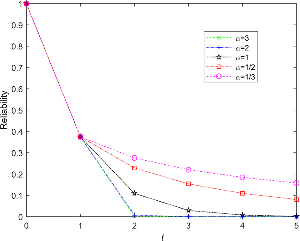


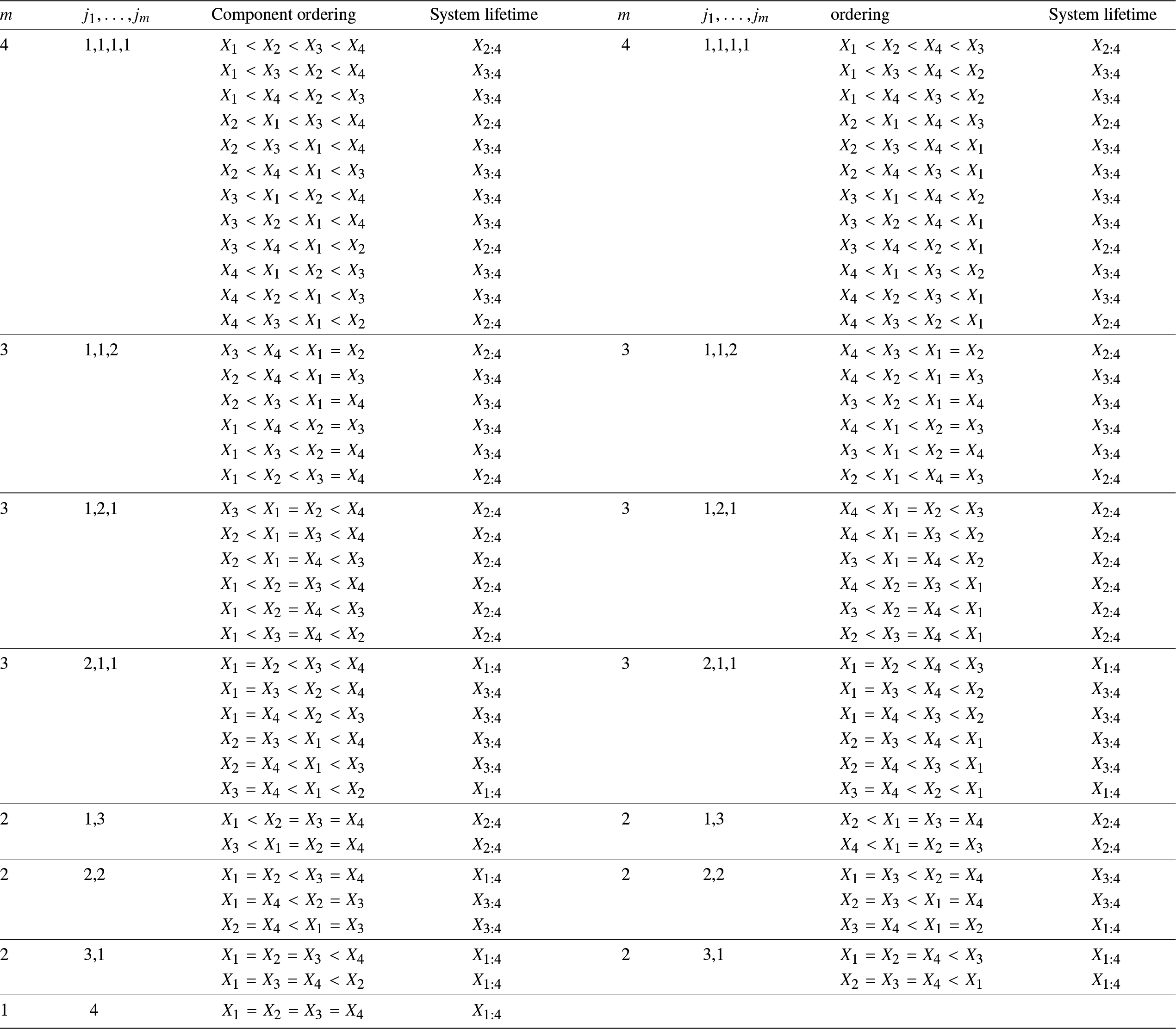


 Open access