


1. Introduction
Volvox, Marine Zooplankton, Paramecium, sperm cell, Escherichia coli, etc., are the low-Reynolds-number microswimmers. They do not require any external force or torque to swim in a fluid. While some use flagella and cilia, others modulate their body shape asymmetrically to move in the fluid. It has been found that the microorganisms are capable of using different swimming gaits to escape from the adverse environment (Hamel et al. Reference Hamel, Fisch, Combettes, Williams and Baroud2011). Some of them exhibit only translational motion (Lighthill Reference Lighthill1952; Blake Reference Blake1971), while the others swim in helical paths (Friedrich Reference Friedrich2008) having both translational as well as rotational movements. In general, microorganisms generate unsteady flows while swimming due to the sudden start from rest in a still medium. Planktonic organisms, which significantly affect trophic dynamics, are the most common examples of unsteady swimmers. Some of them exhibit oscillatory flows due to the synchronous movement of the appendage attached to the surface of the body (Klindt & Friedrich Reference Klindt and Friedrich2015). Guasto, Johnson & Gollub (Reference Guasto, Johnson and Gollub2010) have measured experimentally the time-dependent velocity field of C. reinhardtii. Unsteadiness can also occur for several other reasons, for example: (i) the unsteady beating of the appendages attached to the surface of the body; (ii) velocity fluctuations developed in the presence of the predator and prey; and (iii) turbulent ambient flow (Crawford & Purdie Reference Crawford and Purdie1992; Magar & Pedley Reference Magar and Pedley2005).
The time-dependent movement of a passive body has been well studied (Basset Reference Basset1888; Auton, Hunt & PruďHomme Reference Auton, Hunt and PruďHomme1988; Prakash & Raja Sekhar Reference Prakash and Raja Sekhar2012). However, the unsteady motion of microorganisms has not been explored much in the past. The squirmer model (Lighthill Reference Lighthill1952; Blake Reference Blake1971) was extended to study the unsteady motion of ciliated microorganisms by Rao (Reference Rao1988). Later, this model was extended by Ishimoto and others to study the motion of an unsteady inertial squirmer with a small surface deformation under the action of gravity (Ishimoto Reference Ishimoto2013). Recently, Magar and others used the squirmer model (Lighthill Reference Lighthill1952; Blake Reference Blake1971), which exploits time-dependent but quasi-steady flow fields around the body, to explain the nutrient uptake of the unsteady but inertia-free squirmer (Magar & Pedley Reference Magar and Pedley2005). Moreover, as an unsteady squirmer swims in a nutrient-enriched environment, its nutrient uptake rate increases with increasing speed (Magar & Pedley Reference Magar and Pedley2005). On the other hand, Wang & Ardekani (Reference Wang and Ardekani2012) studied the unsteady squirmer propelling in a non-uniform background flow. Notably, the biogenic mixing in the environment is aided by a collection of unsteady microswimmers (Thiffeault & Childress Reference Thiffeault and Childress2010; Lin, Thiffeault & Childress Reference Lin, Thiffeault and Childress2011; Mueller & Thiffeault Reference Mueller and Thiffeault2017). Unsteadiness also results in the microorganisms’ motion due to the entrapment of the body at the water–air interface, as observed experimentally for Tetrahymena (Ferracci et al. Reference Ferracci, Ueno, Tsuruta, Imai, Yamaguchi and Ishikawa2013). Note that the scallop theorem is invalid for unsteady squirmers if inertial effects are taken into account (Lauga Reference Lauga2007; Wang & Ardekani Reference Wang and Ardekani2012).
Not only geometric confinement but also external stimuli like light (Mitchell et al. Reference Mitchell, Alonso, Lalucat, Esteve and Brown1991) and chemical substances (Houten Reference Houten1978; Mitchell et al. Reference Mitchell, Alonso, Lalucat, Esteve and Brown1991) can change the swimming dynamics of a microorganism. In biological systems, though diffusion influences many transport phenomena, directed motion is also significant. The term taxis refers to the locomotion of a body in response to its environment. If the external stimulus is a chemical substance, then the microorganism's response by changing its course of motion is known as chemotaxis. If the microorganism gets attracted by the stimulus, then it is called positive chemotaxis, and if repelled, it is called negative chemotaxis (Tsang, Macnab & Koshland Reference Tsang, Macnab and Koshland1973). Both natural and artificial swimmers can exhibit chemotaxis (Paxton et al. Reference Paxton, Kistler, Olmeda, Sen, Angelo, Cao, Mallouk, Lammert and Crespi2004; Hong et al. Reference Hong, Blackman, Kopp, Sen and Velegol2007; Geiseler et al. Reference Geiseler, Hänggi, Marchesoni, Mulhern and Saveĺev2016; Jin, Üger & Maass Reference Jin, Üger and Maass2017). For example, artificial swimmers include Janus particles that are driven by self-thermophoresis created by laser irradiation (Jiang, Yoshinaga & Sano Reference Jiang, Yoshinaga and Sano2010), and nanorobots (Sengupta, Ibele & Sen Reference Sengupta, Ibele and Sen2012) can accelerate if subjected to external stimuli. Experimentally, it has been found that designed magnetic microswimmers can be used as an effective transport agent (Kokot et al. Reference Kokot, Kolmakov, Aranson and Snezhko2017) for drug delivery. Also, the confined motion of magnetic colloidal particles in the presence of a sinusoidal magnetic field is useful for designing microfluidic devices (Tierno et al. Reference Tierno, Golestanian, Pagonabarraga and Sagués2008). The time-dependent magnetic field can influence profoundly the translational-rotational coupling in the motion of the artificial swimmers, giving rise to different types of swimming paths, for example, helical and superhelical. Bio-inspired unsteady artificial swimmers have biomedical applications (Tabak & Yesilyurt Reference Tabak and Yesilyurt2012). Though the accelerated motion of microorganisms is energetically expensive, it is the only way out for them under the attack of a predator.
Moreover, in unsteady swimming while the dominating viscous force keeps the Reynolds number  $(Re = \rho U a/\eta )$ low, the unsteady inertia enters through the Strouhal number $(Sl)$. The Strouhal number is defined as $Sl = a/U\tau$. Here, $a/U$ is the convective time scale, and $\tau$ is the unsteady time scale. Consequently, $Sl\,Re$ measures the relative magnitude of unsteady inertia. Note that $a$ is the characteristic length scale of the body, $U$ is the characteristic velocity of the body, $\rho$ is the fluid density, and $\eta$ is the fluid viscosity. Thus for a higher $Sl$, the oscillation in the flow, i.e. unsteady inertia, dominates. Moreover, unsteady inertia dominates the hydrodynamic forces while the vorticity around the swimmer has not been diffused out to a large distance (Lovalenti & Brady Reference Lovalenti and Brady1993). Notably, the convective inertia is negligible in the previous case. We assume $Re \ll Sl$ in this work. The former assumptions work well for many microorganisms. For example, for an algal cell, $Re = 0.001$ and $Sl = 1$ (Guasto et al. Reference Guasto, Johnson and Gollub2010). The unsteady inertial forces acting on the unsteady swimmer use the terms Basset force and added mass force (Basset Reference Basset1888). The Basset or history force is due to the lagging boundary layer around the unsteady swimmer. On the other hand, the added mass force arises as the body accelerating in a medium generates an instantaneous pressure field in the surrounding medium. Hence not only the body but a portion of the medium accelerates with the body, giving rise to added mass effect. Therefore, it is crucial to understand unsteady bio-locomotion to gain better knowledge about various natural phenomena and biomedical applications involved with them.
In this article, we aim to study the hydrodynamic behaviour of an unsteady chiral swimmer (non-axisymmetric). We use the unsteady version of the generalized squirmer model called the chiral squirmer (Maity & Burada Reference Maity and Burada2019; Burada, Maity & Jülicher Reference Burada, Maity and Jülicher2021), a non-deformable spherical body that is free from external forces and torques. However, the swimmer experiences forces from its own generated flow field. We solve the corresponding unsteady Stokes equation with appropriate boundary conditions, using the double curl representation (Venkatalaxmi, Padmavathi & Amarnath Reference Venkatalaxmi, Padmavathi and Amarnath2004a). Note that the former method has been proved to provide a complete general solution to the unsteady Stokes equation (Venkatalaxmi, Padmavathi & Amarnath Reference Venkatalaxmi, Padmavathi and Amarnath2004b). We calculate the flow field, migration velocity and rotation rate of an unsteady chiral swimmer in a closed form. This migration velocity is compared with the known results in the axisymmetric limit. Later, we investigate numerically the response of the unsteady chiral swimmer to an external chemical stimulus.
The paper is organized as follows. In § 2, we introduce the unsteady chiral squirmer model. In § 3, we discuss the hydrodynamic flow fields of the swimmer. Section 4 provides the response of an unsteady swimmer to an external chemical gradient. The main conclusions are provided in § 5.
2. Unsteady chiral swimmer model
In general, when microswimmers swim in a fluid, the inertial effects can usually be neglected as they belong to the low-Reynolds-number regime. However, unsteady or oscillatory swimming may be important in many biological phenomena. The hydrodynamic flow field generated by a swimmer then obeys the unsteady Stokes equation (Happel & Brenner Reference Happel and Brenner1986)
 \begin{equation} \rho\,\frac{\partial \boldsymbol{v}}{\partial t} ={-} \boldsymbol{\nabla} p + \eta\,\nabla^2 \boldsymbol{v},\quad \boldsymbol{\nabla}\boldsymbol{\cdot} \boldsymbol{v} = 0, \end{equation}
where  $\boldsymbol {v}$ and $p$ are the velocity and pressure fields, respectively, and $\rho$ and $\eta$ are the density and viscosity of the surrounding fluid, respectively. The non-dimensionalization of (2.1a,b) is provided in Appendix A. There are minimal works in literature determining the general solution of the unsteady Stokes equation (Rao Reference Rao1988; Venkatalaxmi et al. Reference Venkatalaxmi, Padmavathi and Amarnath2004a). In this study, we have considered the solution by Venkatalaxmi et al. (Reference Venkatalaxmi, Padmavathi and Amarnath2004a) to determine the flow field around a chiral swimmer. The details are provided in Appendix B.
A chiral squirmer is a rigid spherical body of radius  $a$ with a tangential active surface slip. However, in the current study, the active slip $\boldsymbol{\mathcal{{V}}}_s (\theta, \phi, t)$ is time-dependent. It is parametrized by the polar and azimuthal angles $\theta$ and $\phi$, respectively, and defined in a body-fixed frame $(\boldsymbol {n}, \boldsymbol {b}, \boldsymbol {t})$ in terms of gradients of spherical harmonics that form a basis for tangential vectors on the surface. The general unsteady slip on the surface of the spherical body is prescribed as
 \begin{equation} \boldsymbol{\mathcal{{V}}}_s (\theta, \phi, t) = \boldsymbol{v}_s (\theta, \phi, t) + \boldsymbol{v}_s^d (\theta, \phi, t), \end{equation}
where,
 $$\begin{gather} \boldsymbol{v}_s (\theta, \phi, t) = \sum_{l=1}^\infty\,\sum_{m= 0}^l \sum_{j=0}^\infty [-\delta_{l m }^j \boldsymbol{\nabla}_s S_{l m}^j(\theta, \phi)+ \xi_{l m}^j \boldsymbol{e}_r \times \boldsymbol{\nabla}_s T_{l m}^j(\theta, \phi)] {\rm e}^{\lambda_j^2 t}, \end{gather}$$
 $$\begin{gather}\boldsymbol{v}_s^d (\theta, \phi, t) = \sum_{l=1}^\infty \sum_{m= 0}^l \sum_{k=1}^\infty [-\delta_{l m }^{\prime k} \boldsymbol{\nabla}_s S_{l m}^{\prime k}(\theta, \phi) + \xi_{l m}^{\prime k} \boldsymbol{e}_r \times \boldsymbol{\nabla}_s T_{l m}^{\prime k}(\theta, \phi)] {\rm e}^{\lambda_k^2 t}, \end{gather}$$
where  $\delta _{l m}^j$, $\xi _{l m}^j$, $\delta _{l m}^{\prime k}$ and $\xi _{l m}^{\prime k}$ are the slip coefficients; $\boldsymbol {\nabla }_s = \boldsymbol {e}_\theta ({\partial }/{\partial \theta }) + \boldsymbol {e}_ \phi ({1}/{\sin \theta }) ({\partial }/{\partial \phi })$ is the surface gradient operator; $S_{l m}^j(\theta, \phi )$ and $T_{l m}^j(\theta, \phi )$ are the spherical harmonics, having the form $S_{l m}^j(\theta, \phi ) = P_l^m(\cos \theta ) (A_{l m}^j \cos m\phi + B_{l m}^j \sin m\phi )$ and $T_{l m}^j(\theta, \phi ) = P_l^m(\cos \theta ) (C_{l m}^j \cos m\phi + D_{l m}^j \sin m\phi )$, respectively, where $P_l^m (\cos \theta )$ are the associated Legendre polynomials; and similarly, $S_{l m}^{\prime k}(\theta, \phi ) = P_l^m(\cos \theta ) (A_{l m}^{\prime k} \cos m\phi + B_{l m}^{\prime k} \sin m\phi )$ and $T_{l m}^{\prime k}(\theta, \phi ) = P_l^m(\cos \theta ) (C_{l m}^{\prime k} \cos m\phi + D_{l m}^{\prime k} \sin m\phi )$. Note that the slip velocity is decomposed into two parts, as the first corresponds to the oscillatory part and the second corresponds to the decaying part, consistent with the general solution of the unsteady Stokes equation. Also, while the first part of the slip velocity is essential to capture the long-time unsteady behaviour of the swimmer, the decaying part is necessary to capture the transient motion of the swimmer.
We use the above slip velocity and calculate the flow field generated by the unsteady chiral swimmer (see (B1)). In the flow field solution,  $\lambda ^2_{n}$ ( $n = j, k$) can be either complex or real. Therefore, to deal with the complete solution, we consider both $\lambda ^2_j = ij$ and $\lambda _k^2 = - k$. Here, ${\rm i} = \sqrt {-1}$. We can see that $\lambda _{j}^2$ is a constant related to the frequency of the body's oscillatory motion, while $\lambda _{k}^2$ belongs to its transient motion. Note that $j = k = 0$ corresponds to the steady part of the slip. However, to avoid repetition, we consider the case $k > 0$ in the current study. As in the case of a steady swimmer, while the first mode in the slip velocity ( $l = 1$) is related to the translational and rotational motion of the swimmer, the $l = 2$ mode corresponds to the leading-order flow field. Usually, the contribution of the higher-order modes ( $l > 2$) can be ignored. Thus for the rest of the paper, we include only $l = 1, 2$ modes in the surface slip. It may be noted that in the limit $\lambda _{j,k} \rightarrow 0$, by setting $\xi _{l m}^{j,\prime k} = 0$ in the surface slip (2.2), one can retrieve the simple axisymmetric squirmer model introduced by Lighthill (Reference Lighthill1952). However, in the same limit, by setting only $\xi _{l m}^{j, \prime k} \neq 0$, the chiral squirmer model can be retrieved (Burada et al. Reference Burada, Maity and Jülicher2021). Thus the surface slip (2.2) in the current model is very general. In the following, for simplicity, we consider only the first few oscillatory modes of the surface slip, i.e. $j = 0,1,2$ and $k = 1, 2$, and neglect higher-frequency modes. This time-dependent slip causes the swimmer to change its nature cyclically with time from puller to pusher, and vice versa (see figure 1). The nature of the swimmer can be captured through the parameter $\beta$ (see figure 1d), which is defined as
 \begin{equation} \beta = \frac{\sum_{m= 0}^2 \sum_{j=0}^2 \sum_{k=1}^2 \delta_{2\unicode{x2009}m }^{j, \prime k} \,{\rm e}^{\lambda_{j,k}^2 t} }{\sum_{m= 0}^1 \sum_{j=0}^2 \sum_{k=1}^2 \delta_{1\unicode{x2009}m }^{j, \prime k}\,{\rm e}^{\lambda_{j,k}^2 t}}. \end{equation}
Note that the former behaviour is common in many microorganisms (Klindt & Friedrich Reference Klindt and Friedrich2015; Wu et al. Reference Wu, Farutin, Hu, Thiébaud, Rafaï, Peyla, Lai and Misbah2016; Hintsche et al. Reference Hintsche, Waljor, Großmann, Kühn, Thormann, Peruani and Beta2017). However, a steady squirmer never changes its nature of swimming over time.
Real part of the three-dimensional flow field at the surface of an unsteady chiral swimmer at different dimensionless times  $t = 0$ (a), $t = 26$ (b), and $t = 28$ (c), plotted in the laboratory frame of reference. The swimmer propels with a time-dependent velocity $\boldsymbol {U}$ and rotation rate $\boldsymbol {\varOmega }$. $(\boldsymbol {n},\boldsymbol {b},\boldsymbol {t})$ is the frame attached to the swimmer at the centre of the body. The colour bar depicts the strength of the surface slip velocity. The parameter values are set to $\delta _{10}^{0\, A} = 2.39$, $\delta _{10}^{1\, A} = 1.72$, $\delta _{10}^{2\, A} = -0.001$, $\delta _{10}^{\prime 1\, A} = -3.1$, $\delta _{10}^{\prime 2\, A} = -0.35$, $\delta _{20}^{0\, A} = 0$, $\delta _{20}^{1\, A} = 5.457$, $\delta _{20}^{2\, A} = -2.353$, $\delta _{20}^{\prime 1\, A} = -5.457$, $\delta _{20}^{\prime 2 \, A} = -2.353$, $\xi _{20}^{0\, C} = 2$, $\xi _{20}^{1 \, C} = 2$, $\xi _{20}^{2\, C} = 3$, $\xi _{20}^{\prime 1\, C} = -2$, $\xi _{20}^{\prime 2\, C} = -3$. Note that $n = 1$, $m = 0,1$ modes of the rotational part of the flow field do not contribute to the flow field in the lab frame of reference. (d) The time-dependent stresslet ( $\beta$) has been plotted as a function of time ( $t$) depicting the changing nature of the swimmer with time. Here, $\beta >0$ is a puller, $\beta <0$ is a pusher, and $\beta =0$ is a neutral swimmer.

2.1. Velocity and rotation rate
The instantaneous surface velocity determines the swimming speed and rotation rate of the unsteady swimmer. Using the Lorentz reciprocal theorem (Kim & Karrila Reference Kim and Karrila1991) for the unsteady Stokes flow, we calculate the velocity and rotation rate of the swimmer. The general expressions are given by (see Appendix C)
 $$\begin{gather} \boldsymbol{U}(t) = \boldsymbol{U}_0 + \sum_{j=1}^{\infty} {\rm Re} [\boldsymbol{U}^j \, {\rm e}^{\lambda^2_j t}] + \sum_{k=1}^{\infty} {\rm Re} [\boldsymbol{U}^{\prime k} \, {\rm e}^{\lambda^2_k t}], \end{gather}$$
 $$\begin{gather}\boldsymbol{\varOmega}(t) = \boldsymbol{\varOmega}_0 + \sum_{j=1}^{\infty} {\rm Re} [\boldsymbol{\varOmega}^j \, {\rm e}^{\lambda^2_j t}] + \sum_{k=1}^{\infty} {\rm Re} [\boldsymbol{\varOmega}^{\prime k} \, {\rm e}^{\lambda^2_k t}], \end{gather}$$
where
 $$\begin{gather} \boldsymbol{U}_0 = \frac{2}{3} (\delta_{1 1}^{0A}\boldsymbol{n} + \delta_{1 1}^{0B}\boldsymbol{b} + \delta_{1 0}^{0 A}\boldsymbol{t}), \end{gather}$$
 $$\begin{gather}\boldsymbol{U}^{j, \prime k} = \frac{2}{3}\,\frac{1+ a \lambda_{j,k}}{1 + a \lambda_{j,k} + (a^2 \lambda_{j,k}^2/3)} (\delta_{1 1}^{j, \prime k \, A} \boldsymbol{n} + \delta_{1 1}^{j,\prime k \, B}\boldsymbol{b}+ \delta^{j,\prime k \, A}_{1 0}\boldsymbol{t}), \end{gather}$$
 $$\begin{gather}\boldsymbol{\varOmega}_0 = \frac{\xi_{1 1}^{0C}}{a} \boldsymbol{n} + \frac{\xi_{1 1}^{0D}}{a} \boldsymbol{b} + \frac{\xi^{0 C}_{1 0}}{a} \boldsymbol{t}, \end{gather}$$
 $$\begin{gather}\boldsymbol{\varOmega}^{j, \prime k} = \frac{\xi_{1 1}^{j,\prime k \, C}}{a} \boldsymbol{n} + \frac{\xi_{1 1}^{j,\prime k \, D}}{a} \boldsymbol{b} + \frac{\xi^{j,\prime k \, C}_{1 0}}{a} \boldsymbol{t}. \end{gather}$$
Here,  $\delta _{1 0}^{j,\prime k \, A} = \delta _{1 0}^{j,\prime k} \times A_{ 1 0}^{j,\prime k}$, $\xi _{1 0}^{j,\prime k \,C} = \xi _{1 0}^{j,\prime k} \times C_{ 1 0}^{j,\prime k}$, $\xi _{1 1}^{j,\prime k \, C} = \xi _{1 1}^{j,\prime k} \times C_{ 1 1}^{j,\prime k}$, $\xi _{1 1}^{j,\prime k \, D} = \xi _{1 1}^{j,\prime k}\times$ $D_{ 1 1}^{j,\prime k}$, and $A_{lm}^{j,\prime k}$, $B_{lm}^{j,\prime k}$, $C_{lm}^{j,\prime k}$ and $D_{lm}^{j,\prime k}$ are the coefficients of $S_{l m}^{j, \prime k}$ and $T_{l m}^{j, \prime k}$. For simplicity, in the following, we measure the lengths in units of $a$, time in units of $1/\omega$ (where $\omega$ is the frequency of oscillations), and pressure in units of $\eta U_0/ a$ (where $U_0$ is the magnitude of the steady part of the swimmer's velocity). In the rest of the paper, we set the parameters $\delta ^{0\, A}_{1 1} = \delta ^{0\, B}_{1 1} = \xi ^{0 \, D}_{1 1} = 0$ and $\delta ^{j, \prime k \, A}_{1 1} = \delta ^{j, \prime k \, B}_{1 1} = \xi ^{j,\prime k \, D}_{1 1} = 0$, for any $j$, in (2.8), (2.9), (2.10) and (2.11) such that the body translates along the $\boldsymbol {t}$ direction, i.e. $\boldsymbol {U}(t) = U_t \boldsymbol {t}$ (see figure 1) and having the rotation rate in the $\boldsymbol {nt}$-plane. By doing so, we can reduce the number of free parameters in the model without changing the qualitative behaviour of the chiral swimmer.
Figure 2(a) depicts the strength of velocity  $U(t)$ of the unsteady chiral swimmer as a function of time $t$. The velocity obtained in our calculations is similar to the one calculated by Wang & Ardekani (Reference Wang and Ardekani2012) (see figure 2a). Note that in the latter, $U(t)$ is calculated analytically by using the fundamental equation of motion of an unsteady low- $Re$ swimmer without determining the hydrodynamic flow field around the body. However, the determined $U(t)$ of the body (Wang & Ardekani Reference Wang and Ardekani2012) is a function of the product of the Strouhal and Reynolds numbers. Conversely, $U(t)$ determined in our case depends purely on the coefficients of the prescribed time-varying surface slip velocity of the swimmer. The $Sl\,Re$ value is completely absorbed into the slip coefficients in our case. Note that the qualitative behaviour of $U(t)$ is the same in both the approaches. However, the minor discrepancy in the results may be due to differences in the approaches or free parameters chosen in the respective models. Note that while the unsteady velocity counts the contribution of the added mass and the Basset force, the velocity in the quasi-steady limit considers only the hydrodynamic force (Blake Reference Blake1971; Magar & Pedley Reference Magar and Pedley2005).
(a) Dimensionless swimming velocity  $U$ of the unsteady chiral swimmer compared with the results of Wang & Ardekani (Reference Wang and Ardekani2012) and Blake (Reference Blake1971). All the corresponding parameters have the same values as in figure 1. The velocities by Blake ( $U_{quasi\text {-}steady}$) and Wang ( $U_{{Wang}}$) are plotted with $B_{10} = 2.39$, $B_{11} = 3.5$, $B_{12} = 0.16$ and $Sl\,Re = 10$ (Wang & Ardekani Reference Wang and Ardekani2012). (b) Rotation rate ( $\varOmega$) of the chiral swimmer plotted as a function of time with $\xi _{10}^{0\, C}= \xi _{11}^{0\, C} = 1$, $\xi _{10}^{1\, C}= \xi _{11}^{1\, C} = 1.5$, $\xi _{10}^{2\, C}=\xi _{11}^{2\, C} = 0.04$, $\xi _{10}^{\prime 1\, C}= \xi _{11}^{\prime 1\, C} = -0.5$, $\xi _{10}^{\prime 2\, C}= \xi _{11}^{\prime 2\, C} = -0.5$. Here, $\varOmega = \sqrt {\varOmega _n^2 + \varOmega _t^2}$, where $\varOmega _n$ and $\varOmega _t$ are the components of the rotation rate along the $\boldsymbol {n}$ and $\boldsymbol {t}$ axes, respectively.

Additionally, the body possess a time-dependent rotation rate that is plotted in figure 2(b). As mentioned before,  $\boldsymbol \varOmega (t)$ has components along the $\boldsymbol {t}$ and $\boldsymbol {n}$ axes only. The rotation rate is oscillatory, and the behaviour is determined by $\varOmega = \sqrt {\varOmega _n^2 + \varOmega _t^2}$. Due to this choice, the unsteady swimmer moves in a superhelical path because $\varOmega _n$ and $\varOmega _t$ are time-dependent. If they were time-independent, then we would observe a helical path. Note that the added mass and the Basset force do not influence the magnitude of $\boldsymbol {\varOmega }(t)$; see (2.10) and (2.11).
Solving the force and torque balance equations for the chiral swimmer, the equations of motion of the swimmer can be obtained, which are analogous to the Frenet–Serret equations. They read
 \begin{equation} \left.\begin{gathered} \dot{\boldsymbol{r}} = \boldsymbol{U}(t), \\ \dot{\boldsymbol{n}} = \boldsymbol{\varOmega}(t)\times \boldsymbol{n},\quad \dot{\boldsymbol{b}} = \boldsymbol{\varOmega}(t)\times \boldsymbol{b},\quad \dot{\boldsymbol{t}} = \boldsymbol{\varOmega}(t)\times \boldsymbol{t}. \end{gathered}\right\} \end{equation}
The swimming path, generated by (2.12), depends on the strengths of  $\boldsymbol {U}(t)$ and $\boldsymbol \varOmega (t)$, and the correlation between them. In the case of a steady chiral swimmer, the path is a helix (Burada et al. Reference Burada, Maity and Jülicher2021). However, in the present case, the resultant swimming path is not helical but superhelical or deformed helical (figure 5b). Notably, a similar superhelical path has been observed for flagellated microorganisms modelled with the three-sphere model (Cortese & Wan Reference Cortese and Wan2020).
3. Unsteady hydrodynamic flow
Figure 3 depicts the comparison of the axisymmetric part of the velocity field obtained for the current model with that of Blake and others (Blake Reference Blake1971; Magar & Pedley Reference Magar and Pedley2005) at times  $t = 0, 26$. The plots are in the laboratory frame of reference. Note that Blake's solution is obtained in the quasi-steady limit of the Stokes equation. We consider the first three terms of the time-dependent surface slip velocity given by Blake and others:
 $$\begin{gather} B_1 = B_{10} + B_{11}\cos \omega t + B_{12}\cos 2\omega t, \end{gather}$$
 $$\begin{gather}B_2 = B_{21}\sin \omega t + B_{22}\sin 2\omega t, \end{gather}$$
 $$\begin{gather}B_3 = B_{30} + B_{31}\cos \omega t + B_{32}\cos 2\omega t. \end{gather}$$
Here,  $\omega$ is the time-dependent surface squirming frequency. We assume that the former frequency is the same as the frequency of the oscillatory motion of the unsteady chiral squirmer. While the first index of $B_{nl}$ ( $n = 1,2,3$, $l = 0,1,2$) on the right-hand side of (3.1) implies the order of the mode amplitudes, the second index is related to harmonics of a fundamental frequency of oscillation. Also, in Blake's solution, the flow field is due to the force dipole or hydrodynamic stresslet (source dipole), while $B_2(t)\ne 0$ ( $B_2(t) = 0$), i.e. the field decays as $1/r^2$ ( $1/r^3$); see figures 3(e–h). Whereas, in our case, four strong vortices are formed in the vicinity of the swimmer due to the inertial effects, i.e. $Re_{osc} >0$. Here, $Re_{osc} = \rho \omega a^2/\eta$ is the oscillatory Reynolds number. Thus the flow field due to the oscillating stresslet ( $o(1/r^2)$) shows dominating quadrupolar symmetry; see figures 3(b,d). While the vortices near the body are stronger, they decay fast away from the swimmer. The complex vorticity field is a common feature of an unsteady swimmer (Li, Ostace & Ardekani Reference Li, Ostace and Ardekani2016) with the existence of a stagnation region. The stress exerted by the swimmer on the surrounding fluid causes the medium to strain. For an unsteady swimmer, the strain in the surrounding medium appears as vortices in the vicinity of the swimmer. Also, the flow field has stagnation points where the fluid velocity is zero, connected by a circle (see figure 3a). Similar behaviour can be observed in the velocity field obtained by Blake's solution, at $t = 15.6$ (not shown in the figure). Since the swimmer here is of an unsteady nature, the appearance of the stagnation boundary is time-dependent, present at $t=0$ but absent at $t= 26$ (see figures 3a,c). Note that the radius of the stagnation region changes randomly with both time $t$ and the parameter $\beta$.
Real part of the flow field around an axisymmetric swimmer in different planes at different times. Panels (a–d) show the flow fields of unsteady swimmer, in the absence of chirality, compared with those of a quasi-steady swimmer (Magar & Pedley Reference Magar and Pedley2005) (e–h). Here, the velocity profiles are projected onto the  $xy$-plane at $z = a$ (radius of the swimmer) and the $yz$-plane at $x = a$: (a,b,e, f) at $t = 0$, and (c,d,g,h) at $t = 26$. For the unsteady swimmer, parameters are used as in figure 1. For the quasi-steady swimmer, the parameters are $B_{10} = 2.39$, $B_{11} = 3.5$, $B_{12} = 0.16$, $B_{20}=0$, $B_{21} = 5.457$ and $B_{22} = -2.353$ (Magar & Pedley Reference Magar and Pedley2005; Wang & Ardekani Reference Wang and Ardekani2012). The stagnation regions are the common feature of unsteady swimmers, shown by a circle in (a). The colour bar indicates the strength of the velocity field.

Figures 4(a–d) depict the flow field of a chiral swimmer, i.e. considering the rotational part, at times  $t = 0$ and $26$. At $t = 0$, the generated flow pattern comprises a whirl in place of the stagnation contour at a distance from the surface of the chiral swimmer due to the rotational flow (see figure 4a). However, as observed in figure 3, after some time (e.g. $t = 26$), this whirl disappears (see figure 4c). Note that the vortices are anticlockwise (positive) for $t = 0$, and clockwise (negative) for $t = 26$ (see figures 4(b,d) and 3(b,d)). These vortices result from the flow field induced by the swimmer in earlier times. The direction of the vorticity depends on the nature of the swimmer (Chisholm et al. Reference Chisholm, Legendre, Lauga and Khair2016), i.e. puller or pusher, which oscillates with time.
Real part of the flow field around an unsteady chiral swimmer in different planes at different times:  $t = 0$ (a,b), and $t = 26$ (c,d). Here, the velocity profiles are projected onto the $xy$-plane at $z = a$ (radius of the swimmer) and the $yz$-plane at $x = a$. The parameters are used as in figure 1. The colour bar indicates the strength of the velocity field.

4. Response of an unsteady chiral swimmer to an external chemical gradient
In general, microorganisms respond to the external gradient (stimulus) present in the environment by swimming towards (Kirchman Reference Kirchman1994) or away from it. The directional movement of the self-propelled body in an external chemical stimulus is known as chemotaxis. Most of the ciliated microorganisms exhibit chemotaxis. For example, the ciliated microorganism Paramecium shows chemotactic behaviour with the help of receptors existing either on its ciliary membrane (Doughty Reference Doughty1979) or on the cell membrane of the organism (Oami Reference Oami1996). However, the detailed mechanism is not known. In chemotaxis, the ligands bind to the receptors on the body's surface, which triggers the internal signalling network of the body. This network modifies the velocity and rotation rate of the swimmer so that it can follow up the chemical gradient (Bohmer et al. Reference Bohmer, Van, Wayand, Hagen, Beyermann, Matsumoto, Hoshi, Hildebrand and Kaupp2005; Friedrich Reference Friedrich2008). Therefore, the body adapts to the chemical stimulus and responds or relaxes accordingly (Maity & Burada Reference Maity and Burada2019).
To understand the swimmer's adaptation and relaxation mechanism in the presence of a chemical gradient, we adopt the Barkai–Leibler model (Barkai & Leibler Reference Barkai and Leibler1997), which is a simple model for information processing and memory via the internal biochemical network. This model has been used widely for bacterial and sperm chemotaxis (Bohmer et al. Reference Bohmer, Van, Wayand, Hagen, Beyermann, Matsumoto, Hoshi, Hildebrand and Kaupp2005; Friedrich Reference Friedrich2008). The mechanism of adaptation and relaxation can be described by a simple dynamical system (Barkai & Leibler Reference Barkai and Leibler1997)
 $$\begin{gather} \sigma \dot{a_b} = p_b (S_b + S) - a_b, \end{gather}$$
 $$\begin{gather}\mu \dot{p_b} = p_b (1-a_b), \end{gather}$$
where  $\sigma$ is the relaxation time, $\mu$ is the adaptation time, $a_b(t)$ is the output variable that controls the velocity and rotation rate of the swimmer, $p_b (t)$ is the dynamic sensitivity, and $S_b(t)$ arises from the background activity in the absence of the ligand. The latter has a dimension of concentration. Note that these equations are applicable to weak concentration gradient limit only. Under a constant stimulus $S(t) = S_c$, the system reaches a steady state; the unsteady swimmer propels along a fixed direction, retaining its unperturbed swimming path. In the steady state, $a_b = 1$ and $p_b = 1/(S_b + S_c)$. As before, we scale $\mu$ and $\sigma$ with the oscillatory time scale $1/\omega$. For simplicity, we set the scaled values at $\mu = \sigma = 1$.
We assume that the chemotactic stimulus modifies the unsteady swimmer's slip coefficients (2.3) and (2.4), which are related to the velocity and the rotation rate of the body, in the following way:
 \begin{equation} X = X^{(0)} + X^{(1)}[a_b(t) - 1], \end{equation}
where  $X = (\delta _{l m}^{j, \prime k \, A}, \xi _{l m}^{j, \prime k \, C})$. Since the velocity and the rotation rate solely dictate the path of the body, it is sufficient to consider only the first mode in the slip velocity (2.2), i.e. we set $l = 1$. Note that all the $X^{0}$ terms are the unperturbed slip coefficients, i.e. in the absence of chemical gradient, whereas the terms with $X^{1}$ are the modified slip coefficients in the presence of the chemical gradient. Henceforth, the velocity and rotation rate of the body alter in a chemical gradient. Note that while there is no external chemical gradient, $a_b (t)$ attains its steady-state value, which is 1. Consequently, we can see that perturbation ( $X^{(1)}$) in the slip coefficients vanishes in the absence of chemical gradient; see (4.2). The former equation is analogous to the variation of the curvature ( $\kappa$) and torsion ( $\tau$) of a sperm cell's trajectory in a chemical field (Friedrich Reference Friedrich2008). Note that $\kappa = |\boldsymbol {\varOmega } \times \boldsymbol {U}|/|\boldsymbol {U}|^2$ and $\tau = |\boldsymbol {\varOmega } \boldsymbol {\cdot } \boldsymbol {U}|/|\boldsymbol {U}|^2$. Again, $\boldsymbol {U}$ and $\boldsymbol {\varOmega }$ are functions of the slip coefficients. Therefore, the modification of slip coefficients alters the dynamic parameters of the swimmer. Consequently, its swimming path changes.
4.1. Radial chemical gradient
We consider that the unsteady swimmer is subjected to a radial chemical field with the form
 \begin{equation} c(\boldsymbol{r}(t)) = \frac{c_r}{r(t)}, \end{equation}
where  $c_r$ is the constant that depends on the diffusivity of the ligands, i.e. the rate at which ligands are released from the chemical target, and $r(t)$ is the distance between the centre of mass position of the swimmer and the chemical source, given by $r(t) = \sqrt {x(t)^2 + y(t)^2 + z(t)^2}$ if the source is placed at the origin $(0,0,0)$. The chemotactic stimulus (Friedrich Reference Friedrich2008), i.e. the local chemical concentration over the receptors, reads $S(t)= c(\boldsymbol {r}(t))$.
Here, our main assumptions are: (i) the chemical concentration difference along the length of the body is irrelevant as the chemical signalling system receives a temporal stimulus; and (ii) the coefficients of the slip velocity are modified by the signalling system. Also, to have a minimal model, we can safely ignore the higher-order terms corresponding to the oscillatory and transient parts, i.e.  $j, k > 1$ in $\boldsymbol {U}(t)$ and $\boldsymbol {\varOmega }(t)$. Therefore, we are left with the parameters $\delta _{1 0}^{j,\prime k \, A(0)}$, $\xi _{1 0}^{j,\prime k \,C(0)}$, $\xi _{1 1}^{j,\prime k \, C(0)}$ for the unperturbed part, and $\delta _{1 0}^{j,\prime k \,A(1)}$, $\xi _{1 0}^{j, \prime k \, C(1)}$, $\xi _{1 1}^{j, \prime k \, C(1)}$ for the perturbed part, with $j = 0, 1$ and $k = 1$. The steady parts of the velocity $\boldsymbol {U_0}$ and the rotation rate $\boldsymbol {\varOmega _0}$ are kept constant (see (2.6) and (2.7)). The transient parts of the velocity ( $\boldsymbol {U}^{\prime 1}$) and rotation rate ( $\boldsymbol {\varOmega }^{\prime 1}$) of the swimmer decay very fast and may not play a significant role in the process of chemotaxis. Thus we can keep them constant as well. Further, we can assume that the velocity of the swimmer is only slightly perturbed by the chemical gradient (Friedrich Reference Friedrich2008). For example, the ratio of perturbed to unperturbed slip coefficients is $\delta _{1 0}^{j,\prime k \,A(1)}/\delta _{1 0}^{j,\prime k \, A(0)} \sim 0.1$. The former assumption is inspired by the chemotactic response of several natural microswimmers (Friedrich Reference Friedrich2008; Pankratova et al. Reference Pankratova, Kalyakulina, Krivonosov, Denisov, Taute and Zaburdaev2018; Salek et al. Reference Salek, Carrara, Fernandez, Guasto and Stocker2019). However, the rotation rate can be highly perturbed by the chemical gradient, i.e. when we apply a radial chemical gradient, thus we are considering $\xi _{1 m}^{j \, C(1)} /\xi _{1 m}^{j \,C(0)} \sim 10$ (for $m = 0,1$).
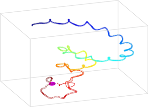
We solve (2.12) numerically, with the modified velocity and rotation rate of the swimmer in the presence of the chemical gradient to obtain the trajectory of the swimmer. Figure 5 depicts the chemotactic response of the swimmer for various strengths of the chemical gradient, where the source is placed at  $(0, 0, 0)$. For the steady case, the swimmers’ path is independent of $c_r$ (Maity & Burada Reference Maity and Burada2019). However, for the present case, the trajectory of the unsteady swimmer depends on the strength of $c_r$. Depending on the strength of the slip coefficients, the swimmer exhibits successful (S) chemotaxis (see figure 5a), unsuccessful (Un) chemotaxis (see figure 5b), and an interesting closed orbital state (O) near the chemical source (see figures 5c,d). In the case of successful chemotaxis, the swimmer moves in an irregular helical path; see figure 5(a). We have observed that the chemotactic success rate is irregular for the values of $c_r$ in the range $O(10^{-1})$, and beyond this range it is independent of $c_r$. Here, the swimmer's internal unsteadiness introduces the randomness in chemotactic navigation despite having a uniform gradient, giving rise to random motility or a persistent random walk. Therefore, $c_r$ is a useful determinant of chemotactic efficiency. On the other hand, the rotation rate can also dictate the success of the chemotaxis. For some values of the rotation rate, the chemical gradient cannot influence profoundly the body to steer towards the chemical source, leading to unsuccessful chemotaxis; see figure 5(b). Despite having a little influence on the dynamic parameters of the swimmer in the former case (see figures 6c, f), the gradient effectively reroutes the swimmer; see figure 5(b). Additionally, as the orientation of the rotation rate changes, the swimmer exhibits the interesting bounded state where it moves in a closed orbit around the source of the chemical gradient. The latter is a state between successful and unsuccessful chemotaxis. In this state, the chemical gradient is strong enough to trap a swimmer in an orbit but cannot influence it to reach the target. Thus the orbital state appears when there is a balance between the torque due to the radial chemical gradient and the torque generated by the swimmer. Note that the orbital state has been reported previously for artificial microswimmers (Takagi et al. Reference Takagi, Palacci, Braunschweig, Shelley and Zhang2014; Jin et al. Reference Jin, Vachier, Bandyopadhyay, Macharashvili and Maass2019).
Obtained numerically, the swimming paths of an unsteady chiral swimmer in a radial chemical gradient. The source (sphere) is at  $(0,0,0)$, and the swimmer's initial position is $(0, 20, 25)$. Lines and circles correspond to $c_r = 0.1$ and $c_r = 1$, respectively. The dotted line in (b) corresponds to the $c_r = 0$ or unperturbed state. Here, the adaptation and relaxation times are set to $\sigma = \mu = 1$, and the other parameters are set to $\delta _{10}^{0 \, A(0)} = 2.39$, $\delta _{10}^{0 \, A(1)} = \delta _{10}^{0 \, A(0)}/10$, $\delta _{10}^{\prime 1 \, A(0)} = -2.3$, $\delta _{10}^{\prime 1\, A(1)} = \delta _{10}^{\prime 1\, A(0)}/10$, $\delta _{10}^{1\, A(0)} = 1.4$, $\delta _{10}^{1\, A(1)} = \delta _{10}^{1\, A(0)}/10$, $\xi _{10}^{0 \, C(0)} = 0.2$, $\xi _{11}^{0\, C(0)} = 0.9$, $\xi _{10}^{0\, C(1)} = 2$, $\xi _{11}^{0\, C(1)} = -2$, $\xi _{10}^{\prime 1\, C(0)} = -0.5$, $\xi _{10}^{\prime 1\, C(1)} = -0.5$, $\xi _{10}^{1\, C(1)} = -10 \,|\xi _{10}^{1\, C(0)}|$, $\xi _{11}^{\prime 1 \, C(0)}= -0.5$, $\xi _{11}^{\prime 1\, C(1)} = -0.5$, $\xi _{11}^{1 \, C(1)} = 10 \, |\xi _{11}^{1\, C(0)}|$. For (a), $\xi _{10}^{1\, C(0)} =-2 \cos ({\rm \pi} /8)$, $\xi _{11}^{1\, C(0)}= 2 \sin ({\rm \pi} /8)$. For (b), $\xi _{10}^{1\, C(0)} =- \cos ({\rm \pi} /8)$, $\xi _{11}^{1\, C(0)}= \sin ({\rm \pi} /8)$. For (c,d), $\xi _{10}^{1\, C(0)} = -\cos (11{\rm \pi} /24)$, $\xi _{11}^{1 \, C(0)} = \sin (11{\rm \pi} /24)$. Panel (a) depicts the successful (S) chemotaxis, whereas (b) corresponds to the unsuccessful (Un) chemotaxis, and (c,d) show the trajectories corresponding to the orbital state (O). Panel (d) illustrates a closer view of the orbital state near the chemical target. The times along the swimming paths are encoded by colours shown in the colour bars.

Obtained numerically, the magnitudes of the velocity  $\boldsymbol {U}$ and rotation rate $\boldsymbol {\varOmega }$ are plotted as a function of time for various values of $c_r$. Panels (a,d) corresponds to successful chemotaxis; (b,e) belong to the orbital state; and (c, f) are associated with unsuccessful chemotaxis. All other parameters are the same as in figure 5.

Figure 6 shows the strengths of velocity  $\boldsymbol {U}(t)$ and rotation rate $\boldsymbol {\varOmega }(t)$ in the presence of the chemical gradient. Note that $U(t)$ of the swimmer is unchanged, whereas $\varOmega (t)$ varies irregularly. $\varOmega (t)$ diverges near the target in successful chemotaxis (see figure 6d) due to the saturation of the internal chemotactic network responsible for the relaxation and adaptation mechanism. However, the mildly affected velocity remains the same near the target; see figure 6(a). The degree of perturbation in $U(t)$ and $\varOmega (t)$ may be customized in an artificial swimmer; leading to different superhelical trajectories. In the orbital state, none of the dynamic parameters diverges as the swimmer never reaches the target; see figures 6(b,e). Yet, similar to successful chemotaxis, the variation in $\varOmega (t)$ varies irregularly over time while $U(t)$ varies periodically over time. Consequently, the gradient cannot strongly perturb the dynamic parameters in case of unsuccessful chemotaxis; see figures 6(c, f).
In the following, as the rotation rate plays a vital role in the chemotaxis of the chiral swimmer, we consider a situation where the strength of the chemical gradient is fixed ( $c_r = 1$), and vary the orientation ( $\chi$) and strength ( $H$) of the unperturbed oscillatory part of the rotation rate $\boldsymbol {\varOmega }^1$ systematically to understand the chemotactic behaviour of the unsteady swimmer by keeping the oscillatory part of the velocity $\boldsymbol {U}^1$ constant. Note that, as mentioned earlier, steady parts ( $\boldsymbol {U}_0,\boldsymbol {\varOmega }_0$) and decaying parts ( $\boldsymbol {U}^\prime,\boldsymbol {\varOmega }^\prime$) of the velocity and rotation rate are kept constant (see the caption of figure 5). We define the components of the unperturbed oscillatory part of the rotation rate $\boldsymbol {\varOmega }^{1(0)}$ as $\xi _{11}^{1\, C(0)}(\pm )= \pm H \sin (\chi )$, $\xi _{11}^{1\, D(0)}(\pm )= 0$, $\xi _{10}^{1\, C(0)}(\pm )= \pm H \cos (\chi )$, where $\chi$ is the angle between the swimming direction ( $\boldsymbol {t}$) and $\boldsymbol {\varOmega }^{1(0)}$, and the magnitude of $\boldsymbol {\varOmega }^{1(0)}$ is $H = \sqrt {(\xi _{11}^{1\, C(0)}(\pm ))^2 + (\xi _{10}^{1\, C(0)}(\pm ))^2}$. For example, $\xi _{11}^{1\, C(0)}(+)= + H \sin (\chi )$, $\xi _{10}^{1\, C(0)}(+) = + H \cos (\chi )$ are along the positive $\boldsymbol {n}$ and $\boldsymbol {t}$ axes, respectively. Similarly for the other combinations. Note that, as mentioned earlier, due to the external chemical gradient, the perturbed slip coefficients (4.2) of the rotational part vary as $\xi _{1 m}^{j \, C(1)} /\xi _{1 m}^{j \,C(0)} \sim 10$ (for $m = 0,1$).
Figure 7 depicts the swimming behaviour of an unsteady chiral swimmer in a radial chemical gradient for various orientations ( $\chi$) and strengths ( $H$) of the unperturbed oscillatory part of the rotation rate $\boldsymbol {\varOmega }^{1 (0)}$. The successful chemotaxis is observed mostly for $\boldsymbol {\varOmega }^{1(0)} = H (\sin \chi, 0, -\cos \chi )$ and $\boldsymbol {\varOmega }^{1(0)} = H (-\sin \chi, 0, -\cos \chi )$. In the other combinations, the orbital states appear. However, the unsuccessful state appear in all the combinations. For the case of a steady (time-independent) chiral swimmer, i.e. for $H = 0$, the chiral swimmer always exhibits successful chemotaxis (Maity & Burada Reference Maity and Burada2019). Due to the oscillatory nature of the swimmer, the swimming states show some retentiveness in the state diagrams (see figure 7). The time-dependent part in the rotation rate ( $\boldsymbol {\varOmega }^1$) introduces irregularity in the process of chemotaxis. As a result, higher magnitudes of $\boldsymbol {\varOmega }^1$, i.e. $H$, reduce the success rate of chemotaxis (see figure 7). The varying strength of the oscillatory part of the rotation rate does not always lead to successful chemotaxis. Therefore, only unsteady swimmers will successfully reach the chemical target, which will possess a specific rotation rate. For some combinations of $\chi$ and $H$, orbital states appear between the successful and unsuccessful states.
Obtained numerically, the state diagram depicting the swimming behaviour of an unsteady chiral swimmer in a radial chemical gradient for various orientations ( $\chi$) and strengths ( $H$) of the unperturbed oscillatory part of the rotation rate $\boldsymbol {\varOmega }^{1 (0)}$ (see the text for more details). The rest of the parameters are the same as those chosen in figure 5.

5. Conclusions
In this work, we have investigated an unsteady chiral swimmer's behaviour and its response to an external radial chemical gradient. We have prescribed a very general time-dependent slip velocity (non-axisymmetric) at the surface of the swimmer, and by using it, we have solved the unsteady Stokes equation for the velocity field. The corresponding time-dependent velocity and rotation rate of the swimmer are obtained using the Lorentz reciprocal theorem in a simple form. We showed that the unsteady inertial effects, due to added mass and Basset force, influence both the magnitude and the oscillatory behaviour of the velocity, whereas they can control only the oscillatory behaviour of the rotation rate. Thus the velocity of the unsteady swimmer differs from the quasi-steady swimmer. Also, an unsteady chiral swimmer produces vortices in the flow field. Indeed, the formation of vorticity causes a large amount of power dissipation. However, vortices may conceal mechanical strain fields that draw predators (Kiørboe Reference Kiørboe2011; Ergin Reference Ergin2015). Interestingly, due to time-dependent squirming, the swimmer oscillates between puller and pusher type.
In the absence of a chemical gradient, the unsteady chiral swimmer moves in a deformed helical path with varying speeds. However, when the swimmer is placed in a chemical gradient, its slip coefficients are modified, and correspondingly the velocity and rotation rates are altered. We have observed that the rotation rate plays a vital role in the response of the swimmer to a radial chemical gradient. The rotation rate leads to randomness in the swimming path, which essentially controls the success rate of the chemotaxis. The chemotactic movement of the swimmer is a stochastic function of the chemoattractant diffusivity ( $c_r$) in the range $o(10^{-1})$, and is independent of $c_r$ beyond that range.
This study is useful to understand the behaviour of unsteady ciliated microorganisms and their response to external gradients, e.g. chemical, temperature, etc. Also, it is helpful to design synthetic self-propelled bodies that can perform bio-mixing. Note that in the case of chemically active phoretic particles, the effective slip velocity at the surface of the swimmer is due to the diffusiophoresis process (Anderson Reference Anderson1989; Saha, Golestanian & Ramaswamy Reference Saha, Golestanian and Ramaswamy2014; Reigh et al. Reference Reigh, Chuphal, Thakur and Kapral2018). These artificial swimmers can sense the external chemical gradients by altering the slip velocity, and exhibit the chemotaxis. This process is analogous to what we have used in the current paper. However, the way slip velocity alters in phoretic particles is different from the present case.
Acknowledgments
The authors are grateful for insightful discussions with G.P. Raja Sekhar.
Funding
This work was supported by the Indian Institute of Technology Kharagpur, India.
Declaration of interests
The authors report no conflict of interest.
Appendix A. The non-dimensionalization of the unsteady Stokes equation
The Navier–Stokes equation is given by
 \begin{equation} \rho \left(
\frac{\partial \boldsymbol{v}}{\partial t} + \boldsymbol{v}
\boldsymbol{\cdot}\boldsymbol{\nabla} \boldsymbol{v}\right)
= \eta\,\nabla^2 \boldsymbol{v} - \boldsymbol{\nabla} p.\end{equation}
\begin{equation} \rho \left(
\frac{\partial \boldsymbol{v}}{\partial t} + \boldsymbol{v}
\boldsymbol{\cdot}\boldsymbol{\nabla} \boldsymbol{v}\right)
= \eta\,\nabla^2 \boldsymbol{v} - \boldsymbol{\nabla} p.\end{equation}
Here,  $\boldsymbol{v}$ denotes the unsteady flow field, $p$ denotes pressure, $\eta$ denotes viscosity, and $\rho$ denotes density of the fluid. Also, the radius of the spherical body, $a$, is the length scale, $1/\omega$ is the time scale, and $\eta U_0 /a$ is the pressure scale of the system. Furthermore, the velocity is scaled as $U_0$ (steady part of the swimmer's velocity). Thus we have two natural dimensionless numbers, $Re_{trans}$ (translational Reynolds number) and $Re_{osc}$ (oscillatory Reynolds number), defined as
 $$\begin{gather} Re_{trans} = \frac{\rho U_0 a}{\eta}, \end{gather}$$
 $$\begin{gather}Re_{osc} = \frac{\rho \omega a^2}{\eta}. \end{gather}$$
Using the above scales, the Navier–Stokes equation can be non-dimensionalized as
 \begin{equation}
Re_{osc}\,\frac{\partial \boldsymbol{\tilde{v}}}{\partial
\tilde{t}} + Re_{trans}\,\boldsymbol{\tilde{v}}
\boldsymbol{\cdot} \tilde{\boldsymbol{\nabla}}
\boldsymbol{\tilde{v}} = \tilde{\nabla}^2
\boldsymbol{\tilde{v}} - \tilde{\boldsymbol{\nabla}}
\tilde{p}. \end{equation}
\begin{equation}
Re_{osc}\,\frac{\partial \boldsymbol{\tilde{v}}}{\partial
\tilde{t}} + Re_{trans}\,\boldsymbol{\tilde{v}}
\boldsymbol{\cdot} \tilde{\boldsymbol{\nabla}}
\boldsymbol{\tilde{v}} = \tilde{\nabla}^2
\boldsymbol{\tilde{v}} - \tilde{\boldsymbol{\nabla}}
\tilde{p}. \end{equation}
In the limit  $Re_{osc} \gg Re_{trans}$, the second term on the left-hand side vanishes. The Strouhal number $Sl$ is defined as
 \begin{equation} Sl = \frac{a \omega}{U_0}. \end{equation}
Also,  $Re_{osc}$ can be expressed as $Re_{osc} = Re_{trans}\,Sl$. Therefore, the momentum equation reduces to the unsteady Stokes equation
 \begin{equation}
Sl\,Re_{trans}\,\frac{\partial
\boldsymbol{\tilde{v}}}{\partial \tilde{t}} =
\tilde{\nabla}^2 \boldsymbol{\tilde{v}} -
\tilde{\boldsymbol{\nabla}} \tilde{p}.
\end{equation}
\begin{equation}
Sl\,Re_{trans}\,\frac{\partial
\boldsymbol{\tilde{v}}}{\partial \tilde{t}} =
\tilde{\nabla}^2 \boldsymbol{\tilde{v}} -
\tilde{\boldsymbol{\nabla}} \tilde{p}.
\end{equation}
The unsteady Stokes equation is scaled as  $Sl \,Re$ (here, $Re = Re_{trans}$). In our study, the velocity of the swimmer is determined from the slip velocity of the body with the aid of the Lorentz reciprocal theorem. Clearly, $Sl\,Re$ is absorbed into the slip coefficients or coefficients of the velocity field. Therefore, we do not write $Sl\,Re$ explicitly in the general solution of the flow field. We drop the tildes afterwards for better readability.
Appendix B. Velocity field of an unsteady chiral swimmer
We calculate the velocity field of an unsteady chiral swimmer moving in a stagnant fluid. To do that, we start with the general solution of the unsteady Stokes equation (2.1a,b), which is given by (Venkatalaxmi et al. Reference Venkatalaxmi, Padmavathi and Amarnath2004a)
 \begin{equation} \boldsymbol{v} = \sum^\infty_{l=1} \sum^l_{m=0} \sum^\infty_{n = 0} (v_r \boldsymbol{e}_r + v_\theta \boldsymbol{e}_\theta + v_\phi \boldsymbol{e}_\phi ){\rm e}^{\lambda_n^2\nu t}, \end{equation}
where the components are
 \begin{gather} v_r = l(l+1) \left[{\mathcal{K}}^{n1}_{l m} r^{l-1} + \frac{{\mathcal{K}}^{n2}_{l m}}{r^{l+2}} + {\mathcal{K}}^{n3}_{l m}\, \frac{g_l(r\lambda_n)}{r} \right]S_{l m}^n(\theta, \phi), \end{gather}
 \begin{gather} v_\theta = \left[ (l+1) {\mathcal{K}}^{n1}_{l m} r^{l-1} - \frac{l {\mathcal{K}}^{n2}_{l m}}{r^{l+2}}+ {\mathcal{K}}^{n3}_{l m} \left((l+1)\, \frac{g_l(r\lambda_n )}{r}- \lambda_n\,g_{l+1}(r\lambda_n)\right)\right] \frac{\partial S_{l m}^n(\theta, \phi)}{\partial \theta} \nonumber\\ \hspace{-10.5pc} + \left[\frac{{\mathcal{K}}^{n4}_{l m}\,f_l(r\lambda_n) + {\mathcal{K}}^{n5}_{l m}\,g_l(r\lambda_n )}{\sin\theta}\right] \frac{\partial T_{l m}^n(\theta, \phi)}{\partial \phi}, \end{gather}
 \begin{gather} v_\phi = \frac{1}{\sin\theta} \left[ (l+1) {\mathcal{K}}^{n1}_{l m} r^{l-1} - \frac{l {\mathcal{K}}^{n2}_{l m}}{r^{l+2}}\,{\mathcal{K}}^{n3}_{l m} \left((l+1)\,\frac{g_l(r\lambda_n)}{r} - \lambda_n\, g_{l+1}(r\lambda_n)\right) \right] \frac{\partial S_{l m}^n(\theta, \phi)}{\partial \phi} \nonumber\\ \hspace{-11.5pc}-\left[\frac{{\mathcal{K}}^{n4}_{l m}\,f_l(r\lambda_n) + {\mathcal{K}}^{n5}_{l m}\,g_l(r\lambda_n)}{\sin\theta} \right] \frac{\partial T_{l m}^n(\theta, \phi)}{\partial \theta}. \end{gather}
Here,  $g_l(r \lambda _n) = \sqrt {{\rm \pi} /(2r \lambda _n)}\,K_{l+{1}/{2}}$ and $f_l(r \lambda _n) = \sqrt {{\rm \pi} /(2r \lambda _n)}\,I_{l+{1}/{2}}$ are the modified spherical Bessel functions of fractional order, and $S_{l m}^n(\theta, \phi )$ and $T_{l m}^n(\theta, \phi )$ are the spherical harmonics defined in § 2. The corresponding oscillatory pressure field is given by
 \begin{equation} p = p_0 - \sum^\infty_{l=1}\sum^l_{m=0}\sum^\infty_{n = 0}\lambda^2 \left[(l+1) {\mathcal{K}}^{n1}_{l m} r^l - {\mathcal{K}}^{n2}_{l m}\, \frac{l}{r^{l+1}}\right]S_{l m}^n(\theta, \phi)\,{\rm e}^{\lambda_n^2\nu t}. \end{equation}
 The boundary conditions at the surface of the chiral swimmer (at  $r = a$) are prescribed by the surface slip (2.2). However, in the far field, by setting $\boldsymbol {v}_{r \to \infty } = 0$, i.e. solving the velocity field in the laboratory frame of reference for the $l = 1$ mode, we get
 $$\begin{gather} {\mathcal{K}}_{1 m}^{n1} ={-}\frac{U_n}{2}, \end{gather}$$
 $$\begin{gather}{\mathcal{K}}_{1 m}^{n2} ={-}a^3\,\frac{-2\delta_{1m}^n\,g_1(\lambda_n a) + \lambda_n a\,g_2(\lambda_n a)\,U_n}{2(3\,g_1(\lambda_n a)- \lambda_n a\,g_2(\lambda_n a))}, \end{gather}$$
 $$\begin{gather}{\mathcal{K}}_{1 m}^{n3} = a\,\frac{-2\delta_{1m}^n + 3U_n}{2(3\,g_1(\lambda_n a)-\lambda_n a\,g_2(\lambda_n a))}, \end{gather}$$
 $$\begin{gather}{\mathcal{K}}_{1 m}^{n4} = 0, \end{gather}$$
 $$\begin{gather}{\mathcal{K}}_{1 m}^{n5} = \frac{\varOmega_n a - \xi_{1m}^n}{g_1(\lambda_n a)}. \end{gather}$$
 For  $l > 1$ modes,
 $$\begin{gather} {\mathcal{K}}_{l m}^{n1} = 0, \end{gather}$$
 $$\begin{gather}{\mathcal{K}}_{l m}^{n2} ={-} \frac{a^{l+2}\delta_{lm}^n\,g_l(\lambda_na )}{-g_l (\lambda_na)-2l\,g_l(\lambda_na)+\lambda_na\,g_{l+1}(\lambda_na)}, \end{gather}$$
 $$\begin{gather}{\mathcal{K}}_{l m}^{n3} = \frac{a\delta_{lm}^n}{-g_l(\lambda_na)-2l\,g_l(\lambda_na)+ \lambda_na\,g_{l+1}(\lambda_na)}, \end{gather}$$
 $$\begin{gather}{\mathcal{K}}_{l m}^{n4} = 0, \end{gather}$$
 $$\begin{gather}{\mathcal{K}}_{l m}^{n5} ={-}\frac{\xi_{lm}^n}{g_l(\lambda_na)}. \end{gather}$$
Note that  $\lambda _n^2 = \textrm {i} n \omega /\nu$ stands for oscillatory flow, while $\lambda _n^2 = - n \omega /\nu$ for transient decaying flow in general. However, in dimensionless units, as presented in § 2, $\lambda _n^2 = \textrm {i} n$ and $\lambda _n^2 = - n$ correspond to the oscillatory and decaying parts of the solution. In figure 3, we have plotted the real part of the general velocity field given above. In the main text, $n = j$ ( $\lambda _j^2 = \textrm {i} j$) corresponds to the flow's oscillatory part, and $n = k$ ( $\lambda _k^2 = -k$) corresponds to the transient decaying part of the flow. Accordingly, we have denoted the slip coefficients and the spherical harmonics without primes for the oscillatory part and with primes for the decaying part.
Appendix C. Derivation of the velocity and rotation rate of the unsteady swimmer from the Lorentz reciprocal theorem
Let  $\boldsymbol {v}_1$ and $\boldsymbol {v}_2$ both satisfy the unsteady Stokes equation. The corresponding stress tensors are $\boldsymbol {\sigma }_1$ and $\boldsymbol {\sigma }_2$, respectively. Notably, $\boldsymbol {\nabla } \boldsymbol {\cdot } \boldsymbol {\sigma }_i = \partial \boldsymbol {v}_i/\partial t$, with $i = 1,2$. We know that (Kim & Karrila Reference Kim and Karrila1991)
 \begin{equation} \boldsymbol{v}_1 \boldsymbol{\cdot} (\boldsymbol{\nabla} \boldsymbol{\cdot} \boldsymbol{\sigma}_2) - \boldsymbol{v}_2 \boldsymbol{\cdot} (\boldsymbol{\nabla} \boldsymbol{\cdot} \boldsymbol{\sigma}_1) = \boldsymbol{\nabla}\boldsymbol{\cdot} (\boldsymbol{v}_1 \boldsymbol{\cdot} \boldsymbol{\sigma}_2 - \boldsymbol{v}_2 \boldsymbol{\cdot} \boldsymbol{\sigma}_1). \end{equation}
By integrating over the volume  $V$ on both sides in this equation, and then using the Gauss divergence theorem on the right-hand side, we can obtain the Lorentz reciprocal theorem (Kim & Karrila Reference Kim and Karrila1991):
 \begin{gather} \unicode{x2232}_S \boldsymbol{v}_1 \boldsymbol{\cdot} (\boldsymbol{\sigma}_2 \boldsymbol{\cdot} \boldsymbol{n})\,{\rm d} S - \int_V \boldsymbol{v}_1 \boldsymbol{\cdot} (\boldsymbol{\nabla} \boldsymbol{\cdot} \boldsymbol{\sigma}_2) \,{\rm d} V= \unicode{x2232}_S \boldsymbol{v}_2 \boldsymbol{\cdot} (\boldsymbol{\sigma}_1 \boldsymbol{\cdot} \boldsymbol{n})\,{\rm d} S - \int_V \boldsymbol{v}_2 \boldsymbol{\cdot} (\boldsymbol{\nabla} \boldsymbol{\cdot} \boldsymbol{\sigma}_1)\,{\rm d} V. \end{gather}
Assuming similar time-dependency of both the solutions, we can write  $\boldsymbol {v}_i = \boldsymbol {v}_i(r,\theta, \phi )\,\textrm {e}^{\lambda ^2 \nu t}$ (Venkatalaxmi et al. Reference Venkatalaxmi, Padmavathi and Amarnath2004a) with $i=1,2$. Thus (C2) reduces to
 \begin{equation} \unicode{x2232}_S \boldsymbol{v}_1 \boldsymbol{\cdot} (\boldsymbol{\sigma}_2 \boldsymbol{\cdot} \boldsymbol{n})\,{\rm d} S = \unicode{x2232}_S \boldsymbol{v}_2 \boldsymbol{\cdot} (\boldsymbol{\sigma}_1 \boldsymbol{\cdot} \boldsymbol{n})\,{\rm d} S. \end{equation}
The solution  $(\boldsymbol {v}_1, \boldsymbol {\sigma }_1)$ is due to a force-free and torque-free unsteady swimmer. On the other hand, $(\boldsymbol {v}_2, \boldsymbol {\sigma }_2)$ is a solution due to a identical passive body subjected to a force $(\boldsymbol {F}_2)$ and torque $(\boldsymbol {T}_2)$ (Venkatalaxmi et al. Reference Venkatalaxmi, Padmavathi and Amarnath2004a). Thus we can write (Stone & Samuel Reference Stone and Samuel1996)
 $$\begin{gather} \boldsymbol{F}_2 \boldsymbol{\cdot} \boldsymbol{U}(t) ={-} \int_{S} \boldsymbol{n}\boldsymbol{\cdot} \boldsymbol{\sigma}_2\boldsymbol{\cdot} \boldsymbol{\mathcal{{V}}}_s \,{\rm d} S, \end{gather}$$
 $$\begin{gather}\boldsymbol{T}_2 \boldsymbol{\cdot} \boldsymbol{\varOmega}(t) ={-} \int_{S} \boldsymbol{n}\boldsymbol{\cdot} \boldsymbol{\sigma}_2\cdot \boldsymbol{\mathcal{{V}}}_s \,{\rm d} S. \end{gather}$$
For an unsteady swimmer moving with translational velocity  $\boldsymbol {U}(t)$ and rotation rate $\boldsymbol {\varOmega }(t)$, the flow field on its surface is $\boldsymbol {v}_1(a) = \boldsymbol {U}(t)+ \boldsymbol {\varOmega }(t) \times (a \boldsymbol {e}_r)+ \boldsymbol{\mathcal{{V}}}_s(\theta, \phi, t)$. Here, $\boldsymbol {e}_r$ is the unit outward normal on the surface of the swimmer, and $a$ is its radius. Also, $\boldsymbol{\mathcal{{V}}}_s$ is the time-dependent surface slip velocity; see § 2. Hence the velocity and rotation rate are
 $$\begin{gather} \boldsymbol{U}(t) = \boldsymbol{U}_0 + \sum_{j=1}^{\infty} {\rm Re} [\boldsymbol{U}^j \,{\rm e}^{\lambda^2_j \nu t} ] + \sum_{k=1}^{\infty} {\rm Re} [ \boldsymbol{U}^{\prime k} \, {\rm e}^{\lambda^2_k \nu t} ], \end{gather}$$
 $$\begin{gather}\boldsymbol{\varOmega}(t) = \boldsymbol{\varOmega}_0 + \sum_{j=1}^{\infty} {\rm Re} [\boldsymbol{\varOmega}^j \, {\rm e}^{\lambda^2_j \nu t} ] + \sum_{k=1}^{\infty} {\rm Re} [ \boldsymbol{\varOmega}^{\prime k} \, {\rm e}^{\lambda^2_k \nu t} ], \end{gather}$$
where the first term on the right-hand side corresponds to the steady (time-independent) migration velocity, the second term is related to the oscillatory part of the velocity, and the third term is related to the transient (decaying) part of the velocity. Here,
 $$\begin{gather} \boldsymbol{U}_0 = \frac{2}{3} (\delta_{1 1}^{0A}\boldsymbol{n} + \delta_{1 1}^{0B} \boldsymbol{b} + \delta_{1 0}^{0 A}\boldsymbol{t}), \end{gather}$$
 $$\begin{gather}\boldsymbol{U}^{j, \prime k} = \frac{2}{3}\, \frac{1+ a \lambda_{j,k}}{1 + a \lambda_{j,k} + (a^2 \lambda_{j,k}^2/3)} (\delta_{1 1}^{j, \prime k \, A} \boldsymbol{n} + \delta_{1 1}^{j,\prime k \, B} \boldsymbol{b}+ \delta^{j,\prime k \, A}_{1 0}\boldsymbol{t}), \end{gather}$$
 $$\begin{gather}\boldsymbol{\varOmega}_0 = \frac{\xi_{1 1}^{0C}}{a}\,\boldsymbol{n} + \frac{\xi_{1 1}^{0D}}{a}\,\boldsymbol{b} + \frac{\xi^{0 C}_{1 0}}{a}\,\boldsymbol{t}, \end{gather}$$
 $$\begin{gather}\boldsymbol{\varOmega}^{j, \prime k} = \frac{\xi_{1 1}^{j,\prime k \, C}}{a}\, \boldsymbol{n} + \frac{\xi_{1 1}^{j,\prime k \, D}}{a}\,\boldsymbol{b} + \frac{\xi^{j,\prime k \, C}_{1 0}}{a}\,\boldsymbol{t}. \end{gather}$$
The symbols have been discussed in § 2. As the Basset (history) and added mass forces act on the unsteady swimmer, the force-free condition contains the active force, hydrodynamic drag force and unsteady inertial force. Furthermore, the effective velocity of the body, (C8) and (C9), considers all the former forces. Thus the first equation of (2.12) can be found. Since the unsteady inertia does not influence the rotation rate of the swimmer (see (C10) and (C11)), the torque-free condition consists of active torque and hydrodynamic torque acting on the swimmer. Consequently, we can determine the remaining three equations of (2.12) (Kim & Karrila Reference Kim and Karrila1991).


 Open access