

1. Introduction
The free-electron laser (FEL) FLASH at DESY, Hamburg, Germany was the first vacuum ultraviolet (VUV) to soft x-ray FEL worldwide, starting with regular user operation in 2005[1]. FLASH is piloting many novel experiments and experimental techniques making use of these unique high-brilliance femtosecond-scale x-ray pulses. A list of publications on science at FLASH may be found in Ref. [2].
FLASH emerged from the TESLA Test Facility (TTF), a test bed for superconducting accelerating technology[Reference Edwards3]. In the framework of TTF, a prototype FEL has been set-up providing VUV radiation to piloting user experiments[Reference Andruszkow, Aune, Ayvazyan, Baboi, Bakker, Balakin, Barni, Bazhan, Bernard, Bosotti, Bourdon, Brefeld, Brinkmann, Buhler, Carneiro, Castellano, Castro, Catani, Chel, Cho, Choroba, Colby, Decking, Den Hartog, Desmons, Dohlus, Edwards, Edwards, Faatz, Feldhaus, Ferrario, Fitch, Flöttmann, Fouaidy, Gamp, Garvey, Gerth, Geitz, Gluskin, Gretchko, Hahn, Hartung, Hubert, Hüning, Ischebek, Jablonka, Joly, Juillard, Junquera, Jurkiewicz, Kabel, Kahl, Kaiser, Kamps, Katelev, Kirchgessner, Körfer, Kravchuk, Kreps, Krzywinski, Lokajczyk, Lange, Leblond, Leenen, Lesrel, Liepe, Liero, Limberg, Lorenz, Hua, Hai, Magne, Maslov, Materlik, Matheisen, Menzel, Michelato, Möller, Mosnier, Müller, Napoly, Novokhatski, Omeich, Padamsee, Pagani, Peters, Petersen, Pierini, Pflüger, Piot, Phung Ngoc, Plucinski, Proch, Rehlich, Reiche, Reschke, Reyzl, Rosenzweig, Rossbach, Roth, Saldin, Sandner, Sanok, Schlarb, Schmidt, Schmüser, Schneider, Schneidmiller, Schreiber, Schreiber, Schütt, Sekutowicz, Serafini, Sertore, Setzer, Simrock, Sonntag, Sparr, Stephan, Sytchev, Tazzari, Tazzioli, Tigner, Timm, Tonutti, Trakhtenberg, Treusch, Trines, Verzilov, Vielitz, Vogel, Walter, Wanzenberg, Weiland, Weise, Weisend, Wendt, Werner, White, Will, Wolff, Yurkov, Zapfe, Zhogolev and Zhou4–Reference Ayvazyan, Baboi, Bohnet, Brinkmann, Castellano, Castro, Catani, Choroba, Cianchi, Dohlus, Edwards, Faatz, Fateev, Feldhaus, Flöttmann, Gamp, Garvey, Genz, Gerth, Gretchko, Grigoryan, Hahn, Hessler, Honkavaara, Hüning, Ischebeck, Jablonka, Kamps, Körfer, Krassilnikov, Krzywinski, Liepe, Liero, Limberg, Loos, Luong, Magne, Menzel, Michelato, Minty, Müller, Nölle, Novokhatski, Pagani, Peters, Pflüger, Piot, Plucinski, Rehlich, Reyzl, Richter, Rossbach, Saldin, Sandner, Schlarb, Schmidt, Schmüser, Schneider, Schneidmiller, Schreiber, Schreiber, Sertore, Setzer, Simrock, Sobierajski, Sonntag, Steeg, Stephan, Sytchev, Tiedtke, Tonutti, Treusch, Trines, Türke, Verzilov, Wanzenberg, Weiland, Weise, Wendt, Wilhein, Will, Wittenburg, Wolff, Yurkov and Zapfe6]. First lasing was achieved in February 2000 at a wavelength of 109 nm[Reference Andruszkow, Aune, Ayvazyan, Baboi, Bakker, Balakin, Barni, Bazhan, Bernard, Bosotti, Bourdon, Brefeld, Brinkmann, Buhler, Carneiro, Castellano, Castro, Catani, Chel, Cho, Choroba, Colby, Decking, Den Hartog, Desmons, Dohlus, Edwards, Edwards, Faatz, Feldhaus, Ferrario, Fitch, Flöttmann, Fouaidy, Gamp, Garvey, Gerth, Geitz, Gluskin, Gretchko, Hahn, Hartung, Hubert, Hüning, Ischebek, Jablonka, Joly, Juillard, Junquera, Jurkiewicz, Kabel, Kahl, Kaiser, Kamps, Katelev, Kirchgessner, Körfer, Kravchuk, Kreps, Krzywinski, Lokajczyk, Lange, Leblond, Leenen, Lesrel, Liepe, Liero, Limberg, Lorenz, Hua, Hai, Magne, Maslov, Materlik, Matheisen, Menzel, Michelato, Möller, Mosnier, Müller, Napoly, Novokhatski, Omeich, Padamsee, Pagani, Peters, Petersen, Pierini, Pflüger, Piot, Phung Ngoc, Plucinski, Proch, Rehlich, Reiche, Reschke, Reyzl, Rosenzweig, Rossbach, Roth, Saldin, Sandner, Sanok, Schlarb, Schmidt, Schmüser, Schneider, Schneidmiller, Schreiber, Schreiber, Schütt, Sekutowicz, Serafini, Sertore, Setzer, Simrock, Sonntag, Sparr, Stephan, Sytchev, Tazzari, Tazzioli, Tigner, Timm, Tonutti, Trakhtenberg, Treusch, Trines, Verzilov, Vielitz, Vogel, Walter, Wanzenberg, Weiland, Weise, Weisend, Wendt, Werner, White, Will, Wolff, Yurkov, Zapfe, Zhogolev and Zhou4]. This was well beyond optical wavelengths, and at this time a world record toward shorter wavelength FELs.
With a major reconstruction finished in 2003, the TTF facility has been transformed into a FEL user facility named FLASH[Reference Ayvazyan, Baboi, Böhr, Balandin, Beutner, Brandt, Bohnet, Bolzmann, Brinkmann, Brovko, Carneiro, Casalbuoni, Castellano, Castro, Catani, Chiadroni, Choroba, Cianchi, Delsim-Hashemi, Di Pirro, Dohlus, Düsterer, Edwards, Faatz, Fateev, Feldhaus, Flöttmann, Frisch, Fröhlich, Garvey, Gensch, Golubeva, Grabosch, Grigoryan, Grimm, Hahn, Han, Hartrott, Honkavaara, Hüning, Ischebeck, Jaeschke, Jablonka, Kammering, Katalev, Keitel, Khodyachykh, Kim, Kocharyan, Körfer, Kollewe, Kostin, Krämer, Krassilnikov, Kube, Lilje, Limberg, Lipka, Löhl, Luong, Magne, Menzel, Michelato, Miltchev, Minty, Möller, Monaco, Müller, Nagl, Napoly, Nicolosi, Nölle, Nuñez, Oppelt, Pagani, Paparella, Petersen, Petrosyan, Pflüger, Piot, Plönjes, Poletto, Proch, Pugachov, Rehlich, Richter, Riemann, Ross, Rossbach, Sachwitz, Saldin, Sandner, Schlarb, Schmidt, Schmitz, Schmüser, Schneider, Schneidmiller, Schreiber, Schreiber, Shabunov, Sertore, Setzer, Simrock, Sombrowski, Staykov, Steffen, Stephan, Stulle, Sytchev, Thom, Tiedtke, Tischer, Treusch, Trines, Tsakov, Vardanyan, Wanzenberg, Weiland, Weise, Wendt, Will, Winter, Wittenburg, Yurkov, Zagorodnov, Zambolin and Zapfe7, Reference Ackermann, Asova, Ayvazyan, Azima, Baboi, Bhr, Balandin, Beutner, Brandt, Bolzmann, Brinkmann, Brovko, Castellano, Castro, Catani, Chiadroni, Choroba, Cianchi, Costello, Cubaynes, Dardis, Decking, Delsim-Hashemi, Delserieys, Di Pirro, Dohlus, Düsterer, Eckhardt, Edwards, Faatz, Feldhaus, Flöttmann, Frisch, Fröhlich, Garvey, Gensch, Gerth, Görler, Golubeva, Grabosch, Grecki, Grimm, Hacker, Hahn, Han, Honkavaara, Hott, Hüning, Ivanisenko, Jaeschke, Jalmuzna, Jezynski, Kammering, Katalev, Kavanagh, Kennedy, Khodyachykh, Klose, Kocharyan, Körfer, Kollewe, Koprek, Korepanov, Kostin, Krassilnikov, Kube, Kuhlmann, Lewis, Lilje, Limberg, Lipka, Löhl, Luna, Luong, Martins, Meyer, Michelato, Miltchev, Möller, Monaco, Müller, Napieralski, Napoly, Nicolosi, Nölle, Nuez, Oppelt, Pagani, Paparella, Pchalek, Pedregosa-Gutierrez, Petersen, Petrosyan, Petrosyan, Petrosyan, Pflüger, Plönjes, Poletto, Pozniak, Prat, Proch, Pucyk, Radcliffe, Redlin, Rehlich, Richter, Roehrs, Roensch, Romaniuk, Ross, Rossbach, Rybnikov, Sachwitz, Saldin, Sandner, Schlarb, Schmidt, Schmitz, Schmüser, Schneider, Schneidmiller, Schnepp, Schreiber, Seidel, Sertore, Shabunov, Simon, Simrock, Sombrowski, Sorokin, Spanknebel, Spesyvtsev, Staykov, Steffen, Stephan, Stulle, Thom, Tiedtke, Tischer, Toleikis, Treusch, Trines, Tsakov, Vogel, Weiland, Weise, Wellhöfer, Wendt, Will, Winter, Wittenburg, Wurth, Yeates, Yurkov, Zagorodnov and Zapfe8]. FLASH has been constantly upgraded since then. A major upgrade has been the increase in energy reaching 1.25 GeV, sufficient to enter the water window with the fundamental wavelength[Reference Schreiber9]. FLASH now operates seven TESLA-type superconducting accelerating modules. In 2009, four third-harmonic superconducting cavities have been installed before the first bunch compressor to control the longitudinal phase space[Reference Edwards, Arkan, Ge, Harms, Hocker, Khabiboulline, McGee, Mitchell, Olis, Solyak, Foley and Rowe10, Reference Edwards, Behrens and Harms11]. A recent major upgrade was the construction of a second undulator beamline called FLASH2[Reference Honkavaara, Faatz, Feldhaus, Schreiber, Treusch and Vogt12]. The new beamline is now being commissioned. First lasing was achieved in August 2014[Reference Schreiber and Faatz13, Reference Faatz and Schreiber14]. An overview of the design and operation of the new beamline will be given in Section 5.
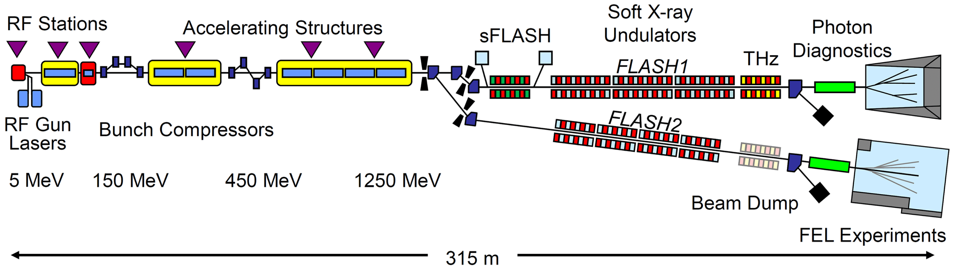
Schematic layout of FLASH (not to scale); the electron beam direction is from left to right. The total length of the facility, including the experimental halls, is 315 m.
2. SASE FELs
FLASH is a SASE FEL. The word SASE is an abbreviation for self-amplified spontaneous emission. The SASE process is a high-gain narrow-band amplification of spontaneous undulator radiation.
The SASE process was first described by Kondratenko and Saldin[Reference Kondratenko and Saldin15], theoretically explored in the early 1980s and later by many groups[Reference Derbenev, Kondratenko and Saldin16–Reference Bonifacio, De Salvo, Pierini, Piovella and Pellegrini23].
The high-gain amplification of spontaneous radiation is obtained with only one pass through a long undulator until saturation is reached. With the SASE scheme, transversely coherent laser-like radiation with femtosecond pulse durations and unprecedented brilliance in the wavelength range from the VUV, to the extreme ultraviolet (EUV), soft and hard x-ray radiation has been made possible.
There are four main challenges in the realization of x-ray FELs: first, a suitable ultra-high brightness electron source; second, a compression scheme to obtain electron bunches with high peak current of the order of 1 kA or more and at the same time small energy spread below 0.1%, together with a low emittance below  $1~{\rm\mu}\text{m}$; third, acceleration to the GeV energy scale; and fourth, precise undulator devices of several tens of meters in length, providing a high-precision undulating magnetic field (field homogeneity below 0.1%).
Today, four FEL facilities, FERMI@Elletra, Italy[24, Reference Di Mitri, Allaria, Cinquegrana, Craievich, Danailov, Demidovich, De Ninno, Diviacco, Fawley, Froehlich, Giannessi, Ivanov, Musardo, Nikolov, Penco, Sigalotti, Spampinati, Spezzani, Trovò and Veronese25], FLASH at DESY, Germany[1], LCLS at SLAC, USA[26–Reference Emma, Akre, Arthur, Bionta, Bostedt, Bozek, Brachmann, Bucksbaum, Coffee, Decker, Ding, Dowell, Edstrom, Fisher, Frisch, Gilevich, Hastings, Hays, Hering, Huang, Iverson, Loos, Messerschmidt, Miahnahri, Moeller, Nuhn, Pile, Ratner, Rzepiela, Schultz, Smith, Stefan, Tompkins, Turner, Welch, White, Wu, Yocky and Galayda28], and SACLA at SPring-8, Japan[29–Reference Ishikawa, Aoyagi, Asaka, Asano, Azumi, Bizen, Ego, Fukami, Fukui, Furukawa, Goto, Hanaki, Hara, Hasegawa, Hatsui, Higashiya, Hirono, Hosoda, Ishii, Inagaki, Inubushi, Itoga, Joti, Kago, Kameshima, Kimura, Kirihara, Kiyomichi, Kobayashi, Kondo, Kudo, Maesaka, Marchal, Masuda, Matsubara, Matsumoto, Matsushita, Matsui, Nagasono, Nariyama, Ohashi, Ohata, Ohshima, Ono, Otake, Saji, Sakurai, Sato, Sawada, Seike, Shirasawa, Sugimoto, Suzuki, Takahashi, Takebe, Takeshita, Tamasaku, Tanaka, Tanaka, Tanaka, Togashi, Togawa, Tokuhisa, Tomizawa, Tono, Wu, Yabashi, Yamaga, Yamashita, Yanagida, Zhang, Shintake, Kitamura and Kumagai32], provide femtosecond short laser-like photon pulses to user experiments. Their wavelengths range from the EUV and soft x-rays (FERMI, FLASH) to hard x-rays (LCLS, SACLA). The peak brilliance usually exceeds  $\text{10}^{\text{30}}$ photons s
 $^{-1}$ mrad
 $^{-2}$ mm
 $^{-2}$ per 0.1% bw, orders of magnitude more than third-generation synchrotron-based light sources can provide.
FERMI@Elletra’s specialty is seeding of the SASE process with an external ultraviolet laser.
Worldwide, many other soft- and hard x-ray FELs are under construction, such as the European XFEL located at DESY, Germany[33], SwissFEL at PSI, Switzerland[34, Reference Braun35], PAL-XFEL at Pohang, Korea[Reference Kang, Kim and Ko36], and LCLS-II at SLAC[Reference Galayda37].
Many articles and books have been published on free-electron lasers. An excellent introduction to ultraviolet and soft x-ray FELs is given in the book by Schmüser et al. [Reference Schmüser, Dohlus and Rossbach38] and an exhaustive discussion on the physics of FELs can be found in Saldin et al. [Reference Saldin, Schneidmiller and Yurkov39]. A brief description of FLASH and other soft and hard x-ray FELs can be found in recent reviews, for example, Refs. [Reference Schreiber40, Reference Schreiber and Brahme41], and others cited therein.
3. Description of the facility
FLASH can be divided into five basic sections: the electron source, the linac to accelerate the electron bunches, bunch compressors to provide high peak currents, the undulator systems to produce the FEL radiation, and finally several end-stations to use the radiation for research purposes.
Since 2014, FLASH has acquired a second undulator beamline, called FLASH2[Reference Faatz, Baboi, Ayvazyan, Balandin, Decking, Duesterer, Eckoldt, Feldhaus, Golubeva, Honkavaara, Koerfer, Laarmann, Leuschner, Lilje, Limberg, Noelle, Obier, Petrov, Ploenjes, Rehlich, Schlarb, Schmidt, Schmitz, Schreiber, Schulte-Schrepping, Spengler, Staack, Tavella, Tiedtke, Tischer, Treusch, Vogt, Willner, Bahrdt, Follath, Gensch, Holldack, Meseck, Mitzner, Drescher, Miltchev, Roensch-Schulenburg and Rossbach42]. After the linac, part of the beam is extracted with a kicker/septum system to the new beamline. FLASH2 has its own undulator system, beam dump and experimental stations. A detailed description of FLASH2 is given in Section 5. The layout of FLASH is sketched in Figure 1. Table 1 summarizes the main parameters of FLASH.
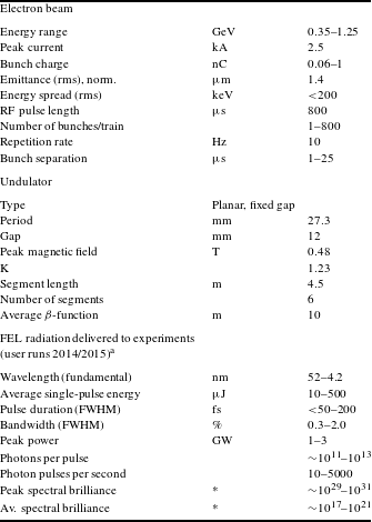
Basic FLASH electron and photon beam parameters.
* photons $/$(s mrad
 $^{2}$ mm
 $^{2}$ (0.1% bw)).
a Expected photon parameters of FLASH2 are very similar and listed in Table 2.
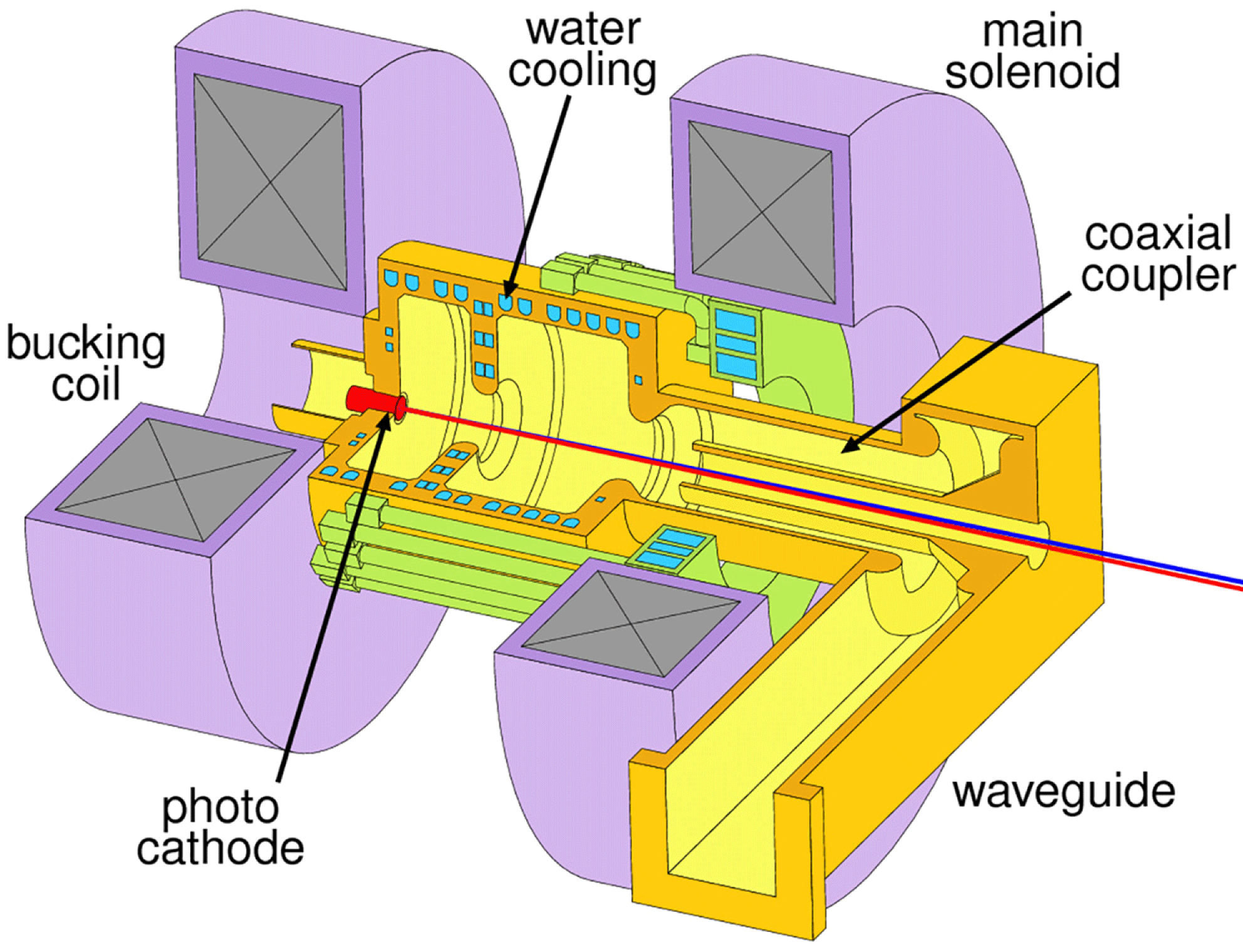
Schematic drawing of the FLASH RF-gun. The beam is emitted from the photocathode and exits to the right (path indicated by the red line). The laser beam illuminating the cathode enters along the electron beam path from the right (blue line). The RF is fed in via a coaxial waveguide coupler. Drawing courtesy: Elmar Vogel, DESY.
QE evolution of a  $\,\text{Cs}_{2}\text{Te}$ cathode in continuous operation for 436 days at FLASH.

FLASH uses 1.3 GHz TESLA superconducting accelerating technology[Reference Edwards3]. Acceleration using superconducting RF is very efficient. At FLASH, accelerating gradients exceed  $25~\text{MV}~\text{m}^{-1}$, with a usable RF pulse length of 0.8 ms at a repetition rate of 10 Hz.
These long RF pulses allow the acceleration of many electron bunches within one RF pulse, so-called bursts or pulse trains. Usually, in one RF pulse, a maximum of 800 bunches with a  $1~{\rm\mu}\text{s}$ spacing are accelerated to up to 1.25 GeV.
3.1. Electron source
As in most x-ray FEL facilities, FLASH uses a laser-driven RF-gun-based photoinjector[Reference Stephan, Boulware, Krasilnikov, Bähr, Asova, Donat, Gensch, Grabosch, Hänel, Hakobyan, Henschel, Ivanisenko, Jachmann, Khodyachykh, Khojoyan, Köhler, Korepanov, Koss, Kretzschmann, Leich, Lüdecke, Meissner, Oppelt, Petrosyan, Pohl, Riemann, Rimjaem, Sachwitz, Schöneich, Scholz, Schulze, Schultze, Schwendicke, Shapovalov, Spesyvtsev, Staykov, Tonisch, Walter, Weisse, Wenndorff, Winde, Vu, Dürr, Kamps, Richter, Sperling, Ovsyannikov, Vollmer, Knobloch, Jaeschke, Boster, Brinkmann, Choroba, Flechsenhar, Flöttmann, Gerdau, Katalev, Koprek, Lederer, Martens, Pucyk, Schreiber, Simrock, Vogel, Vogel, Rosbach, Bonev, Tsakov, Michelato, Monaco, Pagani, Sertore, Garvey, Will, Templin, Sandner, Ackermann, Arévalo, Gjonaj, Müller, Schnepp, Weiland, Wolfheimer, Rönsch and Rossbach43].
Most challenging for a free-electron laser is the requirement on the transverse projected emittance, together with a high peak current and small energy spread. As an example, a peak current 2.5 kA is achieved with a bunch length of  $50~{\rm\mu}\text{m}$ and a charge of 1 nC. Even after compression, the emittance of the lasing slice should be small, as a rough estimate below
  $1~{\rm\mu}\text{m}$. A technical solution is the RF-gun introduced by Fraser et al. in 1986[Reference Fraser, Sheffield and Gray44]. The electrons are emitted directly into a strong accelerating field from a photocathode driven with a suitable laser system. Rapid acceleration reduces space-charge-induced emittance growth, and laser-induced emission allows production of millimeter short bunches already at the cathode.
The FLASH photoinjector operates a 1 1/2-cell normal conducting 1.3 GHz L-band copper gun cavity powered by a 10 MW klystron, pulsed at 10 Hz with a RF pulse duration of up to  $900~{\rm\mu}\text{s}$. Figure 2 shows a schematic drawing of the gun.
The RF-gun is operated with a RF power of 4.5 MW fed into the standing wave gun cavity by a longitudinal RF coupler. This corresponds to a maximum field at the cathode of  $50~\text{MV}~\text{m}^{-1}$. A RF-window separates the gun vacuum from the pressured air waveguide system. Although the design allows a RF pulse length of up to
  $900~{\rm\mu}\text{s}$, we usually operate the gun at
  $500~{\rm\mu}\text{s}$ and 10 Hz to increase its lifetime. The average RF power is 25 kW. The RF-gun has no tuning paddles and no field pick-ups in the cavity. The gun is kept in tune at 1.3 GHz by controlling its temperature. The cooling water system achieves a long-term temperature stability of
  $0.015\,^{\circ }\text{C}$ (rms). The zero to pi-mode separation is 5 MHz. This is larger than the bandwidth of the klystron. A low-level RF system based on the MTCA.4 standard keeps the amplitude and phase flat over the whole pulse length[Reference Hoffmann, Butkowski, Schmidt, Schlarb, Koehler, Piotrowski, Rutkowski and Rybaniec45, Reference Schmidt, Ayvazyan, Branlard, Butkowski, Grecki, Hoffmann, Ludwig, Mavric, Pfeiffer, Przygoda, Schlarb, Weddig, Yang, Czuba, Rutkowski, Sikora, Zukocinski, Cichalewski, Makowski, Piotrowski, Kudla, Oliwa and Wierba46]. From the measured forward and reflected power using a precise directional coupler close to the gun, the vector sum is built and used for feedback. The amplitude is controlled to better than 0.01% during the flat-top RF pulse and also from shot to shot. The phase stability within the RF pulse is better than
  $0.01^{\circ }$, the shot-to-shot fluctuations are
  $0.08^{\circ }$.
A solenoid provides a focusing field of 180 mT to reduce the space-charge-induced emittance growth. The beam is then injected into the first superconducting accelerating module within a distance of 2.9 m from the cathode, optimized for smallest emittance. The solenoid field, laser spot size, and launch phase are carefully chosen to optimize beam properties. The measured projected normalized transverse rms emittance for a 1 nC bunch after acceleration to 150 MeV is smaller than the design value of  $2~{\rm\mu}\text{m}$[Reference Loehl, Schreiber, Castellano, Di Pirro, Catani, Cianchi and Honkavaara47]. With a transversely and longitudinally flat laser beam profile and increased RF power of 6 MW, the new prototype injector for FLASH and the European XFEL reaches a remarkable
  $0.7~{\rm\mu}\text{m}$ at 1 nC[Reference Krasilnikov, Stephan, Asova, Grabosch, Gross, Hakobyan, Isaev, Ivanisenko, Jachmann, Khojoyan, Klemz, Köhler, Mahgoub, Malyutin, Nozdrin, Oppelt, Otevrel, Petrosyan, Rimjaem, Shapovalov, Vashchenko, Weidinger, Wenndorff, Flöttmann, Hoffmann, Lederer, Schlarb, Schreiber, Templin, Will, Paramonov and Richter48].
The photocathode is a thin film of  $\,\text{Cs}_{2}\text{Te}$ with a diameter of 5 mm deposited on a molybdenum plug[Reference Sertore, Schreiber, Floettmann, Stephan, Zapfe and Michelato49], inserted to the RF-gun backplane via a load-lock system[Reference Sertore, Schreiber, Floettmann, Stephan, Zapfe and Michelato49]. Cathodes are prepared off site, either at INFN LASA, Milano or at DESY. They are transported in a special transport chamber with a battery back-up to maintain ultra-high vacuum conditions at all times. Figure 3 shows the quantum efficiency (QE) evolution of a cathode in continuous operation at FLASH for 436 days. The initial QE after production in May 2013 was 9.5%. FLASH produces a total charge of about 10 C per year. The laser system is designed such that a QE down to 0.5% is tolerable.
Picture of a TESLA-type 9-cell superconducting niobium cavity. The length is 1 m. Courtesy: DESY.

The dark current emitted from the RF-gun is usually below  $10~{\rm\mu}\text{A}$ for nominal operation parameters and is largely collimated by a kicker-collimation system at the gun exit, where the beam energy is still small (5.3 MeV).
FLASHhas threedrive lasers.Two of themare almost identical and are usually used to run the FLASH1 or FLASH2 beamlines. The third one has a variable pulse duration for ultra-short single-spike lasing experiments[Reference Roensch-Schulenburg, Hass, Lockmann, Plath, Rehders, Rossbach, Brenner, Dziarzhytski, Golz, Schlarb, Schmidt, Schneidmiller, Schreiber, Steffen, Stojanovic, Wunderlich and Yurkov50]. In the following, we describe the laser and beam properties in use since 2010 for the FLASH1 beamline. Details on FLASH2 will be given in Section 5. The drive laser is based on mode-locked pulse train oscillators synchronized to the 1.3 GHz RF of the accelerator. A chain of diode-pumped Nd:YLF amplifiers provides the power to convert the initial infrared wavelength into the ultraviolet (262 nm)[Reference Will, Templin, Schreiber and Sandner51] required for efficient photo emission. The ultraviolet single-pulse energy is up to  $15~{\rm\mu}\text{J}$ with a shot-to-shot stability of 0.5% (rms). The laser pulses are longitudinal Gaussian with
  ${\it\sigma}=6.25\pm 0.25~\text{ps}$. The arrival time stability measured with respect to the synchronization laser is within 80 fs (rms). The laser is able to deliver up to 800 pulses within a pulse train or burst with a minimum spacing of
  $1~{\rm\mu}\text{s}\;(1~\text{MHz})$ at 10 Hz. Several distinct spacings corresponding to frequencies between 1 MHz and 40 kHz are realized. However, due to the fixed RF pulse length of
  $800~{\rm\mu}\text{s}$, the maximum number of bunches in a train is determined by the spacing between the bunches.
At a reduced repetition rate of 5 Hz, within burst rates of 3 MHz are possible as well, thus increasing the number of pulses per burst to 2400.
The laser uses the relay-imaging technique with hard-edge spatial filtering. The laser overfills a hard-edge aperture, which is imaged onto the cathode. This yields to a transverse almost flat cut-Gaussian profile. Different aperture sizes can be used; we usually run the 1.2 mm diameter aperture for charges between 300 and 500 pC.
FLASH operates with bunch charges between a few pC and 1.2 nC, depending on the required properties of the SASE radiation. Usually, lower bunch charges are chosen for short photon pulses. The operable charge range is mainly limited by the dynamic range of diagnostics and instrumentation.
3.2. Acceleration
FLASH uses TESLA-type superconducting accelerating modules. Each module consists of eight 1 m long 9-cell standing wave solid niobium cavities with a fundamental mode frequency of 1.3 GHz (Figure 4). The cavities are bath-cooled by superfluid helium to 2 K and designed to reach an accelerating gradient of  $25~\text{MV}~\text{m}^{-1}$, some cavities even reach more than
  $30~\text{MV}~\text{m}^{-1}$. The unloaded quality factor
  $Q$ is 1 to
  $2\times \text{10}^{\text{10}}$. The loaded quality factor of the high-power RF coupler is adjusted to
  $3\times \text{10}^{\text{6}}$, the filling time is
  $500~{\rm\mu}\text{s}$ with a flat-top part for acceleration of
  $800~{\rm\mu}\text{s}$. The repetition rate is 10 Hz. For an accelerating gradient of
  $25~\text{MV}~\text{m}^{-1}$, the RF power per coupler is 250 kW. Eight cavities are mounted into one module, each equipped with one RF coupler (Figure 5). Pairs of modules (except the first one) are fed by three 5 MW Thales klystrons and one 10 MW Thales multi-beam klystron. In Figure 1 RF stations are indicated by a triangle. The klystrons are driven by a bouncer-type pulsed power supply (modulator) via a high-voltage pulse transformer.
Sketch of a TESLA-type superconducting accelerating module as installed at FLASH. The outer cryostat is not shown. Each cavity has its own RF-power coupler. Courtesy: DESY.

The length of a module is 12 m, including a quadrupole doublet, two dipole correctors, and a beam position monitor. With a total of seven modules, FLASH reaches a beam energy of 1.25 GeV, including off-crest acceleration for bunch compression. A refurbishment with new modules having high-performance cavities to increase the energy to 1.4 GeV or more is foreseen in the years to come.
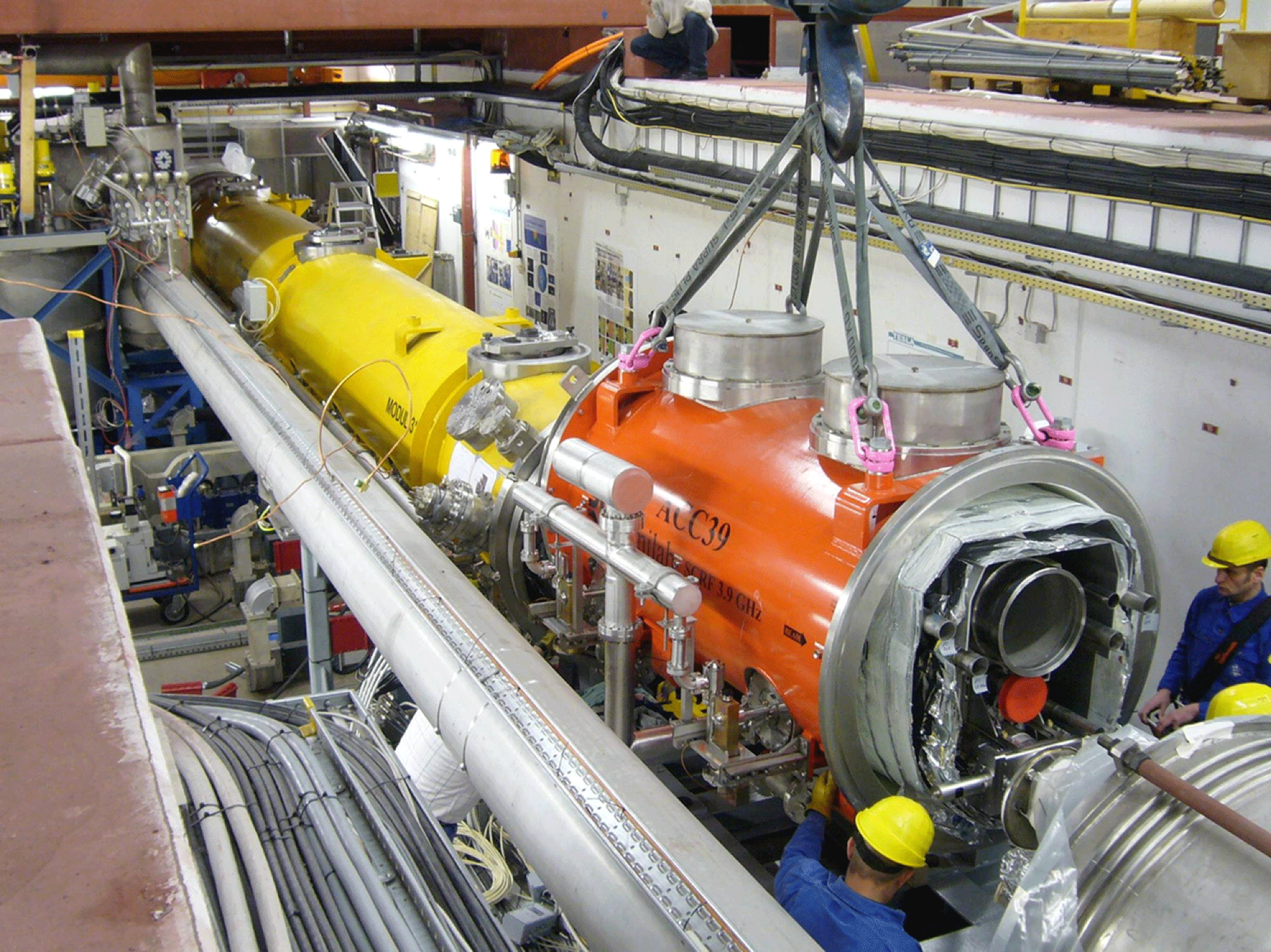
The beam from the RF-gun is immediately accelerated by one module (called ACC1) to 160 MeV. This module is fed by its own 5 MW klystron with the special feature to operate the first four cavities with reduced power. Module ACC1 is followed by a module with four third-harmonic cavities operated at 3.9 GHz. They are used to linearize the longitudinal phase space required for efficient bunch compression. A voltage of up to 21 MV can be applied, the deceleration is  $14~\text{MV}~\text{m}^{-1}$. Figure 6 shows the installation of the 3.9 GHz module into the FLASH injector in 2009. Figure 7 shows a tunnel section with accelerating modules.
Installation of the cryo-module containing four 3.9 GHz superconducting cavities (red) into the FLASH injector in 2009. The first accelerating module with eight 1.3 GHz cavities has already been installed (yellow). Courtesy: Kai Jensch, DESY.
A dedicated low-level RF system stabilizes and flattens the amplitude and phase of the accelerating fields. The vector sum of all 16 cavities connected to one RF station is calculated and stabilized. It uses sophisticated feedback and learning feedforward techniques. An excellent overview on the stabilization of the vector sum of the amplitude and phase of several cavities driven by one klystron can be found in Ref. [Reference Schilcher52].
Recently, a modern system based on the MTCA.4 technology has been brought into operation[Reference Schmidt, Ayvazyan, Branlard, Butkowski, Grecki, Hoffmann, Ludwig, Mavric, Pfeiffer, Przygoda, Schlarb, Weddig, Yang, Czuba, Rutkowski, Sikora, Zukocinski, Cichalewski, Makowski, Piotrowski, Kudla, Oliwa and Wierba46]. The new system shows a substantial improvement, by a factor of two, in performance compared to the previous system: an excellent rms amplitude stability of better than  $0.5\times \text{10}^{\text{-4}}$, and a phase stability of better than
  $0.01^{\circ }$, both over the flat-top and from pulse to pulse, is achieved.
Due to the bunch compressor chicane with an  $R_{56}$ of
  $0.18~\text{m}$, the very small remaining energy jitter translated into an excellent arrival time rms jitter of only 30 fs[Reference Schmidt, Ayvazyan, Branlard, Butkowski, Grecki, Hoffmann, Ludwig, Mavric, Pfeiffer, Przygoda, Schlarb, Weddig, Yang, Czuba, Rutkowski, Sikora, Zukocinski, Cichalewski, Makowski, Piotrowski, Kudla, Oliwa and Wierba46]. The arrival time is measured with special pick-ups correlated to an optical synchronization system[Reference Loehl, Arsov, Felber, Hacker, Jalmuzna, Lorbeer, Ludwig, Matthiesen, Schlarb, Schmidt, Schmueser, Schulz, Szewinski, Winter and Zemella53, Reference Bock, Lamb, Bousonville, Felber, Gessler, Schlarb, Schmidt, Schulz and Kuntzsch54]. Using these monitors, an arrival time feedback along the bunch trains of FLASH has been realized to the 20 fs level and better[Reference Schmidt, Bock, Pfeiffer, Schlarb, Koprek and Jalmuzna55]. Stable arrival times of less than the photon pulse duration are important for experiments using, for example, the pump–probe technique.
3.3. Bunch compression
Due to strong space-charge forces at low electron energies, it is not possible to produce bunches with a peak current exceeding 100 A directly at the source. But even for relatively small charge densities, space-charge forces may induce a growth of the projected transverse emittance. The bunch length exiting the RF-gun is  ${\it\sigma}_{z}=2~\text{mm}$ for a charge of 1 nC, long enough to reduce space-charge forces to an acceptable level. Since the space-charge forces scale with
  $1/({\it\sigma}_{z}{\it\gamma}^{2})$, compression of bunches to the kA-scale is applied at high beam energies. (
 ${\it\gamma}$ the normalized electron beam energy
  $E$:
$E$:  ${\it\gamma}=E/m_{e}c^{2}$, with
  $m_{e}$ the electron mass, and
  $c$ the speed of light.)
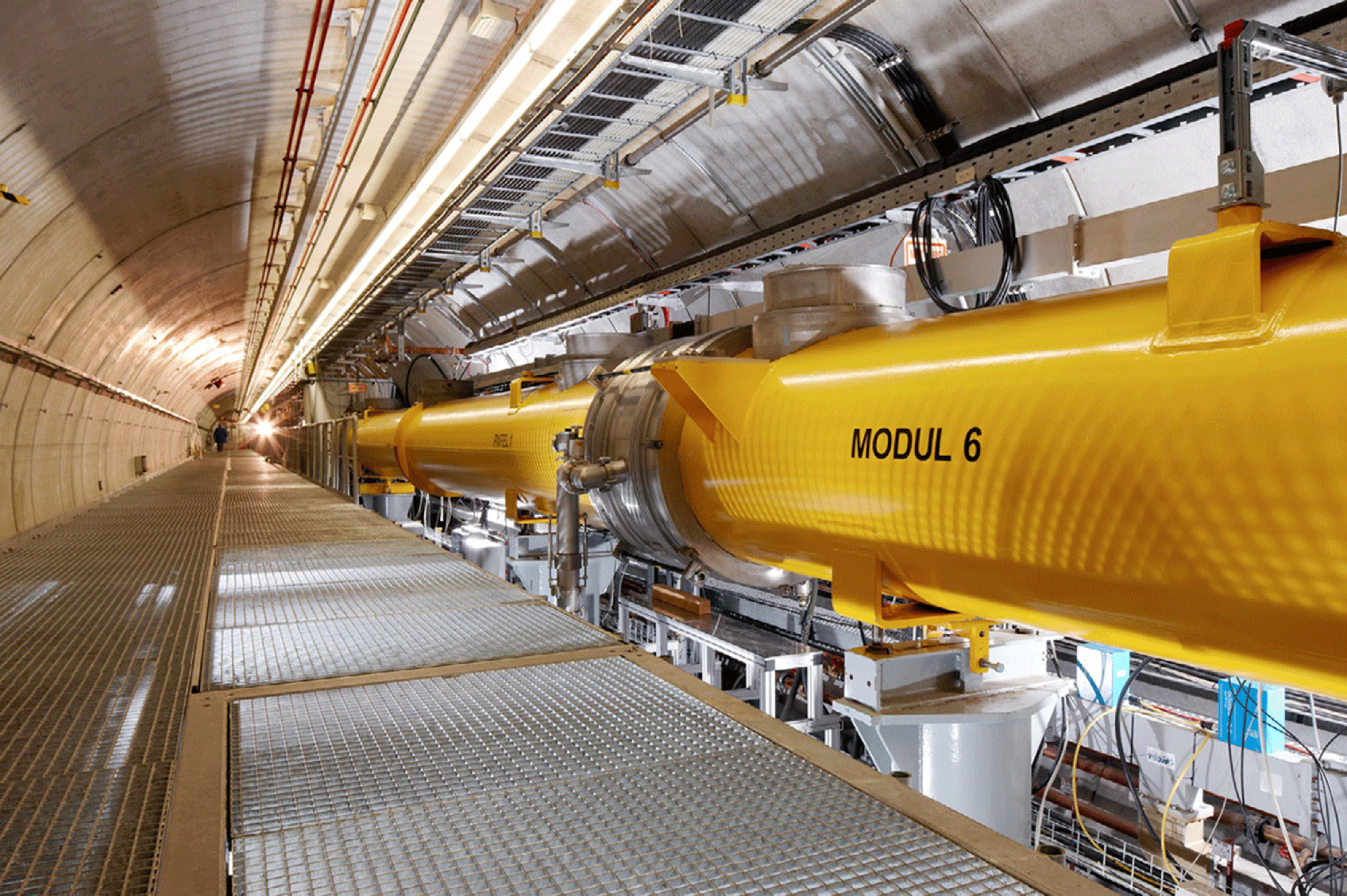
View of a FLASH tunnel section with accelerating modules. Courtesy: Heiner Müller-Elsner and DESY.
To mitigate strong space-charge effects at lower energies and large induced energy spread at higher energies, FLASH uses two magnetic chicane bunch compressors, at beam energies of 150 and 450 MeV, with  $R_{56}$ of 180 and 43 mm, respectively. Compression of relativistic electron bunches is obtained in magnetic chicanes using an energy chirp along the bunch obtained by off-crest acceleration. Due to the cosine form of the accelerating field, the chirp needs to be linearized before compression. For this, FLASH uses the four superconducting cavities installed upstream of the first compressor. They operate at 3.9 GHz, the third harmonic of 1.3 GHz. Apart from linearizing the longitudinal phase space, a proper adjustment of phase and amplitude of the cavities in the chirping modules together with the third-harmonic module allow a flexible adjustment of the compression. To a certain extent, tailoring of the bunch length and shape is possible.
For smaller charges, a stronger compression can be applied without spoiling the bunch due to space-charge effects. For example, at 1 nC, the bunch is first compressed by the first chicane to  $250~{\rm\mu}\text{m}$ and then down to
  $50~{\rm\mu}\text{m}$ (sigma) by the second chicane, achieving a peak current of 2.5 kA and a FEL pulse duration of 150 fs (FWHM). At a reduced charge of, for example, 0.2 nC, 50 fs or less can be realized.
The electron bunch duration is measured with a resolution of a few femtoseconds by frequency-domain spectroscopy of coherent transition radiation in the terahertz range[Reference Behrens, Gerasimova, Gerth, Schmidt, Schneidmiller, Serkez, Wesch and Yurkov56], and a deflecting cavity for time-domain longitudinal phase space measurements[Reference Behrens, Gerasimova, Gerth, Schmidt, Schneidmiller, Serkez, Wesch and Yurkov56].
3.4. Undulators
The FLASH1 beamline has six fixed-gap undulator segments with lengths of 4.5 m each. The undulators consist of a periodic structure of permanent NdFeB magnets with a gap of 12 mm. The peak magnetic field is 0.47 T, the undulator period 27.3 mm, and the  $K$-value 1.23 (
 $K_{\text{rms}}=0.9$). An excellent field quality has been achieved, the field is almost purely sinusoidal. The contributions from odd harmonics are very small, below 0.1% (third) and below 0.05% (fifth).
Between the six undulators, high-resolution beam-position monitors, wire scanners to measure the transverse beam profile, and a quadrupole doublet to maintain a constant beta function of about 10 m are installed.
The fundamental wavelength for radiation of a planar undulator in the forward direction is given by
 $$\begin{eqnarray}{\it\lambda}_{s}=\frac{{\it\lambda}_{u}}{2{\it\gamma}^{2}}\left(1+\frac{K^{2}}{2}\right),\end{eqnarray}$$
 where  ${\it\lambda}_{u}$ is the undulator period and
  $K$ is the dimensionless undulator parameter. For a planar undulator,
  $K$ is defined as
 $$\begin{eqnarray}K=\frac{eB_{o}{\it\lambda}_{u}}{2{\it\pi}m_{e}c},\end{eqnarray}$$
 where  $e$ is the electron charge and
  $B_{o}$ the peak magnetic field on the undulator axis.
An important consequence of Equation (1) is the apparently unlimited tunability of the radiation by choosing the right electron beam energy. Wavelength tuning is also possible by changing the undulator parameter  $K$. This is realized in variable gap undulators:
  $K$ changes with the gap height due to the change of
  $B_{o}$.
In practice, with beam energies between 350 MeV and 1.25 GeV, lasing at wavelengths between 52 and 4.1 nm is achieved with the FLASH1 fixed-gap undulators. The third, and sometimes the fifth, harmonics of the fundamental wavelength are also used for experiments.
3.5. Photon diagnostics
The undulator is followed by a photon diagnostics section and a photon beamline to transport the FEL radiation to the experimental hall, where the user experiments are located. A comprehensive overview of the FLASH photon diagnostics is given in Ref. [Reference Tiedtke, Azima, von Bargen, Bittner, Bonfigt, Duesterer, Faatz, Fruehling, Gensch, Gerth, Guerassimova, Hahn, Hans, Hesse, Honkavaara, Jastrow, Juranic, Kapitzki, Keitel, Kracht, Kuhlmann, Li, Martins, Nunez, Ploenjes, Redlin, Saldin, Schneidmiller, Schneider, Schreiber, Stojanovic, Tavella, Toleikis, Treusch, Weigelt, Wellhoefer, Wabnitz, Yurkov and Feldhaus57].
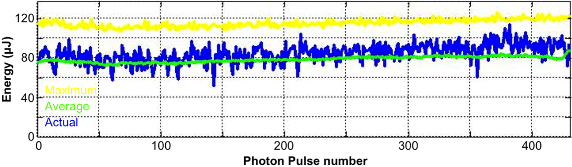
The transverse size and position of the photon beam are measured with Ce:YAG screen monitors. The energies of the FEL radiation pulses are measured with absolutely calibrated gas-monitor detectors (GMDs)[Reference Richter, Gottwald, Kroth, Sorokin, Bobashev, Shmaenok, Feldhaus, Gerth, Steeg, Tiedtke and Treusch58, Reference Tiedtke, Feldhaus, Hahn, Jastrow, Nunez, Tschentscher, Bobashev, Sorokin, Hastings, Moeller, Cibik, Gottwald, Hoehl, Kroth, Krumrey, Schoeppe, Ulm and Richter59]. They are based on photoionization of gases with well known cross-sections. The detectors have a large dynamic range covering the full spectral range and several orders of magnitude in energy from spontaneous emission to saturation. The electron signal of the GMD resolves single pulses within a pulse train. Figure 8 shows a train of 430 FEL pulses measured with a GMD. The GMDs are also used to measure the transverse position of the photon beam.
The FEL radiation spectrum is measured by high-resolution spectrometers. Online, non-destructive spectrometers are also available.
Photon energy along a photon pulse train of 430 pulses measured with a GMD at FLASH. The detector is able to resolve single FEL pulses (blue line). Also shown are the average over many shots (green) and maximum energies recorded (yellow). In this example, the wavelength is 18.2 nm, the pulse spacing  $1~{\rm\mu}\text{s}$. With a single-pulse energy of
  $80~{\rm\mu}\text{J}$ and 4300 pulses per second, the average SASE power is 350 mW.
3.6. Transverse coherence
SASE radiation is expected to have a high degree of transverse coherence. Measurements at FLASH at a wavelength of 13.7 nm with a double-slit system show an almost full transverse coherence[Reference Singer, Vartanyants, Kuhlmann, Duesterer, Treusch and Feldhaus60]. The double-slit measurement demonstrates that the degree of coherence is similar for the horizontal and vertical direction, and that the coherence length is about  $300\pm 15~{\rm\mu}\text{m}$ at a distance of 20 m downstream of the undulator. In another experiment, a transverse coherence length of 2.3 mm (rms) has been measured at a wavelength of 24 nm, this time at the experimental station (spot size 2.5 mm rms) and with a 3 mm aperture 20 m downstream of the undulator[Reference Roling, Siemer, Woestmann, Zacharias, Mitzner, Singer, Tiedtke and Vartanyants61].
It is important to mention that, in deep saturation, higher modes gain in energy with respect to the fundamental mode, with the consequence of a reduced transverse coherence. For a more detailed discussion on coherence properties the reader is referred to Saldin et al. [Reference Saldin, Schneidmiller and Yurkov62], and on experiments at FLASH to Roling et al. [Reference Roling, Siemer, Woestmann, Zacharias, Mitzner, Singer, Tiedtke and Vartanyants61]. A recent discussion on coherence properties of radiation at FLASH points out that the temporal and spatial coherence reach a maximum close to saturation, but may degrade significantly in the post-saturation regime, and that the pointing stability of the radiation may be limited by non-azimuthal eigenmodes[Reference Schneidmiller and Yurkov63].
3.7. Coherence time and pulse duration
Other important properties of SASE radiation are the spectral content, the coherence time and pulse duration.
The stochastic nature of the SASE process is responsible for the intrinsic fluctuation of the energy and wavelength spectra of the amplified FEL radiation.
Figure 9 shows examples of single-shot spectra measured at FLASH. The single-shot spectra vary in center wavelength and shape. The bold curve in Figure 9 is an averaged spectrum over 300 shots. In this example, the single-shot spectra sometimes show a single spike – but often two, three or more spikes are visible. This is also true in time domain: also the temporal profile of the radiation pulses consists of a couple of spikes, varying from shot to shot.
Measured single-shot spectra at FLASH. The bold line shows an averaged spectrum over 300 shots. The spectra are obtained in saturation. The circles indicate a simulation of the averaged spectrum with the 3D code FAST[Reference Saldin, Schneidmiller and Yurkov64]. Adapted from Ref. [Reference Ackermann, Asova, Ayvazyan, Azima, Baboi, Bhr, Balandin, Beutner, Brandt, Bolzmann, Brinkmann, Brovko, Castellano, Castro, Catani, Chiadroni, Choroba, Cianchi, Costello, Cubaynes, Dardis, Decking, Delsim-Hashemi, Delserieys, Di Pirro, Dohlus, Düsterer, Eckhardt, Edwards, Faatz, Feldhaus, Flöttmann, Frisch, Fröhlich, Garvey, Gensch, Gerth, Görler, Golubeva, Grabosch, Grecki, Grimm, Hacker, Hahn, Han, Honkavaara, Hott, Hüning, Ivanisenko, Jaeschke, Jalmuzna, Jezynski, Kammering, Katalev, Kavanagh, Kennedy, Khodyachykh, Klose, Kocharyan, Körfer, Kollewe, Koprek, Korepanov, Kostin, Krassilnikov, Kube, Kuhlmann, Lewis, Lilje, Limberg, Lipka, Löhl, Luna, Luong, Martins, Meyer, Michelato, Miltchev, Möller, Monaco, Müller, Napieralski, Napoly, Nicolosi, Nölle, Nuez, Oppelt, Pagani, Paparella, Pchalek, Pedregosa-Gutierrez, Petersen, Petrosyan, Petrosyan, Petrosyan, Pflüger, Plönjes, Poletto, Pozniak, Prat, Proch, Pucyk, Radcliffe, Redlin, Rehlich, Richter, Roehrs, Roensch, Romaniuk, Ross, Rossbach, Rybnikov, Sachwitz, Saldin, Sandner, Schlarb, Schmidt, Schmitz, Schmüser, Schneider, Schneidmiller, Schnepp, Schreiber, Seidel, Sertore, Shabunov, Simon, Simrock, Sombrowski, Sorokin, Spanknebel, Spesyvtsev, Staykov, Steffen, Stephan, Stulle, Thom, Tiedtke, Tischer, Toleikis, Treusch, Trines, Tsakov, Vogel, Weiland, Weise, Wellhöfer, Wendt, Will, Winter, Wittenburg, Wurth, Yeates, Yurkov, Zagorodnov and Zapfe8]. Adapted by permission from Macmillan: Nature Photonics, [Reference Ackermann, Asova, Ayvazyan, Azima, Baboi, Bhr, Balandin, Beutner, Brandt, Bolzmann, Brinkmann, Brovko, Castellano, Castro, Catani, Chiadroni, Choroba, Cianchi, Costello, Cubaynes, Dardis, Decking, Delsim-Hashemi, Delserieys, Di Pirro, Dohlus, Düsterer, Eckhardt, Edwards, Faatz, Feldhaus, Flöttmann, Frisch, Fröhlich, Garvey, Gensch, Gerth, Görler, Golubeva, Grabosch, Grecki, Grimm, Hacker, Hahn, Han, Honkavaara, Hott, Hüning, Ivanisenko, Jaeschke, Jalmuzna, Jezynski, Kammering, Katalev, Kavanagh, Kennedy, Khodyachykh, Klose, Kocharyan, Körfer, Kollewe, Koprek, Korepanov, Kostin, Krassilnikov, Kube, Kuhlmann, Lewis, Lilje, Limberg, Lipka, Löhl, Luna, Luong, Martins, Meyer, Michelato, Miltchev, Möller, Monaco, Müller, Napieralski, Napoly, Nicolosi, Nölle, Nuez, Oppelt, Pagani, Paparella, Pchalek, Pedregosa-Gutierrez, Petersen, Petrosyan, Petrosyan, Petrosyan, Pflüger, Plönjes, Poletto, Pozniak, Prat, Proch, Pucyk, Radcliffe, Redlin, Rehlich, Richter, Roehrs, Roensch, Romaniuk, Ross, Rossbach, Rybnikov, Sachwitz, Saldin, Sandner, Schlarb, Schmidt, Schmitz, Schmüser, Schneider, Schneidmiller, Schnepp, Schreiber, Seidel, Sertore, Shabunov, Simon, Simrock, Sombrowski, Sorokin, Spanknebel, Spesyvtsev, Staykov, Steffen, Stephan, Stulle, Thom, Tiedtke, Tischer, Toleikis, Treusch, Trines, Tsakov, Vogel, Weiland, Weise, Wellhöfer, Wendt, Will, Winter, Wittenburg, Wurth, Yeates, Yurkov, Zagorodnov and Zapfe8], Copyright (2007).

Within one coherence time all electrons radiate in phase, resulting in a temporally coherent ‘spike’. Due to the slippage effect (the radiated photons travel faster than the electrons), many spikes build up along the electron bunch, with a random phase relationship between them[Reference Bonifacio, De Salvo, Pierini, Piovella and Pellegrini23].
At FLASH, a first estimate of the coherence time at a wavelength of 13.7 nm was deduced from experimental data to be a few femtoseconds: 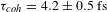 ${\it\tau}_{coh}=4.2\pm 0.5~\text{fs}$[Reference Ackermann, Asova, Ayvazyan, Azima, Baboi, Bhr, Balandin, Beutner, Brandt, Bolzmann, Brinkmann, Brovko, Castellano, Castro, Catani, Chiadroni, Choroba, Cianchi, Costello, Cubaynes, Dardis, Decking, Delsim-Hashemi, Delserieys, Di Pirro, Dohlus, Düsterer, Eckhardt, Edwards, Faatz, Feldhaus, Flöttmann, Frisch, Fröhlich, Garvey, Gensch, Gerth, Görler, Golubeva, Grabosch, Grecki, Grimm, Hacker, Hahn, Han, Honkavaara, Hott, Hüning, Ivanisenko, Jaeschke, Jalmuzna, Jezynski, Kammering, Katalev, Kavanagh, Kennedy, Khodyachykh, Klose, Kocharyan, Körfer, Kollewe, Koprek, Korepanov, Kostin, Krassilnikov, Kube, Kuhlmann, Lewis, Lilje, Limberg, Lipka, Löhl, Luna, Luong, Martins, Meyer, Michelato, Miltchev, Möller, Monaco, Müller, Napieralski, Napoly, Nicolosi, Nölle, Nuez, Oppelt, Pagani, Paparella, Pchalek, Pedregosa-Gutierrez, Petersen, Petrosyan, Petrosyan, Petrosyan, Pflüger, Plönjes, Poletto, Pozniak, Prat, Proch, Pucyk, Radcliffe, Redlin, Rehlich, Richter, Roehrs, Roensch, Romaniuk, Ross, Rossbach, Rybnikov, Sachwitz, Saldin, Sandner, Schlarb, Schmidt, Schmitz, Schmüser, Schneider, Schneidmiller, Schnepp, Schreiber, Seidel, Sertore, Shabunov, Simon, Simrock, Sombrowski, Sorokin, Spanknebel, Spesyvtsev, Staykov, Steffen, Stephan, Stulle, Thom, Tiedtke, Tischer, Toleikis, Treusch, Trines, Tsakov, Vogel, Weiland, Weise, Wellhöfer, Wendt, Will, Winter, Wittenburg, Wurth, Yeates, Yurkov, Zagorodnov and Zapfe8].
Several direct measurements of the coherence time have been carried out at FLASH with a split-and-delay autocorrelation experiment[Reference Roling, Siemer, Woestmann, Zacharias, Mitzner, Singer, Tiedtke and Vartanyants61, Reference Siemer, Neeb, Noll, Siewert, Roling, Rutkowski, Sorokin, Richter, Juranic, Tiedtke, Feldhaus, Eberhardt and Zacharias65, Reference Schlotter, Sorgenfrei, Beeck, Beye, Gieschen, Meyer, Nagasono, Föhlisch and Wurth66]. A recent study measured the coherence time as a function of wavelength  ${\it\lambda}$, demonstrating the nonlinear dependence
  ${\it\tau}_{coh}\propto \sqrt{{\it\lambda}}$ [Reference Roling, Siemer, Woestmann, Zacharias, Mitzner, Singer, Tiedtke and Vartanyants61]. For example, at 24 and 8 nm
  ${\it\tau}_{coh}=6\pm 0.5~\text{fs}$ and
 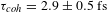 ${\it\tau}_{coh}=2.9\pm 0.5~\text{fs}$, respectively, have been measured.
Time-resolved double ionization of He (dots). The solid line is a Gaussian fit to the autocorrelation data with a width of 39 fs (FWHM). Assuming a Gaussian FEL pulse shape, this gives a duration of  ${\it\tau}_{s}=29\pm 5~\text{fs}$ (FWHM). The dashed line represents a three-pulse structure with temporal separations of the side peaks by 12 and 40 fs, with an added chirp of 50 fs
 $^{2}$. Reprinted with permission from Ref. [Reference Mitzner, Sorokin, Siemer, Roling, Rutkowski, Zacharias, Neeb, Noll, Siewert, Eberhardt, Richter, Juranic, Tiedtke and Feldhaus67]. Copyright (2009) by the American Physical Society.

There have also been several experiments to measure the photon pulse duration. As an example, the split-and-delay autocorrelator was used together with two-photon double ionization of He as a nonlinear medium. Figure 10 shows the time-resolved yield of double ionized He[Reference Mitzner, Sorokin, Siemer, Roling, Rutkowski, Zacharias, Neeb, Noll, Siewert, Eberhardt, Richter, Juranic, Tiedtke and Feldhaus67]. From a fit to the data, a pulse duration of  ${\it\tau}_{s}=29\pm 5~\text{fs}$ (FWHM) has been derived. The plot also shows as a dashed line the spike structure of the FEL pulse in time domain.
Another measurement of the pulse duration at FLASH at a wavelength of 13.5 nm gives a pulse duration of  ${\it\tau}_{s}=37\pm 7~\text{fs}$ (FWHM)[Reference Fruehling, Wieland, Gensch, Gebert, Schuette, Krikunova, Kalms, Budzyn, Grimm, Rossbach, Ploenjes and Drescher68]. This time a streak technique with THz radiation from the FLASH THz undulator was used.
Recently, a series of experiments have been carried out at FLASH to measure the photon pulse duration and the electron bunch length at the same time via nine different methods[Reference Düsterer, Rehders, Al-Shemmary, Behrens, Brenner, Brovko, DellAngela, Drescher, Faatz, Feldhaus, Frühling, Gerasimova, Gerken, Gerth, Golz, Grebentsov, Hass, Honkavaara, Kocharian, Kurka, Limberg, Mitzner, Moshammer, Plönjes, Richter, Rönsch-Schulenburg, Rudenko, Schlarb, Schmidt, Senftleben, Schneidmiller, Siemer, Sorgenfrei, Sorokin, Stojanovic, Tiedtke, Treusch, Vogt, Wieland, Wurth, Wesch, Yan, Yurkov, Zacharias and Schreiber69]. One result is that the duration of the photon pulse is usually shorter by a factor of roughly two than the electron bunch generating the SASE radiation.
4. FLASH operation
FLASH is a user facility. The first call for user experiments has been launched in 2005. The facility hosts many experiments, ranging from atomic physics through materials science to biology.
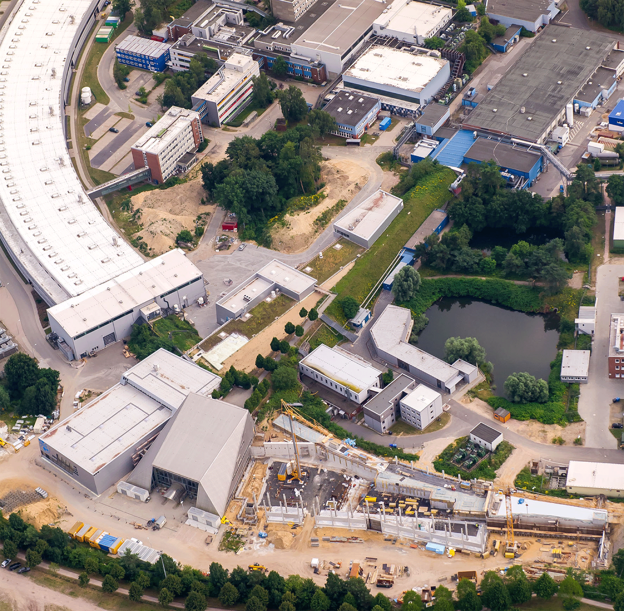
Aerial view of the FLASH Facility at DESY, Hamburg. The accelerator is from top right to the lower left, with the two experimental halls; Kai Siegbahn hall (left) and Albert Einstein hall (right) in the lower left corner. The curved hall (left) and the construction site (bottom) belong to the synchrotron radiation facility PETRA III. Courtesy: DESY, July 2014.
FLASH provides 4500 h beamtime per year for external user experiments. User experiments are overbooked by a factor of three to four. The beam can only be served for one experiment at a given time. In addition, 2250 h of beamtime is used to prepare user experiments, and for photon beamline and accelerator related studies to improve the performance of the facility. Part of the beamtime is dedicated to general accelerator-related research and development (750 h). This includes testing beam instrumentation and other equipment for the European XFEL. FLASH has also been a test bed for the International Linear Collider Project.
User experiments are schedules in blocks of four weeks. The two or three weeks time between the blocks is used to swap the experiments and to prepare the beamlines for the next experiments. Part of the time is also used for the studies described above.
In a typical week, two or three experiments are served with beam alternating from day to day. As a consequence, the wavelength at FLASH is often changed on a day to day basis. As described in Section 3.4, the wavelength at FLASH1 is changed by changing the beam energy. This is especially difficult for low beam energies where space-charge forces are more dominant. Depending on the required bunch length, space-charge-induced effects vary with beam energy in a nonlinear way, which makes a wavelength change non-trivial and time consuming. Together with other requests, such as pulse duration, spectral width, many pulses per second all with the same properties, correct and stable pointing, etc., this results in a substantial tuning time of about 20% of the time allocated for user experiments.
With the construction of the second beamline FLASH2, we will be able to double the available beamtime, and to ease wavelength tuning by providing variable gap undulators.
5. The new undulator beamline FLASH2
FLASH2, the second undulator beamline, was constructed between late 2011 and early 2014[Reference Honkavaara, Faatz, Feldhaus, Schreiber, Treusch and Vogt12, Reference Faatz, Baboi, Ayvazyan, Balandin, Decking, Duesterer, Eckoldt, Feldhaus, Golubeva, Honkavaara, Koerfer, Laarmann, Leuschner, Lilje, Limberg, Noelle, Obier, Petrov, Ploenjes, Rehlich, Schlarb, Schmidt, Schmitz, Schreiber, Schulte-Schrepping, Spengler, Staack, Tavella, Tiedtke, Tischer, Treusch, Vogt, Willner, Bahrdt, Follath, Gensch, Holldack, Meseck, Mitzner, Drescher, Miltchev, Roensch-Schulenburg and Rossbach42, Reference Ayvazyan, Baboi, Balandin, Decking, Duesterer, Eckoldt, Faatz, Felber, Feldhaus, Golubeva, Honkavaara, Koerfer, Laarmann, Leuschner, Lilje, Limberg, Noelle, Obier, Petrov, Ploenjes, Rehlich, Schlarb, Schmidt, Schmitz, Schreiber, Schulte-Schrepping, Spengler, Staack, Tiedtke, Tischer, Treusch, Vogt, Weddig, Bahrdt, Follath, Holldack, Meseck, Mitzner, Drescher, Hage, Miltchev, Riedel, Roensch-Schulenburg, Rossbach, Schulz, Willner, Tavella, Gensch, Liu, Chen and Deng70]. Figure 11 shows an aerial view of the facility. A new building for the FLASH2 undulator beamline has been built along the old FLASH1 tunnel. The building is large enough to house a third beamline in the future. For the connection to the FLASH accelerator, an opening has been cut into the old FLASH1 tunnel.
The main features of FLASH2 are to double the available beamtime for experiments, to provide more flexibility with variable gap undulators, and – at a later stage – to include seeding options. A second experimental hall completes the beamline, with space for up to seven experimental stations.
The new beamline makes full use of the existing accelerator of FLASH. Part of the bunch train is extracted after acceleration from the main accelerator at a shallow angle of  $12^{\circ }$[Reference Scholz, Faatz, Vogt and Zemella71] to the right in the direction of the new beamline (see also the FLASH layout in Figure 1).
Figure 12 shows the basic scheme: the electrons are accelerated in bursts or trains, as described in Section 3. This train is now separated into two parts, one to be sent to the FLASH1 beamline, the other to FLASH2. A kicker–septum system provides a fast separation within  $30~{\rm\mu}\text{s}$. The gap between the sub-trains is large enough to ramp up the kicker system.
Both beamlines are thus operated with the repetition rate of the accelerator, essentially doubling the available beamtime.
Basic scheme for splitting the bunch trains. The train is split into two parts, one to be sent to the FLASH1 beamline, the other to FLASH2. The gap between the sub-trains is large enough to ramp up the kicker system.

5.1. Simultaneous operation of FLASH1 and FLASH2
Even though FLASH is able to deliver several hundred photon pulses in one pulse train to experiments with a repetition rate of 10 Hz, not all users fully use this feature. In practice, about half of the users request long pulse trains for their experiments, whereas the others ask for a single pulse or a few pulses only. Therefore, it is hardly a limitation to deliver a beam to two users simultaneously with one user receiving only single bunch or a few bunches, provided that all other parameters can be chosen as flexibly as possible. Table 2 shows the expected parameters for the FLASH2 beamline.
Expected parameters for FLASH2.

* photons/(s mrad $^{2}$ mm
 $^{2}$ (0.1% bw)).
a This includes a headroom of  $50~{\rm\mu}\text{s}$ for a FLASH1 beam with a few bunches only.
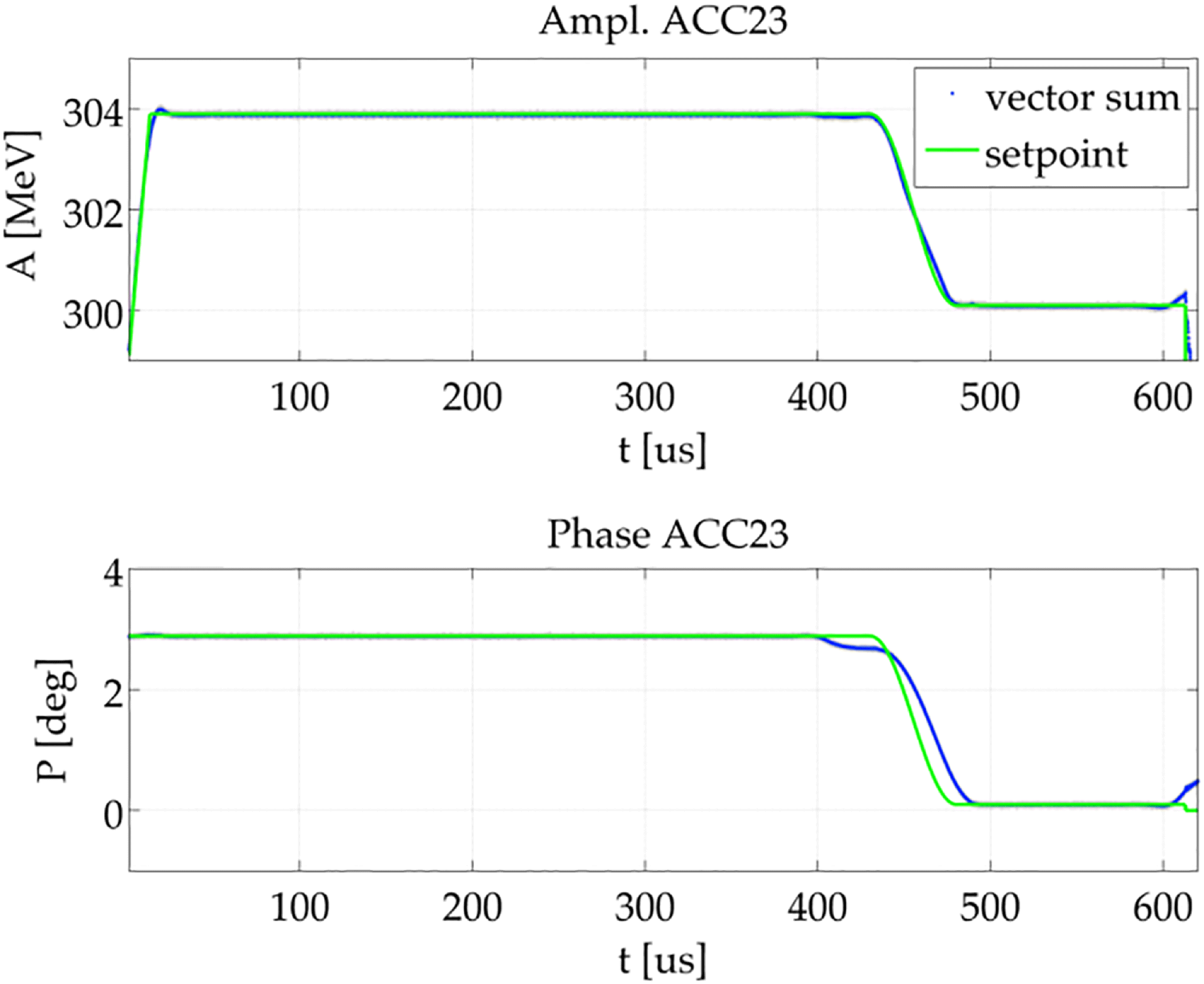
An example of the steps in amplitude (top) and phase (bottom) within a RF pulse in one of the modules, needed to optimize compression for different charges at FLASH1 and FLASH2. The part from 0 to  $400~{\rm\mu}\text{s}$ is for the sub-train to be sent to FLASH1, the part from 500 to
  $600~{\rm\mu}\text{s}$ is for FLASH2. The position where the step occurs is adjustable according to the length of each sub-train. The green curves show the setpoint for the step and the blue curves show the achieved step.
The obvious parameter which needs to be independent for both experiments is the wavelength. Therefore, the FLASH2 undulator has a variable gap, with which the wavelength can be tuned by roughly a factor of four for each beam energy. The correct undulator gap is set by measuring the electron beam energy and automatically setting the gap for the desired wavelength.
A second important parameter needed by the users is the pulse duration of the photon pulse. In order to achieve this, the charge needs to be different for both undulators and the compression must be different as well. A different charge is achieved by using two different injector lasers. This also ensures that different numbers of bunches and different bunch separations can be set easily as well. Because these bunch trains have different space charges, to realize different bunch lengths, each sub-train requires a different compression scheme. This is done by adjusting the RF amplitude and phase of each RF station separately for each sub-train. Figure 13 shows an example of the split RF scheme.
Tests have shown that changes in all RF stations are needed, even though one might expect that only changes are needed at lower energy and those stations where the beam is compressed. In fact, in practice we have seen that also a slight deviation in energy is necessary to obtain optimal performance for both beamlines.
Example of simultaneous SASE at FLASH1 with single-bunch operation (left) and FLASH2 with 10 bunches (right) measured with GMDs. The top plots show the calibrated ion signal, the bottom row the single-shot electron signals resolving each pulse in the pulse train. The blue color indicates the last value. In addition, average (green) and peak values (yellow) are displayed as well. Note that the FLASH2 GMD is not yet calibrated.

Examples for lasing at FLASH1 and FLASH2 are shown in Figure 14. Since the detector at FLASH2 is not calibrated yet, only arbitrary units are shown for this beamline. In the case shown, the electron beam energy was around 0.7 GeV, which corresponds to a wavelength of around 13 nm for the FLASH1 fixed-gap undulator. While the FLASH1 FEL beam was used by users for an ongoing experiment, the wavelength of the photon beam at FLASH2 was varied by changing the undulator gap, resulting in wavelengths between 40 and 11 nm. The 12 nm point is shown in Figure 14. Similar tests of the wavelength tuning range have been performed at electron beam energies between 0.55 and 1.2 GeV. The bunch number at FLASH1 has been between 1 and 400, with a 10 Hz repetition rate, whereas in FLASH2, the bunch number so far has been limited to a maximum of 11 bunches. Full beam in FLASH2 will be possible when the radiation shielding is finalized in spring 2015.
Acknowledgements
We would like to thank the FLASH team, the FLASH operators, the DESY support groups, and collaborating institutes for their tremendous efforts to make FLASH a worldwide leading FEL user facility. We especially thank the FLASH II project team and supporting groups for their excellent work in building and commissioning the fantastic new FLASH2 beamline.


 Open access