2. Approach

For compressible homogeneous flows, Ristorcelli (Reference Ristorcelli1997) expressed quantities such as pressure, density and velocity in the form of expansion series as follows:

(2.1) \begin{equation} \begin{aligned} p^{\prime } / \mathcal{P} &= \epsilon ^2 \big [ p_1^{\prime } / \big(\rho _\infty \mathcal{U}^2 \big) + \epsilon ^2\, p_2^{\prime } / \big(\rho _\infty \mathcal{U}^2 \big) + {\epsilon ^4\, p_3^{\prime } / \big(\rho _\infty \mathcal{U}^2 \big)} + \cdots \big ], \\\rho ^{\prime } / \rho _\infty &= \epsilon ^2 \big [ \rho _1^{\prime } / \rho _\infty + \epsilon ^2\, \rho _2^{\prime } / \rho _\infty {+ \epsilon ^4\, \rho _3^{\prime } / \rho _\infty } + \cdots \big ], \\u_i / \mathcal{U} &= u_{0i} / \mathcal{U} + \epsilon ^2 \big [ u_{1i} / \mathcal{U} + \epsilon ^2\, u_{2i} / \mathcal{U} + {\epsilon ^4\, u_{3i} / \mathcal{U}} + \cdots \big ], \end{aligned} \end{equation}

where $\mathcal P$ is the thermodynamic scale of pressure, $\mathcal U$ is the velocity scale, $\rho _\infty$ is the reference background density, ${\epsilon ^2} = \rho _\infty \mathcal U^2/\mathcal P$ is the ratio of the hydrodynamic scale of pressure $\rho _\infty \mathcal U^2$ to the thermodynamic scale, and the subscripts 0, 1, 2, 3 signify the order of the variables. Here, the single prime denotes fluctuations from Reynolds average. When these expansions are substituted into the Navier–Stokes equations, and the terms with similar powers of $\epsilon$ are grouped, it produces a set of zeroth-order (proportional to $\epsilon ^0$ ), first-order (proportional to $\epsilon ^2$ ) and higher-order governing equations. The zeroth-order set of equations solves for the incompressible velocity $u_{0i}$ and pressure $p_1^\prime$ , whereas the higher-order equations solve for the higher order variables. (Note that since the pressure term in the Navier–Stokes equation, upon appropriate non-dimensionalisation, is multiplied with $\epsilon ^{-2}$ , a first-order pressure $p_1^\prime$ acts as the incompressible pressure to satisfy a meaningful balance between velocity and pressure terms; Ristorcelli Reference Ristorcelli1997.)

It is worth noting that in these expansions, Ristorcelli (Reference Ristorcelli1997) assumed the thermodynamic scale of pressure to be the reference background pressure $P_\infty$ , and the velocity scale to be $(2 k/3)^{1/2}$ , where $k$ is the turbulent kinetic energy defined as $k = \overline {u_i^{\prime }u_i^{\prime }}/2$ , with the overline denoting Reynolds averaging. This gives $\epsilon ^2 = \rho _\infty (2k/3)/P_\infty$ , which is equal to $\gamma M_t^2$ for ideal gas flows, where $\gamma$ is the ratio of specific heats, and $M_t =(2 k/3)^{1/2}/c_\infty$ , with $c_\infty$ being the reference speed of sound.

Let us now extend Ristorcelli’s approach to compressible wall-bounded flows, but with some notable differences. For homogeneous flows, Ristorcelli (Reference Ristorcelli1997) represented the compressible flow field as a sum of an incompressible field and higher-order fields, with the latter capturing effects that arise only at finite Mach numbers. In the same spirit, we represent a compressible wall-bounded flow field as a sum of a variable-property zero-Mach-number field – i.e. the flow field that would exist in a variable-property flow at zero Mach number with the same Reynolds number and mean property distributions as the compressible flow – and higher-order fields representative of finite-Mach-number effects. Such an expansion ensures that the zeroth-order term in the expansion series comprises variable-property and Reynolds number effects, such that the higher-order terms primarily represent intrinsic compressibility effects that occur only at finite Mach numbers.

Some other differences are as follows. Since the base (zeroth-order) state about which the expansion series is built represents a zero-Mach-number flow with mean property variations, the reference density $\rho _\infty$ and $c_\infty$ in Ristorcelli’s work should be replaced with the local mean density $\bar \rho$ and the local mean speed of sound $\bar c$ , respectively. Additionally, the semi-local friction velocity scale $u_\tau ^*$ becomes the relevant scale in compressible wall-bounded flows, instead of $(2k/3)^{1/2}$ . Finally, we choose the thermodynamic pressure scale to be $\bar \rho \bar c^2$ rather than $\bar p$ , for the following reason. The isentropic density fluctuations are related to pressure fluctuations through the relation $ {({\rho ^\prime })^{\textit{is}}}/{\bar \rho } \approx {p^{\prime }}/({\bar \rho \bar c^2})$ (Hasan et al. Reference Hasan, Costa, Larsson, Pirozzoli and Pecnik2025). This implies that the density fluctuations depend on $\bar \rho \bar c^2$ . Since intrinsic compressibility effects are, by definition, related to isentropic density fluctuations, it is natural that the parameter characterising these effects – namely, $\epsilon$ – also depends on $\bar \rho \bar c^2$ . Taking $\mathcal{P}= \bar \rho \bar c^2$ , along with $\bar \rho {u_\tau ^*}^2$ as the hydrodynamic pressure scale, we get

(2.2) \begin{equation} \epsilon ^2 = {\bar \rho {u_\tau ^*}^2}/ \big({\bar \rho \bar c^2} \big) = {M_\tau ^*}^2. \end{equation}

By accounting for these differences, we get the expansion series for pressure fluctuations in wall-bounded flows (analogous to (2.1) for homogeneous flows) as

(2.3) \begin{equation} p^{\prime } / \big(\bar {\rho } \bar {c}^2 \big) = {M_\tau ^*}^2 \big [ p_1^{\prime } / \big(\bar {\rho } {u_\tau ^*}^2 \big) + {M_\tau ^*}^2\, p_2^{\prime } / \big(\bar {\rho } {u_\tau ^*}^2 \big) +{ {M_\tau ^*}^4\, p_3^{\prime } / \big(\bar {\rho } {u_\tau ^*}^2 \big)} + \cdots \big ]. \end{equation}

By writing this equation at the wall, squaring it, averaging, and dividing by ${M_\tau ^*}^4$ , we get the equation for wall-pressure variance, scaled by $\tau _w^2$ , as

(2.4) \begin{equation} {\overline {p^{\prime }p^{\prime }}}_w^+ = \overline {p^{\prime }_1p^{\prime }_1}_w^+ + {M_\tau ^*}^2 \big [ 2\, \overline { p^{\prime }_1p^{\prime }_2}_w^+ + {M_\tau ^*}^2 \big(\overline {p^{\prime }_2 p^{\prime }_2}_w^+ + 2 \overline { p^{\prime }_1 p^{\prime }_3}_w^+\big) + \cdots \big ], \end{equation}

where the first term on the right-hand side signifies wall-pressure variance in a zero-Mach-number variable-property flow.

At this point, it is important to note that not only the leading-order correlation, but also other higher-order correlations on the right-hand side are mainly influenced by Reynolds number and variable-property effects. This is justified as follows. From the analysis of Ristorcelli (Reference Ristorcelli1997), we note that the first-order equations – governing the evolution of first-order velocity, second-order density and second-order pressure ( $u_{i1}$ , $\rho _2^\prime$ and $p_2^\prime$ ) – depend explicitly on the leading-order (incompressible) variables: $u_{i0}$ , $\rho _1^\prime$ and $p_1^\prime$ . For wall-bounded flows, this implies that these higher-order variables ( $u_{i1}$ , $\rho _2^\prime$ , $p_2^\prime$ ) are indirectly affected by Reynolds number and variable-property effects, through their dependence on the incompressible solution. Similarly, even higher-order quantities, such as $u_{i2}$ , $\rho _3^\prime$ , $p_3^\prime$ , are primarily influenced by these effects through their dependence on lower-order variables. These higher-order quantities are not explicitly affected by intrinsic compressibility effects since there is no Mach number or $\epsilon$ in the set of governing equations (Ristorcelli (Reference Ristorcelli1997); see equations (23)–(26) therein); instead, such effects are embedded in the parameter $\epsilon$ by which these variables are multiplied in the expansion series.

Given this understanding, we model the correlations in (2.4) as a sum of a constant and a function that depends on Reynolds number and variable-property effects, inspired from the relations proposed for incompressible flows (Chen & Sreenivasan Reference Chen and Sreenivasan2022). For instance, $ \overline {p^{\prime }_1p^{\prime }_1}_w^+ = c_{0,p} +f_{0,p}$ , where $c_{0,p}$ is a constant, $f_{0,p}$ is an unknown function, and the subscript $0,p$ signifies the leading-order term for pressure. Representing all other higher-order correlations also in a similar form, and substituting them in (2.4), we get

(2.5) \begin{equation} {\overline {p^{\prime }p^{\prime }}}_w^+ = \underbrace {c_{0,p}+f_{0,p}}_{\textit{Re}\ \&\ \textrm {VP}} + \underbrace {{M_\tau ^*}^2 c_{1,p} + {M_\tau ^*}^4 c_{2,p} + \cdots }_{\textrm {IC}} + \underbrace {{M_\tau ^*}^2 f_{1,p}+ {M_\tau ^*}^4 f_{2,p}+ \cdots }_{\textrm {coupling}\ \textit{Re},\ \textrm {VP, IC}}, \end{equation}

where ‘ $\textit{Re}$ ’ denotes contribution by Reynolds number effects, ‘VP’ means variable-property effects, and ‘IC’ means intrinsic compressibility effects. Here, the terms consisting of the product of a constant ( $c$ ) and the Mach number represent IC effects, whereas the terms consisting of the product of a variable-property- and Reynolds-number-dependent function $f$ and the Mach number represent the coupling between $\textit{Re}$ , VP and IC effects.

Here, we postulate that the coupling effects are small, and can be neglected. We test this hypothesis a posteriori based on the available data. From this simplification, we get

(2.6) \begin{equation} {\overline {p^{\prime }p^{\prime }}}_w^+ \approx {c_{0,p}+f_{0,p}} + {M_\tau ^*}^2 c_{1,p} + {M_\tau ^*}^4 c_{2,p} + \cdots . \end{equation}

Following a similar approach for the inner-scaled peak streamwise turbulence intensity, namely, ${\widetilde {u^{\prime \prime }u^{\prime \prime }}}_{\!p}^* = \overline { \rho u^{\prime \prime } u^{\prime \prime }}_{\!p}/\tau _w$ (where a tilde represents Favre averaging, and the double primes denote fluctuations from Favre average), we get

(2.7) \begin{equation} {\widetilde {u^{\prime \prime }u^{\prime \prime }}}_{\!p}^* \approx {c_{0,u}+f_{0,u}}+ {M_\tau ^*}^2 c_{1,u} + {M_\tau ^*}^4 c_{2,u} + \cdots , \end{equation}

where $c_{0,u}$ , $c_{1,u}$ , and so on are constants, analogous to $c_{0,p}$ , $c_{1,p}$ for wall-pressure above. Here, $c_{0,u}+f_{0,u}$ represents the leading-order correlation ${\widetilde {u_0^{\prime \prime }u_0^{\prime \prime }}}_p^*$ .

Before proceeding, we note that for ideal gases, the semi-local friction Mach number is approximately uniform (Hasan et al. Reference Hasan, Costa, Larsson, Pirozzoli and Pecnik2025). This also holds for the non-ideal gas cases analysed here (Sciacovelli, Cinnella & Gloerfelt Reference Sciacovelli, Cinnella and Gloerfelt2017). Thus hereafter, we assume $ M_\tau ^* \approx M_\tau .$

In the following subsections, we will model the unknown functions $f_{0,p}$ and $f_{0,u}$ , and determine the constants in (2.6) and (2.7).

2.1. Variable-property effects

Patel et al. (Reference Patel, Peeters, Boersma and Pecnik2015) showed that semi-locally scaled wall pressure and the peak streamwise intensity (along with other quantities) are similar for flows with similar distributions of $\textit{Re}_\tau ^*$ , independent of the distributions of $\bar \rho$ and $\bar \mu$ . Through this, they confirmed that variable-property effects simply change the local Reynolds number of the flow, conjectured earlier in Morkovin (Reference Morkovin1962) and Spina, Smits & Robinson (Reference Spina, Smits and Robinson1994). Consequently, a natural choice to model $\overline {p^{\prime }_1p^{\prime }_1}_w^+ = c_{0,p}+f_{0,p}$ and ${\widetilde {u_0^{\prime \prime }u_0^{\prime \prime }}}_p^* = c_{0,u}+f_{0,u}$ would be to use the scaling relations developed for incompressible flows (Chen & Sreenivasan Reference Chen and Sreenivasan2022), with an effective value of $\textit{Re}_\tau ^*$ .

It is well established in the incompressible flow literature that the dominant contribution to wall pressure arises from the source terms in the buffer layer (Kim Reference Kim1989; Kim & Hussain Reference Kim and Hussain1993). In light of this, we propose that $\textit{Re}_\tau ^*$ computed in the buffer layer, say at $y^*=15$ (where $y^*$ is the semi-local wall distance defined as $y^* = y/\delta _v^*$ , with the semi-local viscous length scale $\delta _v^* = \bar \mu /(\bar \rho u_\tau ^*)$ ), should be used for scaling wall pressure.

For the peak intensity, the choice is not as straightforward as it was for wall-pressure r.m.s. One obvious choice is to compute the Reynolds number at the peak location itself ( $y^*\approx 15$ ). Another choice is to use the wall $\textit{Re}_\tau$ . The motivation for the latter choice comes from the analysis of Bradshaw (Reference Bradshaw1967), who argued that the increase in the peak intensity with $\textit{Re}_\tau$ for incompressible flows is directly associated with the large-scale fluctuations in wall shear stress. This is also mathematically supported by the Taylor series expansion of $\overline {u^\prime u^\prime }^+$ at the wall (Chen & Sreenivasan Reference Chen and Sreenivasan2021; Smits et al. Reference Smits, Hultmark, Lee, Pirozzoli and Wu2021), where the leading-order term represents fluctuations in wall shear stress.

Table 1.

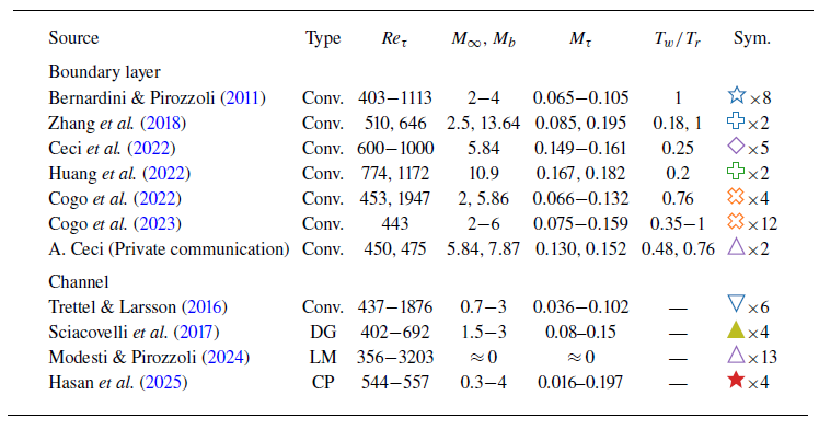
Description of the 35 boundary layer and 27 channel flow cases used in this paper. Here, $\textit{Re}_\tau = \rho _w u_\tau \delta /\mu _w$ is the friction Reynolds number based on the boundary layer thickness ( $\delta$ ) or the channel half-height ( $h$ ), $M_{\infty } = U_\infty / c_\infty$ is the free-stream Mach number (for boundary layers), $M_{b} = U_b / c_w$ is the bulk Mach number (for channels), and $M_{\tau } = u_\tau / c_w$ is the wall friction Mach number, $U_\infty$ , $U_b$ and $u_\tau$ denote the free-stream, bulk and friction velocities, respectively, $c_\infty$ and $c_w$ denote the speed of sound in the free-stream and at the wall, respectively, $T_w/T_r$ is the wall-cooling parameter, with $T_r$ being the adiabatic temperature. ‘Conv.’ indicates the conventional ideal gas cases, while ‘DG’ refers to the dense gas (supercritical) cases. Also, ‘LM’ denotes the low-Mach-number variable-property cases, in which mean property variations are induced by adding volumetric heat sources to the energy equation. Because these cases have very low Mach numbers, they are unaffected by intrinsic compressibility effects, thereby isolating variable-property effects. Finally, ‘CP’ represents constant-property high-Mach-number cases, where viscous-heating-induced mean property variations are balanced by volumetric heat sources such that the mean properties remain approximately constant throughout the domain. These cases thus isolate intrinsic compressibility effects. Finally, note that low-Reynolds-number cases in which $\textit{Re}_\tau ^*$ drops below 300 anywhere in the domain are excluded.

Figure 1.

Semi-locally scaled streamwise turbulent peak intensity, i.e. ${\widetilde {u^{\prime \prime }u^{\prime \prime }}}_p^* = \overline {\rho u^{\prime \prime }u^{\prime \prime }}_p/\tau _w$ as a function of (a) $\textit{Re}_\tau$ and (b) $\textit{Re}_\tau ^*$ taken at the peak location ( $y^*=15$ ), for the low-Mach-number variable-property cases of Modesti & Pirozzoli (Reference Modesti and Pirozzoli2024). The black curve corresponds to the fit proposed in Chen & Sreenivasan (Reference Chen and Sreenivasan2022) for incompressible flows.

To assess the correct Reynolds number that accounts for variable-property effects on wall shear stress fluctuations, and hence the peak intensity, we analyse the low-Mach-number variable-property cases of Modesti & Pirozzoli (Reference Modesti and Pirozzoli2024) described in table 1. These cases are essentially free of intrinsic compressibility effects, and therefore quantify variable-property effects. For these cases, we have computed the wall shear stress fluctuations using the interpolation technique in Smits et al. (Reference Smits, Hultmark, Lee, Pirozzoli and Wu2021), and we observed that these fluctuations scale with $\textit{Re}_\tau$ , and approximately follow the relation in Chen & Sreenivasan (Reference Chen and Sreenivasan2021), i.e. $0.25-0.42\, \textit{Re}_\tau ^{-1/4}$ (not shown). Following the discussion presented above, this implies that the peak intensity should also scale with $\textit{Re}_\tau$ . This is verified in figure 1, which shows the semi-locally scaled peak intensity ${\widetilde {u^{\prime \prime }u^{\prime \prime }}}_p^*$ as a function of $\textit{Re}_\tau$ and $\textit{Re}_\tau ^*$ taken at the peak location, i.e. $\textit{Re}_\tau ^*(y^*=15)$ . Clearly, the spread in the data with respect to the fit from Chen & Sreenivasan (Reference Chen and Sreenivasan2022) is lower for $\textit{Re}_\tau$ than for $\textit{Re}_\tau ^*(y^*=15)$ . Note that since these cases are at negligible Mach numbers, their peak intensity is a direct measure of the leading-order term in the expansion series, i.e. ${\widetilde {u_0^{\prime \prime }u_0^{\prime \prime }}}_p^*$ .

Even though $\textit{Re}_\tau$ is a better choice than the Reynolds number at the peak location, there is still some spread in the data around the curve fit (see figure 1 a). This spread is mainly attributed to the effects associated with the gradients in the semi-local Reynolds number (Patel et al. Reference Patel, Peeters, Boersma and Pecnik2015), which will be neglected here.

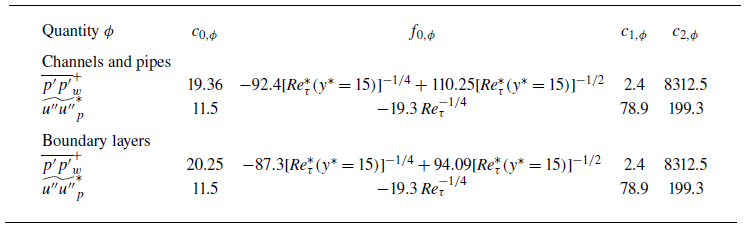
Finally, with these choices of the Reynolds numbers, we model the leading-order terms in (2.6) and (2.7) as described in table 2.

Table 2.

The constants and functions in (2.6) and (2.7), i.e. $\phi = c_{0,\phi } + f_{0,\phi } + c_{1,\phi } M_\tau ^2 + c_{2,\phi } M_\tau ^4$ (neglecting higher-order terms). The constant $c_{0,\phi }$ and the function $f_{0,\phi }$ are taken from Chen & Sreenivasan (Reference Chen and Sreenivasan2022), as discussed in § 2.1. The constants $c_{1,\phi }$ and $c_{2,\phi }$ are calibrated based on the constant-property high-Mach-number cases (Hasan et al. Reference Hasan, Costa, Larsson, Pirozzoli and Pecnik2025), as discussed in § 2.2.

2.2. Intrinsic compressibility effects

We now determine the higher-order constants in (2.6) and (2.7) using the constant-property high-Mach-number cases of Hasan et al. (Reference Hasan, Costa, Larsson, Pirozzoli and Pecnik2025), designed to isolate intrinsic compressibility effects (see table 1).

Let us first focus on wall-pressure r.m.s. To obtain the constants, we first subtract the variable-property contribution $c_{0,\phi }+f_{0,\phi }$ (see table 2) from the total $\overline {p^{\prime }p^{\prime }}_w^+$ taken from the DNS. Next, we plot this difference – which signifies the contribution by intrinsic compressibility effects – as a function of the expansion parameter $\epsilon = M_\tau$ in figure 2(a) for the four constant-property cases (denoted by red stars). Fitting a curve of the form $ M_\tau ^2 c_{1,p} + M_\tau ^4 c_{2,p}$ (neglecting higher-order terms) to these cases, we obtain $c_{1,p} = 2.4$ and $ c_{2,p} =8312.5$ ; see the black curve in figure 2(a).

Figure 2.

Contribution by intrinsic compressibility effects to (a) wall-pressure variance and (b) the peak streamwise turbulence intensity as a function of $M_\tau$ for a wide range of channels and boundary layers described in table 1. The black curves in (a) and (b) correspond to $c_{1,\phi } M_\tau ^2 + c_{2,\phi } M_\tau ^4$ , where $c_{1,\phi }$ and $c_{2,\phi }$ are reported in table 2, and $\phi$ represents wall-pressure r.m.s. or the peak intensity. These coefficients are calibrated using the constant-property cases in table 1 (red stars). The grey curve in (a) corresponds to $c_{1,p} M_\tau ^2 + c_{2,p} M_\tau ^4$ , where the coefficients $c_{1,p}=-66.9$ and $c_{2,p}=13148.7$ are obtained using the turbulent boundary layer cases listed in table 1. The insets show the intrinsic compressibility contribution as a function of $\sqrt {\tau _w/\bar p}$ . The grey symbols signify ideal gas air cases for which $\sqrt {\tau _w/\bar p} = \sqrt {1.4} M_\tau$ , and the coloured symbols represent the dense gas cases of Sciacovelli et al. (Reference Sciacovelli, Cinnella and Gloerfelt2017).

Figure 2(a) also plots the intrinsic compressibility contribution for several boundary layer and channel flow cases in the literature, as listed in table 1. Despite the fact that these cases are at different Reynolds numbers, and possess different distributions of mean properties, a majority of the cases follow the curve fit set by the constant-property cases quite well. This corroborates the assumption that we made regarding neglecting the coupling terms earlier in this section.

However, there are some exceptions. First, for the boundary layer cases of Huang, Duan & Choudhari (Reference Huang, Duan and Choudhari2022), represented by a green plus, the deviation from the curve fit is quite high. This could be due to the simplifications that we made in the analysis. It is also possible that the intrinsic compressibility contribution to wall-pressure r.m.s. differs in boundary layers compared to channels. Thus the coefficients ( $c_{1,p}$ and $c_{2,p}$ ) tuned based on the constant-property channels might not be accurate for boundary layers. Refining these coefficients for boundary layers would require constant-property high-Mach-number boundary layer simulations, which is deferred to future work. Nevertheless, in figure 2(a), we show the grey curve obtained using the conventional turbulent boundary layer cases listed in table 1. As expected, this curve aligns more closely with the green plus symbols.

Second, the dense gas cases of Sciacovelli et al. (Reference Sciacovelli, Cinnella and Gloerfelt2017) at high Mach numbers depict extremely high wall-pressure fluctuations. This is due to the proximity of these cases to the Widom line (the curve that marks the maximum of the specific heat at constant pressure, above the critical point). In this region, small pressure fluctuations can cause large density fluctuations, which in turn intensify pressure fluctuations through the source terms. Such an effect is due to the complexity of the equation of state, and is thus not accounted for in the present scaling model.

Repeating the same analysis for the peak of streamwise turbulence intensity, we get $c_{1,u} = 78.9$ and $ c_{2,u} = 199.3$ . Figure 2(b) shows the intrinsic compressibility contribution towards the peak intensity for the constant- and variable-property cases listed in table 1, along with the curve fit with tuned constants. Clearly, a majority of the cases follow the curve, corroborating that the coupling effects are small.

The insets in figure 2 show the intrinsic compressibility contributions to the wall-pressure r.m.s. and the peak intensity as functions of $\sqrt {\tau _w/\bar p}$ – the form that $\epsilon$ would take if $\bar p$ were chosen as the thermodynamic pressure scale. For the ideal gas air cases (shown in grey symbols), $\sqrt {\tau _w/\bar p}$ quantifies intrinsic compressibility effects as effectively as $M_\tau$ (main figure 2, discussed earlier), since $\sqrt {\tau _w/\bar p} \approx \gamma M_\tau$ , with $\gamma =1.4$ for these cases. However, for the dense gas cases of Sciacovelli et al. (Reference Sciacovelli, Cinnella and Gloerfelt2017) (shown in coloured symbols), the characterisation of intrinsic compressibility effects deteriorates for both wall pressure and the peak when $\sqrt {\tau _w/\bar p}$ is used instead of $M_\tau$ . These observations support our choice made in this section of using $\bar \rho \bar c^2$ as the relevant thermodynamic scale of pressure rather than $\bar p$ . This is further supported by the observation that for the dense gas cases, the upward shift in the logarithmic mean velocity profiles due to intrinsic compressibility effects (Hasan et al. Reference Hasan, Larsson, Pirozzoli and Pecnik2023) is well quantified in terms of $M_\tau$ , instead of $\sqrt {\tau _w/\bar p}$ (not shown).

Finally, it is interesting to note that for wall pressure, most of the intrinsic compressibility contribution comes from the quartic term $M_\tau ^4 c_{2,p}$ , while the same for the peak intensity stems from the quadratic term $M_\tau ^2 c_{1,u}$ . This is evident in figure 2, where the fitted curve appears quartic in figure 2(a) and quadratic in figure 2(b).

For wall pressure, the increase with Mach number has been attributed to the presence of travelling wave-packet-like structures in the pressure field (Yu et al. Reference Yu, Liu, Fu, Tang and Yuan2022; Zhang et al. Reference Zhang, Wan, Liu, Sun and Lu2022). These structures have been extensively studied in the literature (Yu, Xu & Pirozzoli Reference Yu, Xu and Pirozzoli2019; Tang et al. Reference Tang, Zhao, Wan and Liu2020; Gerolymos & Vallet Reference Gerolymos and Vallet2023; Yu et al. Reference Yu, Zhou, Dong, Yuan and Xu2024), although the physical mechanism underlying their genesis is still unclear. Recently, Hasan et al. (Reference Hasan, Costa, Larsson, Pirozzoli and Pecnik2025) reported that the component of dilatational velocity (also termed non-pseudo-sound) associated with these wave-packet-like structures increases with $M_\tau ^{3.3}$ , close to a quartic dependence. This likely explains the quartic increase in wall pressure observed in figure 2(a).

For the streamwise turbulence intensity, our recent study (Hasan et al. Reference Hasan, Costa, Larsson, Pirozzoli and Pecnik2025) concluded that the peak value increases due to the opposition of vortical motions by near-wall dilatational velocities. Specifically, this interaction modifies the turbulent shear stress, which in turn affects the production of streamwise turbulence intensity, thereby altering its peak value. This opposition mechanism scales with $M_\tau ^2$ , thereby explaining the quadratic increase in the peak intensity.

3. The final scaling relations

By combining the functions and constants obtained from §§ 2.1 and 2.2, we get the final scaling relations for the wall-pressure r.m.s. and the peak streamwise turbulence intensity, as reported in table 2. Using these relations, we compute errors with respect to the DNS as $ \varepsilon _{\phi } = ({\phi ^{\textit{DNS}} - \phi ^{\textit{model}}})/{\phi ^{\textit{DNS}}},$ where $\phi$ represents the wall-pressure r.m.s. or the peak intensity. We also compute the r.m.s. error across all cases as $\text{r.m.s.} = \sqrt {({1}/{N}) \sum \varepsilon _\phi ^2},$ where $N$ is the total number of cases.

Figure 3.

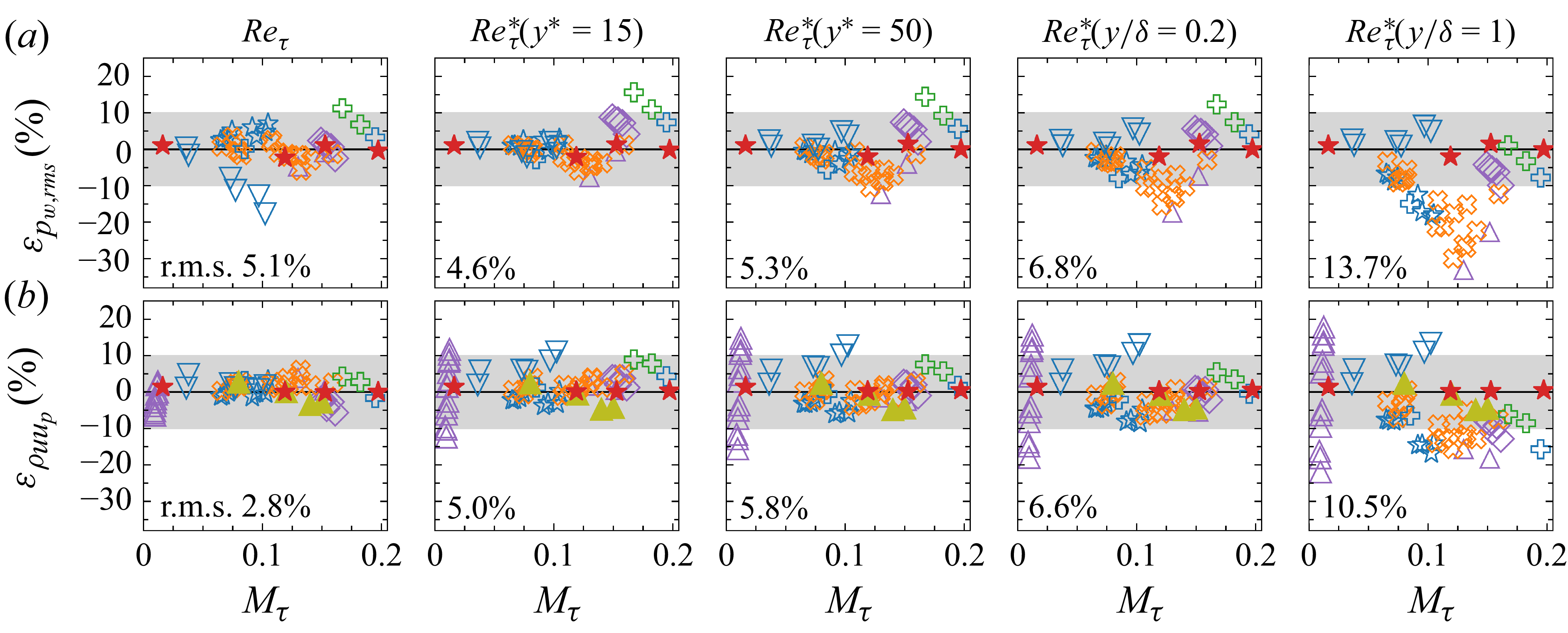
The error in the estimation of (a) wall-pressure r.m.s. and (b) the peak of streamwise turbulence intensity as a function of $M_\tau$ for the cases described in table 1. The errors are computed as discussed in the text. The different columns correspond to different Reynolds number definitions used while computing $f_{0,\phi }$ in table 2. The shaded areas represent an error margin of $\pm10\,\%$ .

To demonstrate the accuracy of our scaling relations and the appropriateness of the Reynolds number choices described in § 2.1, figure 3 presents $\varepsilon _\phi$ for the wall-pressure r.m.s. (figure 3 a) and the peak streamwise turbulence intensity (figure 3 b), for the cases listed in table 1. Note that the densegas cases were excluded from the wall-pressure error calculations. The different columns correspond to different Reynolds number definitions used while computing $f_{0,\phi }$ in table 2. Clearly, the errors associated with the Reynolds number choices made in § 2.1 – namely, $ \textit{Re}_\tau ^*(y^* = 15)$ for wall-pressure fluctuations, and $ \textit{Re}_\tau$ for the peak intensity – are relatively low when compared to those from other Reynolds number definitions, on average across all cases (compare their r.m.s. values). Furthermore, with these Reynolds number choices, a majority of the cases lie within the $\pm10\,\%$ error band.

3.1. Comparison with existing models

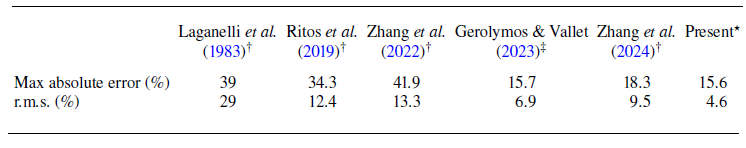
Table 3 reports the maximum absolute error and the r.m.s. error in predicting the wall-pressure r.m.s. using various models from the literature. The errors reported in table 3 were computed by applying each model to the type of flow (channel or boundary layer) for which it was originally developed. For example, the models by Laganelli et al. (Reference Laganelli, Martellucci and Shaw1983), Ritos et al. (Reference Ritos, Drikakis and Kokkinakis2019) and Zhang et al. (Reference Zhang, Wan, Liu, Sun and Lu2022, Reference Zhang, Wan, Sun and Lu2024) were applied exclusively to conventional air-like boundary layers. In contrast, the model by Gerolymos & Vallet (Reference Gerolymos and Vallet2023) was applied to both conventional channels and boundary layers, as listed in table 1. The present model was tested on a broader set of flows, including conventional channels and boundary layers, as well as the four constant-property cases reported in table 1.

Table 3.

The maximum absolute error ( $L_\infty$ norm) and the r.m.s. error ( $L_2$ norm, defined in the main text) for various wall-pressure r.m.s. models available in the literature. The models marked with $\dagger$ have been applied exclusively to conventional (ideal gas air) boundary layers, for which they were originally developed. The model marked with $\ddagger$ has been tested on both conventional channels and boundary layers. Finally, the present model, marked by $\star$ , has been applied to a broader set of flows, including conventional channels and boundary layers, as well as the four constant-property cases reported in Hasan et al. (Reference Hasan, Costa, Larsson, Pirozzoli and Pecnik2025).

As seen, the Laganelli family of models (Laganelli et al. Reference Laganelli, Martellucci and Shaw1983; Ritos et al. Reference Ritos, Drikakis and Kokkinakis2019; Zhang et al. Reference Zhang, Wan, Liu, Sun and Lu2022) yields relatively high error values, with r.m.s. error exceeding 12 %. The model proposed by Zhang et al. (Reference Zhang, Wan, Sun and Lu2024) achieves a better accuracy, with r.m.s. error 9.5 %, despite not explicitly accounting for Reynolds number or wall-cooling effects. Among the models available in the literature, the best performance is observed for the model by Gerolymos & Vallet (Reference Gerolymos and Vallet2023), which achieves r.m.s. error 6.9 %. However, this value is still high, primarily due to significant errors incurred in predicting high-Mach-number boundary layers. The present model shows improved performance over existing approaches, with the lowest r.m.s. error 4.6 %.

Finally, for the streamwise turbulence intensity peak, using the proposed relation results in maximum absolute error 6.8 % and r.m.s. error 2.8 %. These values could not be compared to those obtained from other models in the literature as, to the best of our knowledge, there are currently no models available that predict this quantity in compressible flows.

4. Summary

In this paper, we have proposed scaling relations for the wall-pressure root mean square (r.m.s.) and the streamwise turbulence intensity peak, and tested them across a wide range of turbulent channel and boundary layer cases from the literature. These relations were developed by expressing these quantities as an expansion series in terms of the friction Mach number $M_\tau$ . The first term in this series accounts for Reynolds number and variable-property effects, whereas the higher-order terms primarily capture intrinsic compressibility effects.

To model the leading-order term, we used the same expressions as proposed for incompressible flows, with an effective value of the semi-local Reynolds number that incorporates variable-property effects. For wall-pressure r.m.s, this value was found to be the Reynolds number defined in the buffer layer (at $y^*=15$ ), whereas for the peak streamwise intensity, we found the effective value to be the wall $\textit{Re}_\tau$ .

We model the higher-order correlations in the series as constants, whose values are found based on our constant-property high-Mach-number cases representative of intrinsic compressibility effects (Hasan et al. Reference Hasan, Costa, Larsson, Pirozzoli and Pecnik2025). Modelling these correlations as simple constants implies that any coupling between Reynolds number, variable-property and intrinsic compressibility effects is small – an assumption that was verified a posteriori using the available data.

Finally, an additional key finding has been noted: based on the dense gas (non-ideal) cases of Sciacovelli et al. (Reference Sciacovelli, Cinnella and Gloerfelt2017), we confirm that $\bar \rho \bar c^2$ is a more appropriate thermodynamic pressure scale than the mean pressure $\bar p$ , supporting the choice of expressing the expansion series in terms of $M_\tau$ .

We recommend the following for future work. (i) The proposed scaling approach should be tested for other turbulence quantities. (ii) The coupling effects neglected here should be explicitly quantified using a novel set of cases. For instance, to study the coupling between Reynolds number and intrinsic compressibility effects, one could simulate a similar set of constant-property, high-Mach-number cases as in Hasan et al. (Reference Hasan, Costa, Larsson, Pirozzoli and Pecnik2025), but at varying Reynolds numbers. Similarly, to study the coupling between variable-property and intrinsic compressibility effects, one could simulate cases with matching Reynolds numbers and mean property distributions but at varying Mach numbers (Lele Reference Lele1994). (iii) Constant-property, high-Mach-number compressible boundary layers should be simulated to investigate how the intrinsic compressibility contribution to wall-pressure r.m.s. differs from that in channel flows. This could shed more light on why the curve in figure 2(a), fitted based on channels, is not quite accurate for some boundary layers.