





1 Introduction
As a promising reaction for energetic
$\alpha$
 particle generation, proton–boron (
${\mathrm{p}}^{11}\mathrm{B}$
particle generation, proton–boron (
${\mathrm{p}}^{11}\mathrm{B}$
 ) fusion has attracted significant attention in recent years. Such fusion is also interesting from a fundamental point of view. Unlike traditional deuterium–tritium fusion, the
${\mathrm{p}}^{11}\mathrm{B}$
) fusion has attracted significant attention in recent years. Such fusion is also interesting from a fundamental point of view. Unlike traditional deuterium–tritium fusion, the
${\mathrm{p}}^{11}\mathrm{B}$
 reaction primarily produces
$\alpha$
reaction primarily produces
$\alpha$
 particles instead of neutrons, thereby minimizing energy loss and mitigating radiation hazards associated with neutron emission[
Reference Rostoker, Binderbauer and Monkhorst
1
,
Reference Kulcinski and Santarius
2
]. An additional advantage of the
${\mathrm{p}}^{11}\mathrm{B}$
particles instead of neutrons, thereby minimizing energy loss and mitigating radiation hazards associated with neutron emission[
Reference Rostoker, Binderbauer and Monkhorst
1
,
Reference Kulcinski and Santarius
2
]. An additional advantage of the
${\mathrm{p}}^{11}\mathrm{B}$
 reaction lies in the use of
${}^{11}\mathrm{B}$
reaction lies in the use of
${}^{11}\mathrm{B}$
 , a stable and naturally abundant element on Earth[
Reference Moreau
3
,
Reference Tentori and Belloni
4
]. The
$\alpha$
, a stable and naturally abundant element on Earth[
Reference Moreau
3
,
Reference Tentori and Belloni
4
]. The
$\alpha$
 particles generated in this reaction offer a wide range of potential applications, including cancer therapy[
Reference Yoon, Jung and Suh
5
,
Reference Cirrone, Manti, Margarone, Petringa, Giuffrida, Minopoli, Picciotto, Russo, Cammarata, Pisciotta, Perozziello, Romano, Marchese, Milluzzo, Scuderi, Cuttone and Korn
6
], material irradiation[
Reference Petringa, Cirrone, Caliri, Cuttone, Giuffrida, Larosa, Manna, Manti, Marchese, Marchetta, Margarone, Milluzzo, Picciotto, Romano, Romano, Russo, Russo, Santonocito and Scuderi
7
] and medical radioisotope production[
Reference Qaim, Spahn, Scholten and Neumaier
8
,
Reference Szkliniarz, Sitarz, Walczak, Jastrzębski, Bilewicz, Choiński, Jakubowski, Majkowska, Stolarz, Trzcińska and Zipper
9
]. Consequently, achieving a high yield of
$\alpha$
particles generated in this reaction offer a wide range of potential applications, including cancer therapy[
Reference Yoon, Jung and Suh
5
,
Reference Cirrone, Manti, Margarone, Petringa, Giuffrida, Minopoli, Picciotto, Russo, Cammarata, Pisciotta, Perozziello, Romano, Marchese, Milluzzo, Scuderi, Cuttone and Korn
6
], material irradiation[
Reference Petringa, Cirrone, Caliri, Cuttone, Giuffrida, Larosa, Manna, Manti, Marchese, Marchetta, Margarone, Milluzzo, Picciotto, Romano, Romano, Russo, Russo, Santonocito and Scuderi
7
] and medical radioisotope production[
Reference Qaim, Spahn, Scholten and Neumaier
8
,
Reference Szkliniarz, Sitarz, Walczak, Jastrzębski, Bilewicz, Choiński, Jakubowski, Majkowska, Stolarz, Trzcińska and Zipper
9
]. Consequently, achieving a high yield of
$\alpha$
 particle generation is of significant importance.
Short-pulse high-intensity lasers are widely used to induce
${\mathrm{p}}^{11}\mathrm{B}$
 fusion reaction[
Reference Daido, Nishiuchi and Pirozhkov
10
–
Reference Qin, Luo, Lan and Wang
14
]. In recent years, the
${\mathrm{p}}^{11}\mathrm{B}$
fusion reaction[
Reference Daido, Nishiuchi and Pirozhkov
10
–
Reference Qin, Luo, Lan and Wang
14
]. In recent years, the
${\mathrm{p}}^{11}\mathrm{B}$
 reaction in laser-generated plasmas has garnered significant attention from the research community[
Reference Zhang, Zhang, Dong, Fang, Gu, Dai, Qi, Deng, Zhang, Yang, Lu, Huang, Zhou, Wu, Zhou, Liu, Zhang, Li, Zhao, Yuan, Wang and Li
15
–
Reference Tosca, Molloy, McNamee, Pleskunov, Protsak, Biliak, Nikitin, Kousal, Krtouš, Hanyková, Hanuš, Biederman, Foster, Nersisyan, Martin, Ho, Macková, Mikšová, Borghesi, Kar, Istokskaia, Levy, Picciotto, Giuffrida, Margarone and Choukourov
17
]. The concept of employing either intense laser pulses or laser-accelerated proton beams to irradiate boron targets so as to generate the
${\mathrm{p}}^{11}\mathrm{B}$
reaction in laser-generated plasmas has garnered significant attention from the research community[
Reference Zhang, Zhang, Dong, Fang, Gu, Dai, Qi, Deng, Zhang, Yang, Lu, Huang, Zhou, Wu, Zhou, Liu, Zhang, Li, Zhao, Yuan, Wang and Li
15
–
Reference Tosca, Molloy, McNamee, Pleskunov, Protsak, Biliak, Nikitin, Kousal, Krtouš, Hanyková, Hanuš, Biederman, Foster, Nersisyan, Martin, Ho, Macková, Mikšová, Borghesi, Kar, Istokskaia, Levy, Picciotto, Giuffrida, Margarone and Choukourov
17
]. The concept of employing either intense laser pulses or laser-accelerated proton beams to irradiate boron targets so as to generate the
${\mathrm{p}}^{11}\mathrm{B}$
 fusion has become increasingly attractive[
Reference Belyaev, Matafonov, Vinogradov, Krainov, Lisitsa, Roussetski, Ignatyev and Andrianov
18
–
Reference Huault, Carrière, Larreur, Nicolai, Raffestin, Singappuli, D’Humieres, Dubresson, Batani, Cipriani, Filippi, Scisciò, Verona, Giuffrida, Kantarelou, Stancek, Boudjema, Lera, Pérez-Hernández, Volpe, Fìrias, Bonasera, Rodrigues, Ramìrez Chavez, Consoli and Batani
30
]. Since the first experiments in 2005, which reported yields of approximately
${10}^5\ \mathrm{sr}^{-1}$
fusion has become increasingly attractive[
Reference Belyaev, Matafonov, Vinogradov, Krainov, Lisitsa, Roussetski, Ignatyev and Andrianov
18
–
Reference Huault, Carrière, Larreur, Nicolai, Raffestin, Singappuli, D’Humieres, Dubresson, Batani, Cipriani, Filippi, Scisciò, Verona, Giuffrida, Kantarelou, Stancek, Boudjema, Lera, Pérez-Hernández, Volpe, Fìrias, Bonasera, Rodrigues, Ramìrez Chavez, Consoli and Batani
30
]. Since the first experiments in 2005, which reported yields of approximately
${10}^5\ \mathrm{sr}^{-1}$
 [
Reference Belyaev, Matafonov, Vinogradov, Krainov, Lisitsa, Roussetski, Ignatyev and Andrianov
18
], notable advancements have been realized, with extremely high yields reaching up to
${10}^{10}\ \mathrm{sr}^{-1}$
[
Reference Belyaev, Matafonov, Vinogradov, Krainov, Lisitsa, Roussetski, Ignatyev and Andrianov
18
], notable advancements have been realized, with extremely high yields reaching up to
${10}^{10}\ \mathrm{sr}^{-1}$
 in 2024[
Reference Wei, Zhang, Deng, Qi, Xu, Liu, Zhang, Li, Xu, Hoffmann, Fan, Wang, Wang, Teng, Cui, Lu, Yang, Gu, Zhao, Liu, Xie, Cao, Ren, Zhou and Zhao
28
]. In addition, Labaune et al.
[
Reference Labaune, Baccou, Depierreux, Goyon, Loisel, Yahia and Rafelski
19
] demonstrated experimentally that a hot plasma can significantly enhance
$\alpha$
in 2024[
Reference Wei, Zhang, Deng, Qi, Xu, Liu, Zhang, Li, Xu, Hoffmann, Fan, Wang, Wang, Teng, Cui, Lu, Yang, Gu, Zhao, Liu, Xie, Cao, Ren, Zhou and Zhao
28
]. In addition, Labaune et al.
[
Reference Labaune, Baccou, Depierreux, Goyon, Loisel, Yahia and Rafelski
19
] demonstrated experimentally that a hot plasma can significantly enhance
$\alpha$
 particle yields. In their study, a boron plasma, produced by a nanosecond laser, generated nearly two orders of magnitude more
$\alpha$
particle yields. In their study, a boron plasma, produced by a nanosecond laser, generated nearly two orders of magnitude more
$\alpha$
 particles than a solid boron target when both targets were irradiated by a picosecond laser-accelerated proton beam. However, the underlying physical mechanisms governing the interaction between proton beams and boron targets are still poorly understood. These mechanisms are strongly influenced by factors such as proton beam intensity, boron plasma conditions (e.g., temperature, density and composition) and the physical state of the boron (solid or plasma), all of which critically affect the
${\mathrm{p}}^{11}\mathrm{B}$
particles than a solid boron target when both targets were irradiated by a picosecond laser-accelerated proton beam. However, the underlying physical mechanisms governing the interaction between proton beams and boron targets are still poorly understood. These mechanisms are strongly influenced by factors such as proton beam intensity, boron plasma conditions (e.g., temperature, density and composition) and the physical state of the boron (solid or plasma), all of which critically affect the
${\mathrm{p}}^{11}\mathrm{B}$
 reaction and the following
$\alpha$
reaction and the following
$\alpha$
 particle production. To better understand these dynamics, further experimental and numerical investigations are required to elucidate the complicated processes involving the
${\mathrm{p}}^{11}\mathrm{B}$
particle production. To better understand these dynamics, further experimental and numerical investigations are required to elucidate the complicated processes involving the
${\mathrm{p}}^{11}\mathrm{B}$
 reaction under dense plasma and non-thermal conditions.
With the development of the structured target fabrication technique[
Reference Kulcsar, AlMawlawi, Budnik, Herman, Moskovits, Zhao and Marjoribanks
31
–
Reference Hollinger, Wang, Wang, Moreau, Capeluto, Song, Rockwood, Bayarsaikhan, Kaymak, Pukhov, Shlyaptsev and Rocca
34
], laser interaction with nanowire arrays (NWAs) has been widely used in the research of electron[
Reference Khaghani, Lobet, Borm, Burr, Gärtner, Gremillet, Movsesyan, Rosmej, ToimilMolares, Wagner and Neumayer
35
,
Reference Dozières, Petrov, Forestier-Colleoni, Campbell, Krushelnick, Maksimchuk, McGuffey, Kaymak, Pukhov, Capeluto, Hollinger, Shlyaptsev, Rocca and Beg
36
] and ion[
Reference Jiang, Ji, Audesirk, George, Snyder, Krygier, Poole, Willis, Daskalova, Chowdhury, Lewis, Schumacher, Pukhov, Freeman and Akli
37
–
Reference Wen, Tian, Yang, Wang, Cai and Zhu
40
] acceleration, X/
$\gamma$
 -ray emission[
Reference Zhang, Wu, Huang, Lan, Liu, Wu, Yang, Zhao, Zhu and Luo
41
–
Reference Shou, Kong, Wang, Mei, Cao, Pan, Li, Xu, Qi, Chen, Zhao, Zhao, Fu, Luo, Zhang, Yan and Ma
44
], nuclear isomers[
Reference Ma, Wang, Yang, Wang, Zhao, Li, Fu, He and Ma
45
,
Reference Yang, Spohr, Cernaianu, Doria, Ghenuche and Horný
46
] and neutron generation[
Reference Rubovič, Bonasera, Burian, Cao, Fu, Kong, Lan, Lou, Luo, Lv, Ma, Ma, Ma, Meduna, Mei, Mora, Pan, Shou, Sýkora, Veselský, Wang, Wang, Yan, Zhang, Zhao, Zhao and Žemlička
47
–
Reference Wang, Tinsley, Capeluto, Hollinger, Gautier and Rocca
50
]. NWAs have also been proved to be able to create extremely high-energy-density plasma environments and to largely improve the neutron yield compared with the planar target. In 2018, deuterated polyethylene NWAs were first reported to realize deuterium–deuterium fusion, producing a neutron yield of
${10}^6\ \mathrm{J}^{-1}$
-ray emission[
Reference Zhang, Wu, Huang, Lan, Liu, Wu, Yang, Zhao, Zhu and Luo
41
–
Reference Shou, Kong, Wang, Mei, Cao, Pan, Li, Xu, Qi, Chen, Zhao, Zhao, Fu, Luo, Zhang, Yan and Ma
44
], nuclear isomers[
Reference Ma, Wang, Yang, Wang, Zhao, Li, Fu, He and Ma
45
,
Reference Yang, Spohr, Cernaianu, Doria, Ghenuche and Horný
46
] and neutron generation[
Reference Rubovič, Bonasera, Burian, Cao, Fu, Kong, Lan, Lou, Luo, Lv, Ma, Ma, Ma, Meduna, Mei, Mora, Pan, Shou, Sýkora, Veselský, Wang, Wang, Yan, Zhang, Zhao, Zhao and Žemlička
47
–
Reference Wang, Tinsley, Capeluto, Hollinger, Gautier and Rocca
50
]. NWAs have also been proved to be able to create extremely high-energy-density plasma environments and to largely improve the neutron yield compared with the planar target. In 2018, deuterated polyethylene NWAs were first reported to realize deuterium–deuterium fusion, producing a neutron yield of
${10}^6\ \mathrm{J}^{-1}$
 [
Reference Curtis, Calvi, Tinsley, Hollinger, Kaymak, Pukhov, Wang, Rockwood, Wang, Shlyaptsev and Rocca
48
]. Later on,
${10}^7$
[
Reference Curtis, Calvi, Tinsley, Hollinger, Kaymak, Pukhov, Wang, Rockwood, Wang, Shlyaptsev and Rocca
48
]. Later on,
${10}^7$
 neutrons per shot were generated in a PW-level laser irradiating on NWAs[
Reference Curtis, Hollinger, Calvi, Wang, Huanyu, Wang, Pukhov, Kaymak, Baumann, Tinsley, Shlyaptsev and Rocca
49
]. Recent research shows that more than 70% of laser energy can be successfully absorbed by NWAs[
Reference Park, Tommasini, Shepherd, London, Bargsten, Hollinger, Capeluto, Shlyaptsev, Hill, Kaymak, Baumann, Pukhov, Cloyne, Costa, Hunter, Maricle, Moody and Rocca
51
] and a laser-compressed nanowire can induce an ultrafast Z-pinch formation, which facilitates nuclear fusion reactions, leading to an intense and short-lived neutron pulse[
Reference Wang, Geng, Zhang, Ji and Ma
52
]. Moreover, Wang et al.
[
Reference Wang, Xu, Zhang, Deng, Wang, Ma, Fu, Fan, Wang, Xu, Ji, Xu, Li, Lu, Shen, Liu, Yin, Geng, Zhang, Leng, Li and Ma
53
] launched an experimental campaign using NWAs to observe the
$\alpha$
neutrons per shot were generated in a PW-level laser irradiating on NWAs[
Reference Curtis, Hollinger, Calvi, Wang, Huanyu, Wang, Pukhov, Kaymak, Baumann, Tinsley, Shlyaptsev and Rocca
49
]. Recent research shows that more than 70% of laser energy can be successfully absorbed by NWAs[
Reference Park, Tommasini, Shepherd, London, Bargsten, Hollinger, Capeluto, Shlyaptsev, Hill, Kaymak, Baumann, Pukhov, Cloyne, Costa, Hunter, Maricle, Moody and Rocca
51
] and a laser-compressed nanowire can induce an ultrafast Z-pinch formation, which facilitates nuclear fusion reactions, leading to an intense and short-lived neutron pulse[
Reference Wang, Geng, Zhang, Ji and Ma
52
]. Moreover, Wang et al.
[
Reference Wang, Xu, Zhang, Deng, Wang, Ma, Fu, Fan, Wang, Xu, Ji, Xu, Li, Lu, Shen, Liu, Yin, Geng, Zhang, Leng, Li and Ma
53
] launched an experimental campaign using NWAs to observe the
$\alpha$
 particle generation from laser-driven
${\mathrm{p}}^{11}\mathrm{B}$
particle generation from laser-driven
${\mathrm{p}}^{11}\mathrm{B}$
 fusion. Since NWAs can maintain an appealing laser energy conversion efficiency and thus ions with higher energy can be produced, the resulting ion energy gain may be exploited to enhance fusion energy efficiency and
$\alpha$
fusion. Since NWAs can maintain an appealing laser energy conversion efficiency and thus ions with higher energy can be produced, the resulting ion energy gain may be exploited to enhance fusion energy efficiency and
$\alpha$
 particle yield in high-energy-density
${\mathrm{p}}^{11}\mathrm{B}$
particle yield in high-energy-density
${\mathrm{p}}^{11}\mathrm{B}$
 fusion plasmas, which remains an open question.
The particle-in-cell Monte Carlo (PIC-MC) approach has been established to study charged particle dynamics and collision processes in laboratory, astrophysical and fusion-relevant plasmas[
Reference He, Li, Fan, Wang, Liu, Lan, Wu and Ye
54
]. The introduction of pairwise-weighted fusion algorithms in particle-in-cell (PIC) simulations was first proposed by Higginson et al.
[
Reference Higginson, Link and Schmidt
55
], and later extended by Wu et al.
[
Reference Wu, Sheng, Yu, Fritzsche and He
56
] and Dong et al.
[
Reference Dong, Li, Xie, Chen, Zou, Luo and Yu
57
], through a relativistic fusion model implemented in the LAPINS and Smilei codes, respectively. Recent work by Ning et al.
[
Reference Ning, Liang, Wu, Liu, Liu, Hu, Sheng, Ren, Jiang, Zhao, Hoffmann and He
58
] systematically benchmarked LAPINS simulations against Labaune’s experimental configuration, demonstrating that the enhanced fusion yield primarily results from reduced proton energy loss, driven by the synergistic interplay between electron degeneracy effects and self-generated electromagnetic fields. In addition, Liu et al.
[
Reference Liu, Liu, Li, Yao, Zhou, Zhu, He and Qiao
59
] proposed an innovative mesh-type magnetic trap for
${\mathrm{p}}^{11}\mathrm{B}$
 fusion. Their results show that precise control of proton energy through collective field effects can substantially enhance fusion yields. Overall, these findings are revealing a strong nonlinear dependence of the
${\mathrm{p}}^{11}\mathrm{B}$
fusion. Their results show that precise control of proton energy through collective field effects can substantially enhance fusion yields. Overall, these findings are revealing a strong nonlinear dependence of the
${\mathrm{p}}^{11}\mathrm{B}$
 reaction yield on proton beam characteristics (particularly its energy spectrum) as well as on target parameters including target density and electron degeneracy.
In this study, we investigate, through PIC-MC simulations, the
${\mathrm{p}}^{11}\mathrm{B}$
 fusion plasma dynamics and the resulting production of
$\alpha$
fusion plasma dynamics and the resulting production of
$\alpha$
 particles in laser-irradiated NWA targets. We first develop a Monte Carlo (MC) nuclear reaction module for
${\mathrm{p}}^{11}\mathrm{B}$
particles in laser-irradiated NWA targets. We first develop a Monte Carlo (MC) nuclear reaction module for
${\mathrm{p}}^{11}\mathrm{B}$
 fusion within the EPOCH[
Reference Arber, Bennett, Brady, Lawrence-Douglas, Ramsay, Sircombe, Gillies, Evans, Schmitz, Bell and Ridgers
60
] framework, which is validated using a series of benchmark tests. We then employ this PIC-MC framework, together with Bayesian optimization (BO), to study the laser-driven
${\mathrm{p}}^{11}\mathrm{B}$
fusion within the EPOCH[
Reference Arber, Bennett, Brady, Lawrence-Douglas, Ramsay, Sircombe, Gillies, Evans, Schmitz, Bell and Ridgers
60
] framework, which is validated using a series of benchmark tests. We then employ this PIC-MC framework, together with Bayesian optimization (BO), to study the laser-driven
${\mathrm{p}}^{11}\mathrm{B}$
 fusion and
$\alpha$
fusion and
$\alpha$
 particle generation in NWA targets.
Note that BO can help to optimize the laser intensity and target configuration and then to improve the simulation efficiency. Two-dimensional (2D) PIC-MC simulation results show that the NWA target enhances the
${\mathrm{p}}^{11}\mathrm{B}$
 fusion yield by nearly two orders of magnitude compared with a planar target. This enhancement is mainly attributed to an efficient ion acceleration by sheath fields. The reminder of the paper is organized as follows. Section 2 introduces the implementation of the MC process for
${\mathrm{p}}^{11}\mathrm{B}$
fusion yield by nearly two orders of magnitude compared with a planar target. This enhancement is mainly attributed to an efficient ion acceleration by sheath fields. The reminder of the paper is organized as follows. Section 2 introduces the implementation of the MC process for
${\mathrm{p}}^{11}\mathrm{B}$
 fusion within EPOCH. Section 3 presents benchmark simulation results that validate our method. In Section 4, we employ BO to optimize key laser-target parameters and then investigate the mechanisms of enhanced fusion reaction and
$\alpha$
fusion within EPOCH. Section 3 presents benchmark simulation results that validate our method. In Section 4, we employ BO to optimize key laser-target parameters and then investigate the mechanisms of enhanced fusion reaction and
$\alpha$
 particle generation in the NWA targets. Finally, Section 5 provides a summary and outlook for future research.
2 The implementation of the
${\mathbf{p}}^{\mathbf{11}}\mathbf{B}$
 fusion module

The
${\mathrm{p}}^{11}\mathrm{B}$
 fusion reaction (p +
${}^{11}\mathrm{B}$
fusion reaction (p +
${}^{11}\mathrm{B}$ $\to$
$\to$
 3
$\alpha$
3
$\alpha$
 + 8.7 MeV) proceeds through several intermediate stages. A high-energy proton first collides with a
${}^{11}\mathrm{B}$
+ 8.7 MeV) proceeds through several intermediate stages. A high-energy proton first collides with a
${}^{11}\mathrm{B}$
 nucleus, forming an excited
${}^{12}{\mathrm{C}}^{\ast }$
nucleus, forming an excited
${}^{12}{\mathrm{C}}^{\ast }$
 intermediate state. This metastable nucleus rapidly decays into one
$\alpha$
intermediate state. This metastable nucleus rapidly decays into one
$\alpha$
 particle and an unstable
${}^8\mathrm{Be}$
particle and an unstable
${}^8\mathrm{Be}$
 nucleus, which subsequently dissociates into two additional
$\alpha$
nucleus, which subsequently dissociates into two additional
$\alpha$
 particles. The final products are three
$\alpha$
particles. The final products are three
$\alpha$
 particles, each carrying part of the total released energy. For the above
${\mathrm{p}}^{11}\mathrm{B}$
particles, each carrying part of the total released energy. For the above
${\mathrm{p}}^{11}\mathrm{B}$
 fusion and
$\alpha$
fusion and
$\alpha$
 particles generation processes, the corresponding MC module is implemented within the EPOCH framework by the following four main steps.
-
(1) Particle pairing
In each spatial cell, pairs of two macro-particles undergoing nuclear fusion are selected randomly. The pairing procedure follows the method proposed by Takizuka and Abe[ Reference Takizuka and Abe 61 ].
-
(2) Fusion probability
For each paired proton and boron macro-particles (with assigned weights), the probability of fusion within a time step
$\Delta$
 t is given by the following:

where
${n}_{\mathrm{min}}$
 is the minimum number density between two species (proton and
${}^{11}\mathrm{B}$
is the minimum number density between two species (proton and
${}^{11}\mathrm{B}$
 ),
${v}_{\mathrm{rel}}$
),
${v}_{\mathrm{rel}}$
 is their relative velocity and
${W}_{\mathrm{min}}$
is their relative velocity and
${W}_{\mathrm{min}}$
 is the minimum weight of their macro-particles[
Reference Dozières, Petrov, Forestier-Colleoni, Campbell, Krushelnick, Maksimchuk, McGuffey, Kaymak, Pukhov, Capeluto, Hollinger, Shlyaptsev, Rocca and Beg
36
]. The term
$\sigma \left({E}_i\right)$
is the minimum weight of their macro-particles[
Reference Dozières, Petrov, Forestier-Colleoni, Campbell, Krushelnick, Maksimchuk, McGuffey, Kaymak, Pukhov, Capeluto, Hollinger, Shlyaptsev, Rocca and Beg
36
]. The term
$\sigma \left({E}_i\right)$
 represents the energy-dependent fusion cross-section, which is interpolated from the EXFOR experimental database[
62
]. The specific data values and fitting methods are described in Appendix A. Based on
${P}_i$
represents the energy-dependent fusion cross-section, which is interpolated from the EXFOR experimental database[
62
]. The specific data values and fitting methods are described in Appendix A. Based on
${P}_i$
 , an MC sampling method is used to determine whether a fusion event occurs. The pseudo-code for the fusion probability calculation is presented below.

Table 1 Long description
The table is titled Fusion probability and contains the following sequential steps.
1. Compute reaction probability using the formula: P sub i equals n sub mathrm min sigma open parenthesis E sub i close parenthesis v sub mathrm rel Delta t sub mathrm min.
2. Sample random number: U in the interval open bracket 0 comma 1 close bracket.
3. Optical depth: R equals minus log open parenthesis 1 minus U close parenthesis.
4. Judge criterion: if R is less than P sub i then fusion occurs.
-
(3) Reaction channel selection
After fusion occurs, the reaction channel must be determined. In the
${\mathrm{p}}^{11}\mathrm{B}$
 fusion module, only the sequential decay pathway is considered, as it dominates the total reaction cross-section (
$\approx$
fusion module, only the sequential decay pathway is considered, as it dominates the total reaction cross-section (
$\approx$
 95%). This pathway includes two channels:
${}^{11}\mathrm{B}$
95%). This pathway includes two channels:
${}^{11}\mathrm{B}$
 (p,
${\alpha}_0$
(p,
${\alpha}_0$
 )
${}^8\mathrm{Be}$
)
${}^8\mathrm{Be}$
 and
${}^{11}\mathrm{B}$
and
${}^{11}\mathrm{B}$
 (p,
${\alpha}_1$
(p,
${\alpha}_1$
 )
${}^8\mathrm{Be}$
)
${}^8\mathrm{Be}$
 *. To identify which channel occurs, a branching ratio
${S}_i$
*. To identify which channel occurs, a branching ratio
${S}_i$
 is introduced. The pseudo-code for reaction channel selection is shown below.

Table 2 Long description
The table is titled Reaction channel selection and consists of three numbered steps.
Step 1. Calculate branching ratio. The equation is S sub i equals the fraction with numerator sigma sub 2 open parenthesis E sub i close parenthesis all over denominator sigma sub 1 open parenthesis E sub i close parenthesis plus sigma sub 2 open parenthesis E sub i close parenthesis. The text specifies that sigma sub 1 open parenthesis E sub i close parenthesis and sigma sub 2 open parenthesis E sub i close parenthesis represent the cross-section values for the reactions 11 B open parenthesis p comma alpha sub 0 close parenthesis 8 Be and 11 B open parenthesis p comma alpha sub 1 close parenthesis 8 Be star, respectively.
Step 2. Sample random number. The expression is U sub 1 is an element of the closed interval from 0 to 1.
Step 3. Reaction channel selection. This uses conditional logic. If U sub 1 is less than or equal to S sub i, then the reaction 11 B open parenthesis p comma alpha sub 1 close parenthesis 8 Be star occurs. Else, the reaction 11 B open parenthesis p comma alpha sub 0 close parenthesis 8 Be occurs.
-
(4) Fusion reaction kinematics
After the reaction channel is selected, the energies and momenta of the fusion products are calculated. In the MC
${\mathrm{p}}^{11}\mathrm{B}$
 fusion module, all fusion products are generated in the center-of-mass (COM) frame and then transformed to the simulation (S) frame. A rotation matrix is introduced to transform the coordinate system in COM space. The transformation method follows that proposed by Takizuka and Abe[
Reference Takizuka and Abe
61
]. In this section, only the computational procedures in the COM frame are described, as detailed physical discussions can be found in previous studies[
Reference Higginson, Link and Schmidt
55
]. The
${}^{11}\mathrm{B}$
fusion module, all fusion products are generated in the center-of-mass (COM) frame and then transformed to the simulation (S) frame. A rotation matrix is introduced to transform the coordinate system in COM space. The transformation method follows that proposed by Takizuka and Abe[
Reference Takizuka and Abe
61
]. In this section, only the computational procedures in the COM frame are described, as detailed physical discussions can be found in previous studies[
Reference Higginson, Link and Schmidt
55
]. The
${}^{11}\mathrm{B}$
 (p,
${\alpha}_1$
(p,
${\alpha}_1$
 )
${}^8\mathrm{Be}$
)
${}^8\mathrm{Be}$
 * channel is used as an example.
For the reaction p +
${}^{11}\mathrm{B}$ $\to$
$\to$ ${\alpha}_1$
 +
${}^8\mathrm{Be}$
+
${}^8\mathrm{Be}$
 * +
${Q}_1$
* +
${Q}_1$
 (Phase I), the released energy is
${Q}_1=5.65$
(Phase I), the released energy is
${Q}_1=5.65$
 MeV. The velocities of
${\alpha}_1$
MeV. The velocities of
${\alpha}_1$
 and
${}^8\mathrm{Be}$
and
${}^8\mathrm{Be}$
 * in the COM frame are obtained as follows:

where

with

and

where
${m}_{\mathrm{p}}$
 ,
${m}_{11_{\mathrm{B}}}$
,
${m}_{11_{\mathrm{B}}}$
 ,
${m}_{\alpha_1}$
,
${m}_{\alpha_1}$
 and
${m}_{{}^8\mathrm{Be}}{\hbox{\(\ast\)}}$
and
${m}_{{}^8\mathrm{Be}}{\hbox{\(\ast\)}}$
 are the rest mass of the proton, boron target,
${\alpha}_1$
are the rest mass of the proton, boron target,
${\alpha}_1$
 and
${}^8\mathrm{Be}$
and
${}^8\mathrm{Be}$
 *, respectively. In Equation (2),
${\theta}_{\mathrm{C}}$
*, respectively. In Equation (2),
${\theta}_{\mathrm{C}}$
 and
${\varphi}_{\mathrm{C}}$
and
${\varphi}_{\mathrm{C}}$
 denote the polar and azimuthal angles, respectively, of
${\alpha}_1$
denote the polar and azimuthal angles, respectively, of
${\alpha}_1$
 in the COM frame. The polar angle
${\theta}_{\mathrm{C}}$
in the COM frame. The polar angle
${\theta}_{\mathrm{C}}$
 is sampled according to the differential cross-section
$\sigma \left({\theta}_{\mathrm{C}}\right)$
is sampled according to the differential cross-section
$\sigma \left({\theta}_{\mathrm{C}}\right)$
 , which is interpolated from EXFOR experimental data. The azimuthal angle
${\varphi}_{\mathrm{C}}$
, which is interpolated from EXFOR experimental data. The azimuthal angle
${\varphi}_{\mathrm{C}}$
 is randomly selected from 0 to 2
$\pi$
is randomly selected from 0 to 2
$\pi$
 . The values and fitting procedure of
$\sigma \left({\theta}_{\mathrm{C}}\right)$
. The values and fitting procedure of
$\sigma \left({\theta}_{\mathrm{C}}\right)$
 are presented in Appendix A.
For the subsequent decay
${}^8\mathrm{Be}$
 *
$\to$
*
$\to$ ${\alpha}_{11}$
 +
${\alpha}_{12}$
+
${\alpha}_{12}$
 +
${Q}_2$
+
${Q}_2$
 (Phase II), the released energy is
${Q}_2$
(Phase II), the released energy is
${Q}_2$
 = 3.028 MeV. The velocities of
${\alpha}_{11}$
= 3.028 MeV. The velocities of
${\alpha}_{11}$
 and
${\alpha}_{12}$
and
${\alpha}_{12}$
 in the COM frame are derived as follows:

where

and

In Equation (6),
${\theta}_{\mathrm{C}1}$
 and
${\varphi}_{\mathrm{C}1}$
and
${\varphi}_{\mathrm{C}1}$
 denote the polar and azimuthal angles of
${\alpha}_{11}$
denote the polar and azimuthal angles of
${\alpha}_{11}$
 , respectively;
${\varphi}_{\mathrm{C}1}$
, respectively;
${\varphi}_{\mathrm{C}1}$
 is randomly chosen from 0 to 2
$\pi$
is randomly chosen from 0 to 2
$\pi$
 , while
${\theta}_{\mathrm{C}1}$
, while
${\theta}_{\mathrm{C}1}$
 is sampled according to
$\sigma \left({\theta}_{\mathrm{C}1}\right)$
is sampled according to
$\sigma \left({\theta}_{\mathrm{C}1}\right)$
 . The corresponding
$\sigma \left({\theta}_{\mathrm{C}1}\right)$
. The corresponding
$\sigma \left({\theta}_{\mathrm{C}1}\right)$
 data and fitting method are also detailed in Appendix A. The pseudo-code for calculating the fusion reaction kinematics is provided below.

Table 3 Long description
The table is titled Fusion reaction kinematics and details the angular distribution sampling for Phases I and II.
Step 1. Generate a candidate angle from a uniform distribution: theta super asterisk in the range of open bracket 0, 2 pi close bracket.
Step 2. Generate a uniform random number for the acceptance test: U sub 2 in the range of open bracket 0, 1 close bracket.
Step 3. Evaluate the differential cross-section sigma open parenthesis theta super asterisk close parenthesis at theta super asterisk. Compute the acceptance probability as follows: P sub mathrm accept equals the fraction with numerator sigma open parenthesis theta super asterisk close parenthesis all over denominator 2 pi integral from 0 to pi of sigma open parenthesis theta super asterisk close parenthesis sine open parenthesis theta super asterisk close parenthesis d open parenthesis theta super asterisk close parenthesis.
Step 4. Accept or reject the candidate angle: if U sub 2 is less than or equal to P sub mathrm accept, then accept sigma open parenthesis theta super asterisk close parenthesis; otherwise, reject it and repeat the process.
The final bullet point states: Calculate the energy and momentum of the corresponding fusion products based on the angles theta super asterisk.
The above steps complete the derivation of the kinematic process for the
${}^{11}\mathrm{B}$
 (p,
${\alpha}_1$
(p,
${\alpha}_1$
 )
${}^8\mathrm{Be}$
)
${}^8\mathrm{Be}$
 * reaction. The kinematic process of the alternative channel,
${}^{11}\mathrm{B}$
* reaction. The kinematic process of the alternative channel,
${}^{11}\mathrm{B}$
 (p,
${\alpha}_0$
(p,
${\alpha}_0$
 )
${}^8\mathrm{Be}$
)
${}^8\mathrm{Be}$
 , is analogous, differing only in the reaction energy
$Q$
, is analogous, differing only in the reaction energy
$Q$
 .
.
3 Benchmark results
3.1 Beam–target fusion
To validate the algorithm, 2D beam–target simulations were performed to analyze
$\alpha$
 particle generation from
${\mathrm{p}}^{11}\mathrm{B}$
particle generation from
${\mathrm{p}}^{11}\mathrm{B}$
 fusion reactions. The simulation domain was
$40\;\unicode{x3bc} \mathrm{m}\times 40\;\unicode{x3bc} \mathrm{m}$
fusion reactions. The simulation domain was
$40\;\unicode{x3bc} \mathrm{m}\times 40\;\unicode{x3bc} \mathrm{m}$
 , divided into
$800\times 400$
, divided into
$800\times 400$
 cells, with 50 macro-particles per cell. The time step was set to
${T}_0$
cells, with 50 macro-particles per cell. The time step was set to
${T}_0$
 = 20 fs. A cold
${}^{11}\mathrm{B}$
= 20 fs. A cold
${}^{11}\mathrm{B}$
 target with a number density of
${n}_{{}^{11}\mathrm{B}}$
target with a number density of
${n}_{{}^{11}\mathrm{B}}$
 =
$1\times {10}^{28}$
=
$1\times {10}^{28}$
 m
${}^{-3}$
m
${}^{-3}$
 was bombarded by a proton beam with a number density of
${n}_{\mathrm{p}}$
was bombarded by a proton beam with a number density of
${n}_{\mathrm{p}}$
 =
$1\times {10}^{23}$
=
$1\times {10}^{23}$
 m
${}^{-3}$
m
${}^{-3}$
 . The proton beam duration was 1 ps. The beam entered the domain from the left-hand boundary along the x-axis, within the range y = –2.5 to 2.5
$\unicode{x3bc}$
. The proton beam duration was 1 ps. The beam entered the domain from the left-hand boundary along the x-axis, within the range y = –2.5 to 2.5
$\unicode{x3bc}$
 m. A 5
$\unicode{x3bc}$
m thick boron target was located in the region 2 < x < 7
$\unicode{x3bc}$
m, extending along y = –5 to 5
$\unicode{x3bc}$
m. Periodic boundary conditions were applied to all particles to ensure accurate tracking of
$\alpha$
m. A 5
$\unicode{x3bc}$
m thick boron target was located in the region 2 < x < 7
$\unicode{x3bc}$
m, extending along y = –5 to 5
$\unicode{x3bc}$
m. Periodic boundary conditions were applied to all particles to ensure accurate tracking of
$\alpha$
 particle generation.
3.1.1 The total yield of
$\alpha$
particles

Simulations of total
$\alpha$
 particle yields were performed for three proton energies of 0.675, 1.37 and 2.64 MeV. For a thin target, the
$\alpha$
particle yields were performed for three proton energies of 0.675, 1.37 and 2.64 MeV. For a thin target, the
$\alpha$
 particle yield,
${N}_{\alpha }$
particle yield,
${N}_{\alpha }$
 , from the fusion reaction is expressed as follows:

where
${N}_{\mathrm{p}}$
 is the number of protons,
${n}_{\mathrm{B}}$
is the number of protons,
${n}_{\mathrm{B}}$
 is the density of
${}^{11}\mathrm{B}$
is the density of
${}^{11}\mathrm{B}$
 nuclei,
$d$
nuclei,
$d$
 is the target thickness and
$\sigma$
is the target thickness and
$\sigma$
 (E
${}_{\mathrm{p}}$
(E
${}_{\mathrm{p}}$
 ) is the fusion cross-section. The simulated results and theoretical predictions obtained with Equation (9) are summarized in Table 4. The deviation between them is within 4%. This discrepancy mainly arises from the non-ideal monoenergetic nature of the proton source and the minor variations introduced by the energy-dependent interpolation of the reaction cross-section during the iterative computation process.
Comparison between simulated and theoretical
$\alpha$
 particle yields for
${\mathrm{p}}^{11}\mathrm{B}$
particle yields for
${\mathrm{p}}^{11}\mathrm{B}$
 fusion reactions.

Table 4 Long description
The table is organized by Proton energy in M e V, with two primary reaction headers: 11 B open parenthesis p, alpha sub 0 close parenthesis 8 Be and 11 B open parenthesis p, alpha sub 1 close parenthesis 8 Be super asterisk. Each reaction contains four columns: Cross-section in m-squared, Simulated yield, Theoretical yield, and Deviation in percent.
* At 2.64 M e V:
- For alpha sub 0: Cross-section 5.80e minus 30, Simulated 3.34e6, Theoretical 3.26e6, Deviation 2.45 percent.
- For alpha sub 1: Cross-section 2.06e minus 29, Simulated 1.13e7, Theoretical 1.16e7, Deviation 2.59 percent.
* At 1.37 M e V:
- For alpha sub 0: Cross-section 6.56e minus 31, Simulated 2.69e5, Theoretical 2.66e5, Deviation 1.12 percent.
- For alpha sub 1: Cross-section 1.74e minus 29, Simulated 7.05e6, Theoretical 7.04e6, Deviation 0.14 percent.
* At 0.675 M e V:
- For alpha sub 0: Cross-section 4.81e minus 31, Simulated 1.42e5, Theoretical 1.37e5, Deviation 3.64 percent.
- For alpha sub 1: Cross-section 1.16e minus 28, Simulated 3.31e7, Theoretical 3.29e7, Deviation 0.06 percent.
3.1.2 The energy-angle distribution of
$\alpha$
particles

For a proton energy of
${E}_{\mathrm{p}}=0.675\;\mathrm{MeV}$
 at
${\theta}_{\alpha}^{\mathrm{lab}}=90{}^{\circ}$
at
${\theta}_{\alpha}^{\mathrm{lab}}=90{}^{\circ}$
 (Figure 1(a)), the energy spectrum of secondary
$\alpha$
(Figure 1(a)), the energy spectrum of secondary
$\alpha$
 particles shows a saddle-shaped distribution, consistent with experimental data. The
$\alpha$
particles shows a saddle-shaped distribution, consistent with experimental data. The
$\alpha$
 particles are mainly emitted in two energy groups: one centered around 4 MeV and the other near 1 MeV. The strong peak below 1 MeV observed in the experimental data (black curve), which results from elastic proton scattering, does not appear in the simulation. At
${E}_{\mathrm{p}}=1.37\;\mathrm{MeV}$
particles are mainly emitted in two energy groups: one centered around 4 MeV and the other near 1 MeV. The strong peak below 1 MeV observed in the experimental data (black curve), which results from elastic proton scattering, does not appear in the simulation. At
${E}_{\mathrm{p}}=1.37\;\mathrm{MeV}$
 (Figure 1(b)), the simulated
$\alpha$
(Figure 1(b)), the simulated
$\alpha$
 particle spectrum agrees well with the measurements, exhibiting an
${\alpha}_1$
particle spectrum agrees well with the measurements, exhibiting an
${\alpha}_1$
 peak at 5.2 MeV. Overall, the spectral distribution simulated shows good agreement with the experimental data in terms of the major energy peaks, spectral shape and an overall trend. Although full three-dimensional (3D) simulations would be required for a fully quantitative comparison of absolute particle yields and detailed angular distributions, the above agreement in these key spectral features supports the use of 2D simulations for benchmarking the underlying physical mechanisms. Figure 2 shows the angular distributions of
$\alpha$
peak at 5.2 MeV. Overall, the spectral distribution simulated shows good agreement with the experimental data in terms of the major energy peaks, spectral shape and an overall trend. Although full three-dimensional (3D) simulations would be required for a fully quantitative comparison of absolute particle yields and detailed angular distributions, the above agreement in these key spectral features supports the use of 2D simulations for benchmarking the underlying physical mechanisms. Figure 2 shows the angular distributions of
$\alpha$
 particles for
${E}_{\mathrm{p}}$
particles for
${E}_{\mathrm{p}}$
 = 2.64 MeV. The intensities of the
${\alpha}_1$
= 2.64 MeV. The intensities of the
${\alpha}_1$
 and
${\alpha}_0$
and
${\alpha}_0$
 peaks decrease with the increasing detection angle. The simulated energy range agrees well with theoretical predictions. The energies of both
${\alpha}_1$
peaks decrease with the increasing detection angle. The simulated energy range agrees well with theoretical predictions. The energies of both
${\alpha}_1$
 and
${\alpha}_0$
and
${\alpha}_0$
 particles remain nearly constant within 0°–10° and 170°–180°, respectively. Due to the difference in reaction
$Q$
particles remain nearly constant within 0°–10° and 170°–180°, respectively. Due to the difference in reaction
$Q$
 values,
${\alpha}_0$
values,
${\alpha}_0$
 particles have higher energies than
${\alpha}_1$
particles have higher energies than
${\alpha}_1$
 particles. The simulated angular-energy distribution agrees closely with reference data, confirming the validity of the current EPOCH implementation.
Spectra of the simulated
$\alpha$
 particles (red curves) compared with the experimental data (black curves) for (a)
${E}_{\mathrm{p}}$
particles (red curves) compared with the experimental data (black curves) for (a)
${E}_{\mathrm{p}}$
 = 0.675 MeV at
${\theta}_{\alpha}^{\mathrm{lab}}=90{}^{\circ}$
= 0.675 MeV at
${\theta}_{\alpha}^{\mathrm{lab}}=90{}^{\circ}$
 and (b)
${E}_{\mathrm{p}}$
and (b)
${E}_{\mathrm{p}}$
 = 1.37 MeV at
${\theta}_{\alpha}^{\mathrm{lab}}=30{}^{\circ}$
= 1.37 MeV at
${\theta}_{\alpha}^{\mathrm{lab}}=30{}^{\circ}$
 . The curves in green and blue represent the primary and the secondary
$\alpha$
. The curves in green and blue represent the primary and the secondary
$\alpha$
 particle energy spectra from the
${}^{11}\mathrm{B}{\left(\mathrm{p},{\alpha}_1\right)}^8{\mathrm{Be}}^{\ast }$
particle energy spectra from the
${}^{11}\mathrm{B}{\left(\mathrm{p},{\alpha}_1\right)}^8{\mathrm{Be}}^{\ast }$
 channel. The experimental data are from Refs. [Reference Stave, Ahmed, France, Karwowski, Mueller, Prior, Spraker and Weller63,Reference Li, Yuan, Lin, Zhang and Meng64].

Figure 1 Long description
Two panels labeled a and b show energy spectra with the x-axis as E sub alpha in M e V from 0 to 8 and the y-axis as Counts.
Panel a represents E sub p equals 0.675 M e V at theta sub alpha lab equals 90 degrees.
* A black solid line for experimental total data shows a sharp narrow peak near 0.5 M e V reaching 150 counts and a broad peak centered near 4.2 M e V reaching approximately 110 counts.
* A red stepped line for simulated total data follows the broad peak but lacks the sharp low-energy peak.
* A green dotted line for primary alpha particles forms a narrow peak within the broad peak at 4.2 M e V.
* A blue dashed line for secondary alpha particles forms a wider base under the broad peak from 3.5 to 5.0 M e V and a low plateau from 0 to 3.5 M e V.
Panel b represents E sub p equals 1.37 M e V at theta sub alpha lab equals 30 degrees.
* The black experimental line shows a broad peak from 0 to 2 M e V and a higher peak near 5.2 M e V reaching 150 counts.
* The red simulated line shows a high-intensity stepped peak at 0.5 M e V and another at 5.2 M e V.
* The green dotted primary alpha line contributes to the sharp peak at 5.2 M e V.
* The blue dashed secondary alpha line matches the simulated data in the 0 to 4 M e V range and forms a lower shoulder on the 5.2 M e V peak.
The angular distributions of the
$\alpha$
 particle beams with their energies for 2.64 MeV. The theoretical distributions for
${\alpha}_1$
particle beams with their energies for 2.64 MeV. The theoretical distributions for
${\alpha}_1$
 and
${\alpha}_0$
and
${\alpha}_0$
 emissions were calculated according to Equation (2). As mentioned above,
${\alpha}_1$
emissions were calculated according to Equation (2). As mentioned above,
${\alpha}_1$
 and
${\alpha}_0$
and
${\alpha}_0$
 are produced by
${}^{11}\mathrm{B}{\left(\mathrm{p},{\alpha}_1\right)}^8{\mathrm{Be}}^{\ast }$
are produced by
${}^{11}\mathrm{B}{\left(\mathrm{p},{\alpha}_1\right)}^8{\mathrm{Be}}^{\ast }$
 and
${}^{11}\mathrm{B}{\left(\mathrm{p},{\alpha}_0\right)}^8\mathrm{Be}$
and
${}^{11}\mathrm{B}{\left(\mathrm{p},{\alpha}_0\right)}^8\mathrm{Be}$
 reactions, respectively.

Figure 2 Long description
A two-dimensional heat map plot.
* The horizontal x-axis represents energy E sub alpha in M e V, ranging from 0 to 9.
* The vertical y-axis represents the angle theta in degrees, ranging from 0 to 180.
* A color bar on the right indicates intensity d N sub alpha over d E d theta, ranging from 0 in white to 0.2 in dark red.
* In the top-left corner, text indicates t equals 70 T sub 0.
* The plot contains scattered blue data points forming vertical bands.
* A black dashed line labeled theory alpha sub 1 starts at approximately 4.2 M e V at 180 degrees, curves rightward to a peak near 6.8 M e V at 0 degrees, following a dense blue data ridge.
* A pink dashed line labeled theory alpha sub 0 starts at approximately 6 M e V at 180 degrees and curves rightward to approximately 9 M e V at 0 degrees, following a lighter data ridge.
* Lower energy regions between 0 and 4 M e V show diffuse vertical bands of low-intensity blue data.
3.2 Thermonuclear fusion
To compare with theoretical predictions, we performed numerical simulations in a 2D domain. The simulation box had dimensions of
${L}_x=5\kern0.22em \unicode{x3bc} \mathrm{m}$
 and
${L}_y=2\kern0.22em \unicode{x3bc} \mathrm{m}$
and
${L}_y=2\kern0.22em \unicode{x3bc} \mathrm{m}$
 . It was divided into
$500\times 200$
. It was divided into
$500\times 200$
 cells, with each cell containing an equal number of protons and
${}^{11}\mathrm{B}$
cells, with each cell containing an equal number of protons and
${}^{11}\mathrm{B}$
 ions. The ion number density was
${10}^{25}\kern0.1em {\mathrm{m}}^{-3}$
ions. The ion number density was
${10}^{25}\kern0.1em {\mathrm{m}}^{-3}$
 . The simulation time was set to
$t=100\kern0.22em \mathrm{fs}$
. The simulation time was set to
$t=100\kern0.22em \mathrm{fs}$
 under different temperature conditions. The initial ion velocities followed the Maxwell–Boltzmann distribution. The theoretical fusion reaction rate is expressed as
$\left\langle \sigma v\right\rangle ={\left(\frac{8}{\pi \mu}\right)}^{1/2}\frac{1}{(kT)^{3/2}}{\int}_0^{\infty } E\sigma (E)\exp \left(-\frac{E}{kT}\right)\mathrm{d}E$
under different temperature conditions. The initial ion velocities followed the Maxwell–Boltzmann distribution. The theoretical fusion reaction rate is expressed as
$\left\langle \sigma v\right\rangle ={\left(\frac{8}{\pi \mu}\right)}^{1/2}\frac{1}{(kT)^{3/2}}{\int}_0^{\infty } E\sigma (E)\exp \left(-\frac{E}{kT}\right)\mathrm{d}E$
 [
Reference Tentori and Belloni
65
]. The reaction rate obtained from simulations is calculated as
$\left\langle \sigma v\right\rangle ={N}_{\alpha }/{n}_{\mathrm{p}}{n}_{\mathrm{B}} tV$
[
Reference Tentori and Belloni
65
]. The reaction rate obtained from simulations is calculated as
$\left\langle \sigma v\right\rangle ={N}_{\alpha }/{n}_{\mathrm{p}}{n}_{\mathrm{B}} tV$
 , where
${N}_{\alpha }$
, where
${N}_{\alpha }$
 is the number of
$\alpha$
is the number of
$\alpha$
 particles and
$V$
particles and
$V$
 is the target volume. Periodic boundary conditions were applied. As a result, the ion velocity distribution remained nearly unchanged during the simulation, and the fusion reaction rate
$\left\langle \sigma v\right\rangle$
is the target volume. Periodic boundary conditions were applied. As a result, the ion velocity distribution remained nearly unchanged during the simulation, and the fusion reaction rate
$\left\langle \sigma v\right\rangle$
 stayed approximately constant over time. This allows a direct comparison between theoretical and simulated results to evaluate the reliability of the calculated reaction rates. Figure 3 shows the fusion reaction rates at different temperatures, which exhibit close agreement between the simulation and theoretical predictions.
Validation of the MC
${\mathrm{p}}^{11}\mathrm{B}$
 fusion module implemented within the EPOCH framework. The
${\mathrm{p}}^{11}\mathrm{B}$
fusion module implemented within the EPOCH framework. The
${\mathrm{p}}^{11}\mathrm{B}$
 fusion reaction rates are calculated within a box with the sensitivity to temperature variations.

4 Results and discussion
4.1 Laser-driven NWA configuration
With the
${\mathrm{p}}^{11}\mathrm{B}$
 nuclear reaction module implemented, we performed self-consistent 2D PIC-MC simulations for femtosecond (fs) laser-driven NWA targets. A schematic of the simulation setup is shown in Figure 4. The simulation box size was 35
$\unicode{x3bc}$
m
$\times$
nuclear reaction module implemented, we performed self-consistent 2D PIC-MC simulations for femtosecond (fs) laser-driven NWA targets. A schematic of the simulation setup is shown in Figure 4. The simulation box size was 35
$\unicode{x3bc}$
m
$\times$
 10
$\unicode{x3bc}$
m, divided into
$3500\times 1000$
10
$\unicode{x3bc}$
m, divided into
$3500\times 1000$
 cells in the
$x$
cells in the
$x$
 and
$y$
and
$y$
 directions, respectively. The laser wavelength was
${\lambda}_0=0.8\;\unicode{x3bc} \mathrm{m}$
directions, respectively. The laser wavelength was
${\lambda}_0=0.8\;\unicode{x3bc} \mathrm{m}$
 . A linearly
$y$
. A linearly
$y$
 polarized laser pulse with a Gaussian profile propagated along the
$x$
polarized laser pulse with a Gaussian profile propagated along the
$x$
 -axis from the left-hand boundary and was normally incident on the NWA targets. The pulse duration was
${\tau}_0$
-axis from the left-hand boundary and was normally incident on the NWA targets. The pulse duration was
${\tau}_0$
 = 30 fs, with a period of
${T}_0={\lambda}_0/c$
= 30 fs, with a period of
${T}_0={\lambda}_0/c$
 = 2.67 fs and a spot radius of
${\sigma}_0=4.5\;\unicode{x3bc} \mathrm{m}$
= 2.67 fs and a spot radius of
${\sigma}_0=4.5\;\unicode{x3bc} \mathrm{m}$
 . The NWA target was composed of B
${}_{18}$
. The NWA target was composed of B
${}_{18}$
 H
${}_{22}$
H
${}_{22}$
 [
Reference Kriš, Ehn, Kozlová, Boult, Pokorný, Gajdoš, Dudzák, Renner, Guldan, Myska, Škoda and Londesborough
66
] nanowires positioned at
${x}_0$
[
Reference Kriš, Ehn, Kozlová, Boult, Pokorný, Gajdoš, Dudzák, Renner, Guldan, Myska, Škoda and Londesborough
66
] nanowires positioned at
${x}_0$
 = 15.0
$\unicode{x3bc}$
m. A solid substrate with a thickness of
$d$
= 15.0
$\unicode{x3bc}$
m. A solid substrate with a thickness of
$d$
 = 2.0
$\unicode{x3bc}$
m was attached to the NWAs to provide mechanical support. The target density was
$\rho$
= 2.0
$\unicode{x3bc}$
m was attached to the NWAs to provide mechanical support. The target density was
$\rho$
 = 1.1
$\mathrm{g}/{\mathrm{cm}}^3$
= 1.1
$\mathrm{g}/{\mathrm{cm}}^3$
 , and the atomic ratio of
${}^{11}\mathrm{B}$
, and the atomic ratio of
${}^{11}\mathrm{B}$
 to
${}^{10}$
to
${}^{10}$
 B was maintained at 4:1. The initial electron and ion densities were 288
${n}_{\mathrm{c}}$
B was maintained at 4:1. The initial electron and ion densities were 288
${n}_{\mathrm{c}}$
 and 48
${n}_{\mathrm{c}}$
and 48
${n}_{\mathrm{c}}$
 , respectively, where
${n}_{\mathrm{c}}={m}_{\mathrm{e}}{\omega}_0^2/(4\pi {e}^2)$
, respectively, where
${n}_{\mathrm{c}}={m}_{\mathrm{e}}{\omega}_0^2/(4\pi {e}^2)$
 =
$1.7\times {10}^{21}$
=
$1.7\times {10}^{21}$ ${\mathrm{cm}}^{-3}$
 is the critical plasma density. Each cell contained 50 macro-particles for each ion species and 100 macro-particles for electrons.
Schematic diagram of fs laser interaction with NWA targets, where
$L$
 ,
$D$
,
$D$
 and
$S$
and
$S$
 denote the nanowire length, diameter and spacing, respectively.

4.2 Optimization of interaction parameters
Laser-driven
${\mathrm{p}}^{11}\mathrm{B}$
 fusion with NWA targets involves complex nonlinear physics. The fusion yield depends strongly on both laser and target parameters. To identify the optimal parameter set for maximum yield, large-scale parameter scans are usually required, which result in high computational costs. BO is suitable for this type of complex and computationally expensive optimization problem[
Reference Dolier, King, Wilson, Gray and McKenna
67
,
Reference Kim, Botton and Zigler
68
]. As a result, we employ BO to efficiently explore the high-dimensional parameter space and then to achieve intelligent optimization of the
${\mathrm{p}}^{11}\mathrm{B}$
fusion with NWA targets involves complex nonlinear physics. The fusion yield depends strongly on both laser and target parameters. To identify the optimal parameter set for maximum yield, large-scale parameter scans are usually required, which result in high computational costs. BO is suitable for this type of complex and computationally expensive optimization problem[
Reference Dolier, King, Wilson, Gray and McKenna
67
,
Reference Kim, Botton and Zigler
68
]. As a result, we employ BO to efficiently explore the high-dimensional parameter space and then to achieve intelligent optimization of the
${\mathrm{p}}^{11}\mathrm{B}$
 fusion yield. The
$\alpha$
fusion yield. The
$\alpha$
 particle yield per joule is defined as the objective function. The optimized interaction parameters include the laser intensity (
$I$
particle yield per joule is defined as the objective function. The optimized interaction parameters include the laser intensity (
$I$
 ) and the nanowire length (
$L$
) and the nanowire length (
$L$
 ), diameter (
$D$
), diameter (
$D$
 ) and spacing (
$S$
) and spacing (
$S$
 ). The laser and target configuration is the same as the one shown in Figure 4. In the BO process, random forests are used as the surrogate model, and the upper confidence bound acquisition function is employed to balance exploration and exploitation. This strategy ensures systematic and efficient optimization. The laser intensity is selected within the range achievable by hundred-terawatt laser systems. The parameters
$L$
). The laser and target configuration is the same as the one shown in Figure 4. In the BO process, random forests are used as the surrogate model, and the upper confidence bound acquisition function is employed to balance exploration and exploitation. This strategy ensures systematic and efficient optimization. The laser intensity is selected within the range achievable by hundred-terawatt laser systems. The parameters
$L$
 ,
$D$
,
$D$
 and
$S$
and
$S$
 are chosen within typical ranges for NWA targets. The detailed parameter ranges are summarized in Table 5.
Parameter space used in BO.

Table 5 Long description
The table consists of three columns: Parameter, Value range, and Units.
* Row 1: Laser intensity, I. Value range is open bracket 5, 50 close bracket dot 10 super 19. Units are W / cm squared.
* Row 2: Nanowire diameter, D. Value range is open bracket 100, 1000 close bracket. Units are nm.
* Row 3: Nanowire space length, S. Value range is open bracket 100, 1000 close bracket. Units are nm.
* Row 4: Nanowire length, L. Value range is open bracket 1, 10 close bracket. Units are mu m.
Figure 5 shows the optimization of the
$\alpha$
 particle yield as a function of the laser and target parameters
$I$
particle yield as a function of the laser and target parameters
$I$
 ,
$D$
,
$D$
 ,
$S$
,
$S$
 and
$L$
and
$L$
 . After 60 simulation iterations, all four interaction parameters exhibit good convergence. The convergence ranges are approximated to be
$I=(1.0\hbox{--} 1.5)\times {10}^{20}\;\mathrm{W}/{\mathrm{cm}}^2$
. After 60 simulation iterations, all four interaction parameters exhibit good convergence. The convergence ranges are approximated to be
$I=(1.0\hbox{--} 1.5)\times {10}^{20}\;\mathrm{W}/{\mathrm{cm}}^2$
 ,
${D=100\hbox{--} 150\;\mathrm{nm}}$
,
${D=100\hbox{--} 150\;\mathrm{nm}}$
 ,
$S=250\hbox{--} 300\;\mathrm{nm}$
,
$S=250\hbox{--} 300\;\mathrm{nm}$
 and
$L=9\hbox{--} 10\;\unicode{x3bc} \mathrm{m}$
and
$L=9\hbox{--} 10\;\unicode{x3bc} \mathrm{m}$
 . The optimal interaction parameters for maximal fusion yields are obtained to be
$I=1.4\times {10}^{20}$
. The optimal interaction parameters for maximal fusion yields are obtained to be
$I=1.4\times {10}^{20}$ $\mathrm{W}/{\mathrm{cm}}^2$
 ,
$D$
,
$D$
 = 140 nm,
$S$
= 140 nm,
$S$
 = 260 nm and
$L$
= 9.4
$\unicode{x3bc}$
m. Since previous studies have shown that the smaller the diameter, the higher the laser absorption efficiency[
Reference Calestani, Villani, Cristoforetti, Brandi, Koester, Labate and Gizzi
69
,
Reference Cristoforetti, Londrillo, Singh, Baffigi, D’Arrigo, Amit, Lad, Milazzo, Adak, Shaikh, Sarkar, Chatterjee, Jha, Krishnamurthy, Kumar and Gizzi
70
], it is worth revisiting the optimal interaction parameters by focusing the diameter down to tens of nanometers. As the parameter spaces
${I=(0.8\hbox{--}2.5)\times {10}^{20}\;\mathrm{W}/{\mathrm{cm}}^2}$
= 260 nm and
$L$
= 9.4
$\unicode{x3bc}$
m. Since previous studies have shown that the smaller the diameter, the higher the laser absorption efficiency[
Reference Calestani, Villani, Cristoforetti, Brandi, Koester, Labate and Gizzi
69
,
Reference Cristoforetti, Londrillo, Singh, Baffigi, D’Arrigo, Amit, Lad, Milazzo, Adak, Shaikh, Sarkar, Chatterjee, Jha, Krishnamurthy, Kumar and Gizzi
70
], it is worth revisiting the optimal interaction parameters by focusing the diameter down to tens of nanometers. As the parameter spaces
${I=(0.8\hbox{--}2.5)\times {10}^{20}\;\mathrm{W}/{\mathrm{cm}}^2}$
 ,
$D=50\hbox{--} 250\;\mathrm{nm}$
,
$D=50\hbox{--} 250\;\mathrm{nm}$
 ,
$S=150\hbox{--} 400\;\mathrm{nm}$
,
$S=150\hbox{--} 400\;\mathrm{nm}$
 and
$L=7.5\hbox{--} 10\;\unicode{x3bc} \mathrm{m}$
and
$L=7.5\hbox{--} 10\;\unicode{x3bc} \mathrm{m}$
 are employed, the optimal interaction parameters are found to be highly similar to those from previous optimizations.
Optimization of the
$\alpha$
 particle yield determined by the nanowire length (
$L$
particle yield determined by the nanowire length (
$L$
 ), diameter (
$D$
), diameter (
$D$
 ), spacing (
$S$
), spacing (
$S$
 ) and laser intensity (
$I$
) and laser intensity (
$I$
 ). The top panel shows the measured values of the
$\alpha$
). The top panel shows the measured values of the
$\alpha$
 particle yield as a function of the iteration number (orange points), together with the model predicted optimum after each nuclear reaction (blue curve) as well as the final optimal value from the model (red vertical dashed line). The variation of each control parameter is shown in the lower plots (points and shaded region) along with the final optimized values (black horizontal dashed line), also as functions of the iteration number. The best individual parameter is indicated by the vertical red dashed line in each plot and it can be seen that all parameters approach convergence with an increasing number of Bayesian optimization iterations (i.e., they are close to the black horizontal dashed line).

Figure 5 Long description
The figure consists of five vertically stacked panels sharing a common x-axis labeled Iteration Number ranging from zero to sixty. A vertical red dashed line intersects all panels at iteration thirty-five.
* The top panel plots Yield in units of per Joule. Orange points represent measured values that fluctuate but generally increase. A blue solid line shows the model-predicted optimum, which rises in steps and plateaus near iteration twenty-five. A black horizontal dashed line marks the final optimal yield at approximately 1.5 times 10 super 6.
* The second panel plots D in nanometers. Data points and a pink shaded region show high initial variance between 100 and 900 nanometers, converging toward a black horizontal dashed line at approximately 150 nanometers.
* The third panel plots L in micrometers. Data points and a light green shaded region show fluctuations between 1 and 10 micrometers, converging toward a black horizontal dashed line near 9.5 micrometers.
* The fourth panel plots S in nanometers. Data points and a light blue shaded region show initial variance between 200 and 1000 nanometers, converging toward a black horizontal dashed line at approximately 250 nanometers.
* The bottom panel plots I in Watts per square centimeter. Data points and a dark green shaded region show significant oscillation between 0.5 and 5 times 10 super 20, eventually stabilizing around a black horizontal dashed line at 1.4 times 10 super 20.
Figure 6 presents the correlation matrix of the four parameters determining the
$\alpha$
 particle yield. The correlations are quantified using Pearson’s correlation coefficient, expressed as follows:

The correlation matrix of four physical quantities determining the
$\alpha$
 particle yield.

As shown in Figure 6, the
$\alpha$
 particle yield is strongly correlated with the nanowire diameter, spacing and length. Smaller diameters and spacings are associated with higher yields, while longer nanowires also enhance the yield. In contrast, the laser intensity exhibits only a weak correlation with the yield.
4.3 Enhanced
${p}^{\mathit{11}}B$
fusion yields in NWA targets

After obtaining the optimal interaction parameters, we further investigate, through 2D PIC-MC simulations, an enhanced
${\mathrm{p}}^{11}\mathrm{B}$
 fusion and
$\alpha$
fusion and
$\alpha$
 particle production in laser-driven NWA targets.
In the following, we present the simulation results together with their underlying physics. For comparison, additional simulations are conducted for the case of a planar target.
Laser absorption is a critical factor governing laser–matter interactions. Figure 7(a) compares the absorbed laser energy and the fractions converted into ions and electrons for both targets. The NWA target shows significantly higher absorption, with a total absorption ratio of 59.9%, which is about 10 times that of the planar target. The absorbed energy is nearly equally distributed between ions (29.4%) and electrons (30.5%) at
$t$
 = 100
${T}_0$
= 100
${T}_0$
 , whereas in the planar target, energy transfer is dominated by electrons. This enhanced absorption is mainly attributed to the larger effective surface area of the NWA targets.
(a) Total laser absorption ratio and the fraction of the laser energy converted into ions and electrons over the simulation time for the planar and NWA targets. (b) Temporal evolution of the
$\alpha$
 particle yield (red) and production rate (blue) for the NWA targets, together with the
$\alpha$
particle yield (red) and production rate (blue) for the NWA targets, together with the
$\alpha$
 particle yield (black) for the planar target.

Figure 7 Long description
Panel a is a line graph with an X axis labeled t in units of T sub 0 ranging from 40 to 100 and a Y axis labeled Ratio in percent ranging from 0 to 80. Red lines represent N W A targets and black lines represent Flat targets. N W A underscore tot shows a rapid increase to 60 percent by t equals 50 and remains stable. N W A underscore e peaks at 50 percent then gradually declines to 30 percent. N W A underscore i shows a steady linear increase from 0 to 30 percent. All Flat target lines (Flat underscore tot, Flat underscore e, and Flat underscore i) remain significantly lower, plateauing below 10 percent.
Panel b is a dual Y axis line graph with the same X axis. The left Y axis is N sub alpha on a logarithmic scale from 10 super 8 to 10 super 12. The right Y axis is the partial derivative of N sub alpha with respect to t in units of 1 over s, ranging from 10 super 22 to 10 super 26. A red line for N W A underscore N sub alpha rises sharply from 10 super 8 at t equals 40 to nearly 10 super 12 by t equals 100. A black line for Flat underscore N sub alpha starts later at t equals 50 and reaches approximately 5 times 10 super 9. A blue line representing the production rate N W A underscore partial derivative of N sub alpha with respect to t peaks at 3 times 10 super 24 around t equals 50 and maintains a steady level through t equals 100.
Figure 7(b) shows the temporal evolution of the
$\alpha$
 particle yield and production rate for the NWA targets, along with the yield for the planar target. The NWA target exhibits a two orders of magnitude increase in
$\alpha$
particle yield and production rate for the NWA targets, along with the yield for the planar target. The NWA target exhibits a two orders of magnitude increase in
$\alpha$
 particle yield compared with the planar target. This improvement originates from its efficient laser absorption and subsequent conversion of absorbed energy into ion kinetic energy, as shown in Figure 7(a). The production rate curve of the NWA targets indicates two distinct growth stages. The first stage, from approximately 40
${T}_0$
particle yield compared with the planar target. This improvement originates from its efficient laser absorption and subsequent conversion of absorbed energy into ion kinetic energy, as shown in Figure 7(a). The production rate curve of the NWA targets indicates two distinct growth stages. The first stage, from approximately 40
${T}_0$
 to 50
${T}_0$
to 50
${T}_0$
 , corresponds to a nonlinear growth phase, during which both the yield and the production rate increase by two orders of magnitude within about 10
${T}_0$
, corresponds to a nonlinear growth phase, during which both the yield and the production rate increase by two orders of magnitude within about 10
${T}_0$
 . The second stage, after 50
${T}_0$
. The second stage, after 50
${T}_0$
 , represents a linear growth phase. Although the production rate decreases slightly (by about 5%) between 50
${T}_0$
, represents a linear growth phase. Although the production rate decreases slightly (by about 5%) between 50
${T}_0$
 and 56
${T}_0$
and 56
${T}_0$
 , this has a negligible effect on the total yield. In this phase, the production rate remains nearly constant at
$2\times {10}^{24}$
, this has a negligible effect on the total yield. In this phase, the production rate remains nearly constant at
$2\times {10}^{24}$ ${\mathrm{s}}^{-1}$
 until the end of the simulation at
$t$
until the end of the simulation at
$t$
 = 100
${T}_0$
= 100
${T}_0$
 .
.
At the simulation time of
$t$
 = 42
${T}_0$
= 42
${T}_0$
 , the value of electric field
${E}_y$
, the value of electric field
${E}_y$
 in the gaps between the NWAs oscillates along the
$x$
in the gaps between the NWAs oscillates along the
$x$
 direction. The
${E}_y$
direction. The
${E}_y$
 distributions in Figure 8(a) show that a fs laser pulse can penetrate deeply into the NWAs. When the laser irradiates the NWA targets, nanowire electrons are stripped from the nanowire surfaces by the intense laser field and accelerated into the inter-nanowire gaps (Figure 8(b)). This acceleration is partly attributed to the excitation of surface plasma waves, as discussed in Refs. [Reference Gizzi, Cristoforetti, Baffigi, Brandi, D’Arrigo, Fazzi, Fulgentini, Giove, Koester, Labate, Maero, Palla, Romé, Russo, Terzani and Tomassini71,Reference Cristoforetti, Baffigi, Brandi, D’Arrigo, Fazzi, Fulgentini, Giove, Koester, Labate, Maero, Palla, Romé, Russo, Terzani, Tomassini and Gizzi72], which efficiently transfer laser energy to the stripped electrons. The resulting charge separation generates a strong sheath field,
${E}_{sy}$
distributions in Figure 8(a) show that a fs laser pulse can penetrate deeply into the NWAs. When the laser irradiates the NWA targets, nanowire electrons are stripped from the nanowire surfaces by the intense laser field and accelerated into the inter-nanowire gaps (Figure 8(b)). This acceleration is partly attributed to the excitation of surface plasma waves, as discussed in Refs. [Reference Gizzi, Cristoforetti, Baffigi, Brandi, D’Arrigo, Fazzi, Fulgentini, Giove, Koester, Labate, Maero, Palla, Romé, Russo, Terzani and Tomassini71,Reference Cristoforetti, Baffigi, Brandi, D’Arrigo, Fazzi, Fulgentini, Giove, Koester, Labate, Maero, Palla, Romé, Russo, Terzani, Tomassini and Gizzi72], which efficiently transfer laser energy to the stripped electrons. The resulting charge separation generates a strong sheath field,
${E}_{sy}$
 , normal to the nanowire surfaces[
Reference Curtis, Calvi, Tinsley, Hollinger, Kaymak, Pukhov, Wang, Rockwood, Wang, Shlyaptsev and Rocca
48
], with an average strength reaching approximately 1.6
${E}_0$
, normal to the nanowire surfaces[
Reference Curtis, Calvi, Tinsley, Hollinger, Kaymak, Pukhov, Wang, Rockwood, Wang, Shlyaptsev and Rocca
48
], with an average strength reaching approximately 1.6
${E}_0$
 (
${E}_0={m}_{\mathrm{e}}c{\omega}_0/{q}_{\mathrm{e}}=4\times {10}^{12}\ \mathrm{V}/\mathrm{m}$
(
${E}_0={m}_{\mathrm{e}}c{\omega}_0/{q}_{\mathrm{e}}=4\times {10}^{12}\ \mathrm{V}/\mathrm{m}$
 ). Protons and boron ions subsequently gain energy from
${E}_{sy}$
). Protons and boron ions subsequently gain energy from
${E}_{sy}$
 and are laterally accelerated into the gaps, as illustrated in Figure 8(c).
Spatial distribution of the electric field
${E}_y$
 (a),
$x$
(a),
$x$
 -
${p}_y$
-
${p}_y$
 phase diagrams of the electrons (b) and ions (c) at
$t$
phase diagrams of the electrons (b) and ions (c) at
$t$
 = 42
${T}_0$
= 42
${T}_0$
 .
.

Figure 8 Long description
Panel a shows the spatial distribution of the electric field E sub y all over E sub 0. The x-axis ranges from 15 to 25 micrometers and the y-axis from negative 1 to 1 micrometers. A color scale on the right indicates values from negative 6 in blue to 6 in red. The plot shows a series of horizontal red and blue alternating bands extending from left to right.
Panel b is an x-P sub y phase diagram for electrons. The x-axis is x in micrometers and the y-axis is P sub y all over m sub e c ranging from negative 0.3 to 0.3. The color scale represents log sub 10 of N sub e in arbitrary units from 13 in blue to 15 in red. The data shows a cloud of particles narrowing into a dense horizontal line at P sub y equals 0 as x increases toward 25.
Panel c is an x-P sub y phase diagram for ions. The x-axis is x in micrometers and the y-axis is P sub y all over 10 super 3 m sub e c ranging from negative 0.2 to 0.2. The color scale represents log sub 10 of N sub i in arbitrary units from 11 in blue to 15 in red. Similar to panel b, the ion distribution converges from a wide vertical spread at x equals 15 to a highly concentrated horizontal filament at P sub y equals 0 near x equals 25.
In addition to sheath field acceleration, the Z-pinch effect plays a crucial role[
Reference Kaymak, Pukhov, Hollinger, Bargsten, Shlyaptsev and Rocca
73
]. In the laser field, electrons experience a collective drift along the laser propagation direction due to the
$v\times B$
 force. The forward electron flow near the nanowires is balanced by a return current
${J}_x$
force. The forward electron flow near the nanowires is balanced by a return current
${J}_x$
 inside the nanowires, which preserves local quasi-neutrality (upper panel of Figure 9(a)). This current generates a quasi-static azimuthal magnetic field,
${B}_z$
inside the nanowires, which preserves local quasi-neutrality (upper panel of Figure 9(a)). This current generates a quasi-static azimuthal magnetic field,
${B}_z$
 , reaching an average strength of 1.27
${B}_0$
, reaching an average strength of 1.27
${B}_0$
 (
${B}_0$
(
${B}_0$
 =
${m}_{\mathrm{e}}{\omega}_0/{q}_{\mathrm{e}}$
=
${m}_{\mathrm{e}}{\omega}_0/{q}_{\mathrm{e}}$
 =
$1.33\times {10}^4$
=
$1.33\times {10}^4$
 T), as shown in the lower panel of Figure 9(a). The resulting inward
$J\times B$
T), as shown in the lower panel of Figure 9(a). The resulting inward
$J\times B$
 force compresses the nanowires. This compression forms a high-density layer at the nanowire tips. The central region of each nanowire contracts radially to approximately 50 nm, and the maximum proton density exceeds the initial value by more than a factor of six (Figure 9(b)). Boron ions are less strongly compressed due to their larger mass (Figure 9(c)). As the interaction progresses, more ions are accelerated into the gaps, which leads to charge neutralization and the gradual disappearance of the sheath field. At the same time, the values of
${J}_x$
force compresses the nanowires. This compression forms a high-density layer at the nanowire tips. The central region of each nanowire contracts radially to approximately 50 nm, and the maximum proton density exceeds the initial value by more than a factor of six (Figure 9(b)). Boron ions are less strongly compressed due to their larger mass (Figure 9(c)). As the interaction progresses, more ions are accelerated into the gaps, which leads to charge neutralization and the gradual disappearance of the sheath field. At the same time, the values of
${J}_x$
 and the associated
${B}_z$
and the associated
${B}_z$
 decrease (Figure 9(d)), leading to the loss of magnetic pinching. The nanowires then undergo spontaneous radial expansion dominated by inertial effects. This expansion is driven by the radial kinetic energy accumulated during the preceding Z-pinch compression, promoting density homogenization across the NWAs (Figures 9(e) and 9(f)).
The return current
${J}_x$
 on the top half of (a) and the magnetic field
${B}_z$
on the top half of (a) and the magnetic field
${B}_z$
 on the bottom half of (a), spatial distributions of the number density for protons (b) and boron ions (c) at
$t$
on the bottom half of (a), spatial distributions of the number density for protons (b) and boron ions (c) at
$t$
 = 50
${T}_0$
= 50
${T}_0$
 . (d)–(f) Spatial distributions of the same physical quantities as in (a)–(c), but at
$t$
. (d)–(f) Spatial distributions of the same physical quantities as in (a)–(c), but at
$t$
 = 80
${T}_0$
= 80
${T}_0$
 .
.

Figure 9 Long description
A six-panel grid labeled a through f. All panels share an x-axis from 15 to 25 micrometers and a y-axis from negative 1 to 1 micrometer.
Top row at time t equals 50 T sub 0:
Panel a top shows return current J sub x in M A per micrometer-squared with red horizontal filaments. Panel a bottom shows magnetic field B sub z all over B sub 0 with alternating red and blue horizontal bands.
Panel b shows log base 10 of proton density n sub p in inverse centimeters-cubed, featuring five distinct yellow-orange tapered jets extending from x equals 25 toward the left against a blue background.
Panel c shows log base 10 of boron ion density n sub B with a similar jet structure but slightly lower intensity.
Bottom row at time t equals 80 T sub 0:
Panel d shows the same current and magnetic field quantities as panel a, but the filaments and bands are more diffused and less intense.
Panel e shows proton density where the jets have expanded and merged significantly, filling more of the spatial area with green and yellow hues.
Panel f shows boron ion density with a similar expansion and diffusion pattern compared to the earlier time step.
Figure 10 shows that the majority of
$\alpha$
 particle production occurs within the NWA targets at
$t$
particle production occurs within the NWA targets at
$t$
 = 50
${T}_0$
= 50
${T}_0$
 . The fusion dynamics inside the nanowires are governed by the interplay between sheath field acceleration and Z-pinch effects. As discussed above, sheath fields induced by charge separation efficiently accelerate protons and boron ions laterally into the inter-wire gaps, while the Z-pinch effect produces a transient compression of the nanowire structure. To clarify the relative contributions of these mechanisms to the fusion reactions, we analyzed the average kinetic energies of protons and boron ions at
$t$
. The fusion dynamics inside the nanowires are governed by the interplay between sheath field acceleration and Z-pinch effects. As discussed above, sheath fields induced by charge separation efficiently accelerate protons and boron ions laterally into the inter-wire gaps, while the Z-pinch effect produces a transient compression of the nanowire structure. To clarify the relative contributions of these mechanisms to the fusion reactions, we analyzed the average kinetic energies of protons and boron ions at
$t$
 = 50
${T}_0$
= 50
${T}_0$
 for an exemplary single nanowire around
$y$
for an exemplary single nanowire around
$y$
 = 0 (Figures 10(b) and 10(c)). The results show that ions inside the nanowire interior do not acquire sufficient energy to efficiently trigger fusion reactions, indicating that direct fusion driven solely by in-wire Z-pinch compression can be negligible.
The number density of
$\alpha$
 particles generated within the entire NWA targets (a), the average kinetic energy for protons (b) and boron ions (c) at
$t$
particles generated within the entire NWA targets (a), the average kinetic energy for protons (b) and boron ions (c) at
$t$
 = 50
${T}_0$
= 50
${T}_0$
 in an exemplary case of a single nanowire around
$y$
in an exemplary case of a single nanowire around
$y$
 = 0. The black dashed line indicates the initial position of all NWA targets.

Figure 10 Long description
A three-panel set of heat maps labeled a, b, and c. All panels share a horizontal x-axis from 15 to 25 micrometers and a vertical y-axis from negative 1 to 1 micrometer. Horizontal dashed lines represent the N W A targets, and a vertical dashed line at x equals 24.5 micrometers marks the initial position.
* Panel a: Displays n sub alpha in units of centimeters to the negative 3 power. High-density clusters (dark red) are concentrated at x equals 15 to 17 micrometers, aligned with the nanowire positions. The color scale ranges from 0 to 5 times 10 super 15.
* Panel b: Displays E sub p (proton kinetic energy) in M e V. The data shows two diverging plumes originating from y equals 0 at x equals 15, extending toward the right. The energy is highest (red) at the outer edges of the plumes, reaching approximately 0.9 M e V.
* Panel c: Displays E sub B (boron ion kinetic energy) in M e V. Similar to panel b, it shows two diverging plumes. The energy scale is higher, ranging from 0 to 5.5 M e V, with the highest energy concentrated at the leading edges of the plumes.
Figure 11 presents the energy spectra of protons and boron ions at
$t$
 = 50
${T}_0$
= 50
${T}_0$
 for the same nanowire, together with the
${\mathrm{p}}^{11}\mathrm{B}$
for the same nanowire, together with the
${\mathrm{p}}^{11}\mathrm{B}$
 fusion cross-section
$\sigma (E)$
fusion cross-section
$\sigma (E)$
 as a function of proton and boron ion kinetic energy in the laboratory frame. The shaded regions in Figures 11(a) and 11(b) correspond to the energy intervals of high-energy protons and boron ions entering the neighboring nanowires, as marked in Figures 10(b) and 10(c). Since ions inside the nanowires remain at relatively low energies and can be approximated as a quasi-stationary target, the fusion rate can be reasonably estimated using a proton beam–target picture. As shown in Figure 11, the fusion yield is mainly associated with energetic protons accelerated by sheath fields, with energies close to the peak of the fusion cross-section. These results demonstrate that the fusion reactions occurring inside the nanowires are produced mainly by energetic protons accelerated by sheath fields from neighboring nanowires.
Energy spectra for protons (a) and boron ions (b) at
$t$
 = 50
${T}_0$
= 50
${T}_0$
 in an exemplary case of a single nanowire around y = 0. The black line represents the cross-section
$\sigma (E)$
in an exemplary case of a single nanowire around y = 0. The black line represents the cross-section
$\sigma (E)$
 of
${\mathrm{p}}^{11}\mathrm{B}$
of
${\mathrm{p}}^{11}\mathrm{B}$
 fusion, as a function of proton (a) and boron ion (b) kinetic energy in the laboratory frame. The cross-section focuses mainly on the
${}^{11}\mathrm{B}{\left(\mathrm{p},{\alpha}_1\right)}^8\mathrm{Be}^{\ast}$
fusion, as a function of proton (a) and boron ion (b) kinetic energy in the laboratory frame. The cross-section focuses mainly on the
${}^{11}\mathrm{B}{\left(\mathrm{p},{\alpha}_1\right)}^8\mathrm{Be}^{\ast}$
 channel, which dominates the
${\mathrm{p}}^{11}\mathrm{B}$
channel, which dominates the
${\mathrm{p}}^{11}\mathrm{B}$
 reaction. The shaded regions in (a) and (b) correspond to the energy intervals of high-energy protons and boron ions entering the adjacent nanowires, as shown in Figures 10(b) and 10(c), respectively.

Figure 11 Long description
Two side-by-side line graphs labeled a and b.
Panel a shows the proton energy spectrum. The horizontal axis is E sub p in M e V ranging from 10 super negative 1 to 10 super 1 on a logarithmic scale. The left vertical axis is d N sub p over d E sub p in M e V super negative 1 ranging from 10 super 13 to 10 super 17. The right vertical axis is sigma in barn ranging from 0 to 1.2. A red line representing the spectrum at t equals 50 T sub 0 shows a general downward trend from 10 super 16 to 10 super 14. A black line representing the cross-section shows a sharp peak reaching 1.2 barn at approximately 0.6 M e V. A vertical gray shaded region covers the energy range from approximately 0.4 to 0.8 M e V.
Panel b shows the boron ion energy spectrum. The horizontal axis is E sub B in M e V ranging from 10 super negative 1 to 10 super 1. The left vertical axis is d N sub B over d E sub B in M e V super negative 1. The right vertical axis is sigma in barn. The red line shows a steady decline from 10 super 16 at 0.1 M e V down to 10 super 13 at 5 M e V. The black cross-section line shows a major peak reaching 1.2 barn at approximately 8 M e V. A vertical gray shaded region is positioned between 3 and 5 M e V.
It should be noted that the 2D simulation adopted in this study corresponds to a parallel nanosheet structure in 3D space within the context of NWA target research. This simplified model successfully reveals physical mechanisms such as enhanced laser energy absorption, sheath field acceleration and Z-pinch compression, and provides clear trends for parameter optimization. However, the 2D geometry cannot describe the more complex phenomena present in real cylindrical NWAs, and may overestimate the ion acceleration field strength and maximum ion energy[ Reference Gizzi, Cristoforetti, Baffigi, Brandi, D’Arrigo, Fazzi, Fulgentini, Giove, Koester, Labate, Maero, Palla, Romé, Russo, Terzani and Tomassini 71 , Reference Héron, Adam and Mora 74 , Reference Raynaud, Héron and Adams 75 ]. Therefore, the yield enhancement factors and optimal interaction parameters presented in this paper should be regarded as quantitative estimates guided by qualitative trends. Future work should involve 3D simulations to quantitatively assess the precise effects of geometric dimensionality on laser coupling efficiency, ion energy spectra and fusion yield.
5 Summary
In summary, we have systematically investigated the
${\mathrm{p}}^{11}\mathrm{B}$
 fusion plasma dynamics and the resulting
$\alpha$
fusion plasma dynamics and the resulting
$\alpha$
 particle generation in a relativistic fs laser interacting with NWA targets. In order to reasonably simulate such fusion plasma dynamics, an MC
${\mathrm{p}}^{11}\mathrm{B}$
particle generation in a relativistic fs laser interacting with NWA targets. In order to reasonably simulate such fusion plasma dynamics, an MC
${\mathrm{p}}^{11}\mathrm{B}$
 fusion module is developed successfully within the EPOCH framework. A set of key interaction parameters is optimized by 2D PIC-MC simulations combined with BO, including laser intensity as well as nanowire diameter, spacing and length. This optimization framework efficiently identifies physical conditions that maximize fusion energy efficiency and clarifies the role of individual laser and target parameters. It is demonstrated that the NWA targets can enhance the
${\mathrm{p}}^{11}\mathrm{B}$
fusion module is developed successfully within the EPOCH framework. A set of key interaction parameters is optimized by 2D PIC-MC simulations combined with BO, including laser intensity as well as nanowire diameter, spacing and length. This optimization framework efficiently identifies physical conditions that maximize fusion energy efficiency and clarifies the role of individual laser and target parameters. It is demonstrated that the NWA targets can enhance the
${\mathrm{p}}^{11}\mathrm{B}$
 fusion yield by nearly two orders of magnitude compared with a planar target. This enhancement is mainly attributed to efficient ion acceleration by sheath fields. These results highlight the strong potential of NWA targets for laser-driven
$\alpha$
fusion yield by nearly two orders of magnitude compared with a planar target. This enhancement is mainly attributed to efficient ion acceleration by sheath fields. These results highlight the strong potential of NWA targets for laser-driven
$\alpha$
 particle sources. Moreover, the proposed scheme remains robust over a broad range of laser and target parameters, supporting its feasibility for future experimental implementation.
Appendix A: Cross-section and differential cross-section of the proton–boron fusion reaction
Note that cross-section
$\sigma$
 is a key factor for estimating the
$\alpha$
is a key factor for estimating the
$\alpha$
 particle yield. However, the experimental cross-section data via EXFOR[
62
] are generally finite and discrete. Hence, a linear interpolation method is developed to optimize the measured cross-sections, as shown in Figure 12. The peak position and width of the reaction cross-sections in the two channels can well describe the breakup of different
${}^{12}\mathrm{C}$
particle yield. However, the experimental cross-section data via EXFOR[
62
] are generally finite and discrete. Hence, a linear interpolation method is developed to optimize the measured cross-sections, as shown in Figure 12. The peak position and width of the reaction cross-sections in the two channels can well describe the breakup of different
${}^{12}\mathrm{C}$
 states[
Reference Segel, Hanna and Allas
76
].
states[
Reference Segel, Hanna and Allas
76
].
Reaction cross-sections for the
${}^{11}\mathrm{B}$
 (p,
${\alpha}_0$
(p,
${\alpha}_0$
 )
${}^8\mathrm{Be}$
)
${}^8\mathrm{Be}$
 and
${}^{11}\mathrm{B}$
and
${}^{11}\mathrm{B}$
 (p,
${\alpha}_1$
(p,
${\alpha}_1$
 )
${}^8\mathrm{Be}$
)
${}^8\mathrm{Be}$
 * channels as a function of the center-of-mass energies. The experimental data are from EXFOR[
62
].
* channels as a function of the center-of-mass energies. The experimental data are from EXFOR[
62
].

Figure 12 Long description
The x-axis represents energy E in M e V on a logarithmic scale from 10 super negative 1 to 10 super 2. The y-axis represents sigma sub n in barns on a logarithmic scale from 10 super negative 5 to 10 super 0.
Two primary data paths are shown.
1. The upper path, labeled 11 B open parenthesis p comma alpha sub 0 close parenthesis 8 Be, starts at 0.1 M e V, rises sharply to a peak near 0.6 M e V at 10 super 0 barns, then fluctuates with several smaller peaks between 1 and 10 M e V before declining toward 10 super negative 4 barns at 40 M e V.
2. The lower path, labeled 11 B open parenthesis p comma alpha sub 1 close parenthesis 8 Be asterisk, begins its visible trend near 0.15 M e V, following a similar but lower-magnitude trajectory. It features a distinct set of sharp resonance peaks between 2 and 8 M e V, reaching approximately 10 super negative 1 barns, before merging into a declining trend at higher energies.
Data points are marked with blue squares for 1987 Becker et al., pink asterisks for 2020 Munch et al., green diamonds for 1983 Borchers et al., black stars for 1983 Buck et al., and black eight-pointed stars for 1965 Segel et al. A solid red line represents the interpolation connecting these experimental data points.
Similarly, in order to acquire the spatial distribution of
$\alpha$
 particles at each COM energy, a mixing interpolation method is also developed to optimize the experimental differential cross-sections. In general, the differential cross-section in the COM frame is fitted by using a Legendre polynomial
${P}_n\left(\cos {\theta}_{\mathrm{C}}\right)$
particles at each COM energy, a mixing interpolation method is also developed to optimize the experimental differential cross-sections. In general, the differential cross-section in the COM frame is fitted by using a Legendre polynomial
${P}_n\left(\cos {\theta}_{\mathrm{C}}\right)$
 for a certain incident COM energy. Many other works[
Reference Schulte, Cosack, Obst and Weil
77
–
Reference Krauss, Becker, Trautvetter, Rolfs and Brand
79
] use a summation of Legendre polynomials,
${P}_n$
for a certain incident COM energy. Many other works[
Reference Schulte, Cosack, Obst and Weil
77
–
Reference Krauss, Becker, Trautvetter, Rolfs and Brand
79
] use a summation of Legendre polynomials,
${P}_n$
 :
:

where
${a}_n$
 is the fitting coefficient. The order of the fitting, n, depends on the number of data points being fitted, and the more data points, the more the fitting results align with experimental data. The Legendre polynomial fits represent the data extremely well with over 97% of the data being within 3% of the fitted values[
Reference Spraker, Ahmed, Blackston, Brown, France, Henshaw, Perdue, Prior, Seo, Stave and Weller
80
]. Figures 13 and 14 show the partial experimental data and the associated Legendre polynomial fits at the COM energy.
is the fitting coefficient. The order of the fitting, n, depends on the number of data points being fitted, and the more data points, the more the fitting results align with experimental data. The Legendre polynomial fits represent the data extremely well with over 97% of the data being within 3% of the fitted values[
Reference Spraker, Ahmed, Blackston, Brown, France, Henshaw, Perdue, Prior, Seo, Stave and Weller
80
]. Figures 13 and 14 show the partial experimental data and the associated Legendre polynomial fits at the COM energy.
Cross-section data for the
${}^{11}\mathrm{B}$
 (p,
${\alpha}_0$
(p,
${\alpha}_0$
 )
${}^8\mathrm{Be}$
)
${}^8\mathrm{Be}$
 reaction and the associated Legendre polynomial fits (solid lines) for three given energy points.

Figure 13 Long description
The x-axis is labeled theta sub C in degrees, ranging from 0 to 180. The y-axis is labeled sigma sub n in m b, ranging from 0 to 1.5. Three data sets are plotted.
First, E equals 7.5 M e V is represented by magenta triangles for experimental data and a magenta solid line for the fit. This curve rises from 0 at the origin to a small plateau around 45 degrees, peaks at approximately 0.55 m b near 100 degrees, dips at 140 degrees, and rises again toward 180 degrees.
Second, E equals 9.5 M e V is represented by black stars for experimental data and a black solid line for the fit. This curve starts at 0.2 m b, remains relatively flat with minor oscillations, and ends at approximately 0.5 m b at 180 degrees.
Third, E equals 12.0 M e V is represented by blue squares for experimental data and a blue solid line for the fit. This curve starts near 0.1 m b, dips to near zero at 30 degrees, then rises sharply to a peak of 0.7 m b at 100 degrees. It drops to 0.3 m b at 135 degrees before rising steeply to the graph maximum of 1.5 m b at 180 degrees.
Cross-section data for the
${}^{11}\mathrm{B}$
 (p,
${\alpha}_1$
(p,
${\alpha}_1$
 )
${}^8\mathrm{Be}$
)
${}^8\mathrm{Be}$
 * reaction and the associated Legendre polynomial fits (solid lines) for three given energy points.

Figure 14 Long description
The x-axis is labeled theta sub C in degrees, ranging from 0 to 180. The y-axis is labeled sigma sub n in m b, ranging from 0 to 5. The graph contains three data sets, each with experimental points and a solid line fit.
* E equals 8.0 M e V. Represented by magenta triangles and a magenta line. The curve starts at 1.5 m b at 0 degrees, dips to a minimum near 30 degrees, rises to a small peak near 70 degrees, dips again at 100 degrees, and then rises steadily toward 1.5 m b at 180 degrees.
* E equals 10.0 M e V. Represented by black stars and a black line. This curve shows the highest intensity. It starts near 1.0 m b, rises to a peak of approximately 1.9 m b at 60 degrees, drops to a trough near 100 degrees, and then rises sharply to a major peak of 4.3 m b at 160 degrees before slightly dipping.
* E equals 15.0 M e V. Represented by blue squares and a blue line. This curve remains the lowest for most of the range. It starts near 0.8 m b, fluctuates with minor peaks near 45 and 80 degrees, reaches its lowest point near 110 degrees, and then rises to approximately 1.4 m b at 180 degrees.
Two secondary
$\alpha$
 particles are subsequently emitted when the ground and first excited states of
${}^8\mathrm{Be}$
particles are subsequently emitted when the ground and first excited states of
${}^8\mathrm{Be}$
 decay. The two-step model with the primary
$\alpha$
decay. The two-step model with the primary
$\alpha$
 particles carrying angular momentum
$\mathrm{\ell}$
particles carrying angular momentum
$\mathrm{\ell}$
 = 3 produces two high-energy
$\alpha$
= 3 produces two high-energy
$\alpha$
 particles, and one low-energy one[
Reference Stave, Ahmed, France, Karwowski, Mueller, Prior, Spraker and Weller
63
]. Then the internal angular distribution of the secondary
$\alpha$
particles, and one low-energy one[
Reference Stave, Ahmed, France, Karwowski, Mueller, Prior, Spraker and Weller
63
]. Then the internal angular distribution of the secondary
$\alpha$
 particles is given by the following:

Here,
$a$
 is a constant value, and
${P}_2\left(\cos {\theta}_{\mathrm{C}1}\right)$
is a constant value, and
${P}_2\left(\cos {\theta}_{\mathrm{C}1}\right)$
 and
${P}_4\left(\cos {\theta}_{\mathrm{C}1}\right)$
and
${P}_4\left(\cos {\theta}_{\mathrm{C}1}\right)$
 are the second and fourth Legendre polynomials, respectively.
Acknowledgements
This work is supported by the National Key R&D Program of China (Grant No. 2022YFA1603300), the National Natural Science Foundation of China (Grant No. 12305270) and the ENNs Hydrogen-Boron Fusion Research Fund under 2025ENNHB01-006. The EPOCH code was developed as part of the UK EPSRC funded project EP/G056803/1. The PIC-MC simulations were performed on the Beijing Super Cloud Computing Center (China).
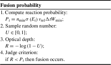
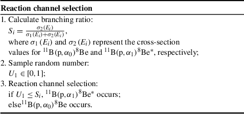




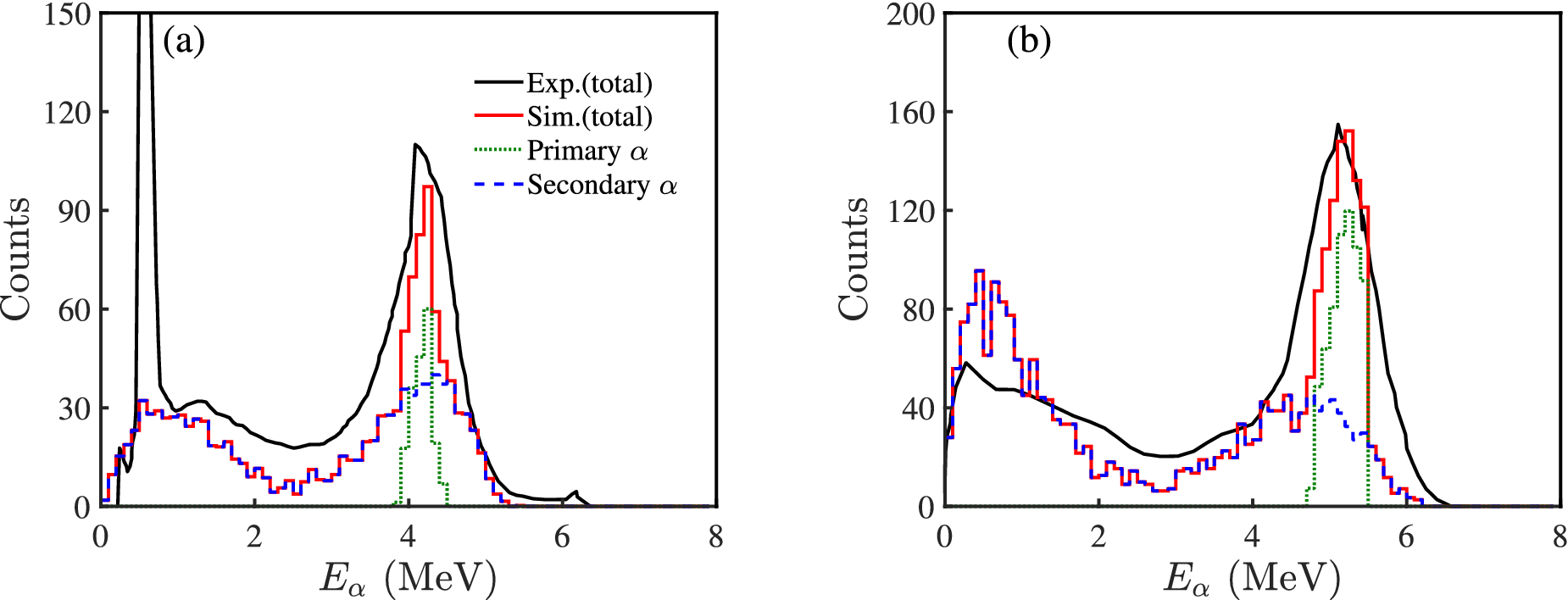


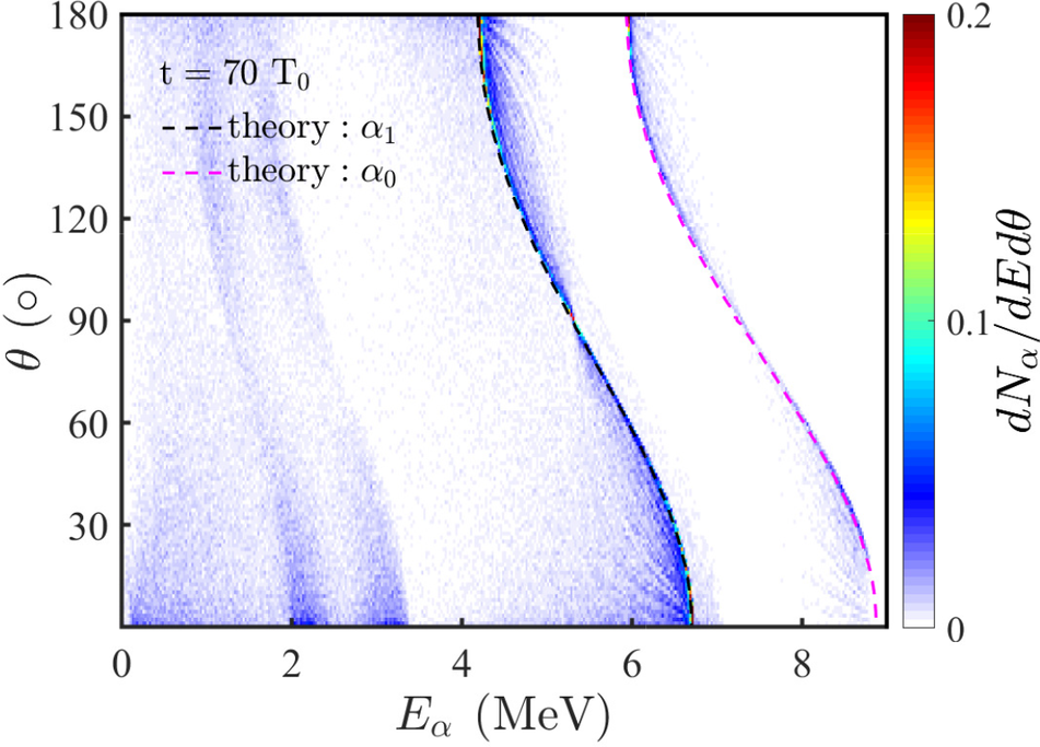


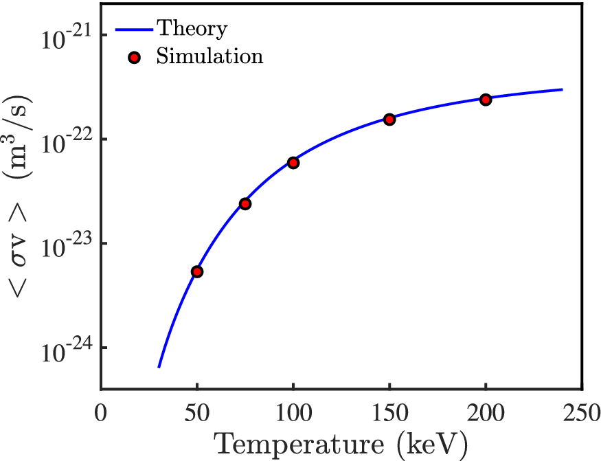


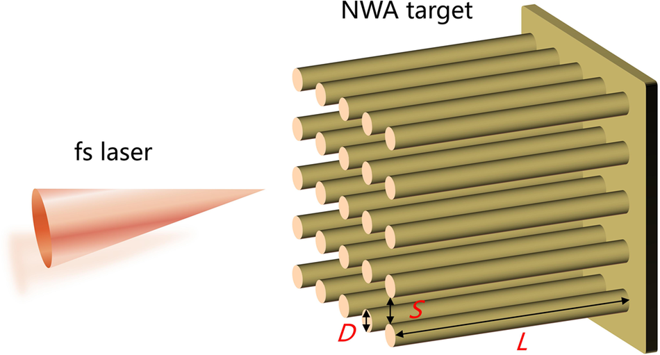


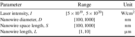
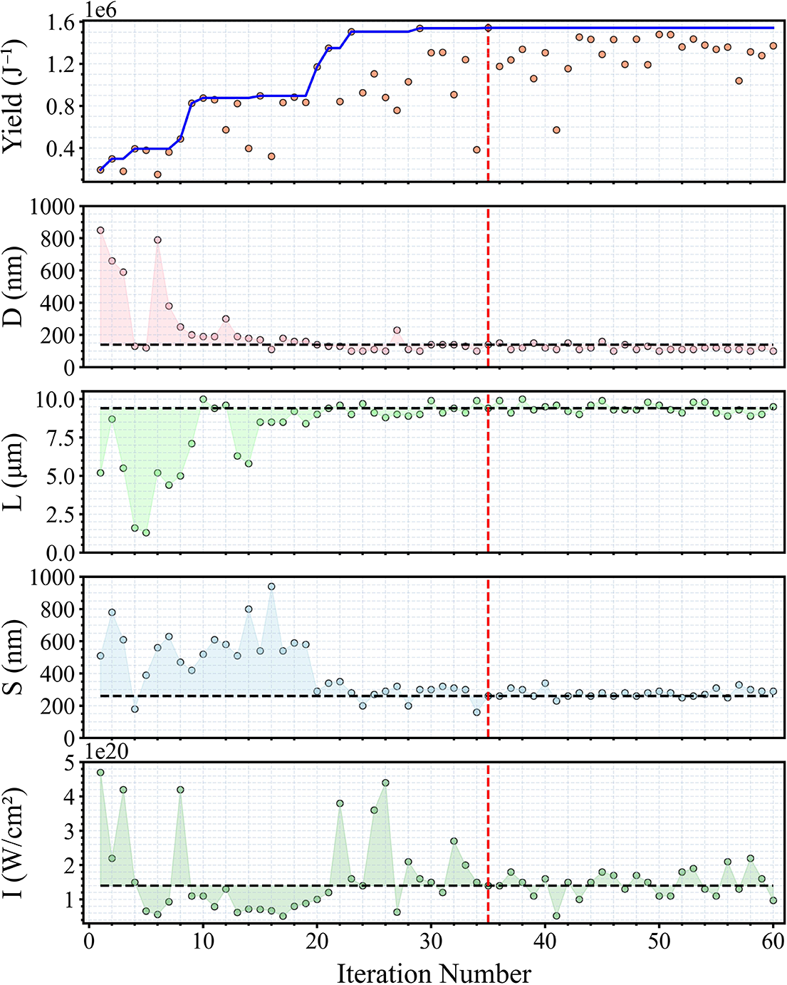


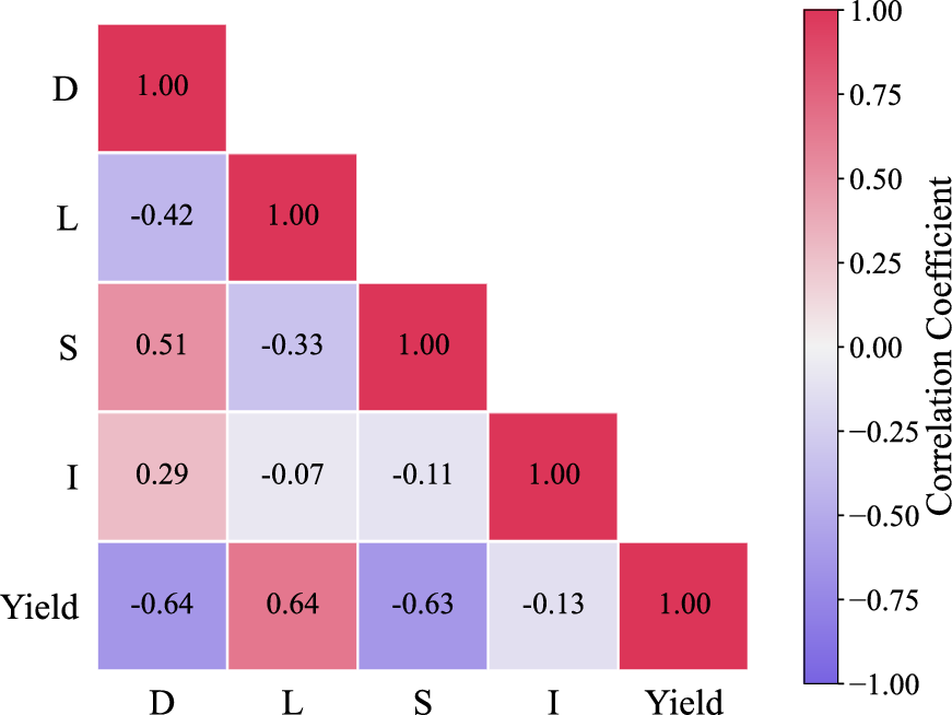

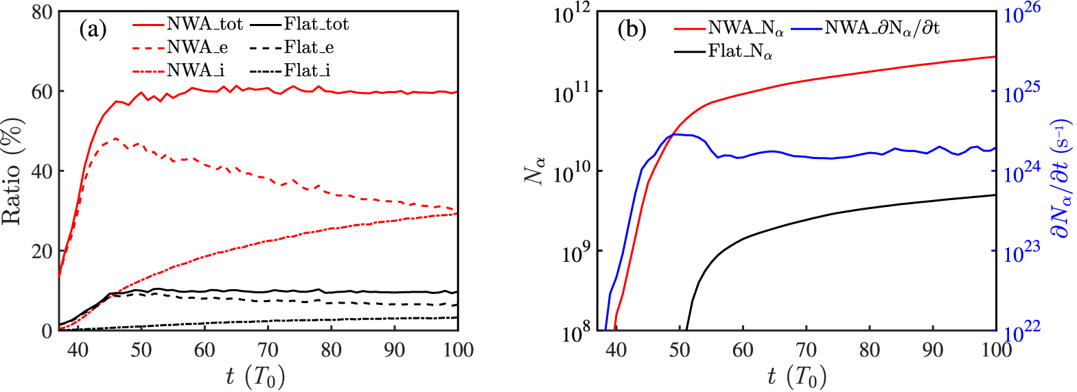


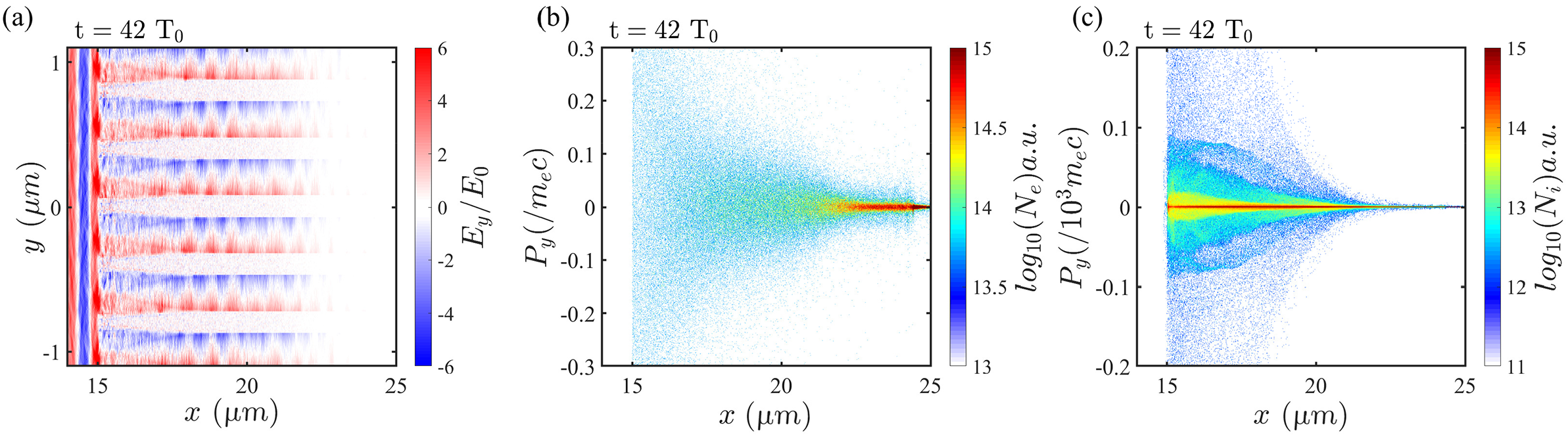


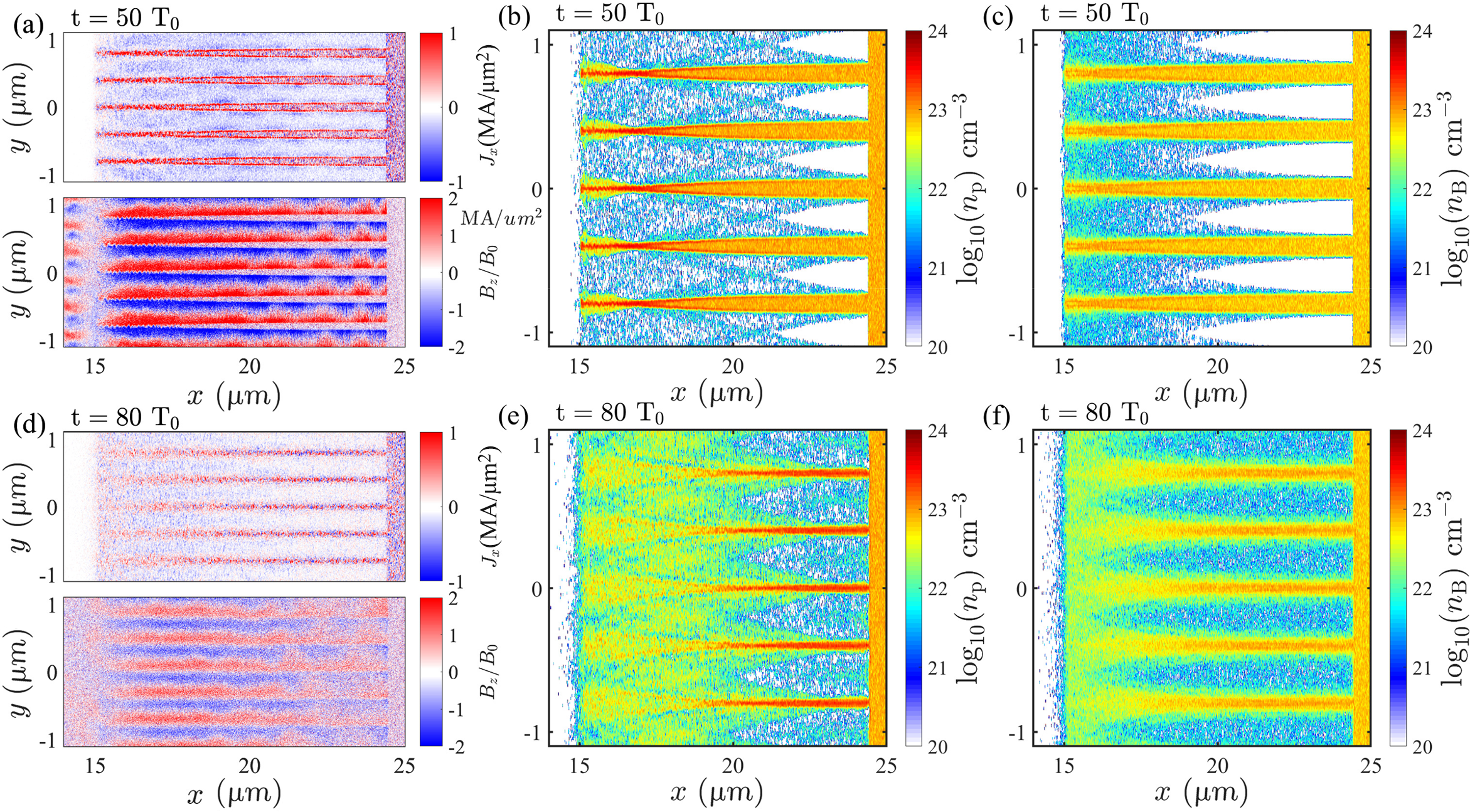


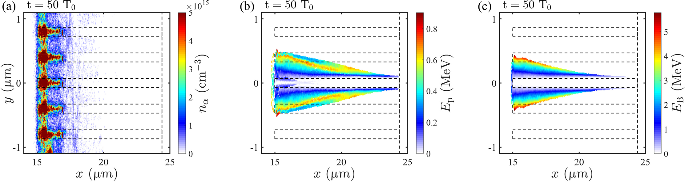


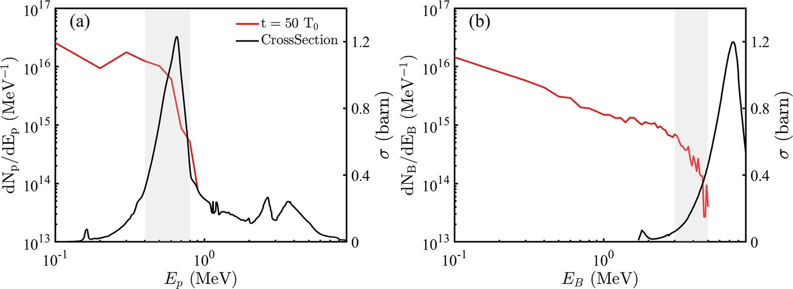


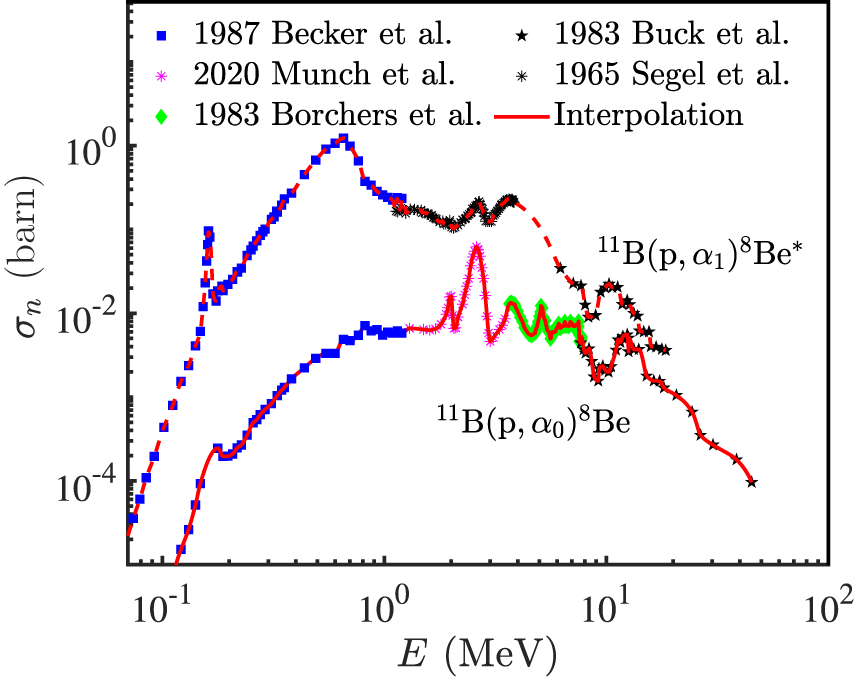


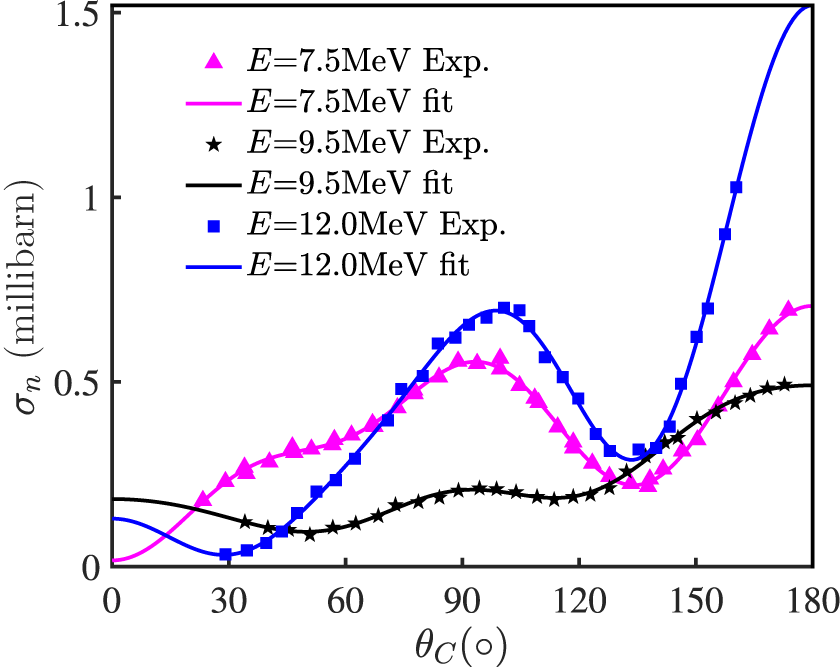


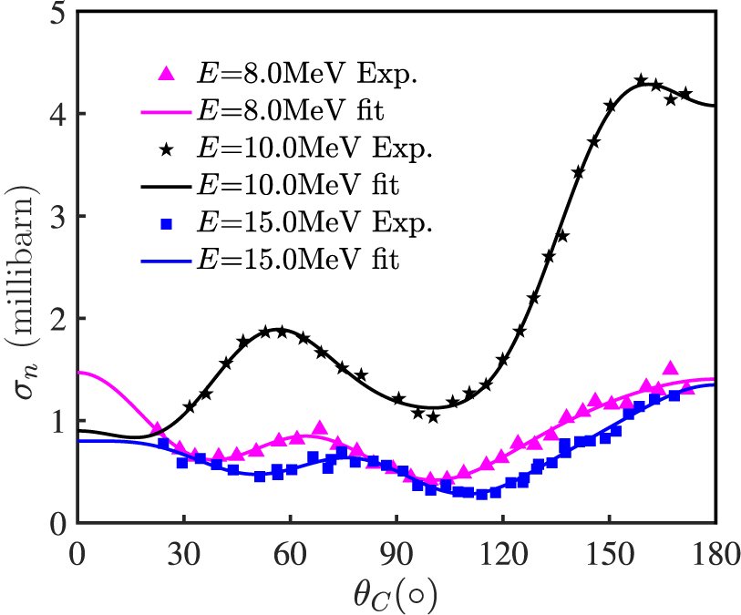


 Open access

