


1. Introduction
Characterizing the flow-induced reconfiguration of flexible structures has been the subject of intense research due to its relevance in various engineering, biological and environmental fields (Taylor Reference Taylor1952; Harder et al. Reference Harder, Speck, Hurd and Speck2004; Vollsinger et al. Reference Vollsinger, Mitchell, Byrne, Novak and Rudnicki2005; Stanford et al. Reference Stanford, Ifju, Albertani and Shyy2008; Vogel Reference Vogel2009). Flexible structures experience reduced drag,  $D$, compared with their rigid counterparts (Vogel Reference Vogel1984; Alben, Shelley & Zhang Reference Alben, Shelley and Zhang2002, Reference Alben, Shelley and Zhang2004; Gosselin, De Langre & Machado-Almeida Reference Gosselin, De Langre and Machado-Almeida2010; Luhar & Nepf Reference Luhar and Nepf2011; Leclercq & de Langre Reference Leclercq and de Langre2016; Hong et al. Reference Hong, Cheng, Houseago, Parsons, Best and Chamorro2022) due to deformation into streamlined shape, thus reducing the frontal area. This leads to changes in the typical drag's quadratic dependence with incoming flow velocity $U_0$ in rigid bodies at sufficiently high Reynolds number, resulting in $D \propto U_0^{2+V}$, where $V<0$ generally, is the so-called Vogel exponent. Evidence shows that the Vogel exponent depends on various parameters, including the geometry and material of the structure, buoyancy, skin friction and incoming flow mean shear. Alben et al. (Reference Alben, Shelley and Zhang2002, Reference Alben, Shelley and Zhang2004) showed that plates deform into quasiparabolic shapes when subjected to high flow velocity and found a Vogel exponent of $V \approx -0.67$. Gosselin et al. (Reference Gosselin, De Langre and Machado-Almeida2010) investigated the drag of two flexible object geometries subjected to a wide range of incoming velocity; they showed that the data can be collapsed to a single curve when normalized by a scale Cauchy number and the flexible object deformation also collapse to a quasiparabolic curve. Luhar & Nepf (Reference Luhar and Nepf2011) explored the role of blade stiffness and buoyancy on blade reconfiguration and proposed a model for drag and reconfiguration applicable to seagrass and microalgae in natural settings. Their model quantifies the degree of reconfiguration as a function of two dimensionless ratios: the Cauchy number, $Ca$, defined as drag to stiffness restoring force ratio; and the ratio between restoring force caused by buoyancy and stiffness-related restoring force.
Porous structures are paramount in various engineering systems and frequently encountered in nature; examples include coral groups, insect wings and seeds. Their ability to control aero- and hydrodynamic forces by modulating the degree of reconfiguration and the surrounding flow has been studied over the last decades (Tunnicliffe Reference Tunnicliffe1982; Santhanakrishnan et al. Reference Santhanakrishnan, Robinson, Jones, Low, Gadi, Hedrick and Miller2014; Cummins et al. Reference Cummins, Seale, Macente, Certini, Mastropaolo, Viola and Nakayama2018; Farisenkov et al. Reference Farisenkov, Lapina, Petrov and Polilov2020). Most studies have focused on rigid perforated bodies and showed that the drag coefficient decreases as the structure porosity increases (Guan, Zhang & Zhu Reference Guan, Zhang and Zhu2003; Bitog et al. Reference Bitog, Lee, Hwang, Shin, Hong, Seo, Mostafa and Pang2011; Basnet & Constantinescu Reference Basnet and Constantinescu2017). Dong et al. (Reference Dong, Luo, Qian and Wang2007, Reference Dong, Luo, Qian, Lu and Wang2010) also demonstrated that structure porosity affects the flow in the vicinity of a porous plate, which leads to a reduction of recirculation in the wake. Lee & Kim (Reference Lee and Kim1999) and Basnet & Constantinescu (Reference Basnet and Constantinescu2017) reported a lack of recirculation region immediately behind the porous plate if the porosity,  $\gamma$, is sufficiently high ( $\gamma \geq 35\,\%$). Recently, Singh & Narasimhamurthy (Reference Singh and Narasimhamurthy2022) performed direct numerical simulations on the wake of uniformly perforated plates and showed that the bleed-through perforation is the main reason for drag reduction. The onset of periodic Kármán vortex shedding was first noted by Castro (Reference Castro1971), who observed a critical porosity level for Reynolds numbers within the range of $2.5 \times 10^4 < Re < 9 \times 10^4$. Numerous studies have examined the relationship between drag coefficient and porosity dependence, with pressure loss being influenced by several parameters such as Reynolds number ( $Re$), porosity ratio ( $\gamma$) and Mach number ( $\mathit {Ma}$). Early models formulated by Betz (Reference Betz1920) proved helpful in a particular range of porosities but underestimated the drag coefficient at relatively low porosities. A model proposed by Koo & James (Reference Koo and James1973) scaled the wake velocity to match the boundary conditions but also underestimated drag at low porosity. Steiros & Hultmark (Reference Steiros and Hultmark2018) incorporated the impact of base suction, leading to improved drag predictions at low porosity.
Compared with their rigid counterpart, the interaction between flow and flexible porous structures has not been explored in detail. Guttag et al. (Reference Guttag, Karimi, Falcón and Reis2018) investigated the influence of base clamping on the static deformation of perforated plates. Recent work by Jin et al. (Reference Jin, Kim, Cheng, Barry and Chamorro2020) explored the mean drag, wake and reconfiguration of structure with various degrees of uniform porosity. They showed the possibility of a positive Vogel exponent for a sufficiently high porosity level, which was explained by a relatively high effective velocity near the structure. Despite the efforts to characterize the impact of porosity on flexible structures, these investigations solely considered uniform porosity over the plate. As a result, the effects of localized porosity and the influence of spatially distributed perforations on mean drag and deformation have been overlooked and remain mostly unexplored.
This study explores the impact of localized perforations on plate deformation and forces. We employ a combination of wind-tunnel experiments and direct numerical simulations to examine a wide range of parameters and gain valuable insights into the reconfiguration of plates. Section 2 provides detailed information about the experimental set-up, and § 3 discusses the main results. Finally, § 4 summarizes the key findings of the study.
2. Experimental set-up
The experiments were conducted in the Eiffel-type wind tunnel at the Talbot Laboratory of the University of Illinois. The wind tunnel is characterized by a test section of 6.10 m in length, 0.91 m in width and 0.45 m in height. The tunnel ceiling is adjustable to impose pressure gradients set to nearly zero along the test section.
We explored the reconfiguration of flexible plates with a single square perforation at different heights along their vertical axis. Square orifices, as canonical shapes, offer a comparatively simple method for characterization in relation to rectangular plates. Also, they complement research in various applications (e.g. Ibrahim et al. Reference Ibrahim, Al-Sammarraie, Al-Jethelah, Al-Doori, Salimpour and Tao2020). The plates had identical characteristics, namely, length  $L = 200$ mm, width $b = 50$ mm, thickness $c = 0.38$ mm, Young's modulus $E = 2.4$ GPa and density $\rho = 1180$ kg m $^{-3}$. The perforation had a side length of $a = b/3 = 16.7$ mm, resulting in a porosity ratio of $\gamma =a^2/(b L) \approx 0.028$. We tested the plates with single perforations at 11 positions along the vertical axis, with the perforation centred at $y/L=(2n-1)/24$ for $n=1,\ldots,11$. Hereafter, we use the nomenclature $P1$ to $P11$ to refer to the perforated plates, where $P1$ denotes the plate with the perforation at the base, and $P11$ refers to the plate with the perforation nearest to the tip. The solid plate without perforation is denoted by $P0$; see schematic in figure 1. Basic parameters, including the global and local coordinate systems, the local bending angle at perforation $\theta$ and an arclength $s$, are illustrated in figure 1(b). The global coordinate has the origin at the root of the plates, with $x$ and $y$ in the streamwise and wall-normal direction, whereas the local coordinate origin ( $x_0, y_0$) is set at the centre of the perforation and also points towards the streamwise and vertical directions, and $s = 0$ is at the root of the plate. We also examined selected rigid plates with perforations at three locations ( $P4$,
$P4$,  $P7$ and $P11$) and the base cases with rigid and flexible plates without perforations ( $P0$), which also served as a reference.
(a) Basic schematic of the experimental set-up (not scaled) illustrating the load cell, field of view (FOV), local horizontal-vertical coordinate  $(x_0, y_0)$ with origin at the centre of the perforation, (b) schematic of a plate illustrating arclength, $s$, and the local bending angle at perforated location, $\theta$, and (c) locations of the single perforations in the plate.

Although porosity could affect the plates’ structural characteristics, the equivalent bending stiffness  $EI_{eq}$ and mass per unit length $\rho _mA_{eq}$ only underwent minor changes. Following Luschi & Pieri (Reference Luschi and Pieri2014) and Barry & Tanbour (Reference Barry and Tanbour2018), these are given by
 \begin{equation} \left.\begin{array}{c} \rho_{m} A_{e q}=\dfrac{\rho_{m} b c(1-N(\gamma-2)) \gamma}{N+\gamma}, \\ E I_{e q}=E I \dfrac{(N+1) \gamma(N^{2}+2 N+\gamma^{2})}{(1-\gamma^{2}+\gamma^{3}) N^{3}+3 \gamma N^{2}+(3+2 \gamma-3 \gamma^{2}+\gamma^{3}) \gamma^{2} N+\gamma^{3}}. \end{array}\right\} \end{equation}
Here,  $I = bc^3/12$ is the second moment of area and $N=1$ for single perforation. From (2.1), the variation results in less than 3 % compared with the base case without perforation. Additionally, the aspect ratio of the plate, $L/b = 4$ and $L/c \gg 100$, minimizes the influence of the Poisson ratio (Jin et al. Reference Jin, Kim, Cheng, Barry and Chamorro2020).
The plates were affixed perpendicular to the top wall of the tunnel and oriented to face the incoming flow at the start of the tunnel test section, where the boundary layer was considered negligible. The gravitational and elastic restoring forces ratio,  $G = \Delta \rho g b c L^3 / (EI) \approx 3.76$ (Luhar & Nepf Reference Luhar and Nepf2011; Jin et al. Reference Jin, Kim, Cheng, Barry and Chamorro2020), show some gravitational effect on the plate deformation. We characterized the aerodynamic force and reconfiguration of each plate at 16 incoming velocities, $U_0$, ranging from 2 to 10 m s $^{-1}$ at intervals of $\Delta U_0 = 0.5$ m s $^{-1}$. This resulted in a Reynolds number range of $Re = U_0b/\nu \in [6.8, 33.8] \times 10^3$, where $\nu$ denotes the kinematic viscosity of air, and Cauchy numbers $Ca = \rho _f b L^3 U_0^2/ (EI) \in [3.8, 94.5]$, where $\rho _f = 1.293$ Kg m $^{-3}$ is the density of air. Note that, for the conditions under analysis, the flow can be described as incompressible, indicated by a Mach number $\mathit {Ma} < 0.03$.
A high-resolution ATI Gamma load cell was utilized to measure the aerodynamic forces accurately and torques at a sampling rate of 1 kHz for 90 s. Each force measurement was repeated thrice, resulting in a total measurement time of 270 s for each case. The minimum drag scenario had an uncertainty of approximately 3 % (Jin et al. Reference Jin, Kim, Cheng, Barry and Chamorro2020). To capture the deformation and vibration of the plates, a two-dimensional particle tracking velocimetry (PTV) technique was employed on 20 fiducial points equally distributed on the side of each acrylic plate. These fiducial points were illuminated by a halogen spotlight and captured using a 4 MP ( $2560 \times 1600$ pixel) Phantom M340 camera at a frequency of 100 Hz for duration of 30 s as shown in figure 1(a).
The flow field around the plates was characterized using particle image velocimetry (PIV). Two FOVs intersected at the centre of the plates were oriented perpendicularly to the wall and partially overlapped to produce a combined area of  $225\ \textrm {mm} \times 700\ \textrm {mm}$. The flow was seeded with 1 $\mathrm {\mu }$m olive oil droplets and illuminated by a 1 mm thick laser sheet created by a Quantel laser with a pulse energy of 250 mJ. A 4 MP CMOS camera captured 2400 image pairs of the FOVs at a frequency of 10 Hz. The images were analysed using TSI Insight 4G software with a recursive cross-correlation method and an interrogation window size of $24 \times 24$ pixel with 50 % overlap, resulting in a final vector grid spacing of $\Delta x = \Delta y = 1.68$ mm. The measurements were taken after the system reached a steady state, and a waiting period of at least 60 s was observed to minimize the initial transient effect.
3. Results
3.1. Baseline assessment: mean aerodynamic force of rigid plates
Figure 2 depicts the correlation between the flow velocity, the measured drag and the principal torque of the  $P0$ (solid), $P4$,
$P4$,  $P7$ and $P11$ rigid plates. The base plate without perforation follows the $U_0^2$ trend, illustrated as a dashed line. The plates with perforation display a lower level of drag and a marginal deviation from the quadratic pattern, as anticipated. The drag coefficient $C_d$ is defined by
 \begin{equation} C_d = F_x/ ( \tfrac{1}{2}\rho_f U_{0}^2 A ), \end{equation}
where  $A$ is the frontal area that accounts for the perforation. The rigid perforated plates exhibit a lower drag coefficient than the unperforated base plate, as illustrated in figure 2(b). This can be attributed to the jet that penetrates the wake of the cantilever plate. Notably, the $P1$ and $P4$ plates exhibit comparable, and the lowest drag, coefficients due to the jet's trajectory. The $P7$ and $P11$ plates display similar drag coefficients as highlighted in the inset of figure 2(b). A detailed discussion and basic modelling of the wake characteristics of the perforated plates is presented in § 3.3. The torque distribution in figure 2(c) reveals that the $P1$ plate had the largest torque, whereas the $P4$ and $P11$ plates had smaller values of $T_z$ compared with the $P7$ case, even though the $P1$ and $P4$ plates exhibited lower drag. Figure 2 demonstrates that the perforations affect the drag and alter the drag distribution over the plates.
(a) Mean drag,  $F_x$, (b) drag coefficient, $C_d$, and (c) main torque, $T_z$, of rigid perforated plates for various perforation locations: $P1$ (brown $\triangleright$); $P4$ (blue $\circ$); $P7$ (green $\diamond$); $P11$ (red $\triangle$); and incoming velocities. The solid $P0$ ( $\blacksquare$) plate is included as a reference, and the inset shows $C_d$ variation for various plates for a fixed $U_0$.

3.2. Mean aerodynamic force and reconfiguration of flexible plates
Here, we investigate the influence of various incoming velocities, namely the Cauchy number ( $Ca$) and Reynolds number ( $Re$) and relative perforation location on the reconfiguration and force coefficient of flexible plates. Although there was a general similarity in mean deformation across the plates under a given flow condition, discernible discrepancies in drag coefficients indicated that the position of the perforations has a critical impact on the plates’ dynamics.
Figure 3 depicts the measured drag, torque and drag coefficient  $C_d$ for several flexible plates, namely $P0$ (solid), $P1$,
$P1$,  $P4$,
$P4$,  $P7$ and $P11$, with the flexible base plate exhibiting a negative Vogel exponent of $V \approx -0.8$. As illustrated in figure 3(b), the perforated plates display lower $C_d$ values than the unperforated $P0$ base case. In fact, all perforated plates demonstrate a reduction in $C_d$, with this drag reduction being most prominent for plates with perforations at the root, i.e. the $P1$ plate. The $C_d$ monotonically increases as the perforation moves towards the tip of the plate, which results in the minimum $C_d$ reduction for the $P11$ case, as shown in the inset of figure 3(b). Notably, the difference in $C_d$ between the perforated $P11$ and the unperforated base case becomes insignificant at a higher incoming velocity $U_0 > 7$ m s $^{-1}$, indicating that the distribution of drag is not solely dependent on plate stiffness and porosity. The location of the perforation orifice also plays a crucial role in determining drag, even though the plate has the same porosity in its non-deformed state. Thus, it is crucial to consider an effective porosity for different perforation locations under bending.
Effect of perforation location on selected flexible plates:  $P1$ (brown $\triangleright$); $P4$ (blue $\circ$); $P7$ (green $\diamond$); $P11$ (red $\triangle$); the solid $P0$ ( $\blacksquare$) flexible plate is included as reference. (a) Drag force, (b) drag coefficient and (c) base torque, $T_z$. The inset in (b) shows $C_d$ variation for each plate at a fixed $U_0$, and the inset in (c) shows the torque difference between the base and perforated plates.

Figure 4 displays the drag coefficient obtained from both the experimental measurements and complementary direct numerical simulations (see the Appendix (A)), the latter including also the cases in which only the Cauchy number was varied while keeping the Reynolds number fixed at  $Re=10^3$. By combining the experimental and numerical results, we could examine a wider range of parameters and draw a conclusion on the significant role of the Cauchy number in controlling the reconfiguration and drag distribution of flexible plates, as previously reported in Luhar & Nepf (Reference Luhar and Nepf2011).
Drag coefficient,  $C_d$, from experiments (blue) and numerical simulations (red), as a function of the Cauchy number, $\mathit {Ca}$. Black symbols show additional numerical results at a fixed $Re=1000$. The inset shows $C_d$ as a function of $Re$.
$Re$.

The measured reconfiguration of three representative plates  $P0$ (unperforated), $P4$ and $P11$ at various incoming velocities is illustrated in figure 5. Additionally, figure 5(e,f) presents numerical results that enable direct comparison with experiments. Despite the small porosity resulting in similar deformation magnitudes for all plates, it is noteworthy that the plate with perforation at the base ( $P1$) exhibited the largest deformation across the $Ca$ range. In contrast, the plate with the perforation at the tip showed only minor changes compared with the base case at higher $U_0$ and a smaller deformation at lower incoming velocity. These differences in the mean plate deformation result from the combined effect of the local force and bending stiffness $EI_{local}$ distributions along the plate. The lower torque experienced by $P11$ plate (figure 3c) resulted in a smaller deformation at comparatively low flow velocity, whereas plate $P11$ showed a similar torque as the $P0$ base case at relatively high flow velocity due to a diminishing effect of porosity, leading to a similar deformation to the base case $P0$.
$P0$.
Measured reconfiguration of the  $P4$ (blue $\circ$) and $P11$ (red $\triangle$) plates, with the solid $P0$ ( $\square$) plate as a reference, under $U_0 =$ (a) 2, (b) 4, (c) 6 and (d) 8 m s $^{-1}$. Comparisons between measurements and simulations at $Ca \approx 4$ are shown for the (e) $P0$ and (f) $P11$ plates. Note that (e,f) are stretched in the abscissa to aid comparison.

3.3. Wake characteristics of flexible perforated plates
To investigate the impact of perforation location on drag and structural deformation, the flow field near the plates was analysed for specific incoming flow velocities,  $U_0 = 3$, 5 and 8 m s $^{-1}$, and perforation locations, plates P0 (solid), P4 and P11. The time-averaged streamwise velocity distribution is depicted in figure 6 for these cases. The presence of a jet-like structure emanating from the perforation is a crucial factor responsible for altering the wake of the plates. It should be noted that the low porosity of the perforations ( $\gamma \approx 0.028$) resulted in minimal changes to the backward flow region where $U(x,y) < 0$, in contrast to the significant backward flow region reduction observed in plates with high porosity (Jin et al. Reference Jin, Kim, Cheng, Barry and Chamorro2020).
Measured time-averaged streamwise velocity fields around the  $P0$ (solid), $P4$ and $P11$ flexible plates under $U_0=3$, 5 and 8 m s $^{-1}$. In (a–c), the white bar indicates the stitching edge of two PIV FOVs.

Basic characterization of a jet's structure involves an assessment of the spatial features of the jet centre, the time-averaged profile of the streamwise velocity along the centreline ( $U_c$), and the evolution of the time-averaged streamwise velocity's spanwise distribution at various downwind locations. These provide insight into the effects of the jet on the plate. The wake features are depicted in figure 7. The size of the jet is comparable to $2b_0$, which represents the width of the perforation, as illustrated in figure 7(d). On closer examination of the time-averaged streamwise velocity, as shown in figure 7(b), the jet centreline is curved, and the line of maximum velocity is denoted in black. The spanwise turbulence intensity is displayed in figure 7(c), where the red-dashed box denotes a low turbulence potential core that extends over a distance of $x_c$. A corresponding conceptual sketch is presented in figure 7(d).
(a) Characteristics of the measured jet through the perforation in the  $P4$ plate under $U_0 = 3$ m s $^{-1}$. (b) Mean streamwise velocity, $U/U_0$. The black line indicates the jet centre. (c) Streamwise turbulence intensity, $\sigma _u/U_0$. The red-dashed box shows the potential core. (d) Conceptual diagram of the jet.

Figure 8 illustrates the distributions of normalized velocity for the jet centre,  $U_c/U_0$, for the $P4$ and $P11$ plates at various incoming flow velocities. The velocity profiles exhibit typical characteristics of a turbulent jet centreline, with a relatively constant velocity within the potential core and a linear decrease downstream, as described in Pope (Reference Pope2000). In contrast to the constant gradient for water jet velocities (Giralt, Chia & Trass Reference Giralt, Chia and Trass1977; Rajaratnam, Zhu & Rai Reference Rajaratnam, Zhu and Rai2010; Shademan, Balachandar & Barron Reference Shademan, Balachandar and Barron2013), current measurements show that the slope varies between cases with $U_0$ and perforation location. At low $U_0$, a lower normalized velocity is evident within the potential core, while the centreline profile decays faster outside the potential core at higher $U_0$, with $U_c/U_0$ approaches zero at a shorter distance $(x-x_c)/b_0$ from the potential core, leading to a shorter bulk jet. Moreover, a comparison of jet profiles for different perforation locations at the same $U_0$ in figure 8(a,b) suggests a shorter jet length for the perforation located near the tip, i.e. the $P11$ plate.
Measured jet centre velocity,  $U_c/U_0$, for the (a) $P4$, and (b) $P11$ flexible plates.

A possible way to characterize the influence of incoming velocity and perforation location on the distribution of the jet centreline velocity  $U_c$ could be through a single parameter. Figure 9 presents the normalized $U_c$ by the corrected incoming velocity $U_0 \cos {\theta }$ and corrected perforation half-width $b_0 \cos {\theta }$, where these quantities are determined as the $U_0$ component perpendicular to the perforation and the projected $b_0$ in the streamwise direction. This first attempt results in a similar normalized jet length $(x-x_c)/b_0\cos {\theta }$ for all cases; however, it further deviates the normalized exit velocity at $(x-x_c) = 0$.
Measured jet centre velocity normalized by corrected incoming velocity,  $U_c/(U_0 \cos {\theta })$ with normalized distance by effective perforation half-width, $(x-x_c)/(b_0 \cos {\theta })$, for the (a) $P4$, and (b) $P11$ plates.

Inspection of scaling with velocity  $U_0$ appears inappropriate for representing $U_c$ profiles. This is because the flow near the structures is significantly affected by the windward side of the body (Hemmati, Wood & Martinuzzi Reference Hemmati, Wood and Martinuzzi2016; Liu et al. Reference Liu, Hamed, Jin and Chamorro2017; Jin et al. Reference Jin, Kim, Cheng, Barry and Chamorro2020), making it crucial to consider the effective velocity $U_e$ at the perforation. Here, $U_e$ is defined as the velocity experienced in the proximity of the perforation at a location $d/b_0 = 4$ upwind of the front surface of the plate (Jin et al. Reference Jin, Kim, Cheng, Barry and Chamorro2020). To assess the influence of the effective velocity, figure 10(a) illustrates the distribution of $U_e$ for the $P4$ plate at various $U_0$. As $U_0$ increases, the $U_e/U_0$ ratio also increases, mainly due to the higher plate deformation, as depicted in figure 5. Furthermore, the plate near the tip is more streamlined than its root, resulting in a higher $U_e$. The inset of figure 10(a) displays the spatially averaged $U_e$ along the plate arclength, $s$, at various upwind locations $d/b_0 = 3.5 - 4.5$, revealing a similar distribution. The use of the corrected effective velocity, $U_e \cos {\theta }$, and corrected perforation half-width, $b_0 \cos {\theta }$, to normalize $U_c$ in figure 9 allows the profiles at different $U_0$ and perforation locations to collapse onto an approximately linear trend with a slope of $\beta = -1/4$ for $x > x_c$. This suggests that the distribution of $U_c$ is a function of the effective local velocity and local bending angle and can be expressed as $U_c = f(U_e,\theta ) \approx -0.25(x-x_c)U_e/b_0 + 2.05 (U_e \cos {\theta })$.
(a) Measured effective velocity,  $U_e$, at $d/b_0 = 4$ from the $P4$ plate for $U_0 = 3$, 5 and 8 m s $^{-1}$; the dashed line in the schematic illustrates the location used for the effective velocity, and the inset shows spatially averaged $U_e$ at $d/b_0 = -3.5$, $-$4 and $-$4.5. (b) Renormalized centre jet centrevelocity, $U_c/(U_e\cos \theta )$, with normalized distance by effective perforation half-width $(x-x_c)/(b_0 \cos {\theta })$.

Transverse jet profiles are shown in figure 11(a,c), with the  $P4$ plate at $U_0 = 8$ m s $^{-1}$ and the $P11$ plate at $U_0 = 3$ m s $^{-1}$ serving as examples. The profiles display dissimilar diffusion rates for the upper, $y - y_0 > 0$, and lower, $y - y_0 < 0$, sections of the jets, with slower diffusion at $(y-y_0)/b_0 < 0$ for the $P4$ plate subjected to 8 m s $^{-1}$ flow, due to the lower turbulence levels, similar to those presented in figure 7(c). Despite these differences, both jet segments exhibit self-similar characteristics as they progress downwind, as shown in figure 11(b,d), conforming to the standard Gaussian distribution
 \begin{equation} \frac{u}{u_{max }}=\exp \left(-\frac{y^2}{2 \sigma^2}\right), \end{equation}
where  $\sigma$ is the standard deviation. Additionally, the condition of dynamic similarity is satisfied as indicated by Albertson et al. (Reference Albertson, Dai, Jensen and Rouse1950), leading to a constant diffusion angle such that
 \begin{equation} (x-x_0)/\sigma = C. \end{equation}
Selected transverse profiles of time-averaged streamwise velocity of the jets through perforations from numerical simulations: (a)  $P4$ plate, $U_0 = 8$ m s $^{-1}$; (b) normalized profiles; (c) $P11$ plate, $U_0 = 3$ m s $^{-1}$; (d) normalized profiles; (e) Schematics of a Gaussian distribution. Here $\sigma$ denotes the distance where $U/U_{max}=0.605$. Insets show the $\sigma$ with distance.

The inset of figure 11(b,d) illustrates the  $\sigma$ evolution at various downwind distances and yields the diffusion rate $C$, which indicates a higher value for the upper side jet that is approximately twice the value for the bottom side counterpart. This result provides evidence that the local shear (or turbulence intensity) outside of the potential core influences $C$, such that $C = f(\sigma _u)$, where $f$ is an empirical function fitted to the current experimental data. Given the information about $U_c$ and $C$, and assuming a linear decay of potential core width from $w = 2 b_0$ at $x = x_0$ to zero at $x = x_0 + x_c$, the predicted velocity profiles of the empirical model are shown in figure 12 as a red-dashed line for various downwind locations. The semiempirical modelled profiles agree well with the experimental data represented by the blue circles.
Comparison between experimental (blue  $\circ$) and modelled (red – –) transverse jet profiles from the perforations at various downwind locations for the plate $P4$ under $U_0 = 3$ m s $^{-1}$. The grey area denotes the potential core region.

Further analysis through numerical simulations allowed for the investigation of the jet centreline trajectory, jet centreline profiles and the effective velocity distribution at a fixed Reynolds number of  $Re = 1000$ (which is one order of magnitude lower than the experimental cases), allowing us to separate the Reynolds and Cauchy number influences. By adjusting the blade's stiffness, we simulated three Cauchy numbers of $Ca = 0.1$, 7 and 75, thus spanning a wider range for this parameter.
Figure 13 displays a similar streamwise velocity pattern observed in the simulations if compared with the experimental results (shown in figure 6). The jet centreline profiles’ collapse in figure 14 confirms that  $Ca$ is the dominant parameter, while the jet centreline velocity demonstrates independence from the Reynolds number for $Re \in [0.1, 3.4] \times 10^4$. Moreover, the centreline trajectory is primarily a function of $Ca$ and perforation location as it is affected by the wake recirculation zones, as shown in figure 15(a), which depicts streamlines in the wake of the $Ca = 0.1$ base plate without perforation. The jet centreline trajectory also allows us to define an exit angle of the jet, $\alpha$, as shown in figure 15(b). The subsequent section will provide additional insight into how this exit angle $\alpha$ affects the local jet thrust, consequently impacting the plate's bulk drag.
Time-averaged streamwise velocity field at  $z=0$ around the (a–c) $P4$ and (d–f) $P11$ plates at $Ca = 0.1$, 7 and 75 for $Re=1000$ from numerical simulations.

Normalized jet centre velocity,  $U_c/U_e \cos {\theta }$, with normalized downwind distance, $(x_0-x_c)/b_0 \cos {\theta }$, for various $Ca$ and $Re$ using numerical simulations and experiments.

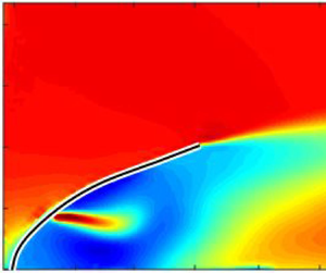
(a) Time-averaged streamwise velocity distribution around the  $P0$ (solid) plate at $Ca = 0.1$ from simulation; white curves denote streamlines highlighting the recirculation region. Jet centreline trajectories for the (b) $P4$ and (c) $P11$ plates for various $Ca$.
$Ca$.

3.4. A first-order formulation for drag in perforated plates
As a basic estimation, figure 6 demonstrates that the total drag on the plate can be partitioned into two distinct constituents: namely, the drag acting solely on the plate and the force change by the perforation as
 \begin{equation} C_d \approx C_{d,P0} - C_{T,jet}. \end{equation}
The presence of the jet induces modifications in the local thrust, which can be computed by carrying out a momentum integral over a control volume that encloses the jet. Then, the force coefficient  $C_F$ can be estimated based on this value as
 \begin{equation} C_F=\frac{2b}{A} \int_{{-}H}^{{+}H} \frac{U(y)}{U_{\infty}}\left(\frac{U(y)}{U_{\infty}}-1\right) \mathrm{d}\kern0.05em y. \end{equation}
Typically, the selection of  $U(y)$ and $H$ in the momentum integral is based on the premise that they are sufficiently far away from the perforated plate to render the contribution of pressure and velocity fluctuations negligible in the integrand (Ramamurti & Sandberg Reference Ramamurti and Sandberg2001; Bohl & Koochesfahani Reference Bohl and Koochesfahani2009). However, due to the proximity of the perforations to the shear layer and the wake generated by the plate, disentangling the impact of pressure and velocity fluctuations between the jet and wake becomes challenging for the far downstream $U(y)$ profile. Therefore, $U(y)$ profiles in the vicinity of the perforation (i.e. $x_0 = 0^+$) are selected for the momentum integral, where the contribution of the jet passing through the perforation dominates, and $H = b_0$ is chosen for integration. This selection yields a uniform velocity profile with a width of $2b_0$, exhibiting minimal velocity fluctuations within the potential core, as depicted in figures 7(c) and 12. The estimation of thrust is expressed as
 \begin{equation} \left.\begin{array}{c} T_{jet,model} \propto \dot{m} U_{c, x=0} \cos \alpha \propto \rho A U_e^2 \cos^2 \theta \cos \alpha =\gamma_{3D} \rho A U_e^2 \cos^2 \theta \cos \alpha,\\ C_{T_{jet,model}} = T_{jet, model}/(\frac{1}{2}\rho_fU_0^2A), C_{T_{jet,exp}} \approx C_{d_{P0}} - C_{d_{P_i}}, \end{array}\right\} \end{equation}
where  $\alpha$ is the exit angle of the jet obtained from the jet centreline trajectory in figure 15(b,c). The coefficient $\gamma _{3D}$ takes into consideration geometry-dependent factors that account for three-dimensional wake effects. In the case of rigid plates, the ratio $U_e/U_0$ remains constant across a broad range of $U_0$, and $\cos \theta = 1$. The difference in force between the plates is directly proportional to $\cos \alpha$. As depicted in figure 16(a), the measured and estimated $C_d$ values are compared using (3.6). The $P4$ case exhibits a nearly straight centreline, resulting in the highest local thrust and, therefore, the lowest total drag. An upward tilting trajectory results in larger $\alpha$ values for the $P11$ plate, resulting in a smaller $C_d$.
(a) Comparison of measured and modelled  $C_d$ for rigid plates under $U_0 = 3$ m s $^{-1}$, (b) measured $Ue/U_0$ for the $P4$ and $P11$ flexible plates, (c) measured local bending angle, $\theta$, (d) measured and estimated local jet thrust coefficient, $C_T$, for the $P4$ and $P11$ flexible plates. The dashed line represents the estimation using a default $\gamma _{3D} = 1$.

The experimental trends of  $U_e/U_0$ and $\theta$ obtained from the experiments are employed in (3.6) to estimate the total drag of the flexible plates, as illustrated in figure 16(b,c). Figure 16(d) compares the modelled local jet thrust coefficient $C_T$ and the measured values. The experimental $C_T$ are computed by subtracting the drag coefficient of the perforated plates $C_{d,Pi}$ from the base plate drag coefficient $C_{d,P0}$ provided in (3.6). The predicted $C_T$ obtained using a default $\gamma _{3D} = 1$ yields a higher value than the experimental measurement of $C_T$. The observed deviation in thrust within the simple model can be attributed to two primary factors. First, three-dimensional effects play a varying role. Second, as the $Re$ increases, the accuracy of the basic jet thrust estimation diminishes. This discrepancy arises from the omission of pressure and velocity fluctuation terms in the momentum balance, resulting in an overestimation of the jet thrust. Although the model overlooks the downwind momentum adjustment, it captures the general trend of how the perforations affect the drag of the flexible plates, taking into account the various perforation locations and $U_0$. The value of $C_T$ estimated through (3.6) indicates the effective porosity of the flexible structures with square perforations at a particular $Ca$ since both the plate reconfiguration and $U_e$ are functions of the Cauchy number. The impact of the perforation reduces with the growth of $U_0$ ( $Ca$), owing to an increase in $\theta$. The location of the perforation dictates the reduction rate of such effective porosity, with perforations positioned closer to the tip exhibiting a substantially higher reduction rate in $C_T$. The $C_T$ values for $P4$ and $P11$ are nearly identical at $U_0 \approx 3$ m s $^{-1}$, but $P11$ experiences a much sharper decay for $U_0 \leq 5$ m s $^{-1}$. Furthermore, both $P4$ and $P11$ cases exhibit a slower reduction rate of $C_T$ for $U_0 > 5$ m s $^{-1}$ as $\theta$ increases marginally after a sufficient amount of bending experienced by the flexible plates.
4. Remarks and conclusions
Our study provides a comprehensive analysis of the influence of localized perforations on the dynamics of flexible plates subjected to uniform flow conditions with negligible turbulence. By conducting wind-tunnel experiments and direct numerical simulations, we investigated a wide range of parameters, including the perforation location, Cauchy and Reynolds numbers. We systematically observed a trend in the plate reconfiguration, the wake of the perforated plates and the corresponding aerodynamic force. The wake of perforated plates is characterized by a jet-like structure passing through the perforation orifice, and we modelled this jet by scaling its centreline velocity with a corrected effective local velocity,  $U_e \cos {\theta }$, and its length scale with the corrected half-width of perforation, $b_0 \cos {\theta }$.
Additionally, we propose a first-order formulation for estimating the bulk drag of perforated plates as the drag of the unperforated base plate minus the thrust generated by the jet passing through the perforation orifice. This jet thrust decreases as  $U_0$ increases due to an increase in local bending angle, $\theta$, illustrating how effective porosity decreases as $Ca$ increases. Our results may have implications for the aeroelastic characterization of flexible structures with non-homogeneous, localized porosity, a relatively underexplored topic with potential relevance to many engineering applications. Our study also establishes a fundamental basis for further research focusing on other geometrical features, such as different perforation shapes or sizes and flow regimes. Such studies would enhance our understanding of the complex interaction between flow and structures with low porosity and could facilitate the design of flexible structures with improved aerodynamic performance.
Acknowledgements
S.O. and M.E.R. acknowledge F. Viola for sharing the simulation code and the computational resources on the Saion cluster provided by the Scientific Computing section of the Research Support Division at OIST. The Okinawa Institute of Science and Technology Graduate University (OIST) supported the two authors with subsidy funding from the Cabinet Office, Government of Japan.
Funding
S.O. is also supported by grant FJC2021-047652-I funded by MCIN/AEI/10.13039/501100011033 and European Union NextGenerationEU/PRTR.
Declaration of interests
The authors report no conflict of interest.
Appendix A. Numerical study
A computational investigation was carried out to complement the experimental range and to explore the three-dimensional flow field, enabling the examination of lower Reynolds numbers (i.e.  $Re \lesssim 5 \times 10^3$) and the separation of the effects of the primary dimensionless governing parameters, specifically Reynolds and Cauchy numbers.
We employed the in-house flow–structure interaction solver AFiD (Viola et al. Reference Viola, Spandan, Meschini, Romero, Fatica, de Tullio and Verzicco2022). The code is based on the fractional-step method that solves the incompressible Navier–Stokes equations, (second-order) centred finite-difference for spatial discretization and (second-order) Adams–Bashforth and Crank–Nicolson scheme for temporal discretization of the nonlinear and diffusive terms, respectively (Viola, Meschini & Verzicco Reference Viola, Meschini and Verzicco2020; Viola et al. Reference Viola, Spandan, Meschini, Romero, Fatica, de Tullio and Verzicco2022). An immersed boundary method, based on a direct forcing and moving least-squares interpolation (de Tullio & Pascazio Reference de Tullio and Pascazio2016), is used to model the flow–structure interaction and indirectly impose the no-slip boundary condition between the fluid and the solid surface. The structural dynamics of the elastic structures is solved using a spring-network model for thin membranes (Viola et al. Reference Viola, Meschini and Verzicco2020). The computational framework has been validated in a variety of flow–structure interaction test cases (de Tullio & Pascazio Reference de Tullio and Pascazio2016; Olivieri et al. Reference Olivieri, Viola, Mazzino and Rosti2021).
The chosen computational domain is a box of size  $L_x / b = 16$, $L_y / b = 8$ and $L_z / b = 6$ along the streamwise, wall-normal (vertical) and spanwise directions, with the origin of the reference frame coinciding with the midpoint of plate root. The inlet of the domain lies at $x/b = -2$, at which a Dirichlet condition imposing uniform velocity is applied, while a convective boundary condition is used at the outlet ( $x/b = 14$). The no-slip condition applies at the bottom ( $y=0$) and top ( $y=L_y$) boundary, whereas periodic conditions apply over the lateral boundaries $z = \pm L_z / 2$. The domain is discretized with a uniform grid spacing $\Delta / b \approx 0.027$. Negligible differences in the main quantities of interest (e.g. plate deformation, aerodynamic forces and characteristic frequencies of motion) were found when increasing the domain size and numerical resolution.
The simulations considered the same plate geometries as the experiments and focused on cases where the perforations were located at positions  $P4$ or $P11$ and the unperforated case ( $P0$). To facilitate direct comparison between the experimental and numerical results, the simulations first addressed the lowest incoming flow velocity tested in the wind tunnel, which was $U_0 = 2$ m s $^{-1}$. Subsequently, two additional cases were simulated at lower Reynolds numbers, with plate relative flexibility (i.e. Cauchy number) varied in proportion to the change in wind velocity. Finally, a series of simulations were conducted at a fixed Reynolds number of $10^3$, with the Cauchy number varied over nearly four orders of magnitude, ranging from approximately $10^{-1}$ to $3\times 10^2$. A representative snapshot from one of the performed runs is given in figure 17.
Numerical simulation snapshot of case  $P11$ at $Re = 1000$ and $\mathit {Ca} \approx 7$, showing (a) a wall-normal plane at $z=0$ and (b) two horizontal planes colouredby instantaneous streamwise velocity – one passing through the perforation and the other slightly above the plate root. The grey horizontal plane indicates the solid boundary.


 Open access