

1. Introduction
Presently occurring changes in the Earth's climate and the cryosphere cause changes in sea level, and the societal relevance of these natural processes motivates a prediction of sea-level rise in the next decades and centuries (Reference ZwallyWarrick and Oerlemans, 1990; Reference PachauriPachauri and Reisinger, 2007; Reference SolomonSolomon and others, 2007). The multitude of physical processes contributing to sea-level change necessitates in-depth studies that are now summarized in the 2013/14 Intergovernmental Panel on Climate Change (IPCC) Assessment Report 5 (Reference Vaughan and StockerVaughan and others, 2013), and new observations as well as recent improvements in physical models may facilitate a more accurate assessment. Towards this goal, our study fills a specific gap that has not received much previous attention.
Mass transfer from ice sheet to ocean occurs largely through outlet glaciers via calving and meltwater processes. Outlet glaciers typically have a higher velocity than the neighboring inland ice, and often the acceleration is caused by the existence of a morphological trough or trough system in the bedrock. In addition, the fast-moving outlet glaciers of the Greenland and Antarctic ice sheets tend to react most rapidly to warming, as spatial acceleration tends to increase with increased sliding and in many cases through enhanced ice–ocean interaction at the grounding line of fjord glaciers, though there are exceptions (Reference Steffen and SteffenSteffen and Box, 2001; Reference Johnson, Prescott and HughesJohnson and others, 2004; Reference Podlech and PodlechPodlech and Weidick, 2004; Reference TimmermannThomas and others, 2004; Reference Rignot and RignotRignot and Kanagaratnam, 2006; Reference Hall, Williams, Luthcke and DigirolamoHall and others, 2008; Reference Mayer and HerzfeldMayer and Herzfeld, 2008; Reference Bevan, Murray, Luckman, Hanna and HannaBevan and others, 2012; Reference Rignot, Fenty, Menemenlis and MenemenlisRignot and others, 2012; Reference Sutherland and SutherlandSutherland and Straneo, 2012).
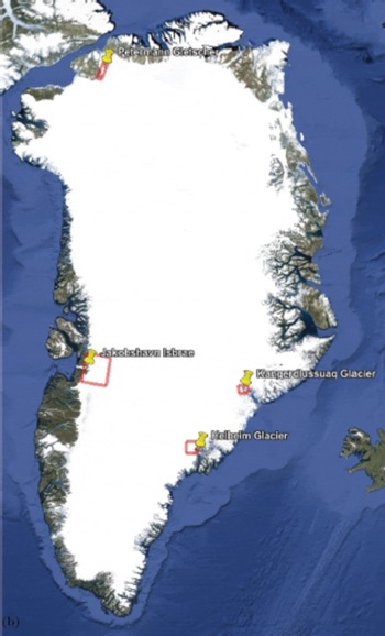
Dynamic ice-sheet models are used to estimate the contribution of mass loss from the Greenland and Antarctic ice sheets (Reference Gillet-ChauletGillet-Chaulet and others, 2012; Reference BindschadlerBindschadler and others, 2013; Reference GoelzerGoelzer and others, 2013; Reference NowickiNowicki and others, 2013a,Reference Nowickib). However, most models of the Greenland ice sheet do not include major subglacial troughs nor address the processes unique to them. If ice-sheet models are to correctly assess the maximum sea-level rise potential, then the accelerating effect of troughs in bed topography needs to be included, which requires inclusion of sub-scale troughs and trough systems at proper generalization (Reference Herzfeld, Fastook, Greve, McDonald, Wallin and ChenHerzfeld and others, 2012). A problem lies in the fact that subglacial troughs of most outlet glaciers are features of a scale that is close to the resolution of most ice-sheet models. Major outlet glacier troughs, such as that of Jakobshavn Isbræ, were generally missing in the bed topography used in many modeling studies (Reference Bamber, Layberry and GogineniBamber and others, 2001), and bed topography was not a concern of the modeling community until recently. A second problem in properly representing troughs in bed topography grids is caused by the measurement process. Typically, ice-penetrating radar is used to collect ice-thickness data. In narrow canyons the radar signal may be reflected from the sides of the canyons rather than the bottom, which may result in missing measurements of the largest depths or thicknesses. We have pioneered a mathematical approach that allows integration of subglacial troughs and trough systems in a topographically and morphologically correct generalization to any modeling scale, and applied this to recently collected radar data of Jakobshavn Isbræ (Reference Herzfeld, Wallin, Leuschen and PlummerHerzfeld and others, 2011a). This paper describes the mathematical algorithm and a generalization that allows the integration of subglacial troughs as well as trough systems, which may consist of several branches, into any spatial elevation model of subglacial topography. The algorithm is then applied to recently collected radar data of major outlet glacier regions, the Jakobshavn Isbræ, Helheim, Kangerdlussuaq and Petermann glacier regions (Fig. 1). The specific resultant JakHelKanPet digital elevation model (DEM) of Greenland subglacial topography has already been applied in several modeling studies (Reference Herzfeld, Fastook, Greve, McDonald, Wallin and ChenHerzfeld and others, 2012; Reference Greve and HerzfeldGreve and Herzfeld, 2013) and is used by the SeaRISE (Sea-level Response to Ice Sheet Evolution) community (e.g. Reference BindschadlerBindschadler and others, 2013; Reference NowickiNowicki and others, 2013a,Reference Nowickib), hence this paper serves as a description of this dataset for those who use it. The algorithm is more generally applicable at any grid resolution and in connection with any general Greenland bed topography. Recently released Greenland and Antarctic bed topography models include those of Reference Le Brocq, Payne and VieliLe Brocq and others (2010), Reference TimmermannTimmermann and others (2010), Reference BamberBamber and others (2013) and Reference FretwellFretwell and others (2013); however, the trough problem has not been treated there.
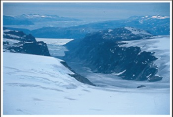
Location of trough-system areas in Greenland. Size and location of subarea outlines match coordinates given in Section 6. Background from Google Earth (http://earth.google.com).
2. Example of an Outlet Glacier: Subglacial Topography and Surface Roughness Indicative of Spatial Acceleration
This section serves to illustrate the relationship between bed topography, acceleration and surface features (e.g. crevasses) for the example of an outlet glacier. The main southern branch of Jakobshavn Isbræ, the fastest-moving glacier in Greenland, follows a subglacial trough. Figure 2 shows that the fast ice movement of Jakobshavn Isbræ south ice stream, which is indicated by heavy crevassing that extends >80 km into the ice sheet, is caused by the existence of the trough. The crevassing is evident in a color composite of the high-resolution (15m pixel) bands 1, 2, 3 of Advanced Spaceborne Thermal Emission and Reflection Radiometer (ASTER) data from the Terra satellite. Subglacial topography is contoured from a preliminary data-aggregation grid derived from CReSIS MCoRDS data (see Section 3). In contrast, Jakobshavn Isbræ north ice stream, which is also heavily crevassed and joins the south ice stream close to the 2003 calving front, does not follow a subglacial trough but lies at the end of a shallow depression.
Jakobshavn Isbræ (Ilulissat Ice Stream) surface structure, crevassing, spatial surface roughness and subglacial topography. Terra ASTER (Advanced Spaceborne Thermal Emission and Reflection Radiometer) data (band 1, 2, 3 color composite, background image) collected May 2003 show calving front and crevassing indicative of fast-moving ice and the shear margins. Subglacial topography contoured from CReSIS MCoRDS data (right color bar; see Section 3). Jakobshavn Isbræ south ice stream follows a deep subglacial trough. Universal Transverse Mercator (UTM) coordinates. Surface roughness derived from ICESat GLAS laser 3I data; pond parameter, derived from residual vario function of L3I along-track elevations, is highest over the shear margins of the south and north ice streams (left color bar indicates pondres value (m2) as shown along the GLAS tracks; red line visualizes roughness value pondres as distance from track).
Spatial surface roughness properties calculated from Geo-science Laser Altimeter System (GLAS) data collected during NASA's Ice, Cloud and land Elevation Satellite (ICESat) mission (Reference Schutz, Zwally, Shuman, Hancock and DiMarzioSchutz and others, 2005; Reference Warrick, Oerlemans, Houghton, Jenkins and EphraumsZwally and others, 2005) allow spatial acceleration of the ice to be more closely related to dynamic provinces (Fig. 2). The mathematical measure employed in Figure 2 is the pondres parameter introduced for geostatistical characterization, which summarizes spatial surface roughness and is defined as the maximum value in the residual vario function (Reference HerzfeldHerzfeld, 2008). The roughness measure serves as a means to identify the location of spatial accelerations (velocity gradients) that are associated with the location of troughs in the underlying bed topography. Highest roughness values occur over the shear margins of the south and north ice streams, where the spatial velocity gradient is largest and hence causes the heaviest crevassing. The inner edges of the shear margins of the south ice stream coincide in location with the outer edge of the subglacial trough in the CReSIS data (see Section 3) and mark the outer edges of the region of fast flow of the ice stream proper, which has intermediate roughness (Fig. 2). The fastest-moving center of the ice stream lines up with the center of the trough and has relatively low roughness (but higher than the slow-moving inland ice by an order of magnitude). In more detail, Jakobshavn Isbræ south ice stream can be segmented into five longitudinal zones, each with specific deformation and roughness characteristics (Reference Mayer and HerzfeldMayer and Herzfeld, 2001). Surface roughness of slow-moving ice in the Jakobshavn region is analyzed in Reference Herzfeld, Mayer, Feller and FellerHerzfeld and others (1999, Reference Herzfeld, Mayer, Feller and Feller2000).
In conclusion, this brief analysis demonstrates that the trough needs to be included in a bed DEM used as input for ice-dynamic modeling, because the existence of the trough causes the spatial acceleration of the ice stream. Spatial acceleration of ice streams is indicated by crevassing, and hence surface roughness can serve as an indicator of the location of fast-moving ice, but not all fast-moving ice follows a trough in the bed topography (e.g. Jakobshavn Isbræ's north ice stream does not), which further necessitates a morphologically adequate analysis of subglacial topography.
3. Subglacial Topography Data
Four major outlet glacier regions are included in the bed derived here: Jakobshavn Isbræ, Helheim Glacier, Kangerdlussuaq Glacier and Petermann Gletscher regions, selected because of their glaciological importance and because airborne radar measurements of subglacial topography have been collected by the US National Science Foundation's (NSF) Science and Technology Center for Remote Sensing of Ice Sheets (CReSIS). CReSIS data were collected using the University of Kansas’ Multichannel Coherent Radar Depth Sounder (MCoRDS) for mapping subglacial topography (Reference GogineniGogineni and others, 2001; Reference LohoefenerLohoefener, 2006; see http://www.cresis.ku.edu/sites/default/files/TechRpt109.pdf). For the presented measurements, the system was operated using a 3–10ms chirped pulse with a 150 MHz center frequency and 20 MHz bandwidth. The system was deployed on both a P-3 and Twin Otter aircraft using wing-mounted dipole antenna arrays. Data are processed in the along track using synthetic aperture radar algorithms, and up to six independent receive channels are used to provide cross-track clutter reduction through array processing techniques.
Finally, ice surface and bottom in each echogram are manually traced. The first strong response from each of the surface and bottom returns is chosen. In rough terrain the first strong response may not be from the point directly beneath the platform. While the along-track resolution of the final data product is tens of meters, the cross-track resolution is on the order of hundreds of meters. In general the dominant response that is selected may stem from anywhere in the resolution gridcell.
Measurements are referenced to location using differential GPS (DGPS) trajectories (based on World Geodetic System 1984 (WGS84) ellipsoid) provided by the Airborne Topographic Mapper (ATM) group at NASA Goddard Space Flight Center, Wallops Flight Facility (W. Krabill and collaborators). MCoRDS data differ as a result of development of the instrumentation, acquisition type and data processing between 1997 and 2010. Newer data use bed elevation and surface altimetry recorded during the same flights, whereas older data utilize Airborne Topographic Mapper (ATM) altimetry, recorded during separate flights, to derive thickness data. As part of this study, all MCoRDS data collected up to 2010 were used for the four outlet glacier regions. To keep the study focused on the problem of identification and representation of subglacial troughs and trough systems, the data outside of the four study regions were left unchanged from those in Reference Bamber, Layberry and GogineniBamber and others (2001).
Observations by CReSIS funded by NSF and NASA date back to 1993 and are available at an ftp site maintained by CReSIS (http://ftp.cresis.ku.edu/mcords). Data collected as part of NASA's Operation IceBridge, ongoing since fall 2009, are available through the US National Snow and Ice Data Center/World Data Center for Glaciology A at the University of Colorado Boulder (http://www.nsidc.org/data/icebridge/).
4. Summary of Approach
The objective of this paper is to derive a method to include outlet glacier troughs in a DEM of subglacial topography, with preservation of morphologic characteristics of outlet glacier troughs, especially of those characteristics that affect results of ice-dynamic models, and with proper generalization of sub-gridscale features to a possibly larger gridscale used in models. The motivation for the algorithm is the notion that ice-dynamic models yield best results if the input data are processed with modeling in mind. This concept is also at the basis of the Antarctic modeling dataset derived by Reference Le Brocq, Payne and VieliLe Brocq and others (2010). Specifically, the goal is to design an algorithm to model DEMs such that the physics of a modeled variable that depends on the DEM is unaltered. Another goal of our work is to be able to obtain better results from presently collected data with current modeling techniques, hence the algorithm needs to function at the scale of 5 km grids that can be used by most current models, as decided by the SeaRISE modeling community (see Section 7), but also at any other scale.
A second group of constraints for the algorithm development is derived from the properties of the radar data that are collected to capture the bed topography (see Section 3). The data have a very fine resolution, especially in the along-track direction, with large gaps between tracks. Another problem is that the radar signal may not always properly represent the topography in regions of high relief, as it may reflect off the canyon sides in situations where the footprint is too large and contains more than just the canyon bottom (as described in Section 3). For this reason, the lowest values recorded in the radar datasets are those of the canyon bottom, and the mathematical search algorithm adapts to this with a (hyper-) minimum search, which is a minimum search that selects dominant minima in the presence of noise and less significant minima, but retains several important minima; the latter is important for identification of several canyon branches, as needed for Helheim Glacier, as an example.
The above-stated goals of the trough-system algorithm cannot be achieved by application of a mathematical routine that yields a form of weighted average. Such algorithms include ordinary kriging, generalized splines or optimum interpolation. Ordinary kriging is an exact interpolator and hence reproduces elevations accurately, if the elevation is estimated in a data location. Since grid locations are typically not identical to data locations, a kriged DEM tends to miss the extreme values. Furthermore, for reasons of numerical stability, data points in close proximity to a grid value are avoided in ordinary kriging. As a result, a DEM obtained by ordinary kriging would underestimate depth, and hence the important largest depths of the outlet glacier troughs would be reduced. The same holds for any other averaging method.
Therefore, in our approach, geostatistics is only used as a first step of data aggregation, necessary to associate the radar profile data to locations of a small-scale grid (125 m or 500 m) and to reduce the total number of points. Such DEMs on small-scale grids were derived by CReSIS or Geomathematics CU Boulder, using advanced ordinary kriging.
The kriging software that was applied in the calculation of the DEMs used in the analysis in this paper includes several numerical improvements of ordinary and universal kriging specifically designed for analysis of geophysical track-line data, such as ice-penetrating radar data and satellite altimeter data (part of the ‘advanced kriging’ algorithms of the first author's software; see, e.g., Reference HerzfeldHerzfeld, 2004; Reference Herzfeld, Wallin and StachuraHerzfeld and others, 2011b). Such data share the characteristic properties of high data density along track and gaps in between tracks. This highly regular but anisotropic data distribution tends to cause artifacts. To counteract this, a specific search algorithm is implemented. For grid nodes in close proximity to a ground track, the kriged elevation is based on points in a small neighborhood. If insufficiently many data points are found close to a grid node (which is typical for gaps between tracks), then a quadrant search is performed to ensure that an interpolation is carried out at the grid node controlled by observations taken in all directions that surround the grid node, rather than an extrapolation from data at the nearest track. Another component is a fast and stable matrix inversion algorithm, which reduces the possibility of pseudo-inverse solutions.
Inclusion of the outlet glacier troughs in bed DEMs of lower resolution is the core of the method described here. Principles from algebraic topology and mathematical morphology are applied to ensure that subglacial canyons have the correct, observed depth and are continuous (simply connected in the sense of algebraic topology). The method is first derived for the geometrically simple case of a single trough that follows one main direction, as is the case for Jakobshavn Isbræ (south ice stream) (jakbed algorithm, Section 5.1). The method needs to be applicable to all Greenland outlet glacier systems with underlying troughs, independent of the orientation and the geometry of the trough system, which may include several branches. This requires a generalization to all trough systems, the trough-system algorithm (Section 5.2). The algorithm is then applied to include four major outlet glaciers, Jakobshavn Isbræ, Helheim Glacier, Kangerdlus-suaq Glacier and Petermann Gletscher, where good data coverage is available (see Section 6).
5. A Mathematical-Morphology Algorithm Generalized for Integration of Trough Systems in Subglacial Topography
The computational idea is to design an objective mathematical-morphology algorithm that reduces grid resolution in a DEM in a way that the ice-dynamic effect of the subscale topography of a canyon with high topographic relief and a sub-gridscale width at the bottom is preserved in ice-sheet models and other dynamical geophysical models. In consequence, we need to reduce the resolution of the spatial information available on the bed, while still preserving those morphologic characteristics that force the ice flow, mass balance and glacial retreat of the Greenland ice sheet and of Jakobshavn Isbræ in dynamic ice-sheet models. It may be worth mentioning that the modeling need takes priority over the optical appearance of the resultant grid, which is coarse when viewed at the 5 km resolution for small areas of several tens of kilometers in diameter.
5.1. Troughs of simple geometry: jakbed algorithm
Formally, the modeled glacier bed needs to satisfy the following requirements: to preserve the correct locally maximal depth of the trough (property 1), the facts that the trough is continuous (property 2) and that its rim is rounded by erosion (property 3). The algorithm proceeds in several steps:
-
1. Identification of trough locations by tracing the canyon bottom as a simply connected line. The concept of simple connectedness (1-connectedness) stems from algebraic topology; by definition, a simply connected dataset is topologically equivalent to a point. Formally, a simply connected set has the homotopy group of a point. An informal definition of simple connectedness is that each loop in the set can contract to a point. For example, a solid sphere is simply connected, but a doughnut is not, because it has a hole. This condition ensures that the glacier flows through the canyon in an unobstructed way, following a continuous line or set of branches with a common head. Simple connectedness is implemented in the form of edge-connectedness to match gradient formation in most numerical models. The gradients are calculated following a decomposition with respect to bases in north–south and east–west direction, i.e. along the coordinate axes of the gridcells. Edge-connectedness is satisfied if two adjacent cells within the trough-set share a common edge. The relationship of edge-connectedness to gradients in models is further explained in Reference Herzfeld, Wallin, Leuschen and PlummerHerzfeld and others (2011a).
As a first step of the algorithm, the line of the bottom of the trough is identified, so that the minimal elevation values of the bed are preserved and overdeepening along the flowline occurs where it occurs in reality. This is achieved by the following steps: First, the general flow direction of the trough is identified; this is east–west for Jakobshavn Isbræ. Second, a search for the lowest location in an across-trough direction (equal to the direction normal to the general flow direction) is carried out in the high-resolution grid. Third, edge-connectedness is implemented to ensure that the resultant set of trough points in the low-resolution grid is simply connected.
-
2. Adjustment of high-resolution grid to trough locations to preserve morphologic characteristics (morphologic-stretch algorithm). This sub-algorithm is employed (a) to conserve high-resolution morphology, while the center of the trough may be shifted to the center of the large-scale grid; (b) it also has an edge-rounding effect along the trough set to mimic subglacial erosion and (c) decays towards the edge of the subregion in which the algorithm is run to facilitate seamless integration into a pre-existing larger DEM. First, a so-called trough center is determined; it is a weighted location average of points in the across-track direction of the main direction of the trough. Adjustment of the grid location in the direction normal to the general flow direction (morphologic-stretch algorithm) is carried out using a Gaussian bell curve to calculate decreasing stretch from the trough center to the margin of the trough region. At the margin, the stretch is zero (in the outermost rows and columns of the subregion). Numerical implementation of the morph-stretch algorithm is technically tedious and the interested reader is hence referred to Reference Herzfeld, Wallin, Leuschen and PlummerHerzfeld and others (2011a).
-
3. Elevation association. 3.i Inside the trough set: To preserve the true depth of Jakobshavn trough, the minimal value in the low-resolution (here 5 km) neighborhood of the original (non-stretched) grid is assigned as the depth value in a trough-location grid node. This is a consequence of the discussion of the importance of including the correct depth of the canyon in estimates of maximum sea-level rise. 3.ii Outside the trough set: For low-resolution (here 5km)-grid locations outside the trough set, a weighted average is applied in the morph-stretched topology of the high-resolution grid. The average can be distance-weighted (1/d or 1/d 2 with d distance), or weights determined by kriging. Here 1/d is used (search radius 6 km for Jakobshavn and Petermann, 3km for Helheim and Kangerdlussuaq) (Reference Herzfeld, Wallin, Leuschen and PlummerHerzfeld and others, 2011a).
5.2. Troughs of complex geometry: trough-system algorithm
Calculation of the bed DEM for other glaciers requires generalization of the jakbed algorithm in several of its functions, because the underlying trough and hence the glacier may run in any direction, include turns or consist of a complex system with several branches. The generalized algorithm is termed the trough-system algorithm and runs for any low-resolution gridscale (here 5km) and any smaller high-resolution gridscale or aggregation scale (here 125 m or 500 m). To automate detection of several branches, minima or hyper-minima are identified, depending on the complexity of the subglacial morphology. Hyper-minima are defined in Reference HerzfeldHerzfeld (2008) to solve the problem of identifying the most important minima in a dataset with many local minima. Simply speaking, a hyper-minimum is the minimum that stands out optically in a sequence of minima and maxima in a time series. The hyper-parameter concept is employed to separate minima that are associated with trough branches from smaller undulations in the topography. If a canyon has several branches that have been observed, then all branches are retained at their locally near-maximal depth in the lower-resolution DEM. For complex trough systems in relatively small areas, this leads to joining of the trough's branches near the confluences wherever the spatial separation of the branches is smaller than the DEM resolution. This renders a realistic representation at the resolution of the DEM. Since the algorithm works at any grid resolution, the representation of complex trough systems improves with the resolution of the DEM.
Depending on the complexity of the trough system and the size of the glaciers relative to the grid size that is chosen for the calculation of the bed DEM, the morph-stretch algorithm may be modified or not applied (examples are given in Section 6). The algorithm jak-bed.algo v5 as applied to generate the SeaRISE dataset Greenland_5km_dev1.2.nc employs a simpler morph-stretch algorithm. The simple morph-stretch algorithm identifies the center of morphological stretch as the dominant trough grid node, if two or more grid nodes are encountered in across-flow directions. This works sufficiently well if there is a single trough that does not have sharp turns. To facilitate generalization, the morph-stretch algorithm has an alternative (v6) for the cases that the canyon turns or several trough points are encountered along a profile in the across-flow direction or the canyon system has several branches. The alternative morph-stretch algorithm identifies the center of morphological stretch as the distance-weighted location average, in case several trough-set points are found in the across-flow direction.
6. Applications to Jakobshavn, Helheim, Kangerdlussuaq and Petermann Regions
The algorithm described in Section 5 is applied to CReSIS MCoRDS data collected in the regions of Jakobshavn Isbræ, Helheim Glacier, Kangerdlussuaq Glacier and Petermann Gletscher. Grid resolution is 5 km. The bed topography of Reference Bamber, Layberry and GogineniBamber and others (2001) was used as the base topography outside of the four glacier regions to provide a grid for the SeaRISE modeling community (see Section 8); the resultant grid is the JakHelKanPet bed DEM. The algorithm facilitates inclusion of outlet glacier regions in any base topography.
6.1. Jakobshavn Isbræ
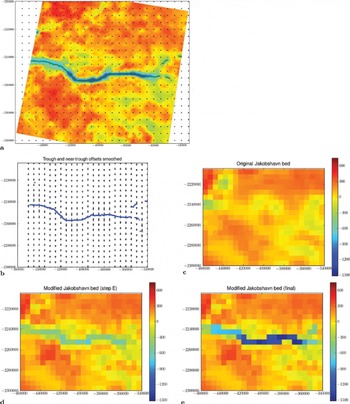
Jakobshavn Isbræ (Ilulissat Ice Stream, terminus at ~69°10' N, 508 W) has been introduced in earlier sections of this paper. The Jakobshavn subregion used for the new bed DEM is -50.2978848 E, 68.6344178 N (lower left map corner) to -47.6419558 E, 69.7275718 N (upper right map corner). The 5 km Jakobshavn bed DEM, created using the jakbeg.algo.v6, and intermediate steps are presented in Figure 3 . The new bed DEM shows a continuous trough with the correct maximal elevation (within the 5 km block) and visually suggests that ice flow will pass unobstructed into the trough and down-valley to the fjord. The canyon rim of the trough is a little rounded, matching the CReSIS observations at this reduced resolution, with a distance-weighted average. The Jakobshavn region of the DEM of Greenland that was used previously is given for comparison in Figure 3d; this grid is based on the topography published in Reference Bamber, Layberry and GogineniBamber and others (2001) and barely shows an indication of Jakobshavn trough near the mouth of the ice stream. Collection of MCoRDS data as part of IceBridge and before IceBridge and application of the new algorithm allowed this advance in bed representation.
Derivation of Jakobshavn Isbræ region 5 km subglacial topography. (a) CReSIS data, gridded by CReSIS (125 m), color scale as in (c–e); 5 km grid nodes are indicated, grid nodes of the trough set are red and trough line is superimposed in green; (b) trough detection and morphologic-stretch algorithm (arrows); (c) original bed (Reference Bamber, Layberry and GogineniBamber and others, 2001); (d) intermediate step, after interpolation with new data and application of morph-stretch algorithm; and (e) final bed with trough integration. Subglacial elevation in m above WGS84. Polar stereographic coordinates (SeaRISE-type). Modified after Reference Herzfeld, Wallin, Leuschen and PlummerHerzfeld and others (2011a).
6.2. Helheim Glacier
Helheim Glacier is located in the Sermilik region of southeastern Greenland at 66.48 N, 388 W. Until 2000, Helheim Glacier was the only glacier in southeast Greenland that still advanced at a time when rapid surface lowering was observed for all other glacial areas in southeast Greenland (Reference KrabillKrabill and others, 1999). Between 2000 and 2005, Helheim Glacier accelerated and retreated twice, with an increase of maximal velocities from 8kma-1 to 11 km a-1 and a total retreat of 7.5 km (Reference Howat, Joughin, Tulaczyk and TulaczykHowat and others, 2005). The map region for the Helheim Glacier trough is -39.1095148 E, 66.3083448 N (lower left map corner) to -37.9975418 E, 66.7578178 N (upper right map corner). A 500 m grid derived by CReSIS is used as a high-resolution data aggregation grid. Helheim Glacier has several branches that join a short distance from the current terminus (see Fig. 4a), which requires a generalization of the trough-search algorithm (see Sections 3 and 5). To automatically identify the location of the several canyon branches, north-south profiles of subglacial topography were analyzed and a 300 m bed elevation threshold used, then east-west profiles were analyzed. The north-south analysis contained all minima needed for derivation of the 5 km trough and resulted in an edge-connected trough set.
Derivation of Helheim Glacier region 5 km subglacial topography. (a) CReSIS data, gridded by CReSIS (500 m); (b) trough detection; (c) trough over high-resolution grid; (d) original bed (Reference Bamber, Layberry and GogineniBamber and others, 2001); (e) intermediate step, after interpolation with new data; and (f) final bed with trough integration. Subglacial elevation in m above WGS84. Polar stereographic coordinates ((a) CReSIS-type, (b–f) SeaRISE-type).
Topography of the mountain ranges and glacier gorges in this region is especially high, as seen in the photograph of neighboring Skagt Glacier gorge in Figure 5, which indicates that subglacial troughs have a rugged morphology as well. This is also reflected in the radar data. The morphologic-stretch algorithm (which has a rounding effect on the trough edges) is not employed, because of the ruggedness of the terrain and the anisotropic pattern of the several bed branches in a relatively small area. Completion of the 5 km bed follows the trough-system algorithm. Trough identification and derivation of the 5km Helheim bed DEM is illustrated in Figure 4.
Skagt Glacier, Sermilik region, East Greenland, July 2005. Photograph by Helmut Mayer and Ute Herzfeld.
6.3. Kangerdlussuaq Glacier
Kangerdlussuaq is a fast-moving outlet in central eastern Greenland. It has a main ice stream that flows south-southeast and several secondary branches. The calculation of the 5km bed for Kangerdlussuaq is carried out as for Helheim Glacier, using a 500m grid derived by CReSIS as an interim high-resolution grid and east–west profiles as dominant for the trough-set identification step, and the lowest point in a neighborhood for elevation association in the trough set. Derivation of the Kangerdlussuaq bed for the map area –33.696239°E, 68.543468°N (lower left map corner) to –32.697422°E, 68.841516°N (upper right map corner) is illustrated in Figure 6. The resultant subarea grid includes the main trough of the Kangerdlussuaq system, the confluence of the main trunk with a branch in the southeast, the lower regions of a small branch that joins in from the west as well as the confluence region with a northwestern branch. Since data coverage ends ~5 km north of the confluence of the northwestern branch and the main trough, the two branches cannot be resolved in the 5 km DEM.
Derivation of Kangerdlussuaq Glacier region 5 km subglacial topography. (a) CReSIS data, gridded by CReSIS (500 m), color scale as in (c); (b) trough detection; (c) trough over high-resolution grid; (d) original bed (Reference Bamber, Layberry and GogineniBamber and others, 2001); (e) intermediate step, after interpolation with new data and application of morph-stretch algorithm; and (f) final bed with trough integration. Subglacial elevation in m above WGS84. Polar stereographic coordinates ((a) CReSIS-type, (b–f) SeaRISE-type).
6.4. Petermann Gletscher
Petermann Gletscher is a large tidewater glacier located in northwest Greenland east of the Nares Strait near 808300 N, 59°30' W which has recently exhibited dramatic changes (Reference Rignot and RignotRignot and Steffen, 2008; Reference Johnson, Muenchow, Falkner and MellingJohnson and others, 2010). The glacier has a 70 km long, 15 km wide long floating tongue, which in August 2010 calved a large ‘ice island’ of 260 km2. Most of the glacier's mass loss occurs through channelized bottom melting (Reference Rignot and RignotRignot and Steffen, 2008). It should be noted that the CReSIS subglacial topography data do not distinguish between floating ice and grounded ice. The small side glaciers entering Petermann in the north (e.g. near-925000/ -390000 and -945000/-390000 in Fig. 7c) are grounded, while the tongue of Petermann is floating in this area. The case of Petermann Glacier emphasizes the importance of including grounding lines in dynamic ice-sheet models (see Reference Herzfeld, Fastook, Greve, McDonald, Wallin and ChenHerzfeld and others, 2012; Reference Greve and HerzfeldGreve and Herzfeld, 2013).
Derivation of Petermann Gletscher region 5 km subglacial topography. (a) CReSIS data, gridded using advanced ordinary kriging (CU Geomath) (500 m); (b) trough detection; (c) trough over high-resolution grid; (d) original bed (Reference Bamber, Layberry and GogineniBamber and others, 2001); (e) intermediate step, after interpolation with new data; and (f) final bed with trough integration. Subglacial elevation (m above WGS84). Polar stereographic coordinates ((a) CReSIS-type, (b–f) SeaRISE-type).
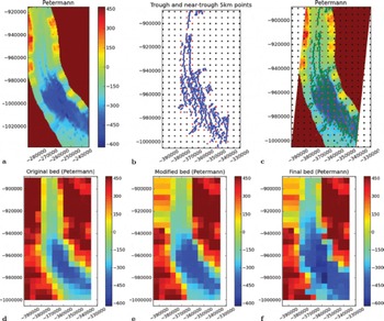
A new Petermann grid is created for the map region -60.4813998 E, 80.0810218 N (lower left map corner) to -59.337720°E, 81.293184°N (upper right map corner). An intermediate-step high-resolution grid at 500 m was derived using advanced kriging with a Gaussian variogram (range 867 m, sill = 3450, nug = 350) and kriging software developed by U.C.H. (see Reference HerzfeldHerzfeld, 1992, Reference Herzfeld2004; Reference Herzfeld, Wallin and StachuraHerzfeld and others, 2011b). The generalized trough-system algorithm was then applied to derive the 5 km grid (Fig. 7).
7. The JakHelKanPet Bed DEM: Relevance to SeaRISE, Availability of the Dataset and Technical Matters
This study is motivated by the need to accurately predict that part of sea-level rise that is caused by mass loss from the Greenland ice sheet, a goal that is shared with SeaRISE, a US-American-led community-organized effort to estimate the upper bound of ice-sheet contributions to sea level in the next 100–200 years (http://websrv.cs.umt.edu/isis/index.php/SeaRISE_Assessment), and ice2sea, a science program that is funded by the European Union Framework-7 scheme to improve projections of the contribution of ice to future sea-level rise (http://www.ice2sea.eu/). Both efforts rely on dynamic ice-sheet models to predict future changes in ice dynamics and in sea level. SeaRISE experiments include several models and change scenarios and are run at 5 km resolution, initially using the bed topography derived by Reference Bamber, Layberry and GogineniBamber and others (2001) (SeaRISE dataset Greenland_ 5km_v0.93.nc) and later an ad hoc bed topography (see Reference BindschadlerBindschadler and others, 2013; Reference NowickiNowicki and others, 2013a). A bed DEM derived in Reference Herzfeld, Wallin, Leuschen and PlummerHerzfeld and others (2011a) that includes (only) Jakobshavn Isbræ has been used in SeaRISE experiments (SeaRISE dataset Greenland_5km_dev1.2.nc) and motivated inclusion of more outlet glacier regions to meet demands of the modeling community. The resultant dataset of the JakHelKanPet Greenland bed DEM (Greenland_5km_JHKP.nc) is available from the ftp site of the first author and from the SeaRISE data wiki (http://websrv.cs.umt.edu/isis/index.php/SeaRISE_Assessment), released in August 2011.
Format and input variables for modeling: Data are output as stacks of several variables in the netcdf format preferred by the modeling community. The bed DEM that results from the analysis described in this paper becomes one layer in the stack of variables. Our algorithm rewrites the entire stack of variables in netcdf, which can be conveniently uploaded into a dynamic ice-sheet model. In addition to the bed elevation, the variables stored in the SeaRISE netcdf format include: latitude, longitude, projected X and Y grid coordinates, isotopes (time and value), sea level (time and value), land-cover mask, surface elevation, thickness, rate of change of the ice surface, measured surface velocity (magnitude, x- and y-components), balance velocity (magnitude), present precipitation, present air temperature, geothermal heat flux, and map projection (http://websrv.cs.umt.edu/isis/index.php/Main_Page).
Projections: CReSIS uses a polar stereographic projection (see Reference SnyderSnyder, 1987) with central meridians at –458 longitude and 908 latitude, and latitude of true scale at 708 N. SeaRISE uses a polar stereographic projection with central meridians at –398 longitude and 908 latitude and latitude of true scale at 71°N. The algorithm used here transforms accordingly. The final JakHelKanPet DEM uses the same projection (the SeaRISE-type projection) for all outlet glacier areas and for the whole Greenland DEM.
8. Application and Validation
Two studies have been conducted to validate that the trough-system algorithm leads to a more realistic representation of Greenland outlet glaciers in dynamic ice-sheet models. The location of high-velocity regions of ice streams in results from dynamic ice-sheet models using the JakHelKanPet DEM matches the location of high-velocity regions indicated by crevassed regions in satellite imagery (Reference Herzfeld, Fastook, Greve, McDonald, Wallin and ChenHerzfeld and others, 2012). A comparison of simulations with velocities derived from observations (according to Reference Joughin, Smith, Howat, Scambos and ScambosJoughin and others, 2010) confirms that the trough-system approach yields a more realistic modeling in the important regions of outlet glaciers (Reference Greve and HerzfeldGreve and Herzfeld, 2013). Remaining limitations are attributed to incapabilities of current whole-Greenland ice-sheet models in handling grounding-line representation.
The influence of Greenland outlet glacier bed topography on results from dynamic ice-sheet models and estimation of sea-level rise has been analyzed in Herzfeld and others (2012). Contrasting different responses of two Greenland ice sheet models (UMISM (the University of Maine Ice Sheet Model; Reference FastookFastook, 1993; Reference Fastook and PrenticeFastook and Prentice, 1994) and SICOPOLIS (SImulation COde for POLythermal Ice Sheets; Greve, 1995, 1997; Reference Greve and HerzfeldGreve and Blatter, 2009)) to two different bed topographies (the Reference Bamber, Layberry and GogineniBamber and others (2001) bed and the JakHelKanPet bed) shows significant differences in modeled surface velocity, basal water production and ice thickness. Modeled ice volumes for the Greenland ice sheet are significantly smaller for the JakHelKanPet bed DEM, and volume losses larger, and hence corresponding predicted sea-level rise is larger (Herzfeld and others, 2012). Because ice flow and ice-stream extent match observations better, it is concluded that results based on simulations using the JakHelKanPet DEM are more realistic. The study demonstrates the importance of correctly representing bed topography of outlet glaciers as a component of ice-sheet modeling and more generally the role of spatial modeling of data specifically as input for dynamic ice-sheet models.
9. Summary and Conclusions
The objective of this paper is to include subglacial troughs of outlet glaciers in a DEM of Greenland bed topography in such a way that those properties of the troughs that affect ice-dynamic modeling of the trough-following outlet glaciers are preserved in the bed-topography DEM. To this end, we derive and apply a mathematical and computational algorithm, termed trough-system algorithm, that (1) preserves subglacial troughs and trough systems with several branches in a generalized cartography, such as a DEM at lower resolution than necessary to resolve the trough system morphology, and (2) results in glacier bed DEMs created with modeling in mind, i.e. designed to preserve those bed characteristics that will affect the dynamics of the modeled variables. The trough-system algorithm employs mathematical concepts from algebraic topology and mathematical morphology to ascertain that locally-maximal depth values are retained in the DEM, the canyon branches are continuous (simply connected), the canyon rims rounded mimicking subglacial erosion and the bed topography is not distorted by the lower-resolution discretization. These properties cannot be achieved by applying a weighted averaging algorithm such as splines or kriging. Advanced ordinary kriging is used (only) for aggregation of data onto high-resolution grids.
The trough-system algorithm is applied to integrate several important outlet glacier systems into a Greenland bed topography DEM. To date, these outlet glacier systems are: Jakobshavn Isbræ, Helheim, Kangerdlussuaq and Petermann glaciers, selected because of their glaciological relevance and because CReSIS has collected MCoRDS radar data with good coverage. The DEM is derived at 5 km resolution as well as in the netcdf format commonly used by the modeling community, so that its application does not require advance of model capabilities. The resultant dataset of the JakHelKanPet bed DEM (Greenland_5km_JHKP.nc; see Fig. 8) is available from the ftp site of the first author and from the SeaRISE data wiki (http://websrv.cs.umt.edu/isis/index.php/SeaRISE_Assessment).
Greenland 5 km subglacial topography. (a) Original bed DEM (Reference Bamber, Layberry and GogineniBamber and others, 2001) (dev0.93 in SeaRISE datasets); (b) final JakHelKanPet bed. Subglacial elevation (m above WGS84). Polar stereographic coordinates (SeaRISE-type). From Herzfeld and others (2012a).
Derivation of the new bed topography DEM meets a need of the dynamic ice-sheet modeling community (see Herzfeld and others, 2012; Reference BindschadlerBindschadler and others, 2013; Reference NowickiNowicki and others, 2013a), especially the SeaRISE community effort to estimate the maximum contribution to sea-level rise from mass loss of the Greenland ice sheet, and results are relevant for the sea-level prediction and cryospheric change components of the IPCC's Fifth Assessment Report (2012). The goal of the algorithm is to bridge between data observation and modeling, and this goal has influenced the philosophy driving selection and derivation of computational methods. While instrumentation may be improved, more data may need to be collected and ice-sheet model resolutions may need to be increased in the future, the role of such an algorithm is to be able to obtain better results from presently collected data with current modeling techniques.
9.1. Discussion
The philosophy of the approach described here is to derive bed topographic grids only from bed topographic data and mathematical concepts. In contrast, several recent studies employ the principle of mass conservation to improve DEMs of bed topography (Reference Farinotti, Huss, Bauder, Funk and FunkFarinotti and others, 2009; Reference Larour, Seroussi, Morlighem and MorlighemLarour and others, 2012; Reference MorlighemMorlighem and others, 2013), which requires use of ice-surface velocity as an auxiliary dataset. The theory of the mass-conservation method for reconstruction of ice thickness (Reference RasmussenRasmussen, 1988) expects information on velocity at depth, but for lack of observations velocity at depth is commonly extrapolated from velocity at the surface (Reference RasmussenRasmussen, 1988; Reference Farinotti, Huss, Bauder, Funk and FunkFarinotti and others, 2009; Reference Larour, Seroussi, Morlighem and MorlighemLarour and others, 2012; Reference MorlighemMorlighem and others, 2013). The extrapolation uses assumptions about continuity of velocity change with depth, which limit the types of ice flow that can be analyzed. For example, the velocity of a surge-type glacier changes over time, hence a different bed may result using different velocity observations from different time points. A continuity assumption of velocity change with depth is unlikely to hold for a surge-type glacier. Considering that ice-dynamic models derive surface velocity as one of their main resultant variables, using surface velocity to invert for bed topography may lead to circuitous conclusions on velocity and accelerations of glaciers in ice-dynamic models and preclude investigations of complex accelerations and englacial processes. For these reasons, an approach that uses only ice-thickness observations/depth data is preferable. In the trough-system algorithm, the mathematical concept of simple-connectedness of the subglacial trough systems ascertains that ice flow is not inhibited and that ice that enters a trough or trough system at its source(s) will proceed through the trough system to the glacier terminus.
9.2. Generalizations
Since the trough-system algorithm is sufficiently generalized, it can be applied to also include other areas, that are planned to be surveyed as part of Operation IceBridge and other campaigns. This is currently work in progress. The trough-system algorithm can be applied at any gridscale, to meet requirements of models that can handle higher-resolution grids. There are ice-dynamic models that solve the problem of outlet-glacier representation differently (Reference Larour, Seroussi, Morlighem and MorlighemLarour and others, 2012) by increasing resolution for ice-stream regions, but most models do not have this capability. As dynamic ice-sheet modeling capabilities may improve to utilize variable-scale grids, the trough-bed algorithm can also be used to create grids with location-dependent scales. Furthermore, the trough-bed algorithm makes it possible to use new data collected over outlet glacier regions, derive improved trough system topographies for subregions and integrate these in any subglacial base topography outside of outlet glacier regions; a component of the algorithm facilitates seamless integration.
Acknowledgements
Analysis of CReSIS data and derivation of the Greenland bed topography DEM by U.C.H., B.W.M. and B.F.W. has been supported by NASA Cryospheric Sciences Awards NNX09A083G ‘Spatial Ice Surface Roughness – Scale-Dependent Analyses of Ice Surfaces and Implications for Cryospheric Sciences and Satellite Altimetry (in Particular, for ICESat and ICESat-2)’ and NNX11AP39G ‘Spatial Modeling of Greenland Bed Topography as Input for Dynamic Ice Sheet Models: A Contribution to SeaRISE’ (principal investigator U.C. Herzfeld). Assistance with data analysis by P.A.C. and B.W.M. was supported by the University of Colorado Boulder Undergraduate Research Opportunity Program. Data and/or data products from CReSIS were generated with support from US National Science Foundation grant ANT-0424589 and NASA grant NNX10AT68G. MCoRDS 2009 and 2010 data were collected as part of NASA Operation IceBridge. Field observations and photographs were collected during Greenland field projects as part of DFG He1547/4, He1547/7, He1547/8 and Ma2486/1 supported by Deutsche Forschungsgemeinschaft. All this support is gratefully acknowledged. Thanks to Ralf Greve, James Fastook, Robert Bindschadler, Sophie Nowicki and the SeaRISE group for motivating U.C.H. to include HelKanPet in the Greenland bed DEM and to Joel Plummer for contributions to processing of Jakobshavn Isbræ radar data. Thanks to David Braaten for editing Annals of Glaciology 55(67).


