





1. Introduction
The stability properties of a sheared, density-stratified environment is significant because unstable shear layers can lead to nonlinear overturning waves propagating along the density interface producing turbulence and mixing (Carpenter, Balmforth & Lawrence Reference Carpenter, Balmforth and Lawrence2010), and ultimately atomisation in two-phase flows (Lasheras, Villermaux & Hopfinger Reference Lasheras, Villermaux and Hopfinger1998; Lefebvre & McDonell Reference Lefebvre and McDonell2017). Understanding when and where turbulence and mixing occur in shear layers is important in engineering systems such as fuel mixing in combustion engines (Juniper & Candel Reference Juniper and Candel2003; Sirignano Reference Sirignano2021), potentially making them more efficient; in the aerospace and marine industry where shear layers generate drag and noise, they can also control turbulence, via methods such as compliant surfaces, leading to improved performance and fuel efficiency (Weilgart Reference Weilgart2018; Poole & Turner Reference Poole and Turner2023); and environmental flows where the mixing of weather patterns or pollutants can affect climate modelling and environmental monitoring (Peltier & Caulfield Reference Peltier and Caulfield2003; Caulfield Reference Caulfield2021). Calculating the stability of such shear layers has a long history going back to Helmholtz (Reference Helmholtz1868) and Kelvin (Reference Kelvin1871) for two-dimensional homogeneous and stratified shear layers, respectively. Since these initial works, various authors have considered variations to these problems, making the problem more complex, but each time focusing on understanding the basic instability mechanism and how it might be exploited and controlled.
In this paper our focus is on calculating the transition point from convective to absolutely unstable flows. A convectively unstable flow is one where instability modes grow and propagate away from the source of the disturbance (either upstream or downstream), while an absolutely unstable flow has instability modes that propagate both upstream and downstream from the disturbance source. An important feature of an absolute instability is that it can lead to a global instability that can dominate and fill the whole flow domain, and in fact, for a strictly parallel flow, an absolute instability is equivalent to a global instability. Huerre & Monkewitz (Reference Huerre and Monkewitz1985) was the first significant study of absolute instability in the hydrodynamic context, showing that the unconfined homogeneous shear layer was absolutely unstable. This work was extended by Triantafyllou (Reference Triantafyllou1994) to include a discontinuous step in density between the two layers. The initial work by Huerre & Monkewitz (Reference Huerre and Monkewitz1985) has inspired a huge array of studies on this problem, producing a vast literature. However, the effect of flow asymmetries on the stability of a stratified shear layer has received little attention, but is of interest in engineering shear flows including high-speed jets.
The shear layer we consider consists of two fluids flowing parallel to the $x$
axis, is two-dimensional, with dimensional velocities
$x$
axis, is two-dimensional, with dimensional velocities $U_1^*\boldsymbol{e}_x$
and
$U_1^*\boldsymbol{e}_x$
and $U_2^*\boldsymbol{e}_x$
far from the shear layer, and we non-dimensionalise our problem with the typical velocity scale
$U_2^*\boldsymbol{e}_x$
far from the shear layer, and we non-dimensionalise our problem with the typical velocity scale $(U_1^*+U_2^*)/{2}$
. This gives us a dimensionless basic velocity profile
$(U_1^*+U_2^*)/{2}$
. This gives us a dimensionless basic velocity profile $U(y)\boldsymbol{e}_x$
of the form
$U(y)\boldsymbol{e}_x$
of the form
 \begin{equation} U(y)=1+rf(y), \end{equation}
where $y$
is a variable in the cross-stream direction,
$y$
is a variable in the cross-stream direction, $\lim _{y\to \pm \infty }f(y)=\pm 1$
and
$\lim _{y\to \pm \infty }f(y)=\pm 1$
and
 \begin{align} r=\frac {U_1^*-U_2^*}{U_1^*+U_2^*} \end{align}
is the shear flow parameter. Note that in this formulation we remain in the fixed inertial frame of reference, rather than converting to a moving frame. This is because the focus of this work is on classifying absolutely and convectively unstable flow parameter regimes, and this distinction would become more confusing if the parameter-dependent speed of the moving frame needs to be taken into account. In the fixed inertial frame, an absolute instability is an instability that has zero group velocity. The two fluids have densities $\rho _1$
and
$\rho _1$
and $\rho _2$
with the density ratio defined by
$\rho _2$
with the density ratio defined by $S=\rho _2/\rho _1\gt 1$
, such that the flow is stably stratified. The dimensionless position variables
$S=\rho _2/\rho _1\gt 1$
, such that the flow is stably stratified. The dimensionless position variables $(x,y)$
are non-dimensionalised on a convenient measure of the shear layer thickness,
$(x,y)$
are non-dimensionalised on a convenient measure of the shear layer thickness, $L$
. When
$L$
. When $|r|\lt 1$
,
$|r|\lt 1$
, $U_1^*$
and
$U_1^*$
and $U_2^*$
have the same sign, we call this a co-flow shear layer, while when
$U_2^*$
have the same sign, we call this a co-flow shear layer, while when $|r|\gt 1$
,
$|r|\gt 1$
, $U_1^*$
and
$U_1^*$
and $U_2^*$
are of opposite sign and we call this a counterflow shear layer. The flow is a parallel flow, i.e. the base flow only depends on the cross-stream variable
$U_2^*$
are of opposite sign and we call this a counterflow shear layer. The flow is a parallel flow, i.e. the base flow only depends on the cross-stream variable $y$
, and so any absolute instability also implies a global instability. For
$y$
, and so any absolute instability also implies a global instability. For $f(y)=\tanh (y/2)$
, Huerre & Monkewitz (Reference Huerre and Monkewitz1985) found that for strong counter flows, the flow is absolutely unstable, and convectively unstable otherwise, with the transition at
$f(y)=\tanh (y/2)$
, Huerre & Monkewitz (Reference Huerre and Monkewitz1985) found that for strong counter flows, the flow is absolutely unstable, and convectively unstable otherwise, with the transition at $r=1.315$
. However, Huerre & Monkewitz (Reference Huerre and Monkewitz1985) were only considering an unconfined shear layer, and Healey (Reference Healey2009) showed that confinement of the shear layer between two parallel plates is significant to the absolute instability properties of the flow, with the biggest absolute instability effects produced by asymmetric confinement.
$r=1.315$
. However, Huerre & Monkewitz (Reference Huerre and Monkewitz1985) were only considering an unconfined shear layer, and Healey (Reference Healey2009) showed that confinement of the shear layer between two parallel plates is significant to the absolute instability properties of the flow, with the biggest absolute instability effects produced by asymmetric confinement.
The mathematical justification showing the importance of confinement comes from the challenge of applying spatio-temporal stability analysis together with the Briggs method (Briggs Reference Briggs1964). In this theory the initial value problem is solved using an impulse disturbance and taking Fourier transforms in $x$
and Laplace transforms in time
$x$
and Laplace transforms in time $t$
. The resulting solution is hence an inverse Fourier–Laplace transform, which by using the method of steepest descent in the large
$t$
. The resulting solution is hence an inverse Fourier–Laplace transform, which by using the method of steepest descent in the large $t$
limit can be written as a Fourier integral over
$t$
limit can be written as a Fourier integral over $\alpha$
, the streamwise wavenumber. The absolute instability properties can then be determined by deforming the Fourier inversion contour through special saddle points in the complex
$\alpha$
, the streamwise wavenumber. The absolute instability properties can then be determined by deforming the Fourier inversion contour through special saddle points in the complex $\alpha$
plane that link both upstream and downstream propagating wavepackets. The dominant saddle is the one with the largest
$\alpha$
plane that link both upstream and downstream propagating wavepackets. The dominant saddle is the one with the largest $\textrm {Im}(\omega )$
, where
$\textrm {Im}(\omega )$
, where $\omega$
is the disturbance angular frequency, and is known as a pinch point, when we use the wave-form convention
$\omega$
is the disturbance angular frequency, and is known as a pinch point, when we use the wave-form convention $\exp (\textrm {i}(\alpha x-\omega t))$
in (2.2)–(2.4). For unbounded shear layers, with exponential decay as
$\exp (\textrm {i}(\alpha x-\omega t))$
in (2.2)–(2.4). For unbounded shear layers, with exponential decay as $y\to \pm \infty$
, the dominant saddle lies in the quadrant
$y\to \pm \infty$
, the dominant saddle lies in the quadrant $\textrm {Re}(\alpha )\gt 0$
,
$\textrm {Re}(\alpha )\gt 0$
, $\textrm {Im}(\alpha )\lt 0$
, and a branch cut lies along the negative imaginary
$\textrm {Im}(\alpha )\lt 0$
, and a branch cut lies along the negative imaginary $\alpha$
axis. However, when the flow is confined by rigid plates, the decaying solution is replaced by a no-penetration condition at the plate (for inviscid flows) that generates an infinite number of discrete poles and saddle points close to the imaginary
$\alpha$
axis. However, when the flow is confined by rigid plates, the decaying solution is replaced by a no-penetration condition at the plate (for inviscid flows) that generates an infinite number of discrete poles and saddle points close to the imaginary $\alpha$
axis. The addition of these additional saddle points makes identifying the dominant pinch point challenging, but Healey (Reference Healey2009) showed that these saddles can become the dominant saddle under certain flow conditions. Healey also showed, building on his works on the rotating disc boundary layer (Healey Reference Healey2006a
,
Reference Healeyb
, Reference Healey2007) that confinement of shear layers can cause modes that are convectively unstable in the cross-flow direction,
$\alpha$
axis. The addition of these additional saddle points makes identifying the dominant pinch point challenging, but Healey (Reference Healey2009) showed that these saddles can become the dominant saddle under certain flow conditions. Healey also showed, building on his works on the rotating disc boundary layer (Healey Reference Healey2006a
,
Reference Healeyb
, Reference Healey2007) that confinement of shear layers can cause modes that are convectively unstable in the cross-flow direction, $y$
, to become absolutely unstable modes. This occurs when the dominant mode in the unbounded problem crosses the imaginary
$y$
, to become absolutely unstable modes. This occurs when the dominant mode in the unbounded problem crosses the imaginary $\alpha$
axis to a region where the wavepacket grows exponentially in a direction with a cross-flow direction component, but the rigid plate enforces a zero boundary condition and, thus, the mode travels back to the shear layer, setting up the absolute instability. This phenomena also allows the absolute instability to persist even when the plate is moved arbitrarily far from the shear layer. This same behaviour is seen for other flows such as planar jets and wakes (Yu & Monkewitz Reference Yu and Monkewitz1990; Taylor & Peake Reference Taylor and Peake1999; Juniper Reference Juniper2006, Reference Juniper2007, Reference Juniper2008) and swirling jets (Lim & Redekopp Reference Lim and Redekopp1998; Healey Reference Healey2008).
$\alpha$
axis to a region where the wavepacket grows exponentially in a direction with a cross-flow direction component, but the rigid plate enforces a zero boundary condition and, thus, the mode travels back to the shear layer, setting up the absolute instability. This phenomena also allows the absolute instability to persist even when the plate is moved arbitrarily far from the shear layer. This same behaviour is seen for other flows such as planar jets and wakes (Yu & Monkewitz Reference Yu and Monkewitz1990; Taylor & Peake Reference Taylor and Peake1999; Juniper Reference Juniper2006, Reference Juniper2007, Reference Juniper2008) and swirling jets (Lim & Redekopp Reference Lim and Redekopp1998; Healey Reference Healey2008).
When stratified shear flows are observed in laboratory experiments (Koop & Browand Reference Koop and Browand1979; Lawrence, Browand & Redekopp Reference Lawrence, Browand and Redekopp1991), they often exhibit some form of asymmetry. This asymmetry can take the form of asymmetric confinement above or below the shear layer, a displaced density interface from the centre of the shear layer or asymmetric velocity profiles. In this work we focus on asymmetric confinement and a displaced density interface. For an homogeneous shear layer, Healey (Reference Healey2009) showed that for temporal instabilities, asymmetric confinement is the most stable configuration, followed by symmetric confinement, semi-confinement and then unconfined flows. However, Healey showed that, for the absolute instability, the asymmetric confined configuration is the most unstable. The series of experiments by Matas (Reference Matas2015), Matas, Delon & Cartellier (Reference Matas, Delon and Cartellier2018) and Bozonnet et al. (Reference Bozonnet, Matas, Balarac and Desjardins2022) for an air–water shear layer confirm the findings of Healey (Reference Healey2009) by showing that asymmetric confinement can generate an absolute instability in flow regimes, which, when unconfined, are convectively unstable. Stratified shear layers in the ocean are not immediately applicable to the results in this paper because in these cases the density stratification between the upper and lower oceans is about $S\approx 1$
. However, what is significant is that in these flows the effect of displacing the shear interface away from the centre of the shear layer has been studied. Varying the location of this point generates significant differences in the form of the nonlinear waves that are generated on the interface surface (Lawrence et al. Reference Lawrence, Browand and Redekopp1991; Caulfield et al. Reference Caulfield, Peltier, Yoshida and Ohtani1995; Carpenter et al. Reference Carpenter, Balmforth and Lawrence2010), and Danyi (Reference Danyi2018) found that displacing the mean density position with respect to the position of the shear layer can destabilise the flow, even if the stratification is a stable stratification. In this paper our results will focus on the effect of varying the density interface position in high-speed jet flows with
$S\approx 1$
. However, what is significant is that in these flows the effect of displacing the shear interface away from the centre of the shear layer has been studied. Varying the location of this point generates significant differences in the form of the nonlinear waves that are generated on the interface surface (Lawrence et al. Reference Lawrence, Browand and Redekopp1991; Caulfield et al. Reference Caulfield, Peltier, Yoshida and Ohtani1995; Carpenter et al. Reference Carpenter, Balmforth and Lawrence2010), and Danyi (Reference Danyi2018) found that displacing the mean density position with respect to the position of the shear layer can destabilise the flow, even if the stratification is a stable stratification. In this paper our results will focus on the effect of varying the density interface position in high-speed jet flows with $S\geqslant 1$
.
$S\geqslant 1$
.
In this paper we derive the governing equations in § 2 and examine the neutral curves for the temporal stability for confined shear layers in § 3. In § 4 we derive the long-wavelength dispersion relations for comparison with full numerical results in § 5 for symmetrically confined shear layers and § 6 for asymmetrically confined shear layers. In § 6 we also consider the absolute instability of semi-confined shear layers (asymmetrically confined by a single plate) and give a simple mechanism for the stability hierarchy identified. Comparison of the results in §§ 5 and 6 for a continuous density profile is considered in § 7, confirming the robustness of the results previously identified. Conclusions are given in § 8.
Schematic of the shear layer problem we consider. The density stratification is assumed to be stable, so $S\geq 1$
and the shear rate,
$S\geq 1$
and the shear rate, $r$
, can be positive or negative.
$r$
, can be positive or negative.

2. Governing equations
The shear layer problem considered in figure 1 is assumed to be inviscid and irrotational and, thus, the governing equations are the two-dimensional non-dimensionalised Euler equations
 \begin{equation} \frac {\partial \boldsymbol{u}}{\partial t}+\boldsymbol{u}\boldsymbol{\cdot }\boldsymbol{\nabla }\boldsymbol{u}=-\frac {1}{{\rho }}\boldsymbol{\nabla }\widehat {p}-F^{-2}\boldsymbol{e}_y,\,\,\,\,\,\boldsymbol{\nabla }\boldsymbol{\cdot }\boldsymbol{u}=0,\,\,\,\,\,{\frac {\partial \rho }{\partial t}+\boldsymbol{u}\boldsymbol{\cdot }\boldsymbol{\nabla }\rho =0}, \end{equation}
where $F=(U^*_1+U^*_2)/(2\sqrt {gL})$
is the Froude number,
$F=(U^*_1+U^*_2)/(2\sqrt {gL})$
is the Froude number, $\boldsymbol{e}_y$
is a unit vector in the
$\boldsymbol{e}_y$
is a unit vector in the $y$
direction and
$y$
direction and $g$
is the gravitational constant. Here
$g$
is the gravitational constant. Here $\boldsymbol{u}=(\widehat {u},\widehat {v})$
are the velocity components in the
$\boldsymbol{u}=(\widehat {u},\widehat {v})$
are the velocity components in the $x$
and
$x$
and $y$
directions, and
$y$
directions, and $\widehat {p}$
is the pressure. The function
$\widehat {p}$
is the pressure. The function $\widehat {S}(y)$
is the non-dimensional density profile and is assumed to vary only in the cross-flow direction. The flow is confined above and below by rigid parallel plates at
$\widehat {S}(y)$
is the non-dimensional density profile and is assumed to vary only in the cross-flow direction. The flow is confined above and below by rigid parallel plates at $y=h_1$
and
$y=h_1$
and $y=-h_2$
.
$y=-h_2$
.
The form of the governing stability equations come from seeking two-dimensional normal-mode disturbances to the basic parallel velocity profile $\boldsymbol{u}=U(y)\boldsymbol{e}_x$
of the form
$\boldsymbol{u}=U(y)\boldsymbol{e}_x$
of the form
 \begin{align} \boldsymbol{u}=(\widehat {u}(x,y,t),\widehat {v}(x,y,t))&=(U(y),0)+\widehat {\delta }(u(y),v(y))\exp \left [ \textrm {i}(\alpha x-\omega t)\right ],\end{align}
 \begin{align} \widehat {p}(x,y,t)&= P_0-\int \widehat {S}(y)F^{-2}\,{\textrm {d}} y+\widehat {\delta } p(y)\exp \left [\textrm {i}(\alpha x-\omega t)\right ],\end{align}
 \begin{align} \rho (x,y,t)&= \widehat {S}(y)+\widehat {\delta }\sigma (y)\exp \left [\textrm {i}(\alpha x-\omega t)\right ],\end{align}
where $0\lt \widehat {\delta }\ll 1$
is a small parameter that allows for linearisation and
$0\lt \widehat {\delta }\ll 1$
is a small parameter that allows for linearisation and $P_0$
is a constant. The disturbances are wave-like disturbances with wavenumber
$P_0$
is a constant. The disturbances are wave-like disturbances with wavenumber $\alpha$
and angular frequency
$\alpha$
and angular frequency $\omega =\alpha c$
, where
$\omega =\alpha c$
, where $c$
is the phase speed. Substituting these forms into (2.1) and linearising leads to the system of equations
$c$
is the phase speed. Substituting these forms into (2.1) and linearising leads to the system of equations
 \begin{align} \textrm {i} \alpha u+v' &= 0, \end{align}
 \begin{align} -\textrm {i}\omega u+\textrm {i}\alpha U u+U'v &= -\textrm {i}\alpha \frac {p}{\widehat {S}},\end{align}
 \begin{align} -\textrm {i}\omega v+\textrm {i}\alpha U v &= -\frac {p'}{\widehat {S}}-F^{-2}\frac {{\sigma }}{\widehat {S}},\end{align}
 \begin{align} -\textrm {i}\omega \sigma +\textrm {i}\alpha U\sigma +v\widehat {S}' &= 0, \end{align}
where the dash denotes a derivative with respect to $y$
. Eliminating the quantities
$y$
. Eliminating the quantities $u$
,
$u$
, $\sigma$
and
$\sigma$
and $p$
from these equations leads to a modified Taylor–Goldstein equation
$p$
from these equations leads to a modified Taylor–Goldstein equation
 \begin{equation} (\alpha U-\omega )(v''-\alpha ^2v)-\alpha U''v+\frac {\widehat {S}'}{\widehat {S}}\left [ (\alpha U-\omega )v'-\alpha U' v-\frac {\alpha ^2F^{-2}}{(\alpha U-\omega )}v\right ]=0, \end{equation}
with the inertia terms retained (Drazin & Reid Reference Drazin and Reid1981; Drazin Reference Drazin2002). Here $F^{-2}\widehat {S}'/\widehat {S}$
is the Richardson number, a measure of the buoyancy to shear in the system. This equation is solved with the appropriate boundary conditions, which, for
$F^{-2}\widehat {S}'/\widehat {S}$
is the Richardson number, a measure of the buoyancy to shear in the system. This equation is solved with the appropriate boundary conditions, which, for $h_1$
or
$h_1$
or $h_2$
finite, are
$h_2$
finite, are
 \begin{equation} v(h_1)=v(-h_2)=0, \end{equation}
while, for $h_1$
or
$h_1$
or $h_2$
infinite,
$h_2$
infinite,
 \begin{equation} v'(h_1)+\alpha v(h_1)=v'(-h_2)-\alpha v(-h_2)=0, \end{equation}
gives the correct exponential decay at $y=\pm \infty$
, when
$y=\pm \infty$
, when $\textrm {Re}(\alpha )\gt 0$
. It should also be noted that in this case we also require the wave to be unstable, i.e.
$\textrm {Re}(\alpha )\gt 0$
. It should also be noted that in this case we also require the wave to be unstable, i.e. $\omega _i\gt 0$
. In the case when the mode decays in time
$\omega _i\gt 0$
. In the case when the mode decays in time $\omega _i\lt 0$
, then the causal solutions could involve exponential growth in the far field (Le Dizès & Billant Reference Le Dizès and Billant2009; Riedinger, Le Dizès & Meunier Reference Riedinger, Le Dizès and Meunier2010; Zuccoli, Brambley & Barkley Reference Zuccoli, Brambley and Barkley2024). When using (2.11) in numerical calculations,
$\omega _i\lt 0$
, then the causal solutions could involve exponential growth in the far field (Le Dizès & Billant Reference Le Dizès and Billant2009; Riedinger, Le Dizès & Meunier Reference Riedinger, Le Dizès and Meunier2010; Zuccoli, Brambley & Barkley Reference Zuccoli, Brambley and Barkley2024). When using (2.11) in numerical calculations, $h_1$
and
$h_1$
and $h_2$
need to be chosen large enough such that the eigenmode is in the correct exponential decay regime, and we find that a value of
$h_2$
need to be chosen large enough such that the eigenmode is in the correct exponential decay regime, and we find that a value of $h_1=h_2=20$
is sufficient to guarantee this for the results in this paper.
$h_1=h_2=20$
is sufficient to guarantee this for the results in this paper.
In §§ 3–6 we consider a discontinuous density profile that consists of a jump in density at $y=d$
, and so in this case
$y=d$
, and so in this case $\widehat {S}(y)$
takes the form
$\widehat {S}(y)$
takes the form
 \begin{equation} \widehat {S}(y)=\left \{\begin{array}{ll} 1, & y\geq d, \\ S, & y\lt d, \end{array} \right . \end{equation}
with $S\geqslant 1$
so that the stratification is stable. This profile is a model for the scenario of two immiscible fluids in the shear layer, such as the breakup of liquid–liquid jets (Kitamura, Mishima & Takahashi Reference Kitamura, Mishima and Takahashi1982; Richards, Lenhoff & Beris Reference Richards, Lenhoff and Beris1994; Homma et al. Reference Homma, Koga, Matsumoto, Song and Tryggvason2006) or the breakup of liquid jets in a coaxial injector (Juniper & Candel Reference Juniper and Candel2003; Juniper Reference Juniper2006). In this case we require two jump conditions at
$S\geqslant 1$
so that the stratification is stable. This profile is a model for the scenario of two immiscible fluids in the shear layer, such as the breakup of liquid–liquid jets (Kitamura, Mishima & Takahashi Reference Kitamura, Mishima and Takahashi1982; Richards, Lenhoff & Beris Reference Richards, Lenhoff and Beris1994; Homma et al. Reference Homma, Koga, Matsumoto, Song and Tryggvason2006) or the breakup of liquid jets in a coaxial injector (Juniper & Candel Reference Juniper and Candel2003; Juniper Reference Juniper2006). In this case we require two jump conditions at $y=d$
to ensure we have continuity of the normal displacement of the fluids and the continuity of pressure at the density interface, which are given by
$y=d$
to ensure we have continuity of the normal displacement of the fluids and the continuity of pressure at the density interface, which are given by
 \begin{equation} \left [\frac {v}{\alpha U-\omega } \right ]_{y=d}=0\,\,\,\,\textrm {and}\,\,\,\,\left [\widehat {S}\left \{(\alpha U-\omega )v'-\alpha U'v-\frac {\alpha ^2 F^{-2}}{(\alpha U-\omega )}v\right \}\right ]_{y=d}=0, \end{equation}
where $[\boldsymbol{\cdot }]_{y=d}\equiv \lim _{y\to d^+}[\boldsymbol{\cdot }]-\lim _{y\to d^-}[\boldsymbol{\cdot }]$
(Pouliquen, Chomaz & Huerre Reference Pouliquen, Chomaz and Huerre1994; Schmid & Henningson Reference Schmid and Henningson2001).
$[\boldsymbol{\cdot }]_{y=d}\equiv \lim _{y\to d^+}[\boldsymbol{\cdot }]-\lim _{y\to d^-}[\boldsymbol{\cdot }]$
(Pouliquen, Chomaz & Huerre Reference Pouliquen, Chomaz and Huerre1994; Schmid & Henningson Reference Schmid and Henningson2001).
The form of the basic shear layer flow we consider is given by (1.1). The flow shear rate, $r$
, can be positive or negative and this change corresponds to the faster stream being in the lighter or heavier fluid, respectively. In this paper we present new theoretical and numerical results on the temporal stability of a general shear layer where
$r$
, can be positive or negative and this change corresponds to the faster stream being in the lighter or heavier fluid, respectively. In this paper we present new theoretical and numerical results on the temporal stability of a general shear layer where $f$
in (1.1) is a general anti-symmetric function with the required properties, and illustrate these findings specifically for the tanh shear layer where
$f$
in (1.1) is a general anti-symmetric function with the required properties, and illustrate these findings specifically for the tanh shear layer where
 \begin{equation} f(y)=\tanh \left (\frac {y}{2}\right ). \end{equation}
The absolute instability results will solely be focused on the tanh shear layer.
In the results we present our interest is in considering a fixed anti-symmetric velocity profile (1.1) with $f(y)=-f(-y)$
for varying
$f(y)=-f(-y)$
for varying $r$
, but then breaking the remaining symmetry of the flow by considering both asymmetric confinement
$r$
, but then breaking the remaining symmetry of the flow by considering both asymmetric confinement $h_1\neq h_2$
and by considering a density jump that is asymmetric about
$h_1\neq h_2$
and by considering a density jump that is asymmetric about $y=0$
, i.e.
$y=0$
, i.e. $d\neq 0$
in (2.12). This second case has been observed in the ocean scenario (Anni & Farmer Reference Anni and Farmer1988; Wesson & Gregg Reference Wesson and Gregg1994; Yoshida et al. Reference Yoshida, Ohtani, Nishida and Linden1998; Tedford et al. Reference Tedford, Carpenter, Pawlowicz, Pieters and Lawrence2009) as well as in the laboratory (Koop & Browand Reference Koop and Browand1979; Lawrence et al. Reference Lawrence, Browand and Redekopp1991).
$d\neq 0$
in (2.12). This second case has been observed in the ocean scenario (Anni & Farmer Reference Anni and Farmer1988; Wesson & Gregg Reference Wesson and Gregg1994; Yoshida et al. Reference Yoshida, Ohtani, Nishida and Linden1998; Tedford et al. Reference Tedford, Carpenter, Pawlowicz, Pieters and Lawrence2009) as well as in the laboratory (Koop & Browand Reference Koop and Browand1979; Lawrence et al. Reference Lawrence, Browand and Redekopp1991).
2.1. Potential effects of viscosity
In this work we have considered a shear layer model where viscosity is neglected. In a truly inviscid problem this is a valid assumption, but we briefly consider the consequences of the presented results when a small, finite viscosity is considered. One major feature missing in the inviscid problem is boundary layers at the plates. Typically boundary layer instabilities are weaker than shear layer instabilities, so if the boundary layers at the plate are thin, which they usually are in large-Reynolds-number shear flows such as those we are interested in, their influence should be minimal. Rienstra & Darau (Reference Rienstra and Darau2011) showed that, for a simple piecewise-linear boundary layer next to an impedance wall, the most absolutely unstable scenario is the inviscid, zero thickness boundary layer. A stabilising effect on the absolute instability for moderate Reynolds numbers was also found for jets and wakes by Juniper, Tammisola & Lundell (Reference Juniper, Tammisola and Lundell2011) and Tammisola et al. (Reference Tammisola, Lundell, Schlatter, Wehrfritz and Söderberg2011) and for a swirling jet flow by Tammisola & Juniper (Reference Tammisola and Juniper2016). They concluded that, for strong symmetric confinements, the boundary layers at the plates can begin to interfere with the shear layers, leading to an enhanced stabilisation of the flow. In the current work the majority of the confinements we consider are weak and moderate, hence, we expect our results to be relevant for large- and moderate-Reynolds-number flows.
The addition of weak viscosity would also lead to a diffusion of mass and momentum between the two fluids at the interface by imposing continuous tangential stress. This effect would act to smooth out the density jump at the interface, as well as modifying both it and the velocity profile, into asymmetric configurations that are no longer anti-symmetric about $y=0$
. The smoothed purely anti-symmetric form of the density profile is considered in § 7, but the asymmetric forms are not considered, despite them being observed in experimental set-ups (Ouro, Muhawenimana & Wilson Reference Ouro, Muhawenimana and Wilson2019). Healey (Reference Healey2009) showed that, for a homogeneous shear layer, an asymmetric velocity profile can be destabilising in a symmetrically confined system, but the confinement had to be strong and the asymmetric velocity profile carefully chosen to achieve this. Thus, asymmetric confinement in the homogeneous case has a much more significant effect on the absolute instability and we expect this to also be the case for the stratified problem we consider here.
$y=0$
. The smoothed purely anti-symmetric form of the density profile is considered in § 7, but the asymmetric forms are not considered, despite them being observed in experimental set-ups (Ouro, Muhawenimana & Wilson Reference Ouro, Muhawenimana and Wilson2019). Healey (Reference Healey2009) showed that, for a homogeneous shear layer, an asymmetric velocity profile can be destabilising in a symmetrically confined system, but the confinement had to be strong and the asymmetric velocity profile carefully chosen to achieve this. Thus, asymmetric confinement in the homogeneous case has a much more significant effect on the absolute instability and we expect this to also be the case for the stratified problem we consider here.
3. Temporal stability of confined shear layers
The theoretical results we present here are concerned with the position of the neutral curve as confinement parameters are varied for fixed system parameters $S,\,d,\,r,\,F^{-2}$
. Along the neutral curve
$S,\,d,\,r,\,F^{-2}$
. Along the neutral curve $c={\omega /\alpha }{=}c_r+\textrm {i} c_i$
is purely real (
$c={\omega /\alpha }{=}c_r+\textrm {i} c_i$
is purely real ( $c_i=0$
) and we seek the value of
$c_i=0$
) and we seek the value of $\alpha \in \mathbb{R}$
at the point where
$\alpha \in \mathbb{R}$
at the point where $c_i$
first equals
$c_i$
first equals $0$
. Inside the neutral curves
$0$
. Inside the neutral curves $c\in \mathbb{C}$
and to determine information about growth rates,
$c\in \mathbb{C}$
and to determine information about growth rates, $c_i$
, for such disturbances requires a numerical solution of (2.9).
$c_i$
, for such disturbances requires a numerical solution of (2.9).
Before going on to explore theoretical results on the temporal stability neutral curve of these stratified shear flows, we motivate our analysis by considering the global temporal eigenvalue structure, inside the neutral curve ( $c_i\neq 0$
), for the tanh shear layer for the value
$c_i\neq 0$
), for the tanh shear layer for the value $\alpha =0.2$
and
$\alpha =0.2$
and $r=1$
in figure 2 for the cases
$r=1$
in figure 2 for the cases $S=1$
and
$S=1$
and $S=5$
(panel a) with
$S=5$
(panel a) with $(F^{-2},d)=(0,1)$
(panel b),
$(F^{-2},d)=(0,1)$
(panel b), $(F^{-2},d)=(0,-1)$
(panel c),
$(F^{-2},d)=(0,-1)$
(panel c), $(F^{-2},d)=(0.075,1)$
(panel d). In each case the flow is symmetrically confined with
$(F^{-2},d)=(0.075,1)$
(panel d). In each case the flow is symmetrically confined with $h_1=h_2=10$
. The numerical scheme for this calculation, solving (2.9), is based on collocation with Chebyshev polynomials and is given in § A of the supplementary material. The density ratio
$h_1=h_2=10$
. The numerical scheme for this calculation, solving (2.9), is based on collocation with Chebyshev polynomials and is given in § A of the supplementary material. The density ratio $S=5$
is akin to that used in the experiments of Strykowski & Niccum (Reference Strykowski and Niccum1992), who used air and sulphur hexafluoride as two fluids to examine the stability of spatially developing mixing layers.
$S=5$
is akin to that used in the experiments of Strykowski & Niccum (Reference Strykowski and Niccum1992), who used air and sulphur hexafluoride as two fluids to examine the stability of spatially developing mixing layers.
Global eigenvalues $\omega =\alpha c$
for the tanh shear layer with
$\omega =\alpha c$
for the tanh shear layer with $\alpha =0.2$
and
$\alpha =0.2$
and $r=1$
for (a)
$r=1$
for (a) $S=1$
and
$S=1$
and $S=5$
with (b)
$S=5$
with (b) $(F^{-2},d)=(0,1)$
, (c)
$(F^{-2},d)=(0,1)$
, (c) $(F^{-2},d)=(0,-1)$
, (d)
$(F^{-2},d)=(0,-1)$
, (d) $(F^{-2},d)=(0.075,1)$
. In each case
$(F^{-2},d)=(0.075,1)$
. In each case $h_1=h_2=10$
. The modes denoted by the squares (Kelvin–Helmholtz modes) eventually become neutral at a finite value of
$h_1=h_2=10$
. The modes denoted by the squares (Kelvin–Helmholtz modes) eventually become neutral at a finite value of $\alpha$
, while in panels (c) and (d) the circle modes (internal modes) persist to large
$\alpha$
, while in panels (c) and (d) the circle modes (internal modes) persist to large $\alpha$
values. The modes along the
$\alpha$
values. The modes along the $\textrm {Re}(\omega )$
axis are a discrete representation of the continuous spectrum.
$\textrm {Re}(\omega )$
axis are a discrete representation of the continuous spectrum.

Here, as we are looking at the temporal stability inside the neutral curve, $\alpha \in \mathbb{R}$
, and the flow is inviscid, therefore the temporal eigenvalues
$\alpha \in \mathbb{R}$
, and the flow is inviscid, therefore the temporal eigenvalues $c=c_r+\textrm {i} c_i$
are either real or complex conjugate pairs for unstable modes. The result for
$c=c_r+\textrm {i} c_i$
are either real or complex conjugate pairs for unstable modes. The result for $S=1$
in figure 2 shows the stability of the homogeneous shear layer, and here the unstable modes, represented by the squares, are the Kelvin–Helmholtz (KH) modes that are driven by the form of the shear layer. When we consider
$S=1$
in figure 2 shows the stability of the homogeneous shear layer, and here the unstable modes, represented by the squares, are the Kelvin–Helmholtz (KH) modes that are driven by the form of the shear layer. When we consider $S\gt 1$
with
$S\gt 1$
with $d\gt 0$
in panel (b), we again only observe the one unstable KH mode, but in panel (c), where
$d\gt 0$
in panel (b), we again only observe the one unstable KH mode, but in panel (c), where $S\gt 1$
with
$S\gt 1$
with $d\leq 0$
, i.e. the centre of the shear layer occurs in the lighter of the two fluids, the flow has two unstable modes. Following both these modes while increasing
$d\leq 0$
, i.e. the centre of the shear layer occurs in the lighter of the two fluids, the flow has two unstable modes. Following both these modes while increasing $\alpha$
we find that the modes represented by squares are again KH modes and eventually become neutral at a point where
$\alpha$
we find that the modes represented by squares are again KH modes and eventually become neutral at a point where $(c_r=1)$
, while the modes identified by the circles remain unstable to large values of
$(c_r=1)$
, while the modes identified by the circles remain unstable to large values of $\alpha$
(i.e. the short-wave limit). These modes indicated by the circles are internal modes, with their eigenmodes concentrated at the density interface. In the zero-Richardson-number limit (
$\alpha$
(i.e. the short-wave limit). These modes indicated by the circles are internal modes, with their eigenmodes concentrated at the density interface. In the zero-Richardson-number limit ( $F^{-2}=0$
), these internal modes are only unstable when
$F^{-2}=0$
), these internal modes are only unstable when $d\leq 0$
, but when
$d\leq 0$
, but when $F^{-2}\neq 0$
(panel d) they can be shown to also be unstable for
$F^{-2}\neq 0$
(panel d) they can be shown to also be unstable for $d\gt 0$
. The KH modes have the nice property that they become neutrally stable at a value of
$d\gt 0$
. The KH modes have the nice property that they become neutrally stable at a value of $\alpha$
where
$\alpha$
where $c=1$
, and hence, we are able to give theoretical results for these modes in § 3.1, while for the internal modes, we are restricted to examining these numerically (except for the
$c=1$
, and hence, we are able to give theoretical results for these modes in § 3.1, while for the internal modes, we are restricted to examining these numerically (except for the $F^{-2}=0$
limit) in § 3.3. While we examine the properties of these two mode types separately, we note that the full flow structure can only be known if properties of both modes are considered, when they are both unstable. As the main interest in this paper is in high-speed jet flows, i.e. small Richardson numbers, we expect the
$F^{-2}=0$
limit) in § 3.3. While we examine the properties of these two mode types separately, we note that the full flow structure can only be known if properties of both modes are considered, when they are both unstable. As the main interest in this paper is in high-speed jet flows, i.e. small Richardson numbers, we expect the $F^{-2}=0$
results to be informative of these flows, with the
$F^{-2}=0$
results to be informative of these flows, with the $0\lt F^{-2}\ll 1$
results being a perturbation on these results. Note that while our interest is in the
$0\lt F^{-2}\ll 1$
results being a perturbation on these results. Note that while our interest is in the $F^{-2}\ll 1$
case, we choose to use moderately large values of
$F^{-2}\ll 1$
case, we choose to use moderately large values of $F^{-2}$
such that its non-zero effect can be observed graphically.
$F^{-2}$
such that its non-zero effect can be observed graphically.
The numerical global eigenvalue results for the stratified KH modes have the same structure as those observed in the homogeneous shear layer in Healey (Reference Healey2009). These neutral waves have a critical point at $y=y_c$
that occurs where
$y=y_c$
that occurs where $U(y_c)=c$
, which coincides with the inflection point of the flow,
$U(y_c)=c$
, which coincides with the inflection point of the flow, $U''=0$
. If we assume that
$U''=0$
. If we assume that $f$
is anti-symmetric and
$f$
is anti-symmetric and $f(-y)=-f(y)$
, this implies that
$f(-y)=-f(y)$
, this implies that $y_c=0$
and, thus,
$y_c=0$
and, thus, $c=1$
at the neutral curve, as we observed numerically earlier. The Taylor–Goldstein equation (2.9) then reduces in each fluid to the Rayleigh equation
$c=1$
at the neutral curve, as we observed numerically earlier. The Taylor–Goldstein equation (2.9) then reduces in each fluid to the Rayleigh equation
 \begin{equation} f(v''-\alpha ^2 v)-f'' v=0, \end{equation}
with the matching conditions across the density jump at $y=d$
, i.e.
$y=d$
, i.e.
 \begin{equation} \left [\frac {v}{f}\right ]_{y=d}=0,\,\,\,\,\left [\widehat {S}\left (fv'-f'v-\frac {J_0}{(S-1)f}v\right )\right ]_{y=d}=0, \end{equation}
where
 \begin{align} J_0=\frac {(S-1)F^{-2}}{r^2} \end{align}
is a local Richardson number and $\widehat {S}$
is given by (2.12). Here we have chosen to include the
$\widehat {S}$
is given by (2.12). Here we have chosen to include the $(S-1)$
factor in the definition of
$(S-1)$
factor in the definition of $J_0$
to simplify the form of the results presented in this section. The above system with the appropriate boundary conditions gives an eigenrelation, in terms of the system parameters, along the neutral curve. We note that the form of the neutral curve is not directly dependent on
$J_0$
to simplify the form of the results presented in this section. The above system with the appropriate boundary conditions gives an eigenrelation, in terms of the system parameters, along the neutral curve. We note that the form of the neutral curve is not directly dependent on $r$
, but is only a function of
$r$
, but is only a function of $r$
via
$r$
via $J_0$
. However, the unstable growth rates are directly dependent on
$J_0$
. However, the unstable growth rates are directly dependent on $r$
as we will show later. We first consider results in the long-wave limit, when
$r$
as we will show later. We first consider results in the long-wave limit, when $\alpha$
is small, for a general anti-symmetric flow, before applying these results to the tanh shear layer profile.
$\alpha$
is small, for a general anti-symmetric flow, before applying these results to the tanh shear layer profile.
3.1. Confinement effects in the long-wave limit for the KH mode
We can investigate the position of the intercept of the neutral curve with $\alpha =0$
by noting that when
$\alpha =0$
by noting that when $\alpha =0$
,
$\alpha =0$
, $v=v_A=f$
is a solution of (3.1) as shown by Michalke (Reference Michalke1964). Healey (Reference Healey2009) then showed that by writing
$v=v_A=f$
is a solution of (3.1) as shown by Michalke (Reference Michalke1964). Healey (Reference Healey2009) then showed that by writing $v=v_B=f(y)V(y)$
a second linearly independent solution can be found. The general solution in each fluid is then a linear combination of these solutions, namely
$v=v_B=f(y)V(y)$
a second linearly independent solution can be found. The general solution in each fluid is then a linear combination of these solutions, namely
 \begin{align} v_j=A_j f(y)+B_j f(y)V(y), \end{align}
where
 \begin{align} V(y)=\int \frac {1}{f(t)^2}\,{\textrm {d}} t \end{align}
for arbitrary constants $A_j$
,
$A_j$
, $B_j$
with
$B_j$
with $j=1,2$
as per the notation in figure 1. Satisfying the boundary conditions
$j=1,2$
as per the notation in figure 1. Satisfying the boundary conditions $v_1(h_1)=v_2(-h_2)=0$
for the case of asymmetric confinement in each layer leads to the two solutions
$v_1(h_1)=v_2(-h_2)=0$
for the case of asymmetric confinement in each layer leads to the two solutions
 \begin{align} v_1(y) &= B_1f(y)\left [\int _{h_1}^y g(t)\,{\textrm {d}} t+\frac {1}{f'(0)^2}\left (\frac {1}{h_1}-\frac {1}{y}\right )\right ], \end{align}
 \begin{align} v_2(y) &= B_2f(y)\left [\int _{-h_2}^y g(t)\,{\textrm {d}} t-\frac {1}{f'(0)^2}\left (\frac {1}{h_2}+\frac {1}{y}\right )\right ], \end{align}
where
 \begin{equation} g(t)=\frac {1}{f(t)^2}-\frac {1}{f'(0)^2t^2}. \end{equation}
Matching these two solutions at the density jump $y=d\neq 0$
and seeking a non-trivial solution leads to the condition
$y=d\neq 0$
and seeking a non-trivial solution leads to the condition
 \begin{eqnarray} &&SI(h_1)-I(-h_2)+\frac {1}{f'(0)^2}\left (\frac {1-S}{d}+\frac {h_1+Sh_2}{h_1h_2}\right ) \nonumber \\ &&-J_0\left [I(h_1)+\frac {1}{f'(0)^2}\left (\frac {1}{h_1}-\frac {1}{d}\right )\right ]\left [I(-h_2)-\frac {1}{f'(0)^2}\left (\frac {1}{h_2}+\frac {1}{d}\right )\right ]=0, \end{eqnarray}
where
 \begin{align} I(\xi )=\int _{\xi }^d g(t)\, {\textrm {d}} t. \end{align}
Due to its construction, condition (3.9) is an eigenrelation for the parameters $h_1,h_2,d,S,J_0$
, where given four of these parameters, the fifth can be identified such that the neutral curve intercepts
$h_1,h_2,d,S,J_0$
, where given four of these parameters, the fifth can be identified such that the neutral curve intercepts $\alpha =0$
. The case
$\alpha =0$
. The case $d=0$
, i.e. when the inflexion point and the density jump coincide, is a non-trivial special case that is not captured by this theory and needs to be dealt with numerically. We see in § 5 that asymmetric configurations away from this special case can be significant on the flow’s absolute instability properties.
$d=0$
, i.e. when the inflexion point and the density jump coincide, is a non-trivial special case that is not captured by this theory and needs to be dealt with numerically. We see in § 5 that asymmetric configurations away from this special case can be significant on the flow’s absolute instability properties.
For the case of symmetric confinement when $h_1=h_2=h$
(3.9) becomes
$h_1=h_2=h$
(3.9) becomes
 \begin{eqnarray} &&SI(h)-I(-h)+\frac {1}{f'(0)^2}\left (\frac {1-S}{d}+\frac {(1+S)}{h}\right ) \nonumber \\ &&-J_0\left [I(h)+\frac {1}{f'(0)^2}\left (\frac {1}{h}-\frac {1}{d}\right )\right ]\left [I(-h)-\frac {1}{f'(0)^2}\left (\frac {1}{h}+\frac {1}{d}\right )\right ]=0. \end{eqnarray}
For a homogeneous shear layer, Healey (Reference Healey2009) showed that this scenario is a local minimum of the plate separation, i.e. that the symmetric confinement case is locally the most unstable flow configuration. In the case of the KH mode in an inhomogeneous shear layer this is not always the case, as we now discuss.
Consider an almost symmetric configuration with $h_2$
close to
$h_2$
close to $h$
with
$h$
with $d$
,
$d$
, $S$
and
$S$
and $J_0$
fixed, then we can solve (3.9) for
$J_0$
fixed, then we can solve (3.9) for $h_1$
along the neutral curve. Therefore, by writing
$h_1$
along the neutral curve. Therefore, by writing
 \begin{align} h_2 &= h+\delta ,\end{align}
 \begin{align} h_1 &= h+h_{11}\delta +h_{12}\delta ^2+O(\delta ^3),\ \end{align}
where $|\delta |\ll 1$
is a small parameter (not to be confused with
$|\delta |\ll 1$
is a small parameter (not to be confused with $\widehat {\delta }$
used in (2.2)–(2.4)), we can substitute this into (3.9) and equate like powers of
$\widehat {\delta }$
used in (2.2)–(2.4)), we can substitute this into (3.9) and equate like powers of $\delta$
. Substituting into (3.9), using the asymptotic result
$\delta$
. Substituting into (3.9), using the asymptotic result
 \begin{eqnarray} \int _{a+b}^a g(t)\,{\textrm {d}} t&=&\int _{a+b}^a\left (g(a)+g'(a)(t-a)+\frac {1}{2}g''(a)(t-a)^2+O\left ((t-a)^3\right )\right )\,{\textrm {d}} t,\nonumber \\ &=&-g(a)b+\frac {1}{2}g'(a)b^2-\frac {1}{6}g''(a)b^3+O(b^4) \end{eqnarray}
for $|b|\ll 1$
and noting that as
$|b|\ll 1$
and noting that as $f(t)$
is an odd function then
$f(t)$
is an odd function then $g(t)$
is an even function such that
$g(t)$
is an even function such that $g(-t)=g(t)$
and
$g(-t)=g(t)$
and $g'(-t)=-g'(t)$
, we derive (3.11) at
$g'(-t)=-g'(t)$
, we derive (3.11) at $O(1)$
,
$O(1)$
,
 \begin{align} -\frac {\left(1+S h_{11}\right)}{f(h)^2}-J_0 f(h)^2\!\left [\!I(h)\!+\!\frac {1}{f'(0)^2}\!\left (\frac {1}{h}-\frac {1}{d}\right )\!\right ]\!+h_{11}\!\left [\!I(-h)-\frac {1}{f'(0)^2}\!\left (\frac {1}{h}+\frac {1}{d}\right )\!\right ]=0 \end{align}
at $O(\delta )$
and
$O(\delta )$
and
 \begin{eqnarray} &&\left [-S+J_0\left [I(-h)-\frac {1}{f'(0)^2}\left (\frac {1}{h}+\frac {1}{d}\right )\right ]\right ] h_{12} \nonumber \\ &&+\left [S\frac {f'(h)}{f(h)}-J_0\left [I(-h)-\frac {1}{f'(0)^2}\left (\frac {1}{h}+\frac {1}{d}\right )\right ]\right ]h_{11}^2 \nonumber \\ &&+\frac {J_0}{f(h)^2}+\frac {f'(h)}{f(h)}+\frac {f'(h)}{f(h)}J_0\left [I(h)+\frac {1}{f'(0)^2}\left (\frac {1}{h}-\frac {1}{d}\right )\right ]=0 \end{eqnarray}
at $O(\delta ^2)$
.
$O(\delta ^2)$
.
At leading order the symmetrically confined case (3.11) is satisfied, while at higher orders these equations can be solved for $h_{11}$
and
$h_{11}$
and $h_{12}$
. In order to highlight the qualitative behaviour of this analysis we consider the zero local Richardson number,
$h_{12}$
. In order to highlight the qualitative behaviour of this analysis we consider the zero local Richardson number, $J_0=0$
case, with the
$J_0=0$
case, with the $J_0\neq 0$
,
$J_0\neq 0$
, $|J_0|\ll 1$
case having qualitatively similar behaviour, as we demonstrate for the
$|J_0|\ll 1$
case having qualitatively similar behaviour, as we demonstrate for the $\tanh$
mixing layer in § 3.2. With
$\tanh$
mixing layer in § 3.2. With $J_0=0$
we find that, at
$J_0=0$
we find that, at $O(\delta )$
,
$O(\delta )$
,
 \begin{align} h_{11}=-\frac {1}{S}, \end{align}
while at $O(\delta ^2)$
,
$O(\delta ^2)$
,
 \begin{align} h_{12}=\frac {(1+S)}{S^2}\frac {f'(h)}{f(h)}. \end{align}
Therefore,
 \begin{equation} h_{1}=h-\frac {\delta }{S}+\frac {(1+S)}{S^2}\frac {f'(h)}{f(h)}\delta ^2+O(\delta ^3). \end{equation}
This means that the plate separation distance for neutral waves for slightly asymmetrically confined flows is
 \begin{equation} h_1+h_2=2h+\frac {S-1}{S}\delta +\frac {1+S}{S^2}\frac {f'(h)}{f(h)}\delta ^2. \end{equation}
For the homogeneous case $(S=1)$
from Healey (Reference Healey2009), this quantity is always larger than the symmetric case that showed that the asymmetric case was always less unstable than the corresponding symmetric case for a monotonically increasing
$(S=1)$
from Healey (Reference Healey2009), this quantity is always larger than the symmetric case that showed that the asymmetric case was always less unstable than the corresponding symmetric case for a monotonically increasing $f$
.
$f$
.
For the inhomogeneous case here, there is an additional term at $O(\delta )$
. The significance of this term is that if
$O(\delta )$
. The significance of this term is that if $\delta \gt 0$
, i.e. moving both plates apart (while remaining on the neutral curve), then the symmetrically confined case is more temporally unstable than the asymmetric case. However, if
$\delta \gt 0$
, i.e. moving both plates apart (while remaining on the neutral curve), then the symmetrically confined case is more temporally unstable than the asymmetric case. However, if $\delta \lt 0$
(and sufficiently small), i.e. both plates are moved together (while remaining on the neutral curve), then the asymmetrically confined flow can be more temporally unstable than the symmetrically confined counterpart. The interesting feature of this result is that it is independent of the position of the fixed density jump
$\delta \lt 0$
(and sufficiently small), i.e. both plates are moved together (while remaining on the neutral curve), then the asymmetrically confined flow can be more temporally unstable than the symmetrically confined counterpart. The interesting feature of this result is that it is independent of the position of the fixed density jump $y=d$
.
$y=d$
.
Note that when $\delta \lt 0$
, the
$\delta \lt 0$
, the $O(\delta )$
term in (3.20) is negative, but the
$O(\delta )$
term in (3.20) is negative, but the $O(\delta ^2)$
term is positive. This combination of terms ultimately becomes positive for
$O(\delta ^2)$
term is positive. This combination of terms ultimately becomes positive for $\delta \lt \delta _c$
where
$\delta \lt \delta _c$
where
 \begin{align} \delta _c=S\frac {1-S}{1+S}\frac {f(h)}{f'(h)}. \end{align}
Thus, for particularly small confinement asymmetries, the flow is more unstable than the symmetric case, but for large confinement asymmetries, the flow is ultimately more stable than the symmetric configuration. This is shown numerically for the tanh shear layer in § 3.2.
For the case of semi-confined flows, we cannot simply let $h_1$
or
$h_1$
or $h_2$
tend to
$h_2$
tend to $\infty$
, as the integrals are not convergent. Also, in the unbounded half of the domain, we expect the behaviour
$\infty$
, as the integrals are not convergent. Also, in the unbounded half of the domain, we expect the behaviour $v_1\sim \exp (-\alpha y)$
or
$v_1\sim \exp (-\alpha y)$
or $v_2\sim \exp (\alpha y)$
, respectively, but we expect these forms in the limit of small
$v_2\sim \exp (\alpha y)$
, respectively, but we expect these forms in the limit of small $\alpha$
; hence, we expect
$\alpha$
; hence, we expect $v_1\sim 1-\alpha y$
or
$v_1\sim 1-\alpha y$
or $v_2\sim 1+\alpha y$
and we use these to fix the arbitrary constants
$v_2\sim 1+\alpha y$
and we use these to fix the arbitrary constants $A_1, B_1$
and
$A_1, B_1$
and $A_2, B_2$
, respectively. Note, here we are considering the limit
$A_2, B_2$
, respectively. Note, here we are considering the limit $\alpha \to 0$
, whereas in (3.6) and (3.7) we were able to consider
$\alpha \to 0$
, whereas in (3.6) and (3.7) we were able to consider $\alpha =0$
directly. This then gives the expressions
$\alpha =0$
directly. This then gives the expressions
 \begin{align} v_1(y)&= f(y)\left [1-\alpha y-\alpha \int _{\infty }^y\left (g(t)-1\right )\,{\textrm {d}} t+\frac {\alpha }{f'(0)^2 y}\right ], \end{align}
 \begin{align} v_2(y)&= f(y)\left [1+\alpha y+\alpha \int _{-\infty }^y\left (g(t)-1\right )\,{\textrm {d}} t-\frac {\alpha }{f'(0)^2 y}\right ], \end{align}
for an unbounded region above the shear layer and an unbounded region below the shear layer, respectively. Thus, the semi-confined relations can be found by matching (3.22) with (3.7) and matching (3.23) with (3.6), which lead to the expressions
 \begin{align} &\alpha \left [I(-h_2)-\frac {1}{f'(0)^2}\left (\frac {1}{h_2}+\frac {1}{d}\right )\right ] \nonumber \\ &\quad = -\left [\!S\!+\!J_0\!\left [\!I(-h_2)-\frac {1}{f'(0)^2}\!\left (\frac {1}{h_2}\!+\!\frac {1}{d}\right )\!\right ]\right ]\!\left [\!1-\alpha d-\alpha\! \int _{\infty }^d\left (g(t)-1\right )\,{\textrm {d}} t\!+\!\frac {\alpha }{f'(0)^2 d}\!\right ],\end{align}
 \begin{align} &\alpha S\left [I(h_1)+\frac {1}{f'(0)^2}\left (\frac {1}{h_1}-\frac {1}{d}\right )\right ] \nonumber \\ &\quad =\left [\!1\!+\!J_0\!\left [\!I(h_1)+\frac {1}{f'(0)^2}\left (\frac {1}{h_1}-\frac {1}{d}\right )\!\right ]\right ]\!\left [1+\alpha d+\alpha\! \int _{-\infty }^d\left (g(t)-1\right )\,{\textrm {d}} t-\frac {\alpha }{f'(0)^2 d}\!\right ],\end{align}
for flows bounded below and above, respectively. To find the asymptotic forms of these expressions, we write $\alpha =\alpha _0+h_2\alpha _1$
in (3.24) and
$\alpha =\alpha _0+h_2\alpha _1$
in (3.24) and $\alpha =\alpha _0+h_1\alpha _1$
(3.25) and consider the limits
$\alpha =\alpha _0+h_1\alpha _1$
(3.25) and consider the limits $h_2\to 0$
and
$h_2\to 0$
and $h_1\to 0$
, respectively. These lead to
$h_1\to 0$
, respectively. These lead to
 \begin{align} \alpha & =\frac {J_0}{1+J_0 D_+}\!+\!\frac {f'(0)^2}{(1+J_0 D_+)^2}\!\left [S(1\!+\!(J_0-1)D_+)-(J_0-1)(J_0 D_+ + 1)C\right ]h_2+O(h_2^2),\nonumber \\ \alpha &=\frac {J_0}{S-J_0 D_-}\!+\frac {f'(0)^2}{(S-J_0 D_-)^2}\!\left [S-(J_0-1)(J_0D_- -S)C-(J_0-1)D_-\right ]h_1+O(h_1^2), \end{align}
where
 \begin{align} C=\int _0^d g(t)\,{\textrm {d}} t-\frac {1}{f'(0)^2 d},\,\,\,D_{\pm }=d+\int _{\pm \infty }^d(g(t)-1)\,{\textrm {d}} t-\frac {1}{f'(0)^2 d}. \end{align}
We again highlight the asymptotic forms of these eigenrelations for the case $J_0=0$
, which simplify to
$J_0=0$
, which simplify to
 \begin{equation} \alpha \sim S f'(0)^2 h_2 \end{equation}
and
 \begin{equation} \alpha \sim \frac {1}{S} f'(0)^2 h_1, \end{equation}
respectively. Both of these expressions are in a form similar to that found for the homogeneous shear layer in Healey (Reference Healey2009).
3.2. Confinement effect on the tanh shear layer for KH modes
The general long-wave results of the last section will be illustrated in this section for the smooth tanh shear layer with $f(y)$
given in (2.14). This flow field provides a convenient flow model on which to examine both temporal and absolute instability properties due to the fact that some analytic solutions can be derived. The profile has been used in the study by Huerre & Monkewitz (Reference Huerre and Monkewitz1985) to examine the absolute instability of an unconfined shear layer, in Healey (Reference Healey2009) to examine the absolute instability of asymmetrically confined homogeneous shear layers and in Carpenter et al. (Reference Carpenter, Balmforth and Lawrence2010) to examine the instability of stratified shear layers to name a few.
$f(y)$
given in (2.14). This flow field provides a convenient flow model on which to examine both temporal and absolute instability properties due to the fact that some analytic solutions can be derived. The profile has been used in the study by Huerre & Monkewitz (Reference Huerre and Monkewitz1985) to examine the absolute instability of an unconfined shear layer, in Healey (Reference Healey2009) to examine the absolute instability of asymmetrically confined homogeneous shear layers and in Carpenter et al. (Reference Carpenter, Balmforth and Lawrence2010) to examine the instability of stratified shear layers to name a few.
With the form of $f(y)$
given by (2.14), Michalke (Reference Michalke1964) showed that on the neutral curve, (3.1) exhibits an exact solution. Therefore, in our two layers,
$f(y)$
given by (2.14), Michalke (Reference Michalke1964) showed that on the neutral curve, (3.1) exhibits an exact solution. Therefore, in our two layers, $j=1,2$
, we can write the general solution for the eigenmode on the neutral curve as
$j=1,2$
, we can write the general solution for the eigenmode on the neutral curve as
 \begin{align} v_j(y)=A_j\!\left [2\alpha \cosh (\alpha y)-\sinh (\alpha y)\tanh \left (\frac {y}{2}\right )\!\right ]\!+\!B_j\!\left [2\alpha \sinh (\alpha y)-\cosh (\alpha y)\tanh \left (\frac {y}{2}\right )\!\right ], \end{align}
where $A_j,B_j$
give four unknown constants that are fixed by the two boundary conditions and the two matching conditions at the density jump. The boundary conditions at the confining plates are again
$A_j,B_j$
give four unknown constants that are fixed by the two boundary conditions and the two matching conditions at the density jump. The boundary conditions at the confining plates are again $v(h_1)=v(-h_2)=0$
while if the flow is unconfined then the condition becomes (2.11), which is equivalent to
$v(h_1)=v(-h_2)=0$
while if the flow is unconfined then the condition becomes (2.11), which is equivalent to $v(\pm \infty )=0$
.
$v(\pm \infty )=0$
.
Unlike the homogeneous case in Healey (Reference Healey2009), there are no simple closed forms for the relations that link $\alpha , h_1, h_2, d, S$
and
$\alpha , h_1, h_2, d, S$
and $J_0$
. However, we can succinctly write down the forms of the neutral curve eigenconditions by introducing the following functions:
$J_0$
. However, we can succinctly write down the forms of the neutral curve eigenconditions by introducing the following functions:
 \begin{align} T_1(\xi )&= 2\alpha -\tanh (\alpha \xi )\tanh \left (\frac {\xi }{2}\right ),\quad T_2(\xi )=2\alpha \tanh (\alpha \xi )-\tanh \left (\frac {\xi }{2}\right ),\nonumber \\ T_3(\xi )&=\left (2\alpha ^2\tanh (\alpha \xi )\tanh \left (\frac {\xi }{2}\right )-\alpha \right )\tanh \left (\frac {\xi }{2}\right ), \nonumber \\ T_4(\xi )&=\left (2\alpha ^2\tanh \left (\frac {\xi }{2}\right )-\alpha \tanh (\alpha \xi )\right )\tanh \left (\frac {\xi }{2}\right ),\nonumber \\ T_5(\xi )&= 2\alpha +\tanh \left (\frac {\xi }{2}\right ),\quad \quad T_6(\xi )=2\alpha -\tanh \left (\frac {\xi }{2}\right ),\nonumber \\ T_7(\xi )&=\left (\alpha +2\alpha ^2\tanh \left (\frac {\xi }{2}\right )\right )\tanh \left (\frac {\xi }{2}\right ),\quad T_8(\xi )=\left (\alpha -2\alpha ^2\tanh \left (\frac {\xi }{2}\right )\right )\tanh \left (\frac {\xi }{2}\right ). \end{align}
Then the neutral curve relations can be given by
 \begin{align} ST_5(d)T_8(d)-T_6(d)T_7(d)-J_0T_5(d)T_6(d)= 0\,\,\,\textrm {unconfined}& ,\end{align}
 \begin{align} T_1(h)\left [ST_4(d)T_5(d)+T_2(d)T_7(d)\right ]+T_2(h)\left [ST_3(d)T_5(d)+T_1(d)T_7(d)\right ]& \nonumber \\ +J_0T_5(d)\left [T_1(d)T_2(h)+T_1(h)T_2(d)\right ]= 0, \quad h_2=h,\quad h_1=\infty,\end{align}
 \begin{align} T_1(h)\left [ST_2(d)T_8(d)+T_4(d)T_6(d)\right ]-T_2(h)\left [ST_1(d)T_8(d)+T_3(d)T_6(d)\right ]& \nonumber \\ +J_0T_6(d)\left [T_1(d)T_2(h)-T_1(h)T_2(d)\right ]= 0,\quad h_1=h, \quad h_2=\infty,\end{align}
 \begin{align} (S-1)\left [T_1(h)^2T_2(d)T_4(d)-T_2(h)^2T_1(d)T_3(d)\right ] \nonumber \\ +(1+S)T_1(h)T_2(h)\left [T_2(d)T_3(d)-T_1(d)T_4(d)\right ] \nonumber \\ -J_0\left [T_1(h)^2T_2(d)^2-T_1(d)^2T_2(h)^2\right ]= 0 ,\quad h_{1,2}=h,\end{align}
 \begin{align} (S-1)\left [T_1(h_1)T_1(h_2)T_2(d)T_4(d)-T_2(h_1)T_2(h_2)T_1(d)T_3(d)\right ]& \nonumber \\ +T_2(d)T_3(d)\left [T_2(h_1)T_1(h_2)+ST_1(h_1)T_2(h_2)\right ] \nonumber \\ -T_1(d)T_4(d)\left [T_1(h_1)T_2(h_2)+ST_2(h_1)T_1(h_2)\right ] \nonumber \\ +J_0\left [T_1(h_1)T_2(d)-T_1(d)T_2(h_1)\right ]\left [T_1(h_2)T_2(d)+T_1(d)T_2(h_2)\right ]=0,\quad h_1\neq h_2.\end{align}
The unconfined condition (3.32) can be expanded and written as a cubic polynomial in $\alpha$
with coefficients depending on
$\alpha$
with coefficients depending on $d$
,
$d$
, $S$
and
$S$
and $J_0$
, i.e.
$J_0$
, i.e.
 \begin{eqnarray} 4(S+1)\tanh ^2\left (\frac {d}{2}\right )\alpha ^3-2\left [(S-1)\tanh \left (\frac {d}{2}\right ){\textrm {sech}}^2\left (\frac {d}{2}\right )+2J_0\right ]\alpha ^2&& \nonumber \\ -(S+1)\tanh ^2\left (\frac {d}{2}\right )+J_0\tanh ^2\left (\frac {d}{2}\right )&=&0,\\[6pt]\nonumber \end{eqnarray}
which has a positive root that, for $J_0=0$
, is
$J_0=0$
, is
 \begin{equation} \alpha =\frac {(S-1){\textrm {sech}}^2\left ({d}/{2}\right )+\left [(S-1)^2{\textrm {sech}}^4\left ({d}/{2}\right )+4(S+1)^2\tanh ^2\left ({d}/{2}\right )\right ]^{1/2}}{4(S+1)\tanh \left ({d}/{2}\right )}. \end{equation}
This value is a constant for a given $d\neq 0$
and
$d\neq 0$
and $S$
and corresponds to the
$S$
and corresponds to the $h_{1,2}\to \infty$
limit of the other cases in (3.33)–(3.36). When
$h_{1,2}\to \infty$
limit of the other cases in (3.33)–(3.36). When $S=1$
, this reduces to
$S=1$
, this reduces to $\alpha =1/2$
and all the other relations reduce to the equivalent results from Healey (Reference Healey2009), as shown in § B of the supplementary material.
$\alpha =1/2$
and all the other relations reduce to the equivalent results from Healey (Reference Healey2009), as shown in § B of the supplementary material.
Plot of the temporal neutral curve of the KH modes for the cases $S=5$
,
$S=5$
, $d=1$
with (a)
$d=1$
with (a) $J_0=0$
,
$J_0=0$
, $h_2=3h_1/2$
; (b)
$h_2=3h_1/2$
; (b) $J_0=0$
,
$J_0=0$
, $h_2=9h_1/10$
; and (c)
$h_2=9h_1/10$
; and (c) $J_0=0.3$
,
$J_0=0.3$
, $h_2=3h_1/2$
. The horizontal dashed line is the neutral curve for the unconfined shear layer (3.38), while the other results are neutral curves for (i) a semi-confined shear layer with
$h_2=3h_1/2$
. The horizontal dashed line is the neutral curve for the unconfined shear layer (3.38), while the other results are neutral curves for (i) a semi-confined shear layer with $h_2=h$
(3.33), (ii) a semi-confined shear layer with
$h_2=h$
(3.33), (ii) a semi-confined shear layer with $h_1=h$
(3.34), (iii) a symmetrically confined shear layer with
$h_1=h$
(3.34), (iii) a symmetrically confined shear layer with $h_1=h_2=h$
(3.35), and (iv) a asymmetrically confined shear layer with the above plate position ratios and
$h_1=h_2=h$
(3.35), and (iv) a asymmetrically confined shear layer with the above plate position ratios and $(h_1+h_2)/2=h$
(3.35). The dotted lines represent the small
$(h_1+h_2)/2=h$
(3.35). The dotted lines represent the small $\alpha$
asymptotic result (3.28) in (a) and (b). In each panel, result 2 terminates at
$\alpha$
asymptotic result (3.28) in (a) and (b). In each panel, result 2 terminates at $h=1$
because this is the point at which the upper plate meets the density jump producing a homogeneous shear layer.
$h=1$
because this is the point at which the upper plate meets the density jump producing a homogeneous shear layer.

The results considered here in (3.32)–(3.36) with $d\neq 0$
can be used to define the neutral curves, we plot examples of these neutral curves in figure 3 for
$d\neq 0$
can be used to define the neutral curves, we plot examples of these neutral curves in figure 3 for $S=5$
,
$S=5$
, $d=1$
with
$d=1$
with $J_0=0$
,
$J_0=0$
, $h_2=3h_1/2$
(panel a),
$h_2=3h_1/2$
(panel a), $J_0=0$
,
$J_0=0$
, $h_2=9h_1/10$
(panel b) and
$h_2=9h_1/10$
(panel b) and $J_0=0.3$
,
$J_0=0.3$
, $h_2=3h_1/2$
(panel c). Here the flow is unstable under (and to the right of) the solid lines. As the curves lie progressively further to the right (larger values of
$h_2=3h_1/2$
(panel c). Here the flow is unstable under (and to the right of) the solid lines. As the curves lie progressively further to the right (larger values of $h$
), then the flows become progressively more stable as we move in this direction. For example, in panel (a) the symmetrically confined result (result 3) is more stable than the two semi-confined results (results 1 and 2), but the asymmetric result with
$h$
), then the flows become progressively more stable as we move in this direction. For example, in panel (a) the symmetrically confined result (result 3) is more stable than the two semi-confined results (results 1 and 2), but the asymmetric result with $h_2=3h_1/2$
(result 4) is more stable than this symmetric result. In panel (b) we have a case with
$h_2=3h_1/2$
(result 4) is more stable than this symmetric result. In panel (b) we have a case with $\delta \lt 0$
in (3.20) (
$\delta \lt 0$
in (3.20) ( $h_2=9h_1/10$
) and in this case we showed analytically in § 3.1 that the asymmetric case can be more unstable than the symmetric case, which is confirmed here, with the positions of results 3 and 4 reversed, although the neutral curves lie close to each other. In panels (a) and (b) the dotted line gives the result of the asymptotic result (3.28), while result 2 terminates at
$h_2=9h_1/10$
) and in this case we showed analytically in § 3.1 that the asymmetric case can be more unstable than the symmetric case, which is confirmed here, with the positions of results 3 and 4 reversed, although the neutral curves lie close to each other. In panels (a) and (b) the dotted line gives the result of the asymptotic result (3.28), while result 2 terminates at $h=1$
because at this point the upper plate would meet the density interface, changing the problem to a homogeneous problem. In panel (c) we consider the same case as in panel (a) except with
$h=1$
because at this point the upper plate would meet the density interface, changing the problem to a homogeneous problem. In panel (c) we consider the same case as in panel (a) except with $J_0=0.3$
. Here we find that the significant difference with the
$J_0=0.3$
. Here we find that the significant difference with the $J_0=0$
case is that each result is more unstable than the corresponding
$J_0=0$
case is that each result is more unstable than the corresponding $J_0=0$
result, with unstable modes existing for a larger range of
$J_0=0$
result, with unstable modes existing for a larger range of $\alpha$
values.
$\alpha$
values.


Figure 3 shows that, for $h\geq 5$
, the effect of confinement on the neutral curve for symmetric confinement is small, but the stabilising effect on the growth rate
$h\geq 5$
, the effect of confinement on the neutral curve for symmetric confinement is small, but the stabilising effect on the growth rate $\textrm {Im}(\omega )=\textrm {Im}(\alpha c)$
for
$\textrm {Im}(\omega )=\textrm {Im}(\alpha c)$
for $h\leq 5$
is significant; see figure 4. These growth rates need to be calculated numerically by solving (2.9) directly for the (now) complex eigenvalue
$h\leq 5$
is significant; see figure 4. These growth rates need to be calculated numerically by solving (2.9) directly for the (now) complex eigenvalue $c$
and, unlike on the neutral curve, these results depend on the shear rate
$c$
and, unlike on the neutral curve, these results depend on the shear rate $r$
, which we set to
$r$
, which we set to $r=1$
here. These plots are essentially vertical slices through the results in figures 3(a) and 3(c).
$r=1$
here. These plots are essentially vertical slices through the results in figures 3(a) and 3(c).
3.3. Confinement effect on the tanh shear layer for internal modes
Here we examine the internal modes that are unstable for $J_0\neq 0$
and
$J_0\neq 0$
and $J_0=0$
with
$J_0=0$
with $d\leq 0$
. As discussed in relation to figure 2, the internal modes in these cases persist to large values of
$d\leq 0$
. As discussed in relation to figure 2, the internal modes in these cases persist to large values of $\alpha$
, and in § C of the supplementary material we show that these modes are unstable for all
$\alpha$
, and in § C of the supplementary material we show that these modes are unstable for all $\alpha$
as
$\alpha$
as $\alpha \to \infty$
(i.e. the short-wave limit) for the case
$\alpha \to \infty$
(i.e. the short-wave limit) for the case $J_0=0$
. Therefore, while all the results of § 3.2 still hold, it becomes more difficult to define a neutral temporal stability curve as wavenumbers are unstable down to quite short waves.
$J_0=0$
. Therefore, while all the results of § 3.2 still hold, it becomes more difficult to define a neutral temporal stability curve as wavenumbers are unstable down to quite short waves.
The $J_0=0$
results in § C of the supplementary material, which will be perturbed a small amount for small
$J_0=0$
results in § C of the supplementary material, which will be perturbed a small amount for small $J_0\neq 0$
, show two key features. Firstly, the growth rate of these internal modes (for the density-jump case), decay to zero like
$J_0\neq 0$
, show two key features. Firstly, the growth rate of these internal modes (for the density-jump case), decay to zero like $\alpha ^{-2}$
and so in a physical system one would expect these modes to ultimately stabilise due to small effects such as surface tension and viscosity. Secondly, the width of the eigenmode is
$\alpha ^{-2}$
and so in a physical system one would expect these modes to ultimately stabilise due to small effects such as surface tension and viscosity. Secondly, the width of the eigenmode is $O(\alpha ^{-1})$
about
$O(\alpha ^{-1})$
about $y=d$
, and so for
$y=d$
, and so for $\alpha \gtrsim 4$
or so, the eigenmode stops feeling the effect of the confining plates and, thus, the neutral curve results for the symmetric and asymmetric confinement results become identical. Therefore, the effect of asymmetric confinement for both the KH and internal modes is most readily felt for long waves, which is consistent with the absolute instability results we present in this paper, and those which were found in Healey (Reference Healey2009) for the homogeneous case.
$\alpha \gtrsim 4$
or so, the eigenmode stops feeling the effect of the confining plates and, thus, the neutral curve results for the symmetric and asymmetric confinement results become identical. Therefore, the effect of asymmetric confinement for both the KH and internal modes is most readily felt for long waves, which is consistent with the absolute instability results we present in this paper, and those which were found in Healey (Reference Healey2009) for the homogeneous case.
The results in this section have identified that the temporal stability of the stratified shear layer is predominately more unstable for the symmetrically confined scenario as opposed to the asymmetric confined case, except for a small region of parameter space. Our focus now is to determine how asymmetry of the system (both asymmetric confinement and $d\neq 0$
) affects the absolute instability of these stratified shear flows.
$d\neq 0$
) affects the absolute instability of these stratified shear flows.
4. Long-wavelength dispersion relations
Before we examine the absolute instability properties of these stratified shear flows, we first consider the long-wavelength disturbances for absolute instability. When we consider disturbances with wavelengths longer than the thickness of the shear layer, then a suitable approximation for the velocity function (1.1) is to consider a step function where $f(y)=-1$
for
$f(y)=-1$
for $y\lt 0$
and
$y\lt 0$
and $f(y)=1$
for
$f(y)=1$
for $y\gt 0$
. This profile allows for an analytic form of the dispersion relation to be derived, which is fast and straight forward to solve numerically. This is helpful for plotting contours of
$y\gt 0$
. This profile allows for an analytic form of the dispersion relation to be derived, which is fast and straight forward to solve numerically. This is helpful for plotting contours of $\omega$
in the complex
$\omega$
in the complex $\alpha$
plane, which is an essential part of identifying the existence of pinch point saddles, as described in § 5. For the homogeneous shear layer, Healey (Reference Healey2009) identified that it is these long-wavelength disturbances that are significant to the form of the neutral stability curve, especially at stronger confinements. The same observation was also made by Juniper (Reference Juniper2006) for confined jets and wakes. In anticipation that long-wave solutions will be significant in the confinement of asymmetric stratified shear flows, we construct the long-wavelength dispersion relations here.
$\alpha$
plane, which is an essential part of identifying the existence of pinch point saddles, as described in § 5. For the homogeneous shear layer, Healey (Reference Healey2009) identified that it is these long-wavelength disturbances that are significant to the form of the neutral stability curve, especially at stronger confinements. The same observation was also made by Juniper (Reference Juniper2006) for confined jets and wakes. In anticipation that long-wave solutions will be significant in the confinement of asymmetric stratified shear flows, we construct the long-wavelength dispersion relations here.
If we let $0\lt \epsilon \ll 1$
be a small parameter that characterises the size of the wavenumber, then if the plate separation is of
$0\lt \epsilon \ll 1$
be a small parameter that characterises the size of the wavenumber, then if the plate separation is of $O(\epsilon ^{-1})$
, i.e. of order of the wavelength of the disturbance, and we let the position of the density jump also be
$O(\epsilon ^{-1})$
, i.e. of order of the wavelength of the disturbance, and we let the position of the density jump also be $O(\epsilon ^{-1})$
away from the shear layer, then both these effects enter the problem at leading order. Healey (Reference Healey2009) showed that the scaling on the phase speed
$O(\epsilon ^{-1})$
away from the shear layer, then both these effects enter the problem at leading order. Healey (Reference Healey2009) showed that the scaling on the phase speed $c=\omega /\alpha$
is the same as for the KH instability, namely
$c=\omega /\alpha$
is the same as for the KH instability, namely
 \begin{equation} \alpha =\epsilon \alpha _0,\,\,\,\,\,\omega =\epsilon c_0\alpha _0+O(\epsilon ^2), \end{equation}
with the boundary conditions
 \begin{align} v(h_1/\epsilon )=0,\,\,\,v(-h_2/\epsilon )=0, \end{align}
and with the density jump at $y=d/\epsilon$
. Healey (Reference Healey2009) also showed that
$y=d/\epsilon$
. Healey (Reference Healey2009) also showed that $v=O(\epsilon )$
in these regions.
$v=O(\epsilon )$
in these regions.
Inside the shear layer and the density-jump layer the variable $y=O(1)$
, but outside these layers we introduce a slow spatial variable
$y=O(1)$
, but outside these layers we introduce a slow spatial variable $Y=\epsilon y$
, where
$Y=\epsilon y$
, where $Y=O(1)$
. Therefore, the shear and density layers are significantly thinner than the rest of the flow domain, and so the consequence of this is that we can determine the long-wave dispersion relations by solving the piecewise-linear form of the problem, as depicted in figure 5, for the case
$Y=O(1)$
. Therefore, the shear and density layers are significantly thinner than the rest of the flow domain, and so the consequence of this is that we can determine the long-wave dispersion relations by solving the piecewise-linear form of the problem, as depicted in figure 5, for the case $r\gt 0$
and
$r\gt 0$
and $d\gt 0$
.
$d\gt 0$
.
Schematic of the piecewise-linear, long-wave form of the problem for the case $d\gt 0$
and
$d\gt 0$
and $r\gt 0$
.
$r\gt 0$
.

Here, in the three layers, the base flow velocity and density profiles are constants, and so the solutions satisfy
 \begin{equation} \frac {{\textrm {d}}^2v_{j}}{{\textrm {d}} Y^2}-\alpha _0^2v_j=0, \end{equation}
to be solved with the jump conditions (2.13), which now need to be solved at $Y=0$
as well as
$Y=0$
as well as $Y=d$
.
$Y=d$
.
For the case in figure 5, we solve (4.3) in each layer with the respective boundary conditions at $Y=h_1,\,-h_2$
to give
$Y=h_1,\,-h_2$
to give
 \begin{align} v_1&= A\sinh \alpha _0(Y-h_1), \end{align}
 \begin{align} v_2 &= B\cosh \alpha _0Y+C\sinh \alpha _0Y,\end{align}
 \begin{align} v_3 &= D\sinh \alpha _0(Y+h_2). \end{align}
Matching at $Y=0$
and
$Y=0$
and $Y=d$
leads to
$Y=d$
leads to
 \begin{align} B &=\frac {1+r-c_0}{1-r-c_0}D\sinh \alpha _0 h_2, \end{align}
 \begin{align} C &=\frac {1-r-c_0}{1+r-c_0}D\cosh \alpha _0 h_2, \end{align}
 \begin{align} A\sinh \alpha _0(d-h_1)&= B\cosh \alpha _0 d+C\sinh \alpha _0 d,\end{align}
 \begin{align} A\cosh \alpha _0(d-h_1)-S\left [B\sinh \alpha _0d+C\cosh \alpha _0d\right ]&=\frac {(1-S)F^{-2}}{\alpha _0(1+r-c_0)^2}A\sinh \alpha _0(d-h_1).\end{align}
The dispersion relation for $d\gt 0$
is then found via a non-trivial solution to this system of equations. The full set of long-wave dispersion relations used for both finite and infinite
$d\gt 0$
is then found via a non-trivial solution to this system of equations. The full set of long-wave dispersion relations used for both finite and infinite $h_1$
and
$h_1$
and $h_2$
can be found in § D of the supplementary material.
$h_2$
can be found in § D of the supplementary material.
5. Absolute instability of symmetrically confined shear layers
To determine the absolute instability properties of a flow, we consider a spatio-temporal stability analysis where both $\alpha$
and
$\alpha$
and $\omega$
are allowed to be complex. We are interested in seeking whether instability wavepackets have growth,
$\omega$
are allowed to be complex. We are interested in seeking whether instability wavepackets have growth, $\textrm {Im}(\omega )=\omega _i\gt 0$
, along the characteristic
$\textrm {Im}(\omega )=\omega _i\gt 0$
, along the characteristic
 \begin{align} \frac {x}{t}=0, \end{align}
i.e. at the point at which the instability disturbance is generated. Spatio-temporal theory has been documented in many works such as Briggs (Reference Briggs1964), Huerre & Monkewitz (Reference Huerre and Monkewitz1990), Healey (Reference Healey2006a
, Reference Healey2007), Juniper (Reference Juniper2006, Reference Juniper2007), Garrett & Peake (Reference Garrett and Peake2007), Brambley (Reference Brambley2010), Pier & Peake (Reference Pier and Peake2015) and Poole & Turner (Reference Poole and Turner2023, Reference Poole and Turner2024) to name a few, and the reader is directed to these works and references therein for more information. Determining the absolute instability characteristics of the flow can be shown to amount to seeking the value of $\omega _i$
at special saddle points of contours of
$\omega _i$
at special saddle points of contours of $\omega _i$
in the complex
$\omega _i$
in the complex $\alpha$
plane. These special saddle points are known as pinch points and can be determined via the Briggs criterion (Briggs Reference Briggs1964), which effectively states that the Fourier inversion contour, which runs along the real
$\alpha$
plane. These special saddle points are known as pinch points and can be determined via the Briggs criterion (Briggs Reference Briggs1964), which effectively states that the Fourier inversion contour, which runs along the real $\alpha$
axis, can be deformed onto the saddle, while remaining in the valleys of the saddle in the rest frame (Healey Reference Healey2006b
). For the results which follow in §§ 5 and 6.1, we check whether our saddle points are pinch points in the following two ways: firstly, we plot contours of
$\alpha$
axis, can be deformed onto the saddle, while remaining in the valleys of the saddle in the rest frame (Healey Reference Healey2006b
). For the results which follow in §§ 5 and 6.1, we check whether our saddle points are pinch points in the following two ways: firstly, we plot contours of $\omega _i=\textrm {constant}$
, such as those in figure 6, for various confinement and asymmetry parameters and determine by eye whether the Fourier inversion contour can be deformed off the real
$\omega _i=\textrm {constant}$
, such as those in figure 6, for various confinement and asymmetry parameters and determine by eye whether the Fourier inversion contour can be deformed off the real $\alpha$
axis and through the saddle, while remaining in the valleys of the saddle; secondly, in ambiguous cases where a pinch point cannot be determined by eye, we explicitly use Briggs criterion to determine whether the saddle is one which pinches upstream and downstream propagating branches of solutions.
$\alpha$
axis and through the saddle, while remaining in the valleys of the saddle; secondly, in ambiguous cases where a pinch point cannot be determined by eye, we explicitly use Briggs criterion to determine whether the saddle is one which pinches upstream and downstream propagating branches of solutions.
For a given set of parameters $h_1,h_2,S,d,r$
, we find the four unknowns
$h_1,h_2,S,d,r$
, we find the four unknowns $\alpha _r,\alpha _i,\omega _r$
and
$\alpha _r,\alpha _i,\omega _r$
and $\omega _i$
(where
$\omega _i$
(where $\alpha =\alpha _r+\textrm {i}\alpha _i$
,
$\alpha =\alpha _r+\textrm {i}\alpha _i$
, $\omega =\omega _r+\textrm {i}\omega _i$
) by solving
$\omega =\omega _r+\textrm {i}\omega _i$
) by solving
 \begin{equation} \mathbb{D}(\alpha ,\omega )=\frac {\partial \mathbb{D}}{\partial \alpha }(\alpha ,\omega )=0 \end{equation}
simultaneously using Newton’s method. From an initial guess $(\alpha ^0,\omega ^0)$
the
$(\alpha ^0,\omega ^0)$
the $n$
th iterate of
$n$
th iterate of $(\alpha ^n,\omega ^n)$
is updated via
$(\alpha ^n,\omega ^n)$
is updated via
 \begin{align} \left (\begin{array}{c} \alpha ^{n+1} \\ \omega ^{n+1}\end{array}\right )=\left (\begin{array}{c} \alpha ^{n} \\ \omega ^{n}\end{array}\right )-\left (\begin{array}{cc} \mathbb{D}_\alpha (\alpha ^n,\omega ^n) & \mathbb{D}_\omega (\alpha ^n,\omega ^n) \\ \mathbb{D}_{\alpha \alpha }(\alpha ^n,\omega ^n) & \mathbb{D}_{\alpha \omega }(\alpha ^n,\omega ^n)\end{array}\right )^{-1}\left (\begin{array}{c} \mathbb{D}(\alpha ^n,\omega ^n) \\ \mathbb{D}_\alpha (\alpha ^n,\omega ^n) \end{array}\right ), \end{align}
where the subscripts denote partial derivatives. We continue iterations until $||(\alpha ^{n+1},\omega ^{n+1})-(\alpha ^{n},\omega ^{n})||_2\lt 10^{-8}$
, at which point we consider the solution to be converged.
$||(\alpha ^{n+1},\omega ^{n+1})-(\alpha ^{n},\omega ^{n})||_2\lt 10^{-8}$
, at which point we consider the solution to be converged.
Our main interest is in determining the position of the neutral stability curve for a given set of system parameters, and so in this case our vector of unknowns is $(\alpha _r,\alpha _i,\omega _r,r)^T$
, as
$(\alpha _r,\alpha _i,\omega _r,r)^T$
, as $\omega _i=0$
on this curve. We again find these values using Newton’s method but this time we split the two complex equations in (5.2) into four real equations for numerical convenience.
$\omega _i=0$
on this curve. We again find these values using Newton’s method but this time we split the two complex equations in (5.2) into four real equations for numerical convenience.
Despite our interest being on how asymmetry of the system affects the absolute instability properties, we begin first by considering a symmetrically confined shear layer with $h_1=h_2=h$
and, in particular, with
$h_1=h_2=h$
and, in particular, with $d=0$
. In this case we are restricted to numerical solutions of the full system only, because the long-wavelength theory in (D-1) and (D-2) of the supplementary material both simplify to
$d=0$
. In this case we are restricted to numerical solutions of the full system only, because the long-wavelength theory in (D-1) and (D-2) of the supplementary material both simplify to
 \begin{align} \left [(c_0+r-1)^2S+(c_0-r-1)^2\right ]\tanh (\alpha _0h)+(S-1)F^{-2}\frac {\tanh ^2(\alpha _0h)}{\alpha _0}=0. \end{align}
When $F^{-2}=0$
, this has no dispersive terms, i.e. no saddle points and, thus, no absolute instability properties of the shear layer. In this case the long-wave theory breaks down as dispersion is a higher-order effect. However, when
$F^{-2}=0$
, this has no dispersive terms, i.e. no saddle points and, thus, no absolute instability properties of the shear layer. In this case the long-wave theory breaks down as dispersion is a higher-order effect. However, when $d\neq 0$
, the long-wave theory does not breakdown for symmetric confinement, as we will see later, and dispersion returns as a leading-order effect.
$d\neq 0$
, the long-wave theory does not breakdown for symmetric confinement, as we will see later, and dispersion returns as a leading-order effect.
Plot of $\omega _i$
contours in the
$\omega _i$
contours in the $\alpha$
plane for
$\alpha$
plane for $S=2$
,
$S=2$
, $r=1.09$
,
$r=1.09$
, $d=F^{-2}=0$
for symmetric confinement with (a)
$d=F^{-2}=0$
for symmetric confinement with (a) $h=50$
and (b)
$h=50$
and (b) $h=20$
. The white circle and square denote the dominant pinch points for
$h=20$
. The white circle and square denote the dominant pinch points for $h=50$
and
$h=50$
and $h=20$
, respectively, the thick black contour signifies the value
$h=20$
, respectively, the thick black contour signifies the value $\omega _i=0$
, the black and white lines denote branch cuts and the red contour signifies an example path for the Fourier inversion contour. In (a) the flow is convectively unstable with
$\omega _i=0$
, the black and white lines denote branch cuts and the red contour signifies an example path for the Fourier inversion contour. In (a) the flow is convectively unstable with $\omega _i=-0.00451$
(circle saddle) and in (b) the flow is absolutely unstable with
$\omega _i=-0.00451$
(circle saddle) and in (b) the flow is absolutely unstable with $\omega _i=0.00579$
(square saddle).
$\omega _i=0.00579$
(square saddle).

In figure 6 we consider the form of the $\omega _i=\,$
constant contours for the cases
$\omega _i=\,$
constant contours for the cases $S=2$
,
$S=2$
, $r=1.09$
,
$r=1.09$
, $d=F^{-2}=0$
with
$d=F^{-2}=0$
with $h=50$
(panel a) and
$h=50$
(panel a) and $h=20$
(panel b). In panel (a) the flow is convectively unstable, as the dominant pinch point saddle at
$h=20$
(panel b). In panel (a) the flow is convectively unstable, as the dominant pinch point saddle at $\alpha =0.0723-0.2578\textrm {i}$
has
$\alpha =0.0723-0.2578\textrm {i}$
has $\omega _i=-0.00451$
. The saddle at
$\omega _i=-0.00451$
. The saddle at $\alpha =0.0129-0.0609\textrm {i}$
also lies on the Fourier inversion contour (an example of this contour is denoted by the red contour in each panel), but has
$\alpha =0.0129-0.0609\textrm {i}$
also lies on the Fourier inversion contour (an example of this contour is denoted by the red contour in each panel), but has $\omega _i=-0.00934$
and so is subdominant to the other saddle. In this case, determining whether saddle points lie on the Fourier inversion contour is a straight forward task by eye, by determining how the Fourier inversion contour is deformed off the
$\omega _i=-0.00934$
and so is subdominant to the other saddle. In this case, determining whether saddle points lie on the Fourier inversion contour is a straight forward task by eye, by determining how the Fourier inversion contour is deformed off the $\alpha _r$
axis while remaining in the valleys of the saddle points. The red inversion contour example for
$\alpha _r$
axis while remaining in the valleys of the saddle points. The red inversion contour example for $h=50$
comes along the
$h=50$
comes along the $\alpha _r$
axis from
$\alpha _r$
axis from $\alpha _r=-\infty$
(not shown) and then passes down the left-hand side of the figure, passing through the string of saddles at
$\alpha _r=-\infty$
(not shown) and then passes down the left-hand side of the figure, passing through the string of saddles at $0.0036{-}0.0298\textrm {i}$
,
$0.0036{-}0.0298\textrm {i}$
, $0.0129{-}0.0609\textrm {i}$
,
$0.0129{-}0.0609\textrm {i}$
, $0.0092{-}0.0917\textrm {i}$
,
$0.0092{-}0.0917\textrm {i}$
, $0.0254{-}0.1258\textrm {i}$
,
$0.0254{-}0.1258\textrm {i}$
, $0.0116{-}0.1548\textrm {i}$
and
$0.0116{-}0.1548\textrm {i}$
and $0.0390{-}0.1924\textrm {i}$
before finally passing through the saddle point at
$0.0390{-}0.1924\textrm {i}$
before finally passing through the saddle point at $0.0723{-}0.2578\textrm {i}$
and back up to the
$0.0723{-}0.2578\textrm {i}$
and back up to the $\alpha _r$
axis where it extends to
$\alpha _r$
axis where it extends to $\alpha _r=\infty$
. The dominant saddle in this case is the same saddle point that exists in the unconfined
$\alpha _r=\infty$
. The dominant saddle in this case is the same saddle point that exists in the unconfined $(h\to \infty )$
limit and so would determine the absolute instability properties of the flow if the plates were not present. This unconfined saddle usually occurs with
$(h\to \infty )$
limit and so would determine the absolute instability properties of the flow if the plates were not present. This unconfined saddle usually occurs with $\alpha _r=O(1)$
, and thus, is not determined by the long-wave theory. The array of saddles close to the imaginary axis are due to the inclusion of the bounding plates, which puts infinitely many poles along the imaginary axis at
$\alpha _r=O(1)$
, and thus, is not determined by the long-wave theory. The array of saddles close to the imaginary axis are due to the inclusion of the bounding plates, which puts infinitely many poles along the imaginary axis at $\alpha =\alpha _p$
, where
$\alpha =\alpha _p$
, where $\alpha _p$
satisfies
$\alpha _p$
satisfies
 \begin{equation} S\tanh (\alpha _p(d-h))-\tanh (\alpha _p(d+h))=0; \end{equation}
see § E of the supplementary material. When $S=1$
or
$S=1$
or $d=0$
, this reduces to
$d=0$
, this reduces to
 \begin{align} \alpha _p=\pm \frac {n\pi }{2h}\textrm {i}, \end{align}
as found in Healey (Reference Healey2009) for the homogeneous case.
As the flow is further confined to $h=20$
in figure 6(b), the saddle points move in the complex
$h=20$
in figure 6(b), the saddle points move in the complex $\alpha$
plane and we find scenarios where the confinement saddles dominate over the unconfined saddle. In this case the flow is absolutely unstable as the pinch point saddle at
$\alpha$
plane and we find scenarios where the confinement saddles dominate over the unconfined saddle. In this case the flow is absolutely unstable as the pinch point saddle at $\alpha =0.0619-0.1502\textrm {i}$
has the largest
$\alpha =0.0619-0.1502\textrm {i}$
has the largest $\omega _i$
value with
$\omega _i$
value with $\omega _i=0.00579$
. Note that in both panels of figure 6 the inversion contour eventually returns to the real
$\omega _i=0.00579$
. Note that in both panels of figure 6 the inversion contour eventually returns to the real $\alpha$
axis at large values of
$\alpha$
axis at large values of $\alpha _r$
.
$\alpha _r$
.
(a,b) Plot of the neutral curve for absolute instability for symmetric confinement in the $(h,r)$
plane for the case
$(h,r)$
plane for the case $d=F^{-2}=0$
and
$d=F^{-2}=0$
and $S=1, 1.1, 2, 5, 20$
and
$S=1, 1.1, 2, 5, 20$
and $100$
. The solid lines represent cases with
$100$
. The solid lines represent cases with $r\gt 0$
and the dashed lines have
$r\gt 0$
and the dashed lines have $r\lt 0$
. Above each neutral curve the flow is absolutely unstable and convectively unstable below. Panel (b) is a close-up of (a). In (c,d) we consider the cases
$r\lt 0$
. Above each neutral curve the flow is absolutely unstable and convectively unstable below. Panel (b) is a close-up of (a). In (c,d) we consider the cases $S=2$
and
$S=2$
and $S=100$
, respectively, with
$S=100$
, respectively, with $d=0$
. The arrows show increasing Richardson numbers with
$d=0$
. The arrows show increasing Richardson numbers with $F^{-2}=0.0,0.01,0.025,0.05,0.1$
in (c) and
$F^{-2}=0.0,0.01,0.025,0.05,0.1$
in (c) and $F^{-2}=0.0,0.0001,0.0002,0.0004,0.0006$
in (d).
$F^{-2}=0.0,0.0001,0.0002,0.0004,0.0006$
in (d).

In figures 7(a) and 7(b) we consider the neutral absolute instability curves for the symmetrically confined shear layer with $F^{-2}=d=0$
. The flows are absolutely unstable above the contours and convectively unstable below, and results with
$F^{-2}=d=0$
. The flows are absolutely unstable above the contours and convectively unstable below, and results with $r\lt 0$
are given by the dashed lines while
$r\lt 0$
are given by the dashed lines while $r\gt 0$
results are given by the solid lines. For the case
$r\gt 0$
results are given by the solid lines. For the case $S=2$
with
$S=2$
with $r=1.09$
depicted in figure 6, we see for large
$r=1.09$
depicted in figure 6, we see for large $h$
, the neutral curve is approximately constant and this is because here the unconfined saddle is dominant and varying the plate position does not alter its stability properties significantly, while for
$h$
, the neutral curve is approximately constant and this is because here the unconfined saddle is dominant and varying the plate position does not alter its stability properties significantly, while for $h\lesssim 29$
, the confinement saddle switches to being the dominant saddle. Here we find that the neutral curve moves to a smaller value of
$h\lesssim 29$
, the confinement saddle switches to being the dominant saddle. Here we find that the neutral curve moves to a smaller value of $|r|$
, giving an absolute instability for a larger set of parameters, ultimately making the flow more absolutely unstable. This change in saddle dominance is signified by the gradient discontinuities of the neutral curve.
$|r|$
, giving an absolute instability for a larger set of parameters, ultimately making the flow more absolutely unstable. This change in saddle dominance is signified by the gradient discontinuities of the neutral curve.
Figure 7(a) shows that, for $r\lt 0$
(i.e. having the faster stream in the denser fluid), the unconfined saddle is dominant for a large range of
$r\lt 0$
(i.e. having the faster stream in the denser fluid), the unconfined saddle is dominant for a large range of $h$
. Whereas for
$h$
. Whereas for $r\gt 0$
(i.e. having the slower stream in the denser fluid), the confined saddles become dominant for increasing values of
$r\gt 0$
(i.e. having the slower stream in the denser fluid), the confined saddles become dominant for increasing values of $h$
. The reason for this is that when
$h$
. The reason for this is that when $r\lt 0$
, the wavelength of the unconfined mode reduces (
$r\lt 0$
, the wavelength of the unconfined mode reduces ( $\alpha _r$
increases) for increasing
$\alpha _r$
increases) for increasing $h$
, and thus, it moves further from the confined modes in the complex
$h$
, and thus, it moves further from the confined modes in the complex $\alpha$
plane. For
$\alpha$
plane. For $r\gt 0$
, the wavelength increases and, thus, the saddle moves towards the imaginary axis, allowing the confinement modes to more readily dominate the absolute instability properties of the flow. In fact, for
$r\gt 0$
, the wavelength increases and, thus, the saddle moves towards the imaginary axis, allowing the confinement modes to more readily dominate the absolute instability properties of the flow. In fact, for $S\geq 5$
, only confinement saddles contribute to the neutral curve for
$S\geq 5$
, only confinement saddles contribute to the neutral curve for $h\leq 250$
given here. These confinement saddles cause the neutral curve to lower and for
$h\leq 250$
given here. These confinement saddles cause the neutral curve to lower and for $S\geq 5$
, the flow has a region of absolute instability with
$S\geq 5$
, the flow has a region of absolute instability with $0\lt r\lt 1$
, which signifies a co-flow shear layer. The minimum
$0\lt r\lt 1$
, which signifies a co-flow shear layer. The minimum $r$
value is
$r$
value is $r=0.9402$
, which occurs at
$r=0.9402$
, which occurs at $S=8.5778$
, as shown in figure 8.
$S=8.5778$
, as shown in figure 8.


In figures 7(c) and 7(d) we consider the neutral curves for the cases $S=5$
and
$S=5$
and $S=100$
, respectively, when the Richardson number and, hence,
$S=100$
, respectively, when the Richardson number and, hence, $F^{-2}\neq 0$
. In this work our focus is on high-speed flows, i.e. small Richardson numbers or large Froude numbers, such that the results are a small perturbation from the
$F^{-2}\neq 0$
. In this work our focus is on high-speed flows, i.e. small Richardson numbers or large Froude numbers, such that the results are a small perturbation from the $F^{-2}=0$
results, but here we consider a range of
$F^{-2}=0$
results, but here we consider a range of $F^{-2}$
values such that its effect on the results can be observed. The results in figures 7(c) and 7(d) show that increasing
$F^{-2}$
values such that its effect on the results can be observed. The results in figures 7(c) and 7(d) show that increasing $F^{-2}$
has the effect of stabilising the absolute instability of the flow, i.e. raising the neutral curves, but the effect of the confining modes dominating the absolute instability properties for small and moderate confinements is still evident.
$F^{-2}$
has the effect of stabilising the absolute instability of the flow, i.e. raising the neutral curves, but the effect of the confining modes dominating the absolute instability properties for small and moderate confinements is still evident.
Plot of the neutral curve for absolute instability in the $(d/h,r)$
plane for the cases (a)
$(d/h,r)$
plane for the cases (a) $S=2$
, (b)
$S=2$
, (b) $S=5$
, (c)
$S=5$
, (c) $S=20$
, and (d)
$S=20$
, and (d) $S=100$
for symmetrically confined flow with
$S=100$
for symmetrically confined flow with $F^{-2}=0$
. The solid lines represent the neutral curve for the full problem, while the dashed lines represent the results from the long-wave analysis. In (d) the dotted line for
$F^{-2}=0$
. The solid lines represent the neutral curve for the full problem, while the dashed lines represent the results from the long-wave analysis. In (d) the dotted line for $d/h\lt 0$
represents the contour where
$d/h\lt 0$
represents the contour where $\alpha _r=0$
. At this point the contribution from this saddle should be discounted (Juniper Reference Juniper2006). Here AU and CU denote regions that are absolutely and convectively unstable, respectively.
$\alpha _r=0$
. At this point the contribution from this saddle should be discounted (Juniper Reference Juniper2006). Here AU and CU denote regions that are absolutely and convectively unstable, respectively.

In this symmetrically confined scenario we now consider how the neutral stability region is affected by moving the mean density position, $d$
, away from
$d$
, away from $y=0$
in figure 9 for the case
$y=0$
in figure 9 for the case $F^{-2}=0$
with
$F^{-2}=0$
with $r\gt 0$
. Here the solid line gives the neutral curve of the shear flow in the
$r\gt 0$
. Here the solid line gives the neutral curve of the shear flow in the $(r,d/h)$
plane with
$(r,d/h)$
plane with $h=100$
fixed, and the dashed line represents the neutral curve of the long-wave dispersion relation from § 4. All the results show genuine asymmetry, with the minimum value of
$h=100$
fixed, and the dashed line represents the neutral curve of the long-wave dispersion relation from § 4. All the results show genuine asymmetry, with the minimum value of $r\gt 0$
occurring for
$r\gt 0$
occurring for $d\lt 0$
in each case. For
$d\lt 0$
in each case. For $S=2$
, the value of
$S=2$
, the value of $h=100$
is such that for
$h=100$
is such that for $d=0$
, the confined saddles do not determine the flow stability properties and so as
$d=0$
, the confined saddles do not determine the flow stability properties and so as $d$
is varied, the long-wavelength result greatly differs from the actual calculated result. The result also very quickly tends to a constant
$d$
is varied, the long-wavelength result greatly differs from the actual calculated result. The result also very quickly tends to a constant $r$
for
$r$
for $|d/h|\gtrsim 0.2$
, which is just the result for a tanh shear layer in a single fluid, i.e. the effect of the second fluid stream not containing the shear layer has become less significant to the calculation. For the results
$|d/h|\gtrsim 0.2$
, which is just the result for a tanh shear layer in a single fluid, i.e. the effect of the second fluid stream not containing the shear layer has become less significant to the calculation. For the results $S=5$
and
$S=5$
and $20$
, the confinement saddles become more significant and we see a range of
$20$
, the confinement saddles become more significant and we see a range of $d/h$
values where the long-wave results agree well with the actual results. This occurs more predominantly for
$d/h$
values where the long-wave results agree well with the actual results. This occurs more predominantly for $d\gt 0$
where the centre of the shear layer lies in the denser of the two fluids. For
$d\gt 0$
where the centre of the shear layer lies in the denser of the two fluids. For $S=100$
in panel (d), the results again have a minimum
$S=100$
in panel (d), the results again have a minimum $r$
for
$r$
for $d/h\lt 0$
, but in this case there appears to be a mode for which the flow is unstable with
$d/h\lt 0$
, but in this case there appears to be a mode for which the flow is unstable with $r=1$
for
$r=1$
for $d/h\lt 0$
. However, this is a mode for which
$d/h\lt 0$
. However, this is a mode for which $\alpha _r\to 0$
at this neutral value. Juniper (Reference Juniper2006) argues that these modes should be discounted on the physical grounds that these modes have a large wavelength, violating the fixed base flow assumption, and as they decay slowly in the
$\alpha _r\to 0$
at this neutral value. Juniper (Reference Juniper2006) argues that these modes should be discounted on the physical grounds that these modes have a large wavelength, violating the fixed base flow assumption, and as they decay slowly in the $y$
direction, their amplitude should tend to zero to avoid having infinite energy. Applying this reasoning here, the small dotted line close to
$y$
direction, their amplitude should tend to zero to avoid having infinite energy. Applying this reasoning here, the small dotted line close to $d/h=0$
plots the contour for modes that have
$d/h=0$
plots the contour for modes that have $\alpha _r=0$
. The flow is then absolutely unstable for
$\alpha _r=0$
. The flow is then absolutely unstable for $(d/h,r)$
values above the upper solid line for
$(d/h,r)$
values above the upper solid line for $d/h\lt 0$
, which agrees with the long-wave approximation for a range of values.
$d/h\lt 0$
, which agrees with the long-wave approximation for a range of values.
Plot of the neutral curve for absolute instability in the $(h,r)$
plane for the cases (a)
$(h,r)$
plane for the cases (a) $S=2$
and (b)
$S=2$
and (b) $S=20$
with
$S=20$
with $F^{-2}=0$
for a symmetrically confined flow. In each panel the dashed line is the
$F^{-2}=0$
for a symmetrically confined flow. In each panel the dashed line is the $d=0$
result from figure 7, while the solid lines give the equivalent neutral curve with
$d=0$
result from figure 7, while the solid lines give the equivalent neutral curve with $d=d_{\textit{min}}$
. Above the neutral curve the flow is absolutely unstable and convectively unstable below.
$d=d_{\textit{min}}$
. Above the neutral curve the flow is absolutely unstable and convectively unstable below.

The key result from figure 9 is the existence of a shear rate value, $r$
, smaller than that when
$r$
, smaller than that when $d=0$
, for which the flow is absolutely unstable, essentially showing density asymmetry can further destabilise the flow. In figure 10 we replot the neutral curves for
$d=0$
, for which the flow is absolutely unstable, essentially showing density asymmetry can further destabilise the flow. In figure 10 we replot the neutral curves for $S=2$
(panel a) and
$S=2$
(panel a) and $S=20$
(panel b) with
$S=20$
(panel b) with $d=0$
from figure 7 and compare the result to the curve with
$d=0$
from figure 7 and compare the result to the curve with $d=d_{\textit{min}}$
. The results show that varying
$d=d_{\textit{min}}$
. The results show that varying $d$
to
$d$
to $d_{\textit{min}}$
can have a sizable effect on the position of the neutral curve, even producing a region of co-flow for
$d_{\textit{min}}$
can have a sizable effect on the position of the neutral curve, even producing a region of co-flow for $S=2$
that is not present when
$S=2$
that is not present when $d=0$
. The discontinuities in the neutral curve occur at the points where the saddles switch dominance, but these discontinuities would not be observed in an experiment by varying the confinement parameter only, because the value
$d=0$
. The discontinuities in the neutral curve occur at the points where the saddles switch dominance, but these discontinuities would not be observed in an experiment by varying the confinement parameter only, because the value $d_{\textit{min}}$
also varies along these curves. For a fixed value of
$d_{\textit{min}}$
also varies along these curves. For a fixed value of $d$
, the neutral curve would be continuous but could still lie below the
$d$
, the neutral curve would be continuous but could still lie below the $d=0$
result at specific
$d=0$
result at specific $h$
values.
$h$
values.
Plot of the neutral curve for absolute instability in the $(d/h,r)$
plane for the cases (a)
$(d/h,r)$
plane for the cases (a) $S=2$
, (b)
$S=2$
, (b) $S=20$
for symmetrically confined flow with
$S=20$
for symmetrically confined flow with $F^{-2}\neq 0$
. In each case the arrows show results with increasing
$F^{-2}\neq 0$
. In each case the arrows show results with increasing $F^{-2}$
with
$F^{-2}$
with $F^{-2}=0.0,0.05,0.1$
in (a) and
$F^{-2}=0.0,0.05,0.1$
in (a) and $F^{-2}=0.0,0.0005,0.002$
in (b).
$F^{-2}=0.0,0.0005,0.002$
in (b).

In figures 11(a) and 11(b) we consider the $S=2$
and
$S=2$
and $S=20$
cases from figure 9 except with
$S=20$
cases from figure 9 except with $F^{-2}\neq 0$
. As seen in figure 7, increasing
$F^{-2}\neq 0$
. As seen in figure 7, increasing $F^{-2}$
acts to stabilise the absolute instability by raising the neutral curves. In figure 11(a) there is a small region of
$F^{-2}$
acts to stabilise the absolute instability by raising the neutral curves. In figure 11(a) there is a small region of $d\lt 0$
, around
$d\lt 0$
, around $r\approx 1.6$
, where the neutral curve is lowered, but overall, the effect of including gravity effects appears to act to smooth out the neutral curve to that value of
$r\approx 1.6$
, where the neutral curve is lowered, but overall, the effect of including gravity effects appears to act to smooth out the neutral curve to that value of $r$
at large values of
$r$
at large values of $|d/h|$
. Increasing
$|d/h|$
. Increasing $F^{-2}$
also has the effect of moving the
$F^{-2}$
also has the effect of moving the $d_{\textit{min}}$
value towards
$d_{\textit{min}}$
value towards $d=0$
, and hence, in an experimental flow scenario, this destabilisation effect maybe harder to observe.
$d=0$
, and hence, in an experimental flow scenario, this destabilisation effect maybe harder to observe.
Having established that moving the mean density position away from the centre of the shear layer destabilises the flow, we next investigate the effect of asymmetric confinement.
6. Absolute instability of asymmetrically confined shear layers
6.1. Finite asymmetric confinement
In this section our focus is on the effect of asymmetric confinement of the stratified shear layer, so we fix $d=0$
such that the centre of the shear layer and the mean density position coincide. In this section we also only consider the limiting case when
$d=0$
such that the centre of the shear layer and the mean density position coincide. In this section we also only consider the limiting case when $F^{-2}=0$
. We have seen that the effect of
$F^{-2}=0$
. We have seen that the effect of $0\lt F^{-2}\ll 1$
in § 5 acted to stabilise the absolute instability by raising the value of
$0\lt F^{-2}\ll 1$
in § 5 acted to stabilise the absolute instability by raising the value of $r$
on the neutral curve, while retaining the qualitative features of the
$r$
on the neutral curve, while retaining the qualitative features of the $F^{-2}=0$
result. Here we assume that the same qualitative effect of having
$F^{-2}=0$
result. Here we assume that the same qualitative effect of having $F^{-2}\neq 0$
will be observed and, hence, why we only consider the
$F^{-2}\neq 0$
will be observed and, hence, why we only consider the $F^{-2}=0$
case. We will however reconsider the
$F^{-2}=0$
case. We will however reconsider the $F^{-2}\neq 0$
effect when we consider a continuous density profile in § 7. In figure 12 we examine a fixed lower plate at
$F^{-2}\neq 0$
effect when we consider a continuous density profile in § 7. In figure 12 we examine a fixed lower plate at $h_2=100$
and a variable upper plate with
$h_2=100$
and a variable upper plate with $h_1=Hh_2$
, where the asymmetry parameter
$h_1=Hh_2$
, where the asymmetry parameter $H$
is varied to trace out the neutral curve in the
$H$
is varied to trace out the neutral curve in the $(H,r)$
plane. Here we only consider
$(H,r)$
plane. Here we only consider $r\gt 0$
as these cases see the largest effect due to the confined modes. These results show that asymmetric confinement with
$r\gt 0$
as these cases see the largest effect due to the confined modes. These results show that asymmetric confinement with $H\lt 1$
and
$H\lt 1$
and $H\gt 1$
both produce a destabilising effect on the flow away from the symmetric case
$H\gt 1$
both produce a destabilising effect on the flow away from the symmetric case $(H=1)$
. The most dramatic effect occurs for
$(H=1)$
. The most dramatic effect occurs for $H\lt 1$
, which is the case when the less dense side of the shear layer is more strongly confined. The minimum values of
$H\lt 1$
, which is the case when the less dense side of the shear layer is more strongly confined. The minimum values of $r_{\textit{min}}=r(H_{\textit{min}})$
and the corresponding
$r_{\textit{min}}=r(H_{\textit{min}})$
and the corresponding $H_{\textit{min}}$
values are given in table 1. We observe that the value of
$H_{\textit{min}}$
values are given in table 1. We observe that the value of $H_{\textit{min}}$
reduces with increasing
$H_{\textit{min}}$
reduces with increasing $S$
, while
$S$
, while $r_{\textit{min}}$
has a minimum in
$r_{\textit{min}}$
has a minimum in $5\leq S\leq 100$
. For
$5\leq S\leq 100$
. For $H\gt 1$
, we plot the results from the long-wave theory as the dashed lines for
$H\gt 1$
, we plot the results from the long-wave theory as the dashed lines for $S\geq 5$
, and these show good qualitative agreement with the general results. For
$S\geq 5$
, and these show good qualitative agreement with the general results. For $S=2$
in figure 12(a), the long-wave theory is not a good approximation to the general result because as
$S=2$
in figure 12(a), the long-wave theory is not a good approximation to the general result because as $H\to \infty$
the dominant saddle is the unconfined saddle, not a saddle related to confinement, and so we do not add this result to the panel. This can be observed in the semi-confined results in § 6.2. The reason for this increase in absolute instability and the multiple minima of the neutral curve has been put down to the constructive interference of modes on either side of the shear layer having similar cross-stream wavelengths (Juniper Reference Juniper2006; Healey Reference Healey2009).
$H\to \infty$
the dominant saddle is the unconfined saddle, not a saddle related to confinement, and so we do not add this result to the panel. This can be observed in the semi-confined results in § 6.2. The reason for this increase in absolute instability and the multiple minima of the neutral curve has been put down to the constructive interference of modes on either side of the shear layer having similar cross-stream wavelengths (Juniper Reference Juniper2006; Healey Reference Healey2009).
Table of values of $r_{\textit{min}}=r(H_{\textit{min}})$
together with the corresponding
$r_{\textit{min}}=r(H_{\textit{min}})$
together with the corresponding $H_{\textit{min}}$
value for the neutral curves in figures 12 and 13, with
$H_{\textit{min}}$
value for the neutral curves in figures 12 and 13, with $d=F^{-2}=0$
.
$d=F^{-2}=0$
.

Plot of the neutral curve for absolute instability in the $(H,r)$
plane for the cases (a)
$(H,r)$
plane for the cases (a) $S=2$
, (b)
$S=2$
, (b) $S=5$
, (c)
$S=5$
, (c) $S=20$
and (d)
$S=20$
and (d) $S=100$
. The solid lines represent the neutral curve for the full problem, while the dashed lines represent the results from the long-wave analysis. Here the flow is asymmetrically confined with
$S=100$
. The solid lines represent the neutral curve for the full problem, while the dashed lines represent the results from the long-wave analysis. Here the flow is asymmetrically confined with $h_2=100$
and
$h_2=100$
and $h_1=Hh_2$
with
$h_1=Hh_2$
with $d=F^{-2}=0$
.
$d=F^{-2}=0$
.

Plot of the neutral curve for absolute instability in the $(H,r)$
plane for the cases (a)
$(H,r)$
plane for the cases (a) $S=2$
, (b)
$S=2$
, (b) $S=5$
, (c)
$S=5$
, (c) $S=20$
, and (d)
$S=20$
, and (d) $S=100$
. The solid lines represent the neutral curve for the full problem, while the dashed lines represent the results from the long-wave analysis. Here the flow is asymmetrically confined with
$S=100$
. The solid lines represent the neutral curve for the full problem, while the dashed lines represent the results from the long-wave analysis. Here the flow is asymmetrically confined with $h_1=100$
and
$h_1=100$
and $h_2=Hh_1$
with
$h_2=Hh_1$
with $d=F^{-2}=0$
. The horizontal dotted lines in (c) and (d) give the corresponding semi-confined result.
$d=F^{-2}=0$
. The horizontal dotted lines in (c) and (d) give the corresponding semi-confined result.

In figure 13 we consider asymmetric confinement again, but here $h_1=100$
is fixed and
$h_1=100$
is fixed and $h_2=Hh_1$
is varied. The results are similar to those seen in figure 12, with
$h_2=Hh_1$
is varied. The results are similar to those seen in figure 12, with $r_{\textit{min}}$
again occurring when the more dense fluid domain is largest (
$r_{\textit{min}}$
again occurring when the more dense fluid domain is largest ( $H\gt 1$
in this case). This time the long-wave theory is in good agreement for all
$H\gt 1$
in this case). This time the long-wave theory is in good agreement for all $S$
values and, for
$S$
values and, for $S=20$
and
$S=20$
and $100$
, the semi-confined limit result is given by the horizontal dotted line, which clearly has not been reached by the time
$100$
, the semi-confined limit result is given by the horizontal dotted line, which clearly has not been reached by the time $H=100$
. In panel (c) for
$H=100$
. In panel (c) for $H\gt 30$
, there is a frequent changing of the dominant saddle as the large
$H\gt 30$
, there is a frequent changing of the dominant saddle as the large $H$
limit is reached. A similar observation was seen for jets and wakes in Juniper (Reference Juniper2006) (see their figure 15,
$H$
limit is reached. A similar observation was seen for jets and wakes in Juniper (Reference Juniper2006) (see their figure 15, $S=0.316$
and
$S=0.316$
and $S=3.16$
). This saddle switching occurs when there are a large number of confinement saddles with similar values of
$S=3.16$
). This saddle switching occurs when there are a large number of confinement saddles with similar values of $\omega _i$
, closely situated next to the imaginary axis. Then as
$\omega _i$
, closely situated next to the imaginary axis. Then as $H$
increases, the dominant saddle rapidly changes to one higher up the axis. It is worth noting that the asymmetrically confined shear layer in the long-wave limit has the same dispersion relation as a symmetrically confined jet/wake flow and, as a consequence, the results presented in figures 12 and 13 are related to figures 11 and 15 in Juniper (Reference Juniper2006).
$H$
increases, the dominant saddle rapidly changes to one higher up the axis. It is worth noting that the asymmetrically confined shear layer in the long-wave limit has the same dispersion relation as a symmetrically confined jet/wake flow and, as a consequence, the results presented in figures 12 and 13 are related to figures 11 and 15 in Juniper (Reference Juniper2006).
Plot of the neutral curve for the asymmetrically confined tanh shear layer in the $(H,r)$
plane close to the value
$(H,r)$
plane close to the value $H_{\textit{min}}$
for
$H_{\textit{min}}$
for $h_1=100$
,
$h_1=100$
, $h_2=Hh_1$
,
$h_2=Hh_1$
, $S=20$
in figure 13 and
$S=20$
in figure 13 and $d=0,1,2,-1,-2$
, with
$d=0,1,2,-1,-2$
, with $F^{-2}=0$
.
$F^{-2}=0$
.

Where there is agreement, the long-wave theory gives excellent agreement with the full theory for $H\gt 1$
, except near
$H\gt 1$
, except near $H=1$
where the long-wave theory breaks down with
$H=1$
where the long-wave theory breaks down with $d=0$
as noted earlier. The robustness of the long-wave theory is investigated in § F of the supplementary material. With this robustness in mind, we use the long-wave theory to examine the qualitative behaviour of the minimum shear value
$d=0$
as noted earlier. The robustness of the long-wave theory is investigated in § F of the supplementary material. With this robustness in mind, we use the long-wave theory to examine the qualitative behaviour of the minimum shear value $r_{\textit{min}}$
of the problem when we allow
$r_{\textit{min}}$
of the problem when we allow $d\neq 0$
in the asymmetrically confined case for
$d\neq 0$
in the asymmetrically confined case for $S=20$
in figure 13. Here, figure 14 shows that, for asymmetric confinements with
$S=20$
in figure 13. Here, figure 14 shows that, for asymmetric confinements with $H\gt 1$
, the
$H\gt 1$
, the $d=0$
result appears to be the most unstable case. For the four non-zero values of
$d=0$
result appears to be the most unstable case. For the four non-zero values of $d$
considered, the neutral curve lies above the
$d$
considered, the neutral curve lies above the $d=0$
neutral curve close to
$d=0$
neutral curve close to $H_{\textit{min}}$
. A numerical verification of
$H_{\textit{min}}$
. A numerical verification of $d\in [-5,5]$
confirms that the
$d\in [-5,5]$
confirms that the $d=0$
case is the most unstable scenario.
$d=0$
case is the most unstable scenario.
The conclusion of the results in this section and the previous section are that, for near symmetric cases, $|H-1|\ll 1$
, moving the mean density position such that
$|H-1|\ll 1$
, moving the mean density position such that $d\lt 0$
makes the flow more unstable (i.e. reduces the value of
$d\lt 0$
makes the flow more unstable (i.e. reduces the value of $r$
on the neutral curve), while for larger values of
$r$
on the neutral curve), while for larger values of $H$
, the dominant saddle point passes to a confinement saddle and here asymmetric confinement dominates the absolute instability properties of the flow and, thus, the
$H$
, the dominant saddle point passes to a confinement saddle and here asymmetric confinement dominates the absolute instability properties of the flow and, thus, the $d=0$
result is the most unstable result. For the
$d=0$
result is the most unstable result. For the $S=20$
case in figure 13(c), this switching from a
$S=20$
case in figure 13(c), this switching from a $d=0$
saddle to a confinement saddle occurs at
$d=0$
saddle to a confinement saddle occurs at $H=1.033$
, hence, there is only a small region of parameter space where having
$H=1.033$
, hence, there is only a small region of parameter space where having $d\neq 0$
is the dominant asymmetrical flow feature, but its effect can still be significant.
$d\neq 0$
is the dominant asymmetrical flow feature, but its effect can still be significant.
6.2. Semi-confined shear layers (infinite asymmetric confinement)
When the flow is confined by a single plate ( $h_1\to \infty$
or
$h_1\to \infty$
or $h_2\to \infty$
), this is a form of asymmetric confinement that we call semi-confinement. In these cases, (2.9) and the jump conditions (2.13) are solved with one boundary condition from (2.10) and one from (2.11). For the homogeneous shear layer
$h_2\to \infty$
), this is a form of asymmetric confinement that we call semi-confinement. In these cases, (2.9) and the jump conditions (2.13) are solved with one boundary condition from (2.10) and one from (2.11). For the homogeneous shear layer $(S=1)$
, Healey (Reference Healey2009) showed that placing the plate in the faster stream of the shear layer enhanced the absolute instability, while having the plate in the slower stream stabilised the absolute instability.
$(S=1)$
, Healey (Reference Healey2009) showed that placing the plate in the faster stream of the shear layer enhanced the absolute instability, while having the plate in the slower stream stabilised the absolute instability.
Plot of the neutral curves of the tanh shear layer for $S=0.9,1,2,5,20,100$
for the semi-confined shear flows for (a) the unconfined above case (
$S=0.9,1,2,5,20,100$
for the semi-confined shear flows for (a) the unconfined above case ( $h_1\to \infty$
) and (b) the unconfined below case (
$h_1\to \infty$
) and (b) the unconfined below case ( $h_2\to \infty$
) with
$h_2\to \infty$
) with $d=F^{-2}=0$
. The solid lines represent cases with
$d=F^{-2}=0$
. The solid lines represent cases with $r\gt 0$
and the dashed lines have
$r\gt 0$
and the dashed lines have $r\lt 0$
.
$r\lt 0$
.

Schematic diagram of the four semi-confined scenarios considered in this paper. Directional arrow means ‘more unstable than’ and when solid denote that the second flow is always more unstable than the first flow, but when dashed that the second flow is usually more unstable than the first flow, except near $S=1$
.
$S=1$
.

For the stratified case, our findings show a more complicated situation. In figure 15 we consider the neutral curve in the $(h_{1,2},r)$
plane for various density ratios for
$(h_{1,2},r)$
plane for various density ratios for $h_1\to \infty$
(panel a) and
$h_1\to \infty$
(panel a) and $h_2\to \infty$
(panel b). The interpretation of these results is given in the schematic diagram in figure 16. This figure shows the four different scenarios under consideration, with directional arrows meaning ‘more unstable than’. We find that placing the plate in the faster and lighter stream is the most unstable configuration, while placing the plate in the slower and lighter stream is the least unstable configuration. The solid directional arrows signify that the second case is always more unstable than the first case, whereas the dashed arrow indicates that this second case is usually more unstable, but not for density ratios close to
$h_2\to \infty$
(panel b). The interpretation of these results is given in the schematic diagram in figure 16. This figure shows the four different scenarios under consideration, with directional arrows meaning ‘more unstable than’. We find that placing the plate in the faster and lighter stream is the most unstable configuration, while placing the plate in the slower and lighter stream is the least unstable configuration. The solid directional arrows signify that the second case is always more unstable than the first case, whereas the dashed arrow indicates that this second case is usually more unstable, but not for density ratios close to $S=1$
. This can be seen from the results in figure 15, because as
$S=1$
. This can be seen from the results in figure 15, because as $S$
is increased from
$S$
is increased from $S=1$
with
$S=1$
with $r\lt 0$
in panel (b) and
$r\lt 0$
in panel (b) and $S$
is increased from
$S$
is increased from $S=1$
with
$S=1$
with $r\gt 0$
in panel (a), the results in panel (b) are more unstable initially (
$r\gt 0$
in panel (a), the results in panel (b) are more unstable initially ( $S$
close to
$S$
close to $1$
), but ultimately the results in panel (a) are more unstable as
$1$
), but ultimately the results in panel (a) are more unstable as $S$
is increased further.
$S$
is increased further.
6.3. Stability hierarchy mechanism
The semi-confinement hierarchy of results presented in figures 15 and 16 can be inferred from a simple model for the tanh shear layer in a similar, but subtly different, argument to that presented in Healey (Reference Healey2009) for the homogeneous case. Here we consider the piecewise-linear shear layer used by Rayleigh (Reference Rayleigh1896), i.e.
 \begin{equation} f(y)=\left \{\begin{array}{ccl} 1 & \textrm {for } y\gt 1, \\ y & \textrm {for }-1\lt y\lt 1, \\ -1 & \textrm {for } y\lt 1, \end{array}\right . \end{equation}
together with the density profile (2.12). Substituting this into (2.9) and using the jump conditions (2.13), with $F^{-2}=0$
, one can derive the dispersion relation for the unconfined problem using the piecewise-linear approach as in § 4 (Drazin & Reid Reference Drazin and Reid1981; Drazin Reference Drazin2002). The unconfined dispersion relation is given by the cubic polynomial in the phase speed
$F^{-2}=0$
, one can derive the dispersion relation for the unconfined problem using the piecewise-linear approach as in § 4 (Drazin & Reid Reference Drazin and Reid1981; Drazin Reference Drazin2002). The unconfined dispersion relation is given by the cubic polynomial in the phase speed $c-1$
,
$c-1$
,
 \begin{eqnarray} &&(1+S)(c-1)^3+\frac {r}{\alpha }(1-S)\!\left [1-e^{-2\alpha }\right ]\!(c-1)^2-\frac {r^2}{\alpha ^2}(1+S)\!\left [(2\alpha -1)^2-e^{-4\alpha }\right ]\!(c-1)\nonumber \\ &&\,\,\,\,\,\,\,\,\,\,\,+\frac {r^3}{\alpha ^3}(S-1)\left [(2\alpha -1)+e^{-2\alpha }\right ]^2=0, \end{eqnarray}
whose solutions in the long-wave (small $\alpha$
) limit are
$\alpha$
) limit are
 \begin{eqnarray} c_1&=&1+r\frac {S-1+\textrm {i}\sqrt {S}}{S+1}+O(\alpha ),\nonumber \\ c_2&=&1+r\frac {S-1-\textrm {i}\sqrt {S}}{S+1}+O(\alpha ),\nonumber \\ c_3&=&1-r\frac {S-1}{S+1}\alpha +O(\alpha ^2). \end{eqnarray}
The key mode here is $c_3$
, which is not present in the homogeneous case. This mode has dispersion at higher order and, thus, we can determine its group velocity as
$c_3$
, which is not present in the homogeneous case. This mode has dispersion at higher order and, thus, we can determine its group velocity as
 \begin{equation} \frac {{\textrm {d}}\omega }{{\textrm {d}}\alpha }=1-2r\frac {S-1}{S+1}\alpha +O(\alpha ^2). \end{equation}
Absolute instability is associated with a mode with zero group velocity at some point, and it can be seen from (6.4) that, for $r\gt 0$
, the group velocity of this mode is reduced, while for
$r\gt 0$
, the group velocity of this mode is reduced, while for $r\lt 0$
, the group velocity is increased, suggesting that in the unconfined problem, flows with
$r\lt 0$
, the group velocity is increased, suggesting that in the unconfined problem, flows with $r\gt 0$
are more absolutely unstable, which is in line with the results presented in figure 15 in the far field.
$r\gt 0$
are more absolutely unstable, which is in line with the results presented in figure 15 in the far field.
But what about when confining plates are considered. If we now consider disturbances to the profile (6.1) that satisfy the boundary conditions $v(1+h_1/\epsilon )=0$
and
$v(1+h_1/\epsilon )=0$
and $v(-1-h_2/\epsilon )=0$
with
$v(-1-h_2/\epsilon )=0$
with $\alpha =\epsilon \alpha _0$
and
$\alpha =\epsilon \alpha _0$
and $\epsilon \ll 1$
, then we find the same mode now has the form
$\epsilon \ll 1$
, then we find the same mode now has the form
 \begin{align} c_3=1-\epsilon r(S-1)\frac {\coth (\alpha _0h_1)\coth (\alpha _0h_2)}{\coth (\alpha _0h_2)S+\coth (\alpha _0h_1)}\alpha _0+O(\epsilon ^2), \end{align}
which is again dispersive with group velocity
 \begin{eqnarray} \frac {{\textrm {d}}\omega }{{\textrm {d}}\alpha }&=&1-2\epsilon r(S-1)\frac {\coth (\alpha _0h_1)\coth (\alpha _0h_2)}{\coth (\alpha _0h_2)S+\coth (\alpha _0h_1)}\alpha _0\nonumber \\ &&+\epsilon r(S-1)\frac {h_1\textrm {cosech}^2(\alpha _0h_1)\coth (\alpha _0h_2)+h_2\coth (\alpha _0h_1)\textrm {cosech}^2(\alpha _0h_2)}{\coth (\alpha _0h_2)S+\coth (\alpha _0h_1)}\alpha _0^2 \nonumber \\ &&-\epsilon r(S-1)\frac {\coth (\alpha _0h_1)\coth (\alpha _0h_2)(h_1\textrm {cosech}^2(\alpha _0h_1)+Sh_2\textrm {cosech}^2(\alpha _0h_2))}{(\coth (\alpha _0h_2)S+\coth (\alpha _0h_1))^2}\alpha _0^2\nonumber \\ && +O(\epsilon ^2). \end{eqnarray}
Plot of the group velocity $ {{\textrm {d}}\omega }/{{\textrm {d}}\alpha }$
from (6.6) for the cases
$ {{\textrm {d}}\omega }/{{\textrm {d}}\alpha }$
from (6.6) for the cases $h_2\to \infty$
with
$h_2\to \infty$
with $\alpha _0h_1=1$
(solid line) and
$\alpha _0h_1=1$
(solid line) and $h_1\to \infty$
with
$h_1\to \infty$
with $\alpha _0h_2=1$
(dashed line) together with
$\alpha _0h_2=1$
(dashed line) together with $\epsilon |r|\alpha _0=0.1$
.
$\epsilon |r|\alpha _0=0.1$
.

In figure 17 we plot (6.6) for the cases $h_2\to \infty$
with
$h_2\to \infty$
with $\alpha _0h_1=1$
(solid line) and
$\alpha _0h_1=1$
(solid line) and $h_1\to \infty$
with
$h_1\to \infty$
with $\alpha _0h_2=1$
(dashed line) together with
$\alpha _0h_2=1$
(dashed line) together with $\epsilon |r|\alpha _0=0.1$
. What this figure demonstrates is that, for
$\epsilon |r|\alpha _0=0.1$
. What this figure demonstrates is that, for $r\gt 0$
, the
$r\gt 0$
, the $h_2\to \infty$
mode is slowed more than the
$h_2\to \infty$
mode is slowed more than the $h_1\to {\infty }$
result and so is the more likely to reach a point with zero group velocity first, and hence, is more absolutely unstable. For
$h_1\to {\infty }$
result and so is the more likely to reach a point with zero group velocity first, and hence, is more absolutely unstable. For $r\lt 0$
, the opposite is true, with the
$r\lt 0$
, the opposite is true, with the $h_2\to \infty$
mode group velocity increased less than the
$h_2\to \infty$
mode group velocity increased less than the $h_1\to \infty$
mode and, hence, is more stable. While this mechanism is consistent with the results in figures 15 and 16 it does not explain all the observations in our results, such as why the strongest destabilisation was not observed in the semi-confined limit.
$h_1\to \infty$
mode and, hence, is more stable. While this mechanism is consistent with the results in figures 15 and 16 it does not explain all the observations in our results, such as why the strongest destabilisation was not observed in the semi-confined limit.
7. Effect of a continuous density profile
In this final section we consider the absolute instability asymmetric properties for the tanh shear layer, but with a continuous density profile, in order to investigate whether the absolute instability destabilising effects of asymmetry observed for the step density profile (2.12) are robust and are equally observed for a continuous density profile. A smooth density profile is used to model a flow of two miscible fluids that includes an amount of mixing in between them.
The continuous density profile we consider is
 \begin{equation} \widehat {S}(y)=S+\frac {1}{2}(1-S)\left [1+\tanh \left (\frac {y-d}{\varDelta }\right )\right ], \end{equation}
where $\varDelta$
is a smoothing parameter. When
$\varDelta$
is a smoothing parameter. When $\varDelta \to 0$
, we recover the density jump (2.12) considered before, while for
$\varDelta \to 0$
, we recover the density jump (2.12) considered before, while for $\varDelta =O(1)$
, we have a density profile with the same width as the shear layer. The absolute instability properties of the flow are determined using the same approach as outlined in § 5, but instead of the jump conditions (2.13) being applied, continuity conditions on
$\varDelta =O(1)$
, we have a density profile with the same width as the shear layer. The absolute instability properties of the flow are determined using the same approach as outlined in § 5, but instead of the jump conditions (2.13) being applied, continuity conditions on $v$
and
$v$
and $v'$
are applied at
$v'$
are applied at $y=d$
. Unlike for the density-jump case, we find that we need to reduce the integration step size when solving (2.9) for cases with
$y=d$
. Unlike for the density-jump case, we find that we need to reduce the integration step size when solving (2.9) for cases with $\varDelta \lt 0.5$
in order to make sure the density profile is fully resolved in the calculation.
$\varDelta \lt 0.5$
in order to make sure the density profile is fully resolved in the calculation.
In this section the limiting case of zero Richardson number ( $F\to \infty$
) does not make sense, because in this case the continuous nature of the density profile is then neglected. Hence, in this section we do not consider results with
$F\to \infty$
) does not make sense, because in this case the continuous nature of the density profile is then neglected. Hence, in this section we do not consider results with $F^{-2}=0$
, and instead compare results against the results of the step profile in § 5 and § 6 for non-zero
$F^{-2}=0$
, and instead compare results against the results of the step profile in § 5 and § 6 for non-zero $0\lt F^{-2}\ll 1$
. With this in mind, we note that the global temporal eigenvalues for the continuous density profile have the same qualitative structure as seen in figure 2(d). In calculations, not shown, we identify two unstable modes, one linked to the KH instability and one linked to an internal mode due to the existence of the density variation. For the continuous profiles, we find that these internal modes ultimately stabilise for short-wave disturbances more readily than for the density-jump case in § 3. As there are similarities between the mode structures for both the continuous density profile and the density-jump profile, we expect qualitative agreement between the absolute instability results for the two flow models.
$0\lt F^{-2}\ll 1$
. With this in mind, we note that the global temporal eigenvalues for the continuous density profile have the same qualitative structure as seen in figure 2(d). In calculations, not shown, we identify two unstable modes, one linked to the KH instability and one linked to an internal mode due to the existence of the density variation. For the continuous profiles, we find that these internal modes ultimately stabilise for short-wave disturbances more readily than for the density-jump case in § 3. As there are similarities between the mode structures for both the continuous density profile and the density-jump profile, we expect qualitative agreement between the absolute instability results for the two flow models.
Plot of the neutral curves of the tanh shear layer with the continuous density profile (7.1) with symmetric confinement $h_{1}=h_2=h$
in the
$h_{1}=h_2=h$
in the $(h,r)$
plane for
$(h,r)$
plane for $d=0$
and (a)
$d=0$
and (a) $(S,F^{-2})=(2,0.01)$
and
$(S,F^{-2})=(2,0.01)$
and $(S,F^{-2})=(20,0.001)$
. The arrows indicate an increasing density smoothing parameter
$(S,F^{-2})=(20,0.001)$
. The arrows indicate an increasing density smoothing parameter $\varDelta =0,\,0.1,\,0.5,\,1$
and
$\varDelta =0,\,0.1,\,0.5,\,1$
and $2$
.
$2$
.

In figure 18 we consider the neutral curve for the tanh shear layer with symmetric confinement $(h_1=h_2=h)$
for
$(h_1=h_2=h)$
for $S=2$
with
$S=2$
with $F^{-2}=0.01$
and
$F^{-2}=0.01$
and $S=20$
with
$S=20$
with $F^{-2}=0.001$
. The results are presented for a range of smoothness parameters from
$F^{-2}=0.001$
. The results are presented for a range of smoothness parameters from $\varDelta =0$
(the density-jump result) to
$\varDelta =0$
(the density-jump result) to $\varDelta =2$
. The results show that, for both values of
$\varDelta =2$
. The results show that, for both values of $S$
, wider density profiles lead to more stable absolute instability flow properties for all confinement values considered. In panel (a) (
$S$
, wider density profiles lead to more stable absolute instability flow properties for all confinement values considered. In panel (a) ( $S=2$
) the absolute instability properties are due to both the unconfined and confinement saddles, and the stabilisation effect observed is similar for both saddle types, i.e. the neutral curve is effectively translated up the
$S=2$
) the absolute instability properties are due to both the unconfined and confinement saddles, and the stabilisation effect observed is similar for both saddle types, i.e. the neutral curve is effectively translated up the $r$
axis. In panel (b) (
$r$
axis. In panel (b) ( $S=20$
) the neutral curve properties are due to confinement saddles only, and in this case we observe that different confinement saddles are stabilised by a different amount, however, the overall qualitative effect is the same for all saddle points, i.e. they are stabilised as
$S=20$
) the neutral curve properties are due to confinement saddles only, and in this case we observe that different confinement saddles are stabilised by a different amount, however, the overall qualitative effect is the same for all saddle points, i.e. they are stabilised as $\varDelta$
increases.
$\varDelta$
increases.
Plot of the neutral curves of the tanh shear layer with the continuous density profile (7.1) with symmetric confinement $h_{1}=h_2=h$
in the
$h_{1}=h_2=h$
in the $(d/h,r)$
plane for
$(d/h,r)$
plane for $h=100$
and (a)
$h=100$
and (a) $(S,F^{-2})=(2,0.05)$
and
$(S,F^{-2})=(2,0.05)$
and $(S,F^{-2})=(20,0.0005)$
. The arrows indicate an increasing density smoothing parameter
$(S,F^{-2})=(20,0.0005)$
. The arrows indicate an increasing density smoothing parameter $\varDelta =0,\,0.1,\,0.5,\,1$
and
$\varDelta =0,\,0.1,\,0.5,\,1$
and $2$
.
$2$
.

Therefore, as the result of smoothing out the density jump is to stabilise the absolute instability, then one question to ask is: Do we still observe the region of enhanced absolute instability for $d\lt 0$
with
$d\lt 0$
with $r\gt 0$
with the continuous density profile? In figure 19 we investigate this question for
$r\gt 0$
with the continuous density profile? In figure 19 we investigate this question for $S=2$
and
$S=2$
and $S=20$
. The results show that while the overall magnitude of the variations of the neutral curve reduce as
$S=20$
. The results show that while the overall magnitude of the variations of the neutral curve reduce as $\varDelta$
is increased, there is also a shift in the position of the minimum
$\varDelta$
is increased, there is also a shift in the position of the minimum $r$
value to a smaller value of
$r$
value to a smaller value of $d/h$
. This is most clearly seen in the
$d/h$
. This is most clearly seen in the $S=20$
result in figure 19(b), and in this case the continuous density profile does actually lead to a more absolutely unstable flow at smaller values of
$S=20$
result in figure 19(b), and in this case the continuous density profile does actually lead to a more absolutely unstable flow at smaller values of $d/h$
as
$d/h$
as $\varDelta$
is increased. However, it is clear from these results that the main effect of the wider, continuous density profile is to smooth out the neutral curve and reduce the absolute instability for all values of
$\varDelta$
is increased. However, it is clear from these results that the main effect of the wider, continuous density profile is to smooth out the neutral curve and reduce the absolute instability for all values of $d/h$
.
$d/h$
.
Plot of the neutral curves of the tanh shear layer with the continuous density profile (7.1) with $\varDelta =1$
(dashed lines) with asymmetric confinement in the
$\varDelta =1$
(dashed lines) with asymmetric confinement in the $(H,r)$
plane for
$(H,r)$
plane for $(S,F^{-2})=(2,0.01)$
and (a)
$(S,F^{-2})=(2,0.01)$
and (a) $h_1=Hh_2$
with
$h_1=Hh_2$
with $h_2=100$
, (b)
$h_2=100$
, (b) $h_2=Hh_1$
with
$h_2=Hh_1$
with $h_1=100$
. The solid lines correspond to the discontinuous density profile with
$h_1=100$
. The solid lines correspond to the discontinuous density profile with $F^{-2}=0.01$
, and the lower dotted lines are the corresponding
$F^{-2}=0.01$
, and the lower dotted lines are the corresponding $F^{-2}=0$
results from figures 12(a) and 13(a).
$F^{-2}=0$
results from figures 12(a) and 13(a).

For the case where $d=0$
with asymmetric confinement (
$d=0$
with asymmetric confinement ( $h_1=Hh_2$
and
$h_1=Hh_2$
and $h_2=Hh_1$
etc.), figure 20 confirms the stabilising effect of a continuous density profile for
$h_2=Hh_1$
etc.), figure 20 confirms the stabilising effect of a continuous density profile for $S=2$
. The variation is maximal for
$S=2$
. The variation is maximal for $H\lt 1$
because in this case the variable plate is moving closer to the shear layer. The continuous profile results follow the discontinuous profile results well at the global minimums of the two neutral curves and, hence, the instability of asymmetric confinement on the absolute instability for inhomogeneous shear flows is still observed. Therefore, the results of this section demonstrate that the absolute instability effects observed due to asymmetry for the discontinuous density profile are robust and are qualitatively similar for continuous density profiles. These results also show that the case
$H\lt 1$
because in this case the variable plate is moving closer to the shear layer. The continuous profile results follow the discontinuous profile results well at the global minimums of the two neutral curves and, hence, the instability of asymmetric confinement on the absolute instability for inhomogeneous shear flows is still observed. Therefore, the results of this section demonstrate that the absolute instability effects observed due to asymmetry for the discontinuous density profile are robust and are qualitatively similar for continuous density profiles. These results also show that the case $F^{-2}\neq 0$
for the asymmetric confinement case can have a significant effect on the values of minimum
$F^{-2}\neq 0$
for the asymmetric confinement case can have a significant effect on the values of minimum $r$
on the neutral curve, particularly for the case when the lower plate position is varied in figure 20(b).
$r$
on the neutral curve, particularly for the case when the lower plate position is varied in figure 20(b).
8. Conclusions
In this paper we consider the effects of asymmetric confinement and asymmetrically centred density profiles on the stability properties of an inhomogeneous shear layer with a stable vertical stratification. The major focus of the results is on high-speed flows such that the Richardson number, $\widehat {S}'F^{-2}/\widehat {S}$
, which is a measure of the effect of buoyancy, is small, with the
$\widehat {S}'F^{-2}/\widehat {S}$
, which is a measure of the effect of buoyancy, is small, with the $F^{-2}=0$
case considered as a limiting case. When
$F^{-2}=0$
case considered as a limiting case. When $F^{-2}=0$
(zero gravity), the confinement effect on the temporal stability takes one of two cases. When the velocity profile has
$F^{-2}=0$
(zero gravity), the confinement effect on the temporal stability takes one of two cases. When the velocity profile has $d\gt 0$
, where
$d\gt 0$
, where $d$
is the point at which there is a jump in density from
$d$
is the point at which there is a jump in density from $1$
to
$1$
to $S$
, the inflection point of the shear layer lies in the heavier of the two fluids. In this case the flow is shown to have a single pair of complex conjugate temporal eigenvalues,
$S$
, the inflection point of the shear layer lies in the heavier of the two fluids. In this case the flow is shown to have a single pair of complex conjugate temporal eigenvalues, $\omega$
, which eventually stabilise beyond some critical wavenumber
$\omega$
, which eventually stabilise beyond some critical wavenumber $\alpha$
and are consistent with KH shear modes. For these modes, semi-confinement (confinement by a single plate) has the weakest stabilising effect, symmetric confinement is more stabilising and asymmetric confinement the most stabilising, except for a small range of flow parameters, when
$\alpha$
and are consistent with KH shear modes. For these modes, semi-confinement (confinement by a single plate) has the weakest stabilising effect, symmetric confinement is more stabilising and asymmetric confinement the most stabilising, except for a small range of flow parameters, when $r\lt 0$
(where
$r\lt 0$
(where $r$
is the shear rate), where symmetric confinement is most stabilising. In each case the shape of the neutral curve is independent of the magnitude of the shear rate
$r$
is the shear rate), where symmetric confinement is most stabilising. In each case the shape of the neutral curve is independent of the magnitude of the shear rate $r$
and asymptotes to the unconfined result exponentially fast as the plates move away from the shear layer. Thus giving the commonly held belief that, as long as the plates are far enough away, the effect of confinement can be ignored. When
$r$
and asymptotes to the unconfined result exponentially fast as the plates move away from the shear layer. Thus giving the commonly held belief that, as long as the plates are far enough away, the effect of confinement can be ignored. When $d\leq 0$
, then the inflection point of the shear layer lies in the lighter of the two fluids and there exists two pairs of complex conjugate eigenvalues, one KH pair again and a second pair related to internal modes that are concentrated at the density layer. In this case the KH mode again stabilises for large wavenumbers, while the internal mode gives rise to an instability that persists for all wavenumbers, and hence, there is no neutral curve to calculate. When
$d\leq 0$
, then the inflection point of the shear layer lies in the lighter of the two fluids and there exists two pairs of complex conjugate eigenvalues, one KH pair again and a second pair related to internal modes that are concentrated at the density layer. In this case the KH mode again stabilises for large wavenumbers, while the internal mode gives rise to an instability that persists for all wavenumbers, and hence, there is no neutral curve to calculate. When $F^{-2}\neq 0$
, the internal modes can be shown to exist even for the case
$F^{-2}\neq 0$
, the internal modes can be shown to exist even for the case $d\gt 0$
, and while these modes remain unstable for large wavenumbers they do eventually stabilise and produce a neutral curve. However, these modes are confined to a region close to the density change, and as such, their stability properties are not affected by symmetric or asymmetric confinement.
$d\gt 0$
, and while these modes remain unstable for large wavenumbers they do eventually stabilise and produce a neutral curve. However, these modes are confined to a region close to the density change, and as such, their stability properties are not affected by symmetric or asymmetric confinement.
When we consider the asymmetric effects of confinement and the fluid interface position on the absolute instability characteristics of the flow, we find a contrasting position where the asymmetric case can lead to a strong destabilising effect. This effect can remain strong even when the plates are far from the shear layer, where intuition tells us that the unconfined result should be achieved. The strongest destabilising effect was found for $h_2/h_1=H(S)$
with
$h_2/h_1=H(S)$
with $r\gt 0$
, where
$r\gt 0$
, where $-h_2$
is the plate position in the slower stream and
$-h_2$
is the plate position in the slower stream and $h_1$
is the plate position in the faster stream. We found
$h_1$
is the plate position in the faster stream. We found $H$
to be an increasing function of
$H$
to be an increasing function of $S$
with
$S$
with $H=2.53$
for
$H=2.53$
for $S=1$
. For
$S=1$
. For $S=1$
, Healey (Reference Healey2009) found a co-flow
$S=1$
, Healey (Reference Healey2009) found a co-flow $(|r|\lt 1)$
absolute instability for
$(|r|\lt 1)$
absolute instability for $2.35\lt H\lt 2.72$
and for
$2.35\lt H\lt 2.72$
and for $F^{-2}=0$
, we find this region increases dramatically for the inhomogeneous case, with a co-flow absolute instability for
$F^{-2}=0$
, we find this region increases dramatically for the inhomogeneous case, with a co-flow absolute instability for $1.28\lt H\lt 37.04$
for
$1.28\lt H\lt 37.04$
for $S=2$
when
$S=2$
when $h_2=100$
is fixed, and
$h_2=100$
is fixed, and $1.28\lt H\lt 6.48$
and
$1.28\lt H\lt 6.48$
and $H\gt 7.15$
for
$H\gt 7.15$
for $S=2$
when
$S=2$
when $h_1=100$
is fixed for example. Thus, whether the flow is confined in the faster or slower of the two streams is significant to the absolute instability properties of the flow.
$h_1=100$
is fixed for example. Thus, whether the flow is confined in the faster or slower of the two streams is significant to the absolute instability properties of the flow.
The effect of varying the fluid interface position from $d=0$
in a symmetrically confined system (
$d=0$
in a symmetrically confined system ( $h=h_1=h_2$
) is found to generally have a stabilising effect on the absolute instability, except for a small region of
$h=h_1=h_2$
) is found to generally have a stabilising effect on the absolute instability, except for a small region of $d/h\lt 0$
where a destabilising effect, weaker than the asymmetric confinement effect, is identified. The size of this region and the magnitude of the effect depend on the value of
$d/h\lt 0$
where a destabilising effect, weaker than the asymmetric confinement effect, is identified. The size of this region and the magnitude of the effect depend on the value of $S$
, where for
$S$
, where for $S=2$
,
$S=2$
, $-0.002\lt d/h\lt 0$
with
$-0.002\lt d/h\lt 0$
with $r_{\textit{min}}=1.10$
(
$r_{\textit{min}}=1.10$
( $r(d=0)=1.11$
) and for
$r(d=0)=1.11$
) and for $S=100$
,
$S=100$
, $-0.0175\lt d/h\lt 0$
with
$-0.0175\lt d/h\lt 0$
with $r_{\textit{min}}=0.9913$
(
$r_{\textit{min}}=0.9913$
( $r(d=0)=0.9951$
), when
$r(d=0)=0.9951$
), when $F^{-2}=0$
.
$F^{-2}=0$
.
The presented results are compared with the long-wave theory, in which the specific details of the shear layer profile are not present, and the flow can be modelled as a piecewise-linear flow. For large density ratios $S\geq 20$
, the long-wave theory provides good agreement with the full numerical results, especially in the cases of asymmetric confinement.
$S\geq 20$
, the long-wave theory provides good agreement with the full numerical results, especially in the cases of asymmetric confinement.
Semi-confinement can be considered as the limiting case of asymmetric confinement when $h_1$
or
$h_1$
or $h_2\to \infty$
with the corresponding
$h_2\to \infty$
with the corresponding $h_2$
or
$h_2$
or $h_1$
finite. For semi-confinement, we find that placing the plate in the faster and lighter fluid leads to the most unstable absolute instability scenario with most density ratios with
$h_1$
finite. For semi-confinement, we find that placing the plate in the faster and lighter fluid leads to the most unstable absolute instability scenario with most density ratios with $S\gt 1$
having co-flow absolute instabilities for the majority of plate positions,
$S\gt 1$
having co-flow absolute instabilities for the majority of plate positions, $h_1$
. The most stable configuration has the plate in the slower lighter fluid where, in this case, a large counterflow is required to generate an absolute instability. Therefore, using a single plate to confine the flow could be a suitable mechanism for suppressing an absolute instability in shear layers.
$h_1$
. The most stable configuration has the plate in the slower lighter fluid where, in this case, a large counterflow is required to generate an absolute instability. Therefore, using a single plate to confine the flow could be a suitable mechanism for suppressing an absolute instability in shear layers.
The results in this paper are presented for an inviscid flow, but in most experimental scenarios viscosity will be important. As discussed in § 2.1, the effect of boundary layers at the bounding plates only become significant for strong confinements $h_1,h_2\lesssim 2$
(Juniper et al. Reference Juniper, Tammisola and Lundell2011) and so the results presented here should not be affected by this. Where viscosity might be more significant is in modifying the purely anti-symmetric velocity and density profiles. Healey (Reference Healey2009) showed that, for the homogeneous shear layer, carefully chosen asymmetric velocity profiles can enhance the absolute instability, but it is equally true that other less-carefully chosen profiles could diminish the absolute instability. In this case it is not clear without numerically calculating the base flow, whether the asymmetric forms of the velocity and density profiles would enhance or diminish the absolute instability, and in particular, whether the enhanced absolute instability seen for cases where
$h_1,h_2\lesssim 2$
(Juniper et al. Reference Juniper, Tammisola and Lundell2011) and so the results presented here should not be affected by this. Where viscosity might be more significant is in modifying the purely anti-symmetric velocity and density profiles. Healey (Reference Healey2009) showed that, for the homogeneous shear layer, carefully chosen asymmetric velocity profiles can enhance the absolute instability, but it is equally true that other less-carefully chosen profiles could diminish the absolute instability. In this case it is not clear without numerically calculating the base flow, whether the asymmetric forms of the velocity and density profiles would enhance or diminish the absolute instability, and in particular, whether the enhanced absolute instability seen for cases where $d\lt 0$
would be removed. Given the large absolute instability effect of the asymmetric confinement, we would expect this enhancement effect to still be evident for small base flow asymmetries. This inclusion of viscosity could be considered in future work. Another possible element of future work might be to consider the effect of flexible compliant plates on controlling the absolute instability. Poole & Turner (Reference Poole and Turner2023, Reference Poole and Turner2024) showed that, for a parallel jet/wake flow, the inclusion of compliant plates introduced new instability modes, due to the flexibility of the plate, into the problem, which can introduce absolute instability into flow scenarios that with rigid plates are only convectively unstable.
$d\lt 0$
would be removed. Given the large absolute instability effect of the asymmetric confinement, we would expect this enhancement effect to still be evident for small base flow asymmetries. This inclusion of viscosity could be considered in future work. Another possible element of future work might be to consider the effect of flexible compliant plates on controlling the absolute instability. Poole & Turner (Reference Poole and Turner2023, Reference Poole and Turner2024) showed that, for a parallel jet/wake flow, the inclusion of compliant plates introduced new instability modes, due to the flexibility of the plate, into the problem, which can introduce absolute instability into flow scenarios that with rigid plates are only convectively unstable.
Supplementary material
Supplementary material is available at https://doi.org/10.1017/jfm.2026.11648.
Acknowledgements
For the purpose of open access, the author has applied a Creative Commons Attribution (CC BY) public copyright licence to any author accepted manuscript version arising from this submission. MT would like to thank the anonymous referees whose comments have led to a significantly improved manuscript.
Funding
This research was funded in part by the Engineering and Physical Sciences Research Council via grant numbers EP/W006545/1 and UKRI070.
Declaration of interests
The authors report no conflict of interest.
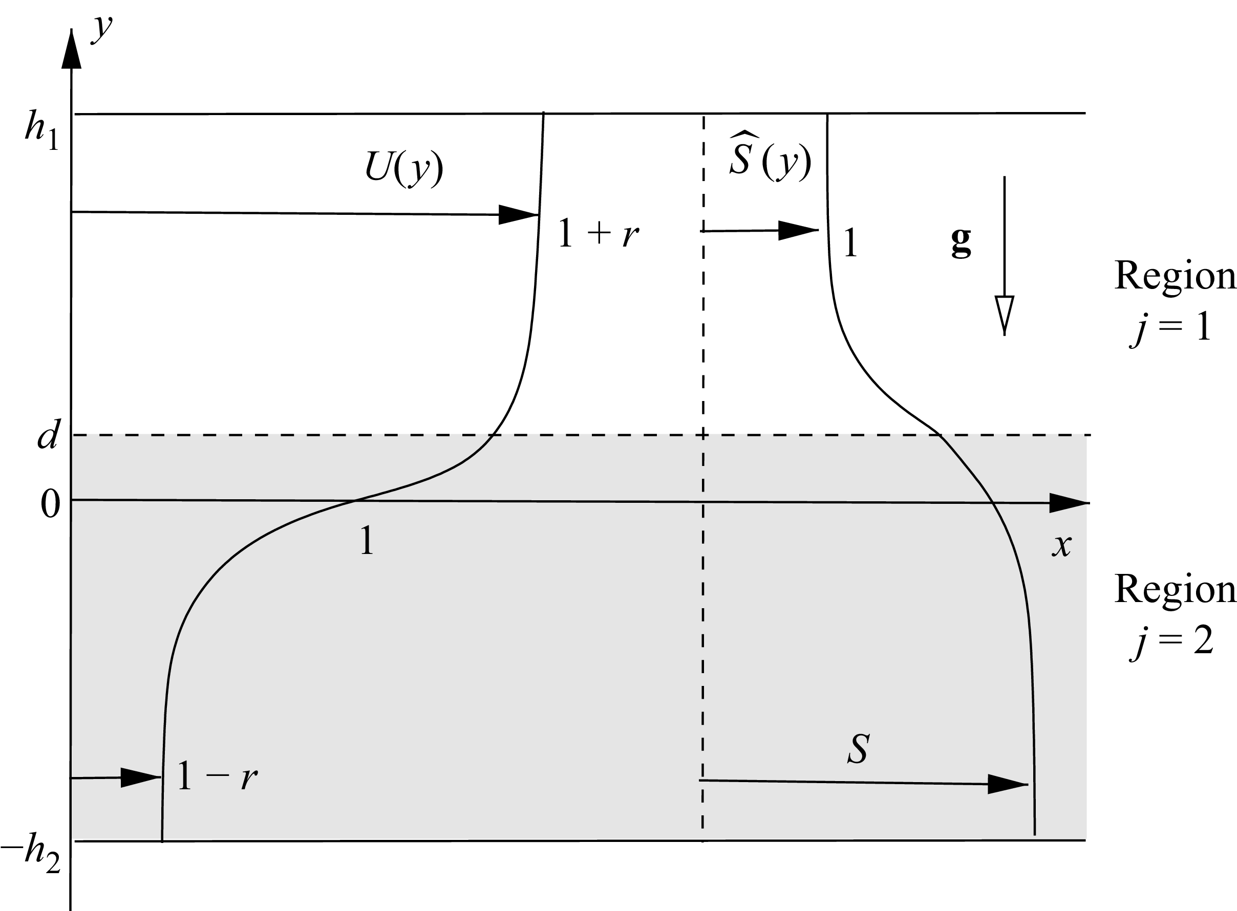


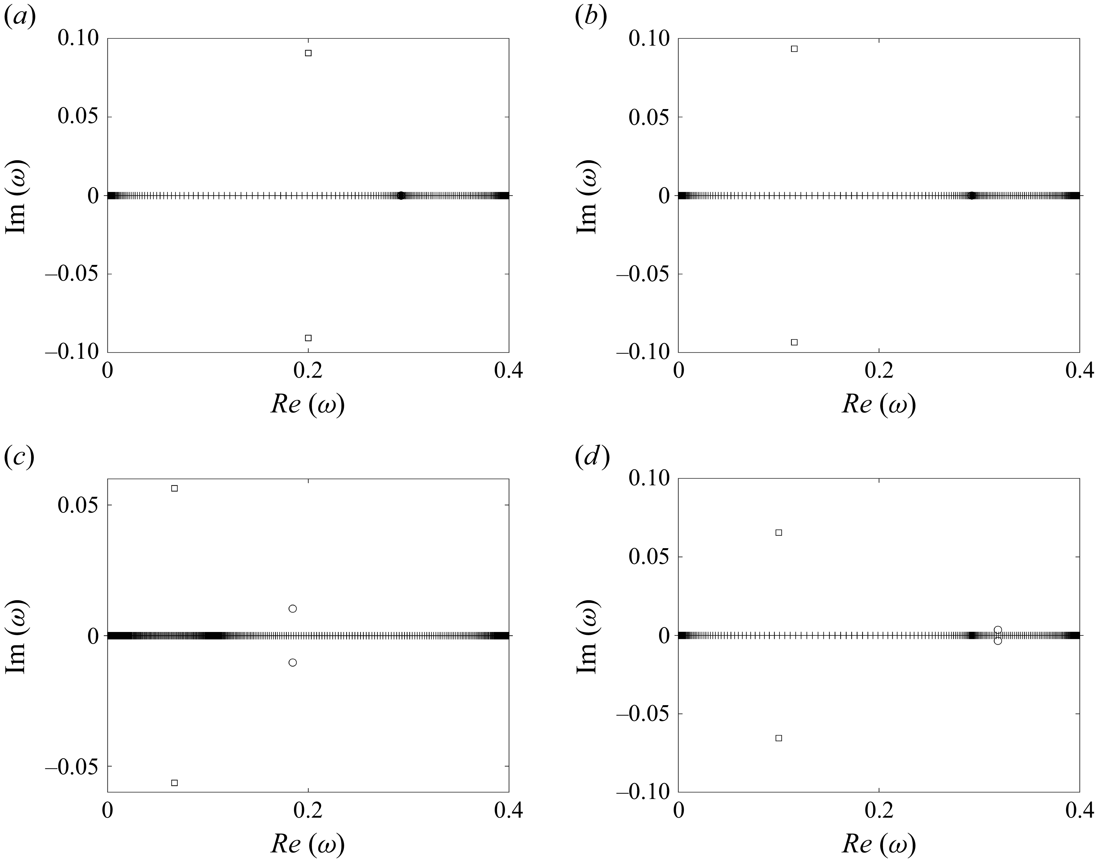


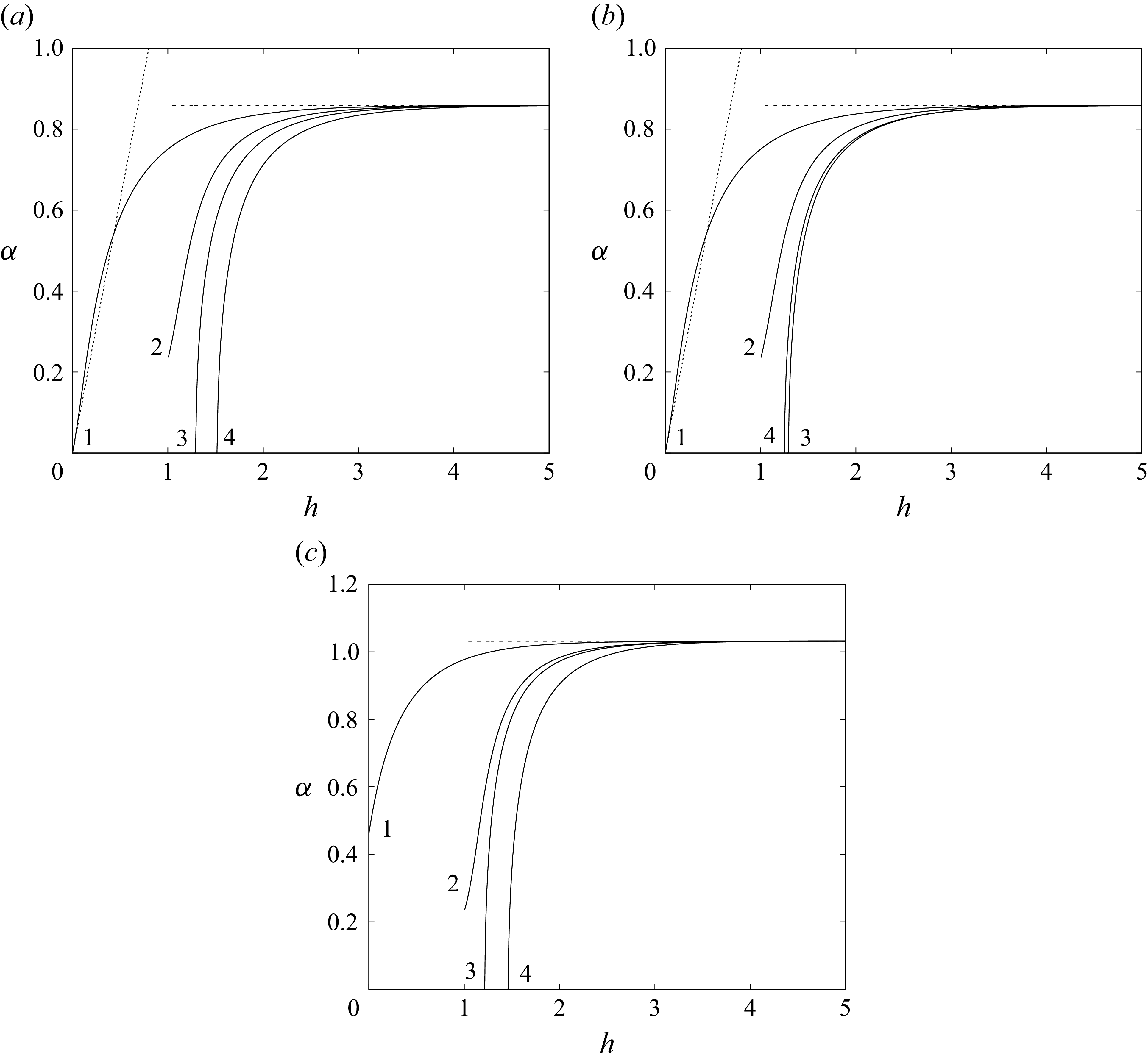


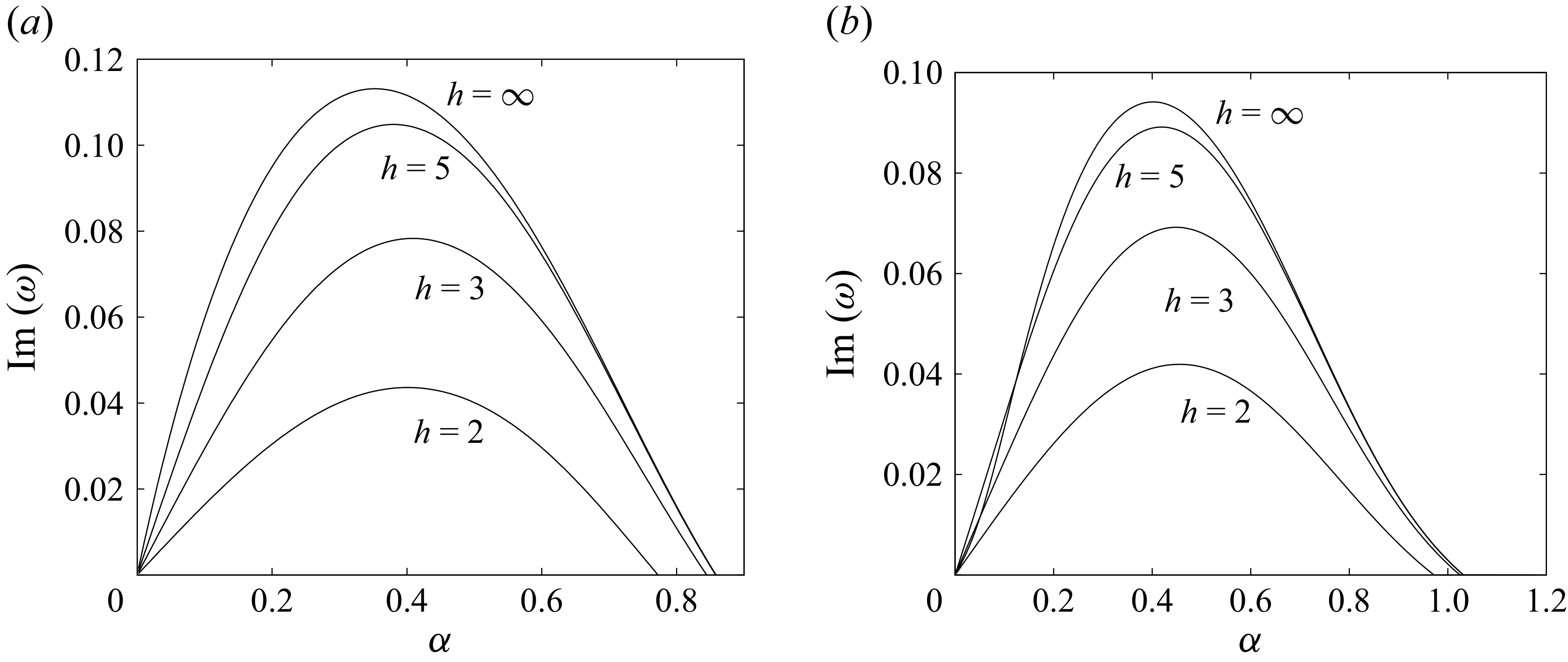


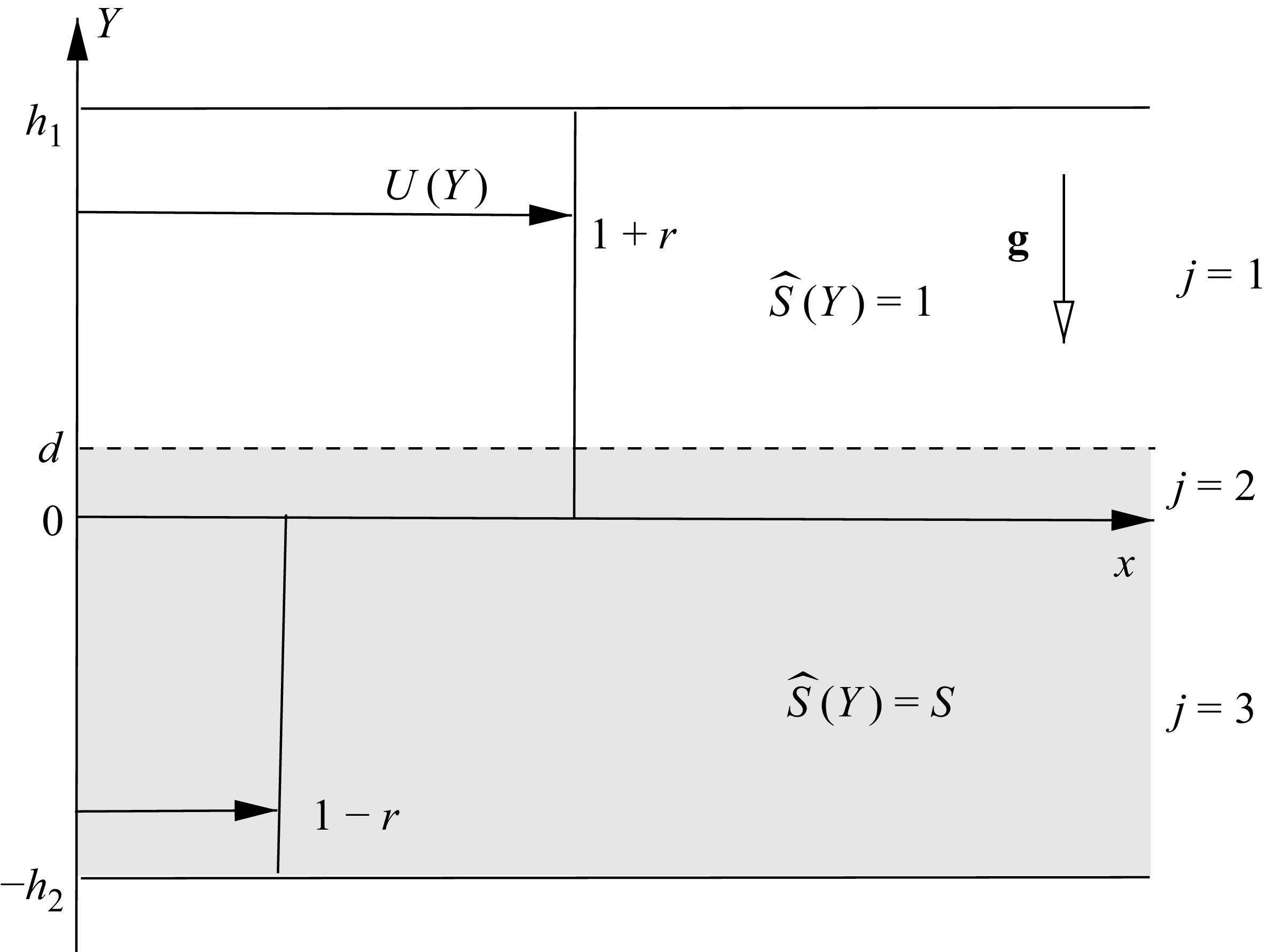


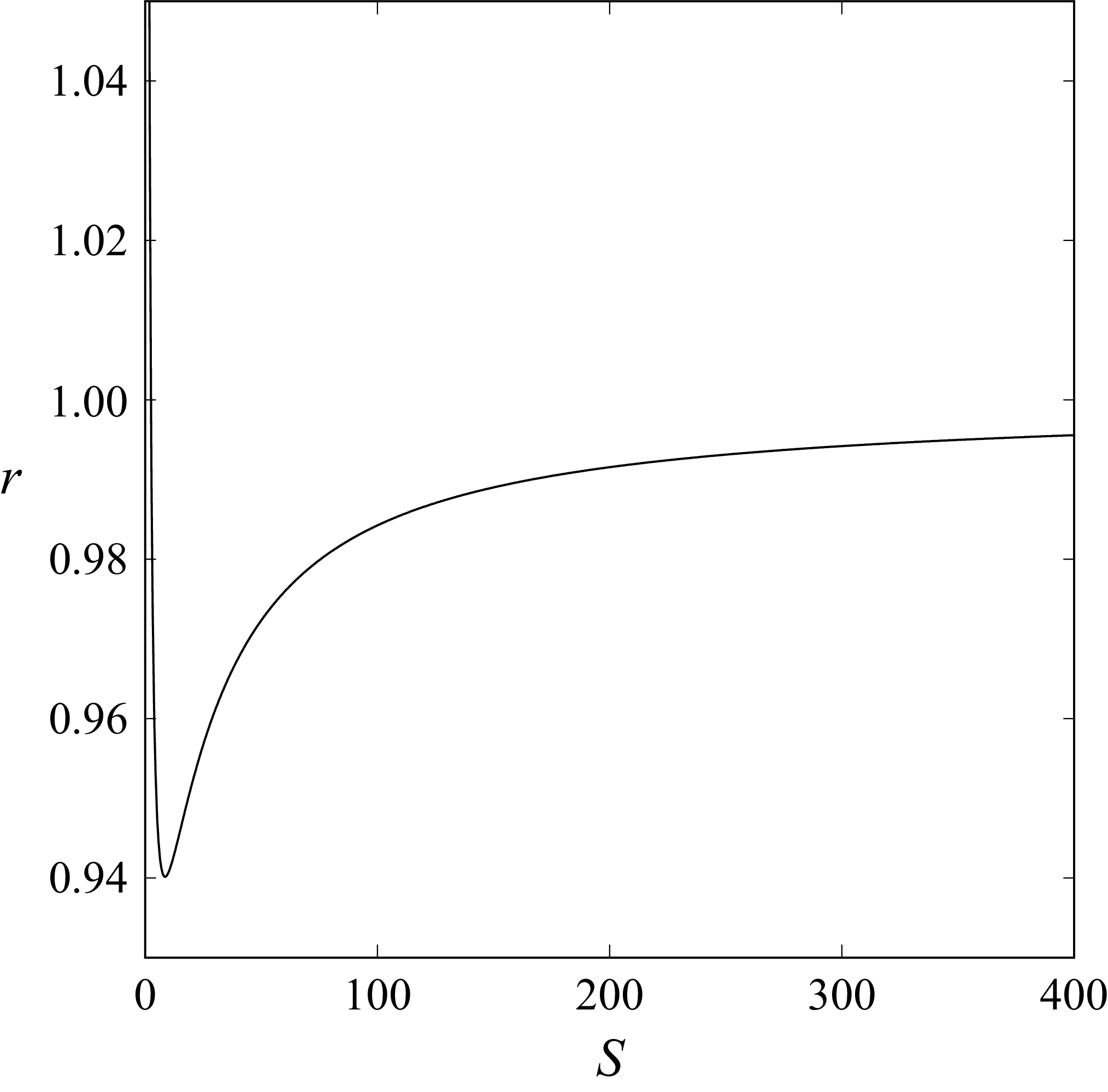


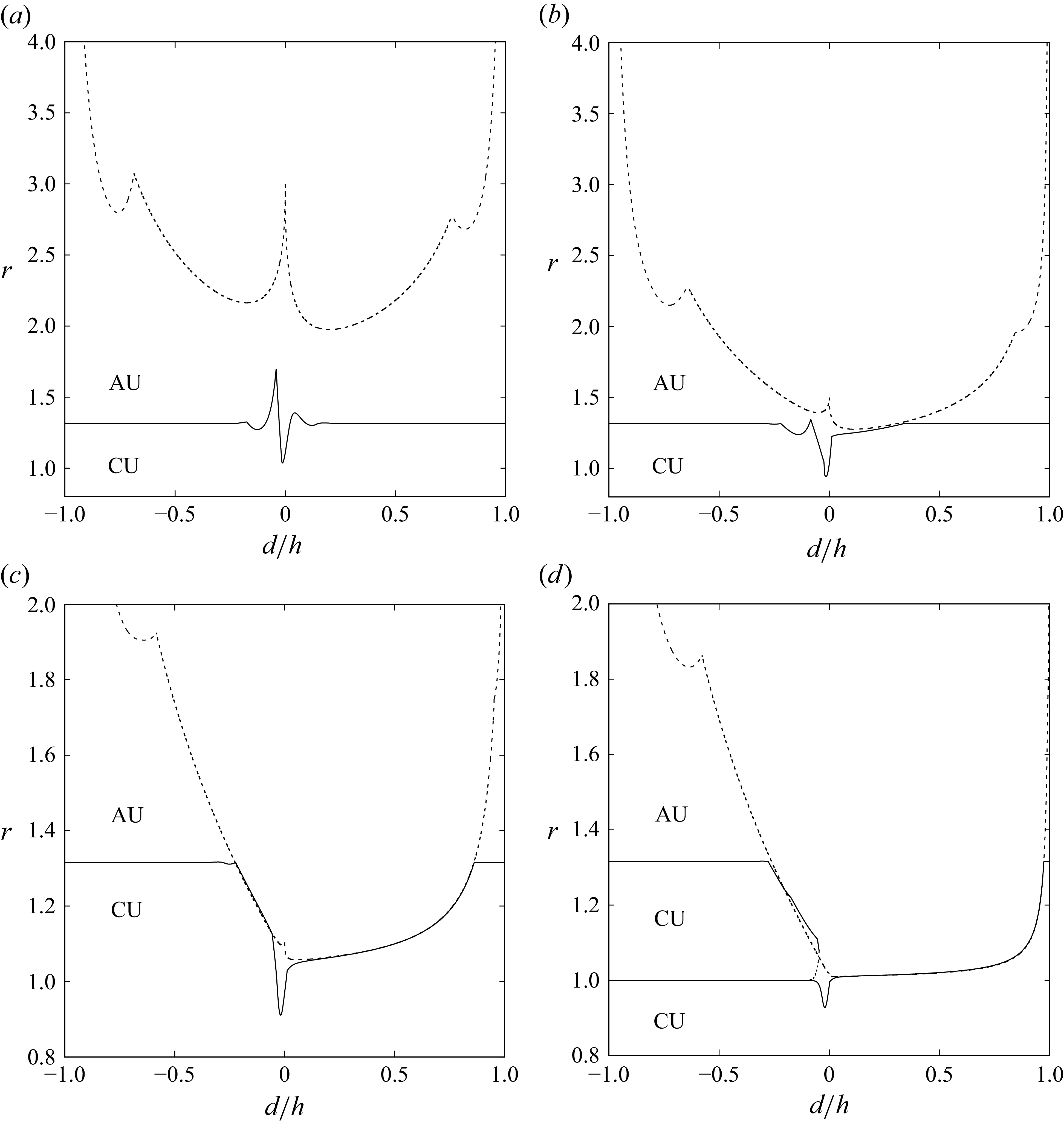


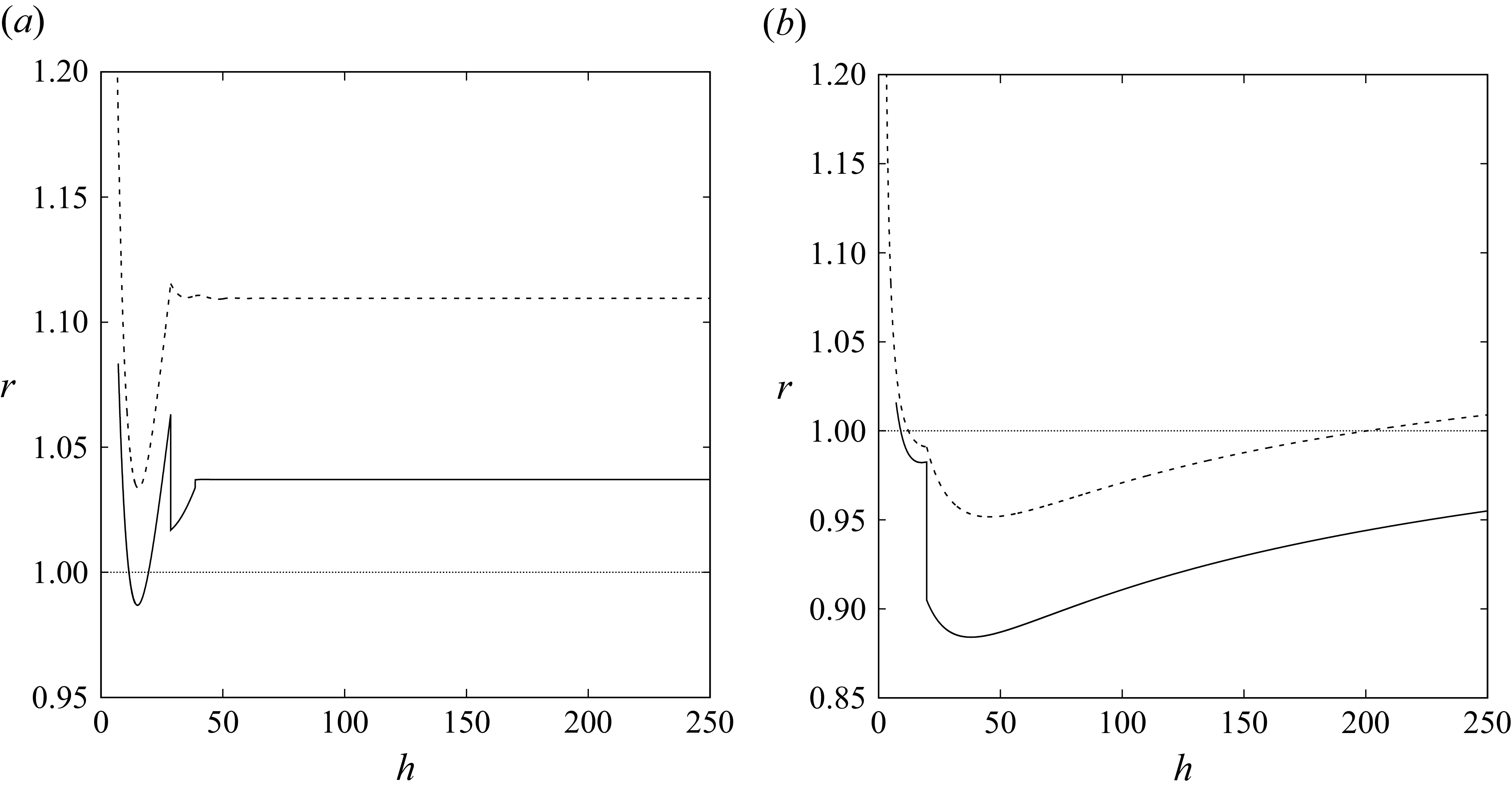


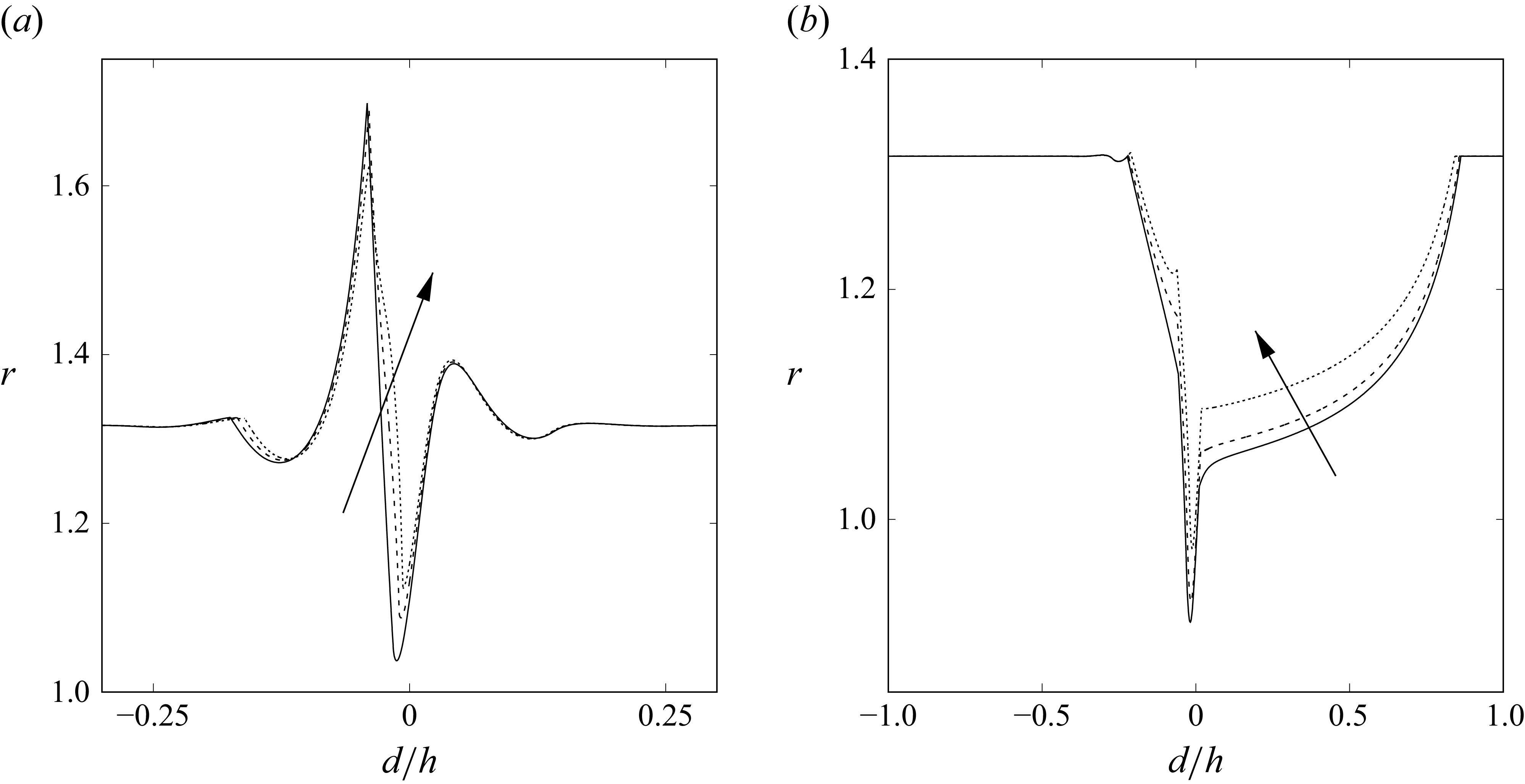


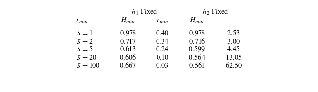


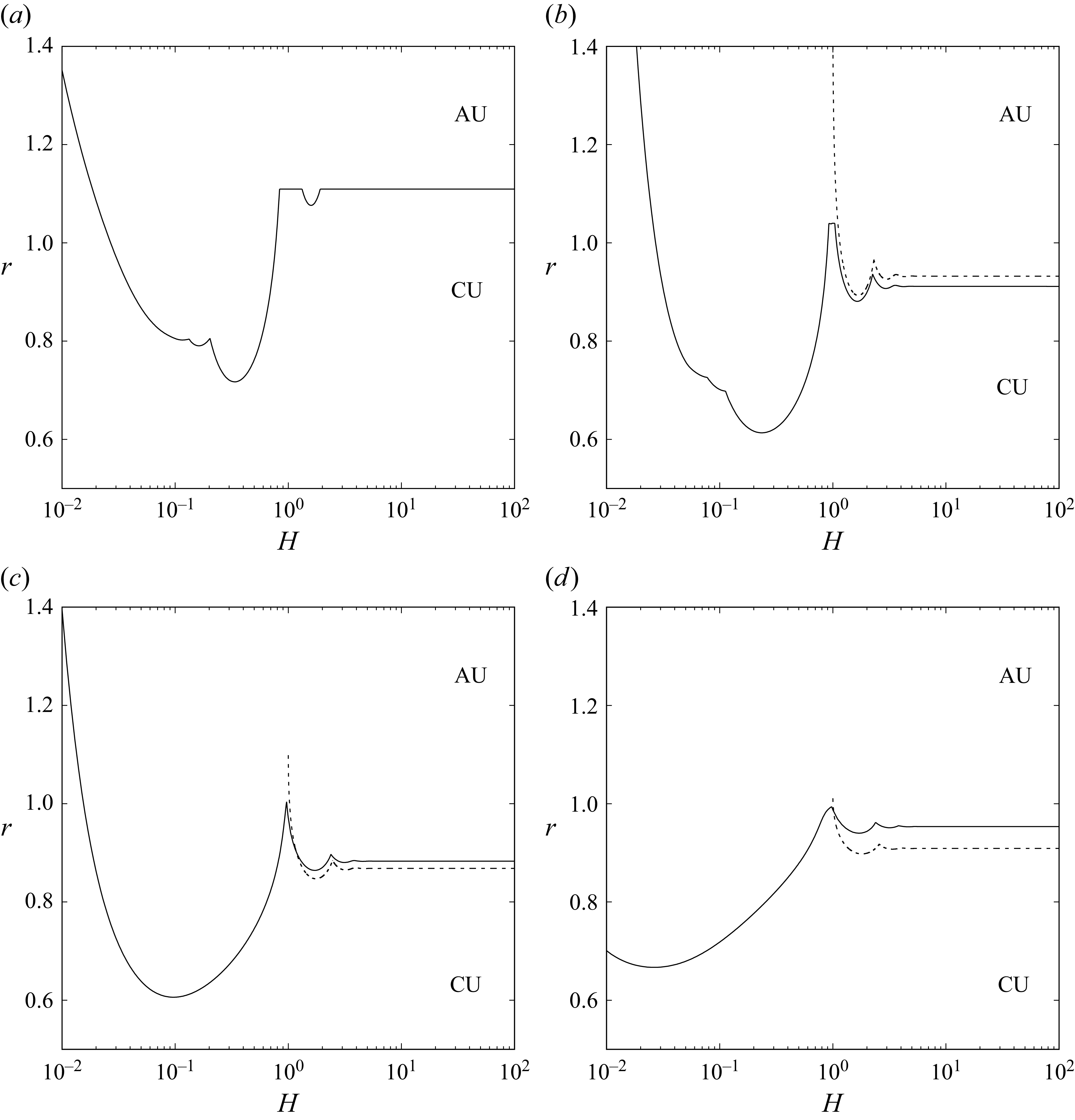


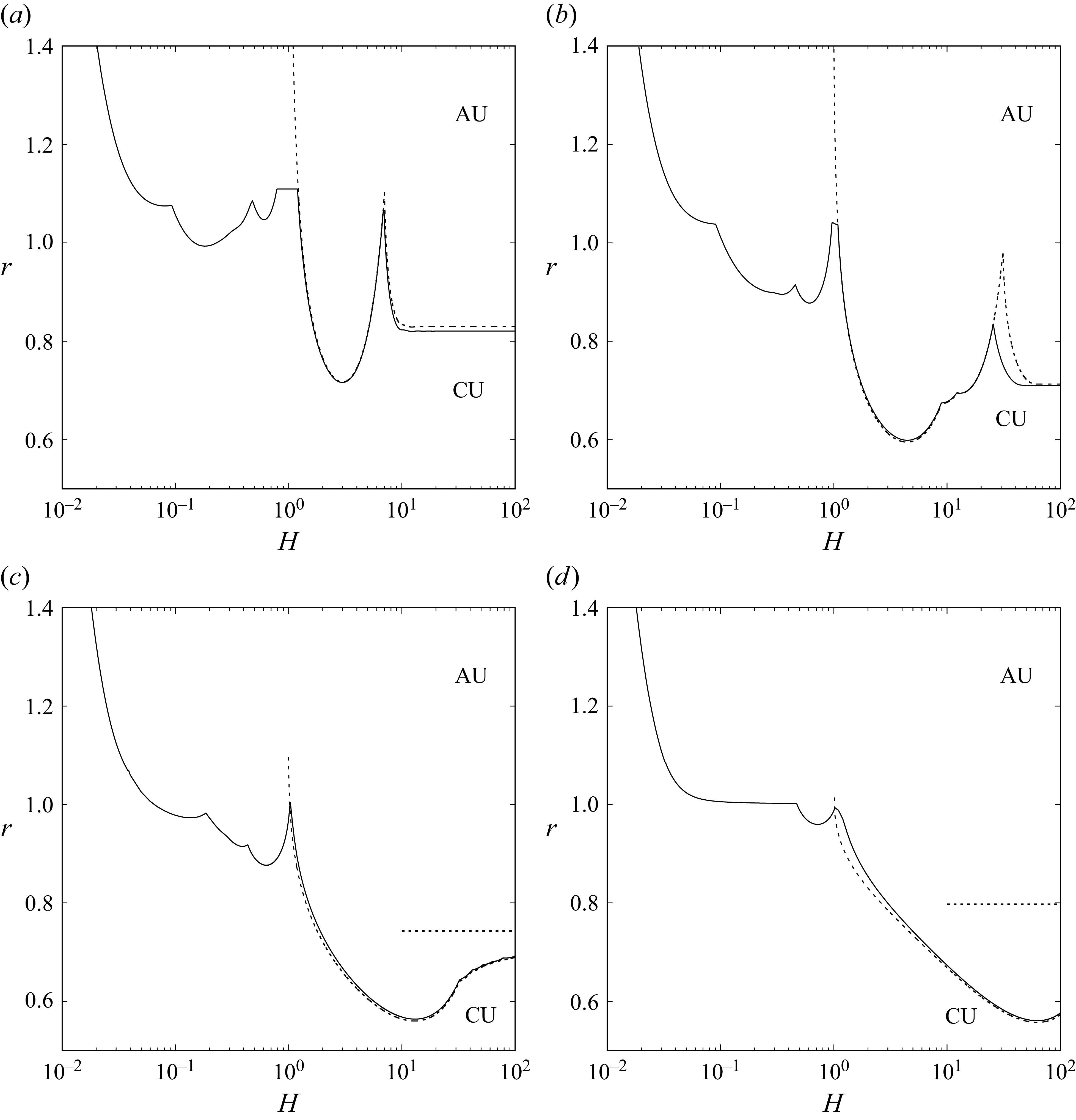


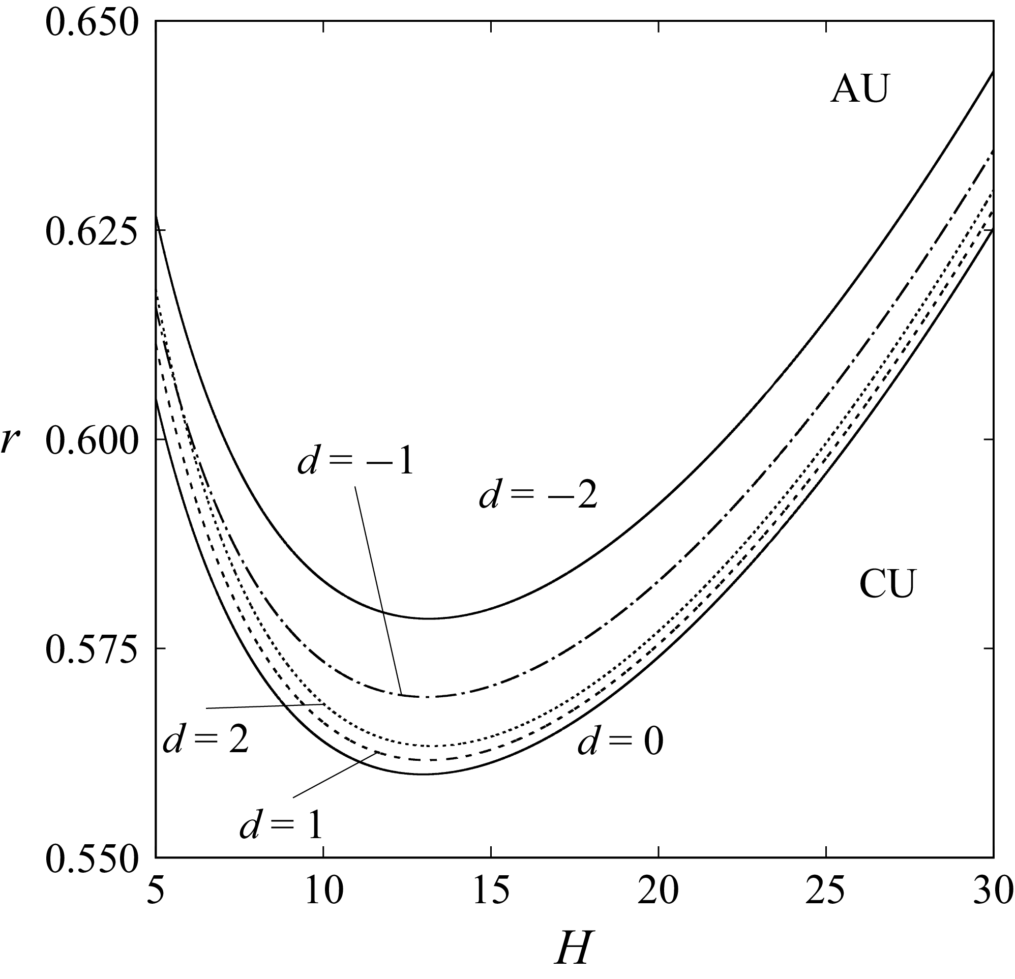


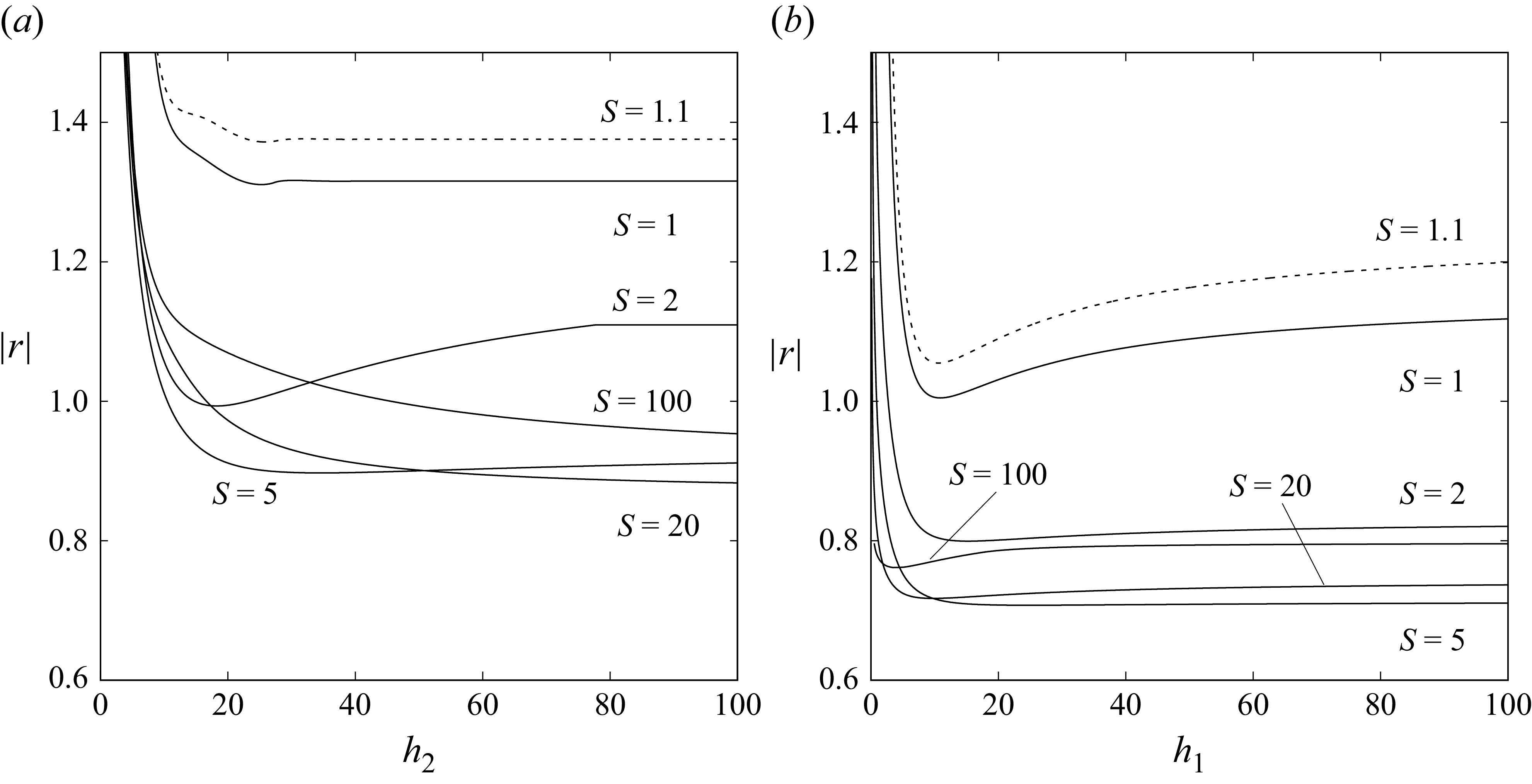


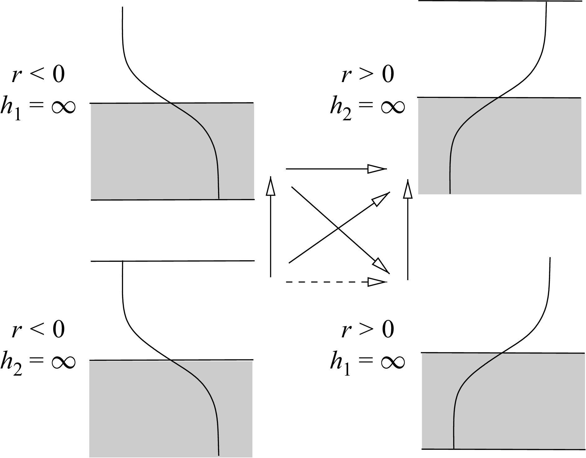

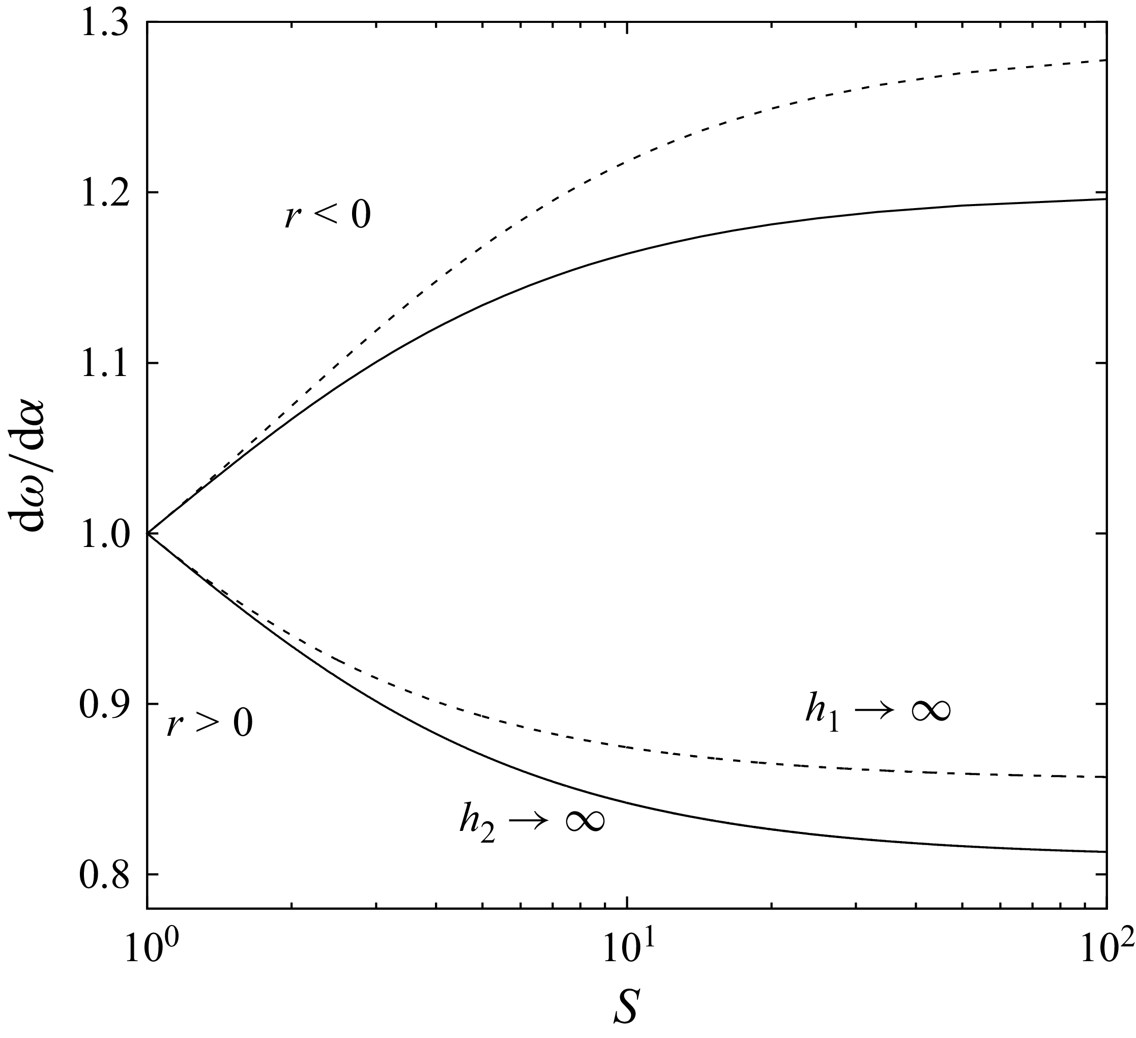


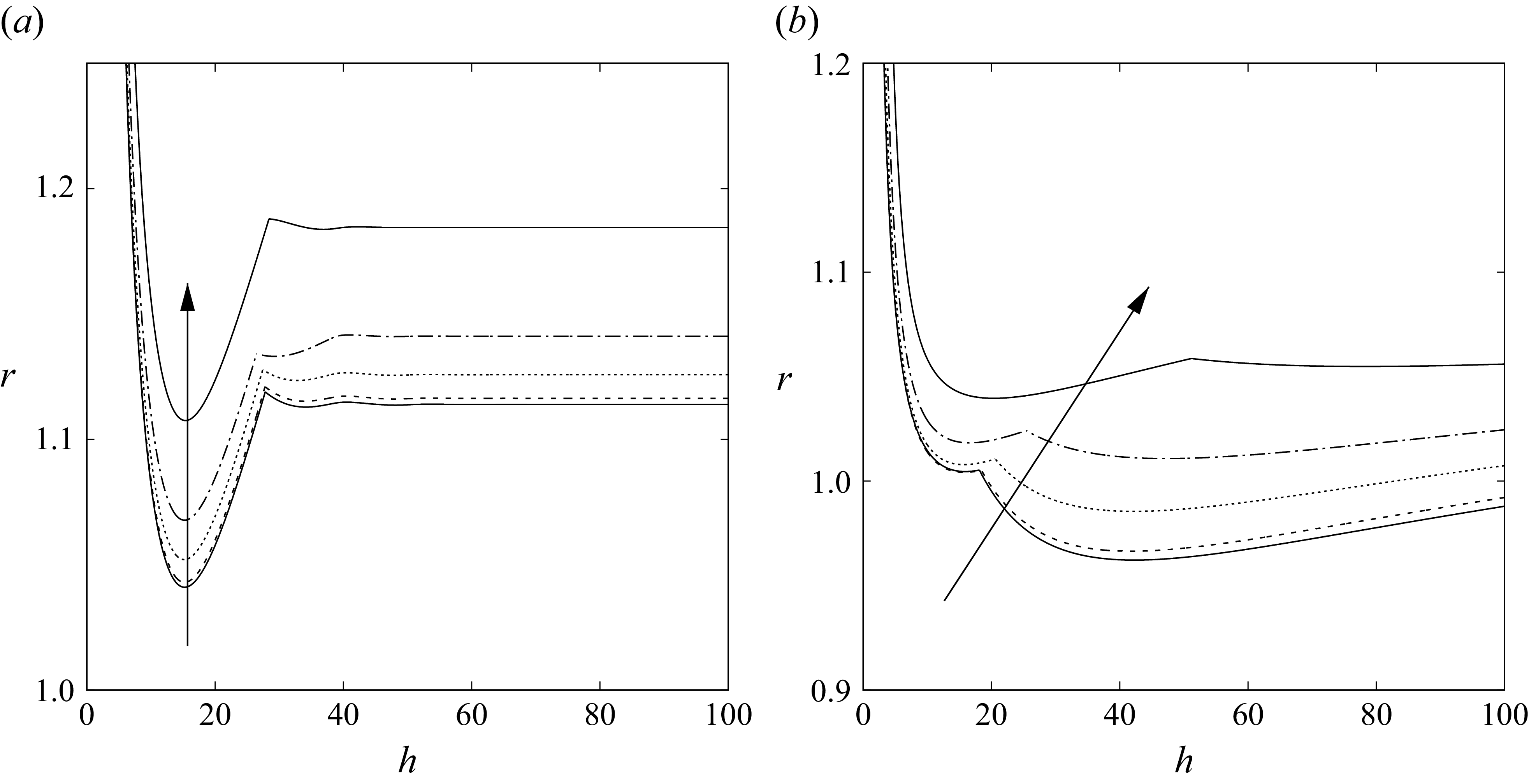


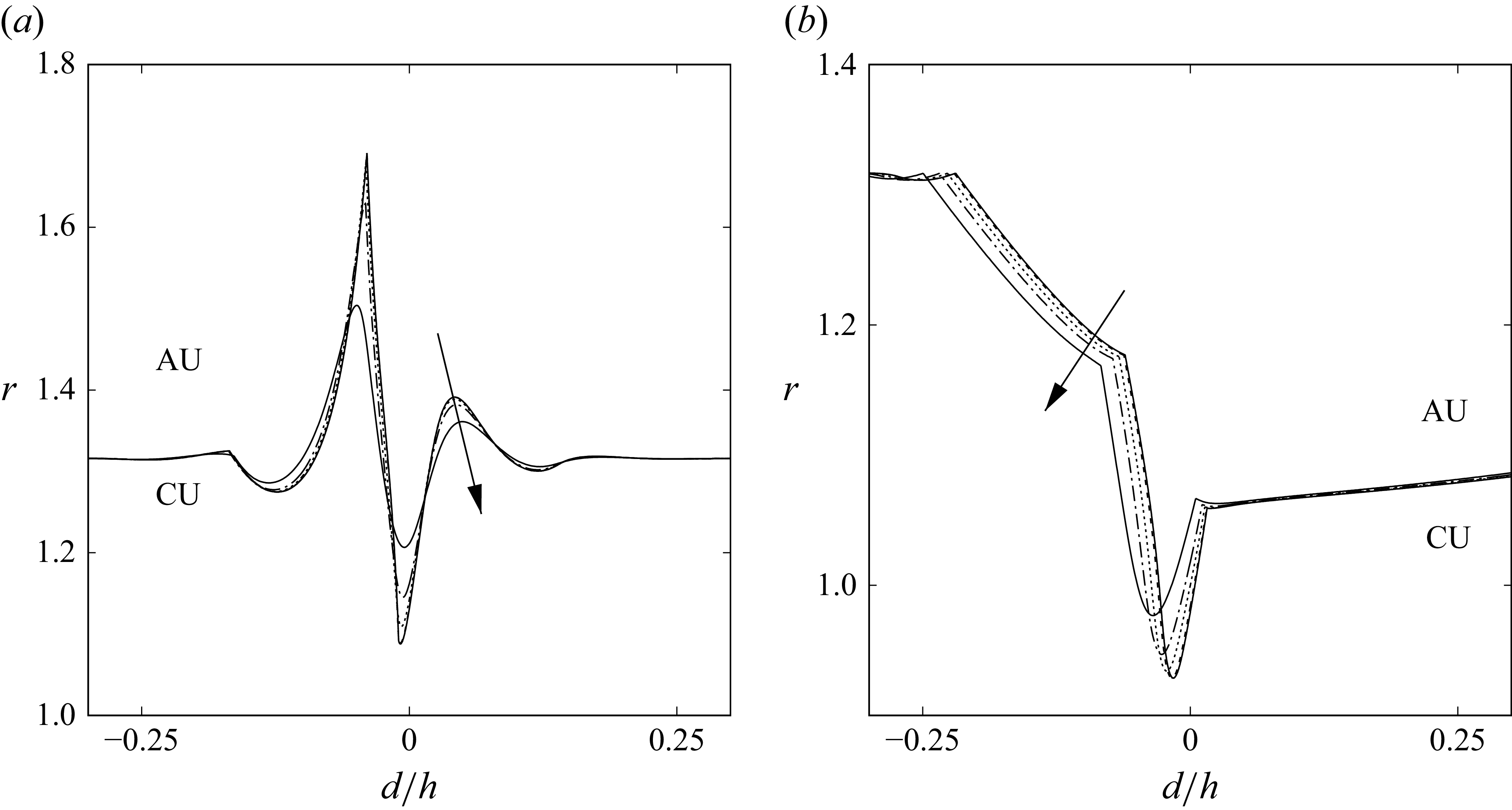


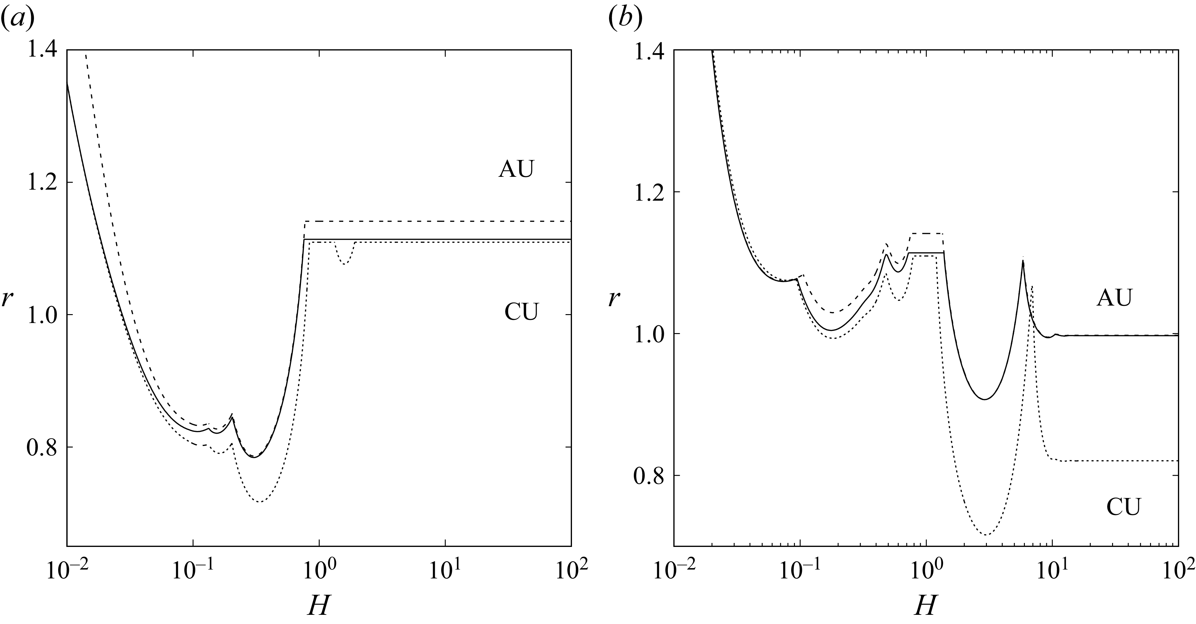


 Open access

