Anthropometry

Searching for a measure of human working efficiency, Jindrich Matiegka reported in 1921 what was to become a classic anthropometric approach to quantifying skeletal muscle mass⁽ Reference Matiegka ^{22 )}. Matiegka's method divided body weight into four parts: skeleton, skeletal muscle, skin plus subcutaneous adipose tissue and remainder. Crude measuring devices were used to quantify bone and extremity breadths and skinfold thickness. Estimated values were then incorporated along with the height and calculated surface area into Matiegka's body composition prediction model. Seven decades later Martin et al. reported in 1990 one of the first whole-body anthropometric skeletal muscle prediction models by post-mortem calibration against twelve male subjects in the Brussels Cadaver Study (Table 2)⁽ Reference Martin, Spenst and Drinkwater ^{23 )}. Doupe et al. reported an updated version of Martin's model in 1997⁽ Reference Doupe, Martin and Searle ^{24 )}.

Table 2.

Some method-specific equations used to estimate regional and total skeletal muscle mass

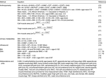
BIA, bioimpedance analysis; DXA, dual-energy X-ray absorptiometry.

Others that followed Matiegka and later Martin were limited by a lack of reference standards for in vivo skeletal muscle mass measurement until the introduction of computed tomography (CT) by Hounsfield⁽ Reference Hounsfield ^{25 )}. Since then CT, MRI and dual-energy X-ray absorptiometry (DXA) have all been used as the reference for developing anthropometric skeletal muscle mass prediction equations. Expanding on the Brussels Cadaver Study strategy, Lee et al.⁽ Reference Lee, Wang and Heymsfield ^{17 )} reported anthropometric skeletal muscle mass prediction equations developed in 244 adults using MRI as the reference (Table 2).

The most recent anthropometric approach was reported in 2014 by Al-Gindan et al.⁽ Reference Al-Gindan, Hankey and Govan ^{26 )} using total body skeletal muscle mass collected on 423 adults varying in age, sex, race and BMI using whole-body MRI as the reference. An additional 197 subjects served as a validation sample. The author's main aim was to develop equations that incorporated commonly used measures that typically are collected in large population studies and surveys. The Al-Gindan prediction equations are summarised for men (derivation: R ² 0·76, standard error of the estimate (see) 2·7 kg; validation: R ² 0·79, see 2·7 kg) and women (derivation: R ² 0·58, see 2·2 kg; validation: R ² 0·59, see 2·1 kg) in Table 2.

Simple regional skeletal muscle estimation approaches are also available that are practical to apply in the clinical setting. For example, appendicular cross-sectional muscle plus bone areas can be derived using a combination of skinfold and circumference measurements (Table 2)⁽ Reference Heymsfield ^{27 ,} Reference Heymsfield, McManus and Smith ^{28 )}. Similar equations are also available that correct for bone inclusion within the skeletal muscle compartment⁽ Reference Heymsfield, McManus and Smith ^{28 )}.

While anthropometry as a means of estimating skeletal muscle mass has several important advantages, use in the elderly poses problems not encountered in younger adults and children. These strengths and limitations of anthropometry are summarised in Table 1. Notably, anthropometric measurements are unable to discern the active contractile components from adipose and connective tissues embedded within the muscle compartment. These components may impact functional measures and account for the often-observed dissociation that occurs over time with ageing between skeletal muscle mass and function⁽ Reference Newman, Kupelian and Visser ^{29 ,} Reference Goodpaster, Park and Harris ^{30 )}.

Urinary markers

Discovered in meat by Chevreul in 1835, creatine is a metabolite distributed primarily in skeletal muscle and to a lesser extent in brain and other tissues⁽ Reference Chevreul ^{31 )}. Creatine undergoes non-enzymatic degradation to creatinine at a stable rate and this metabolic end-product is then excreted unchanged in urine. Urine collected over 24 h from subjects ingesting a meat-free diet can be analysed for creatinine and early workers assumed levels are directly proportional to skeletal muscle mass (1 g = about 20 kg)⁽ Reference Heymsfield, Arteaga and McManus ^{32 )}. Forbes and Bruining in 1976 developed a urinary creatinine prediction equation with total body potassium-measured ‘lean body mass’ as the reference for skeletal muscle (Table 2)⁽ Reference Forbes and Bruining ^{33 )}.

With the introduction of CT in the 1970s it became possible for the first time to accurately quantify the total body skeletal muscle mass in living subjects. Wang et al. in 1996 used CT to quantify the relation between 24 h urinary creatinine and skeletal muscle mass in twelve healthy men (Table 2, R 0·92, see 1·89 kg; P < 0·001)⁽ Reference Wang, Sun and Heymsfield ^{34 )}. More recently, Clark and Manini⁽ Reference Clark and Manini ^{35 )} used MRI to measure skeletal muscle mass in subjects ingesting a gel capsule filled with deuterated creatine (DCR). The stable isotope DCR provides a means of measuring the subject's total body creatine pool size with mass spectroscopy used to analyse urine samples collected over several days. Skeletal muscle mass measured by DCR was well correlated with skeletal muscle mass measured with MRI as the reference (R 0·868, P < 0·001)⁽ Reference Clark and Manini ^{35 )}. A recent study by Patel et al.⁽ Reference Patel, Molnar and Tayek ^{36 )} advanced the concept that serum creatinine can serve as a biomarker of skeletal muscle mass assuming adjustments are made for renal function and dietary meat intake.

Urinary Ntau-methylhistidine (3-methylhistidine) has also been used to estimate skeletal muscle mass⁽ Reference Lukaski, Mendez and Buskirk ^{37 )}. Skeletal muscle contractile proteins, actin and myosin, are methylated after completion of peptide bond synthesis leading to the production of 3-methylhistidine. The 3-methylhistidine is released with protein catabolism and excreted unchanged in the urine. While urinary 3-methylhistidine collected over 24 h is typically used to evaluate the rate of myofibrillar protein breakdown, empirical skeletal muscle mass prediction equations have also been published (Table 2). Because of 3-methylhistidine's complex metabolism, analytical costs and introduction of other competing methods, few workers today continue to use this metabolic end-product as a means of estimating skeletal muscle mass.

A limitation of urinary creatinine and 3-methylhistidine as markers of skeletal muscle mass is the requirement for dietary control and multiple 24-h urine collections that are applied together for optimum results. In the absence of other available methods, however, the cost of these approaches is minimal and there are no subject safety concerns as with some imaging methods. Additional research is needed on the use of DCR and serum creatinine for quantifying skeletal muscle mass.

Separate from measurement concerns, the two urinary markers conceptually reflect muscle cell mass rather than whole muscle that also includes embedded adipose tissue, connective tissues and extracellular fluid. Anthropometry, which measures whole muscle, may therefore give differing impressions of age-related chances than a marker such as urinary creatinine or DCR that capture muscle cell mass.

Ultrasound

Recent technological advances provide new opportunities for application of ultrasound in evaluating skeletal muscle mass and quality. Karl Dussik at the University of Vienna was the first to apply ultrasound methods in 1942 with early attempts at diagnosing brain tumours⁽ Reference Dussik ^{38 )}. Eight years later, George Ludwig at the United States Naval Research Institute further improved ultrasound methods for diagnosing the presence of gallstones⁽ Reference Ludwig, Bolt and Heuter ^{39 )}. A piezoelectric crystal housed in the transducer probe produced high-frequency sound waves. The directed sound waves passed through the skin surface and then reflected off underlying anatomic structures, including skeletal muscle and bone interfaces. Returning sound waves, or echoes, were then captured by a receiver housed in the transducer probe. The same fundamental technology is in use today.

A-mode ultrasound emerged in the 1960s as an alternative to skinfold calipers in evaluating subcutaneous adipose tissue layer thickness⁽ Reference Pillen and van Alfen ^{40 )}. A-mode systems provide an amplitude-modulated display that represents the intensity of returning echoes. This allows visualisation of various tissue interfaces and thereby measurement of fat and muscle ‘thickness’ at pre-defined anatomic sites. Commercial A-mode systems are in use today for measuring adipose tissue and skeletal muscle thickness at pre-defined anatomic sites⁽ Reference Smith-Ryan, Fultz and Melvin ^{41 )}. More recently B-mode systems provide a brightness-modulated display for echoes returning to the system transducer. B-mode systems display two-dimensional cross-sectional images of adipose tissue, skeletal muscle and bone structures. Newer ultrasound systems provide three-dimensional skeletal muscle images and thus selected total muscle volumes⁽ Reference Dietz ^{42 )}.

Two investigators at the University of Tokyo, Ikai and Fukunaga, were among the first to use ultrasound for measuring skeletal muscle cross-sectional areas in 1968⁽ Reference Ikai and Fukunaga ^{43 )}. Sanada et al.⁽ Reference Sanada, Kearns and Midorikawa ^{44 )} measured skeletal muscle thickness in Japanese adults with ultrasound at several anatomic sites and the authors reported total body prediction equations using MRI as the reference. Abe et al.⁽ Reference Abe, Loenneke and Young ^{45 )} recently reviewed previously published regional and total muscle mass ultrasound prediction equations using DXA as the reference criterion. The authors observed good correlations between DXA-derived muscle indices and corresponding ultrasound predictions (R all ≥0·9 and P < 0·001) in men and women with variable between-method significant bias, Sanada's total muscle mass equation (Sanada et al.⁽ Reference Sanada, Kearns and Midorikawa ^{44 )}) being the only one without non-significant bias. In another recent report, Loenneke et al.⁽ Reference Loenneke, Thiebaud and Abe ^{46 )} suggested that skeletal muscle thickness measured at the anterior portion of the thigh can be used to track age-related changes in muscle size.

Ultrasound is increasingly being used to provide estimates of skeletal muscle quality. Ultrasound elastography, is a real-time method of visualising the distribution of skeletal muscle tissue strain and elastic modulus⁽ Reference Drakonaki, Allen and Wilson ^{47 )}. Several ultrasound elastography methods are available that differ in the way tissue stress is applied and the method used to detect and reconstruct the displaced tissue image⁽ Reference Drakonaki, Allen and Wilson ^{47 )}. The most common of these is strain ultrasound elastography in which one approach is to manually apply low-frequency tissue compression with the transducer probe. The resulting axial muscle tissue displacement (i.e. strain) can then be detected and quantified. Ageing and sarcopenia through associated changes in skeletal muscle quality (e.g. fibrosis) may result in biomechanical alterations (stiffness and loss of elasticity) that are detectable by ultrasound elastography.

Healthy muscle is echolucent or ‘dark’ as sound waves pass through the homogenous tissue and are reflected back only when they interact with fibrous structures such as vasculature and epimysium⁽ Reference Harris-Love, Monfaredi and Ismail ^{48 )}. As subjects age and develop sarcopenia skeletal muscles increasingly have adipose tissue infiltration and fibrosis that lead to new sound reflection planes⁽ Reference Pedersen, Fredberg and Langberg ^{49 )}. These changes are accompanied by an increase in echogenicity, indicated as whiter muscles in ultrasonography, and the amount of ‘white’ and ‘dark’ muscle tissue of the sonographic images can be quantified by the degree of the echolucencies in human subjects⁽ Reference Pillen and van Alfen ^{40 ,} Reference Watanabe, Yamada and Fukumoto ^{50 )}. These effects are readily evaluated using ultrasound imaging software. As a representative example, Watanabe et al.⁽ Reference Watanabe, Yamada and Fukumoto ^{50 )} recently observed an inverse association between echo intensity and muscle strength in elderly men.

Bioimpedance analysis

Bioimpedance analysis (BIA) was pioneered in the 1950s and 1960s by Hoffer, Nyboer and Thomasset⁽ Reference Hoffer, Meador and Simpson ^{51 –} Reference Thomasset ^{53 )}. Today BIA is widely used in the study of human body composition as instruments are available, relatively inexpensive and analyses require minimal technician participation even when using research-grade systems. When a weak alternating current is applied across a limb the net conductivity reflects features of the traversed tissues⁽ Reference Hoffer, Meador and Simpson ^{51 )}. Fluid and electrolyte-rich soft tissues, particularly skeletal muscle, are highly conductive by comparison with low-hydration tissues such as bone. All BIA systems exploit these tissue-specific conductivity differences to quantify body compartments such as skeletal muscle and adipose tissue.

Many system designs are available that range from single to multiple frequency, employ contact or gel-electrodes and that measure segmental or whole-body electrical pathways. All BIA systems measure impedance and/or its two components, resistance and reactance. These electrical measurements in turn can be incorporated into body composition prediction models that have empirical and/or theoretical underpinnings.

The most important advance in relation to skeletal muscle was reported by Organ et al.⁽ Reference Organ, Bradham and Gore ^{54 )}. Organ et al. first described a six-electrode method for segmental BIA that allowed isolation of separate electrical properties of each extremity and the trunk. Several years later Tan et al.⁽ Reference Tan, Birdsell and Martin ^{55 )} described construction of an eight-electrode BIA stand that included contact electrodes for the upright subject's feet and hands. The impedance measures of the arm and leg could then be empirically calibrated to either DXA appendicular lean soft tissue mass (ALST), mainly skeletal muscle or MRI-derived skeletal muscle mass.

Brown et al.⁽ Reference Brown, Karatzas and Nakielny ^{56 )} were the first to use BIA for estimating upper arm cross-sectional muscle and fat areas using CT as the reference. By 2000 Janssen et al.⁽ Reference Janssen, Heymsfield and Wang ^{9 )} reported a whole-body skeletal muscle mass BIA prediction equation using MRI as the calibration method (Table 2). Today several commercially available BIA systems report appendicular and even whole-body skeletal muscle mass with DXA as the usual reference for extremity estimates. We recently reported good correlations between BIA-derived (MC-980, Tanita Corp., Tokyo, Japan) appendicular skeletal muscle mass and corresponding DXA (iDXA, GE Lunar, Madison, WI, USA) lean soft tissue estimates (R ² 0·92, P < 0·001) in 130 children and adults⁽ Reference Jolene Zheng, Gao and Watson ^{57 )}. Most commercial BIA systems rely on proprietary prediction equations for total and regional fat and skeletal muscle mass.

In addition to skeletal muscle estimates, BIA also can provide measures of muscle quality and function. Phase angle can be assessed directly from the relationship between the measured resistance (R) and reactance (Xc) values (Phase angle (°) = arctangent (Xc/R) × (180/π)). Phase angle not only provides useful body composition information, but also reflects cell membrane function and it has clinical prognostic value⁽ Reference Norman, Stobaus and Pirlich ^{58 )}. Although the underlying biological mechanisms of phase angle are not well defined, a recent study⁽ Reference Norman, Stobaus and Pirlich ^{58 )} suggests that age is a main determinant after controlling for other covariates. Data from several large-scale studies across different countries and race/ethnic groups show a consistent pattern with peak phase angle values during early adulthood and then values gradually decline in later years independent of body composition⁽ Reference Norman, Stobaus and Pirlich ^{58 )}. The basis of this age-related decline in phase angle is not well understood but parallel changes are observed in skeletal muscle ultrasound echogenicity⁽ Reference Fukumoto, Ikezoe and Yamada ^{59 )}, a finding suggesting that chemical and anatomic changes in muscle may account in part for the observed effects. In a recent study, Basile et al.⁽ Reference Basile, Della-Morte and Cacciatore ^{60 )} reported independent effects of grip strength and skeletal muscle mass on phase angle measured in a cohort of elderly adults; low phase angle was associated with reduced grip strength. Slee et al.⁽ Reference Slee, Birch and Stokoe ^{61 )} evaluated a cohort of frail older hospitalised patients, some of whom were malnourished, and observed a low phase angle compared with healthy elderly reference values⁽ Reference Slee, Birch and Stokoe ^{61 )}. Age-related changes in other BIA resistance and reactance ratios and combinations at different frequencies are also recognised. Taken together these findings suggest that BIA may provide information on skeletal muscle quality that may ultimately yield prognostic information.

Body weight scales that incorporate BIA technology through contact foot electrodes can also be modified to provide functional and balance information⁽ Reference Sun ^{62 )}. The scale platform force transducers can capture the subject's generated power and stability as they stand erect from a stable crouched or seating position. With appropriate protocols these kinds of instruments, now in development, can potentially yield information on skeletal muscle mass, composition (e.g. phase angle or other age-related BIA measure) and functionality.

The strengths and limitations of BIA are summarised in Table 1. Since so many systems differing in design are available, generalisations on accuracy and overall quality are not possible in the context of this review. The features and supporting literature for each instrument should be scrutinised by the interested investigator or clinician. Of importance for all BIA systems is the presence of stable subject conditions at the time of measurement. Hydration, time of day and many other factors influence measured subject impedance values and meticulous adherence to manufacturer-specified conditions will ensure optimum results.

Imaging

The discovery of X-rays by Röentgen in 1895 transformed not only clinical medicine, but the field of body composition research as a whole. By 1942 Harold C. Stuart and P. Hill-Dwinell at Harvard evaluated muscle and fat ‘widths’ in growing children⁽ Reference Stuart and Hill-Dwinell ^{63 )}. Godfrey Hounsfield at EMI in London revolutionised biomedical imaging with the introduction of the first functional CT scanner in 1975⁽ Reference Wells ^{64 )} and not long after three publications on CT-measured skeletal muscle appeared between 1978 and 1979⁽ Reference Bulcke, Termote and Palmers ^{65 –} Reference Heymsfield, Olafson and Kutner ^{67 )}. CT provided the first accurate approach for quantifying whole-body muscle mass in living human subjects in the mid-1980s⁽ Reference Tokunaga, Matsuzawa and Ishikawa ^{68 ,} Reference Sjöström ^{69 )}.

Following up on a long series of important discoveries in physics, Raymond Damadian at SUNY Downstate introduced the first human MRI scanner in 1977⁽ Reference Macchia, Termine and Buchen ^{70 )}. Studies of skeletal muscle biology proliferated in the 1980s as MRI system availability increased and investigators were able to scan subjects of all ages without the radiation concerns associated with CT. Working with a skeletal orientation related to osteoporosis, Mazess et al. first introduced the dual-photon absorptiometry concept in 1970 for bone evaluation in the presence of overlying soft tissues⁽ Reference Mazess, Cameron and Sorenson ^{71 )}. Modern DXA systems that can also provide body composition estimates, including measures of skeletal muscle mass, were introduced in the late 1980s⁽ Reference Kelly, Slovik and Schoenfeld ^{72 )}. Thus, within several decades the body composition field went from relying on such limited skeletal muscle mass estimation methods as anthropometry and urinary creatinine excretion to advanced imaging methods such as CT, MRI and DXA. So far, ten Nobel Prizes have been awarded for development of imaging technology (Supplementary Table S1) that has had a major impact on sarcopenia research and clinical practice.

Computed tomography

CT was the first method introduced that could quantify whole-body and regional skeletal muscle mass with high accuracy. High-resolution cross-sectional images of pre-defined slice width can be analysed for each tissue, including skeletal muscle, using hand segmentation or automated software. Depending on the study, varying numbers of cross-sectional images can be combined to evaluate single muscle areas, volumes or whole-body skeletal muscle mass.

Each image picture element, or pixel, is defined by a linear attenuation coefficient or CT# reported in Hounsfield units (HU). Water is internationally defined as 0 HU and air as −1000 HU. Adipose tissue has negative HU values, whereas skeletal muscle has positive HU values and these tissue X-ray attenuation differences can be exploited for analytical purposes during hand segmentation or by automated software.

The segmented CT scan provides measures of skeletal muscle area and multiple images at specified intervals can be used to derive regional or total volumes. Most investigators then calculate skeletal muscle mass from the measured volume as the product of volume and density, usually assumed as 1·04 g/cm³⁽ Reference Gallagher, Ruts and Visser ^{11 )}.

With ageing, disuse or in pathological states increasing amounts of adipose tissue can be found within skeletal muscles, particularly of the lower extremities⁽ Reference Gallagher, Kuznia and Heshka ^{73 )}. This intermuscular adipose tissue (IMAT) can be quantified during the analysis and the analyst can then report the values for IMAT and IMAT-free skeletal muscle⁽ Reference Addison, Marcus and Lastayo ^{74 )}. At the molecular level, skeletal muscle is composed of proteins, water, electrolytes, lipids and small amounts of other compounds. Each of these molecular species has a known physical density and closely related attenuation and HU in the context of CT. Iron or fat infiltration of the liver raises and lowers hepatic HU values, respectively⁽ Reference Heymsfield and Noel ^{75 )}. These tissue attenuation effects can be exploited to quantify pathological changes within liver and other tissues. Similarly, a low tissue HU may be a marker of lipid or fluid infiltration in skeletal muscles that can be accompanied by functional changes⁽ Reference Goodpaster, Thaete and Simoneau ^{76 )}. CT can thus provide through evaluated HU values a measure of skeletal muscle quality.

An advantage of CT is high-quality image reconstruction and stable attenuation values that aid in image segmentation and also provide a measure of tissue composition and quality. The radiation exposure of CT and relatively high-cost limit current applications mainly to research or in clinical settings that include CT scanning as part of routine patient care⁽ Reference Prado, Maia and Ormsbee ^{77 )}.

Differential absorptiometry

The availability of DXA systems, modest scan cost, low radiation exposure, short scan time and extensive information provided from each scan makes this approach the most widely used in sarcopenia research and clinical practice at the current time. The DXA approach provides estimates of three body compartments, lean soft tissue, bone mineral content and fat for the whole body and at least four regions, head, trunk, arms and legs. DXA also gives additional skeletal information of value in managing osteoporosis and other clinical conditions related to bone biology.

The lean soft tissue found in the arms and legs, referred to as ALST, has a high muscle content that constitutes a large fraction of total body skeletal muscle mass⁽ Reference Heymsfield, Smith and Aulet ^{78 )}. Measured ALST can thus be used as a surrogate measure of skeletal muscle mass and can be calibrated against whole-body values derived by CT or MRI⁽ Reference Kim, Wang and Heymsfield ^{79 )}. The calibration process provides various prediction equations that can be used to derive total body skeletal muscle mass from the measured ALST value (Table 2).

Since DXA provides measures of regional and total body fat and bone, these components can also be used to evaluate the composite musculoskeletal system (i.e. muscle plus bone) and the level of adiposity. The pathological outcomes associated with sarcopenia often derive from combinations of the amount and quality of skeletal muscle, bone and fat present⁽ Reference Cruz-Jentoft, Baeyens and Bauer ^{80 ,} Reference Stenholm, Harris and Rantanen ^{81 )}.

Magnetic resonance

The introduction of MRI in the 1980s expanded the initial use of CT as means of developing three-dimensional images of skeletal muscle, adipose tissue and other organs. This development is usually referred to as structural or anatomic imaging. The lack of subject exposure to ionising radiation positions MRI as the method of choice for quantifying skeletal muscle across the full lifespan. Most modern MRI scanners can accommodate obese subjects, particularly with the newer wide bore (70 cm) systems.

Water–fat imaging

As with CT, the traditional analysis approach is hand- or partially automated image segmentation. The hand-segmentation approach to the whole-body MRI analysis is tedious, time-consuming and costly. Recent advances in water–fat imaging may soon allow automation of the segmentation process. Relaxation times and resonance frequencies are different for water and fat protons in their respective environments and these differences can be used to suppress the fat-bound signal⁽ Reference Bley, Wieben and Francois ^{82 )}. Two imaging approaches are available for exploiting these differences, relaxation-dependent or short inversion-time recovery and chemical shift-dependent or Dixon-based fat suppression⁽ Reference Bley, Wieben and Francois ^{82 )}. Karlsson et al. recently reported development of a two-point Dixon sequence automated water–fat segmentation method for evaluating total body and regional skeletal muscle volume⁽ Reference Karlsson, Rosander and Romu ^{83 )}. The authors showed excellent test–retest reliability (intraclass correlation coefficient 1·0, 95 % agreement level −0·32 to 0·2 litres) and agreement with hand-segmented images of the lower leg (correlation R values 0·94–0·96) in a follow-up study using a 3T wide-bore MRI scanner and integrated quadrature body coil⁽ Reference Thomas, Newman and Leinhard ^{84 )}. Scan times were about 10 min and the results were evaluated for total body and eight regional skeletal muscle volumes. Shortening the whole-body analysis time is an important advance that could provide an opportunity for evaluating large and diverse samples for prediction model development expanding on the examples presented in Table 2.

In addition to total body and regional skeletal muscle mass, other features of skeletal muscle quality can also be evaluated with MRI and CT such as IMAT⁽ Reference Addison, Marcus and Lastayo ^{74 )}. Skeletal muscle in persons with sarcopenia is characterised by an enlarged IMAT component, notably in the lower extremities⁽ Reference Gallagher, Kuznia and Heshka ^{73 ,} Reference Addison, Marcus and Lastayo ^{74 )}. Water–fat imaging has also been used to evaluate regional skeletal muscle fat infiltration, and as noted earlier, the CT# gives an indication of water and fat infiltration into skeletal muscles⁽ Reference Goodpaster, Thaete and Simoneau ^{76 )}.

An important advance in the context of sarcopenia is a wide array of new magnetic resonance sequences and technology that have the potential to give new structural and functional information about individual muscles and whole-body skeletal muscle mass. These approaches are summarised in Table 3.

Table 3.

Magnetic resonance measurements and approaches for evaluating skeletal muscle that go beyond conventional volumetric rendering

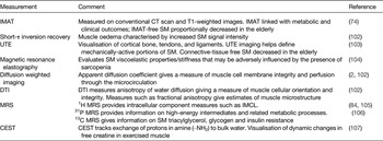
IMAT, intermuscular adipose tissue; CT, computed tomography; UTE, ultra-short echo-time imaging; IMCL, intramyocellular lipid; SM, skeletal muscle; DTI, diffusion tensor imaging; MRS, magnetic resonance spectroscopy; CEST, chemical exchange saturation transfer.

Adjusting measurements for body size

The adult skeletal muscle compartment increases in size as a function of subject stature and adiposity. Quetelet in 1842 first showed that among adults body weight (W) increases as height (Ht) squared (W∝Ht²)⁽ Reference Quetelet, Knox, Smibert and Smibert ^{85 )}. For most populations W/Ht² is independent of height and this observation forms a main basis of BMI⁽ Reference Heymsfield, Peterson and Thomas ^{3 )}. Van Itallie et al. in 1990 suggested that BMI be further divided into two height-normalised indices, fat mass index (FM/Ht²) and fat-free mass index (FFM/Ht²)⁽ Reference Van Itallie, Yang and Heymsfield ^{86 )}. Support for this suggestion came later when Heymsfield et al. showed that adult fat-free mass also scales to height with powers of approximately 2⁽ Reference Heymsfield, Peterson and Thomas ^{3 )}, thus making fat-free mass index independent of height. Baumgartner et al. working with ALST measured with dual-photon absorptiometry, extended Van Itallie's concept by deriving ALST/Ht² as a sarcopenia index ⁽ Reference Baumgartner, Koehler and Gallagher ^{87 )}. Although it now appears as if adult skeletal muscle scales to height with powers slightly greater than 2⁽ Reference Schuna, Peterson and Thomas ^{88 )}, indices such as Baumgartner's would likely only show weak correlations with height.

The growing interest in sarcopenia has led others to suggest additional indices. One explored in the recent Foundation for the National Institutes of Health sarcopenia guidelines is appendicular lean mass (i.e. ALST)/BMI. Other approaches, also based on DXA measurements, are more functional in design such as Siervo's load-capacity model in which one calculated measure is trunk fat (load) divided by lower leg lean soft tissue (capacity)⁽ Reference Siervo, Prado and Mire ^{89 )}.

As with greater stature, increasing adiposity also leads to larger amounts of skeletal muscle mass. Forbes⁽ Reference Forbes ^{90 )} and more recently Thomas et al.⁽ Reference Thomas, Das and Levine ^{4 )} developed quantitative models linking fat-free mass index (i.e. a proxy for muscle) and fat mass index. Thus, ‘cut-points’ for muscle indices need to consider subject adiposity when evaluating conditions such as sarcopenic obesity.

Mass v. function

Throughout our review we have endeavoured to identify methods that not only provide skeletal muscle mass estimates, but to go beyond by describing how these methods also reveal new information on muscle composition or quality. A vast literature now shows how skeletal muscle mass, function and outcomes are often uncoupled as people age. Moreover, in some cases body compartments such as fat mass are even stronger predictors of outcome measures in elderly subjects than skeletal muscle mass⁽ Reference Rolland, Gallini and Cristini ^{91 )}. These efforts are further clarifying the sarcopenia spectrum and the examination of the many reviewed muscle quality measures will likely improve our understanding of underlying mechanisms and, additionally, provide new clinically useful biomarkers of senescence-related changes in skeletal muscle.

Guideline development

Evaluating subjects for the presence of sarcopenia involves quantifying strength and physical performance. We briefly mention these aspects of muscle evaluation in the context of the present review. Additional details can be found in the reviews of Cooper et al.⁽ Reference Cooper, Kuh and Hardy ^{92 )} and Guralnik⁽ Reference Guralnik ^{93 )}.

Strength evaluations typically focus on isolated muscle groups and include commonly used tests such as handgrip strength, knee flexion/extension, peak expiratory flow rate and maximum force/isotonic–isokinetic/arms–legs. Measures of performance collectively capture strength, coordination, aerobic fitness and balance. These tests typically include the Short Physical Performance Battery, usual gait speed, timed get-up-and-go test, stair climb power test and timed walk test^{( 94 )}.

Often tests of skeletal muscle strength and physical performance will show relatively larger reductions over time in monitored elderly subjects and, importantly, demonstrate stronger associations with sarcopenia outcomes such as weakness, falls and fractures. While the first phenotypic expression of sarcopenia by Rosenberg in 1988 was loss of ‘flesh’ or muscle mass⁽ Reference Rosenberg ^{95 )}, guidelines are increasingly focusing on functional measures as the first step in subject evaluations. The European Working Group of the Study of Older People (age >65 years) included a stepped algorithm with measures of performance (gait speed) and strength (grip) proceeding a measure of skeletal muscle mass⁽ Reference Cruz-Jentoft, Baeyens and Bauer ^{80 )} leading to the diagnosis of sarcopenia. More recently, the Foundation for the National Institutes Health recommended a screening algorithm designed for subjects presenting with poor physical function that starts with quantifying weakness (grip strength) followed by evaluation of muscle mass adequacy (DXA appendicular lean mass adjusted for BMI)⁽ Reference Studenski, Peters and Alley ^{16 ,} Reference McLean, Shardell and Alley ^{96 –} Reference Dam, Peters and Fragala ^{98 )}.

Further refinements in sarcopenia guidelines are likely as measurement methods improve, additional outcome studies are conducted and other conditions such as sarcopenic obesity, cachexia and frailty are subject to similar critical algorithm development.