


1. Introduction
Large-amplitude internal waves are often observed in the ocean (Helfrich & Melville Reference Helfrich and Melville2006; Lamb Reference Lamb2014) and in lakes (Wüest & Lorke Reference Wüest and Lorke2003). These waves progress over the continental shelf and break over the slopes, which plays an important role in resuspension of mass and mass transport (Lamb Reference Lamb2014; Boegman & Stastna Reference Boegman and Stastna2019). In field observations, Pineda (Reference Pineda1994), Inall (Reference Inall2009) and Bourgault et al. (Reference Bourgault, Morsilli, Richards, Neumeier and Kelley2014) show that internal waves induce long-term mass transport due to breaking over a sill or a bottom slope and have an important influence on the environment in stratified fluids. In numerical calculations it has been shown that the breaking of internal solitary waves can be categorized using the wave slope, bottom slope and an internal solitary wave Reynolds number (Aghsaee, Boegman & Lamb Reference Aghsaee, Boegman and Lamb2010; Nakayama et al. Reference Nakayama, Shintani, Kokubo, Kakinuma, Maruya, Komai and Okada2012, Reference Nakayama, Sato, Shimizu and Boegman2019b). Additionally, the occurrence of long-term mass transport by internal waves has been observed in laboratory experiments (Nakayama & Imberger Reference Nakayama and Imberger2010; Nakayama et al. Reference Nakayama, Shintani, Kokubo, Kakinuma, Maruya, Komai and Okada2012; Sutherland, Barrett & Ivey Reference Sutherland, Barrett and Ivey2013). It is thus thought that ecological systems and water quality in oceans and lakes are affected by long-term mass transport associated with internal waves (Davis & Monismith Reference Davis and Monismith2011; Aghsaee & Boegman Reference Aghsaee and Boegman2015). To improve our understanding of these processes it is necessary to clarify which types of internal waves can be generated and how they propagate under various stratified conditions.
In a two-layer system, a single internal wave mode, called a mode-1 wave, exists. Internal solitary waves exist, in general, as waves of depression/elevation if the interface is in the upper/lower half of the water column. Solitary waves do not exist when the interface is at the mid-depth. Here we have made the Boussinesq approximation and assumed the absence of background currents. In a three-layer system, the internal wave field is much richer. Mode-1 waves, in which the two interface displacements have the same sign, still exist but there is a new wave mode, called a mode-2 wave, in which the interface displacements have opposite signs. Under appropriate conditions it is now possible to have mode-1 solitary waves of either polarity and a new type of pulsating wave, called a breather. If not too large, these waves can be modelled with the Gardner equation, i.e. the Korteweg–de Vries (KdV) equation with an additional cubic nonlinear term. For symmetric stratifications, i.e. equal upper and lower layer thicknesses and the same density difference across each interface, under the Boussinesq approximation the quadratic nonlinear coefficient of the Gardner equation is zero. If the cubic nonlinear coefficient is positive, solitary waves of either polarity and breather solutions exist. Grimshaw, Pelinovsky & Talipova (Reference Grimshaw, Pelinovsky and Talipova1997) revealed that solitary waves have a zero pedestal when the cubic nonlinear coefficient is positive. Lamb et al. (Reference Lamb, Polukhina, Talipova, Pelinovsky, Xiao and Kurkin2007) found that breathers exist in fully nonlinear numerical solutions when the cubic nonlinear coefficient is positive. However, it is necessary to more completely investigate fully nonlinear breathers in a three-layer system in order to more accurately clarify their characteristics. Here we contribute to this by making direct comparisons of numerical simulations of breathers in a three-layer symmetric stratification with theoretical solutions.
In contrast to a two-layer system, there are breather solutions in a three-layer system (Grimshaw et al. Reference Grimshaw, Pelinovsky and Talipova1997; Talipova et al. Reference Talipova, Pelinovsky, Lamb, Grimshaw and Holloway1999; Lamb et al. Reference Lamb, Polukhina, Talipova, Pelinovsky, Xiao and Kurkin2007). For the symmetric stratifications described above, if the cubic nonlinear coefficient is positive, breather solutions of the Gardner equation exist (Grimshaw et al. Reference Grimshaw, Pelinovsky and Talipova1997; Talipova et al. Reference Talipova, Pelinovsky, Lamb, Grimshaw and Holloway1999). Pelinovsky & Grimshaw (Reference Pelinovsky and Grimshaw1997) demonstrated that large soliton-like initial perturbation may transform into breathers, and Grimshaw, Pelinovsky & Talipova (Reference Grimshaw, Pelinovsky and Talipova2003) showed the importance of the damping of large-amplitude solitons due to the occurrence of breathers. Grimshaw et al. (Reference Grimshaw, Pelinovsky, Talipova, Ruderman and Erdely2005) revealed that breathers may be connected to the modulational instability of internal waves using the Ablowitz–Kaup–Newall–Segur scheme. Clarke et al. (Reference Clarke, Grimshaw, Miller, Pelinovsky and Talipova2000) and Grimshaw, Slunyaev & Pelinovsky (Reference Grimshaw, Slunyaev and Pelinovsky2010) demonstrated that initial disturbances consisting of a mix of polarities may result in the formation of breathers. Lamb et al. (Reference Lamb, Polukhina, Talipova, Pelinovsky, Xiao and Kurkin2007) found that breathers exist when the cubic nonlinear coefficient is positive by applying fully nonlinear equations. However, the characteristics of fully nonlinear breathers are still only partially understood.
Nakayama & Kakinuma (Reference Nakayama and Kakinuma2010) developed the fully nonlinear and strongly dispersive internal wave (FDI) equations in a multilayer system. The FDI equations in a two-layer system were successfully applied to investigate the interaction of two internal solitary waves, which revealed that resonance occurs under the suppression of the amplitude due to strong nonlinearity and a critical depth (Nakayama, Kakinuma & Tsuji Reference Nakayama, Kakinuma and Tsuji2019a). A critical depth is the position where internal solitary waves do not exist because the nonlinearity vanishes and dispersion prevails in the KdV equation (Lamb & Wan Reference Lamb and Wan1998; Tsuji & Oikawa Reference Tsuji and Oikawa2007; Nakayama et al. Reference Nakayama, Shintani, Kokubo, Kakinuma, Maruya, Komai and Okada2012). In this paper we apply the FDI equations in a three-layer system (FDI-3s equations) to investigate the characteristics of fully nonlinear breathers. Firstly, normalization of the profile of breathers is introduced using a representative length scale, wavelength of a breather, and a ratio of an amplitude of breathers and a total water depth by using 16 different analytical conditions. Finally, we investigate the applicability of the breather solutions and the characteristics of breathers are demonstrated by comparing the length and group velocity of the simulated breathers with theoretical solutions. A new energy scale is proposed to evaluate the potential and kinetic energy of breathers.
2. Solutions of breathers
The extended KdV or Gardner equation has the form
 \begin{equation} \frac{ \partial \eta}{ \partial t} + c_0 \frac{ \partial \eta}{ \partial x} + \alpha \eta \frac{ \partial \eta}{ \partial x} + \alpha_1 \eta^{2} \frac{ \partial \eta}{ \partial x} + \beta \frac{ \partial^{3} \eta}{ \partial x^{3}} = 0, \end{equation}
where  $\eta$ is the vertical isopycnal displacement, $x$ is the horizontal coordinate, $t$ is time, $c_0$ is the linear long-wave speed, $\alpha$ is the quadratic nonlinear coefficient, $\alpha _1$ is the cubic nonlinear coefficient and $\beta$ is the dispersion coefficient.
For a symmetric Boussinesq three-layer stratification with upper and lower layer depths  $h$, total depth $H$, reference density $\rho _0$ and density jump ${\rm \Delta} \rho$ across both interfaces, the coefficients in the Gardner equation for rightward- and leftward-propagating waves are
 \begin{gather} c_0 = \pm \sqrt{g' h }, \end{gather}
 \begin{gather} \alpha = 0, \end{gather}
 \begin{gather} \alpha_1 = -\frac{3c_0}{4h^{2}} \left( 13 - \frac{9H}{2h} \right), \end{gather}
 \begin{gather} \beta = \frac{c_0h}{4} \left( H - \frac{4h}{3} \right), \end{gather}
where  $g' = ( {\rm \Delta} \rho / \rho _0 ) g$ is reduced gravity (Grimshaw et al. Reference Grimshaw, Pelinovsky and Talipova1997; Talipova et al. Reference Talipova, Pelinovsky, Lamb, Grimshaw and Holloway1999; Lamb et al. Reference Lamb, Polukhina, Talipova, Pelinovsky, Xiao and Kurkin2007) and $g$ is the gravitational acceleration. Equation (2.1) becomes the modified KdV (mKdV) equation when $\alpha = 0$. The value of $\alpha _1/c_0$ is positive when
 \begin{equation} \frac{h}{H} < \frac{9}{26}, \end{equation}
in which case the mKdV equation has breather solutions.
In the following theoretical discussion we assume rightward-propagating waves ( $c_0>0$) and use a reference frame moving with the linear long-wave speed $c_0$. In this reference frame, breather solutions of the mKdV equation have the form (note that $\textrm {sinh}^{2}$ in (3) of Lamb et al. (Reference Lamb, Polukhina, Talipova, Pelinovsky, Xiao and Kurkin2007) should be $\textrm {sech}^{2}$)
 \begin{equation} \eta = -\frac{4qH}{\cosh \theta} \left[ \frac{\cos \varphi - ( q/p ) \sin \varphi \tanh \theta} {1 + ( q/p )^{2} \sin^{2} \varphi \, \textrm{sech}^{2} \theta} \right], \end{equation}
where  $p$ and $q$ are the parameters of the breather and the ‘carrier’ $\varphi$ and ‘envelope’ $\theta$ phases are
 \begin{gather} \varphi = 2p\frac{x}{L} + 8p( p^{2} - 3q^{2} )\frac{t}{T} + \varphi_0, \end{gather}
 \begin{gather} \theta = 2q\frac{x}{L} + 8q( 3p^{2} - q^{2} )\frac{t}{T} + \theta_0, \end{gather}
 \begin{gather} L = \frac{1}{H} \sqrt{\frac{6\beta}{\alpha_1}}, \end{gather}
 \begin{gather} T = \frac{6}{\alpha_1 H^{3}} \sqrt{\frac{6\beta}{\alpha_1}}. \end{gather}
 Since  $\eta$ is independent of the signs of $p$ and $q$ we assume both of these parameters are positive.
When  $|q/p| \ll 1$ the envelope of the breather solution is
 \begin{equation} \eta_e = -\frac{4qH}{\cosh \theta}, \end{equation}
the remaining factor describing oscillations within the envelope. In this limit the amplitude of the breather is  $4qH$. In the numerical simulations the amplitude of the breather, $a_H$, decays with time from this initial value, and is estimated numerically (figure 1).

Figure 1. Schematic diagram of a three-layer system for FDI-3s.
The length of the breather  $\lambda _e$ is defined by
 \begin{equation} \lambda_e = \int_{-\infty}^{\infty} \frac{1}{\cosh ( 2qx/L )} \, \textrm{d} x = \frac{{\rm \pi} L}{2q}, \end{equation}
and the group velocity of the breather, from (2.9), is
 \begin{align} V_{gr} &= \frac{2}{3} \alpha_1 H^{2} ( q^{2}-3p^{2} )\nonumber\\ &= -\frac{c_0}{2} \left( \frac{H}{h} \right) ^{2} \left( 13-\frac{9H}{2h} \right) ( q^{2}-3p^{2} ). \end{align}
 Since (2.6) is satisfied, the group velocity is positive if  $|q|>\sqrt {3}|p|$ and negative if $|q|<\sqrt {3}|p|$, which means that the breather propagates faster/slower than the linear long-wave propagation speed, respectively.
From (2.8), we can define a wavenumber and wavelength of a breather as follows:
 \begin{gather} k_b = \frac{2p}{L}, \end{gather}
 \begin{gather} \lambda_b = \frac{2{\rm \pi} }{k_b} = \frac{{\rm \pi} L}{p}. \end{gather}
The frequency and period of a breather are
 \begin{gather} \sigma_b = 8p \left( \frac{3p^{2}-q^{2}}{T} \right), \end{gather}
 \begin{gather} T_b = \frac{{\rm \pi} }{4p} \left| \frac{T}{3p^{2}-q^{2}} \right|. \end{gather}
 Introducing non-dimensional variables  $x^{\prime }$ and $t^{\prime }$ via
 \begin{equation} \left.\begin{array}{c@{}} x = \lambda_b x^{\prime}, \\ t = T_b t^{\prime}, \end{array}\right\}\end{equation}
the ‘carrier’  $\varphi$ and ‘envelope’ $\theta$ phases can be written as
 \begin{gather} \varphi = 2{\rm \pi} x^{\prime} + 2{\rm \pi} \frac{p^{2}-3q^{2}}{T} \left| \frac{T}{3p^{2}-q^{2}}\right| t^{\prime} + \varphi_0, \end{gather}
 \begin{gather} \theta = 2{\rm \pi} \frac{q}{p} x^{\prime} + 2{\rm \pi} \frac{q}{p} \frac{3p^{2}-q^{2}}{T} \left| \frac{T}{3p^{2}-q^{2}}\right| t^{\prime} + \theta_0. \end{gather}
 We define a representative energy,  $E_e$, based on the envelope as follows:
 \begin{equation} E_e = \frac{1}{2}g' \int_{-\infty}^{\infty} \frac{( 4qH )^{2}}{\cosh^{2}( 2qx/L )}\, \textrm{d}x = 8 g'qH^{2}L. \end{equation}
 To understand the rate at which the initial theoretical breather waveform loses energy, referred to as the energy reduction rate, potential and kinetic energy scales are defined using the representative length,  $4\lambda _e$, as follows:
 \begin{gather} PE_1 = \frac{1}{E_e} \int_{-2\lambda_e}^{2\lambda_e} \frac{1}{2}g' \left( \eta_1 - \frac{h_2}{2} \right)^{2} \, \textrm{d}x, \end{gather}
 \begin{gather} PE_2 = \frac{1}{E_e} \int_{-2\lambda_e}^{2\lambda_e} \frac{1}{2} g' \left( \eta_2 + \frac{h_2}{2} \right)^{2} \, \textrm{d}x, \end{gather}
 \begin{gather} KE_1 = \frac{1}{E_e} \int_{-2\lambda_e}^{2\lambda_e} \int_{\eta_1}^{H/2} \frac{1}{2}u_1^{2}\,\textrm{d}z \,\textrm{d}x, \end{gather}
 \begin{gather} KE_2 = \frac{1}{E_e} \int_{-2\lambda_e}^{2\lambda_e} \int_{\eta_2}^{\eta_1} \frac{1}{2}u_2^{2}\,\textrm{d}z \,\textrm{d}x, \end{gather}
 \begin{gather} KE_3 = \frac{1}{E_e} \int_{-2\lambda_e}^{2\lambda_e} \int_{-H/2}^{\eta_2} \frac{1}{2}u_3^{2}\,\textrm{d}z \,\textrm{d}x, \end{gather}
with total energy scale
 \begin{equation} E_T = PE_1 + PE_2 + KE_1 + KE_2 + KE_3, \end{equation}
where  $\eta _{1}$ and $\eta _{2}$ are the interface displacements for the upper and lower layers, and $u_{1}$, $u_{2}$ and $u_{3}$ are the horizontal velocities in the first, second and third layers (figure 1). We use the length span $4\lambda _e$ because it spans the energetic zones of the breathers.
If there is no deformation and no attenuation in a breather, its total energy should remain constant.
3. The FDI-3s model
By following Luke (Reference Luke1967) and Isobe (Reference Isobe1995), the functional for the variational problem in each layer (Nakayama & Kakinuma Reference Nakayama and Kakinuma2010; Nakayama et al. Reference Nakayama, Kakinuma and Tsuji2019a; Sakaguchi et al. Reference Sakaguchi, Nakayama, Vu, Komai and Nielsen2020) (figure 1) is
 \begin{align} F_1 [ \phi_1, \eta_{1} ] &= \int_{t_0}^{t_1} \iiint_{\eta_{1}}^{h_1+h_2 / 2} \left\{ \frac{ \partial \phi_1}{ \partial t} + \frac{1}{2} (\boldsymbol{\nabla}\phi_1)^{2} \vphantom{\left( \frac{ \partial \phi_1}{ \partial z} \right)^{2}}\right.\nonumber\\ &\quad + \left.\frac{1}{2} \left( \frac{ \partial \phi_1}{ \partial z} \right)^{2} + gz + \frac{p_{1}+P_1}{\rho_1} \right\} \,\textrm{d}z\,\textrm{d}A\,\textrm{d}t, \end{align}
 \begin{align} F_2 [ \phi_2, \eta_{2-j} ] &= \int_{t_0}^{t_1} \iiint_{\eta_2}^{\eta_1} \left\{ \frac{ \partial \phi_2}{ \partial t} + \frac{1}{2} (\boldsymbol{\nabla}\phi_2)^{2} \vphantom{\left( \frac{ \partial \phi_1}{ \partial z} \right)^{2}}\right.\nonumber\\ &\quad \left.+ \frac{1}{2} \left( \frac{ \partial \phi_2}{ \partial z} \right)^{2} + gz + \frac{p_{2-j}+P_2}{\rho_2} \right\}\,\textrm{d}z\,\textrm{d}A\,\textrm{d}t, \end{align}
 \begin{align} F_3 [ \phi_3, \eta_{2} ] &= \int_{t_0}^{t_1} \iiint_{b}^{\eta_2} \left\{ \frac{ \partial \phi_3}{ \partial t} + \frac{1}{2} (\boldsymbol{\nabla}\phi_3)^{2} \vphantom{\left( \frac{ \partial \phi_1}{ \partial z} \right)^{2}}\right.\nonumber\\ &\quad + \left.\frac{1}{2} \left( \frac{ \partial \phi_3}{ \partial z} \right)^{2} + gz + \frac{p_{2}+P_3}{\rho_3} \right\} \,\textrm{d}z\,\textrm{d}A\,\textrm{d}t, \end{align}
where in the  $i$th layer ( $i = 1, 2$ and 3) $F_i$ and $\phi _i$ are the functional and velocity potential, $(u_i, v_i) = \boldsymbol {\nabla } \phi _i$ is the horizontal velocity field, $w_i = \partial \phi _i / \partial z$ is the vertical velocity, $\rho _{i}$ is the density, $p_{i-j}$ is the pressure at the density interface $j$,
$j$,  $j=0$ and $j=1$ correspond to the lower and upper density interfaces of the layer, $P_{i}$ is the average pressure in the layer, $\boldsymbol {\nabla } = ( \partial / \partial x, \partial / \partial y)$ is the gradient operator in the horizontal plane, $t_0$ and $t_1$ are the time and $A$ is the projection area in $(x, y)$.
We consider solutions that are independent of  $y$ and make the rigid lid approximation. Thus we expand $\phi _i$ in the series
 \begin{gather} \phi_i ( x,z,t ) = \sum_{X=0}^{N-1} Z_{i, X} ( z ) f_{i, X}(x,t), \end{gather}
 \begin{gather} Z_{i, X} = z^{X}, \end{gather}
where  $f_{i, X}$ is the coefficient for the velocity potential in the $i$th layer and $N$ is the total number of an expanded function.
We substitute (3.4) into (3.1)–(3.3), after which the equations are integrated vertically. The variational principle was applied to obtain the Euler–Lagrange equations for each layer. The final system of equations, referred to as the FDI-3s equations, is
[ First layer ]
 \begin{align} &- \eta_1^{\mu} \frac{ \partial \eta_1}{ \partial t} + \frac{1}{\mu+\nu+1} \boldsymbol{\nabla} \left[ \left\{ \left( h_1+\frac{h_2}{2} \right)^{\mu+\nu+1} - \eta_1^{\mu+\nu+1} \right\} \boldsymbol{\nabla} f_{1,\mu} \right] \nonumber\\ &\quad - \frac{\mu \nu}{\mu+\nu-1} \left\{\left( h_1+\frac{h_2}{2} \right)^{\mu+\nu-1} - \eta_1^{\mu+\nu-1} \right\} f_{1,\mu} = 0, \end{align}
 \begin{align} &\eta_1^{\mu} \frac{ \partial f_{1,\mu}}{ \partial t} + \frac{1}{2} \eta_1^{\mu+\kappa} \boldsymbol{\nabla} f_{1,\mu} \boldsymbol{\nabla} f_{1,\kappa} + \frac{\mu \nu}{2} \eta_1^{\mu+\kappa-2} f_{1,\mu} f_{1,\kappa} \nonumber\\ &\quad + g \eta_1 + \frac{p_1+P_1}{\rho_1} = 0, \end{align}
 \begin{align} &P_1 = - \rho_1 g \left( h_1 + \frac{h_2}{2} \right), \end{align}
[ Second layer ]
 \begin{align} &\eta_1^{\mu} \frac{ \partial \eta_1}{ \partial t} - \eta_2^{\mu} \frac{ \partial \eta_2}{ \partial t} + \frac{1}{\mu+\nu+1} \boldsymbol{\nabla} \left\{ \left( \eta_1^{\mu+\nu+1} - \eta_2^{\mu+\nu+1} \right) \boldsymbol{\nabla} f_{2,\mu} \right\} \nonumber\\ &\quad - \frac{\mu \nu}{\mu+\nu-1} ( \eta_1^{\mu+\nu-1} - \eta_2^{\mu+\nu-1} ) f_{2,\mu} = 0, \end{align}
 \begin{align} &\eta_1^{\mu} \frac{ \partial f_{2,\mu}}{ \partial t} + \frac{1}{2} \eta_1^{\mu+\kappa} \boldsymbol{\nabla} f_{2,\mu} \boldsymbol{\nabla} f_{2,\kappa} + \frac{\mu \nu}{2} \eta_1^{\mu+\kappa-2} f_{2,\mu}\, f_{2,\kappa} \nonumber\\ &\quad + g \eta_1 + \frac{p_1+P_2}{\rho_2} = 0, \end{align}
 \begin{align} &\eta_2^{\mu} \frac{ \partial f_{2,\mu}}{ \partial t} + \frac{1}{2} \eta_2^{\mu+\kappa} \boldsymbol{\nabla} f_{2,\mu} \boldsymbol{\nabla} f_{2,\kappa} + \frac{\mu \nu}{2} \eta_2^{\mu+\kappa-2} f_{2,\mu}\, f_{2,\kappa} \nonumber\\ &\quad + g \eta_2 + \frac{p_2+P_2}{\rho_2} = 0, \\[-2pc]\nonumber\end{align}
 \begin{align} &P_2 = - \rho_1 g h_1 - \rho_2 g \frac{h_2}{2}, \end{align}
[ Third layer ]
 \begin{align} &\eta_2^{\mu} \frac{ \partial \eta_2}{ \partial t} + \frac{1}{\mu+\nu+1} \boldsymbol{\nabla} \left\{ \left( \eta_2^{\mu+\nu+1} - b^{\mu+\nu+1} \right) \boldsymbol{\nabla} f_{3,\mu} \right\} \nonumber\\ &\quad - \frac{\mu \nu}{\mu+\nu-1} ( \eta_2^{\mu+\nu-1} - b^{\mu+\nu-1} ) f_{3,\mu} = 0, \\[-2pc]\nonumber\end{align}
 \begin{align} &\eta_2^{\mu} \frac{ \partial f_{3,\mu}}{ \partial t} + \frac{1}{2} \eta_2^{\mu+\kappa} \boldsymbol{\nabla} f_{3,\mu} \boldsymbol{\nabla} f_{3,\kappa} + \frac{\mu \nu}{2} \eta_2^{\mu+\kappa-2} f_{3,\mu}\, f_{3,\kappa} \nonumber\\ &\quad + g \eta_2 + \frac{p_2+P_3}{\rho_3} = 0, \\[-2pc]\nonumber\end{align}
 \begin{align} &P_3 = - \rho_1 g h_1 - \rho_2 g h_2 + \rho_3 g \frac{h_2}{2}, \end{align}
where  $h_1$, $h_2$ and $h_3$ are the undisturbed water depths in the first, second and third layers, $\mu =1,2,\ldots ,N$, $\nu =1,2,\ldots ,N$ and $\kappa =1,2,\ldots ,N$. For our symmetric stratifications, the surface is at $z = H/2$ and the bottom is at $z = b = -H/2$.
For numerical simulations, an implicit iteration scheme by Nakayama & Kakinuma (Reference Nakayama and Kakinuma2010), where further details can be found, was applied at each grid point for all the layers to obtain stable computational solutions of (3.6)–(3.15). A total water depth of  $H=1$ m was used and the grid resolution was 0.05 and 0.1 m for cases 1 to 4 and cases 5 to 8, respectively. These correspond to a Courant–Friedrichs–Lewy condition of $\sim$0.0035 based on the linear long-wave speed. If we set $N=1$ in (3.6)–(3.15), weakly nonlinear long-wave equations are obtained. Sakaguchi et al. (Reference Sakaguchi, Nakayama, Vu, Komai and Nielsen2020) show that the FDI-2s equations (FDI equations for a two-layer system) can reproduce solitary waves successfully by making comparisons with the theoretical solutions of Grimshaw (Reference Grimshaw1971) and Fenton (Reference Fenton1972) when $N \ge 2$. Nakayama et al. (Reference Nakayama, Kakinuma and Tsuji2019a) demonstrated the high applicability of the FDI-2s equations by applying the two-layer shallow water configuration of Koop & Butler (Reference Koop and Butler1981) and the deformation of internal solitary waves by Horn et al. (Reference Horn, Redekopp, Imberger and Ivey2000, Reference Horn, Imberger, Ivey and Redekopp2002). Initial profiles of the interface displacements in the upper and lower layers were given using (2.7). The velocity potential in each layer was obtained by solving a Poisson equation using the BI-CGSTAB method under the Neumann boundary conditions, which were given from the time derivative of (2.7).
4. Results
We ran 16 cases. They all have a specific density difference of 0.01 between each layer (figure 1) and the waves propagate to the left relative to the fluid (in contrast to the rightward propagation of waves in the theoretical discussion in § 2). In cases 1 to 12,  $q$ is less than $\sqrt {3}p$ so that the group velocity in a frame moving with the linear long-wave speed is positive, i.e. the breather envelope propagates slower than the linear long-wave propagation speed (table 1). For cases 13 to 16, $q$ is greater than $\sqrt {3}p$ so that the group velocity is negative, i.e. the breather envelope propagates faster than the linear long-wave propagation speed (table 1). The critical depth where the cubic coefficient is zero is $h/H = 9/26 = 0.346$. Since $\eta /H$ is a function of $p$ and $q$ as shown in (2.7), cases 1 to 8 are categorized into four (figure 2). For example, the plots of the initial wave profile for cases 1 and 5 in figure 2 look the same even though $\alpha _1$ and $\beta$ are different because they are plotted as functions of $x/\lambda _b$ so that the wave profile depends only on $p$ and $q$, not on $\alpha _1$ and $\beta$. The Hilbert transform was applied to determine the envelope of the computed breathers in figure 2 (Terletska et al. Reference Terletska, Jung, Talipova, Maderich, Brovchenko and Grimshaw2016). While $p$ and $q$ both influence the amplitude of the breather and the oscillation wavelength, in our cases the amplitude is largely determined by $q$ and the wavelength by $p$. The approximate theoretical envelopes $\eta _e$ agree well with the envelopes obtained using the Hilbert transform (figure 2).
Table 1. Computational conditions.


Figure 2. Plots of  $\eta _1/H$ against $x/\lambda _b$ in cases 1 to 8 when $t$ is zero. Solid and dashed lines indicate theoretical solutions for breathers (2.7) and theoretical solutions of an envelope (2.12). Red lines indicate envelopes obtained by using the Hilbert transform. (a) Case 1 and case 5, (b) case 2 and case 6, (c) case 3 and case 7 and (d) case 4 and case 8.
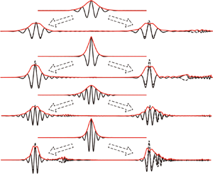
Short small-amplitude internal waves separated from breather-like waves in all cases at  $t/T_b\approx 1$ as illustrated in the comparisons of the Hilbert transform and the theoretical breather envelopes (figures 3 and 4). Since the group velocity of the short internal waves is slower than the linear long-wave speed, these waves move off to the right relative to the centres of the packets which in the plots are shifted so they are aligned at different times. The emission of these linear dispersive waves results in an energy loss from the leading nonlinear wave. In the case of $h/H = 0.25$ (figure 3), more short dispersive waves are released compared to cases with $h/H = 0.30$ (figure 4) because the ratio of the initial amplitude to the upper and lower layer depths, $4qH/h$, is larger for smaller $h/H$, which means that cases with $h/H = 0.25$ undergo stronger adjustment. In cases 7 and 8 ( $h/H = 0.30$), the density interface initially crosses the critical depth ( $h/H = 0.346$) and there is shedding of larger-amplitude waves and greater decay of the amplitude of the envelope obtained by the Hilbert transform (figure 4c,d). Additionally, among the cases with $h/H = 0.25$, cases 3 and 4 ( $q = 0.06/4$) were found to release more short internal waves compared to cases 1 and 2 ( $q = 0.03/4$). This suggests that the larger $q$ is, the more short small-amplitude internal waves are released, which is not surprising because of their higher nonlinearity. Interestingly, the wavelength of breathers, $\lambda _b$, does not change very much even after the emission of short internal waves.

Figure 3. Interface displacements for the upper and lower layers (solid and dashed lines), and envelopes obtained using the Hilbert transform for the upper layer (red lines) for cases 1 to 4 ( $h/H = 0.25$). Each panel shows initial interface displacement and two typical interface displacements, which correspond to the maximum and minimum amplitude cases shifted as indicated so that the centres align. (a) Case 1, (b) case 2, (c) case 3 and (d) case 4.

Figure 4. Same as figure 3 but for cases 5 to 8 ( $h/H = 0.30$). (a) Case 5, (b) case 6, (c) case 7 and (d) case 8.
In all cases the release of short internal waves results in a decrease in the breather amplitude  $a_H/H$ (figures 5 and 6). Here $a_H/H$ estimated from the maximum interface displacement (see figure 3a) is different from the Hilbert transform $a_H/H$ immediately after the initial condition, but they almost coincide when $t/T_b > 1$ for all cases. Amplitude $a_H/H$ is equal to the amplitude of breathers at the initial condition. In cases 1 and 3 ( $p = 0.025$), the dominant period of the $a_H$ fluctuations was $\sim$1, whereas in cases 2 and 4 ( $p = 0.05$) it was more than 2. Therefore, the predominant period of the $a_H/H$ fluctuations is longer than $T_b$ when $p = 0.05$ (figure 5b). Interestingly, in cases 2 and 4, $a_H/H$ also undergoes slow fluctuations with periods of $t/T_b = 40$ and 20, respectively ( $p=0.05$; figure 5b). Therefore, there may be the possibility that larger $p$ can generate a large lower-frequency fluctuation component when $h/H$ is relatively small. In cases 5 and 7 ( $p = 0.025$), the Hilbert transform $a_H/H$ was a little larger than the computed $a_H/H$ (figure 6a). In contrast to $h/H = 0.25$, no low-frequency fluctuation is apparent in these cases, which may suggest that the smaller $h/H$ is, the more unstable the breathers progress (figure 6b).


Figure 6. Time series of  $a_H/H$ in cases 5 to 8 and cases 11 and 12 ( $h/H = 0.30$) (black lines). (Definition of $a_H$ is shown in figure 3a.) Green lines indicate $a_H/H$ from the Hilbert transform. Red circles, triangles, pluses and crosses correspond to the marks in figure 8. Green stars correspond to figure 7.
Cases 5 and 6 have the smallest emission of short internal waves from the time series of  $a_H/H$ (figure 4a,b), which may indicate that the internal waves in cases 5 and 6 most closely resemble breathers. If the internal waves in these cases are breathers, the envelope obtained from the Hilbert transform should agree with the theoretical solutions. However, it was found that a short internal wave component is present at $t/T_b = 5$ in case 6 (figure 7a). Although the Hilbert transform approaches the theoretical solution of the envelope at $t/T_b = 30.0$, short internal waves are involved, which means that it may be difficult for the initial waves based on theoretical breathers to progress without any deformation and decay (figure 7b).

Figure 7. Interface displacements and envelopes for the upper layer (black and red solid lines), and envelopes obtained by the Hilbert transform from the theory (black dashed lines) for case 6 ( $h/H = 0.30, q = 0.0075$ and $p = 0.050$). The envelope of the breather solution was obtained using (2.12) in which $q$ was found from $a_H$. Green solid lines (values on right-hand axes) are the difference of the Hilbert transform and the theoretical envelope. (a) Period $t/T_b = 5.0$ (left-hand green star in figure 6b) and (b) $t/T_b = 30.0$ (right-hand green star in figure 6b).
If  ${\rm \Delta} \rho / \rho _0$ and $h/H$ are fixed, $\lambda _e/H$ has a monotonic relation with $a_H/h$ (figure 8). As shown with the red marks in figures 5 and 6, we extracted three sets of $a_H/H$ and $\lambda _e/H$ values at the beginning and when $a_H/H$ has reduced to half the initial amplitude. The theoretical solution shows that the larger the amplitude is, the shorter the length of the breather (figure 8). Furthermore, the relationship between the breather width and amplitude in the computational results was found to be similar to that for theoretical breathers (see (2.13)). However, as $a_H/H$ increases, $\lambda _e/H$ in the computational results was slightly larger than the theoretical solution. Koop & Butler (Reference Koop and Butler1981), Grue et al. (Reference Grue, Friis, Palm and Rusas1997) and Choi & Camassa (Reference Choi and Camassa1999) showed the same tendency in the relationship between the wave amplitude and length of an internal solitary wave in a two-layer fluid system.

5. Discussion
Initially  $a_H/H = 4q$; however, the computed $a_H/H$ decreases in time. Figure 9 shows theoretical values of $| V_{gr}/c_0 |$ for breathers as a function of $a_H/H$ for the four pairs of $h/H$ and $p$ values. Also plotted are $a_H/H$ values for the breathers in the numerical simulations versus their average group velocity. In terms of $t/T_b$ the average group velocities were calculated over intervals of length 2.5 for cases 1 and 3, 22.5 for cases 2 and 4, 1.2 for cases 5 and 7, and 10 for cases 6 and 8. The computed group velocities agree with the theoretical values when $| V_{gr}/c_0 |$ was $\sim$0.1 (figure 9a,d). But, when the computed $| V_{gr}/c_0 |$ was less than 0.1, its values are larger than the theoretical value (figure 9c). In contrast, when the computed $| V_{gr}/c_0 |$ was greater than 0.1, the computed values are less than the theoretical value (figure 9b). For cases 7 and 8, the values in green are at times when the density interface crosses the critical depth (figure 9c,d). To investigate the effect of the sign of $V_{gr}/c_0$, four additional simulations were done using small-amplitude initial conditions (cases 13 to 16). For these simulations we chose the smaller value of $q$ used in cases 1–8 because we found that the adjustment of the initial wave was smaller for this value of $q$. Positive $V_{gr}/c_0$ requires that $p < q \sqrt {3} \approx 0.00427$ so we considered $p=0.0001$ and $0.004$ for both $h/H = 0.25$ and $0.3$. In all four of these cases, the breather that emerged from the initial condition had $V_{gr}/c_0<0$. The computed $V_{gr}/c_0$ was $-6.3 \times 10^{-3}$ in cases 13 and 14 and $-5.2 \times 10^{-3}$ in cases 15 and 16, which shows no dependence of $V_{gr}/c_0$ on $p$.
$p$.

Figure 9. Comparisons of group velocity. Solid lines indicate the direction of group velocity that is opposite to the propagation direction of a long wave by (2.14). Dashed lines indicate that the direction of group velocity is the same as a long wave by (2.14). (a) Cases 1 and 3. (b) Cases 2 and 4. (c) Cases 5 and 7. (d) Cases 6 and 8.
To investigate the generation of short internal waves, we return to cases 7 and 8 in which the initial density interfaces cross the critical depth (figure 10). In these cases short small-amplitude internal waves separated from the breather with the rapid decrease in  $a_H/H$ (enclosed in red curves in figure 10) and we conjecture that this occurs because the density interfaces crossed the critical depth in cases 7 and 8. Additional short small-amplitude internal waves emerged gradually, continually reducing the amplitude of breathers (figure 10, blue-enclosed regions). These small-amplitude internal waves result in a gradual decrease in the amplitude of the initial theoretical breathers. For a two-layer fluid under the Boussinesq approximation the quadratic nonlinear term is zero when the interface is at the mid-depth and importantly internal solitary waves are limited in amplitude by the conjugate flow limit in which the interface is displaced to the mid-depth (Lamb & Wan Reference Lamb and Wan1998). Tsuji & Oikawa (Reference Tsuji and Oikawa2007) also showed that the amplification rate of soliton resonance is suppressed as the interface approaches the critical depth where the quadratic nonlinear term vanishes and dispersion prevails in the KdV equation. For the case of the breathers it is possible that there is an amplitude limitation and it occurs at the location where the cubic nonlinear coefficient vanishes and dispersion prevails in the mKdV equation ( $h/H=9/26$), which is similar to the critical depth in the KdV equation. To investigate the effect of the critical depth on the suppression of the amplitude, four additional simulations were done using large-amplitude initial conditions: case 9 with $(h/H, q, p) = (0.25, 0.0225, 0.025)$; case 10 with $(h/H, q, p) = (0.25, 0.0225, 0.050)$; case 11 with $(h/H, q, p) = (0.30, 0.0225, 0.025)$; and case 12 with $(h/H, q, p) = (0.30, 0.0225, 0.050)$ (table 1, figures 6 and 11). For cases 9 and 10 when $h/H = 0.25$, the initial density interfaces do not cross the critical depth, and we found that cases 9 and 10 are similar to cases 3 and 4 though initial $a_H/H$ in cases 9 and 10 is larger than in cases 3 and 4. On the other hand, when $h/H = 0.3$, the critical amplitude, defined as the distance between the undisturbed density interface and the critical depth, is 0.0462. The initial amplitude of cases 11 and 12 is 1.95 times larger than the critical amplitude while the amplitude of cases 7 and 8 is 1.3 times larger than the critical amplitude. In cases 11 and 12, $a_H/H$ decreases rapidly compared to cases 7 and 8 (figure 6). Short large-amplitude internal waves separated rapidly from the initial conditions and the amplitude of cases 11 and 12 decreased more rapidly, which is similar to that found by Tsuji & Oikawa (Reference Tsuji and Oikawa2007) and Nakayama et al. (Reference Nakayama, Kakinuma and Tsuji2019a) for solitary waves (figure 11). Additionally, Lamb et al. (Reference Lamb, Polukhina, Talipova, Pelinovsky, Xiao and Kurkin2007) shows the release of short large-amplitude internal waves under the condition when $h/H=0.3$, $p=0.0285$ and $q=-0.026$, which is similar to case 11, though $q$ is slightly larger than in our study. Therefore, the release of short large-amplitude internal waves and the rapid decrease in the amplitude may be because the initial density interfaces cross the critical depth in cases 7 and 8, but this cannot explain a similar emission of short large-amplitude internal waves in cases 3 and 4 for which the initial amplitude is below the critical amplitude. We also computed conjugate flow amplitudes for our two stratifications (Lamb & Wilkie Reference Lamb and Wilkie2004) and found that the limiting amplitudes for solitary waves are $a_{lim}/H = 0.15$ and 0.23 for $h/H = 0.3$ and 0.25, respectively, which exceed the distances of 0.096 and 0.046 to the critical depth. Hence displacement of the interface to the critical depth is not a limitation for internal solitary wave amplitudes. The model used in Lamb et al. (Reference Lamb, Polukhina, Talipova, Pelinovsky, Xiao and Kurkin2007) is based on the Navier–Stokes equations, and it is possible to consider more general stratifications, including higher-mode waves which can complicate the wave field. On the other hand, our model is a multilayer model, and we can ignore the effect of pycnocline thickness on waves, which eliminates mode-3 and higher waves. Therefore, it is easy to make direct comparisons with theoretical solutions. Since breathers are long waves (at least in the context of the Gardner equation), a finite thickness of the pycnocline is not expected to significantly affect wave profiles.

Figure 10. Space and time contour of the upper interface displacement for (a) case 7 and (b) case 8. Reference frame moved with the theoretical envelope speed,  $c_0 + V_{gr}$.

Figure 11. Interface displacements for the upper and lower layers  $(h/H = 0.30)$ at a time when the interface displacement was a maximum. (a) Case 11 with $(q, p) = (0.0225, 0.025)$. (b) Case 12 with $(q, p) = (0.0225, 0.050)$.
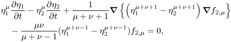
From the perspective of the energy scale, (2.22)–(2.28), it is expected that energy may rapidly reduce in cases 3, 4, 7 and 8 ( $q = 0.06/4$) when the amplitudes are relatively larger because many short internal waves are released. In cases 3 and 7 (figures 12c and 13c), $E_T$ initially decreased rapidly for a short period of time. In the other cases the initial decay rate ( $t/T_b<0.1$) was much smaller. This suggests that initial attenuation is relatively large when the initial amplitude is large and $p$ is small, which corresponds to larger $a_H$ and $\lambda _b$. On the other hand, in all cases $KE_1$, $KE_3$, $PE_1$ and $PE_1$ were found to have nearly the same energy scale. In fully nonlinear simulations, the movement of the interfaces means that fluid in the middle layer is moving so theoretically $KE_2$ should not be zero. In particular, in case 4 ( $h/H = 0.25$ with the maximum $p$ and $q$), the value of $KE_2$ was the largest among all cases and the attenuation rate of $E_T$ was also the largest. Therefore, it may be suggested that the second-mode kinetic energy is likely to be generated when $h/H$ and $\lambda _b$ are smaller.

Figure 12. Time series of potential energy and kinetic energy normalized by  $E_e$ in cases 1 to 4 ( $h/H = 0.25$). (a) Case 1, (b) case 2, (c) case 3 and (d) case 4.
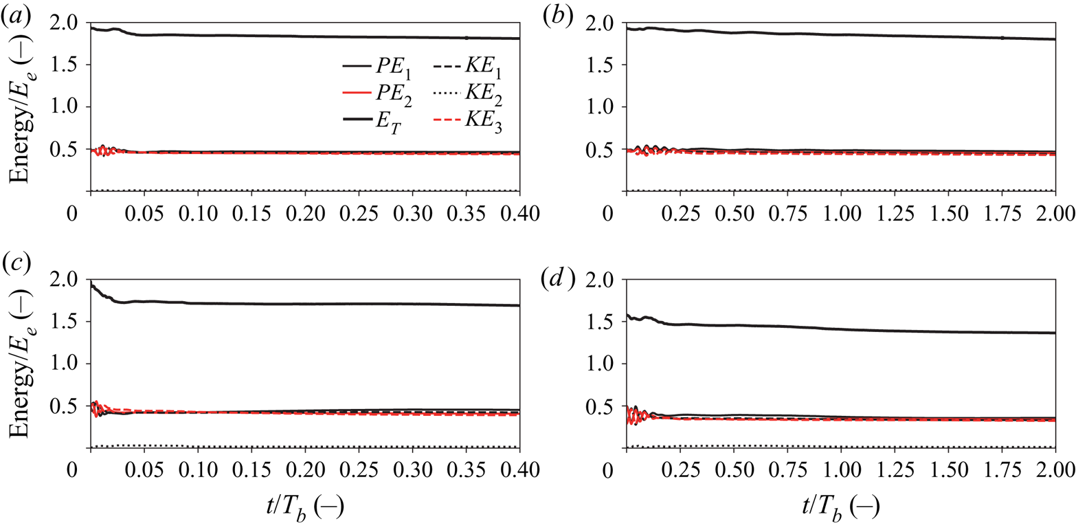
Figure 13. Time series of potential energy and kinetic energy normalized by  $E_e$ in cases 5 to 8 ( $h/H = 0.30$). (a) Case 5, (b) case 6, (c) case 7 and (d) case 8.
The breather amplitude is found to decrease due to the release of short internal waves since (2.7) is only a weakly nonlinear solution in a three-layer system. In addition to the critical depth, the release of short internal waves may be partially due to the mismatch of the displacements of the lower and upper interfaces, which results in the presence of second-mode kinetic energy (figures 12 and 13). The second-mode kinetic energy is less in the case of  $h/H=0.30$ than $h/H=0.25$. For small $h/H$ the interfaces are near the boundary and the upward displacement of the upper interface will be inhibited by the upper boundary while the lower interface does not have the suppression as an upper bound on its upward displacement. Similarly the downward displacement of the lower interface will be inhibited by the lower boundary. This introduces an asymmetry in the displacements of the two interfaces which should be expected for non-infinitesimal waves. Such asymmetries are present in mode-1 internal solitary waves and conjugate flows. This introduces an asymmetry that is not present in the leading-order vertical structure but it does arise at higher order (Grimshaw et al. Reference Grimshaw, Pelinovsky and Talipova1997). Figure 2 of Lamb et al. (Reference Lamb, Polukhina, Talipova, Pelinovsky, Xiao and Kurkin2007) shows the same mismatch of the displacements of the lower and upper interfaces.
6. Conclusion
The initial wave profile normalized by the total water depth,  $H$, was plotted as functions of $x/\lambda _b$ so that the initial wave profile depends only on $p$ and $q$, not on the cubic nonlinear coefficient and the dispersion coefficient. The relationship of the length and amplitude of the breathers from the computational results normalized by $H$ was found to be the same as for the theoretical solution (figure 8). For cases 1 to 4 ( $h/H = 0.25$), it was found that the larger $q$ is, the more short small-amplitude internal waves are released with a corresponding decrease in the amplitude and the broadening of the length of the breather. Interestingly, the wavelength of the carrier waves does not change appreciably, i.e. $p$ does not significantly change even after the emission of short internal waves. For $p=0.025$, the group velocity in the simulations was similar to the theoretical value; however, for the larger $p=0.05$ and smaller $h/H$, the group velocity in the simulations was considerably lower (see figure 9b). Therefore, when $h/H$ is relatively small, there may be the possibility that larger $p$ can generate lower-frequency fluctuations. For cases 5 to 8 ( $h/H = 0.30$), short internal waves are still generated though the Hilbert transform approaches the theoretical solution of the envelope. In cases 7, 8, 11 and 12 when the initial density interfaces cross the critical depth, the emission of short internal waves was enhanced. The cubic nonlinear coefficient vanishes on the critical depth ( $h/H=9/26$) and dispersion prevails in the mKdV equation. Therefore, the critical depth may be a significant factor controlling the amplitude of breathers in a three-layer fluid. Our simulations suggest that larger values of $h/H$ are better able to produce breathers in our nonlinear model.
Acknowledgements
This work was supported by the Japan Society for the Promotion of Science under grants 18H01545 and 18KK0119.
Declaration of interests
The authors report no conflict of interest.


 Open access