





Introduction
Soybean is a major crop in the United States, covering a national harvested area of 32.5 million ha in 2025 (USDA-NASS 2025). Planting date can substantially affect soybean growth and yield (Hu and Wiatrak Reference Hu and Wiatrak2012). A delay in soybean planting can result in a significantly smaller yield, resulting in a decrease of 13.6 kg per day when a crop is planted after the end of April (Hankinson et al. Reference Hankinson, Lindsey and Culman2015; Rattalino Edreira et al. Reference Rattalino Edreira, Mourtzinis, Conley, Roth, Ciampitti, Licht, Kandel, Kyveryga, Lindsey, Mueller, Naeve, Nafziger, Specht, Stanley, Staton and Grassini2017). This could mean a loss of approximately US$17,000 on a 40-ha field when soybean is planted on May 30th compared with May 1st, based on 2025 soybean prices. Additionally, fewer days are becoming suitable for fieldwork, with a loss of 1.77 days per decade since 1995 between April 7th and May 12th in Ohio (K-State Fieldwork Capacity Tool 2025). Due to fewer days that are suitable for performing fieldwork during the season and yield penalties from planting late, farmers tend to plant their soybean crops early. When a soybean crop is planted early, the seedlings may encounter cold temperatures and wet soils, which can lead to a significant reduction in plant population. An air temperature of 4 C when the crop is planted may inhibit germination, prolong germination time, and result in decreased plant height and dry weight (Wang et al. Reference Wang, Li, Zhou, Song and Dong2023). However, when fewer soybean plants need to compete for sunlight and soil nutrients the number of branches per plant increases, and the pods per branch, seeds per pod, and seed weight all increase (Stivers and Swearingin Reference Stivers and Swearingin1980). A soybean crop that is planted early has yielded more despite longer emergence times and fewer plants (Knott et al. Reference Knott, Herbek and James2019). A recent trial (2022) in Ohio showed that soybean planted ultra-early produces the highest yields, with up to 6,523 kg ha−1 when planted as early as March 30 (Kannberg et al. Reference Kannberg, Lindsey, Chiavegato and Lindsey2024). For comparison, the average yield for all of Ohio was 3,732 kg ha−1 in 2022 (USDA-NASS 2026). A few factors may contribute to yield increases from early planting, including a longer total growth period, resulting in increased biomass, and a longer seed-filling period (Egli Reference Egli2011). Also, an early planting date has been associated with earlier development of reproductive stages, which can help avoid pressures from late-summer drought, insects, and plant diseases (Salmeron et al. Reference Salmeron, Gbur, Bourland, Buehring, Earnest, Fritschi, Golden, Hathcoat, Lofton, Miller, Neely, Shannon, Udeigwe, Verbree, Vories, Wiebold and Purcell2014).
Although there are benefits to planting early, potential reductions in plant population and slowed growth pose a significant threat to achieving rapid canopy closure, a key cultural method of weed suppression (Jha and Norsworthy Reference Jha and Norsworthy2009). Cultural weed control via canopy closure is effective because it limits sunlight from reaching weeds, compromising their germination, establishment, and photosynthetic capabilities (Norsworthy and Oliveira Reference Norsworthy and Oliveira2007; Sanyal et al. Reference Sanyal, Bhowmik, Anderson and Shrestha2008). Planting date greatly influences when and which herbicides to use because weed species differ in their emergence timing, with each species exhibiting a relatively distinct emergence window (Hilgenfeld et al. Reference Hilgenfeld, Martin, Mortensen and Mason2004). Environmental conditions influence these emergence patterns and can vary substantially by geographic location (Chudzik et al. Reference Chudzik, Nunes, Arneson, DeWerff, de Sousa Ferreira, Proctor, Stoltenberg, Conley and Werle2025), potentially affecting the strategy and efficacy of herbicide applications. In addition to planting date, a few management practices affect canopy closure and soybean yield, including row spacing, tillage system, and herbicide programs (Arsenijevic et al. Reference Arsenijevic, DeWerff, Conley, Ruark and Werle2022). Among these, herbicide use can be highlighted as the primary method of weed control (Harker and O’Donovan Reference Harker and O’Donovan2013), making it necessary to develop a herbicide program specifically designed to address the fundamental issues of early planting and delayed canopy closure. Therefore, the objective of this study was to evaluate herbicide combinations and timing for their effect on weed development and soybean yield when a soybean crop is planted ultra-early (before April 15th in Ohio) and during normal planting times (early to mid-May in Ohio).
Materials and Methods
Experimental Design and Site Description
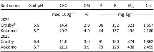
Field experiments were conducted during two growing seasons, 2024 and 2025, at the Western Agricultural Research Station, in South Charleston, Ohio (39.859187°N 83.672371°W). Two fields with different soil types were used each year, a Strawn-Crosby complex (Fine, mixed, active, mesic Aeric Epiaqualfs) and a Kokomo silty clay loam (Fine, mixed, superactive, mesic Typic Argiaquolls), for a total of 4 site-years (Crosby-24 and Crosby-25, and Kokomo-24 and Kokomo-25). The fields were not tilled. Soybean had been planted the previous year, except for Crosby-25 where corn (Zea mays L.) had been planted the previous year. All 4 site-years were sampled before planting to a depth of 15 cm for analysis of soil chemical properties (Table 1).
Soil properties of experimental fields. a
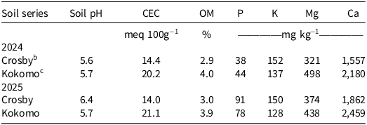
Table 1. Long description
The table presents soil properties of experimental fields for two growing seasons, 2024 and 2025, at the Western Agricultural Research Station in South Charleston, Ohio. It includes data for two soil types: Crosby and Kokomo. The table has five columns: Soil series, Soil pH, CEC in milliequivalents per 100 grams, OM in percentage, P in milligrams per kilogram, K in milligrams per kilogram, Mg in milligrams per kilogram, and Ca in milligrams per kilogram. The table has five rows, including a header row. For 2024, Crosby soil has a pH of 5.6, CEC of 14.4, OM of 2.9 percentage, P of 38 milligrams per kilogram, K of 152 milligrams per kilogram, Mg of 321 milligrams per kilogram, and Ca of 1,557 milligrams per kilogram. Kokomo soil for 2024 has a pH of 5.7, CEC of 20.2, OM of 4.0 percentage, P of 44 milligrams per kilogram, K of 137 milligrams per kilogram, Mg of 498 milligrams per kilogram, and Ca of 2,180 milligrams per kilogram. For 2025, Crosby soil has a pH of 6.4, CEC of 14.0, OM of 3.0 percentage, P of 91 milligrams per kilogram, K of 150 milligrams per kilogram, Mg of 374 milligrams per kilogram, and Ca of 1,862 milligrams per kilogram. Kokomo soil for 2025 has a pH of 5.7, CEC of 21.1, OM of 3.9 percentage, P of 78 milligrams per kilogram, K of 128 milligrams per kilogram, Mg of 438 milligrams per kilogram, and Ca of 2,459 milligrams per kilogram.
a Abbreviations: Ca, calcium; CEC, cation exchange capacity; K, potassium; Mg, magnesium, OM, organic matter; P, phosphorus.
b Fine, mixed, active, mesic Aeric Epiaqualfs
c Fine, mixed, superactive, mesic Typic Argiaquolls
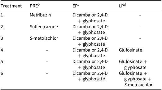
The experimental unit consisted of seven rows of soybean spaced 38 cm apart, with an additional 19 cm on each side of the plot, totaling 3 m of width and 9 m of length (27 m2). In Ohio, 38 cm is the most common row width for soybean (Mourtzinis et al. Reference Mourtzinis, Rattalino Edreira, Grassini, Roth, Casteel, Ciampitti, Kandel, Kyveryga, Licht, Lindsey, Mueller, Nafziger, Naeve, Stanley, Staton and Conley2018). The design was a randomized complete block design with a split-plot arrangement and four replications. The main factor was planting date: ultra early (before April 15) and normal (early to mid-May). The subplot factor was herbicide treatment with six levels (Table 2).
Herbicides applied at preemergence, early postemergence, and late postemergence. a
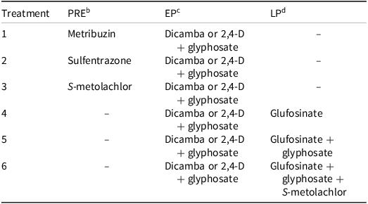
Table 2. Long description
The table presents herbicide treatments applied at preemergence, early postemergence, and late postemergence stages of soybean growth. It consists of six rows and three columns. The columns are labeled Treatment, PRE, EP, and LP. Each row lists a different herbicide treatment and the specific herbicides applied at each stage. For example, Treatment 1 includes Metribuzin at PRE, Dicamba or 2,4-D plus glyphosate at EP, and no herbicide at LP. Treatment 6 includes no herbicide at PRE, Dicamba or 2,4-D plus glyphosate at EP, and Glufosinate plus glyphosate plus S-metolachlor at LP. The table provides a detailed comparison of various herbicide combinations used at different growth stages.
a Abbreviations: EP, early postemergence; LP, late postemergence; PRE, preemergence.
b PRE herbicides included metribuzin (Sencor, 420 g ai ha−1; Bayer); sulfentrazone (Spartan, 351 g ai ha−1; FMC); and S-metolachlor (Dual Magnum, 1,782 g ai ha−1; Syngenta).
c In 2024, herbicides applied at EP included dicamba (XtendiMax, 560 g ai ha−1; Bayer) and glyphosate (RoundUp PowerMax 3, 1,255 g ae ha−1; Bayer). In 2025, herbicides applied at EP included 2,4-D (Enlist One, 1,065 ai ha−1; Corteva) and glyphosate.
d Herbicides applied at LP included glufosinate (Liberty, 656 g ai ha−1; BASF); glyphosate (RoundUp PowerMax 3, 1,255 g ae ha−1; Bayer), and S-metolachlor (Dual Magnum, 1,782 g ai ha−1, Syngenta)
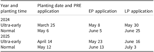
The cultivar used in 2024 was AG33XF3 XtendFlex (Bayer Crop Science, St. Louis, MO) with maturity group 3.3. In 2025, the variety used was P35Z76E Enlist E3 (Corteva Agriscience, Indianapolis, IN), with maturity group 3.5. XtendFlex was replaced by Enlist E3 technology in 2025 due to changes in herbicide regulations over dicamba use. Seeds were planted 2.5 cm deep and at a seeding rate of 383,000 seeds ha−1. In 2024, on the day of planting, a burndown application of glyphosate (RoundUp PowerMax 3, 1,255 g ae ha−1, Bayer) and dicamba (XtendiMax, 560 g ai ha−1, Bayer) was applied. In 2025, glyphosate and 2,4-D (Enlist One, 1,065 g ai ha−1, Corteva) were applied as the burndown. Preemergence herbicide treatments were applied the day of planting. All herbicides were applied using the rate specified on the product label. Early postemergence herbicides were applied after 400 growing degrees days (GDD: 10 C base temperature) following planting. An early postemergence application based on GDD was used because of the possibility of extremely different planting dates that could affect weed growth, leading to unreliable triggering based on weed height. GDD has been used to estimate the critical time of weed removal (CTWR) in soybean (Soltani et al. Reference Soltani, Shropshire and Sikkema2022) and the time to postemergence herbicide applications to sugarbeet (Dale and Renner Reference Dale and Renner2005). Late postemergence treatments were applied 21 d after early postemergence. Herbicides were applied using a CO2-pressurized backpack sprayer with a volume of 140 L ha−1, a speed of 4.8 km h−1, a boom length of 3 m, a pressure of 331 kPa, using TTI110015 (TeeJet Technologies, Glendale Heights, IL) nozzle. Planting and application dates were the same in both fields within each year (Table 3).
Soybean planting dates and dates of herbicides applied at preemergence, early postemergence, and late postemergence. a
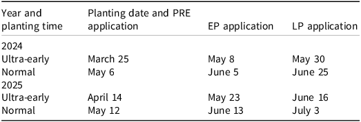
Table 3. Long description
The table presents soybean planting dates and the corresponding herbicide application timings for the years 2024 and 2025. It includes three columns: Year and planting time, Planting date and PRE application, EP application, and LP application. The table has four rows, with the first row indicating the year and the subsequent rows detailing planting times as Ultra-early and Normal. For 2024, the planting dates are March 25 for Ultra-early and May 6 for Normal. The corresponding EP application dates are May 8 and June 5, and the LP application dates are May 30 and June 25. For 2025, the planting dates are April 14 for Ultra-early and May 12 for Normal. The corresponding EP application dates are May 23 and June 13, and the LP application dates are June 16 and July 3.
a Abbreviations: EP, early postemergence; LP, late postemergence; PRE, preemergence.
Data Collection
Soybean plant population density was recorded when each planting date achieved the V2 (two open trifoliolates) and R8 (soybean maturity) growth stages by counting every plant in two rows of 5.3 m and converting to number of plants per hectare (plants ha−1). Canopy coverage of the weeds and the soybean crop was assessed with the Canopeo mobile app (Oklahoma State University), which quantifies the percentage of green leaf area in an image using fractional green canopy coverage (Patrignani and Ochsner Reference Patrignani and Ochsner2015). Two subsamples were taken at the same location in each plot weekly, two pictures with a black cardboard (30.5 cm wide by 76.2 cm long) placed between soybean rows to cover weeds and capture only soybean canopy coverage, and two pictures without cardboard capturing the total green leaf area in the image (Dias Mendonça et al. Reference Dias Mendonça, Lindsey, Essman and Lindsey2026). Weed canopy coverage was estimated by subtracting soybean green leaf area from the total green leaf area.
Weed density was recorded just before the early postemergence and late postemergence applications, 14 d and 28 d after the early postemergence and late postemergence applications, respectively, and before harvest using a 0.25-m2 quadrat placed randomly in the plot. Weeds inside the quadrat were separated by species and counted, then extrapolated to number of plants per hectare. Biomass was also recorded at early postemergence and late postemergence using the 0.25-m2 quadrat, clipping the weeds at the soil level inside the quadrat, and separating them into grass and broadleaves. The weed samples were dried at 60 C for 3 d and then weighed. Weed canopy height was measured on 10 subsample plants at both postemergence timings and averaged across species.
Visual evaluation of herbicide damage to soybean plants was conducted at 3, 7, 14, 21, and 28 d after emergence using a percentage scale: 0% indicated no visible signs of herbicide injury, and 100% indicated complete plant mortality. Visual evaluation of weed control was assessed at early postemergence and late postemergence applications and 28 d after early postemergence and late postemergence, using a percentage scale for each species: 0% indicated no control, and 100% indicated total control of weeds.
Yield was recorded with an 8-XP (Kincaid Equipment Manufacturing, Haven, KS) plot combine, and moisture was corrected to 13%. However, for the first planting date in 2024, due to extreme weed density at the time of harvest, soybean plants were hand-harvested from two rows of 5.3 m in length, processed with an SPT-1A thresher (Agriculex, Guelph, ON, Canada), and moisture was measured with a Mini GAC 2500 moisture analyzer (DICKEY-john, Auburn, IL) to correct grain weight to 13% moisture.
Statistical Analysis
Data were analyzed for each site-year individually with the GLIMMIX procedure (SAS/STAT software), and means were separated using the GLIMMIX procedure. P-values for differences (PDIFF) of the least significant means test for pairwise comparisons at α = 0.05. Site-years were analyzed separately due to differences in planting dates between the two years, weather differences (a freeze in 2024), and weed populations. The linear mixed model included planting date, herbicide treatment, and their interaction as fixed effects, and replicates and planting dates within replicates (to accommodate the split-plot design) as random effects. Residual normality was checked with Q-Q plots, residual vs. prediction plots, and Shapiro-Wilk test. Transformations were applied when necessary to meet the assumptions of normality of residuals: square root for weed biomass, log(weed density + 1), and arcsine of the square root for visual evaluation of weed control. The back-transformed means are presented herein.
Soybean canopy coverage was regressed over time using the R package minpack.lm (v. 4.5.1; R Core Team 2025) following a four-parameter logistic model: $y = a + {{b - a} \over {1 + exp\left[ { - c*\left( {x - d} \right)} \right]}}$
where $y$
is soybean canopy coverage,
$y$
is soybean canopy coverage, $x$
is Julian date, a is the lower asymptote, b is the upper asymptote, c is the steepness, and d is the inflection point. Parameters a and b were fixed at zero and 100, respectively, to ensure biological sense. Essentially making the model a two-parameter logistic (c and d as parameters), and the inflection point (d) representing the Julian day on which canopy coverage reached 50%.
$x$
is Julian date, a is the lower asymptote, b is the upper asymptote, c is the steepness, and d is the inflection point. Parameters a and b were fixed at zero and 100, respectively, to ensure biological sense. Essentially making the model a two-parameter logistic (c and d as parameters), and the inflection point (d) representing the Julian day on which canopy coverage reached 50%.
Results and Discussion
Weather Conditions
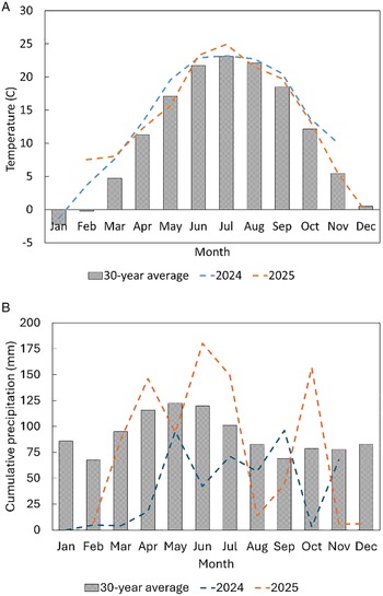
Monthly average temperature and cumulative precipitation for both years are shown in Figure 1. Average temperatures were slightly higher than the 30-yr average in both years. Temperature and photoperiod are well-known factors that influence the flowering date of soybean (Garner and Allard Reference Garner and Allard1930; Sinclair et al. Reference Sinclair, Kitani, Hinson, Bruniard and Horie1991). When planted early, soybean plants are exposed to longer nights before the summer solstice, which can lead to early flowering (Bastidas et al. Reference Bastidas, Setiyono, Dobermann, Cassman, Elmore, Graef and Specht2008). In both years, soybeans planted ultra-early also exhibited early flowering, with flower bud development appearing as early as May 28th in 2024. This early flowering can be attributed to above-average temperatures and an extremely early planting date, which could also limit spraying capabilities in a commercial setting, because soybean plants are particularly sensitive to synthetic auxin herbicides after flowering, which can cause a significant reduction in pods per plant (Solomon and Bradley Reference Solomon and Bradley2014). Also, some postemergence herbicides, such as glufosinate, glyphosate, and 2,4-D, have label restrictions on applying after a certain reproductive stage, usually R1 or R2 (BASF 2023; Bayer 2021; Corteva 2024).
Average monthly temperature (A) and cumulative precipitation (B) for both seasons compared with the 30-yr average.
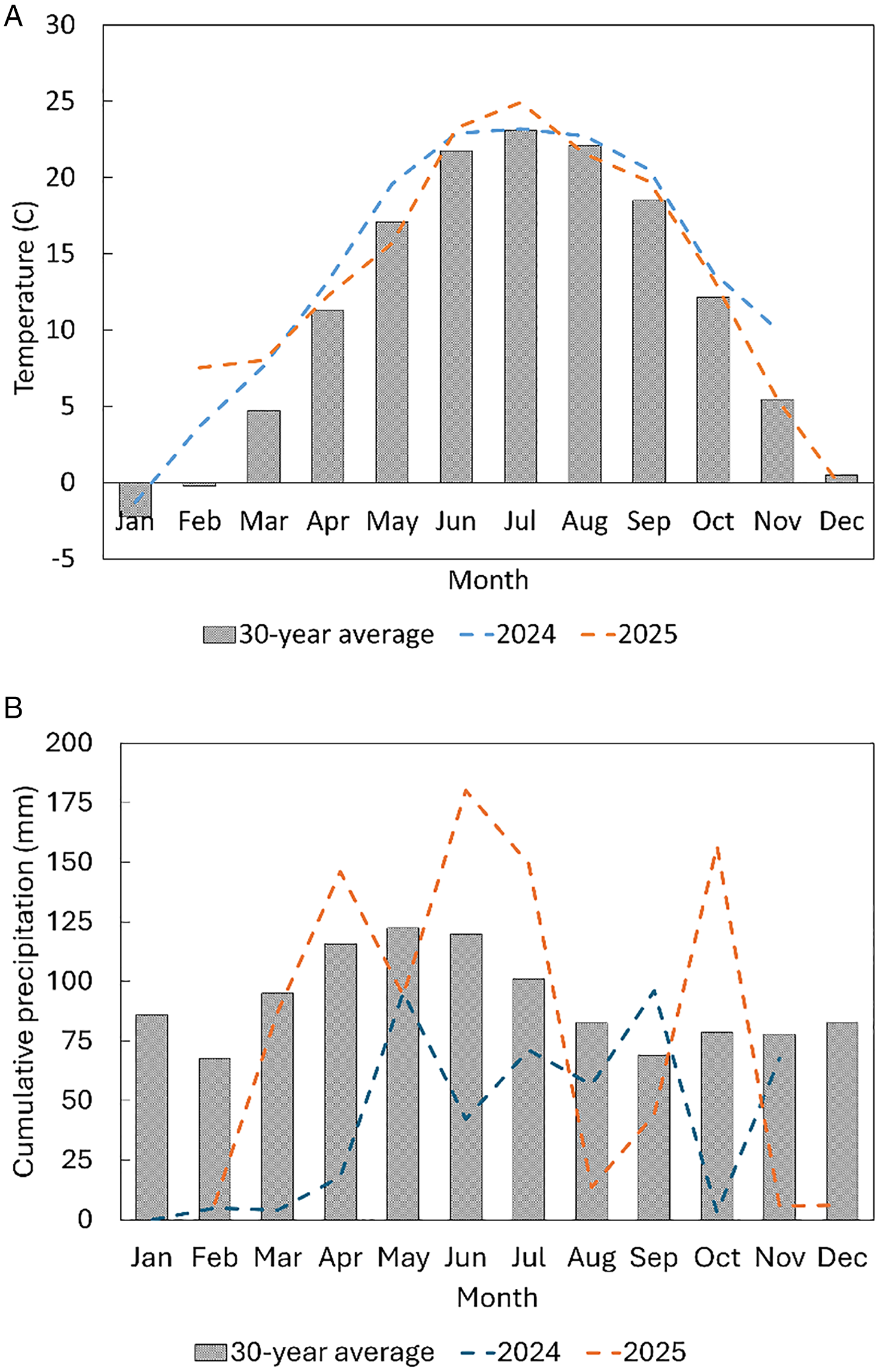
Figure 1. Long description
The image contains two graphs. The first graph (A) is a combination of bar and line graphs showing average monthly temperature in degrees Celsius. The x-axis represents the months from January to December, and the y-axis represents the temperature ranging from -5 to 30 degrees Celsius. The bar graph shows the 30-year average temperature for each month. The line graphs represent the temperatures for the years 2024 and 2025, with 2024 depicted by a blue dashed line and 2025 by an orange dashed line. The second graph (B) is a combination of bar and line graphs showing cumulative precipitation in millimeters. The x-axis represents the months from January to December, and the y-axis represents the cumulative precipitation ranging from 0 to 200 millimeters. The bar graph shows the 30-year average cumulative precipitation for each month. The line graphs represent the cumulative precipitation for the years 2024 and 2025, with 2024 depicted by a blue dashed line and 2025 by an orange dashed line. The graphs illustrate how the temperatures and precipitation in 2024 and 2025 compare to the 30-year average.
Cumulative precipitation differed between the two growing seasons. The 2024 growing season was very dry, with nearly every month recording precipitation below the 30-yr average, whereas precipitation in 2025 was generally above the 30-yr average (Figure 1). A noteworthy freeze occurred on April 22, 2024, which substantially affected the plant population of the soybeans than had been planted ultra-early and consequently reduced its weed suppression capability that year.
Soybean Evaluations
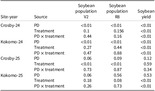
Soybean plant population at the V2 and R8 stages showed a main effect of planting date in both fields during the 2024 growing season (Table 4), with the ultra-early planting date experiencing an average reduction of approximately 70% (Table 5). Stressful conditions, such as cold and wet soil can lead to emergence inhibition and population loss, something that occurs with several crops, including soybean (Collier et al. Reference Collier, Spaner, Graf and Beres2020; Haidar et al. Reference Haidar, Lackey, Charette, Yoosefzadeh-Najafabadi, Gahagan, Hotte, Belzile, Rajcan, Golshani, Morrison, Cober and Samanfar2023; Neththasinghe et al. Reference Anuththara Neththasinghe, Wilson, Lindsey and Lindsey2025; Zhou et al. Reference Zhou, Muhammad, Lan and Xia2022). Although population differences among planting dates can be partially attributed to emergence inhibition, the substantial 70% decrease observed in the ultra-early planting date was most likely caused by the freeze on April 22nd, which killed many plants.
Analysis of variance for fixed effects of planting date, herbicide treatment, and their interaction on soybean evaluations. a
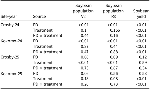
Table 4. Long description
The table presents an analysis of variance for fixed effects of planting date, herbicide treatment, and their interaction on soybean evaluations. It includes data for different site-years, such as Crosby-24, Kokomo-24, Crosby-25, and Kokomo-25. The table has four columns: Site-year, Source, Soybean population V2, Soybean population R8, and Soybean yield. Each row provides p-values for the effects of planting date, treatment, and their interaction on soybean population at the V2 and R8 stages, as well as soybean yield. Notable trends include significant effects of planting date on soybean population and yield, with ultra-early planting dates showing a substantial reduction in population due to stressful conditions and freeze events.
a Abbreviations: PD, planting date; R8, soybean reproductive stage 8 (maturity); V2, soybean growth stage 2.
Soybean plant population at V2 and R8 stages affected by planting date of four site-years. a

Table 5. Long description
The table presents data on soybean plant population at the V2 and R8 stages, affected by planting dates across four site-years. It consists of five rows and five columns. The columns are labeled Population, Planting date, Crosby-24 plants per hectare, Kokomo-24 plants per hectare, Crosby-25 plants per hectare, and Kokomo-25 plants per hectare. The rows are labeled Soybean at V2 and Soybean at R8, with sub-rows for Ultra-early and Normal planting dates. Notable data points include a significant reduction in plant population for the ultra-early planting date, with approximately a 70% decrease attributed to a freeze on April 22nd. For example, at the V2 stage, the ultra-early planting date shows 89,883 plants per hectare for Crosby-24 and 79,278 plants per hectare for Kokomo-24, compared to 290,945 and 293,946 plants per hectare, respectively, for the normal planting date. Similar trends are observed at the R8 stage and for the Crosby-25 and Kokomo-25 varieties.
a Abbreviations: R8, soybean reproductive stage 8 (maturity); V2, soybean growth stage 2.
Injury to soybean plants from preemergence-applied herbicides was minimal (data not shown), in contrast to previous research showing that soybean planted early in cold, wet conditions exhibited greater injury and yield reductions from preemergence herbicides (Poston et al. Reference Poston, Nandula, Koger and Matt Griffin2008). The lack of soybean damage from herbicides is likely due to nonconducive environmental conditions, with dry and above-average temperatures in 2024 and later planting dates and above-average temperatures in 2025 (Figure 1). Reports of soybean injury and yield response to preemergence herbicides are mixed; some studies documented the occurrence of injury with no yield penalty (Arsenijevic et al. Reference Arsenijevic, de Avellar, Butts, Arneson and Werle2021; Kandel et al. Reference Kandel, Mueller, Legleiter, Johnson, Young and Wise2018), whereas others reported both significant injury and yield loss (Poston et al. Reference Poston, Nandula, Koger and Matt Griffin2008), including recommendations for spraying preplant instead of preemergence to avoid crop injury (Priess et al. Reference Priess, Norsworthy, Roberts and Gbur2020). It is also important to note that soils with high pH (>7) and low amounts of organic matter are more conducive to injury from the herbicides sulfentrazone and metribuzin (Arsenijevic et al. Reference Arsenijevic, de Avellar, Butts, Arneson and Werle2021). These conditions did not exist in this study, because soil pH ranged from 5.6 to 6.4 and organic matter ranged from 2.9% to 4.0% (Table 1).
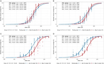
Soybean canopy closure was severely delayed by planting ultra-early in 2024, with the date of 50% canopy coverage (parameter d, the inflection point in Equation 1) being very similar across planting dates despite a 42-d gap between them (Figure 2). Similarly, previous research with peanut (Arachis hypogaea L.) has shown reduced canopy coverage when the crop is planted early (Kharel et al. Reference Kharel, Devkota, Macdonald, Tillman and Mulvaney2022). In contrast, canopy development in 2025 followed a more typical pattern, with slight differences in parameter d, likely due to the later ultra-early planting date and absence of frost damage. These 2025 canopy coverage results align with findings that showed a faster canopy closure occurring in soybean planted in late April compared with late May (Arsenijevic et al. Reference Arsenijevic, DeWerff, Conley, Ruark and Werle2022). This is likely due to a later first planting date than in 2024, when soybean plants were subjected to much harsher early season stresses and resulted in a different canopy coverage trend. In Figure 2B, treatments 4 through 6 exhibited a delayed canopy closure early in the season (prior to 50% closure) compared with canopy closure that occurred after Treatments 1 through 3 under ultra-early planting conditions. This delay could be explained by the prevalence of grass weeds in that specific site-year.
Soybean canopy coverage regression curves across planting dates (PD) and treatment groups 1–3 and 4–6, at Crosby-24 (A), Kokomo-24 (B), Crosby-25 (C), and Kokomo-25 (D). Treatment groups were pooled based on programs that included similar herbicide application timings (treatment groups 1–3 included preemergence followed by early postemergence herbicide applications and groups 1–4 included postemergence followed by late postemergence applications. The model equation is $y = a + \;{{b - a} \over {1 + \exp \left[ { - c*\left( {x - d} \right)} \right]}}$
. Parameters are explained in Equation 1. The model coefficient a was set to zero in all cases, and model coefficient b was set to 100 to denote biological limits for canopy development.
$y = a + \;{{b - a} \over {1 + \exp \left[ { - c*\left( {x - d} \right)} \right]}}$
. Parameters are explained in Equation 1. The model coefficient a was set to zero in all cases, and model coefficient b was set to 100 to denote biological limits for canopy development.
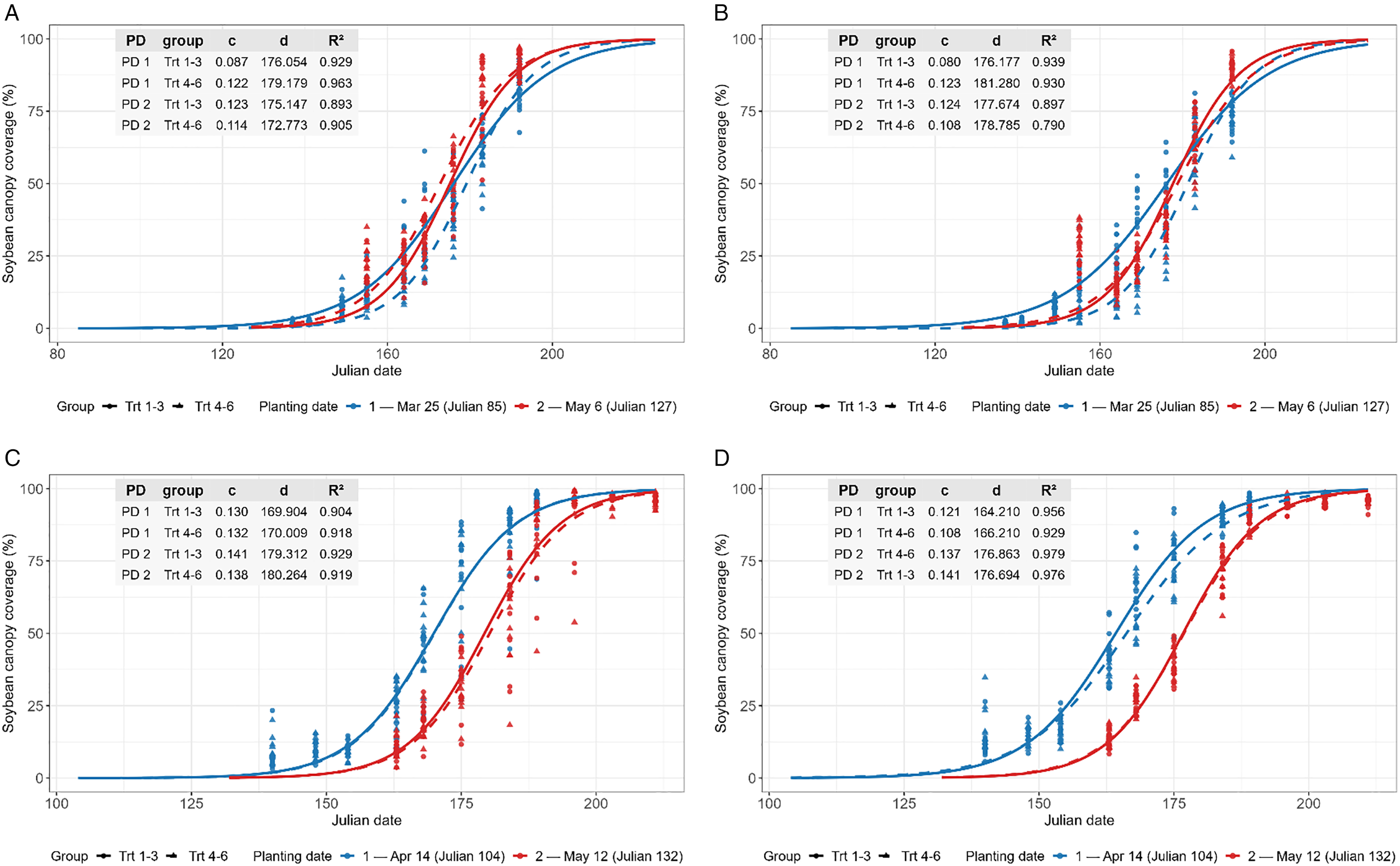
Figure 2. Long description
The image contains four line graphs labeled A, B, C, and D, each representing soybean canopy coverage across different planting dates and treatment groups at locations Crosby-24, Kokomo-24, Crosby-25, and Kokomo-25. The x-axis represents the Julian date, and the y-axis represents soybean canopy coverage in percentage. Each graph includes two planting dates, March 25 and May 6 for graphs A and B, and April 14 and May 12 for graphs C and D. The treatment groups are divided into Trt 1-3 and Trt 4-6, with different herbicide application timings. The graphs show regression curves with parameters c and d, and R-squared values indicating the fit of the model. The curves illustrate how soybean canopy coverage changes over time for different planting dates and treatment groups. All values are approximated.
Row width likely played a role in canopy closure and weed suppression dynamics. Narrow row spacing (38 cm) has been shown to facilitate faster canopy closure than wider row spacing (76 cm) (Arsenijevic et al. Reference Arsenijevic, DeWerff, Conley, Ruark and Werle2022). However, even planting in 38-cm rows was not sufficient to offset the environmental stress caused by planting ultra-early, which resulted in delayed canopy closure and limited weed suppression compared with the normal planting date.
Weed Evaluations
The most common weed species at all site-years were giant foxtail (Setaria faberi Herrm.), giant ragweed (Ambrosia trifida L.), velvetleaf (Abutilon theophrasti Medik.), common lambsquarters (Chenopodium album L.), and redroot pigweed (Amaranthus sp. L.). However, giant foxtail and giant ragweed were substantially more abundant than the other species. Therefore, our reports focus primarily on those two weeds. Although giant foxtail was the most common grass species, all grass species were grouped together for reporting purposes. In 2024, grasses were more prevalent at the Crosby location, whereas the Kokomo location was more heavily infested with giant ragweed. In contrast, weed pressure was minimal at Crosby in 2025 but remained moderate for giant ragweed at Kokomo. The giant ragweed population in this experiment was resistant to herbicides in Groups 2 and 9 (as categorized by the Weed Science Society of America and the Herbicide Resistance Action Committee.
Average weed height when herbicides were applied at early postemergence was 112 mm at Crosby-24, 118 mm at Kokomo-24, 80 mm at Crosby-25, and 110 mm Kokomo-25. At late postemergence, the average weed height was 83 mm, 66 mm, 107 mm, and 122 mm for the Crosby-24, Kokomo-24, Crosby-25, and Kokomo-25, site-years respectively. Weed heights at both application timings were within the height range for applying postemergence herbicides according to the product labels (BASF 2023; Bayer 2021; Corteva 2024; Syngenta 2024).
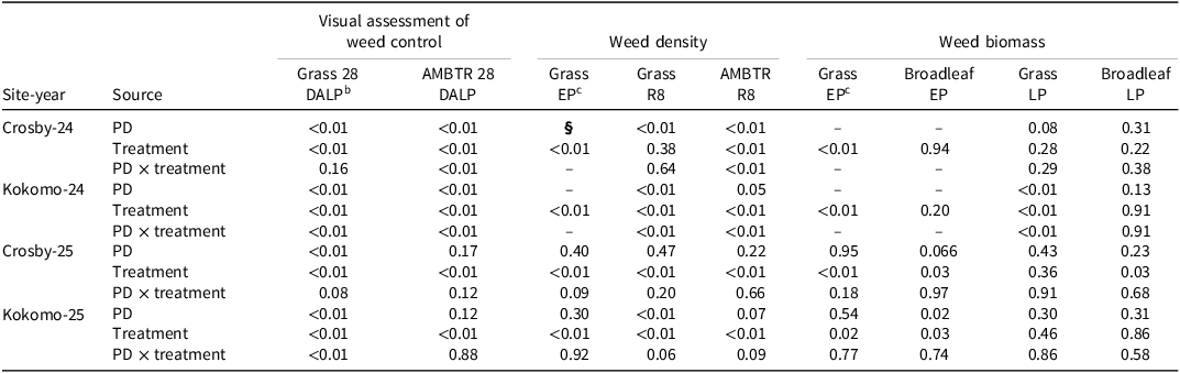
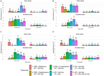
There were no consistent significant differences in weed canopy coverage (data not shown). Planting date and herbicide treatment main effect, as well as their interactions on weed biomass, weed density, and visual assessment of weed control can be found in Table 6. There was minimal planting date effect on weed biomass, while herbicide treatment had a significant effect, especially at the early postemergence application timing. This is further detailed in Figure 3, which shows that weed biomass at the early postemergence timing was clearly different depending on preemergence herbicides. Grass biomass was significantly reduced when S-metolachlor was applied as a preemergence herbicide, especially in Kokomo-24, when grass infestation was highest, reducing biomass from 63 g m−2 in Treatment 1 to 14 g m−2 in Treatment 3. In contrast, Treatment 1, when metribuzin was applied preemergence, had the lowest broadleaf weeds biomass in 2025, with approximately an 85% reduction compared with Treatment 3. These findings align with previous research that reported better grass control from metolachlor (a mixture of S- and R- metolachlor isomers), compared to metribuzin, and superior broadleaf control from metribuzin compared to that of metolachlor (Oliveira et al. Reference Oliveira, Feist, Eskelsen, Scott and Knezevic2017). Treatment 2, which included sulfentrazone applied preemergence, provided effective control of both grass and broadleaf weeds, indicating it to be a reliable option regardless of the weeds present. As expected, Treatments 4, 5, and 6 demonstrated similar biomass at the early postemergence timing given that no herbicide had been applied prior to data collection. Likewise, similar weed biomass at the late postemergence timing is due to the broad-spectrum herbicides applied to all plots at early postemergence.
Analysis of variance for fixed effects of planting date, herbicide treatment, and their interaction on weed evaluations, including visual assessment of weed control of grass and giant ragweed at 28 d after late postemergence, weed density of grass and giant ragweed at soybean maturity and weed biomass of grass and broadleaf weeds at early postemergence and late postemergence. a
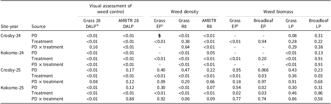
Table 6. Long description
The table presents the analysis of variance for fixed effects of planting date, herbicide treatment, and their interaction on weed evaluations. It includes visual assessment of weed control for grass and giant ragweed at 28 days after late postemergence, weed density of grass and giant ragweed at soybean maturity, and weed biomass of grass and broadleaf weeds at early and late postemergence. The table has 8 rows and 11 columns. The columns are labeled as follows: Site-year, Source, Visual assessment of weed control (Grass 28 DALP, AMBTR 28 DALP), Weed density (Grass EP, Grass R8, AMBTR R8), and Weed biomass (Grass EP, Broadleaf EP, Grass LP, Broadleaf LP). The rows are labeled with different site-years (Crosby-24, Kokomo-24, Crosby-25, Kokomo-25) and factors (PD, Treatment, PD x treatment). Notable trends include significant effects of herbicide treatment on weed biomass, particularly at early postemergence application timing. Planting date effects on weed biomass were minimal. Specific data points show significant reductions in grass biomass with S-metolachlor application and broadleaf weed biomass with metribuzin application.
a Abbreviations: AMBTR, Bayer code for giant ragweed (Ambrosia trifida L.); DALP, days after late postemergence; EP, early postemergence; LP, late postemergence; PD, planting date; R8, soybean reproductive stage 8 (maturity).
b Primarily composed of giant foxtail (Setaria faberi Herrm.) with other grass species present; therefore, results are reported as total grasses.
c EP evaluations were not collected for the ultra-early planting date in 2024.
Weed biomass across herbicide treatments at early postemergence and late postemergence application timings at Crosby-24 (A), Kokomo-24 (B), Crosby-25 (C), and Kokomo-25 (D). Herbicide treatments included metribuzin, sulfentrazone, and S-metolachlor applied preemergence (PRE); synthetic auxin (SA, dicamba or 2,4-D) and glyphosate (Gly) applied early postemergence (EP); and glufosinate (Glu), glyphosate (Gly), and S-metolachlor (S-met) applied late postemergence (LP). Different letters within a graph panel denote that means were significantly different from one another.
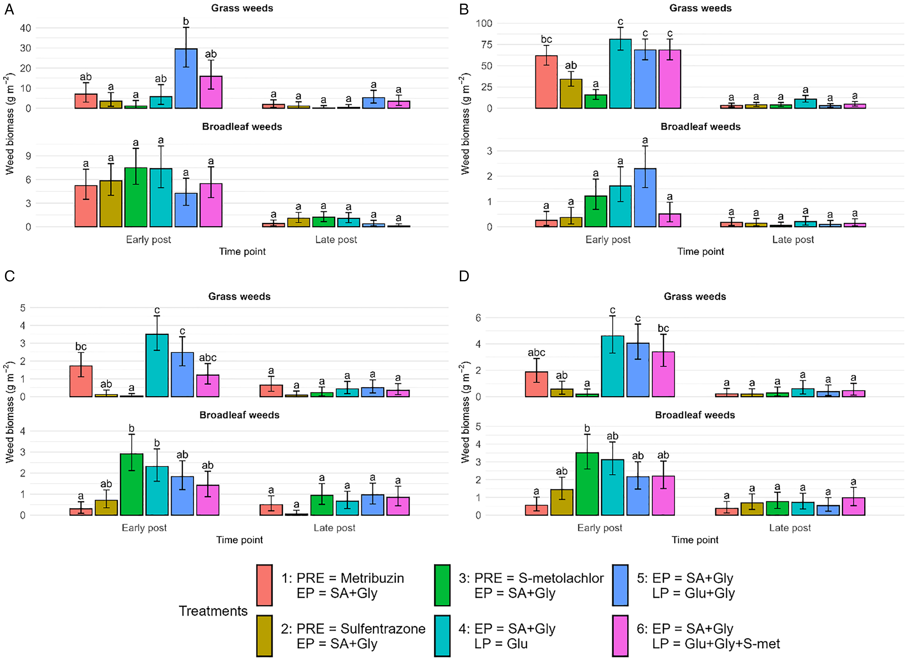
Figure 3. Long description
The image contains four sets of bar graphs labeled A, B, C, and D, each showing weed biomass for grass weeds and broadleaf weeds at early postemergence and late postemergence application timings. The graphs compare the effects of different herbicide treatments, including metribuzin, sulfentrazone, and S-metolachlor applied preemergence; synthetic auxin and glyphosate applied early postemergence; and glufosinate, glyphosate, and S-metolachlor applied late postemergence. Each set of graphs represents data from different locations: Crosby-24, Kokomo-24, Crosby-25, and Kokomo-25. The x-axis represents the time points (early post and late post), and the y-axis represents weed biomass in grams per square meter. Different letters within each graph panel denote significant differences in means. The color-coded bars represent various herbicide treatments, with specific colors indicating different combinations of treatments. All values are approximated.
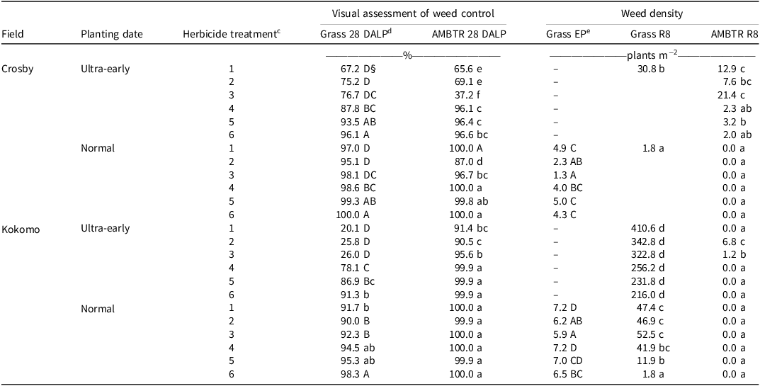
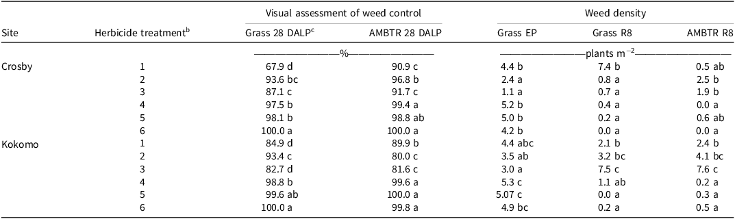
Weed density and visual assessment of control of velvetleaf, lambsquarters, and redroot pigweed were excluded from analysis due to a high frequency of zero plants per square meter and 100% control ratings, resulting in non-normally distributed data. There was no significant effect of planting date or herbicide treatment on weed density at the time of both postemergence applications (data not shown), except for a treatment effect on grass density at early postemergence (Table 6). Grass density averages were consistently lower across site-years for Treatments 2 and 3 compared with the other herbicide treatments (Tables 7 and 8).
Visual assessment of weed control and weed density affected by planting date and herbicide treatment for two fields in 2024.a,b
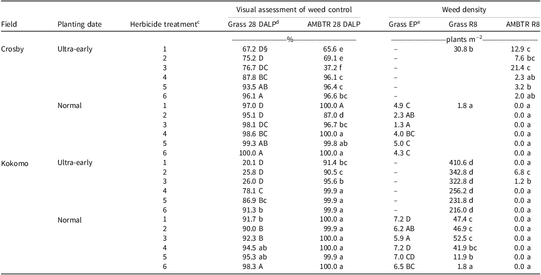
Table 7. Long description
The table presents data on the visual assessment of weed control and weed density affected by planting date and herbicide treatment for two fields in 2024. It includes columns for field names, planting dates, herbicide treatments, visual assessment percentages for grass and AMBTR at 28 days after last planting, and weed density measurements for grass at early postemergence and at the reproductive stage 8, as well as for AMBTR at stage 8. The table has 24 rows and 10 columns. Notable trends include consistently lower grass density averages for Treatments 2 and 3 compared to other herbicide treatments. The data highlights the impact of different herbicide treatments and planting dates on weed control and density.
a Abbreviations: AMBTR, Bayer code for giant ragweed (Ambrosia trifida L.); DALP, days after late postemergence; EP, early postemergence; LP, late postemergence; PD, planting date; PRE, preemergence; R8, soybean reproductive stage 8 (maturity).
b Capital letters reflect differences only between herbicide treatments, where no interaction with planting date was detected
c Herbicide treatments: 1, metribuzin applied PRE, dicamba or 2,4-D + glyphosate applied EP; 2, sulfentrazone applied PRE, dicamba or 2,4-D + glyphosate applied EP; 3, S-metolachlor applied PRE, dicamba or 2,4-D + glyphosate applied EP; 4, dicamba or 2,4-D + glyphosate applied EP, glufosinate applied LP; 5, dicamba or 2,4-D + glyphosate applied EP, glufosinate + glyphosate applied LP; 6, dicamba or 2,4-D + glyphosate applied EP, glufosinate + glyphosate + S-metolachlor applied LP.
d Primarily composed of giant foxtail (Setaria faberi Herrm.) with other grass species present; therefore, results are reported as total grasses.
e Grass density at EP was not collected for the ultra-early planting date in 2024.
Visual assessment of weed control and weed density affected by herbicide treatment for two fields in 2025, averaged across planting dates. a
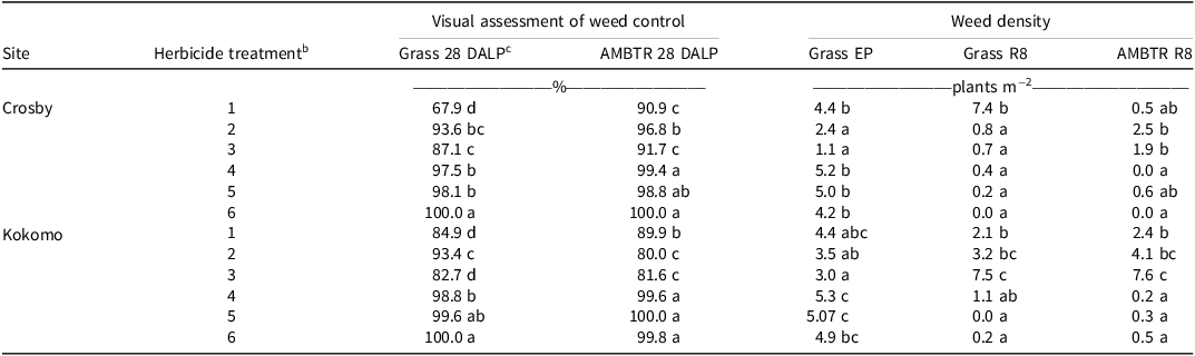
Table 8. Long description
The table presents data on the visual assessment of weed control and weed density affected by herbicide treatments for two fields in 2025, averaged across planting dates. It includes two sites, Crosby and Kokomo, each with six herbicide treatments. The columns detail the visual assessment of weed control for grass and AMBTR at 28 days after late preemergence, and weed density for grass at early postemergence and grass and AMBTR at late postemergence. The data shows varying levels of weed control and density across different treatments and sites. For instance, Treatment 1 at Crosby shows 67.9 percent grass control and 90.9 percent AMBTR control, with a grass density of 4.4 plants per square meter at early postemergence. Treatment 6 at Kokomo shows 100 percent grass control and 99.8 percent AMBTR control, with a grass density of 4.9 plants per square meter at early postemergence. Notable trends include consistently lower grass density for Treatments 2 and 3 across site-years compared to other herbicide treatments.
a Abbreviations: AMBTR, Bayer code for giant ragweed (Ambrosia trifida L.); DALP, days after late postemergence; EP, early postemergence; LP, late postemergence; PRE, preemergence; R8, soybean reproductive stage 8 (maturity).
b Herbicide treatments: 1, metribuzin applied PRE, dicamba or 2,4-D + glyphosate applied EP; 2, sulfentrazone applied PRE, dicamba or 2,4-D + glyphosate applied EP; 3, S-metolachlor applied PRE, dicamba or 2,4-D + glyphosate applied EP; 4, dicamba or 2,4-D + glyphosate applied EP, glufosinate applied LP; 5, dicamba or 2,4-D + glyphosate applied EP, glufosinate + glyphosate applied LP; 6, dicamba or 2,4-D + glyphosate applied EP, glufosinate + glyphosate + S-metolachlor applied LP.
c Primarily composed of giant foxtail (Setaria faberi Herrm.) with other grass species present; therefore, results are reported as total grasses.
In Kokomo-24, visual grass control at 28 d after late post (DALP) was poor for Treatments 1, 2, and 3, with 20%, 26%, and 26% of control respectively (Table 7), whereas Treatments 5 and 6 were superior in the ultra-early planting date, at 87% and 91% respectively. Similarly, Miller et al. (Reference Miller, Landau, Williams and Hager2025) reported greater weed control by including postemergence applications instead of just preemergence applications at 28 DALP to early planted soybean. Despite these visual weed control differences, grass density at soybean maturity at Kokomo-24 was statistically similar across all herbicide treatments in the ultra-early planting date, ranging from 216 to 411 plants m−2, while Treatment 6 resulted in the lowest grass density at the normal planting date (1.8 plants m−2). These results highlight the challenge of achieving effective grass control when soybean is planted extremely early, with densities going as high as 411 plants m−2 under Treatment 1.
In Crosby-24, Treatment 3 resulted in the lowest visual control of giant ragweed at 28 DALP in the ultra-early planting date (37.2%), whereas Treatment 6 had the highest control (96.6%) (Table 7). Treatment 6 also provided the lowest giant ragweed density (2 plants m−2), whereas the highest density (21 plants m−2) occurred with Treatment 3.
Previous research has shown that giant ragweed can achieve up to 95% emergence as late as early July (Wuerffel et al. Reference Wuerffel, Young, Matthews, Davis, Johnson and Young2015) and that early planted soybean can have higher giant ragweed densities compared with late-planted soybean when the soil has been tilled (Chudzik et al. Reference Chudzik, Nunes, Arneson, DeWerff, de Sousa Ferreira, Proctor, Stoltenberg, Conley and Werle2025). This literature aligns with the results we observed in the present study and supports the superiority of herbicide treatments that contain two postemergence applications when giant ragweed pressure is high and when crops are planted early, because populations can have a wide window of emergence and escape early season herbicide applications. Additionally, including a residual herbicide in later postemergence applications can further enhance weed control in programs targeting giant ragweed when planting crops ultra-early.
In 2025, there was a main effect of herbicide treatment for visual assessment of weed control and weed density (Table 6), when the ultra-early planting date occurred later than in 2024 and planting date differences were less prominent. Nonetheless, treatment differences in 2025 followed a similar pattern as the one observed in 2024: Treatments 1, 2, and 3 (preemergence + early postemergence) were generally inferior to Treatments 4, 5, and 6 (early postemergence followed by (fb) late postemergence) (Table 8).
Residual dissipation is an important factor that may explain the reduced performance of preemergence fb early postemergence application of herbicides. Because the sites had not been tilled, the residual dissipation effect may have been enhanced, as previous researchers have reported that S-metolachlor dissipates more quickly in no-till fields than tilled fields where soybeans have been planted early (Chudzik et al. Reference Chudzik, Arneson, DeWerff, Mobli, Mueller and Werle2026).
When soybean plants are planted ultra-early, emergence and canopy development are both delayed. This reduces the agronomic advantage of applying preemergence herbicides. Since soybean development is delayed when planted ultra-early, soil-applied herbicides can lose their residual effect before the crop and weeds emerge. Therefore, preemergence fb early postemergence treatments were less effective at providing season-long weed suppression in crops planted ultra-early.
Soybean Yield
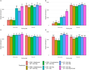
There was a planting date × herbicide treatment interaction for soybean yield in all site-years, except for Crosby-625 (Table 4). In 2024, regardless of herbicide treatment, yields at all four locations were statistically similar and highest overall when soybean crops were planted at the normal time (Figure 4). The lowest yields from crops that were planted ultra-early were recorded when treatments included a preemergence herbicide fb an early postemergence herbicide, regardless of the preemergence herbicide used. Yields from crops treated with an early postemergence herbicide fb a late postemergence herbicide were approximately three times greater, on average, than the preemergence fb early postemergence routine. Treatment 6, which included S-metolachlor as a residual herbicide at late postemergence, consistently produced the greatest yield from any crop planted ultra-early, and yields were statistically similar to those of crops that had been planted at the normal date in the Crosby field, despite the 70% difference in soybean plant population between planting dates. With low plant populations, soybean plants compensate by increasing the number of side branches, pods, and seeds they produce while often maintaining yield (Cox and Cherney Reference Cox and Cherney2011; Cox et al. Reference Cox, Cherney and Shields2010).
Soybean grain yield across planting date and herbicide treatments at Crosby-24 (A), Kokomo-24 (B), Crosby-25 (C), and Kokomo-25 (D). Herbicide treatments included metribuzin, sulfentrazone, and S-metolachlor applied preemergence (PRE); synthetic auxin (SA, dicamba or 2,4-D) and glyphosate (Gly) applied early postemergence (EP); and glufosinate (Glu), glyphosate (Gly), and S-metolachlor (S-met) applied late postemergence (LP). Different letters within a graph panel denote means that were significantly different from one another.
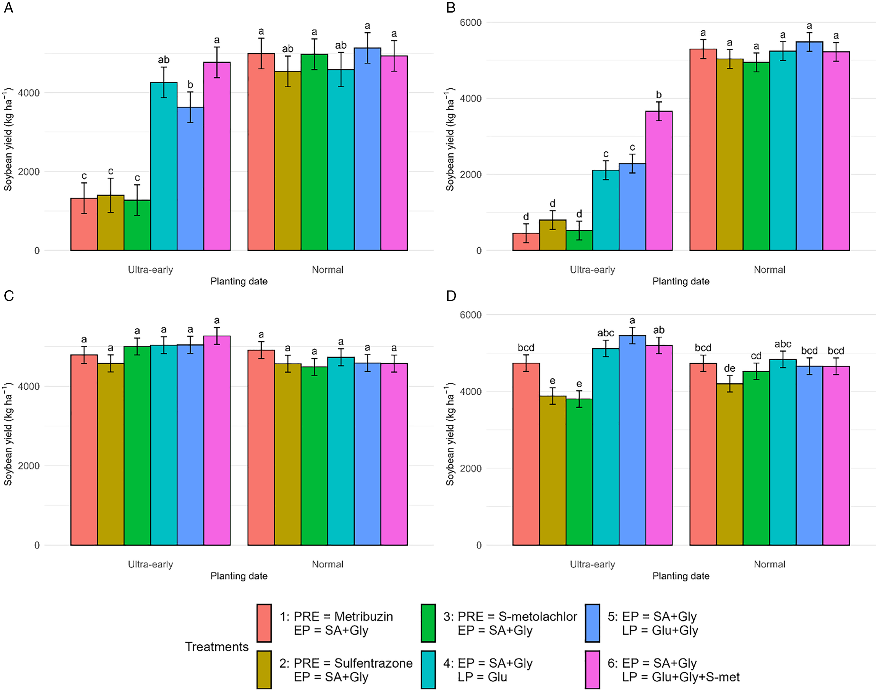
Figure 4. Long description
The bar graph compares soybean grain yield across different planting dates and herbicide treatments at four locations: Crosby-24, Kokomo-24, Crosby-25, and Kokomo-25. The x-axis represents the planting date categories: Ultra-early and Normal. The y-axis represents the soybean yield in kilograms per hectare. There are four panels labeled A, B, C, and D, each representing a different location and year. Each panel contains six vertical bars representing different herbicide treatments: metribuzin, sulfentrazone, and S-metolachlor applied preemergence; synthetic auxin and glyphosate applied early postemergence; and glufosinate, glyphosate, and S-metolachlor applied late postemergence. The bars are color-coded: red for metribuzin, orange for sulfentrazone, green for S-metolachlor, blue for synthetic auxin and glyphosate, teal for glufosinate, and pink for glufosinate, glyphosate, and S-metolachlor. Different letters within a graph panel denote means that were significantly different from one another. The graph shows that soybean yield varies significantly with planting date and herbicide treatment. All values are approximated.
In 2025, yield differences were fewer than in 2024 (Figure 4). There were no statistical differences at the Crosby site. However, at the Kokomo site, with the exception of Treatment 1, yields were smaller when soybean was planted ultra-early after being treated with a preemergence fb an early postemergence application than when they received two postemergence applications. Interestingly, among crops planted ultra-early that received Treatment 5, yields were statistically superior to those of crops planted at normal dates that received most herbicide treatments, demonstrating the potential for yield benefit of planting early when weed control is effective. Similar results were reported in Michigan, where soybean planted early (mid-April) produced yields that were similar to those of a typical planting date (mid-May) when weed control was adequate, but yield penalties occurred when control was inadequate (Goddard et al. Reference Goddard, Singh and Sprague2025).
Although planting date strongly influenced soybean canopy closure in these experiments, soybean yield response was closely linked to the effects of weed control provided by various herbicide treatments. Ultra-early planting extended the period to canopy closure and substantially affected the crop’s capability to compete with weeds. Herbicide treatments that entailed preemergence fb early postemergence applications failed to provide season-long weed control, especially under environmental stress and severe soybean plant loss in 2024, leading to significant yield decreases. Two postemergence applications provided more consistent weed control and preserved higher yields.
Practical Implications
Ultra-early soybean planting presents a demanding yet increasingly relevant challenge for farmers. Unfavorable weather often forces them to plant earlier than current recommendations. With that, our findings can elucidate good weed management practices for those conditions.
In general, an early postemergence fb a late postemergence application of herbicides consistently outperformed treatments of preemergence fb early postemergence applications in both weed control and soybean yield. In particular, Treatment 6, which includes S-metolachlor, applied at late postemergence, provided better season-long weed control when the crop was severely decreased because of a frost that occurred in 2024. This treatment also consistently resulted in higher yields, demonstrating soybean compensation capability when weed control is maintained through the season.
GDDs were used in this research as a way to standardize the early postemergence application timing across planting dates. However, the common unit of measurement in commercial and research settings is typically weed size. GDD-based or calendar-based methods should not be interpreted as direct recommendations for timing postemergence applications, since they could lead to weed sizes outside the optimal range for herbicide control. Effective scouting for determining weed height and density remains a priority when making postemergence application decisions.
Although these results favor two postemergence herbicide applications when crops are planted ultra-early, use of preemergence herbicides remains a critical tool for managing herbicide resistance and overall weed management under more typical environmental conditions. However, when crops are planted ultra-early, postemergence herbicides must be applied twice and it may be preferable to include a residual component to provide appropriate season-long weed control and to protect yield potential.
Acknowledgments
We thank Tony Dobbels, John McCormick, Allen Geyer, Joe Davlin, and staff members who work with authors A.J. Lindsey and A. Essman for their assistance with field work.
Funding
This research was funded by the Ohio Soybean Council. L.D. Mendonça received graduate student support from The Ohio Program (TOP) Fellowship.
Competing Interests
The authors declare they have no competing interests.



 Open access

